Embed Size (px)
Citation preview

ICAR - National Institute of Agricultural Economics and Policy Research
New Delhi
MANUAL ONMETHODOLOGICAL APPROACH FOR DEVELOPING
REGIONAL CROP PLAN
Under the ICAR Social Science Network Project Regional Crop Planning for Improving Resource Use Efficiency and Sustainability
Dr. Rajni JainDr. S.S. RajuDr. Kingsly ImmanuelrajDr. S. K. SrivastavaMrs. Amrit Pal KaurDr. Jaspal Singh

MANUAL ONMethodological approach for developing
regional crop plan
icar - national institute of agricultural economics and policy researchnew delhi
Dr. Rajni JainDr. S.S. Raju
Dr. Kingsly ImmanuelrajDr. S. K. SrivastavaMrs. Amrit Pal Kaur
Dr. Jaspal Singh
Under the icar Social Science network project Regional Crop Planning for Improving Resource Use Efficiency and Sustainability

ii Methodological Approach for Developing Regional Crop Plan
Manual onMethodological Approach for Developing Regional Crop Plan
Under the ICAR Social Science Network Project Regional Crop Planning for Improving Resource Use Efficiency and Sustainability
Authors
Dr. Rajni Jain
Dr. S.S. Raju
Dr. Kingsly Immanuelraj
Dr. S.K. Srivastava
Mrs. Amrit Pal Kaur
Dr. Jaspal Singh
© NIAP 2015
Published by
Dr. P. S. Birthal Acting Director, NIAP
Printed at
National Printers, B-56, Naraina Industrial Area, Phase-II, New Delhi - 110028 Tel. No. : 011-42138030, 09811220790

iiiMethodological Approach for Developing Regional Crop Plan
cONteNtS
Preface v
Acronyms and Abbreviations vii
List of Tables ix
List of Figures xi
List of Annexures xi
1 Introduction 1
1.1 Background 1
2 Data 3
2.1 Unit-level Cost of Cultivation Data: Extraction and Retrieving Procedure 3
3 Methodological Framework and Analytical Tools 10
3.1 Changes in cropping pattern 10
3.2 Changes in Land use pattern 11
3.3 Resource Use Efficiency 11
3.3.1 Data Envelopment Analysis (DEA) approach 12
3.4 Cost-Return Analysis 14
3.4.1 Net returns at market prices (NRMP) 14
3.4.2 Net returns at economic prices (NREP) 15
3.4.3 Net returns based on natural resource valuation(NRNRV) 19
3.5 Optimization of crop model 19
3.5.1 Mathematical specifications of the model 20
3.5.2 Objective Function: Maximization of net income (Equation 1) 20
3.5.3 Minimum and maximum constraints (Equation 3-4) 21
3.5.4 Ground water constraints 21
4 Optimum Crop Model for Punjab – A Case Study 23
References 35
Annexures 37

vMethodological Approach for Developing Regional Crop Plan
PRefAce
In various regions of India, cropping pattern is inefficient in terms of resource use and unsustainable from natural resource use point of view. This leads to serious misallocation
of resources, efficiency loss, indiscriminate use of land and water resources, and it adversely affecting long term production prospects. Indian agriculture confronts with many challenges and problems. Some of them can be formulated as optimization problems. Crop selection at regional level is one such challenge which can be addressed using optimum crop planning. As such regional crop planning is very crucial that helps to formulate region specific crop planning which would optimize the level of each activity of different crops, level of input use and output produced under different resource endowments and price scenarios.
This manual on “Methodological Approach for Developing Regional Crop Plan” has been drawn from the ICAR Social Science Network project “Regional Crop Planning for Improving Resource Use Efficiency and Sustainability”. The project has relied on plot level data collected by Directorate of Economics and Statistics, Ministry of Agriculture, Government of India under the Comprehensive Scheme for Studying the Cost of Cultivation of Principal Crops in India. The manual is aimed to provide the methodological approach for developing regional crop plans. The modelling framework has been illustrated with a case study of Punjab state.
The authors thankfully acknowledge the financial support received from ICAR and the technical advice and guidance extended by Prof. Ramesh Chand, Member, NITI Aayog and former Director, ICAR-NIAP.We are also thankful to all the associates and seven project collaborators from various agricultural universities of different agro-eco regions of India.
We would also like to place on record, our gratitude to the ICAR-NIAP for extending the necessary administrative and infrastructural support to develop this manual.
Authors


viiMethodological Approach for Developing Regional Crop Plan
AE Allocative efficiency
CCS Cost of Cultivation Survey
CE Cost Efficiency
CGWB Central Ground Water Board
CWC Central Water Commission
DEA Data Envelopment Analysis
DES Directorate of Economics and Statistics
DMU Decision Making Unit
EP Economic Prices
FAO Food and Agriculture Organization
GAMS General Algebraic Modeling System
GCA Gross Cropped Area
GHG Green House Gas
GoI Government of India
GoPb Government of Punjab
GR Gross Returns
HP Horse Power
K Potassium
LP Linear Programming
MP Market Prices
N Nitrogen
NR Net Returns
NRMP Net Returns at Market Prices
NREP Net Returns at Economic Prices
NRNRV Net Returns based on Natural Resource Valuation
NRV Natural Resource Valuation
P Phosphorous
RCP Regional Crop Planning
RGWAA Replenishable Ground Water Available for Agriculture
AcRONYMS AND ABBReVIAtIONS

viii Methodological Approach for Developing Regional Crop Plan
RGW-NREP Replenishable Ground Water- Net Returns at Economic Prices
RGW-NRMP Replenishable Ground Water- Net Returns at Market Prices
RGW-NRNRV Replenishable Ground Water –Net Returns at Natural Resource Valuation
RT’s Record Types
SAS Statistical Analysis System
SI Simpson’s Index
SRI System of Rice Intensification
TE Technical Efficiency
VC Variable Costs

ixMethodological Approach for Developing Regional Crop Plan
LISt Of tABLeS
Table 1 List of RT’s with the broad theme area 4
Table 2 Analytical tools used in the study 10
Table 3 Computation of NR MP for paddy in Punjab during TE 2010-11, (Rs/ha) 14
Table 4 Computation of Fertilizer subsidy for paddy in Punjab during TE 2010-11 16
Table 5 Estimation of Ground water extraction cost and ground water irrigation subsidy for paddy crop in Punjab during TE 2010-11
17
Table 6 Estimation of canal water irrigation subsidy for paddy crop in Punjab during TE 2010-11
18
Table 7 Computation of net returns at economic prices (NR EP) for paddy in Punjab during TE 2010-11, (Rs/ha)
18
Table 8 Computation of net returns based on NRV (NRNRV) for paddy in Punjab during TE 2010-11, (Rs/ha)
19
Table 9 Scenarios used for development of optimum crop models 23
Table 10 Optimum crop model for unrestricted GW use: Business as usual scenario 28
Table 11 Optimum crop model for GW use restricted to 20 BCM: Ground water sustainability scenario
29
Table 12 Gains due to optimum crop model over existing scenario 29


xiMethodological Approach for Developing Regional Crop Plan
LISt Of fIgUReS
Figure 1 MS-DOS for merging RT files (BIN format) 6
Figure 2 MS-DOS for merging RT files (BIN format) if they are given separately 7
Figure 3 DATAMAN Window Snapshot 7
Figure 4 DATAMAN Import and Export Utility Window 8
Figure 5 DATAMAN Window to specify data fields 8
Figure 6 Output file of DATAMAN in PRN format 9
Figure 7 SAS Software Window 9
Figure 8 Alternative ways to measure net returns of crops 14
Figure 9 Components of Cost A1 15
Figure 10 Excel sheet named ‘data’ for showing crop calendar for selected crops 24
Figure 11 Excel sheet named ‘limit’ for data inputs to GAMS program 24
Figure 12 GAMS code for developing RCP with code description 25
Figure 13 GAMS solve summary 30
LISt Of ANNexUReS
1 Economic valuation of nitrogen fixation and GHG emission by various crops 37
(a) Estimates of nitrogen fixed by legumes (Kg/ha) 37
(b) Economic contribution of legumes through nitrogen fixation (Rs/ha) 37
(c) Methane emission factors for paddy cultivation 38
(d) Green House Gas (GHG) emission from selected crops in India 38
2 GAMS basics for solving constrained optimization problems 39


1Methodological Approach for Developing Regional Crop Plan
1Introduction
MethODOLOgIcAL APPROAch fOR DeVeLOPINg RegIONAL cROP PLAN
Indian agriculture faces twin challenges of low growth and low per capita income on one hand, and ensuring food security of the nation on the other hand. Un-sustainability of
Indian agriculture and inefficient resource-use pattern recognized during the past four decades is well documented. The existing land use pattern of many states is not based on the principle of comparative advantage. The existing cropping pattern of various regions is inefficient in terms of resource use and unsustainable in terms of natural resource use. As such crop production will become more difficult with resource scarcity (e.g. land, water, energy, and nutrients), climate change and environmental degradation (e.g. deteriorating soil quality, increased greenhouse gas emissions etc.). The growth of agriculture in India largely depends on the enhancement in management of different resources. In this context, the question of allocation and distribution of resources in terms of sustainability, efficiency and optimization of crop plans across regions and production environments in the nation becomes vital. In the shifting paradigm of Indian agriculture, proper crop planning and policy plays a crucial role. However there is an absence of right set of policies and needed infrastructure to promote crop pattern consistent with regional resource endowment. As such Regional Crop Planning (RCP) is the need of the hour. RCP is a multi-dimensional concept, associated with determining the best set of crops to be cultivated over season with given constraints in the region. It involves area allocation for each of these crops, the sequencing of crops, and the irrigation plans. Best suitable crops and other enterprises should be selected so as to achieve some set of goals particular to the region. Typically, these goals involve the maximization of net income, the minimization of cost, the maximization of total area cultivated, and/or the minimization of irrigation water.
It becomes imperative to devise a standardized methodology for optimal crop plans. Therefore, this manual has been prepared to facilitate the development of regional crop plans using the common modeling framework. The methodological framework accompanies illustrations for the Punjab state, as case study, under the ICAR Social Science Network Project “Regional Crop Planning for Improving Resource Use Efficiency and Sustainability”.
1.1 BAcKgROUND
The project has been taken up in a network mode to cover almost all the agro-eco systems of the nation during the XII five-year plan. The study involves seven states from different agro-eco system, namely: (a) Irrigated -Punjab and Bihar; (b) Rain-fed – Maharashtra and Karnataka; (c) Coastal-Tamil Nadu; (d) Semi-Arid-Rajasthan and (e) North-East– Assam. The study has largely used the unit-level Cost of Cultivation Survey (CCS) data of Directorate of Economics and Statistics, Ministry of Agriculture, Government of India.

2 Methodological Approach for Developing Regional Crop Plan
With this background, the overall objective of the study is to develop regional crop plans for better resource use efficiency and improving natural resource sustainability across production environments. The major objectives of the study are:
1. To study the existing land use, cropping pattern, and resource use efficiency across regions
2. To estimate the cost and returns of selected crops under different regions of the country based on market prices, economic prices and natural resource valuation techniques.
3. To develop optimum crop plan at regional levels for better resource use efficiency, sustainability and maximizing farm net income across production environments.
sts

3Methodological Approach for Developing Regional Crop Plan
2Data
The study is primarily based on plot-level data collected under “Comprehensive Scheme for Cost of Cultivation of Principal Crops” of Directorate of Economics and Statistics,
Ministry of Agriculture. It is a rich source of data on the cost of cultivation of major crops, which also covers various aspects of farming across different regions of the country. It is uniform and representative data collected by conducting field surveys by identified nodal agencies in 17 states using uniform schedule and survey methodology. In the CCS, each sample household is surveyed consecutively for three years and the latest available data pertains to the period 2008-09 to 2010-11 (block year ending 2010-11). For Punjab, the plot-wise data was collected from the 300 representative households of 30 tehsils during each year of the block period (2008-09 to 2010-11) by the Punjab Agricultural University, Ludhiana, which is a nodal agency for this state. From three agro-climatic zones of the state, farmers were selected using three-stage stratified sampling technique, with tehsil as stage one, a village or cluster of villages as stage two and operational holdings within the cluster as stage three. From each cluster, a sample of 10 operational holdings, two each from the five size-classes, viz. marginal (< 1 ha), small (1-2 ha), semi-medium (2-4 ha), medium (4-6 ha) and large (> 6 ha), were selected randomly.
Secondary data sources were also used in the study for few indicators like for subsidy rate on fertilizers and electricity the data was procured from Department of Fertilizers, Ministry of Chemicals and Fertilizers, GoI and Punjab State Electricity Regulatory Commission (website: http://www.pserc.nic.in/). The data on district wise ground water depth of observation wells for the three years 2008, 2009 and 2010 has been taken from Central Ground Water Board (CGWB), Ministry of Water Resources, GoI. The data on canal irrigation expenditure and receipts was collected from Central Water Commission (CWC). Statistical Abstract of Punjab, (Various issues) has been used to retain data on various cropping and irrigation parameters of Punjab agriculture.
The following section deals with the data extraction procedure of CCS data while its later portion elaborates the methodological framework and various analytical tools used in the study.
2.1 UNIt-LeVeL cOSt Of cULtIVAtION DAtA: extRActION AND RetRIeVINg PROceDURe
Cost of cultivation surveys had always been an important data source for decision making on different aspects of crop production in India. The first such survey was conducted in 1954-55 under a scheme entitled “Studies in the Economics of Farm Management in India”. Many useful studies were conducted using that data. However, the data lacked the consistency and uniformity in terms of concepts and definition. This led to discontinuation of the scheme. Later on, with a view to collect uniform and representative data on cost of cultivation of major crops, a scheme entitled “Comprehensive scheme for cost of cultivation of principal crops” was launched in the year 1970-71 by Directorate of Economics and Statistics, Government of India. As

4 Methodological Approach for Developing Regional Crop Plan
mentioned earlier, currently under this scheme a representative data is collected by conducting field surveys by identified nodal agencies in 17 states using uniform schedule and survey methodology.
The data on different aspects of crop and livestock production is conducted by canvassing 40 different record types (RT’s). The broad theme of each RT is listed in the table 1. It is to be noted that frequency of data record is different for different RT’s. Data on some variables are reported even on daily basis and recorded weekly/monthly basis. The challenge therefore lies in merging RT’s with different frequency levels. Further, the data is collected and reported on hard copies of schedules and afterwards recorded digitally using software “FARMAP” developed with the assistance of FAO. Once, the data is entered in FARMAP package, files containing data are encrypted into BIN format.
Table 1: List of RT’s with the broad theme area
RT number Theme
RT110 Household members (yearly)
RT111 Household change (monthly)
RT 120 Attached farm servant (beginning of the year)
RT 121 Attached farm servant (Monthly)
RT 210 Land inventory (yearly)
RT 211 Changes in land (seasonal)
RT 230 Annual crop record (beginning and end of season)
RT 231 Perennial crop inventory (beginning and end of season)
RT 310 Animal inventory (yearly)
RT 311 Animal changes (monthly)
RT 410 Building inventory (yearly)
RT 411 Building changes (monthly)
RT 440 Irrigation structure inventory (yearly)
RT 441 Irrigation structure changes (monthly)
RT 450 Machinery and implements inventory (yearly)
RT451 Machinery and implement changes (monthly)
RT 510 Credit outstanding
RT 511 New Loan taken out (Monthly)
RT 512 Loan repayment (Monthly)
RT 610 Receipts and disposal of important crop production (yearly)

5Methodological Approach for Developing Regional Crop Plan
RT 710 Crop operation hours (Daily/monthly)
RT 711 Crop operation labour payments (daily/monthly)
RT 712 Crop physical inputs and other payments (monthly)
RT713 Crop outputs (monthly)
RT 714 Crop transport and marketing operations (monthly)
RT 715 Crop transport and marketing operations payments (monthly)
RT 716 Crop marketing cost incurred (monthly)
RT 720 Animal upkeep operation hours (monthly)
RT 721 Animal upkeep operation causal labour payments (monthly)
RT 722 Animal upkeep physical inputs and other payments (monthly)
RT 723 Animal non-milk outputs (monthly)
RT 724 Animal and milk products (monthly)
RT 730 Special activity operations hours (monthly)
RT 731 Special activity operations payments (monthly)
RT 732 Special activity physical inputs and payments (monthly)
RT 733 Special activity outputs (monthly)
RT 740 Machine upkeep operation hours (monthly)
RT 741 Machine upkeep operations payments (monthly)
RT 742 Machine upkeep physical inputs and payments (monthly)
RT 743 Machine power provided output farm (monthly)
The procedure of data extraction and retrieving includes following broader steps.
i. The BIN file containing raw data on 40 RT’s are accessed using MS-DOS (command prompt) and converted into any usable format (DAT, PRN, etc.,) recognizable by any data analysis software. For conversion of file format from BIN to PRN, a software “DATAMAN (FARMAP)” is used.
ii. PRN files are imported in data analysis software (SAS in our case) and different RT’s are extracted individually.
iii. Individual RT’s are merged together on the basis of requirement of research objectives. We have developed a SAS programme for extracting and merging different RT files and estimating coefficients for different aspects of farm enterprises.

6 Methodological Approach for Developing Regional Crop Plan
A glimpse of the data extraction and retrieving procedure is shown below by different snapshots in Figures 1 to 6.
Figure 1 : MS-DOS for merging RT files (BIN format)
{Command: cd..cd..Cd path…dir/pCopy file name.bin new file name.binNow delete the file with old file name Copy new file name.bin/b+ space *.bin }

7Methodological Approach for Developing Regional Crop Plan
Figure 2 : MS-DOS for merging RT files (BIN format) if they are given separately
Figure 3 : DATAMAN Window Snapshot
Open DATAMAN and select appropriate option for accessing BIN file. Press ‘I’ for importing file. After that input file path, output file path and data field need to be specified. As illustrated in the figure 4. Enter data field (1-40 if wish to extract all RT’s). Check format and input file (Binary) and opt for output file format ASCII (American Standard Code for Information Interchange) for PRN format. After this press F1 to proceed.

8 Methodological Approach for Developing Regional Crop Plan
Figure 4 : DATAMAN Import and Export Utility Window
Figure 5 : DATAMAN Window to specify data fields
After pressing F1, the window will pop up as shown in the figure 5. This wizard is used if wish to extract part of the data. Specify options and proceed using F1 command. Do nothing if wish to extract all RT’s. Next step will produce output file in PRN format.

9Methodological Approach for Developing Regional Crop Plan
Figure 6 : Output file of DATAMAN in PRN format
Figure 7 : SAS Software Window
If opening file in Excel, data will look like as given by the snapshot in figure 6. The file includes data for all 40 RT’s and underlying variables in PRN format. After that SAS software can be used for importing the PRN file and data extraction and retrieving from each RT (Figure 7). The individual RT’s can therefore be merged using the code developed by NIAP.

10 Methodological Approach for Developing Regional Crop Plan
3Methodological framework and Analytical tools
The first step to develop RCP model, is to understand existing cropping, and resource use pattern at regional level. To gauge the varying land use, cropping pattern and
input use viz., seed, fertilizer etc., the tabular and growth analysis can be used. In the ICAR-SSN project, time-series secondary data on production of different crops for selected seven provinces of India representing the different agro-eco systems, namely, Punjab, Bihar, Rajasthan, Assam, Maharashtra, Karnataka and Tamil Naidu for the period 1980-81 to 2010-11 have been used to estimate the change in cropping pattern and crop diversification index for all these states and for all the years. For the purpose of development of optimum crop model, cost and returns based on Market Prices (MP), Economic Prices (EP) and Natural Resource Valuation (NRV) needs to be estimated. To attain the objectives as mentioned earlier, various tools used in the study are summarized in Table 2 followed by further details in sub-sections.
Table 2 : Analytical tools used in the study
Items Tool
Changes in cropping pattern, Land Use Pattern Diversification index, location coefficient
Resource Use Efficiency Data Envelopment Analysis (DEA) approach
Scope of revising crop plans Cost-return analysis using Market Prices, Economic Prices and Natural Resource Valuation techniques
Development of optimum crop models at regional level
Mathematical Programming (Linear Programming)
3.1 chANgeS IN cROPPINg PAtteRN
The extent of crop diversification at a given point in time may be examined by using several indices namely: Herfindahl Index (HI); Transformed Herfindahl Index (THI); Ogive Index (OI); Entropy Index (EI); Modified Entropy Index (MEI); Composite Entropy Index (CEI); Gini’s Coefficient (Gi); and Simpson Index (SI).
Among these indices, the THI, SI and EI are widely used in the literature of agricultural diversification. All these indices are computed on the basis of proportion of gross cropped area under different crops cultivated in a particular geographical area (Pal and Kar, 2012).
In the given study Simpson’s Index (SI) of Diversification has been employed to measure degree of crop diversification and is explained as follows:
SI =1 – Σ (pi / Σ pi) 2

11Methodological Approach for Developing Regional Crop Plan
Where, pi is the area proportion of the ith crop in total cropped areaand i = 1,2,3,….n. is the number of crops
The value of index increases with the increase in diversification and assumes 0 (zero) value in case of perfect concentration.
In this study, diversification is also measured in terms of change in level of land allocated to different production activities as a proportion of total land used for the purpose using the following formula (Chand and Sonia, 2002).
∑ABS(Aim– Aik)DIVmk= *{ ―――――――――――} TCA
where: DIVmkrefers to diversification in cropping pattern between the year m and kABS function is used to get absolute deviation in the area under crop between the two periodsAim refers to area under ith crop in mth yearAik refers to area under ith crop in kth yearTCA is the average of total cropped area for the mth and kth year
3.2 chANgeS IN LAND-USe PAtteRN
There are many methods to measure the changing land use pattern. Location coefficient (L) is useful to identify the pattern of distribution of the given category of lands across different regions of a country or state.
This is defined as follows:
L = (Lij/Li) / (Lj/Ls)
where, Lij= area of jth category of land in ith state /region
Li = area of all categories of land in the state/region
Lj = area of jth category of land in the Country
Ls = area of all categories of land in the Country
A higher value for location coefficient for a state or region indicates the higher concentration of that particular category of land in that state or region.
3.3 ReSOURce USe effIcIeNcY
Efficiency of resource use, which can be defined as the ability to derive maximum output per unit of resource, is the key to effectively addressing the challenges of achieving food security. There are various ways and methods to examine resource use efficiency like Data Envelopment
12 Methodological Approach for Developing Regional Crop Plan
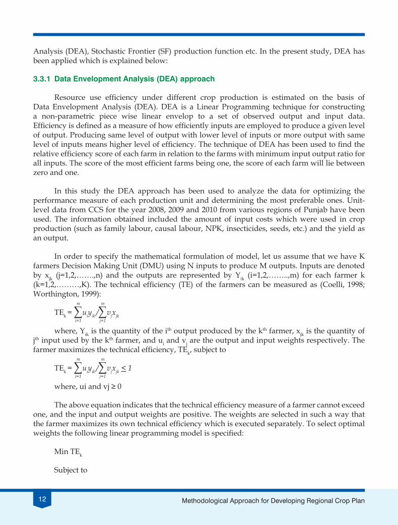
Analysis (DEA), Stochastic Frontier (SF) production function etc. In the present study, DEA has been applied which is explained below:
3.3.1 Data envelopment Analysis (DeA) approach
Resource use efficiency under different crop production is estimated on the basis of Data Envelopment Analysis (DEA). DEA is a Linear Programming technique for constructing a non-parametric piece wise linear envelop to a set of observed output and input data. Efficiency is defined as a measure of how efficiently inputs are employed to produce a given level of output. Producing same level of output with lower level of inputs or more output with same level of inputs means higher level of efficiency. The technique of DEA has been used to find the relative efficiency score of each farm in relation to the farms with minimum input output ratio for all inputs. The score of the most efficient farms being one, the score of each farm will lie between zero and one.
In this study the DEA approach has been used to analyze the data for optimizing the performance measure of each production unit and determining the most preferable ones. Unit-level data from CCS for the year 2008, 2009 and 2010 from various regions of Punjab have been used. The information obtained included the amount of input costs which were used in crop production (such as family labour, causal labour, NPK, insecticides, seeds, etc.) and the yield as an output.
In order to specify the mathematical formulation of model, let us assume that we have K farmers Decision Making Unit (DMU) using N inputs to produce M outputs. Inputs are denoted by xjk (j=1,2,…….,n) and the outputs are represented by Yik (i=1,2,……..,m) for each farmer k (k=1,2,………,K). The technical efficiency (TE) of the farmers can be measured as (Coelli, 1998; Worthington, 1999):
TEk = ∑m
i=1 uiyik /∑
m
j=1 vjxjk
where, Yik is the quantity of the ith output produced by the kth farmer, xjk is the quantity of jth input used by the kth farmer, and ui and vj are the output and input weights respectively. The farmer maximizes the technical efficiency, TEk, subject to
TEk = ∑m
i=1 uiyik /∑
m
j=1 vjxjk < 1
where, ui and vj ≥ 0
The above equation indicates that the technical efficiency measure of a farmer cannot exceed one, and the input and output weights are positive. The weights are selected in such a way that the farmer maximizes its own technical efficiency which is executed separately. To select optimal weights the following linear programming model is specified:
Min TEk
Subject to

13Methodological Approach for Developing Regional Crop Plan
∑m
i=1 ui yik ― yjk+w ≥ 0
where, k=1,2,……………,K
xjk― ∑n
j=1 ujxjk ≥ 0
and ui and vj ≥ 0
The above model shows TE under constant returns to scale (CRS) with an assumption if w = 0 and it changes into variable returns to scale (VRS) if w is used unconstrained. In the first case it leads to technical efficiency (TE) and in the second case pure technical efficiency (PTE) is estimated.
Technical Efficiency (TE) : It can be expressed generally as the ratio of sum of the weighted outputs to sum of weighted inputs. The value of technical efficiency varies between zero and one; where a value of one implies that the DMU is the best performer located on the production frontier and has no reduction potential. Any value of TE lower than one indicates that the DMU uses inputs inefficiently (Mousavi-Avval et. al., 2011).
Cost or Economic Efficiency (CE) : One can measure both technical and allocative efficiencies to verify the behavioral objectives such as cost minimization or revenue maximization.
Cost minimization DEA is expressed as
Min YXk* wk’ Xk*,
Subject to – yk +YY > 0,
Xk* - XY > 0,
Y > 0,
where wk’ is a vector of input prices for the kth farmer and Xk* (which is calculated by LP) is the cost minimizing vector of input quantities for the kth farmer, given the input prices wk and the output level yk. .
Total cost efficiency (CE) or economic efficiency of the kth farmer can be calculated as
CE = wk’Xk*/ wk’ Xk
That is the ratio of minimum cost to the observed cost.
While the allocative efficiency (AE) is calculated as the ratio of cost efficiency to technical efficiency
AE = CE / TE

14 Methodological Approach for Developing Regional Crop Plan
3.4 cOSt-RetURN ANALYSIS
The performance of different crops can be assessed by comparing net returns under alternative scenarios. These are: (i) Market prices; (ii) Economic prices net of subsidies; and (iii) Income based on natural resource valuation technique (Raju et.al. 2015). Overall framework is illustrated in figure 8. The computation of cost- returns using these three approaches has been explained with example of paddy crop in Punjab state for TE 2010-11 in the respective sections.
Figure 8 : Alternative ways to measure net returns of crops
3.4.1 Net returns at market prices (NR MP )
Net returns at market prices can be defined as the gross return (value of main product and by product) less variable costs (Cost A1 + imputed value of family labour) at market prices actually paid and received by the farmer or imputed in some cases.
NR MP = GR – VC …….. (i)
where, NR MP – Net return at market prices; GR- Gross Returns; and VC- Variable Cost.
This has been explained with an example given in table 3.
Table 3 : Computation of NR MP for paddy in Punjab during TE 2010-11, (Rs/ha)
Crop Gross returns (a)
Variable cost (Cost A1+FL)
(b)
Net returns at Market prices (NRMP)
(a-b)
Rice 69568 21885 47683
15Methodological Approach for Developing Regional Crop Plan
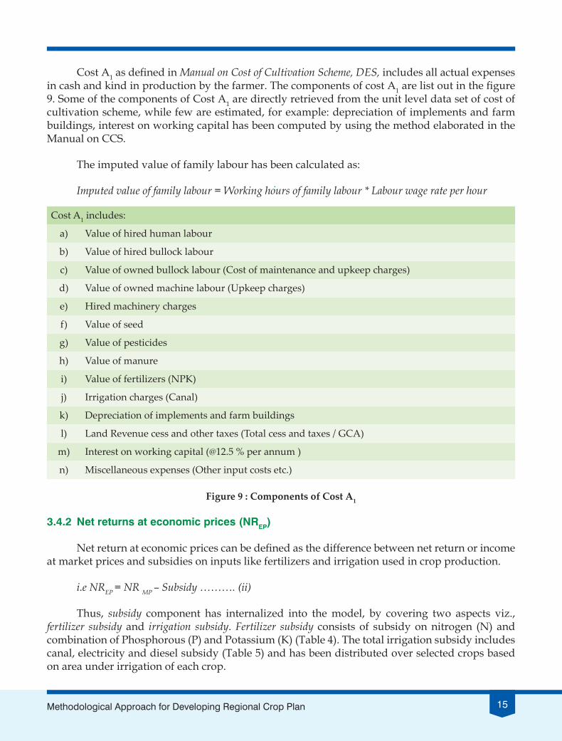
Cost A1 as defined in Manual on Cost of Cultivation Scheme, DES, includes all actual expenses in cash and kind in production by the farmer. The components of cost A1 are list out in the figure 9. Some of the components of Cost A1 are directly retrieved from the unit level data set of cost of cultivation scheme, while few are estimated, for example: depreciation of implements and farm buildings, interest on working capital has been computed by using the method elaborated in the Manual on CCS.
The imputed value of family labour has been calculated as:
Imputed value of family labour = Working hours of family labour * Labour wage rate per hour
Cost A1 includes:
a) Value of hired human labour
b) Value of hired bullock labour
c) Value of owned bullock labour (Cost of maintenance and upkeep charges)
d) Value of owned machine labour (Upkeep charges)
e) Hired machinery charges
f) Value of seed
g) Value of pesticides
h) Value of manure
i) Value of fertilizers (NPK)
j) Irrigation charges (Canal)
k) Depreciation of implements and farm buildings
l) Land Revenue cess and other taxes (Total cess and taxes / GCA)
m) Interest on working capital (@12.5 % per annum )
n) Miscellaneous expenses (Other input costs etc.)
Figure 9 : Components of Cost A1
3.4.2 Net returns at economic prices (NReP)
Net return at economic prices can be defined as the difference between net return or income at market prices and subsidies on inputs like fertilizers and irrigation used in crop production.
i.e NREP = NR MP – Subsidy ………. (ii)
Thus, subsidy component has internalized into the model, by covering two aspects viz., fertilizer subsidy and irrigation subsidy. Fertilizer subsidy consists of subsidy on nitrogen (N) and combination of Phosphorous (P) and Potassium (K) (Table 4). The total irrigation subsidy includes canal, electricity and diesel subsidy (Table 5) and has been distributed over selected crops based on area under irrigation of each crop.

16 Methodological Approach for Developing Regional Crop Plan
Table 4 : Computation of Fertilizer subsidy for paddy in Punjab during TE 2010-11
Paddy Use(kg/ha) (a)
Subsidy Rate(Rs/kg)* (b)
NPK Subsidy(Rs/ha) (a*b)
Nitrogen (N) 147 19.35 2843
Potassium (P) 4942.56
2067
Phosphorous (K) 42 1796
Total NPK 238 - 6705
Note: * Subsidy for P & K is in combination prior to Nutrient based subsidy policy, 2010
Crop wise irrigation subsidy has two components: Ground water subsidy and Surface water subsidy. Ground water subsidy can be estimated by initially calculating the crop-wise ground water use, i.e.
Groundwater use (cubic metre) = Irrigation hours (hrs/ha) * Groundwater draft (cum/hr)
The irrigation hours (hrs/ha) for each crop can be taken from plot-wise CCS data. CCS does not collect information of ground water draft. Therefore the groundwater draft can be estimated using the following formula:
Hp*75*Pump efficiencyGround water draft (lit/sec) = ―――――――――――――――― Total head (m)
The information on horse power (H P) of the pumps owned by the farmers is available in CCS data set. For the households purchasing groundwater, average HP of the pumps (estimated separately for electric and diesel) in respective tehsil can be taken as proxy. Pump efficiency is assumed to be 40 per cent. The total head can be obtained as per below equation:
Total head =Water level (mbgl*) + Draw down (m) + Friction loss (10% of water level+ Draw down)
The summation of groundwater draft from each category of pump-sets provides total groundwater-use (cum/ha) for each crop cultivated by the farmer. Further, the groundwater cost can be estimated separately for diesel pump, electric pump and submersible pump, by summing depreciation (tube-well and pump-set), interest (tube-well and pump-set) and upkeep costs. The subsidy per hectare of groundwater-use shall be estimated for electricpumps [product of per kilo-watt groundwater volume (cum/kWh) and subsidy rate (Rs/kWh)] and diesel pumps (product of diesel-use in extraction of groundwater and per litre subsidy rate during 2008-2011) separately (Srivastava et.al., 2015). Estimation of groundwater subsidy is illustrated in the table 5 by taking an example of paddy crop in Punjab for the TE 2010-11.
*Metres below ground level

17Methodological Approach for Developing Regional Crop Plan
Table 5: Estimation of Ground water extraction cost and ground water irrigation subsidy for paddy crop in Punjab during TE 2010-11
S.No. Items Diesel pump
Electric centrifugal
Electric submersible
Overall
a Irrigation Hours (hrs/ha) 11 124 150 285
b Power of the Pump (hp) 9 5 10
c Water Level (mbgl) 13.5 13.5 13.5
d Draw down# (m) 0 0 0
e Friction loss (%) (10% of water level) 1.4 1.4 1.4
f Total Head (m) {c+d+e} 14.9 14.9 18.9Υ
g Pump Efficiency (%) 0.4 0.4 0.4
h Groundwater draft (lit/sec) {(b*75*g)/f} 18.13 10.07 15.92
i Groundwater draft (cum/hr) {(h/1000)*3600} 65.26 36.26 57.29
j Total groundwater use (cum/ha) (i*a) 718 4496 8594 13808
k Depreciation of pumpsets and tubewells@ (Rs) 51 312 778 1141
l Interest on pumpset and tubewell (Rs) 92 163 1287 1542
m Upkeep cost (Rs)$ 571 86 140 797
n Total fixed cost +maintenance cost (Rs) {k+l+m} 714 561 2205 3480
o Fixed cost (Rs/cum) {n / j} 0.99 0.12 0.26 0.23
p Energy use {diesel (lit/cum) / electricity (kwh/cum)} € 0.02 0.10 0.13
q Groundwater subsidy (Rs/cum) {p*subsidy rateπ} 0.28 0.33 0.42 0.37
r Groundwater Subsidy (Rs/ha) {q * j} 203 1480 3581 5264
s Energy cost (Rs/cum) {p* unit rate of energyθ}
s1. Subsidized 0 0
s2. Unsubsidized 0.33 0.42
r Total groundwater cost (Rs/cum) r1. Subsidized {O+s1}
0.99 0.12 0.26 0.23
r2. Unsubsidized {r1+q}
1.28 0.45 0.67 0.60
Notes: # Drawn down in case of Punjab is assumed as 0 because of alluvial type aquifer Υ For submersible pumps additional depth of 4 metre was added to the total head because these pumps are placed far below the
groundwater table
@ Total depreciation and interest on groundwater structure and pump sets is allocated for paddy crop based on working hours of the pumps. The depreciation of hired pump-sets is also assumed to be similar to owned pump-sets
$ Upkeep cost for diesel pumps includes the cost of diesel € Energy use for electric pumps = (hp*0.746) / groundwater draft, where, 1 hp= 0.746 kwh; Energy use for diesel
pumps = (diesel use * Irrigation Hrs) /Total groundwater draft, where diesel use=1.43 lit/hr π Diesel subsidy @ Rs. 12.95 per litre and Electricity subsidy @ Rs. 3.20 per unit in TE 2010-11 respectively θ Unit rate of electricity: 3.20 per unit in TE 2010-11

18 Methodological Approach for Developing Regional Crop Plan
For estimating Surface / Canal water irrigation subsidy, data can be collected fromthe report on “financial aspects of irrigation projects in India” published by Central Water Commission. By summing over capital expenditure and working expenses on various irrigation projects viz., major, medium and minor irrigation projects, total expenditure can be worked out. Similarly gross receipts can be estimated for various canal irrigation projects in the state.
Gross subsidy can be calculated as follows:
Gross Subsidy = Total Expenditure - Gross Receipts
Gross subsidy is there after allocated across different crops in proportion to respective gross irrigated area. Illustration for computation of canal water irrigation subsidy has been elaborated in the table 6.
Table 6 : Estimation of canal water irrigation subsidy for paddy crop in Punjab during TE 2010-11
S.No. Items
a Expenditure on major, medium and minor projects (Rs lakhs) 101614
b Gross receipts (Rs lakhs) 2571
c Total subsidy (Rs lakhs) (a-b) 99043
d GIA by canal (‘000 ha) 2191
e Subsidy (Rs/GIA) {(c*100000)/(d*1000)} 4520
f Canal irrigated area under paddy (ha) 554
g Area under paddy crop (ha) 2364
h Subsidy total (Rs) (f * e) 2504080
i Canal water subsidy (Rs/ha) (h/g) 1059
After deriving the different subsidy components, Net return at economic prices (NREP) can be calculated by subtracting total subsidy from the value of net returns at market prices (NRMP) as shown in the table 7 for paddy crop in Punjab.
Table 7 : Computation of net returns at economic prices (NR EP) for paddy in Punjab during TE 2010-11, (Rs/ha)
Crop Irrigation Subsidy NPK subsidy
(c)
Total subsidy
(d=a+b+c)
Net returns at Market
prices (NR MP )
(e)
Net returns by economic
prices (NR EP ) (f = e-d)
Ground Water
(a)
Canal water
(b)
Paddy 5264 1059 6705 13028 47683 34658

19Methodological Approach for Developing Regional Crop Plan
3.4.3 Net returns based on natural resource valuation (NRNRV)
Net return based on Natural Resource Valuation (NRV) technique has taken care of nitrogen fixation by legume crops and Green House Gas (GHG) emission from crop production. As such NRNRV is computed as by adding value of nitrogen fixation by legume crops at economic price of nitrogen (Value of N) and deducting the imputed value of increase in GHG emission cost to the atmosphere.
i.e. NRNRV = NR EP + (Value of N– cost of GHG) ………. (iii)
Thus, legumes are environment-friendly crops and are different from other food plants because of the property of synthesizing atmospheric nitrogen into plant nutrients. As such, the economic valuation has been done by taking into account the positive externality of legume crops by biological nitrogen fixation and the negative externality of GHG emissions, as presented in the Appendix 1(a) to 1(d).
The data on contribution of pulses by biological nitrogen fixation and emission of of different crops were collected from various published scientific literature, (Peoples et al., 1995, IIPR, 2003, IARI, 2014).The value of GHG emissions in terms of CO2Kg equivalent was taken at the rate of 10 US dollar per tonne. Biological nitrogen fixation for various crops has been calculated by taking the average value of nitrogen fixed by various legumes and then multiplied with the economic price of nitrogen prevailed in the TE 2010-11.
Thus net return based on natural resource valuation (NRNRV) has taken into account the environmental benefits and has been illustrated in the table Table 8 for the case of paddy in Punjab.
Table 8: Computation of net returns based on NRV (NRNRV) for paddy in Punjab during TE 2010-11, (Rs/ha)
Crop Net Returns based on Economic Prices (NR EP)
(a)
Value of nitrogen
(b)
Cost of GHG emissions
(c)
Net returns based on NRV(NRNRV) (d) = (a)+(b)-(c)
Paddy 34658 0 1838 32820
3.5 OPtIMIzAtION Of cROP MODeL
The Mathematical Programming can be used for developing optimum crop or land use planning. It is an easy and flexible method for assessing different ways to use limited resources under variable objectives and constraints.
The present study makes an attempt to develop different crop planning strategies by using linear programming (LP). It develops the crop model which increases the productivity with minimum input cost under the constraints of available resources like water usage and also labour, fertilizers, seeds, etc., and ultimately getting maximum net benefits. Multi-crop model for two seasons are formulated in LP for maximizing the net returns, minimizing the cost and minimizing the water usage by keeping all other available resources (such as cultivable land, seeds, fertilizers, human labour, pesticides, capital etc.) as constraints.

20 Methodological Approach for Developing Regional Crop Plan
3.5.1Mathematicalspecificationsofthemodel
Mathematically, model specification for Punjab are presented by Equations 1-6 followed by equation wise description.
Max Z = ∑n
c=1 YcPc —Cc ) Ac (1)
∑
t ∑
c atc Ac < NSt —OAt (2)
Ac > A minc (3)
Ac < A maxc (4)
∑
c wc Ac < RGWAA (5)
Ac > 0 (6)
3.5.2 ObjectiveFunction:Maximizationofnetincome(Equation1)
∑
nc=1 (Yc Pc — Cc) Ac
Let Yc denotes yield of a crop c in one hectare of land, P the price received for the output from crop c, Cc refers to the cost incurred to cultivate crop c in one hectare of land and Ac is the area under cultivation of crop c then the RHS of the Equation 1 represents sum of net revenue obtained from all the crops considered for the optimum model development. The objective is to maximize the net revenue (z) based on the optimum crop plan.
Land Constraint
Optimum use of land for each month is required. This can be achieved by having separate constraint equation (Equation 2 is a compact form of 12 equations one for each month as shown below). This helps to have separate sown area for each month and ensures that total cultivated area under selected crops in each month should be less than net sown area (NSt) minus area under orchard (OAt)crops. Further crop calendar has to be maintained as per format in Figure 10 (Crop calendar for Punjab). Thus, atc in equation 2 refers to the coefficient of crop calendar matrix (Figure 10) for tth month and cth crop.
∑
c aJan c Ac < NSJan — OAJan
∑
c aFeb c Ac < NSFeb — OAFeb
∑
c aMar c Ac < NSMar — OAMar
∑
c aApr c Ac < NSApr — OAApr
∑
c aMay c Ac < NSMay — OAMay
∑
c aJun c Ac < NSJun — OAJun

21Methodological Approach for Developing Regional Crop Plan
∑
c aJul c Ac < NSJul — OAJul
∑
c aAug c Ac < NSAug — OAAug
∑
c aSep c Ac < NSSep — OASep
∑
c aOct c Ac < NSOct — OAOct
∑
c aNov c Ac < NSNov — OANov
∑
c aDec c Ac < NSDec — OADec
∑
t ∑
c atc Ac < NSt —OAt
3.5.3Minimumandmaximumconstraints(Equation3-4)
Crop planning model using LP primarily captures the supply side behavior specifically area response based on net returns and resource constraints ignoring the demand aspect. Such models tend to over-estimate or under-estimate the area allocations for some crops. As a consequence, a single crop may cover infeasible larger area (over-estimation) or null or negligible area (under-estimation).
In some modelling solutions, some major crops may drastically lose their relevance and the corresponding area allocations may become negligible. Then, even though estimates are robust and mathematically proven, such allocations may not be desirable and practically possible from the view point of food security of the country and livelihood security of the farmer because appropriate changes are required in policy framework of the country to adopt the optimum sustainable model. Similarly, area allocations for some minor crops may be over-estimated ignoring the demand. Such an area allocation is again undesirable as it may lead to glut in the market. To avoid such undesirable over-estimation or under-estimation, assigning values to minimum and maximum area of the selected crops become essential in the model. To eliminate such practically undesirable solutions, concept of min, max constraints is used in the model as specified by the equations 3-4.
3.5.4 ground water constraints
Water is a scarce natural resource. The ground water usage should be less than or equal to replenishable ground water available for agriculture (RGWAA) for making the agriculture sustainable. Data of RGWAA is published by Central Ground Water Board. RGWAA can be estimated by deducting water consumed by industries and other non-farm sectors from total replenishable ground water.
Ground water constraint to be used in linear programming (LP) model for Punjab agriculture is as follows:
∑
c wc Ac < RGWAA

22 Methodological Approach for Developing Regional Crop Plan
where wc is actual water drafted for a crop c in recent years based on Cost of Cultivation data. Ac refers to the area allocation for a crop c.
For the Punjab state, different scenarios have been developed by using different values of RGWAA e.g. (1) unlimited use of water by not using the water constraint, (2) sustainable water use (20 BCM) (Table 9). Data for development of RCP for Punjab has been taken from both secondary sources as well as household survey data from COC. However there can be some variations in other regions depending on the regional specific constraints and objective functions.
Existing land area allocations under different crops are useful to make comparison with optimum crop plan model. The data is available from statistical abstracts of Punjab. This data is further useful for defining minimum and maximum area allocation limits for the selected crops. Existing area is based on the three years average land use under the crops. Minimum and maximum area has been determined based on expert elicitation method.
sts
23Methodological Approach for Developing Regional Crop Plan
4OptimumCropModelforPunjab–ACaseStudy
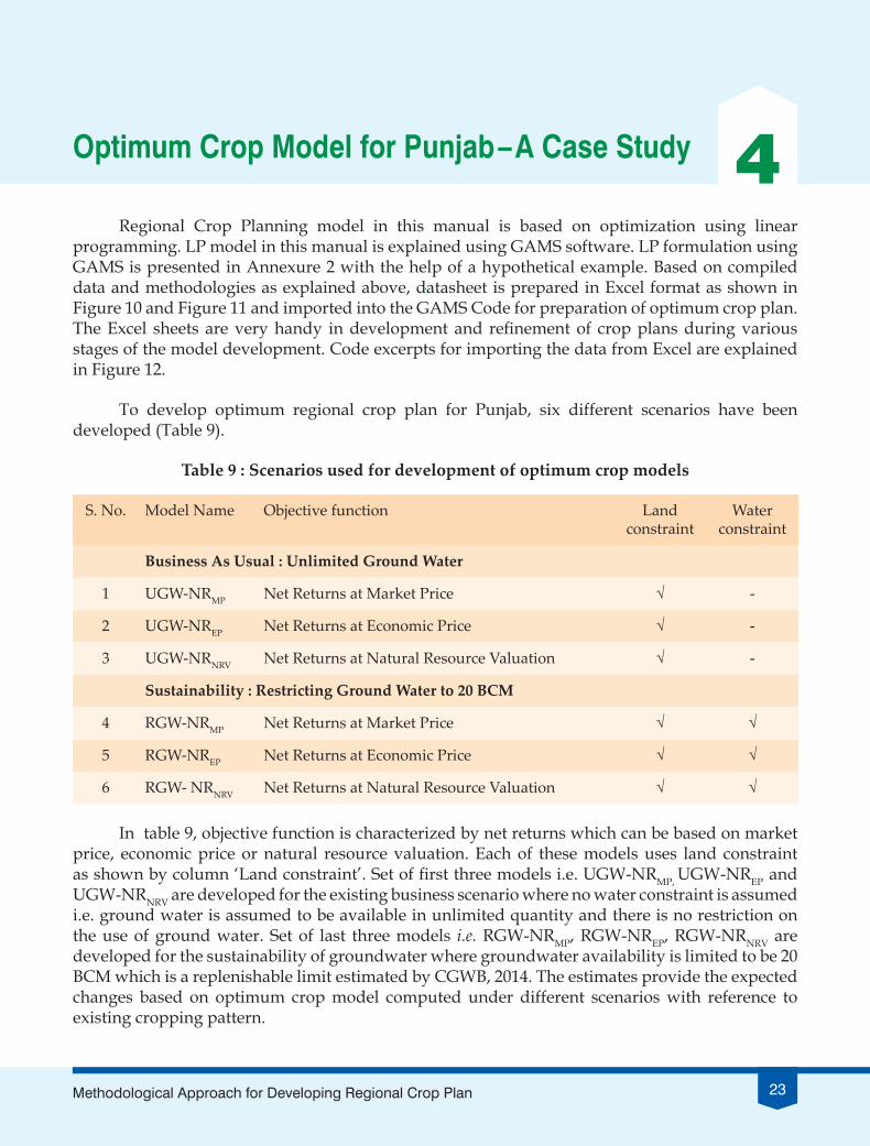
Regional Crop Planning model in this manual is based on optimization using linear programming. LP model in this manual is explained using GAMS software. LP formulation using GAMS is presented in Annexure 2 with the help of a hypothetical example. Based on compiled data and methodologies as explained above, datasheet is prepared in Excel format as shown in Figure 10 and Figure 11 and imported into the GAMS Code for preparation of optimum crop plan. The Excel sheets are very handy in development and refinement of crop plans during various stages of the model development. Code excerpts for importing the data from Excel are explained in Figure 12.
To develop optimum regional crop plan for Punjab, six different scenarios have been developed (Table 9).
Table 9 : Scenarios used for development of optimum crop models
S. No. Model Name Objective function Land constraint
Water constraint
Business As Usual : Unlimited Ground Water
1 UGW-NRMP Net Returns at Market Price √ -
2 UGW-NREP Net Returns at Economic Price √ -
3 UGW-NRNRV Net Returns at Natural Resource Valuation √ -
Sustainability : Restricting Ground Water to 20 BCM
4 RGW-NRMP Net Returns at Market Price √ √
5 RGW-NREP Net Returns at Economic Price √ √
6 RGW- NRNRV Net Returns at Natural Resource Valuation √ √
In table 9, objective function is characterized by net returns which can be based on market price, economic price or natural resource valuation. Each of these models uses land constraint as shown by column ‘Land constraint’. Set of first three models i.e. UGW-NRMP, UGW-NREP and UGW-NRNRV are developed for the existing business scenario where no water constraint is assumed i.e. ground water is assumed to be available in unlimited quantity and there is no restriction on the use of ground water. Set of last three models i.e. RGW-NRMP, RGW-NREP, RGW-NRNRV are developed for the sustainability of groundwater where groundwater availability is limited to be 20 BCM which is a replenishable limit estimated by CGWB, 2014. The estimates provide the expected changes based on optimum crop model computed under different scenarios with reference to existing cropping pattern.

24 Methodological Approach for Developing Regional Crop Plan
Figure 10 : Excel sheet named ‘data’ for showing crop calendar for selected crops
Figure 11 : Excel sheet named ‘limit’ for data inputs to GAMS program

25Methodological Approach for Developing Regional Crop Plan
*setting working directory *$setglobal path “J:\RCPModel1\”
*Sets command is used to Define Object which consist of elements (usually names)**This facilitate vector or matrix computation by working like index items**C is Set or group of object, labelled as “crops”, consists of many element -crop names**C is imported (not imputed directly as in the other set)**call=xls2gms.exe command is used to import crop names from Excel file “specified input location: I “ **to “specified output location :O" as include file* and the range specified by R:*$include %path%regional_LP.inc command is used to include data into gams running environment from specified file *Sets c crops/$call =xls2gms.exe I=%path%regional_LP.xls O=%path%regional_LP.inc R=limit!a2:a26$include %path%regional_LP.inc/ ;
*display command used to display the set or objects**Here it is used to check whether object has been created or not *display “crops List”, c;
*Group of object “t” defined using set command and labelled as period **Object “t” consist of elements - month names**Group of object “st” defined using set command and labelled as stat **Object “st” consist of elements like “area”, “minA” and etc: names of variables**Set command part has to be terminated with semicolon*set t period /jan,feb,mar,apr,may,jun,jul,aug,sep,oct,nov,dec/st stat /area,minA,MaxA,Nreturn,water,EcoPrice,NRV/ ;
*parameter are defined and used to import data (usually numeric)**Precaution: Here name of crops should match in the same order in both Excel files set c and land(t,c)*parameter land is imported in two steps**First step : using gdxxrw.exe data are converted from Excel file to gdx format “** initiate the command of GDXIN to read/accessed gdx format data by gams**load the data in to “land”** stop GDXINparameter land(t,c) ;$call gdxxrw.exe %path%regional_LP.xls par=land rng=data!a1:z13$GDXIN %path%regional_LP.gdx$load land$GDXINdisplay land;
*parameter “Arealmt” is defined and displayed *
Figure 12 : GAMS code for developing RCP with code description

26 Methodological Approach for Developing Regional Crop Plan
parameter Arealmt (c,st) ;$call gdxxrw.exe %path%regional_LP.xls par=Arealmtrng=limit!a1:h26$GDXIN %path%regional_LP.gdx$load Arealmt$GDXINdisplay Arealmt;
*new parameters are defined and explained by respective labels*PARAMETERNR (c) net revenue per haAR (c) Existing Area in hajal(c) water requirement per hectare cubic metermnA(c) Minimum limit of area in hamxA(c) Maximum limit of area in ha;
*newly defined parameters are populated by the values from the Arealmt parameter*NR(c)= Arealmt(c,”NRV”) ;AR (c)= Arealmt (c,”area”) ;jal(c)= Arealmt(c,”water”) ;mnA (c)= Arealmt(c,”MinA”) ;mxA (c)= Arealmt(c,”MaxA”) ;display NR;display AR;display jal;display mnA;display mxA;
*Scalars are defined and inputted directly**scalars are single value constants**nca Net sown area in Thousand Ha*/*gwa total ground water available in Billion Cubic Meter (BCM) /20/Scalarsnca Net sown area in Thousand Ha /4000 /gwa total ground water available in Billion Cubic Meter (BCM) /20/
*Variables are endogenous variables**positive variables are nonnegative endogenous variables**Equations command is used to declare Names of equations that will appear in the models*
variablesprof profit (in RS)carea (c) quantity (in hectares)positive variablescarea (c)Equationslandeq (t) land allocationminArea (c) Minimum area restrictionmaxArea (c) Maximum area restriction

27Methodological Approach for Developing Regional Crop Plan
waterc water constraintprofit profit form production;
*/ landeq (t): area under cultivation will be limited by total cropped area in each monthlandeq (t).. sum(c, carea(c)*land(t,c)*1000) =l= nca*1000;
*/ minimum area under each crop is constrained by the userminArea (c).. carea(c)*1000 =g= mnA(c)*1000 ;
*/ maximum area under each crop is constrained by the usermaxArea (c).. carea(c)*1000 =l= mxA(c)*1000 ;
*Ground water use across the crops should be subject to availability of ground water availability*waterc.. sum(c, jal(c)*carea(c)*1000) =l= gwa*1000000000*Aag;
*Profitability is sum of net return from optimized regional crop plan*profit.. prof =e= sum(c, NR(c)*carea(c)*1000);
*Model consist of set of equation, to be solved *Model regional regional crop production /all/;
*Executing the solver using linear programming **lp is a solver module**objective is to maximize the profit under given set of constraints*
solve regional using lp maximizing prof
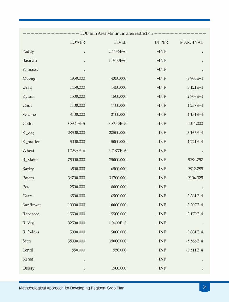
For expounding purpose, business as usual scenario result is presented for market price (UGW-NRMP) in detail using GAMS solve summary which is output of GAMS program (Figure 13). First part of the output shows the model statistics and summary of the model followed by objective function value. Second part shows the equation solution report and the third part presents variable solution report (Figure 13). Similarly GAMS solve summary can be obtained for other models of Table 9. Variable solution report from each of the GAMS solve summary of all these models has been used for consolidation of results, comparing net returns, GCA change and gains from the optimum model (Table 10-12, Figure 13).
Table 10 shows Optimum area allocations for Kharif and Rabi season crops separately for different prices and unlimited water availability scenarios (UGW-NRMP, UGW-NREP, UGW-NRNRV). It is observed that cropping pattern is similar in all the three price scenarios (Table 10). On comparing the optimum pattern with existing cropping pattern, it is to be noted that during Kharif, paddy area tends to further increase in all three price scenarios (Table 10). Area under wheat and vegetables show increase in cropped area under all three scenarios.

28 Methodological Approach for Developing Regional Crop Plan
Table 10 : Optimum crop model for unrestricted GW use : Business as usual scenario
Crops Existing area (000 ha)
Optimum area (000 ha) Direction of Change
Market Price
Economic Price
Natural Resource Valuation
Kharif Season
Paddy (including Basmati) 2760.0 3523.6 3523.6 3523.6 + + +
Maize 136.0 0 0 0 _ _ _
Cotton 483.0 386.4 386.4 386.4 _ _ _
Vegetables 57.0 28.5 28.5 28.5 _ _ _
Others (including fodder) 28.0 16.5 16.5 16.5 _ _ _
Rabi Season
Wheat 3519.7 3707.8 3706.3 3706.3 + + +
Maize 150.0 75.0 75.0 75.0 _ _ _
Vegetables 65.0 104.0 104.0 104.0 + + +
Potato 69.4 34.7 34.7 34.7 _ _ _
Oilseeds (Rapeseed+Sunflower) 51.0 25.5 25.5 25.5 _ _ _
Others (including fodder) 39.1 28.1 29.6 29.6 _ _ _
Sugarcane 70.0 35.0 35.0 35.0 _ _ _
Gross Cropped Area 7428.2 7965.0 7965.0 7965.0 + + +
Table 11 shows optimum area allocations for Kharif and Rabi season crops separately for different prices and water availability restricted to 20 BCM scenarios represented by the models RGW-NRMP, RGW-NREP and RGW-NRNRV.
In Table 11, it is observed that cropping pattern is similar in all three price scenarios. On comparing the optimum pattern with existing cropping pattern, it is observed that during Kharif, paddy, vegetables and other crops area tends to decrease in all three price scenarios while maize and cotton area tends to increase (Table 11). In Rabi season, wheat and vegetables show increase in cropped area but all other crops show decrease in the respective cropped area.

29Methodological Approach for Developing Regional Crop Plan
Table 11 : Optimum crop model for GW use restricted to 20 BCM : Ground water sustainability scenario
Crops Existing area (000 ha)
Optimum area (000 ha) Direction of ChangeMarket
PriceEconomic
PriceNatural
Resource Valuation
Kharif Season
Paddy (including Basmati) 2760.0 724.0 729.8 729.8 _ _ _
Maize 136.0 217.6 217.6 217.6 + + +
Cotton 483.0 579.6 579.6 579.6 + + +
Vegetables 57.0 28.5 28.5 28.5 _ _ _
Others (including fodder) 28.0 29.1 19.5 19.5 _ _ _
Rabi Season
Wheat 3519.7 3707.8 3707.8 3707.8 + + +
Maize 150.0 150.0 75.0 75.0 _ _ _
Vegetables 65.0 104.0 104.0 104.0 + + +
Potato 69.4 34.7 34.7 34.7 _ _ _
Oilseeds(Rapeseed+Sunflower) 51.0 47.5 25.5 25.5 _ _ _
Others(including fodder) 39.1 28.1 28.1 28.1 _ _ _
Sugarcane 70.0 35.0 35.0 35.0 _ _ _
Gross Cropped Area 7428.2 5610.8 5585.0 5585.0 _ _ _
Expected changes based on optimum crop model estimated under different price and water scenarios with reference to existing cropping pattern are presented in Table 12.
Table 12: Gains due to optimum crop model over existing scenario
Optimum Scenario (1) Change in GCA %
(2)
Existing Revenue
(00 Crores)
(3)
Optimal Net
Returns (00
Crores) (4)
Change in Farmer Revenue
(00 Crores) (Optimal -
Existing MP ) (5)
Gain to society
(00 crore)
(6)
Net Gain (00 crore)
(7)=(5)+(6)Unrestricted water use
Market Price 7.2 297.3 332.0 34.7 - 34.7Economic Price 7.2 213.5 240.8 -56.5 83.8 27.3Natural Resource Valuation 7.2 207.7 233.6 -63.7 78 14.3
Sustainable water use (20 BCM)Market Price -24.5 NA 211.4 -85.9 NA NAEconomic Price -24.8 NA 152.1 -145.2 NA NANatural Resource Valuation -24.8 NA 150.0 -147.3 NA NA

30 Methodological Approach for Developing Regional Crop Plan
SOLVE SUMMARYFirst Part
MODEL regionalN_MP OBJECTIVE profTYPE LP DIRECTION MAXIMIZESOLVER CPLEX FROM LINE 201
**** SOLVER STATUS 1 Normal Completion **** MODEL STATUS 1 Optimal **** OBJECTIVE VALUE 332019607401.4761
RESOURCE USAGE, LIMIT 0.015 1000.000ITERATION COUNT, LIMIT 1 2000000000
IBM ILOG CPLEX 24.3.3 r48116 Released Sep 19, 2014 WEI x86 64bit/MS Windows Cplex 12.6.0.1
Space for names approximately 0.00 MbUse option ‘names no’ to turn use of names offLP status(1): optimalCplex Time: 0.00sec (det. 0.07 ticks)Optimal solution found.Objective : 332019607401.476070
Second Part
————————————————— EQU landeq land allocaton ————————————————
LOWER LEVEL UPPER MARGINAL
Jan -INF 4.0000E+6 4.0000E+6 .
Feb -INF 4.0000E+6 4.0000E+6 .
Mar -INF 4.0000E+6 4.0000E+6 .
Apr -INF 3.8293E+6 4.0000E+6 .
May -INF 4.2140E+5 4.0000E+6 .
Jun -INF 3.9957E+6 4.0000E+6 .
Jul -INF 4.0000E+6 4.0000E+6 .
Aug -INF 4.0000E+6 4.0000E+6 .
Sep -INF 4.0000E+6 4.0000E+6 46198.000
Oct -INF 2.3507E+6 4.0000E+6 .
Nov -INF 4.4470E+5 4.0000E+6 .
Dec -INF 4.0000E+6 4.0000E+6 36244.325
Figure 13 : GAMS solve summary
31Methodological Approach for Developing Regional Crop Plan
—————————————— EQU min Area Minimum area restriction —————————————
LOWER LEVEL UPPER MARGINAL
Paddy . 2.4486E+6 +INF .
Basmati . 1.0750E+6 +INF .
K_maize . . +INF .
Moong 4350.000 4350.000 +INF -3.906E+4
Urad 1450.000 1450.000 +INF -5.121E+4
Rgram 1500.000 1500.000 +INF -2.707E+4
Gnut 1100.000 1100.000 +INF -4.258E+4
Sesame 3100.000 3100.000 +INF -4.151E+4
Cotton 3.8640E+5 3.8640E+5 +INF -4011.000
K_veg 28500.000 28500.000 +INF -3.166E+4
K_fodder 5000.000 5000.000 +INF -4.221E+4
Wheat 1.7598E+6 3.7077E+6 +INF .
R_Maize 75000.000 75000.000 +INF -5284.757
Barley 6500.000 6500.000 +INF -9812.785
Potato 34700.000 34700.000 +INF -9106.325
Pea 2500.000 8000.000 +INF .
Gram 6500.000 6500.000 +INF -3.361E+4
Sunflower 10000.000 10000.000 +INF -3.207E+4
Rapeseed 15500.000 15500.000 +INF -2.179E+4
R_Veg 32500.000 1.0400E+5 +INF .
R_fodder 5000.000 5000.000 +INF -2.881E+4
Scan 35000.000 35000.000 +INF -5.566E+4
Lentil 550.000 550.000 +INF -2.511E+4
Kenaf . . +INF .
Oelery . 1500.000 +INF .

32 Methodological Approach for Developing Regional Crop Plan
————————————— EQU Max Area Maximum area restriction —————————————
LOWER LEVEL UPPER MARGINAL
Paddy -INF 2.4486E+6 3.0400E+6 .
Basmati -INF 1.0750E+6 1.0750E+6 7178.793
K_maize -INF . 2.1760E+5 .
Moong -INF 4350.000 13920.000 .
Urad -INF 1450.000 4640.000 .
Rgram -INF 1500.000 4500.000 .
Gnut -INF 1100.000 3520.000 .
Sesame -INF 3100.000 9920.000 .
Cotton -INF 3.8640E+5 5.7960E+5 .
K_veg -INF 28500.000 91200.000 .
K_fodder -INF 5000.000 7500.000 .
Wheat -INF 3.7077E+6 4.1000E+6 .
R_Maize -INF 75000.000 2.4000E+5 .
Barley -INF 6500.000 20800.000 .
Potato -INF 34700.000 1.1104E+5 .
Pea -INF 8000.000 8000.000 8304.675
Gram -INF 6500.000 20800.000 .
Sunflower -INF 10000.000 32000.000 .
Rapeseed -INF 15500.000 49600.000 .
R_Veg -INF 1.0400E+5 1.0400E+5 12705.793
R_fodder -INF 5000.000 10000.000 .
Scan -INF 35000.000 1.1200E+5 .
Lentil -INF 550.000 1760.000 .
Kenaf -INF . 1500.000 .
Oelery -INF 1500.000 1500.000 18401.437

33Methodological Approach for Developing Regional Crop Plan
LOWER LEVEL UPPER MARGINAL—— EQU profit MP . . . 1.000 profit MP profit form production
Third Part
LOWER LEVEL UPPER MARGINAL—— VAR prof -INF 3.320E+11 +INF . prof profit (in RS)
—— VAR carea quantity (in hectares) LOWER LEVEL UPPER MARGINALPaddy . 2448.600 +INF . Basmati . 1075.000 +INF . K_maize . . +INF -3.387E+7 Moong . 4.350 +INF . Urad . 1.450 +INF . Rgram . 1.500 +INF . Gnut . 1.100 +INF . Sesame . 3.100 +INF . Cotton . 386.400 +INF . K_veg . 28.500 +INF . K_fodder . 5.000 +INF . Wheat . 3707.750 +INF . R_Maize . 75.000 +INF . Barley . 6.500 +INF . Potato . 34.700 +INF . Pea . 8.000 +INF . Gram . 6.500 +INF . Sunflower . 10.000 +INF . Rapeseed . 15.500 +INF . R_Veg . 104.000 +INF . R_fodder . 5.000 +INF . Scan . 35.000 +INF . Lentil . 0.550 +INF . Kenaf . . +INF -2.684E+6 Oelery . 1.500 +INF .
**** REPORT SUMMARY : 0 NONOPT 0 INFEASIBLE 0 UNBOUNDED

34 Methodological Approach for Developing Regional Crop Plan
The results pinpoint that unrestricted ground water use will further tend to increase the gross cropped area by 7 per cent while restricting the ground water use to replenishable limit of 20 BCM will tend to reduce the gross cropped area by 25 per cent. Optimal net returns are found to be relatively large with unrestricted ground water use while relatively low with restricted ground water use which decreases the cropped area under the water intensive crops. Further, optimal returns are found to be larger with market price and tend to decrease with economic price and natural resource valuation. Largest optimal net returns are observed in UGW-NRMP while smallest net returns are observed in RGW-NRNRV. Changes in farmers’ revenue from each of six models are estimated by subtracting the corresponding optimal model revenue from the existing revenue at market price. For example in Table 12, gains in farmers’ revenue at economic price (UGW-NREP) are estimated by subtracting optimal revenue of the model UGW-NREP from existing revenue of the model UGW-NRMP. This revenue change was found positive only in UGW-NRMP. However, this positive change is at the cost which is paid by the society in terms of declining water table and cost of subsidy on fertilizers, diesel, water and electricity. All other models show the negative change in farmer revenues. But there are positive gains to society. These gains are not estimated for sustainable water use scenario, because of the problems of estimation of cost of water saved. Finally net gains are estimated by adding changes in farmers’ revenue and gains to society. It is observed that net gains are positive in all the three model of business as usual scenario. The comparative results of the two scenarios show that it is difficult to shift to sustainable ground water use because of negative change in farmers’ revenue due to decrease in GCA. However, gradual decrease in ground water use is recommended which should be further supplemented by increasing ground water use efficiency, better package of practice for water intensive crops e.g. SRI cultivation, direct seeding for paddy cultivation.
sts
35Methodological Approach for Developing Regional Crop Plan
References
Chand, Ramesh; Sonia Chauhan, (2002), Socio Economic Factors in Agricultural Diversification in India, Agricultural Situation in India, February.
CGWB (2013), Master Plan for Artificial Recharge to Groundwater in India, Central Groundwater Board, Ministry of Water Resources, Government of India. http://cgwb.gov.in/documents/MasterPlan-2013.pdf.
CGWB (2014), Dynamic Groundwater Resources of India (As on 31st march, 2011), Central Groundwater Board, Ministry of Water Resources, River Development and Ganga Rejuvenation, Government of India, Faridabad.
Coelli, T. (1998), A Multi-Stage Methodology for the Solution of Orientated DEA Models, Operation Research Letters, Volume- 23(3-5): 143-149.
CWC (Central Water Commission) (various issues), Report on Financial Aspects of Irrigation Projects in India. Information technology directorate information system organization, Water planning and projects wing.
DES (Directorate of Economics and Statistics), Manual on Cost of Cultivation Surveys, Department of Agriculture, Government of India, available at http://mospi.nic.in/Mospi_New/upload/manual_cost_cultivation_surveys_23july08.pdf
GoI (Government of India) (2011) Central Ground Water Board, Ministry of Water Resources, New Delhi, available at: http://cgwb.gov.in/
GoI (Government of India) (various issues), Annual Report of Ministry of Chemicals and Fertilizers, Department of Fertilizers, New Delhi
GoPb (Government of Punjab) (2011), Report on Environment Statistics of Punjab, Economic and Statistical Organisation, Chandigarh.
GoPb (Government of Punjab) (various issues), Statistical Abstracts of Punjab, Chandigarh.
GoPb (Government of Punjab), Punjab State Electricity Regulatory Commission, available at: http://www.pserc.nic.in/
IARI (Indian Agricultural Research Institute) (2014), GHG Emission from Indian Agriculture: Trends, Mitigation and Policy Needs. Centre for Environment Science and Climate Resilient Agriculture, pp.16.
IIPR (Indian Institute of Pulses Research) (2003), Pulses in new perspective, In Proceedings of the National Symposium on Crop Diversification and Natural Resource Management, Kanpur. pp. 20 – 22.
Mousavi-Avval SH, Rafiee S., Jafari A, Mohammadi A. (2011), Optimization of energy consumption for soybean production using Data Envelopment Analysis (DEA) approach. Applied Energy. 35: 2156-2164.

36 Methodological Approach for Developing Regional Crop Plan
Pal, Swades and Kar, Shyamal (2012), Implications of the methods of agricultural diversification in reference with Malda district: drawback and rationale, International Journal of Food, Agriculture and Veterinary Sciences 2 (2): 97-105.
Peoples, M. B., Ladha, J. K. and Herridge, D. F. (1995), Enhancing legume N2 fixation through plant and soil management. Developments in Plant and Soil Sciences, 174: 83-101.
Raju, S.S., Ramesh Chand, S. K. Srivastava, Amrit Pal Kaur, Jaspal Singh, Rajni Jain, Kingsly Immaneulraj and Parminder Kaur (2015), Comparing Performance of Various Crops in Punjab Based on Market and Economic Prices and Natural Resource Accounting, Agricultural Economics Research Review, 28 (Conference issue).
Ramachandra, T.V. and Shwetmala, (2012), Decentralized carbon foot print analysis for opting climate change mitigation strategies in India, Renewable and Sustainable Energy Reviews, 16 (8): 5820-5833.
Srivastava, S.K., Ramesh Chand, S.S. Raju, Rajni Jain, Kingsly I., Jatinder Sachdeva, Jaspal Singh and Amrit Pal Kaur (2015), Unsustainable Groundwater Use in Punjab Agriculture: Insights from Cost of Cultivation Survey, Indian Journal of Agricultural Economics, 70 (Conference issue).
Worthington AC (1999), Measuring Technical Efficiency in Australian Credit Unions, Manchester School 67(2): 231-248.
sts

37Methodological Approach for Developing Regional Crop Plan
Annexure
ecONOMIc VALUAtION Of NItROgeN fIxAtION AND ghg eMISSION BY VARIOUS cROPS
(a) Estimatesofnitrogenfixedbylegumes(Kg/ha)
Crop Source I Source II Source III
Chickpea 23-97 26-63 120-140 Red gram 4-200 68-200 150 Green gram 50-66 50-55 112 Black gram 119-140 - 55-72 Cow Pea 9-125 53-85 47-188 Soybean 19-450 49-130 93-138 Cluster bean 37-196 37-196 - Pea 46 46 - Ground nut - 112-152 240-260
Source : I. Peoples et al., (1995); II . IIPR (2003); III. Residual effects of legumes in Rice-Wheat Cropping systems Pg. No. 109.
(b) Economiccontributionoflegumesthroughnitrogenfixation(Rs/ha)
S. No. Crop Contribution
1 Soybean 3865 2 Black gram 2506 3 Cluster bean 3533 4 Red gram 3412 5 Cowpea 3110 6 Lentil 1993 7 Green gram 2235 8 Chickpea 3140 9 Peas 1389 10 Groundnut 4560 11 Lucerne 4952 12 Stylo 3322
Source: Calculated by using Peoples et al., (1995) and IIPR (2003)
1

38 Methodological Approach for Developing Regional Crop Plan
(c) Methaneemissionfactorsforpaddycultivation
State Integrated Seasonal Methane Flux (g/m2)
Global Warming Potential (Kg CO2
equivalents per hectare)
GHG cost (Rs /ha)
Punjab 18.9 3969 1838Bihar 18.9 3969 1838Maharashtra 11.6 2436 1128Karnataka 11.0 2310 1070Tamil Nadu 11.0 2310 1070Rajasthan 11.6 2436 1128Assam 46.0 9660 4475
Note: Cost is calculated @10 USD per tonne of CO2 equivalents.Source: Ramachandra, T.V. and Shwetmala, (2012).
(d) GreenHouseGas(GHG)emissionfromselectedcropsinIndia
Crop CO2equivalent (Kg/Ha ) (Global Warming Potential)
GHG Cost (Rs/ha)
Wheat 340-450 157-208Maize 320-365 148-169Millets 230-250 107-116Oilseeds 220-275 102-127Pulses 180-240 83-111Vegetables 440-575 204-266
Note: Cost is calculated @10 USD per tonne of CO2 equivalents.Source: Calculated by using IARI (2014).
sts
39Methodological Approach for Developing Regional Crop Plan
Annexure 2gAMS BASIcS fOR SOLVINg cONStRAINeD OPtIMIzAtION PROBLeMS
This appendix is a ready reckoner for the beginners in GAMS. It explains the GAMS software and basic features of a GAMS program with the help of a small example. Further it also explains the interpretation and analysis of the GAMS output.
A2.1 ORIgIN Of gAMS SOftwARe
The GAMS software (General Algebraic Modelling System) was originally developed by a group of economists from the World Bank in order to facilitate the resolution of large and complex non-linear models on personal computer. As a matter of fact, GAMS allows solving simultaneous non-linear equation system, with or without optimization of some objective function. (i) Simplicity of implementation, (ii) portability and transferability between users and systems and (iii) easiness of technical update because of the constant inclusion of new algorithms are the main advantages of GAMS. The seminal GAMS system was file oriented. The program must be created in ASCII format with any one of the usual text editor run by a DOS command. The development of GAMS-IDE interface in the late 1990s makes it even easier to use. GAMS-IDE works as a general text editor compatible with WINDOWS and offers the ability to launch and monitor the compilation and execution of typical GAMS programs. In this introduction note we will present the general structure of the GAMS program, followed by a detailed illustration, including a description of the output file.
A2.2 hOw tO StARt gAMS
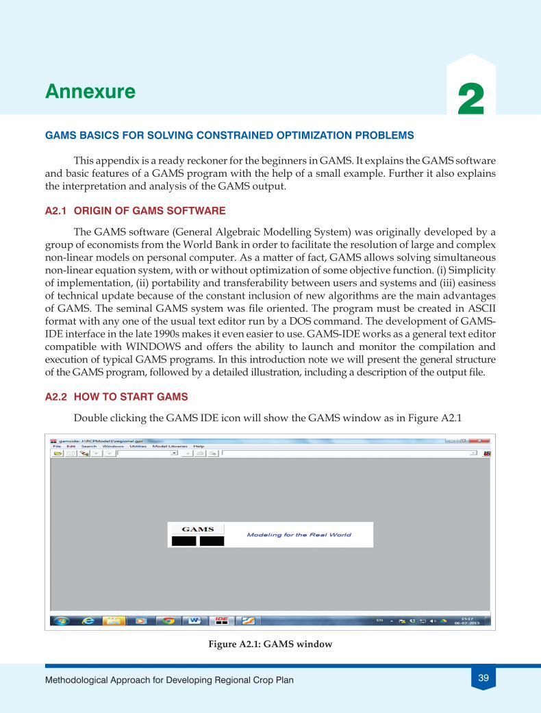
Double clicking the GAMS IDE icon will show the GAMS window as in Figure A2.1
Figure A2.1: GAMS window

40 Methodological Approach for Developing Regional Crop Plan
A2.3 hOw tO StARt A New PROJect
Once, IDE window opened, go to File à Project à New Project (Figure 2).
Figure A2.3: Opening a new project
Figure A2.2: Creating a new project
New window will open. Let us call our working folder name as optimization. Indicate this folder (Optimization) for working directory and give new name (here GAMS newproject) for newly created project file. Then click open (Figure A2. 3).

41Methodological Approach for Developing Regional Crop Plan
Then go to file menu à click new à click open (Figure A2. 4). New untitled.gms file will open (Figure A2. 5).
Figure A2. 4: Opening a new GAMS code file
Figure A2. 5: New untitled GAMS file

42 Methodological Approach for Developing Regional Crop Plan
A2.4 hOw tO wRIte gAMS cODe
GAMS program can be written in two different styles. (1) Without algebraic form (2) With algebraic form. The former forms are useful for beginner to understand the formulation each equation basis. It is suitable for small optimization problem and explanatory purpose. Later form is useful for larger optimization problem. Here text book equations can be easily translated in to problem formulation. It reduces the writing program time. It is suitable for experienced programmer.
gAMS Program Structure (without algebraic language)VariablesEquationsModelSolve
gAMS Program Structure (with algebraic language)SetData entry (Scalar, Parameter and Table)VariablesEquationsModelSolve
example
Max 109* Xcorn + 90* X wheat + 115* X Cottons.t. Xcorn + X wheat + X Cotton ≤ 100 (land) 6* Xcorn + 4* X wheat + 8* X Cotton ≤ 500 (land) Xcorn X wheat X Cotton ≥ 0 (non negativity)
LPformulationinGAMS(Withoutalgebraiclanguage)
VARIABLES Z;POSITIVE VARIABLES Xcorn, Xwheat, Xcotton;EQUATIONS OBJ, land, labor;OBJ.. Z=E=109* Xcorn + 90* Xwheat + 115* Xcotton;land.. Xcorn + Xwheat + Xcotton =L= 100;labor.. 6* Xcorn+ 4* Xwheat + 8* Xcotton = L=500;MODEL farm PROBLEM /ALL/;SOLVE farm PROBLEM USING LP MAXIMIZING Z;
explanation
VARIABLES Z;POSITIVE VARIABLES Xcorn, Xwheat, Xcotton;Variables : list of variable in model can assume both positive and negative valuesPositive variables : list of variable in model can assume only positive valuesNon Negative Variables : list of variable can assume zero or positive values.

43Methodological Approach for Developing Regional Crop Plan
Equations
GAMS requires that the modeler name each equation, which is active in the optimization model. Later each equation is specified using the notation as explained just below. These equations must be named in an EQUAT ION or EQUATIONS instruction. This is used in each of the example models as reproduced below.
EQUATIONS OBJ, land, labor;
OBJ.. Z =E= 109 * Xcorn + 90 * Xwheat + 115 * Xcotton;
land.. Xcorn + Xwheat + Xcotton =L= 100;
labor.. 6*Xcorn+ 4 * Xwheat + 8 * Xcotton =L= 500;
Equationspecification
The GAMS equation specifications actually consist of two parts.
The first part naming equations was discussed just above.
The second part involves specifying the exact algebraic structure of equations. This is done using the notation. In this notation we give the equation name followed by a then the exact equation type as it should appear in the model. The equation type specification involves use of a special syntax to tell the exact form of the relation involved. The most common of these are (see the Variables, Equations, Models and Solves chapter for a complete list ):
=E= is used to indicate an equality relation
=L= indicates a less than or equal to relation
=G= indicates a greater than or equal to relation
Model
Once all the model structural elements have been defined then one employs a MODEL statement to identify models that will be solved. Such statements are as follows in the given example.
MODEL farm PROBLEM /ALL/;
In the Model Statement in the model contents field
Using /ALL/ includes all the equations.
One can list equations in the model statement like that below.
MODEL FARM /obj, Land, labor/;
Naming Equation
Equation Specification

44 Methodological Approach for Developing Regional Crop Plan
Solve
Once one believes that the model is ready in such that it makes sense to find a solution for the variables then the solve statement comes into play. The SOLVE statement causes GAMS to use a solver to optimize the model or solve the embodied system of equations.
SOLVE farm PROBLEM USING LP MAXIMIZING Z;
Solve model name using model type; where Solve is required. A model name follows that must have already been given this name in a Model statement using is required. The model type is one of the known GAMS model types LP.
LinearProgrammingformulation(Withalgebraiclanguage)
Max Σj Cj Xj
s.t. Σj aij Xj ≤ bi for all i
Xj ≥ 0 for all j
where j = { com wheat cotton } i = { land labor } xj = { Xcorn Xwheat Xcotton } Cj = { 109 90 115 } aij = 1 1 1 6 4 8 bi = { 100 500 }'
SET j /Corn, Wheat, Cotton/i /Land, Labor/;
PARAMETERc(j) / corn 109, wheat 90, cotton 115/b(i) /land 100, labor 500/;
TABLE a(i,j)land 1 1 1labor 6 4 8 ;POSITIVE VARIABLES x(j);
Data Entry Portion

45Methodological Approach for Developing Regional Crop Plan
VARIABLES PROFIT;
EQUATIONS OBJective , constraint(i) ;
OBJective.. PROFIT=E= SUM(J,(c(J))*x(J)) ;constraint(i).. SUM(J,a(i,J) *x(J)) =L= b(i);
MODEL RESALLOC /ALL/;SOLVE RESALLOC USING LP MAXIMIZING PROFIT;
Sets
Set is mathematically collection of distinct objects or elements. Software exploits this concept to create array or matrix data. That is useful in easy handling and computation of large data file. In order to use any subscript in GAMS, one must declare an equivalent set. The set declaration contains.
i the set name
ii a list of elements in the set (up to 63 characters long spaces etc allowed in quotes)
iii optional labels describing the whole set
iv optional labels defining individual set elements
Data entry
GAMS provides for three forms of data entry. These involve PARAMETER, SCALAR and TABLE formats. Scalar entry is for scalars, Parameter generally for vectors and Table for matrices.
Scalars
SCALAR format is used to enter items that are not defined with respect to sets.scalar item 1 name optional labelling text /numerical value/Item 2 name optional labeling text /numerical value/...Examples includescalar data item /100/;scalar land on farm total arable acres /100/;
Parameters
Parameter format is used to enter items defined with respect to sets. Generally parameter format is used with data items that are one-dimensional (vectors) although multi dimensional cases can be entered. The general format for parameter entry is:
Naming Equation
Equation Specification

46 Methodological Approach for Developing Regional Crop Plan
Parameter itemname(setdependency) optional text
/ firstsetelementname associated value,Secondsetelementname associated value,... /;Parameter and Table statements are only used in above LP example.
LP example:
PARAMETERSPRICE(PROCESS) PRODUCT PRICES BY PROCESS/X1 3,X2 2,X3 0.5/;RESORAVAIL(RESOURCE) RESOURCE AVAILABLITY/CONSTRAIN1 10 ,CONSTRAIN2 3/;
tables
TABLE format is used to enter items that are dependent on two more sets. The general format is
Table itemname(setone, settwo... ) descriptive text set_2_element_1 set_2_element_2 set_1_element_1 value_11 value_12 set_1_element_2 value_21 value_22;
LP example
TABLE a (i,j) crop datacorn wheat cottonland 1 1 1labor 6 4 8 ;
When one moves to algebraic modeling the variable and equation declarations can have an added element of set dependency as illustrated in our examples and reproduced below:
POSITIVE VARIABLES x(j) ; VARIABLES PROFIT ;
EQUATIONS Objective , constraint(i) ;
The equations and variables in a model are defined by the evaluation of the equation specifications.
The equations for our examples areObjective.. PROFIT=E= SUM(J,c(J)*x(J)) ;constraint(i).. SUM(J,a(i,J) *x(J)) =L= b(i);

47Methodological Approach for Developing Regional Crop Plan
GeneralGuidelinesforaGAMSprogram
Some tips for writing a GAMS program are given below:
1. A GAMS program is a collection of statements in the GAMS language. Statements must be ordered so that items are initially declared before they are used. So the actual order of a statement in GAMS is declaration, definition and use.
2. Individual GAMS statements can be formatted in almost any style. Multiple lines may be used for a statement, blank lines can be embedded, any number of spaces or tabs may be inserted and multiple statements may be put on one line separated by a;
3. Every GAMS statement should be terminated with a semicolon (;).
4. GAMS is not case sensitive, thus it is equivalent to type the command VARIABLE as variable or the variable names XCOTTON as XCOTTON.
5. The use of a named item (which in GAMS can be a set, parameter, scalar, table, acronym, variable, equation, model or file) involves the following three steps:
a. Declaration where one announces the existence of a named item giving it a name. b. Assignment giving it a specific value or replacing its value with the results of an expression. c. Subsequent usage.
6. The item names, elements and explanatory text must naming rules. Interested readers may refer to user guide [http://www.GAMS.com/mccarl/mccarlGAMSuserguide_web.pdf] for more details.
A2.5 hOw tO RUN gAMS cODe
Run the file with GAMS by punching the run button
Figure A2.6: Running the GAMS code
48 Methodological Approach for Developing Regional Crop Plan
A2.6 UNDeRStANDINg gAMS OUtPUt
When a GAMS file is run then GAMS in turn creates a LST file of problems and results. The various components of LST file are:
1. Echo print
2. Symbol list and cross reference maps
3. Execution output
4. Generation listing
5. Solver report
A2.6.1 echo print
The echo print is simply a numbered copy of the instructions GAMS received in the GMS input file. For the given example, a portion of the LST file is as follows:
1 VARIABLES Z; v
2 POSITIVE VARIABLES Xcorn, Xwheat, Xcotton;
3 EQUATIONS OBJ, land, labor;
4 OBJ.. Z =E= 109 * Xcorn + 90 * Xwheat + 115 * Xcotton;
5 land..Xcorn + Xwheat + Xcotton =L= 100;
6 labor.. 6*Xcorn + 4 * Xwheat + 8 * Xcotton =L= 500;
7 MODEL farm PROBLEM /ALL/;
8 SOLVE farm PROBLEM USING LP MAXIMIZING Z;
The numbered echo print as above serves as an important reference guide because GAMS reports the line numbers in the LST file where solves or displays were located as well as a the position of any errors that have been encountered.
A2.6.2SymbolListandCrossReferenceMaps
These items may or may not be present in the GAMS output depending on the default settings. The symbol list contains all the variables, equations, models and some other categories of GAMS language classifications in alphabetical order. More details can be referred in the GAMS user manual.

49Methodological Approach for Developing Regional Crop Plan
A2.6.3 execution output
Execution output involves the following:
1. A report of the time it takes GAMS to execute any statements between the beginning of the program and the first solve (or in general between solves),
2. Any user generated displays of data; and
3. If present, a list of numerical execution errors that arose.
A2.6.4 generation listing
Once GAMS has successfully compiled and executed then any solve statements that are present will be implemented. In particular, the GAMS main program generates a computer readable version of the equations in the problem that it in turn passes on to whatever third party solver is going to be used on the model. During this so called model generation phase GAMS creates output
1. Listing the specific form of a set of equations and variables,
2. Providing a summary of the total model structure, and
3. If encountered, detailing any numerical execution errors that occurred in model generation.
Listing the specific form of a set of equations and variables
When GAMS generates the model by default the first three equations for each named equation will be generated. A portion of the output (just that for the first two named equations) for the given example is
Equation Listing SOLVE farm PROBLEM Using LP From line 10—— OBJ =E=OBJ.. Z - 109*Xcorn - 90*Xwheat - 115*Xcotton =E= 0 ; (LHS = 0)—— land =L=land.. Xcorn + Xwheat + Xcotton =L= 100 ; (LHS = 0)
1. In first part, the model being solved and the line number in the echo print file where the solve associated with this model generation appears.
2. The second part of this output consists of the marker —— followed by the name of the equation with the relationship type (=L=, =G=, =E= etc). When one wishes to find this LST file component, one can search for the marker —— or the string Equation Listing. Users will quickly find —— marks other types of output like that from display statements.
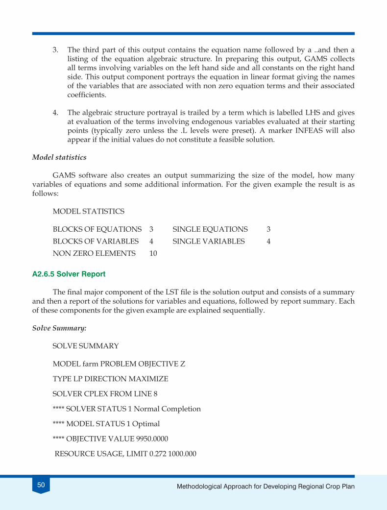
50 Methodological Approach for Developing Regional Crop Plan
3. The third part of this output contains the equation name followed by a ..and then a listing of the equation algebraic structure. In preparing this output, GAMS collects all terms involving variables on the left hand side and all constants on the right hand side. This output component portrays the equation in linear format giving the names of the variables that are associated with non zero equation terms and their associated coefficients.
4. The algebraic structure portrayal is trailed by a term which is labelled LHS and gives at evaluation of the terms involving endogenous variables evaluated at their starting points (typically zero unless the .L levels were preset). A marker INFEAS will also appear if the initial values do not constitute a feasible solution.
Model statistics
GAMS software also creates an output summarizing the size of the model, how many variables of equations and some additional information. For the given example the result is as follows:
MODEL STATISTICS
BLOCKS OF EQUATIONS 3 SINGLE EQUATIONS 3BLOCKS OF VARIABLES 4 SINGLE VARIABLES 4NON ZERO ELEMENTS 10
A2.6.5 Solver Report
The final major component of the LST file is the solution output and consists of a summary and then a report of the solutions for variables and equations, followed by report summary. Each of these components for the given example are explained sequentially.
Solve Summary:
SOLVE SUMMARY
MODEL farm PROBLEM OBJECTIVE Z
TYPE LP DIRECTION MAXIMIZE
SOLVER CPLEX FROM LINE 8
**** SOLVER STATUS 1 Normal Completion
**** MODEL STATUS 1 Optimal
**** OBJECTIVE VALUE 9950.0000
RESOURCE USAGE, LIMIT 0.272 1000.000

51Methodological Approach for Developing Regional Crop Plan
ITERATION COUNT, LIMIT 2 2000000000ILOG CPLEX Nov 1, 2009 23.3.3 WEX 13908.15043 WEI x86_64/MS WindowsCplex 12.1.0, GAMS Link 34 LP status(1): optimalOptimal solution found.Objective : 9950.000000
The solution summary contains
• the marker S O L V E S U M M A R Y;
• the model name, objective variable name (if present), optimization type (if present), and location of the solve (in the echo print);
• the solver name;
• the solve status in terms of solver termination condition;
• the objective value (if present);
• somecpu time expended reports;
• a count of solver execution errors; and
• some solver specific output.
Equation solution report
The next section of the LST file is an equation by equation listing of the solution returned to GAMS by the solver. Each individual equation case is listed. For our example the reports are as follows:
LOWER LEVEL UPPER MARGINAL—— EQU OBJ . . . 1.000 —— EQU land -INF 100.000 100.000 52.000 —— EQU labor -INF 500.000 500.000 9.500
The columns associated with each entry have the following meaning,
• Equation marker ——
• EQU - Equation identifier
• Lower bound (.lo) – RHS on =G= or =E= equations
• Level value (.l) – value of Left hand side variables. Note this is not a slack variable but inclusion of such information is discussed in the Standard Output chapter.

52 Methodological Approach for Developing Regional Crop Plan
• Upper bound (.up) – RHS on =L= or =E= equations
• Marginal (.m) – dual variable, shadow price or in MCPs only complementary variable value
Variable solution report
The next section of the LST file is a variable by variable listing of the solution returned to GAMS by the solver. Each individual variable case is listed.
LOWER LEVEL UPPER MARGINAL—— VAR Z -INF 9950.000 +INF .—— VAR Xcorn . 50.000 +INF .—— VAR Xwheat . 50.000 +INF .—— VAR Xcotton . . +INF -13.000
The columns associated with each entry have the following meaning,
• Variable marker —— • VAR - Variable identifier • Lower bound (.lo) – often zero or minus infinity • Level value (.l) – solution value. • Upper bound (.up) – often plus infinity • Margninal (.m) – reduced cost or in MCPs only slack in complementary equations
Report Summary:
Report summary of the given example is given below which is self-explanatory.
**** REPORT SUMMARY : 0 NONOPT 0 INFEASIBLE 0 UNBOUNDED
EXECUTION TIME = 0.016 SECONDS 2 Mb WEX233-233 Dec 15, 2009USER: NAIP-DSSACMO G100201:1520CP-WINNCAP DC8171
**** FILE SUMMARYInput RCPModel1Untitled_2.gmsOutput I:RCPModel1Untitled_2.lst
sts

Hkk-Ï-v-+i-–jk"Vªh; oGf"k vkfFkZdh ,oe~ uhfr vuqlaèkku laLFkkuICAR – NATIONAL INSTITUTE OF AGRICULTURAL ECONOMICS AND POLICY RESEARCH
(Indian Council of Agricultural Research)P.B. No. 11305, Dev Prakash Shastri Marg, Pusa, New Delhi-110 012, INDIA
Phone : 91-11-25847628, 25848731, Fax : 91-11-25842684 E-mail : [email protected]: // www.ncap.res.in
Na
tion
al P
rin
ters
# 0
11-4
21
38
03
0, 9
811
22
07
90