Manifestations of Berry's phase in molecules and condensed matter

J. Phys.: Condens. Matter 12 (2000) R107–R143. Printed in the UK PII: S0953-8984(00)72071-6

REVIEW ARTICLE

Manifestations of Berry’s phase in molecules and condensedmatter

Raffaele RestaINFM—Dipartimento di Fisica Teorica, Universita di Trieste, Strada Costiera 11, I-34014 Trieste,Italy

Received 28 July 1999

Abstract. Since the appearance of Berry’s seminal paper in 1984, geometric phases have beendiscovered in virtually all fields of physics. Here we address molecules and solids, and we limitour scope to the Berry’s phases of the many-electron wavefunction. Many advances have occurredin very recent years relating to the theory of such phases and their observable consequences. Afterdiscussing the basic features of Berry’s phases in a generic quantum system, we specialize toselected examples taken from molecular physics and condensed matter physics; in each of thesecases, a Berry’s phase of the electronic wavefunction leads to measurable effects.

Contents

1. Introduction2. Fundamentals

2.1. The discrete (Pancharatnam’s) geometric phase2.2. Berry’s geometric phase2.3. Connection and curvature2.4. The paradigm: the Aharonov–Bohm effect

3. Features of the geometric phase3.1. Parallel transport3.2. Computing a Berry’s phase3.3. The open-path geometric phase3.4. The single-point Berry’s phase

4. The electronic Berry’s phase4.1. Wavefunctions and density matrices4.2. Independent electrons4.3. Bloch orbitals4.4. Zak’s phase

5. Manifestations of Berry’s phase5.1. The molecular Aharonov–Bohm effect5.2. Adiabatic approximation in a magnetic field5.3. Semiclassical electron dynamics in crystals5.4. Bloch oscillations and the Wannier–Stark ladder5.5. Spin-wave dynamics in crystals

0953-8984/00/090107+37$30.00 © 2000 IOP Publishing Ltd R107

R108 R Resta

6. Macroscopic polarization6.1. The problem6.2. Polarization as a Berry’s phase6.3. A lone electron in a periodic box6.4. The position operator in extended systems6.5. A crystalline system of independent electrons6.6. King-Smith and Vanderbilt’s formula6.7. Non-crystalline systems6.8. Correlated electrons and topological phase transitions

7. Conclusions

1. Introduction

The Berry’s phase takes its name from a very influential paper byMichael Berry [1], circulatedin 1983 although published in 1984. In this review I will use the name ‘Berry’s phase’ to meana geometric phase in quantum mechanics, although analogous phases occur in other domains(e.g. in classical optics or classical mechanics [2]). Berry realized that there is a very generalphenomenon, leading to observable effects in several quite different physical cases. A fewmanifestations of what we now call a Berry’s phase were known of (and understood) before:the Aharonov–Bohm (AB) effect [3–5] dating from 1959, and the so-called molecular ABeffect [6, 7] discovered even earlier [8].

Since the first one appeared in 1983, a plethora of publications have dealt with the theoryof geometric quantum phases and its applications in various fields. A very useful book [2]containing reprints and some original articles was published in 1989. Other useful publicationsof various kinds exist: general reviews [9,10]; pedagogical and/or historical presentations fornon-specialists [11–13]; and a guide to the published literature [14]. Furthermore, the conceptof a Berry’s phase is even presented in some modern quantum mechanics textbooks [15–17].

The Berry’s phase is almost ubiquitous in present-day physics: because of this,unavoidably the Berry’s phase means somewhat different things to different people. Herewe narrow the focus to the geometric quantum phases of many-electron systems and theirobservable effects. Even after thus narrowing the focus, there remain several rather differentfields and phenomenawhere theBerry’s phase plays a relevant role; therefore further selectivityis in order. The most notable omissions here concern the quantum Hall effect [18], and thephysics of superfluids in general. In these areas, which are not covered by the present review,a large amount of work is related to geometric phases; some key references are [19] and [20].

I delivered a series of lectures on the role of Berry’s phases in electronic wavefunctionsin 1995. The present review differs from the lecture notes [21] in two main respects: it is lesspedagogical, and, more importantly, it covers several outstanding advances which occurredafter that date: in the semiclassical theory of electron dynamics in crystals [22] (sections 5.3and 5.4), in the theory of spin-wave dynamics in crystals [23, 24] (section 5.5), and the novelformulation of polarization theory [25–27] (section 6). In order to keep both the size and thescope of the present review within reasonable limits, I am going to exclude discussion of anynon-Abelian geometric phase [2, 21], or any ‘geometric distance’. The latter concept is in asense complementary to that of geometric phase [28–30]: here let me just mention that somevery recent work has shown that the localization of the electronic wavefunction in insulatingcondensed systems can be measured as a geometric quantum distance [31, 32].

The plan of this work is as follows. In section 2 I introduce the basic concept of a geometricphase, starting from a discrete approach, and I show how the geometric phase is observable,using the venerable example of the AB effect [3,4]. In section 3 I present some more advanced

Berry’s phase R109

or less known features, which are relevant to the case studies which I am going to discussin the following sections. In particular, the very unconventional ‘single-point Berry’s phase’is emphasized. In section 4 I narrow the focus to a many-electron system, and I discuss therelationship between the Berry’s phase of the wavefunction and those of the single-particleorbitals. I then specialize to a crystalline system in the thermodynamic limit, where the orbitalshave the Bloch form: the occurrence of a Berry’s phase in this area was first recognized byZak in 1989 [33]. In section 5 I discuss various observable manifestations of an electronicBerry’s phase in molecular physics and in solid-state physics: the so-called molecular ABeffect [6, 7, 34]; a surprising (and little known) feature of the adiabatic approximation inmagnetic fields [35, 36]; the semiclassical electron dynamics in crystals [22] and the relatedproblem of Wannier–Stark ladders; the theory of spin-wave dynamics in crystals [23, 24].Section 6 is entirely devoted to the modern theory of dielectric polarization. The occurrenceof a Berry’s phase in the phenomenon of polarization was discovered by King-Smith andVanderbilt in 1993 [37]: this phase plays a very important role in electronic structure theoryboth as a matter of principle [38–40] and as a computational tool [41]. Outstanding advanceshave occurred since: the work of reference [37] can nowadays be regarded as a special caseof a more general—and conceptually simpler—theory, first outlined in reference [25]. Theaccount given here of polarization theory is based on this novel viewpoint, where a single-point Berry’s phase plays a major role; the implications for correlated and/or non-crystallinecondensed systems are discussed.

2. Fundamentals

2.1. The discrete (Pancharatnam’s) geometric phase

The concept of ‘geometric phase’ made its first appearance in 1956 in a paper written by theyoung Indian physicist S Pancharatnam [42, 43], which at the time went largely unnoticed inthe Western world. This paper concerns the phases of light beams, but the ideas behind itcan be applied with basically no change to the phases of the quantum states of any physicalsystem. The essential feature of Pancharatnam’s work is that of considering discrete phasechanges, at variance with the more recent work [1, 2], where continuous phase changes areusually addressed.

The present review concerns mostly the geometric properties of the many-electronwavefunction of a condensed system. When dealing with this problem, several good reasons(which will be made clear in the rest of this work) lead us to regard the discrete approachto the geometric phase as the most fundamental one. We use therefore Pancharatnam’sdiscrete approach, translated into quantum mechanical language [44], as the starting pointfor introducing our main subject.

Let us assume that a generic quantum Hamiltonian has a parametric dependence:

H(ξ)|ψ(ξ)〉 = E(ξ)|ψ(ξ)〉 (1)

where the parameter ξ is defined in a suitable domain: a two-dimensional real ξ has beenchosen for display in figure 1. I start by discussing the most general case, and therefore for thetime being I do not specify which quantum system is described by this Hamiltonian, nor whatthe physical meaning of the parameter ξ is. To give an idea with one particular example,H(ξ)could be the electronic Hamiltonian of a molecule in the Born–Oppenheimer approximation,and ξ a suitable nuclear coordinate.

The state vectors |ψ(ξ)〉 are all supposed to reside in the same Hilbert space: this amountsto saying that the wavefunctions are supposed to obey ξ-independent boundary conditions. We

R110 R Resta

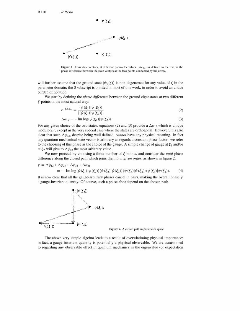
Figure 1. Four state vectors, at different parameter values. ϕ12, as defined in the text, is thephase difference between the state vectors at the two points connected by the arrow.

will further assume that the ground state |ψ0(ξ)〉 is non-degenerate for any value of ξ in theparameter domain; the 0 subscript is omitted in most of this work, in order to avoid an undueburden of notation.

We start by defining the phase difference between the ground eigenstates at two differentξ-points in the most natural way:

e−iϕ12 = 〈ψ(ξ1)|ψ(ξ2)〉|〈ψ(ξ1)|ψ(ξ2)〉|

(2)

ϕ12 = −Im log〈ψ(ξ1)|ψ(ξ2)〉. (3)

For any given choice of the two states, equations (2) and (3) provide a ϕ12 which is uniquemodulo 2π , except in the very special case where the states are orthogonal. However, it is alsoclear that such ϕ12, despite being well defined, cannot have any physical meaning. In factany quantum mechanical state vector is arbitrary as regards a constant phase factor: we referto the choosing of this phase as the choice of the gauge. A simple change of gauge at ξ1 and/orat ξ2 will give to ϕ12 the most arbitrary value.

We now proceed by choosing a finite number of ξ-points, and consider the total phasedifference along the closed path which joins them in a given order, as shown in figure 2:

γ = ϕ12 +ϕ23 +ϕ34 +ϕ41= − Im log〈ψ(ξ1)|ψ(ξ2)〉〈ψ(ξ2)|ψ(ξ3)〉〈ψ(ξ3)|ψ(ξ4)〉〈ψ(ξ4)|ψ(ξ1)〉. (4)

It is now clear that all the gauge-arbitrary phases cancel in pairs, making the overall phase γa gauge-invariant quantity. Of course, such a phase does depend on the chosen path.

Figure 2. A closed path in parameter space.

The above very simple algebra leads to a result of overwhelming physical importance:in fact, a gauge-invariant quantity is potentially a physical observable. We are accustomedto regarding any observable effect in quantum mechanics as the eigenvalue (or expectation


value) of some Hermitian operator; here we find a kind of ‘exotic’ observable, which cannotbe expressed in terms of any Hermitian operator, being instead a gauge-invariant phase of thestate vectors.

2.2. Berry’s geometric phase

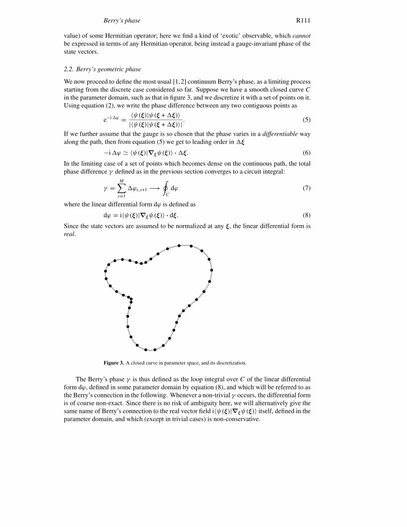
We now proceed to define the most usual [1,2] continuum Berry’s phase, as a limiting processstarting from the discrete case considered so far. Suppose we have a smooth closed curve Cin the parameter domain, such as that in figure 3, and we discretize it with a set of points on it.Using equation (2), we write the phase difference between any two contiguous points as

e−iϕ = 〈ψ(ξ)|ψ(ξ +ξ)〉|〈ψ(ξ)|ψ(ξ +ξ)〉| . (5)

If we further assume that the gauge is so chosen that the phase varies in a differentiable wayalong the path, then from equation (5) we get to leading order in ξ

−iϕ 〈ψ(ξ)|∇ξψ(ξ)〉 ·ξ. (6)

In the limiting case of a set of points which becomes dense on the continuous path, the totalphase difference γ defined as in the previous section converges to a circuit integral:

γ =M∑s=1

ϕs,s+1 −→∮C

dϕ (7)

where the linear differential form dϕ is defined as

dϕ = i〈ψ(ξ)|∇ξψ(ξ)〉 · dξ. (8)

Since the state vectors are assumed to be normalized at any ξ, the linear differential form isreal.

Figure 3. A closed curve in parameter space, and its discretization.

The Berry’s phase γ is thus defined as the loop integral over C of the linear differentialform dϕ, defined in some parameter domain by equation (8), and which will be referred to asthe Berry’s connection in the following. Whenever a non-trivial γ occurs, the differential formis of course non-exact. Since there is no risk of ambiguity here, we will alternatively give thesame name of Berry’s connection to the real vector field i〈ψ(ξ)|∇ξψ(ξ)〉 itself, defined in theparameter domain, and which (except in trivial cases) is non-conservative.

R112 R Resta

As in the discrete case outlined above, γ is a gauge-invariant quantity and therefore ispotentially observable. The main discovery of Berry’s milestone paper can in fact be spelledout as follows: there exist a whole class of observables which cannot be cast as the expectationvalues of any operator. The work which has followed Berry’s seminal paper has shown thatsuch observables occur in the most disparate physical phenomena.

In order to understand why these observables originate, we must re-examine our initialassumption of a parametric Hamiltonian, equation (1), and discuss its most fundamentalmeaning. In general, a quantum system having a parametric dependence in its Hamiltoniancannot be isolated: the parameter schematizes a kind of coupling with other variables notincluded in the Hilbert space, or more generally with ‘the rest of the Universe’, to use Berry’swords [1]. In a truly isolated system, there can be no manifestation of a Berry’s phase,and therefore observable effects may only occur in the familiar way, as eigenvalues of someHermitian operator. In this sense, the Berry’s phase is an unnecessary semiclassical concept.Its value stems from the fact that a parametric Hamiltonian allows dealing in several caseswith a part of a larger system as if it were isolated: as a trade-off, some observable effectsmay occur as gauge-invariant phases. As long as a parametric Hamiltonian is useful fordescribing the physics of a phenomenon, the corresponding Berry’s phase is also very usefuland unavoidable. This viewpoint helps in understanding why the Berry’s phase is almostubiquitous, and manifests itself in many unrelated physical problems.

2.3. Connection and curvature

We write again the main definition of the Berry’s phase for clarity:

γ =∮C

dϕ = i∮C

〈ψ(ξ)|∇ξψ(ξ)〉 · dξ. (9)

The outstanding feature of this definition is that the integrated value γ is gauge invariant andpotentially observable, while the integrand itself is largely arbitrary and lacking in any physicalmeaning.

From a purely mathematical viewpoint, the above concepts are reminiscent of a classicalcase study in electromagnetism. Wecan think of ourBerry’s connection as of an abstract ‘vectorpotential’A(ξ) in the parameter space. The vector potential has a large gauge arbitrariness, andhas no physical meaning, while its circuit integral is indeed gauge invariant and observable.Suppose for the sake of simplicity that ξ is a three-dimensional real parameter, and that ourclosed curve is contained in a simply connected domain, where the Berry’s connection isregular enough (say of class C2). Then by Stokes’s theorem

γ =∮C

A(ξ) · dξ = −∫ ∫

B(ξ) · n dσ (10)

where dσ denotes the area element in ξ-space, and the integral is performed over any surfaceenclosed by the contour C. The B-field is defined as

B(ξ) = ∇ξ × A(ξ) (11)

and in the electromagnetic analogue is obviously gauge invariant and observable.As has been emphasized, Berry’s phases occur in many different physical problems. In the

general case, there is no genuinemagnetic field, nor is ξ a space coordinate in three dimensions.Only in some special examples (as e.g. for the AB phase considered below) may it happen thatthere is a magnetic field lurking around, and that ξ is a space coordinate. However, this is byno means general. Only the mathematical structure has this close electromagnetic analogue.


To emphasize this fact, I will not use the symbols A and B in the general case. Instead, I willindicate the vector field (or Berry’s connection) as X :

X (ξ) = i〈ψ(ξ)|∇ξψ(ξ)〉. (12)

The analogue of the magnetic field in the most general case is an antisymmetric tensor field ofsecond rank (or equivalently a 2-form [45]) called the ‘curvature’. It will be indicated as Y ,and its components are

Yαβ = ∂

∂ξαXβ(ξ)− ∂

∂ξβXα(ξ) = −2 Im

⟨∂

∂ξαψ(ξ)

∣∣∣∣ ∂∂ξβ ψ(ξ)⟩. (13)

The curvature is gauge invariant; hence in principle it is physically observable at any givenξ-point.

Whenever the physics of the problem is such that the wavefunction can be taken as real,the curvature Y vanishes and the Berry’s connection is locally exact. Therefore a non-trivialBerry’s phase (i.e. γ = π ) may only occur if the ξ-domain is not simply connected.

If, instead, the nature of the problemmakes the wavefunctions unavoidably complex, thenthe curvature in general does not vanish, and one gets non-trivial Berry’s phases even withsimply connected ξ-domains. In this case the Berry’s phase γ can take any value, not just 0or π .

2.4. The paradigm: the Aharonov–Bohm effect

We illustrate the physical implications of the above mathematics for the simplest andbest known example of a geometric phase in quantum mechanics: the AB effect, whosemanifestation has been experimentally verified in several occurrences [5].

Supposewe have an electron in a box (infinite potential well) centred at the origin. We takethe ground wavefunction as real, and we write it as χ(r). The time-independent Schrodingerequation is [

p2

2m+ V (r)

]χ(r) = Eχ(r). (14)

Displacing the centre of the box to position R changes the Hamiltonian to

H(R) = p2

2m+ V (r − R). (15)

We will identify the ξ-parameter with the box position R. Because of translational invariance,the R-dependence of the state vectors is as follows:

〈r|ψ(R)〉 = χ(r − R) (16)

while the eigenvalue is R-independent.Suppose now that a magnetic field is switched on somewhere in space. Then the Hamil-

tonian becomes

H(R) = 1

2m

[p − e

cA(r)

]2

+ V (r − R) (17)

where A is the vector potential and e is the electron charge. It can be easily verified that asolution of the Schrodinger equation can be formally written in the form

〈r|ψ(R)〉 = exp

(ie

hc

∫ r

R

A(r′) · dr′)χ(r − R). (18)

But such a solution is in general not a single-valued function of r, since the phase factordepends on the path. Therefore we restrict ourselves to a less general case, where the magnetic

R114 R Resta

field is generated by a solenoid: the B-field is non-zero only within a given cylinder, andwe prevent our box from overlapping this cylinder by suitably restricting the domain of R.With such a choice, the wavefunction, equation (18), is a single-valued function of r forany fixed R, and is therefore a legitimate ground wavefunction. As for the dependence onR, equation (18) only guarantees local single valuedness, since the domain is not simplyconnected: when the system is transported on a closed path winding once round the solenoid,the electron wavefunction picks up a Berry’s phase. This phase difference can be actuallydetected in interference experiments.

The Berry’s connection of the problem is

X (R) = i〈ψ(R)|∇Rψ(R)〉 = e

hcA(R) + i

∫dr χ(r − R)∇Rχ(r − R) (19)

where the last term vanishes. Therefore the Berry’s connection is proportional—in the specificcase of the AB effect—to the ordinary vector potential. A gauge transformation in the quantummechanical sense also coincides with an electromagnetic gauge transformation, which changesA while leaving B invariant. In fact, in this example B is essentially the Berry’s curvature.The Berry’s phase is

γ = e

hc

∮C

A(R) · dR (20)

and is therefore proportional to the flux of the magnetic field across the interior of the solenoid,a space region not accessed by the quantum system.

This intriguing result was first published in 1959 [3] and was initially perceived by apart of the physicists’ community as a paradox. Instead, the AB effect is an outstanding andinescapable feature of quantum mechanics. As early as 1962–1963, R P Feynman included itin the basic physics topics he chose to teach sophomore classes [4]. Nowadays we know thatthe AB effect is just the archetype of a general class of phenomena: for these phenomena, thework of Berry gave an elegant and universal description.

The reason for the surprise engendered by the AB paper is that the quantum system residesin a region of space where there is no magnetic field B. In classical electromagnetism, the‘real’ field is B, and the vector potential A is just a mathematical construct, affected by gaugearbitrariness and non-measurable. A classical particle can only be affected by the field B atits position: no measurable effect is then possible for a charged particle which orbits outsidethe solenoid. The quantum result is qualitatively different, and somewhat counterintuitive:the system ‘feels’—through measurable effects—the presence of B in regions not accessed,or in other words it feels—in a gauge-invariant way—the ‘reality’ of the vector potential A.We may look at this effect from a very general viewpoint, already pointed out in the originalAB paper, and emphasized in Feynman’s textbook [4]. The concepts of forces and fields arecentral in classical physics, but they fade away in quantum physics. The Schrodinger equationdoes not involve forces and fields, and is necessarily expressed in terms of scalar and vectorpotentials: the ‘real’ physical quantity is A, not B. Experimental verifications of the effecthave been sought for (and found) since the early 1960s [5].

3. Features of the geometric phase

3.1. Parallel transport

In writing equation (7) we have implicitly assumed |ψ(ξ1)〉 ≡ |ψ(ξM+1)〉, i.e. a single-valuedstate vector along the continuous path. A different—and in a sense more ‘natural’—choice ispossible. Suppose for instance that the physical problem allows a real wavefunction at any ξ.


If we choose a differentiable gauge, and we require the wavefunction to be indeed real at anyξ, then this gauge is unique, and necessarily yields a vanishing connection everywhere on thepath. This implies that when closing the path the state possibly returns on itself with a signchange, i.e. the state vector is multiply valued. This state of affairs is quite general: even inthe case where the wavefunctions are complex, there is a special gauge where the phase of thestate vector is kept constant as ξ is varied by an infinitesimal amount. This gauge goes underthe name of ‘parallel transport’: it is expedient to illustrate it by means of perturbation theory.

We need to restore—for a while only—the 0 subscript for the ground state, in order to beable to deal with the excited states as well. We therefore rewrite the Berry’s connection as

X (ξ) = i〈ψ0(ξ)|∇ξψ0(ξ)〉. (21)

At first sight, the most natural tool for evaluating the gradient in equation (21) seems to beperturbation theory:

|ψ0(ξ +ξ)〉 |ψ0(ξ)〉 +∑n=0

|ψn(ξ)〉〈ψn(ξ)|H(ξ +ξ)−H(ξ)|ψ0(ξ)〉E0(ξ)− En(ξ) (22)

|∇ξψ0(ξ)〉 =∑n=0

|ψn(ξ)〉〈ψn(ξ)|∇ξH(ξ)|ψ0(ξ)〉E0(ξ)− En(ξ) . (23)

Since the excited states are orthogonal to the ground one, we get in this way a vanishing Berry’sconnection at any ξ.

The key point is that in the standard expression of perturbation theory, equation (22), aspecific choice of the gauge is implicitly made: namely, the parallel transport, which forces theinfinitesimal change in |ψ0(ξ)〉 to be orthogonal to |ψ0(ξ)〉 itself. This is a perfectly legitimatechoice, but when we go continuously round the closed path the state vector in general returnson itself only modulo a phase factor, which is indeed the Berry’s phase of the path. In otherwords parallel transport is incompatible with a state vector which is globally single valued—asa function of ξ—on the closed path.

In the previous sections, we have used a single-valued state vector throughout. This choicecan be made compatible with perturbation theory only if we rewrite equation (22) in the moregeneral form

|ψ0(ξ +ξ)〉 e−iϕ

[|ψ0(ξ)〉 +

∑n =0

|ψn(ξ)〉〈ψn(ξ)|H(ξ +ξ)−H(ξ)|ψ0(ξ)〉E0(ξ)− En(ξ)

](24)

where ϕ is an arbitrary gauge phase. Since we want it to vanish when ξ = 0, the gaugephase must be linear in ξ; we thus write equation (24) to leading order as

|ψ0(ξ +ξ)〉 (1 − iϕ)|ψ0(ξ)〉 +∑n =0

|ψn(ξ)〉〈ψn(ξ)|H(ξ +ξ)−H(ξ)|ψ0(ξ)〉E0(ξ)− En(ξ) . (25)

In this way we easily get an arbitrary phase difference—and in general a non-vanishing Berry’sconnection—since

〈ψ0(ξ)|ψ0(ξ +ξ)〉 1 − iϕ. (26)

A suitable choice of the gauge phase in equation (24) restores a single-valued behaviour of thestate vector round the path.

3.2. Computing a Berry’s phase

It has been shown in the previous section that a straightforward implementation of perturbationtheory cannot provide the Berry’s phase as a loop integral of the connection. The discrete

R116 R Resta

approach of section 2.1, instead, is the practical tool which is implemented in actual calc-ulations. Berry’s phases in condensed matter are routinely evaluated as [39]

γ =M∑s=1

ϕs,s+1 = −Im logM∏s=1

〈ψ(ξs)|ψ(ξs+1)〉 (27)

in the limit of largeM . This expression, besides its usefulness, is even important as a matterof principle.

The discrete formulation is more general than the (more traditional [2]) continuum one,since it does not assume any regularity of the phase along the path. In fact, following thepresent discrete approach, one has a well defined limiting γ even if the phase of |ψ(ξ+ξ)〉 isallowed to vary discontinuously forξ → 0. The differentiability of the local phase becomesunnecessary for defining a Berry’s phase over a continuum path.

A pathological behaviour of the local phase has some relevance for numerical work, andactually manifests itself in practical calculations. Suppose the state |ψ(ξ)〉 is obtained bynumerical diagonalization over a finite basis. Then the phase at each ξ-point is chosen—essentially at random—by the diagonalization routine, and shows no regularity at all when theset becomes denser and denser. Notwithstanding this, the phase γ defined as in equation (27)does converge to a meaningful value.

The role of perturbation theory could be rescued if, instead of writing γ as the loop integralof the connection, we write it as the surface integral of the curvature. In fact the latter quantity,being gauge invariant, can be safely expressed by means of perturbation theory within theparallel-transport gauge. Using equation (23) we recast equation (13) as

Yαβ = −2 Im∑n=0

〈ψ0(ξ)|∂H(ξ)/∂ξα|ψn(ξ)〉〈ψn(ξ)|∂H(ξ)/∂ξβ |ψ0(ξ)〉[E0(ξ)− En(ξ)]2 . (28)

This expression could be actually implemented, although its computational appeal is verylimited: it would require in fact calculating all the excited states at any ξ.

The expression of equation (28) shows that the curvature is singular at the values of ξ

where the ground state is degenerate with the first excited state. This fact has importantconsequences, particularly in those cases where the wavefunction can be taken as real. In suchcases, the Berry’s phase on a curve C can assume the value γ = π only if C encircles suchdegeneracy points. From this follows that if ξ is a d-dimensional parameter, the manifoldof the singular points of the curvature needs to be at least (d − 2)-dimensional to ensuremultiple connectiveness, and hence to produce a non-trivial Berry’s phase. In the cases wherethe wavefunction must be taken as complex, instead, singularities are no longer required toproduce a non-trivial Berry’s phase.

3.3. The open-path geometric phase

We start again from the discrete four-point introductory example of section 2.1, illustrated infigure 2, but now we consider an open path, as in figure 4. It is then obvious that the totalphase difference along the path cannot be gauge invariant in general: but we only consider thevery special case where—because of some specific symmetry of the physical problem—theHamiltonian at ξ4 is unitarily equivalent to the one at ξ1; i.e.,

H(ξ4) = W−1H(ξ1)W (29)

where W is a fixed unitary operator, given by the symmetry of the physical problem. Thenit is clear that we might like to choose the eigenstate at ξ4 as |ψ(ξ4)〉 = W−1|ψ(ξ1)〉, thusimposing a preferred phase relationship amongst the eigenstates at the initial and final points


Figure 4. An open path in parameter space

of the path. In this way we are able to define a gauge-invariant phase difference along the openpath as

γ = ϕ12 +ϕ23 +ϕ34= − Im log〈ψ(ξ1)|ψ(ξ2)〉〈ψ(ξ2)|ψ(ξ3)〉〈ψ(ξ3)|W−1|ψ(ξ1)〉. (30)

We will call such a phase the open-path geometric phase.I have used four points for pedagogical purposes. It is worth noticing that, in the closed-

path case, one needs at least three points (and three Hamiltonian diagonalizations) in order toget a non-trivial γ -value. At variance with this, in the open-path case any number of pointsprovides in principle a non-trivial γ , i.e. a γ -value different from zero (modulo 2π ).

The open-path phase is easily generalized to the continuum limit like the ordinary (closed-path) Berry’s phase:

γ = i∫C

〈ψ(ξ)|∇ξψ(ξ)〉 · dξ (31)

where now C is an open curve connecting the distinct points ξinitial and ξfinal. This phasedepends on the path C and is gauge invariant, provided the gauges are so chosen that

|ψ(ξfinal)〉 = W−1|ψ(ξinitial)〉 (32)

thus enforcing relative phase coherence between the final and initial points. This peculiar kindof geometric phase was first discussed by Zak [46].

The alternate viewpoint would be to choose the parallel-transport gauge, in which case theline integral is formally zero, but the state vector at the final point no longer fulfils equation (32).Instead, parallel transport yields

|ψ(ξfinal)〉 = eiγW−1|ψ(ξinitial)〉 (33)

where again γ is the geometric phase of the problem.

3.4. The single-point Berry’s phase

The extreme case for the open-path geometric phase is a two-point path, requiring only oneHamiltonian diagonalization:

γ = −Im log〈ψ(ξ1)|W−1|ψ(ξ1)〉. (34)

Whether even in this extreme case the phase γ still deserves the name of a geometric phase isa matter of pure semantics: indeed, the form of equation (34) is often referred to as the ‘single-point Berry’s phase’ [26]. It is convenient to perform a double change of sign in equation (34)and to express the single-point Berry’s phase as

γ = Im log〈ψ |W |ψ〉 (35)

R118 R Resta

where the parameter ξ is no longer needed.The name ‘single-point Berry’s phase’ looks almost like an oxymoron. In fact we have

stressed above that a geometric phase is an observable which cannot be cast as the expectationvalue of any operator, while instead the main ingredient of equation (35) is indeed theexpectation value of the operator W (unitary and not Hermitian): but the observable is thephase of this expectation value, and not the expectation value itself. We could thus say thatequation (35) is a Berry’s phase ‘in disguise’.

The single-point Berry’s phase manifests itself as a very important observable in modernelectronic structure theory. In fact, the macroscopic polarization of an extended system can beexpressed precisely in the form of equation (35), where ψ must be identified with the many-bodywavefunction (obeyingBorn–vonKarman boundary conditions), and the unitary operatorW with a suitable many-body operator, first introduced in reference [25], and sometimesreferred to as the ‘many-body phase operator’.

A large part of this review is about the modern theory of polarization, and we base ourpresentation very much on the concept of the single-point Berry’s phase. This very recentdevelopment is important both as a matter of principle [25–27, 32] and as a tool used inactual computations [47,48]. We will show in section 6.6 how the disguised geometric phaseof equation (35) is very naturally linked to other, more traditional, geometric phases whichoccurred in previous formulations of the polarization theory [37–39].

4. The electronic Berry’s phase

4.1. Wavefunctions and density matrices

We wrote down a Hamiltonian at the very beginning, equation (1), but then the Hamiltonianquickly disappeared from our consideration. In fact, the only role of the Hamiltonian is tosingle out the relevant state in the Hilbert space at a given ξ. We have assumed that the relevantstate is the ground state of a given Hamiltonian, but strictly speaking this is unnecessary. Inorder to define a Berry’s phase, it is enough to specify the projector over the one-dimensionalmanifold spanned by the relevant state, which coincides with the (pure-state) density matrix:

ρ(ξ) = |ψ(ξ)〉〈ψ(ξ)| (36)

as a function of ξ. In equation (36), we assume |ψ(ξ)〉 normalized, and having an arbitraryphase. Of course the density matrix is gauge invariant.

The Berry’s phase of the problem can then be cast in a transparent way as an explicitfunction of ρ(ξ). Consider the simple discrete example discussed at the beginning. Thenequation (4) can be recast as the quantum mechanical trace of a product of density matrices:

γ = −Im log tr ρ(ξ1)ρ(ξ2)ρ(ξ3)ρ(ξ4) (37)

where the gauge invariance is now transparent. Analogously, the single-point Berry’s phaseof equation (35) is cast as

γ = Im log trW ρ. (38)

In the present work we are mostly concerned with cases where the state vector |ψ(ξ)〉 isa many-electron wavefunction. Since from now on it is essential to distinguish theN -electronwavefunction from the one-particle orbitals, we will use a capital letter for the former. Thewavefunction is therefore written in Schrodinger representation as

|!(ξ)〉 → 〈x1,x2, . . . ,xN |!(ξ)〉 (39)

where xi ≡ (ri , σi) are the space and spin coordinates of the ith electron.


As discussed above, a Hamiltonian is not strictly needed. However, it is convenientto assume that |!(ξ)〉 is the ground state of a many-electron Hamiltonian H(ξ), whosedependence on the parameter ξ can be due to the one-body term, to the two-body term, orto both. We also assume that the ground state is non-degenerate at any point of the path.A relevant issue in the framework of Berry’s phases is the kind of boundary conditions weassume for the wavefunction. First of all—as observed above—the boundary conditions mustbe ξ-independent. Then we must distinguish between two rather different cases.

(i) Case one. If the electronic system is finite, such as for a molecule, we typically assumeL2

(square-integrable) wavefunctions. Supposing there is no magnetic field (and neglectingspin–orbit effects), the wavefunction can then be safely taken as real. In this case the onlyallowed value for a non-trivial Berry’s phase is π (modulo 2π ): this amounts to sayingthat the wavefunction changes sign when transported parallel round the closed path. Thisoccurrence is the so-called molecular AB effect, whose essential features are discussedbelow, in section 5.1; for a comprehensive review, refer to reference [7], and for a textbookpresentation to reference [34].

(ii) Case two. Whenever the wavefunctions must be complex, the Berry’s phase can take anyvalue. This happens in the presence of magnetic fields, such as in the cases discussed insection 2.4 above and in section 5.2 below, or as in the quantum Hall effect, not coveredby this review. But wavefunctions are unavoidably complex—even in the absence of amagnetic field—in a non-centrosymmetric system whenever we assume periodic Born–von Karman boundary conditions for the wavefunction, as is almost mandatory in dealingwith extended systems. This is precisely the case dealt with in section 6; indeed, a Berry’sphase γ measures the macroscopic polarization of a non-centrosymmetric many-electronsystem in suitable units.

The density matrix in equation (37) must be understood as the full many-body densitymatrix |!(ξ)〉〈!(ξ)|, acting on theN -particle Hilbert space. However, the physical propertieswhichwill be related to an electronicBerry’s phase are typically of the one-body kind: currents,charge transport, polarization, and so on. So, it is quite natural to ask the question of whetherthe Berry’s phase can be expressed only in terms of the reduced one-body electronic densitymatrix

ρ(1)ξ (x,x

′) = N

∫dx2 · · · dxN 〈x,x2, . . . ,xN |!(ξ)〉〈!(ξ)|x′,x2, . . . ,xN 〉 (40)

as a function of the parameter ξ. This would be a major step forward, since the N -electronwavefunction contains messy and redundant information [49]. The answer to this majorquestion is unfortunately ‘no’ in general: Berry’s phase is essentially a many-body observable.In fact, the reduced density matrix is the partial trace over N − 1 variables of the many-bodyone; but in equation (37) we are in general not allowed to take partial traces before evaluatingthe operator product. There is however a very important exception, discussed next: the caseof independent electrons. This concerns mean-field theories such as the Hartree–Fock orKohn–Sham theory. It also concerns some approximate forms of many-body Green’s functiontheory [50, 51].

4.2. Independent electrons

We study here the case where the N -electron wavefunction is uncorrelated, and has thereforethe form of a single Slater determinant:

|!(ξ)〉 = 1√N !

|ψ1(ξ)ψ2(ξ) · · ·ψN(ξ)| (41)

R120 R Resta

where ψj(ξ) are the occupied spin orbitals, taken as orthonormal. As stated above, we referto either Hartree–Fock orbitals or to Kohn–Sham orbitals.

An arbitrary unitary transformation of the occupied spin orbitals amongst themselvesprovides the same many-body wavefunction, times a constant gauge phase factor [49]. Whatdetermines the relevant state at a given ξ is only the projector over theN -dimensional manifoldof the occupied one-particle spin orbitals, which coincides with the one-body reduced densitymatrix of the uncorrelated wavefunction:

ρ(1)ξ (x,x

′) =N∑i=1

〈x|ψi(ξ)〉〈ψi(ξ)|x′〉. (42)

We will identify a gauge transformation with anN ×N unitary matrix U(ξ), which leaves thereduced density matrix invariant.

Nextwewish to express theBerry’s phase of themany-particle state, as defined in section 2,in terms of the spin orbitals. We start from equation (3):

ϕ12 = −Im log〈!(ξ1)|!(ξ2)〉 (43)

and we recognize that the overlap amongst two determinants is equal to the determinant of theoverlap matrix amongst the occupied spin orbitals:

〈!(ξ1)|!(ξ2)〉 = det S(ξ1, ξ2). (44)

Explicitly, the elements of the N ×N matrix S are

Sij (ξ1, ξ2) = 〈ψi(ξ1)|ψj(ξ2)〉. (45)

Therefore the Berry’s phase of the N -electron state over anM-point discrete closed path canbe written as

γ =M∑s=1

ϕs,s+1 = −Im logM∏s=1

det S(ξs , ξs+1). (46)

It can be straightforwardly verified that γ defined in equation (46) is gauge invariant, providedthe spin orbitals at s = 1 and s = M + 1 are the same (same phases, same N -ordering).

Taking the continuum limit of equation (46) is straightforward. The Berry’s connection is

X (ξ) = i〈!(ξ)|∇ξ!(ξ)〉 = i∇ξ′ log det S(ξ, ξ′)∣∣ξ′=ξ

. (47)

We may also exploit the well known matrix identity [52]:

det expA = exp trA (48)

which applied to A = log S yields

∇ξ′ log det S(ξ, ξ′) = tr∇ξ′ log S(ξ, ξ′) = trS−1(ξ, ξ′)∇ξ′S(ξ, ξ′). (49)

Since the overlap at ξ = ξ′ coincides with the identity, we recast the Berry’s connection as

X (ξ) = i tr∇ξ′S(ξ, ξ′)∣∣ξ′=ξ

= iN∑i=1

〈ψi(ξ)|∇ξψi(ξ)〉 (50)

and the continuum Berry’s phase as

γ =∮C

X (ξ) · dξ = iN∑i=1

∮C

〈ψi(ξ)|∇ξψi(ξ)〉 · dξ. (51)

We recognize in equation (51) precisely the sum of the Berry’s phases of each individualspin orbital. It may happen that the occupied orbitals are energy degenerate at some ξ-points,in which case there is some ambiguity in defining the ξ-dependence of each orbital separately.


This fact does not cause any problem for the Berry’s phase, which is uniquely defined once theprojector on the occupied spin orbitals is provided as a function of ξ. A sufficient conditionfor having a well defined Berry’s phase is that the highest occupied orbital is separated by afinite gap from the lowest unoccupied one at any point of the path.

Finally, it is important to point out that the separation of the many-body Berry’s phase intothe sum of single-body Berry’s phases of the orbitals is valid, in general, only in the continuumlimit. In numerical work the integral is evaluated as a finite sum, actually using equation (46),and it is essential to retain the determinantal form in order to preserve gauge invariance.

4.3. Bloch orbitals

So far, we have considered the most general many-electron system, and the most generalparameter ξ occurring in the electronic Hamiltonian. We now consider a very special case:independent electrons in a crystalline system.

The orbitals have the Bloch form:

ψnq(r + τ ) = eiq·τψnq(r) (52)

where τ is a lattice translation and q is the Bloch quasimomentum: a continuous variable inthe thermodynamic limit. The Bloch orbitals are solutions of mean-field (Hartree–Fock orKohn–Sham) Schrodinger equation:[

1

2mp2 + V (r)

]ψnq(r) = εn(q)ψnq(r) (53)

where for the sake of simplicity we assume a local potential. No major complication arises fornon-local potentials, such as are needed for state-of-the-art pseudopotential calculations, offor dealing with Fock exchange. Notice that we are thus using a q-independent Hamiltonian,equation (53), and q-dependent (quasiperiodic over the elementary cell) boundary conditions,equation (52).

The Bloch functions can be rewritten as

ψnq(r) = eiq·runq(r) (54)

where the us obey periodic boundary conditions over the elementary cell:

unq(r + τ ) = unq(r). (55)

The Schrodinger equation takes then the form[1

2m(p + hq)2 + V (r)

]unq(r) = εn(q)unq(r). (56)

All this is very trivial indeed, but I wish to point out the dual role of the boundary conditionsunder such transformation. Switching from equations (52) and (53) to equations (55) and(56) one maps the eigenvalue problem into a q-dependent Hamiltonian, with q-independentboundary conditions. This is precisely the typical case where it makes sense investigating thepossible occurrence of a geometric phase: the Hamiltonian depends on a parameter, while theeigenstates all reside in the same Hilbert space (that is, obey parameter-independent boundaryconditions). We therefore identify the parameter ξ with the Bloch vector q: notice also that qappears in the Hamiltonian, equation (56), as a kind of ‘vector potential’, although nomagneticfield is present.

According to our general formulation, the Berry’s connection of the nth band is

X (q) = i〈unq|∇qunq〉 (57)

R122 R Resta

while the corresponding curvature is

Yαβ(q) = ∂

∂qαXβ(q)− ∂

∂qβXα(q) = −2 Im

⟨∂

∂qαunq

∣∣∣∣ ∂∂qβ unq⟩. (58)

This antisymmetric Cartesian tensor can be written in vector form as

Ωα(q) = 1

2εαβγYβγ (q) = −εαβγ Im

⟨∂

∂qβunq

∣∣∣∣ ∂∂qγ unq⟩

(59)

or in more compact notation:

Ω(q) = −Im〈∇qunq| × |∇qunq〉 = i〈∇qunq| × |∇qunq〉. (60)

The curvature is gauge invariant and, therefore, corresponds in principle to a physicalobservable. In fact, Ω occurs in the semiclassical dynamics of crystalline electrons, discussedbelow in sections 5.3 and 5.4.

4.4. Zak’s phase

We are interested in the integral of the Berry’s connection for Bloch electrons, equation (57),over an open curve C connecting the points qinitial and qfinal:

γ = i∫C

〈unq|∇qunq〉 · dq. (61)

We only consider the case where the difference qfinal − qinitial is a reciprocal-lattice vectorG; at these two points, the Bloch eigenfunctions obey the same Schrodinger equation, equ-ation (53), and the same boundary conditions, equation (52). It is therefore very natural toimpose |ψnqfinal〉 ≡ |ψnqinitial〉, where the same phase is chosen: this goes under the name of‘periodic gauge’. Owing to equation (54), we have for un the relationship

unqfinal(r) = e−iG·runqinitial(r). (62)

Comparing now equations (61) and (62) to equations (31) and (32), we recognize in γ anopen-path geometric phase, where the unitary operatorW of equation (32) has to be identifiedwith the multiplicative operator eiG·r in Schrodinger representation.

If there are several occupied bands, we may consider the sum of their geometric phasesas a whole:

γ = inb∑n=1

∫C

〈unq|∇qunq〉 · dq (63)

where nb is the number of occupied bands. In the case of band crossings, there is somearbitrariness in identifying the nth band as a function of q. According to the discussion whichfollows equation (51), the total phase is gauge invariant and unaffected by such arbitrariness,provided that the nb occupied bands do not cross the empty ones at any point of the path.

The occurrence of the geometric phase γ , equation (61), in the band theory of solids wasfirst discovered by Zak [33], who identified its observable effects inWannier–Stark ladders (seebelow, section 5.4). Only much later, owing to King-Smith and Vanderbilt [37], was it realizedthat Zak’s phase has another outstanding manifestation: namely, macroscopic polarization incrystalline dielectrics. More will be said below about this (section 6).

A final comment is in order about how to compute amulti-band Zak’s phase, equation (63);more details can be found in references [21, 39]. We define the overlap matrix

Snn′(q, q′) = 〈unq|un′q′ 〉. (64)


Before discretizing the line integral, it is essential to convert the trace of S appearing inequation (63) into a determinant, using the same algebra as in section 4.2. Discretizing theopen path withM + 1 points qs we have

γ = inb∑n=1

∫C

〈unq|∇qunq〉 · dq → −Im logM−1∏s=0

det S(qs , qs+1) (65)

where, according to equation (62), we define

Snn′(qM−1, qM) = 〈unqM−1 |e−iG·r|un′q0〉. (66)

5. Manifestations of Berry’s phase

5.1. The molecular Aharonov–Bohm effect

The effect which nowadays is called the molecular AB effect [7] was first predicted asearly as 1958 [8], and historically is the first occurrence of a geometric phase in quantummechanics [6, 15]. It concerns the ionic motion in the adiabatic approximation, and isobservable through some peculiar features of the rotovibrational spectra.

The real parameter ξ coincides with a set of ionic coordinates, and is in general d-dimensional; the state vector |!(ξ)〉 is the electronic wavefunction in the Born–Oppenheimerapproximation, and Berry’s connection, equation (12), acts formally as a vector potential inthe effective Hamiltonian which governs the ionic motion. Notice that there is no genuinemagnetic field in this problem, hence the name ‘geometric vector potential’ which is oftenused. Since the wavefunction can be taken as real, the only possible value for a non-trivialBerry’s phase is π .

We start from the complete Hamiltonian H of an isolated molecular system, and weexplicitly separate the nuclear kinetic energy:

H(ξ, [x]) = 1

2

d∑α,β=1

M−1αβ pαpβ +H(ξ, [x]) (67)

where [x] indicates the electronic degrees of freedom collectively, pα = −ih ∂/∂ξα is thecanonical momentum conjugate to ξα , and the inverse mass matrix M−1 in general may be afunction of ξ, but not of the momenta.

The Born–Oppenheimer approximation starts by writing the eigenfunctions of equ-ation (67) in the Schrodinger representation as the product 〈[x]|!(ξ)〉-(ξ). Our aim isobtaining an effective Schrodinger equation for the nuclear wavefunction -(ξ), where theelectronic degrees of freedom have been integrated out. We start by considering the effect ofthe canonical nuclear momentum p on the product ansatz:

p|!(ξ)〉-(ξ) = −ih|!(ξ)〉 ∇ξ-(ξ)− ih |∇ξ!(ξ)〉-(ξ). (68)

We then multiply by the electronic eigenbra 〈!(ξ)| on the left, thus integrating over theelectronic degrees of freedom. We get the effective nuclear momentum π acting on - as

π-(ξ) = −ih[∇ξ + 〈!(ξ)|∇ξ!(ξ)〉]-(ξ). (69)

We easily recognize the ‘geometric vector potential’ anticipated above.Whenever the timescales of nuclear and electronicmotions are well separated the coupling

between different electronic states can be neglected, and the adiabatic approximation allowsus to treat the slow variable ξ inH(ξ, [x]) as a classical parameter. The electronic eigenvalue

R124 R Resta

E(ξ) of a given state (say the ground one) plays therefore the role of a (scalar) potential fornuclear motion, whose effective Hamiltonian acting on -(ξ) is then

Heff = 1

2

d∑α,β=1

M−1αβ παπβ + E(ξ). (70)

Whenever the ionic motion is purely classical, governed by Newton’s equation, the vector-potential-like term in equation (69) is irrelevant: the corresponding ‘magnetic field’ is in factidentically vanishing along the nuclear trajectory on the Born–Oppenheimer surface.

The interesting effects arise when one quantizes the nuclear degrees of freedom, usingequation (70) as the effective Hamiltonian in the Schrodinger equation for nuclear motion,whose eigenvalues provide the rotovibrational spectrum of the molecule. Notice that we haveexplicitly neglected any coupling to the higher electronic states, and thus we apparently arestrictly within the adiabatic approximation. But in fact the Berry’s connection in equation (69)accounts for effects which are absent within the ‘naive’ adiabatic approximation, and thereforeit amounts to the first step beyond it.

In most of the pre-Berry literature, the vector-potential-like term in equation (69) isneglected, or not evenmentioned: π is directly identifiedwith the canonical nuclearmomentum−ih∇ξ. The reasons are the following. In a molecular problem, one typically assumes L2

boundary conditions, i.e. vanishing wavefunctions at infinity. Then, in the absence of anexternal magnetic field and of spin–orbit interaction, the electronic wavefunctions can be takenas real at any given ξ, apparently with no loss of generality. For real electronic wavefunctions,the nuclear kinetic momentum π is identical to the canonical one p. The problem arises whenwe follow the adiabatic evolution along a closed path in ξ-space.

If we insist in requiring a real electronic wavefunction, having a continuous dependenceon ξ, then when we close the loop the electronic wavefunction may undergo a sign change.In such a case, corresponding to an electronic Berry’s phase of π , the ionic wavefunction-(ξ) must undergo a sign change as well, since the total wavefunction must be single-valued. This sign change is a boundary condition which modifies the spectrum of theeffective nuclear Hamiltonian Heff , and which has in fact remarkable observable effects onthe rotovibrational spectrum of some molecules, first predicted in 1958 [8]. A sign change inthe nuclear wavefunction corresponds in fact to half-odd-integer quantum numbers for somerotovibrational levels.

The alternate description of the same phenomenon—originally due to Mead and Truhlar[53]—requires a single-valued electronic wavefunction, which can be simply realized if weallow it to be complex. In this case the Berry’s connectionX (ξ) = i〈!(ξ)|∇ξ!(ξ)〉 no longervanishes, and we must write the kinetic momentum as

π = −ih∇ξ − hX (ξ). (71)

The effectiveHamiltonian, equation (70), nowexplicitly contains the geometric vector potentialX . The classical motion of the ions on the Born–Oppenheimer surface is unaffected by thisextra term, since the corresponding ‘magnetic field’Y , equation (13), vanishes on the classicaltrajectory of the nuclei. However, as soon as we wish to quantize the nuclear rotovibrations,the Berry’s connection shows up in producing non-trivial interference effects in the nuclearwavefunction. These may dramatically affect the spectrum, allowing for half-odd-integerquantum numbers. When the phenomenon is described in this way, one sees very clearly theanalogy with the standard AB effect. In fact, although there is no physical magnetic field B,we have a curvature Y which plays the same role. The curvature Y vanishes on the classicaltrajectory, but we get a non-trivial Berry’s phase π whenever the nuclear trajectory winds onceround a locus of δ-like singularities of Y . What determines the Berry’s phase in fact is the


flux of the curvature through a surface whose boundary is the nuclear trajectory, although thenuclear configuration never visits the singular points. As explained in section 2, the effectis possible only if the manifold of the singular points is at least (d − 2)-dimensional: suchsingular points are those where the given Born–Oppenheimer surface becomes degenerate withthe Born–Oppenheimer surface of a different electronic state. Such loci of singularities arecalled ‘conical intersections’ [6, 7].

The previous considerations show that the effective Hamiltonian for ionic motion, equ-ation (70), picks up the important topological feature of the electronic spectrum, and in partic-ular of the lowest excited state. Surprisingly, this happens despite the fact that equation (70)has been indeed derived with explicit neglect of any coupling to the higher electronic states.

The smallestmolecular systemwhere themolecularABeffect is possible is a trimer, havingthree internal coordinates (e.g. the three internuclear distances). An experiment performed in1986 indicated the presence of a Berry phase in Na3 clusters [54]: the interpretation of thesedata was later challenged [55–58]. A less controversial case appears to be Li3, for which morerecent measurements are available [59].

Finally, letmemention that aBerry’s phase of the samekind as discussed here for the boundstates of the ions manifests itself even in processes of scattering between molecular species.The phase affects the scattering amplitudes and the rates for chemical reactions. The simplestand most studied [60] example of this class of phenomena is the reaction H + H2 → H2 + H.

5.2. Adiabatic approximation in a magnetic field

We study in this section the case where a genuine magnetic field, generated by some externalsource, acts on the molecular system. The Hamiltonian of equation (67) is then modifiedby the addition of a vector potential term in the kinetic energies of both the nuclei and theelectrons. Proceeding as in the zero-field case, one writes an ansatz wavefunction and arrivesat the effective Hamiltonian for the ionic motion, equation (70), where an extra term must beadded to the kinetic momentum π of equation (71). There are thus two vector potentials in theeffective nuclear Hamiltonian: a geometric one, and a genuinely magnetic one.

However, with respect to the zero-field case, there is a qualitative difference whoseimportance is overwhelming. Since the electronic Hamiltonian is no longer invariant undertime reversal, the electronic wavefunction is necessarily complex. In this case no degeneracybetween different Born–Oppenheimer surfaces is needed in order to produce a non-trivialBerry’s phase: on the contrary, the Berry’s phase will be in general non-zero along any path inξ-space. Furthermore, the Berry’s curvatureY , equation (13), will be in general non-vanishingeverywhere, at variance with the zero-field case where it has only δ-like singularities (on theloci of degeneracy, also known as conical intersections).

Suppose we are interested in the ionic motion at the purely classical level. TheHamiltonian of equation (70)—whose kinetic momentum π includes now the two differentvector potentials—yields the Hamilton equations of motion, which can be transformed intothe Newton equations of motion; within the latter, the effects of the vector potentials appearin terms of fields, in the form of Lorentz forces. The curl of the magnetic vector potentialobviously yields the magnetic field due to the external source; the curl of the geometric vectorpotential (Berry’s curvature) yields an additional ‘magnetic-like’ field which is non-zero evenon the classical trajectory of the ions. Notice that this is at variance with the zero-field case,where the Berry’s phase had no effect on the ionic motion at the classical level, and could onlybe detected when quantizing the ionic degrees of freedom.

Within a naiveBorn–Oppenheimer approximation—whereBerry’s phases are neglected—the magnetic field acts on the nuclei as if they were ‘naked’ charges: a proper treatment must

R126 R Resta

instead account for electronic screening. This state of affairs was first recognized in 1988 bySchmelcher et al [35], who arrived at a ‘screened Born–Oppenheimer approximation’. Onlymore recently was this effect recognized as a manifestation of the Berry’s phase, in the workof Mead and co-workers [7,36]. Surprisingly, there are very few calculations of the effect: it ispretty clear, however, that the geometric term is no small correction. This is easily illustratedwith the simple case of a neutral atom moving at constant speed in a uniform magnetic field.Obviously, a neutral object is not deflected by a Lorentz force, while if we analyse themotion ofthe ion within a naive Born–Oppenheimer approximation we find that it is deflected accordingto its naked nuclear charge. The geometric vector potential solves the paradox: remarkably, the‘magnetic-like’ field due to the Berry’s phase is—in this simple example—exactly oppositeto the external magnetic field, thus providing the complete screening which is physicallyexpected.

It is worth showing how this works in detail for the hydrogen atom. In the completeHamiltonian of equation (67) we identify ξ → R and [x] → r:

H(R, r) = 1

2M

[p +

e

cA(R)

]2

+H(R, r) (72)

H(R, r) = 1

2m

[−ih∇r − e

cA(r)

]2

− e2

|r − R| . (73)

Notice that e is negative here. We then consider the electronic Hamiltonian, equation (73), asa function of the parameter R, in the symmetric gauge where A(r) = 1

2B × r. If ψ0(r) is theexact ground eigenfunction when the proton sits at R = 0, the eigenfunction at a generic R is

ψR(r) = exp

(ie

2hcr · B × R

)ψ0(r − R). (74)

The Berry’s connection X is clearly

X (R) = i〈ψR|∇RψR〉 = e

2hc〈ψR|B × r|ψR〉 = e

2hcB × R = e

hcA(R) (75)

since the R-derivative of ψ0(r − R) does not contribute. The geometric vector potential Xadds up to the kinetic momentum π which appears in the effective equation of motion for theproton. Clearly this term, equation (75), multiplied by −h as in equation (71), exactly cancelsthe magnetic vector potential acting on the naked proton, which appears in equation (72), thusproviding the complete screening discussed above.

5.3. Semiclassical electron dynamics in crystals

The semiclassical approach has proven very useful for describing the electronic dynamics inslowly perturbed crystals: it has played, over several decades, a fundamental role in the physicsof metals and semiconductors [61, 62], and in technology as well. Within the semiclassicalapproach, the dynamics of an electron in a given band is described by a wave packet centredat r, and whose crystal momentum is q: both r and q evolve slowly in time. In the absence ofcollisions, the equations of motion are usually written as

r = 1

h

∂εn(q)

∂q

hq = e

(E +

1

cr × B

) (76)

where εn(q) is the band structure of the relevant band, and E and B are the perturbing fields.


As emphasized in reference [62], the derivation of equation (76), despite the formalsimplicity of the result, is ‘a formidable task’. The early derivations date from the 1930s [63];the problem was reconsidered several times in the literature, by Slater [64], Luttinger [65],and Zak [66] among others. The most thorough analysis, due to Sundaram and Niu [22],is very recent: the main finding is that some important Berry’s phase terms are missing inequation (76). With hindsight, and having in mind other adiabatic phenomena, this finding isperhaps not too surprising.

According to Sundaram andNiu, threemajormodifications are needed in the semiclassicalequations of motion, equation (76). First: the unperturbed crystal momentum q has to bereplaced with the gauge-invariant crystal momentum hk = hq − (e/c)A(r, t); this is indeedthe analogue of the kinetic momentum π usually appearing in Hamiltonians, such as in thesimple case of equation (73). Second: the band-structure energy εn(q) needs a correction termwhich accounts for the orbital magnetization of the wave packet. Third: a Berry’s curvatureappears explicitly in the equation of motion. In this review, we focus on this last point only, andwe refer the reader to the original paper [22] for the most general case. We therefore consideronly the special case where the magnetic field vanishes, in which case the Sundaram–Niuequations of motion are

r = 1

h

∂εn(q)

∂q− q × Ω(q)

hq = eE.(77)

The extra contribution with respect to equation (76) comes from the vector field Ω(q), havingthe dimensions of a squared length: this is precisely the standard Berry’s curvature of Blochelectrons, equation (60), for the relevant band.

5.4. Bloch oscillations and the Wannier–Stark ladder

In the presence of a constant field the semiclassical equations of motion, equation (77), areeasily integrated: q(t) = eEt/h + constant, and r is then an explicit function of time. Thesemiclassical approach is, by construction, a single-band approximation: since both εn(q) andΩ(q) are periodic functions of q, one has that r is a periodic function of time. Furthermore, r isan odd function of q: therefore even the motion of r is periodic in time. Themotion of q can bethought of as periodic as well, once a reduced-zone scheme is adopted. This periodic motionof the slow variables r and q in a constant field goes under the name of ‘Bloch oscillations’.We will indicate the trajectory of this motion as r(q): this trajectory is a closed orbit in thetorus geometry of the reciprocal cell.

Next, we are going to quantize the motion of the slow variables: we will content ourselveswith a semiclassical Bohr–Sommerfeld quantization. The appropriate multidimensionalformula, known as Einstein–Brillouin–Keller quantization, is∮

C

(∂L

∂ q· dq +

∂L

∂ r· dr

)= 2πh

(m +

α

4

)(78)

whereL is the Lagrangian, C is the closed orbit r(q) at a given energyWm, and α is an integer,known as the Maslov index [67].

It is easy to prove that the semiclassical equations ofmotion, equation (77), can be obtainedfrom the Lagrangian [22]:

L = L(q, q, r, r) = −εn(q) + eE · r + hr · q + ih〈unq|∇qunq〉 · q. (79)

The only non-trivial term occurring in this proof isd

dt

∂L

∂ q= ih

d

dt〈unq|∇qunq〉 = hΩ(q)× q. (80)

R128 R Resta

Replacing the canonical momenta conjugate to q and r into equation (78) we get∮C

(ih〈unq|∇qunq〉 · dq + hq · dr) = 2πh

(m +

α

4

)∮C

(i〈unq|∇qunq〉 − r) · dq = 2π

(m +

α

4

).

(81)

This expression takes a particularly simple form in one dimension, since the trajectory in the(q, x) variables is uniquely determined by the conservation of energy:

εn(q)− eEx = constant = Wm. (82)

We thus get the discrete spectrum from equation (81):

Wm = εn + eEa

(m +

α

4− γ

2π

)(83)

where a is the lattice constant, εn is the band-energy average, and γ is Zak’s geometric phase:

εn = a

2π

∫ π/a

−π/aεn(q) dq γ = i

∫ π/a

−π/a〈un(q)|(d/dq)un(q)〉 dq. (84)

The integer m can take any value from −∞ to ∞: this spectrum is the famous Wannier–Stark ladder, first predicted by Wannier in 1960 [68, 69] without the geometric-phase term.The γ -correction was found in 1968 by Zak [70], who much later (1989) recognized it as amanifestation of the geometric phase [33]. The derivation given here follows Sundaram andNiu [22].

The presence of the γ -term in the spectrum, equation (83), is essential as a matter ofprinciple: without it, the spectrum would be disturbingly unphysical. Suppose we change thepotential by an arbitrary constant: this can be written asEx → E(x−x0), corresponding thusto a shift of origin. Clearly the spectrum must be translationally invariant: the position of thediscrete levels (with respect to the band energy) must be independent of the choice of the originx0 in the crystal cell. The geometric-phase term in equation (83) removes this drawback. Infact, the Zak’s phase does depend of the choice of the origin in the cell: the changes in the twoterms compensate†, thus ensuring the translational invariance of the spectrum.

Formany years,Wannier–Stark ladders have remained a purely academic subject. In orderto observe the phenomenon, one needs collisionless coherent motion of the carriers throughoutan entire band. Furthermore, the existence of the phenomenon, even in principle, wascontroversial [70]: the whole theory seems in fact to rely on the semiclassical approximationand on the neglect of interband coupling. The effect was first detected in 1988 by means ofoptical techniques [71]. The breakthrough was made possible by the use of a very special‘crystalline solid’: a semiconductor superlattice, whose lattice constant a is of the order of100 Å. A moderate field is then sufficient for driving the carriers all the way to the top ofthe ‘miniband’. The existence of Wannier–Stark ladders was later confirmed by a variety oftechniques [72], and for different physical systems [73].

5.5. Spin-wave dynamics in crystals

We discuss here the case of a spin wave in a crystal, which evolves in time (slowly comparedto the electronic timescales). The phenomenon has been almost invariably studied in terms ofa Heisenberg model Hamiltonian [74,75], where the continuum nature of the spin distributionis disregarded, and magnetization is schematized as localized at lattice sites. Very recently,

† The algebra to prove this is very similar to that used in reference [39] around equation (22).


Niu and Kleinman [23] have given a general formulation, which applies to real crystals andwhere the continuum nature of the spin distribution is fully accounted for. Their major resultis that a Berry curvature plays a key role in the theory. First-principles calculations based onthis theory have been performed by Gebauer and Baroni: their results for iron are in excellentagreement with experiment [76].

Quite generally, wave propagation in extended systems occurs whenever the staticequilibrium configuration is perturbed by a disturbance. The disturbance has an energy costwhich provides a restoring force. In order to establish the dynamics of the wave, one hasto identify the inertia of the system in responding to this force. This is pretty clear for theparadigmatic example of elasticwaves, where the restoring force ismeasured by the appropriateelastic modulus, and the inertia is measured by the mass density. For a spin wave withinthe standard textbook treatment [75], the Heisenberg Hamiltonian immediately provides theequilibrium configuration (ferromagnetic or antiferromagnetic, in the simplest cases), and alsoprovides the energy cost of any disturbance. The restoring force in this case is actually arestoring torque; what about the inertia? We observe first of all that the equation of motionis first order in time, and not second order as in the most usual wave equations: the torqueequals the rate of change of the (localized) spin angular momentum. If we replace the latterwith a classical angular momentum, we see that it is clearly partitioned into an inertia factor(the moment of inertia) times a kinematic factor (the angular velocity). But for a spin angularmomentum such partition is meaningless: inertia and kinematics are entangled. The modulusis fixed and only the orientation may change: the rate of change is therefore off-diagonal inthe spin components. Within the equation of motion [75], the factor which multiplies thetime derivative of the local spin—and which represents the ‘inertia’—is simply h times apure-number matrix. We could regard this as a very simple ‘geometric’ quantity.

We now switch from the idealized Heisenberg model to a real crystal, where themagnetization M(r) is a continuum vector field. For a magnetic system the equilibriummagnetization M0(r) is obviously non-zero, and can be computed using a variety of first-principles approaches. Wewish to define the energy cost of amagnetization fluctuation δ M(r),where we explicitly make the adiabatic hypothesis: the electronic wavefunction is assumed tofollow the instantaneous spin-wave configuration. Owing to this, and exploiting the variationaltheorem, one defines the total energy of the system for an arbitrary magnetization E[ M] bymeans of a constrained-minimum problem:

E[ M] = min〈!|H |!〉 (85)

where the search is performed over all the wavefunctions ! yielding the given magnetizationM(r). The unconstrained minimum of equation (85) coincides with the absolute minimumof the functional, which occurs at M0(r); for an arbitrary M(r), equation (85) defines E[ M]and ![ M].

The Cartesian components of the harmonic restoring force are therefore

Kαβ(r, r′) = δ2E[ M]

δMα(r) δMβ(r′). (86)

We then need the inertia term: as anticipated above, the outstanding finding of Niu andKleinman [23] is that the ‘inertia’ of a spin wave within the equation of motion is measuredby the appropriate Berry’s curvature of the electronic wavefunction (times h). In the notationof Gebauer and Baroni [76] this curvature is

4αβ(r, r′) = −2 Im

⟨δ![ M]

δMα(r)

∣∣∣∣∣ δ![ M]

δMβ(r′)

⟩(87)

R130 R Resta

and the equation of motion for the spin wave is

h

∫dr′ 4αβ(r, r′)Mβ(r

′) =∫

dr′ Kαβ(r, r′)Mβ(r′). (88)

In practical calculations, the magnetization fluctuation δ M(r) must be expressed in terms ofdiscrete parameters: the functional derivatives become then partial derivatives, equation (87)becomes a very standard Berry’s curvature, and the equation of motion becomes a matrixequation.

In the limiting case of the Heisenberg model the magnetization fluctuation is discretizedas a simple lattice variable; the equations of motion, equation (88), take then the usual textbookform [75]. In this limit, theBerry curvature4αβ(r, r′)becomes apure-numbermatrix, diagonalover the sites and off-diagonal in the Cartesian coordinates [24].

6. Macroscopic polarization of dielectrics

6.1. The problem

The dipole moment of any finite N -electron system in its ground state is a simple and welldefined quantity. Given the many-body wavefunction! and the corresponding single-particledensity n(r) the electronic contribution to the x-component of the dipole is

e〈X〉 = e

∫dr xn(r) = e〈!|X|!〉 (89)

where

X =N∑i=1

xi.

This looks very trivial, but we are exploiting here an essential fact: the ground wavefunctionof any finite N -electron system is square integrable and vanishes exponentially at infinity; thedensity vanishes exponentially as well.

Considering now a macroscopic solid, the related quantity is macroscopic polarization,which is very much an essential concept in any phenomenological description of dielectricmedia [77]: this quantity is ideally defined as the dipole of a macroscopic sample, divided byits volume. The point is that, when using equation (89), the integral is dominated by whathappens at the surface of the sample: knowledge of the electronic distribution in the bulkregion is not enough to unambiguously determine the dipole. This looks like a paradox, sincein the thermodynamic limit macroscopic polarization must be an intensive quantity, insensitiveto surface effects.

Macroscopic polarization in the bulk region of the solid must be determined by what‘happens’ in the bulk as well. This is the case if one assumes a model of discrete and wellseparated dipoles, a la Clausius and Mossotti: but real dielectrics are very much differentfrom such an extreme model. The valence electronic distribution is continuous, and oftenvery delocalized (particularly in covalent dielectrics). Most textbooks attempt to explain thepolarization of a periodic crystal via the dipole moment of a unit cell, or something of thekind [61, 74]. These definitions are incorrect [78]: according to the modern viewpoint, bulkmacroscopic polarization is a physical observable completely independent of the periodiccharge distribution of the polarized crystalline dielectric.

The basic clue to the solution of the polarization problem comes from some experimentalfacts. The absolute polarization of a crystal in a given state has never been measured asa bulk property, independent of sample termination. Instead, well known bulk properties


are derivatives of the polarization with respect to suitable perturbations: permittivity, pyro-electricity, piezoelectricity, effective charges (for lattice dynamics). In one important case—namely, ferroelectricity—the relevant bulk property is inferred from the measurement of afinite difference (polarization reversal). In all cases, the derivative or the difference in thepolarization is typically accessed via the measurement of a macroscopic current.

We illustrate the main concepts on the case of the piezoelectric effect: two possiblerealizations of it are shown schematically in figure 5. In (a) the crystal is uniaxially strained(along a piezoelectric axis) while kept in a shorted capacitor; in (b) the sample is strainedwhile kept isolated. Focusing on (a), we notice that the phenomenon manifests itself as a bulkcurrent traversing the sample, while nothing peculiar happens at the surfaces. Indeed the currentflowing across the shorting wire is the quantity which is actually measured in experiments.The modern theory of polarization focuses on currents as well: since it is the phase of thewavefunction which carries information about the current, it should not be too surprising thata gauge-invariant phase occurs in the theoretical description of electronic polarization.

(a) (b)

+ + + + + +

− − − − − −

Figure 5. Two possible realizations of the piezoelectric effect: (a) the sample is in a shortedcapacitor, and the current is measured; (b) the sample is isolated.

Figure 5(a) is also helpful for the purpose of understanding the root of the Berry’s phase inthe phenomenon: the quantum system is in interaction with an external apparatus, and ‘slaved’to it. We are allowed to study the quantum system as if it were isolated, but then—as emph-asized in Berry’s original paper [1]—the interaction with the ‘rest of the Universe’ gives rise toa non-trivial phase which is observable: indeed, this Berry’s phase measures the piezoelectricpolarization in suitable units. This state of affairs has to be contrasted with figure 5(b), wherethe quantum system is isolated and no Berry’s phase may occur: the polarization can beevaluated from the modulus of the wavefunction, as in equation (89). The obvious drawbackis that the whole effect appears like a surface phenomenon, while piezoelectric polarizationmust instead be an intensive bulk quantity.

6.2. Polarization as a Berry’s phase

In condensed matter physics the standard way of getting rid of undesired surface effects isto adopt periodic Born–von Karman (BvK) boundary conditions: this makes equation (89)useless, since the integrals are ill defined due to the unbounded nature of the quantummechanical position operator. Because of this fact, macroscopic polarization remained a majorchallenge in electronic structure theory for many years [78]. The breakthrough came in 1992,when the problem was approached essentially from the viewpoint of figure 5(a): a definitionbased on the wavefunctions, and not on the charge, was provided [79]. This definition hasan unambiguous thermodynamic limit, such that BvK boundary conditions and Bloch statescan be used safely. In the following months a modern theory of macroscopic polarization incrystalline dielectrics was completely established [38, 39], thanks to a major advance due toR D King-Smith and D Vanderbilt [37], who expressed polarization as a Berry’s phase. A

R132 R Resta

comprehensive account of the modern theory exists [39]. Other less technical presentationsare available as well [80–82]; for a very simplified non-technical outline see reference [40].First-principles calculations based on this theory have been performed for several crystallinematerials [41].

All of the above-quoted work refers to a crystalline systemwithin an independent-electronformulation: the single-particle orbitals have then the Bloch form, and the Berry’s phase whichprovides the polarization value is just the standard Zak’s phase of the orbitals, discussed insection 4.4. The related, but substantially different, problem of macroscopic polarization in acorrelated many-electron system was first solved by Ortız and Martin in 1994 [83]. However,according to them, polarization is defined—and computed [84, 85]—by means of a peculiar‘ensemble average’, integrating over a set of different electronic ground states; this was muchlater (1998) shown to be unnecessary. In reference [25], in fact, a simpler viewpoint is taken:the polarization of a correlated solid is expressed as a single-point Berry’s phase, of the samekind as in equation (35). This is indeed a ‘pure-state’ property, although of a rather exotickind. By the same token, it was also possible to define [21,25,26]—and to compute [47,48]—macroscopic polarization in non-crystalline systems. The presentation given here is based onthis very recent advance.

The single-point Berry’s phase provides an expression for the expectation value 〈X〉,derived in the following: equations (98) and (99). This expression must be used in the place ofequation (89) when BvK boundary conditions are adopted. The value of our definition residesin the fact that, whenever the electronic Hamiltonian is adiabatically varied, the time derivativeof 〈X〉 coincides with the macroscopic electronic current 〈Jx〉 traversing the sample. Having inmind the simple example of figure 5(a), this is precisely what is needed to define macroscopicpolarization.

All of the different versions of the theory, including the one presented here, concernphenomena where the macroscopic polarization is induced by a source other than an electricfield. Even in this case, the polarizationmay (ormay not) be accompanied by a field, dependingon the boundary conditions chosen for the macroscopic sample. The modern theory, basedon a Berry’s phase, addresses polarization differences in zero field: this concerns thereforelattice dynamics, piezoelectricity—as in the ideal experiment sketched in figure 5(a)—andferroelectricity. Notably, we do not address the problem of evaluating the dielectric constant:this can be done using alternative approaches, not based on a Berry’s phase, such as the wellestablished linear response theory [81, 86], or other more innovative theories [87].

6.3. A lone electron in a periodic box

We start by considering the simple case of a single electron within BvK boundary conditionsin one dimension: ψ(x + L) = ψ(x), where L is the imposed periodicity, typically chosento be large with respect to atomic dimensions. The electron distribution may look like theone of figure 6: intuitively, the distribution appears to have a ‘centre’ x0, which however isdefined only modulo the replica periodicity, and furthermore cannot be evaluated simply as inequation (89), i.e.

〈x〉 =∫

dx x|ψ(x)|2

precisely because of the BvK boundary conditions. Selloni et al [88] solved the problem someyears ago by means of a very elegant and far-reaching formula, presented in the following.The work of reference [25] can be regarded as the many-body generalization of it.

According to references [25,32,88], the key quantity for dealing with the position operator


0 Lx0

Figure 6. The distribution |ψ(x)|2 of a single-particle orbital within periodic Born–von Karmanboundary conditions.

within BvK boundary conditions is the dimensionless complex number z, defined as

z = 〈ψ |ei(2π/L)x |ψ〉 =∫ L

0dx ei(2π/L)x |ψ(x)|2 (90)

whose modulus is no larger than 1. The most general electron density, such as the one depictedin figure 1, can always be written as a superposition of a function nloc(x), normalized over(−∞,∞), and of its periodic replicas:

|ψ(x)|2 =∞∑

m=−∞nloc(x − x0 −mL). (91)

Both x0 and nloc(x) have a large arbitrariness: we restrict it a little bit by imposing the conditionthat x0 is the centre of the distribution, in the sense that∫ ∞

−∞dx xnloc(x) = 0.

Using equation (91), z can be expressed in terms of the Fourier transform of nloc as

z = ei(2π/L)x0 nloc

(−2π

L

). (92)

If the electron is localized in a region of space much smaller than L, its Fourier transform issmooth over reciprocal distances of the order of L−1 and can be expanded as

nloc

(−2π

L

)= 1 − 1

2

(2π

L

)2 ∫ ∞

−∞dx x2nloc(x) + O(L−3). (93)

A very natural definition of the centre of a localized periodic distribution |ψ(x)|2 is thereforeprovided by the phase of z as

〈x〉 = L

2πIm log z (94)

which is in fact the formula first proposed by Selloni et al [88]. The expectation value 〈x〉 isdefined modulo L, as expected since |ψ(x)|2 is BvK periodic. Comparing with equation (35),we notice that 〈x〉 has precisely the form of a single-point Berry’s phase: the angle is convertedinto a length by the factorL/2π , and the unitary operatorW of equation (35) has to be identifiedwith the multiplicative operator ei(2π/L)x in Schrodinger representation.

The above expressions imply 〈x〉 x0 modL; in the special case where nloc(x) can betaken as an even (centrosymmetric) function, its Fourier transform is real and equation (92)

R134 R Resta

yields indeed 〈x〉 ≡ x0 modL. In the case of extreme delocalization we have instead|ψ(x)|2 = 1/L and z = 0: hence the centre of the distribution 〈x〉, according to equation (94),is ill defined. For a more general delocalized state, we expect z to go to zero at large L [32].

We have therefore arrived at a definition of 〈x〉 within BvK boundary conditions whichhas many of the desirable features we were looking for; nonetheless, there is a property thatis even more important, and which we are going to discuss next. Suppose the potential whichthe electron moves in has a slow time dependence—as was the case in reference [88]—andwe wish to follow the adiabatic evolution of the electronic state |ψ〉. If we write |ϕj 〉 for theinstantaneous eigenstates at time t , the lowest-order adiabatic evolution of the ground-statedensity matrix is [89]

|ψ〉〈ψ | |ϕ0〉〈ϕ0| + i∑j =0

(|ϕj 〉〈ϕj |ϕ0〉

εj − ε0 〈ϕ0| − h.c.

)(95)

where the phases have been chosen in order to make |ϕ0〉 orthogonal to its time derivative |ϕ0〉.The macroscopic electrical current flowing through the system at time t is therefore

〈j〉 = e

L〈ψ |p|ψ〉 ie

L

∑j =0

〈ϕ0|p|ϕj 〉〈ϕj |ϕ0〉εj − ε0 + c.c. (96)

It is then rather straightforward to prove that 〈j〉 to lowest order in 1/L equals (e/L) d〈x〉/dt ,where 〈x〉 is evaluated using in equation (94) the instantaneous ground eigenstate:

〈j〉 e

2πIm

d

dtlog〈ϕ0|ei(2π/L)x |ϕ0〉. (97)

This finding proves the value of equations (90) and (94) in studying electron transport [88]:for similar reasons, the many-body generalization of equations (90) and (94) defines themacroscopic polarization of an extended system.

6.4. The position operator in extended systems

We are now going to consider a system ofN electrons in a cubic periodic box of side L, whereeventually the thermodynamic limit is taken: L → ∞, N → ∞, and N/L3 = n0 is constant.We also assume the ground state non-degenerate, and we deal with insulating systems only:this means that the gap between the ground eigenvalue and the excited ones remains finitefor L → ∞. BvK boundary conditions impose periodicity (of period L) in each Cartesiancoordinate and in each electronic variable separately.

We start by defining the many-body analogue of equation (90), namely, the multiplicativeoperator X = ∑N

i=1 xi , and the complex number

zN = 〈!|ei(2π/L)X|!〉. (98)

It is obvious that the operator X is ill defined in the BvK Hilbert space, while its complexexponential appearing in equation (98) is well defined; we will call this exponential the ‘many-body phase operator’ in the following. Themain result of reference [25] is that the ground-stateexpectation value of the position operator is given by the analogue of equation (94), namely

〈X〉 = L

2πIm log zN (99)

which is a quantity defined modulo L as above. As in the much simpler case of equation (89),〈X〉 is extensive. We stress that nowhere have we assumed crystalline periodicity. Thereforeour definition of 〈X〉 is very general: it applies to any condensed system, either ordered ordisordered, either independent electron or correlated.


The right-hand side of equation (99) is not simply the expectation value of an operator: itis in fact the phase of it. Indeed, our definition of 〈X〉 is a single-point Berry’s phase, convertedinto length units by the factor L/2π , and where the unitary operatorW of equation (35) has tobe identified with the many-body phase operator ei(2π/L)X. It is important to realize that thisoperator is a genuine many-body one. In general, one defines an operator to be a one-body onewhenever it is the sum ofN identical operators, acting on each electronic coordinate separately:for instance, the X-operator is one such. In order to express the expectation value of a one-body operator the full many-body wavefunction is not needed: knowledge of the one-bodyreduced density matrix is enough; I stress that, instead, the expectation value of ei(2π/L)X overa correlated wavefunction cannot be expressed in terms of the one-body density matrix.

As in the one-body case, whenever the many-body Hamiltonian is slowly varying in time,the (macroscopically averaged) electrical current density flowing through the system is givenby

〈Jx〉 = e

L3

d

dt〈X〉 = e

2πL2

d

dtIm log zN (100)

where zN is evaluated using in equation (98) the instantaneous ground eigenstate of the Hamil-tonian at time t ; this result is proved in reference [25]. Since 〈X〉 is an extensive quantity,the current density 〈Jx〉, equation (100), goes to a well defined thermodynamic limit. Noticethat the L → ∞ limit in equation (100) is a rather unconventional one, since the many-bodyphase operator in zN goes formally to the identity, but the size of the system and the numberof electrons in the wavefunction ! increase with L.

6.5. A crystalline system of independent electrons

We now specialize the above very general formulation to a simple cubic crystal of latticeconstant a, where the BvK periodicity is L = Ma. The most general crystal structure canbe dealt with by means of a simple coordinate transformation, such as the one considered inreference [39]. In the non-interacting case the single-particle orbitals can be chosen in theBloch form: there are M3 allowed Bloch vectors qs , which lie on a regular mesh in the unitreciprocal cell, where s ≡ (s1, s2, s3) and

qs = 2π

Ma(s1, s2, s3) sα = 0, 1, . . . ,M − 1. (101)

We adopt a plane-wave-like normalization for the Bloch orbitals:

〈ψnqs |ψn′qs′ 〉 = 1

a3

∫dr ψ∗

nqs(r)ψn′qs′ (r) = δnn′δss ′ (102)

where the integral is performed over the unit cell. If our insulating system has nb doublyoccupied bands, there are N = 2nbM3 independent spin orbitals: the ground wavefunctionis a Slater determinant of size N . This large determinant can be cast as the antisymmetrizedproduct ofM3 small determinants of size 2nb; each; i.e.,

|!〉 = A∏s

1

L3nb

1√(2nb)!

|ψ1qsψ1qsψ2qsψ2qs · · ·ψnbqsψnbqs | (103)

where A is the antisymmetrizer operator, and theN -body wavefunction is normalized to 1 overthe hypercube of side L.

For this wavefunction, the expectation value of the many-body phase operator, equ-ation (98), is conveniently written as

zN = 〈!|!〉 (104)

R136 R Resta

where ! is the Slater determinant of a different set of Bloch spin orbitals:

ψnqs (r) = ei(2π/Ma)xψnqs (r) (105)

and analogously for the bar (spin-down) ones. According to a well known theorem, the overlapbetween two single-determinant wavefunctions is equal to the determinant of theN ×N over-lapmatrix built out of the occupied spin orbitals. We start by noticing that the overlaps betweendifferent-spin spin orbitals vanish, while those between equal-spin ones are identical in pairs.We can therefore write

zN = (detS)2 (106)

where S is the overlap matrix for spatial orbitals, having size N/2 = nbM3, and whose

elements are

Snqs ,n′qs′ = 1

a3

∫dr ψ∗

nqs(r)ψn′qs′ (r)

= 1

a3

∫dr u∗

nqs(r)un′qs′ (r) exp

(i

[2π

Max + qs ′ · r − qs · r

])(107)

where the us are the periodic factors in the Bloch orbitals.The matrix S is very sparse: in fact, given the geometry of the qs on the regular reciprocal

mesh, the overlap integrals in equation (107) are non-vanishing only if s1 = s ′1 + 1, s2 = s ′2,and s3 = s ′3. We express the non-vanishing elements in terms of a small overlap matrix S, ofsize nb × nb:

Snn′(q, q′) = 〈unq|un′q′ 〉 = 1

a3

∫dr u∗

nq(r)un′q′(r). (108)

This same matrix has been introduced previously, in equation (64). Owing to the sparse-ness of S, its determinant factors into products of determinants of small matrices S as follows:

z1/2N = detS =

∏s1,s2,s3

det S(qs1+1,s2,s3 , qs1,s2,s3) (109)

log zN = 2M−1∑s2,s3=0

logM−1∏s1=0

det S(qs1+1,s2,s3 , qs1,s2,s3). (110)

We have

〈X〉 = 2Ma

2π

M−1∑s2,s3=0

Im logM−1∏s1=0

det S(qs1+1,s2,s3 , qs1,s2,s3) (111)

where the thermodynamic limitM → ∞ (and N → ∞) is understood. Notice, however, thatnumerical implementations exactly correspond to taking a finiteM in equation (111).

6.6. King-Smith and Vanderbilt’s formula

We have stressed in section 6.1 that, when measuring polarization, the quantity actuallymeasured is the current which traverses the sample while a given perturbation is adiabaticallyswitched on. The electronic contribution to this current is, after equation (100):

Px =∫ t

0dt 〈Jx(t)〉 = e

2πL2[Im log zN(t)− Im log zN(0)]. (112)

Notice that in the adiabatic limit t goes to infinity and J (t) goes to zero, while Px onlydepends on the initial and final states. In the special case of a crystalline system of independent


electrons we may replace equation (111) in equation (112). We exchange the arguments in S,which brings up a minus sign. We get

Px = e〈X〉M3a3

= − 2e

2πM2a2

M−1∑s2,s3=0

Im logM−1∏s1=0

det S(qs1,s2,s3 , qs1+1,s2,s3) (113)

where it is understood that equation (113) is to be used twice, with the final and with the initialground states, in order to evaluate the quantity of interest Px .

We are interested in the thermodynamic limit of equation (113), whereM → ∞, and theqs-vectors, equation (101), become dense in the unit reciprocal cell. We start by consideringthe limit

γs2,s3 = − limM→∞

Im logM−1∏s1=0

det S(qs1,s2,s3 , qs1+1,s2,s3). (114)

Comparing to equation (65), we recognize in equation (114) the discretized form ofa Zak’s phase, where the path is the segment joining the reciprocal points qinitial =(0, 2πs2/L, 2πs3/L) and qfinal = (2π/a, 2πs2/L, 2πs3/L), differing by the reciprocal-latticevector G = (2π/a, 0, 0). Equation (114) converges therefore to the integral (Zak’s phase)

γs2,s3 = inb∑n=1

∫Cs2 ,s3

〈unq|(∂/∂qx)unq〉 dqx (115)

where Cs2,s3 is the above-mentioned open path. The quantity γs2,s3 can be regarded as thediscretization over amesh of a function γ (qy, qz) defined in the two-dimensional unit reciprocalcell [0, 2π/a)× [0, 2π/a). For a dense mesh one obviously gets∑

s2,s3

γs2,s3 → M2a2

(2π)2

∫dqy dqz γ (qy, qz) (116)

and equation (113) becomes in the thermodynamic limit

Px = 2e

(2π)3

∫dqy dqz γ (qy, qz) = 2ie

(2π)3

nb∑n=1

∫dq 〈unq|(∂/∂qx)unq〉. (117)

This is the—by now famous—Berry’s phase formula for the macroscopic polarization ofa crystalline system of independent electrons, derived by King-Smith and Vanderbilt in1993 [37]. The form given here is for a simple cubic lattice; see reference [39] for arbitrarycrystal structures.

The present derivation of equation (117) is very different from the original one, and fromother derivations in the literature [38, 39] as well. In fact, we have based our derivation onthe viewpoint of reference [25], where equation (117) appears as a special case of the mostgeneral expressions, equations (98) and (112): these, in fact, apply on the same grounds to anymany-electron extended system: either independent electron or correlated, either crystallineor disordered.

The most fundamental expressions used in the present work to define macroscopicpolarization, such as equations (98) and (112), are based on a single-point Berry’s phase:polarization is essentially the phase of zN , which is the expectation value of a unitary operator.Since the operator is local in Schrodinger representation, the value of zN only depends on thesquare modulus of the wavefunction !, and not on its phase. For such reasons—as stressedin section 3.4—we have here a very unconventional kind of geometric phase, which could bedefined as a Berry’s phase ‘in disguise’. Instead, the expressions given as equations (114) and(115) are just ‘non-exotic’ Berry phases, of the kind introduced by Zak [33]: macroscopic

R138 R Resta

polarization in a three-dimensional system appears in equation (117) simply as the two-dimensional integral of a Zak’s phase. We have therefore the remarkable finding that the single-point Berry’s phase of the many-body wavefunction ! coincides with a much more standard(many-point) Berry’s phase of the single-particle orbitals. Indeed, the square modulus of !embeds some interference features which—in the uncorrelated single-determinant case—canbe expressed in terms of the relative phases of the orbitals, as is indeed explicitly shown byequation (114). The many-body phase operator ei(2π/L)X of reference [25] ‘extracts’ the phasedifferences between the orbitals in a gauge-invariant and effective way.

The choice of Bloch orbitals for describing the independent-electron wavefunction !, asin equation (103), is just one of the possible choices and is by no means mandatory. The many-body wavefunction is in fact invariant under unitary transformations of the occupied orbitalsamong themselves: zN (and hence macroscopic polarization) is invariant as well. Suppose wemake a different choice: for instance, we replace equation (103) with a Slater determinant ofWannier orbitals. In this case the many-body phase operator acts in a completely different wayupon the orbitals, and no longer extracts any phase difference out of them. On the contrary,macroscopic polarization obtains from the modulus of the Wannier orbitals—more preciselyfrom the centres of their distribution. This fact has been well known since the work of King-Smith and Vanderbilt [37] (see also reference [39]), and can be easily recovered in the presentformalism.

6.7. Non-crystalline systems

We consider now a non-crystalline system of independent electrons in a periodic cubicbox of side L. The one-particle orbitals ψi(r) are periodic functions of period L in eachCartesian coordinate, featuring in general no additional symmetry. We write the many-bodywavefunction as

|!〉 = 1√N !

|ψ1ψ1ψ2ψ2 · · ·ψN/2ψN/2|. (118)

In principle we are interested in the thermodynamic limit L → ∞; in typical calculations(such as in Car–Parrinello simulations [90–92]) it is enough to take a ‘supercell’ whose sizeL is larger than the appropriate correlation length of the disordered system.

The wavefunction in equation (118) can be regarded as a special case of the previous one,equation (103), where only one q-vector is used (the : point): the ψs coincide with the usat q = 0. Most of the previous results are correct as they stand, provided one takes M = 1,a = L, and nb = N/2. The ‘small’ overlap matrix S coincides now with the ‘large’ one S:this matrix is no longer sparse. According to equations (66) and (108), its elements are

Sij = 〈ψi |e−i(2π/L)x |ψj 〉. (119)

The single-point Berry’s phase formula for macroscopic polarization becomes then, afterequations (112) and (113),

Px = − 2e

2πL2Im log detS. (120)

This expression was first proposed by the present author in a volume of lecture notes [21],and has been very successfully used since in first-principles calculations of infrared spectra fornon-crystalline systems [47, 48]. Within a simulation of the Car-Parrinello type [90–92] onefollows the time evolution of the ions at finite temperature along discrete time steps, while theelectrons follow adiabatically. The polarization is calculated ‘on the fly’ using equation (120),and the spectrum is evaluated from its time-correlation function [47].


6.8. Correlated electrons and topological phase transitions

We discuss here the very different case of a crystalline systemwhose wavefunction is explicitlycorrelated. Calculations have been performed [84, 85] for a one-dimensional model system,intended to reproduce themain features of an insulator having amixed ionic/covalent character.The correlation is switched on by means of an interaction parameter U of the Hubbard type.

The model mimics an oxide, with two atoms per cell: a rigid relative displacement of thetwo sublattices corresponds to a zone-centre optical mode, or equivalently to a ferroelectricdistortion. This non-centrosymmetric distortion induces a non-vanishing polarization, whichis measured by the Born dynamical charge Z∗|e|. In the ideal rigid-ion limit Z∗ = ±2, whichis the nominal ionic charge in oxides. Even in the non-interacting case (U = 0) the actualdynamical charge is very different from the nominal one, owing to partial covalency [93].

The model has a very interesting behaviour as a function of U : at small U it is a bandinsulator, while at a critical Uc it undergoes a transition to a Mott-like insulating phase.Considering first the centrosymmetric geometry, zN is a real number, which changes signat Uc. The Berry phase γ jumps therefore by π : it turns out that this occurrence is the mainfeature signalling the transition. In fact, the topological quantum number [20] γ /π can be usedas an order parameter to identify the two different phases of the system. This idea was latergeneralized to models richer than the one considered here, even displaying superconductingtransitions [94, 95].

Considering then the distorted geometries of our one-dimensional model oxide andcalculating its Z∗-value, it is found that Z∗ diverges at the transition and changes sign inthe highly correlated regime: we have therefore a swapping of roles between anion and cationas regards the dynamical charges. Notice that the static charge, instead, is continuous acrossUc. We refer the reader to the original literature [32,84,85] for more about the physics of thismodel, while we give in the following some more details about the Berry’s phase aspects ofthis calculation.

The original work, reference [84], was intended as a numerical implementation of theOrtız–Martin theory [83], where the polarization of a correlated system is defined as acontinuum Berry’s phase: their main formula was then discretized for purely computationalpurposes. With hindsight, the calculation of reference [84] can nowadays be reinterpreted asa very interesting application of the single-point Berry phase, and the discretization assumes amost fundamental meaning. This is done in the following, where the same calculation is thuspresented on the basis of a completely different logic.

The aim is to evaluate zN for large N . We compute the correlated wavefunction ! byexact Lanczos diagonalization: the affordable sizes are not very large, and most of the resultsof reference [84] are obtained by means of eight-electron wavefunctions, which are not closeenough to the thermodynamic limit. This drawback is overcome by building approximatewavefunctions for much larger sizes: we first exemplify how this works in the simple case ofsize doubling, and then we will generalize.

Suppose that at given sizeN we perform two independent calculations, one using periodic(BvK) boundary conditions over the segment of length L, and the other one using antiperiodicboundary conditions: let us call these wavefunctions <0 and <π/L respectively, which areboth BvK periodic with a period L′ = 2L. We then build an antisymmetric wavefunction forN ′ = 2N electrons as

!(x1, . . . , x2N) = A<0(x1, . . . , xN)<π/L(xN+1, . . . , x2N) (121)

where A is the antisymmetrizer, and spinless electrons are used for simplicity. Of course, thisansatz wavefunction has restricted variational freedom. It is rather straightforward to prove

R140 R Resta

that zN ′ factors for even N as

zN ′ = 〈!|ei(2π/L′)X|!〉 = 〈<π/L|ei(π/L)X|<0〉〈<0|ei(π/L)X|<π/L〉 (122)

where each X acts on the appropriate number of electrons.The ansatz of equation (121) is generalized to larger systems in references [32,84] using

skew (quasiperiodic) boundary conditions with Bloch vector k over each electronic variableseparately:

<k(x1, . . . , xi + L, . . . , xN) = eikL<k(x1, . . . , xi, . . . , xN) (123)

and choosingM equally spaced values of k in the interval [0, 2π/L):

ks = 2π

MLs s = 0, 1, . . . ,M − 1. (124)

The size of the periodically repeated system is L′ = ML, and we build an ansatz wave-function forN ′ = MN electrons as the antisymmetrized product of theM differentN -particlewavefunctions. In the simple case of N = 1 this construction yields the Slater determinant ofM orbitals, and is therefore the exact wavefunction for a system of N ′ = M non-interactingelectrons. Upon choosingN > 1 one allows theMN electrons to correlate, but only in clustersof N at a time. At any givenM , and for even N , we have

zN ′ = zMN = 〈!|ei(2π/ML)X|!〉 =M−1∏s=0

〈<ks+1 |ei(2π/ML)X|<ks 〉. (125)

We then approximate the thermodynamic limit upon studying the large-M limit at fixed N . Inthe original references [32,84], evidence is given that zN ′ converges fast to the thermodynamiclimit.

In the uncorrelated casewemay chooseN = 1, and henceN ′ = M , as observed above: the<s become then single-particle orbitals, and equation (125) coincideswith the one-dimensionalanalogue of equations (109) and (110) (for a single band and spinless electrons), i.e. a standardZak’s phase. Finally, it is worth stressing again that both equations (110) and (125) were firstused as mere computational algorithms with the purpose of evaluating a continuum Berry’sphase, while they assume here a much more fundamental meaning.

7. Conclusions

This review starts with a very general presentation of Berry’s phase in quantum mechanics(sections 1 and 2). I then specialize to features which are peculiar to many-electron systems,as appropriate for molecules and solids (section 3). In the rest of this review I discuss severalselected examples where a Berry’s phase of the electronic system leads to a measurable effectin molecular physics and in condensed matter physics (sections 5 and 6).

The general presentation is rather unconventional, in that it is essentially based on adiscrete viewpoint. There are at least two good reasons for this: (1) Berry’s phases areactually computed using the discrete approach; and (2) the most extreme case of a discreteBerry’s phase (namely, the single-point one) carries a very important meaning as a matter ofprinciple in polarization theory.

In his milestone paper [1], Berry emphasizes the coupling with ‘the rest of the Universe’as the very reason for the occurrence of geometric phases in quantum systems. Thefast variables—in our case: the electron coordinates—are ‘slaved’ to some slowly varyingparameter summarizing the coupling. The different cases discussed in sections 5 and 6 arein fact variations on this theme for different slow parameters: ionic coordinates in molecules


(section 5.1 and 5.2); coordinates of the wave-packet centre in crystals (section 5.3 and 5.4);fluctuating magnetization in crystals (section 5.5). The role of time is less evident in thedielectric polarization of a condensed system (section 6), which looks like a static property.We have instead emphasized that the measured bulk quantities are polarization differences,and these are induced by a slow parameter controlled by the experimenter (see e.g. figure 5).

An important difference betweenmolecules and condensed systems concerns the boundaryconditions adopted. In the latter case, one almost invariably assumes periodic Born–vonKarman boundary conditions: the system has no surface, and all properties are by definitionbulk. This choice of boundary conditions plays a dominant role when a phenomenon incondensed matter is interpreted in terms of a Berry’s phase, as we have shown for all theexamples discussed in this review.

Most of the topics covered in this review have witnessed outstanding developments invery recent times. I have tried to present a timely and updated account of such developments.However, the field cannot be considered a mature one: on the contrary, the area of geometricphases in electronic structure theory is a fast moving one and further advances are tobe expected in the near future. Let me just mention that, at the time of writing, somevery promising developments are under way concerning geometric distances and electroniclocalization [31, 32, 96, 97].

Acknowledgments

Invaluable discussions with RMMartin, F Mauri, Q Niu, G Ortız, S Sorella, and D Vanderbiltare gratefully acknowledged. I thank R Gebauer and S Baroni for making reference [76]available prior to publication. This work was partially supported by the Office of NavalResearch through grant N00014-96-1-0689.

References

[1] Berry M V 1984 Proc. R. Soc. A 392 45[2] Shapere A and Wilczek F (ed) 1989 Geometric Phases in Physics (Singapore: World Scientific)[3] Aharonov Y and Bohm D 1959 Phys. Rev. 115 485

Reprinted as Aharonov Y and Bohm D 1989 Geometric Phases in Physics ed A Shapere and F Wilczek(Singapore: World Scientific) p 104

[4] Feynman R P, Leighton R B and Sands M 1964 The Feynman Lectures in Physics vol 2 (Reading, MA: Addison-Wesley) section 15-4

[5] Peshkin M and Tonomura A 1989 The Aharonov–Bohm Effect (Berlin: Springer)[6] Herzberg G and Longuet-Higgins H C 1963 Discuss. Faraday Soc. 35 77[7] Mead C A 1992 Rev. Mod. Phys. 64 51[8] Longuet-Higgins H C, Opik U, Pryce M H L and Sack R A 1958 Proc. R. Soc. A 244 1[9] Zwanziger J W, Koenig M and Pines A 1990 Annu. Rev. Phys. Chem. 41 601

[10] Moore D J 1991 Phys. Rep. 210 1[11] Berry M V 1988 Sci. Am. 259 (6) 46[12] Berry M V 1990 Phys. Today 43 (12) 34[13] Anandan J 1992 Nature 360 307[14] Anandan J, Christian J and Wanelik K 1997 Am. J. Phys. 65 180[15] Bohm A 1994 Quantum Mechanics: Foundations and Applications 3rd edn (Berlin: Springer)[16] Sakurai J J and Tuan S F 1994 Modern Quantum Mechanics revised edn (Reading, MA: Addison-Wesley)[17] Holstein B 1992 Topics in Advanced Quantum Mechanics (Reading, MA: Addison-Wesley)[18] Prange R E, Girvin S M, Cage M E and von Klitzing K 1990 The Quantum Hall Effect 2nd edn (New York:

Springer)[19] Morandi G 1992 The Role of Topology in Classical and Quantum Physics (Berlin: Springer)[20] Thouless D J 1998 Topological Quantum Numbers in Nonrelativistic Physics (Singapore: World Scientific)

R142 R Resta

[21] Resta R 1996 Berry Phase in Electronic Wavefunctions (Lecture Notes for the ‘Troisieme Cycle de laPhysique en Suisse Romande’ (Lausanne, 1996)) available online (194K) at the URL: http:///www-dft.ts.infn.it/˜resta/publ/notes trois.ps.gz

[22] Sundaram G and Niu Q 1999 Phys. Rev. B 59 14 915[23] Niu Q and Kleinman L 1998 Phys. Rev. Lett. 80 2205[24] Niu Q et al 1999 Phys. Rev. Lett. 83 207[25] Resta R 1998 Phys. Rev. Lett. 80 1800[26] Yaschenko E, Fu L, Resca L and Resta R 1998 Phys. Rev. B 58 1222[27] Resta R 1999 Int. J. Quantum Chem. 75 599[28] Anandan J and Aharonov Y 1990 Phys. Rev. Lett. 65 1697[29] Anandan J 1990 Phys. Lett. A 147 3[30] Pati A K 1991 Phys. Lett. A 159 105[31] Marzari N and Vanderbilt D 1997 Phys. Rev. B 56 12 847[32] Resta R and Sorella S 1999 Phys. Rev. Lett. 82 370[33] Zak J 1989 Phys. Rev. Lett. 62 2747[34] Bohm A 1994 Quantum Mechanics: Foundations and Applications 3rd edn (Berlin: Springer) ch 23[35] Schmelcher P, Cederbaum L S and Meyer H-D 1988 Phys. Rev. A 38 6066[36] Yin L and Mead C A 1994 J. Chem. Phys. 100 8125[37] King-Smith R D and Vanderbilt D 1993 Phys. Rev. B 47 1651[38] Resta R 1993 Europhys. Lett. 22 133[39] Resta R 1994 Rev. Mod. Phys. 66 899[40] Resta R 1997 Europhys. News 28 18[41] A good account of the first-principles work can be found in the most recent proceedings of the biannual

Williamsburg Workshops on ‘First-Principles Calculations for Ferroelectrics’:Ferroelectrics 1995 164Ferroelectrics 1997 194Cohen R E (ed) 1998 AIP Conf. Proc. 436

[42] Pancharatnam S 1956 Proc. Indian Acad. Sci. A 44 247Reprinted as Pancharatnam S 1989Geometric Phases in Physics ed A Shapere and FWilczek (Singapore: World

Scientific) p 51[43] Berry M V 1987 J. Mod. Opt. 34 1401

Reprinted as Berry M V 1989 Geometric Phases in Physics ed A Shapere and F Wilczek (Singapore: WorldScientific) p 67

[44] Simon R and Mukunda N 1993 Phys. Rev. Lett. 70 880[45] Arnold V I 1989 Mathematical Methods of Classical Mechanics (New York: Springer) ch 7[46] Zak J 1989 Europhys. Lett. 9 615[47] Debernardi A, Bernasconi M, Cardona M and Parrinello M 1997 Appl. Phys. Lett. 71 2692

Silvestrelli P L, Bernasconi M and Parrinello M 1997 Chem. Phys. Lett. 277 478Bernasconi M, Silvestrelli P L and Parrinello M 1998 Phys. Rev. Lett. 81 1235

[48] Pasquarello A and Car R 1997 Phys. Rev. Lett. 79 1766[49] McWeeny R 1992 Methods of Molecular Quantum Mechanics 2nd edn (London: Academic)[50] Massidda S, Resta R, Posternak M and Baldereschi A 1995 Phys. Rev. B 52 16 977[51] Massidda S, Posternak M, Baldereschi A and Resta R 1999 Phys. Rev. Lett. 82 430[52] Schiff L I 1968 Quantum Mechanics (Singapore: McGraw-Hill)[53] Mead C A and Truhlar D G 1979 J. Chem. Phys. 70 2284[54] Delacretaz G, Grant E R, Whetten R L, Woste L and Zwanziger J W 1986 Phys. Rev. Lett. 56 2598

Reprinted as Delacretaz G, Grant E R, Whetten R L, Woste L and Zwanziger J W 1989 Geometric Phases inPhysics ed A Shapere and F Wilczek (Singapore: World Scientific) p 240

[55] Cocchini F, Upton Th H and Andreoni W 1988 J. Chem. Phys. 88 6068[56] Ernst W E and Rakowsky S 1995 Phys. Rev. Lett. 74 58[57] Kendrick B 1997 Phys. Rev. Lett. 79 2431[58] von Busch H et al 1999 Phys. Rev. Lett. 81 4584[59] Dugourd Ph et al 1994 Chem. Phys. Lett. 225[60] Goss Levi B 1993 Phys. Today 46 (3) 17[61] Ashcroft N W and Mermin N D 1976 Solid State Physics (Philadelphia, PA: Saunders)[62] Ashcroft N W and Mermin N D 1976 Solid State Physics (Philadelphia, PA: Saunders) ch 12[63] Peierls R 1933 Z. Phys. 80 763

Jones H and Zener C 1934 Proc. R. Soc. 144 101


[64] Slater J C 1959 Phys. Rev. 76 1592[65] Luttinger J M 1951 Phys. Rev. 84 814[66] Zak J 1968 Phys. Rev. 168 686[67] Tabor M 1989 Chaos and Integrability in Nonlinear Dynamical Systems: an Introduction (New York: Wiley)[68] Wannier G H 1960 Phys. Rev. 117 432[69] Wannier G H 1962 Rev. Mod. Phys. 34 645[70] Zak J 1968 Phys. Rev. Lett 20 1477[71] Mendez E E, Agullo-Rueda F and Hong J M 1988 Phys. Rev. Lett. 60 2426[72] Mendez E E and Bastard G 1993 Phys. Today 46 (6) 34[73] Raizen M, Salomon Ch and Niu Q 1997 Phys. Today 50 (7) 30[74] Kittel C 1996 Introduction to Solid State Physics 7th edn (New York: Wiley)[75] Kittel C 1996 Introduction to Solid State Physics 7th edn (New York: Wiley) ch 15[76] Gebauer R and Baroni S 1999 Preprint cond-mat/9908386[77] Landau L D and Lifshitz E M 1984 Electrodynamics of Continuous Media (Oxford: Pergamon)[78] Martin R M 1974 Phys. Rev. B 9 1998[79] Resta R 1992 Ferroelectrics 136 51[80] Resta R 1994 Ferroelectrics 151 49[81] Resta R 1996 Quantum-Mechanical Ab-Initio Calculation of the Properties of Crystalline Materials (Springer

Lecture Notes in Chemistry vol 67) ed C Pisani (Berlin: Springer) p 273[82] Martin R M and Ortız G 1997 Solid State Commun. 102 121[83] Ortız G and Martin R M 1994 Phys. Rev. B 43 14 202[84] Resta R and Sorella S 1995 Phys. Rev. Lett. 74 4738[85] Ortız G, Ordejon P, Martin R M and Chiappe G 1995 Phys. Rev. B 54 13 515[86] Giannozzi P, de Gironcoli S, Pavone P and Baroni S 1991 Phys. Rev. B 43 7231[87] Nunes R W and Vanderbilt D 1994 Phys. Rev. Lett. 73 712

Dal Corso A and Mauri F 1994 Phys. Rev. B 50 5756Fernandez P, Dal Corso A and Baldereschi A 1998 Phys. Rev. B 58 R7480

[88] Selloni A, Carnevali P, Car R and Parrinello M 1987 Phys. Rev. Lett. 59 823Fois E S, Selloni A, Parrinello M and Car R 1988 J. Phys. Chem. 92 3268

[89] Thouless D J 1983 Phys. Rev. B 27 6803Niu Q and Thouless D J 1984 J. Phys. A: Math. Gen. 17 2453

[90] Car R and Parrinello M 1985 Phys. Rev. Lett. 55 2471[91] Car R and Parrinello M 1988 Simple Molecular Systems at Very High Density (NATO ASI Series B, vol 186) ed

P Loubeyre, A Polian and N Boccara (New York: Plenum) p 455[92] Galli G andParrinelloM1991Computer Simulation inMaterials Science edMMeyer andVPontikis (Dordrecht:

Kluwer)[93] Posternak M, Resta R and Baldereschi A 1994 Phys. Rev. B 50 8911[94] Aligia A A and Gagliano E R 1998 Physica C 304 29[95] Aligia A A 1999 Europhys. Lett. 45 411[96] Silvestrelli P L and Parrinello M 1999 Phys. Rev. Lett. 82 3308

Silvestrelli P L and Parrinello M 1999 J. Chem. Phys. 111 3572[97] Aligia A A and Ortız G 1999 Preprint cond-mat/9910490

Documents

Manifestations of Berry's phase in molecules and condensed matter