Maintain, Demolish, Re‐purpose: Policy Design for Vacant

University of Massachusetts Boston

From the SelectedWorks of Michael P. Johnson

October 16, 2012

Maintain, Demolish, Re‐purpose: Policy Designfor Vacant Land Management using DecisionModelsMichael P Johnson, Jr.Justin Hollander, Tufts UniversityAlma Hallulli, University of Massachusetts Boston

Available at: https://works.bepress.com/michael_johnson/37/

http://www.umb.edu

https://works.bepress.com/michael_johnson/

https://works.bepress.com/michael_johnson/37/

Maintain, Demolish, Re purpose: Policy Design for

Vacant Land Management using Decision Models

2012 INFORMS National Conference, Phoenix, AZOctober 16, 2012

Michael Johnson, University of Massachusetts BostonJustin Hollander, Tufts University

Alma Hallulli, University of Massachusetts Boston

Policy motivation

October 16, 2012INFORMS Phoenix 20122

Neighborhoods, cities, regions and countries face sustained economic and population decline, due to lower population growth rates, deindustrialization and sustained disinvestment, and the housing foreclosure crisis

Planners increasingly see ‘decline’ as something to plan for: a place may lose population while ensuring a high quality of life and enhanced social value (Delken 2008, Hollander 2010)

Growth-oriented planning continues to maintain its hegemony over local government decision-making

Can decision models help planners devise strategies that will maximize the social value of managed decline?

What is shrinkage?


Smart decline: ‘planning for less, fewer people, fewer buildings, fewer land uses’ (Popper and Popper 2002)

Reduction in level of public services (Popper and Popper 2002): Fixed assets: closure/consolidation/re-purposing of schools, fire

stations, libraries Services: reduced maintenance of infrastructure, outsourcing,

furloughs/layoffs Transformative investments (Hollander 2010): Subdivision of owner-occupied single family homes into multi-family

rentals Demolition of homes Conversion of vacant lots to urban agriculture, parks and community

gardens and environmental remediation

What cities and regions face shrinkage?


Flint, Michigan (Hollander 2010) Youngstown, Ohio (Hollander 2009) Buffalo, New York (Hollander and Cahill 2011) Great Plains region of the Midwest (Popper and Popper 2004) Taranto, Italy, Porto, Portugal, Aberdeen, UK, Frankfurt/Oder,

Germany and Tallinn, Estonia (Wolff, 2010) Leipzig, Germany (Banzhaf, Kindler and Haase 2007) Southwest US and central Florida (Hollander 2012)

What is new about shrinkage?


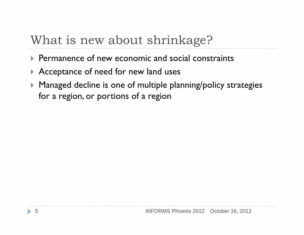
Permanence of new economic and social constraints Acceptance of need for new land uses Managed decline is one of multiple planning/policy strategies

for a region, or portions of a region

Key modeling concepts


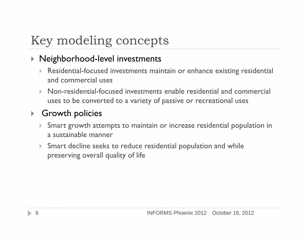
Neighborhood-level investments Residential-focused investments maintain or enhance existing residential

and commercial uses Non-residential-focused investments enable residential and commercial

uses to be converted to a variety of passive or recreational uses

Growth policies Smart growth attempts to maintain or increase residential population in

a sustainable manner Smart decline seeks to reduce residential population and while

preserving overall quality of life

Research questions


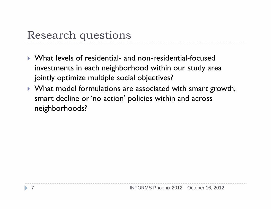
What levels of residential- and non-residential-focused investments in each neighborhood within our study area jointly optimize multiple social objectives?

What model formulations are associated with smart growth, smart decline or ‘no action’ policies within and across neighborhoods?

Modeling preliminaries


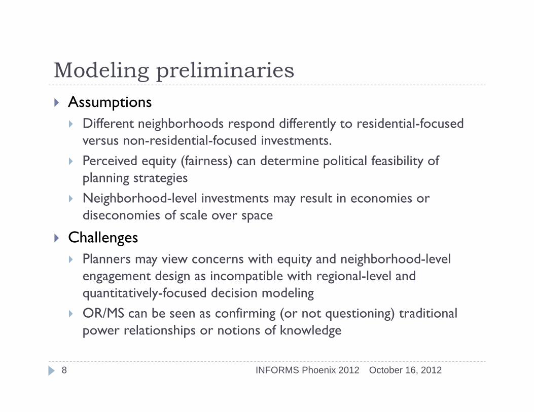
Assumptions Different neighborhoods respond differently to residential-focused

versus non-residential-focused investments. Perceived equity (fairness) can determine political feasibility of

planning strategies Neighborhood-level investments may result in economies or

diseconomies of scale over space

Challenges Planners may view concerns with equity and neighborhood-level

engagement design as incompatible with regional-level and quantitatively-focused decision modeling

OR/MS can be seen as confirming (or not questioning) traditional power relationships or notions of knowledge

Municipal shrinkage planning problem


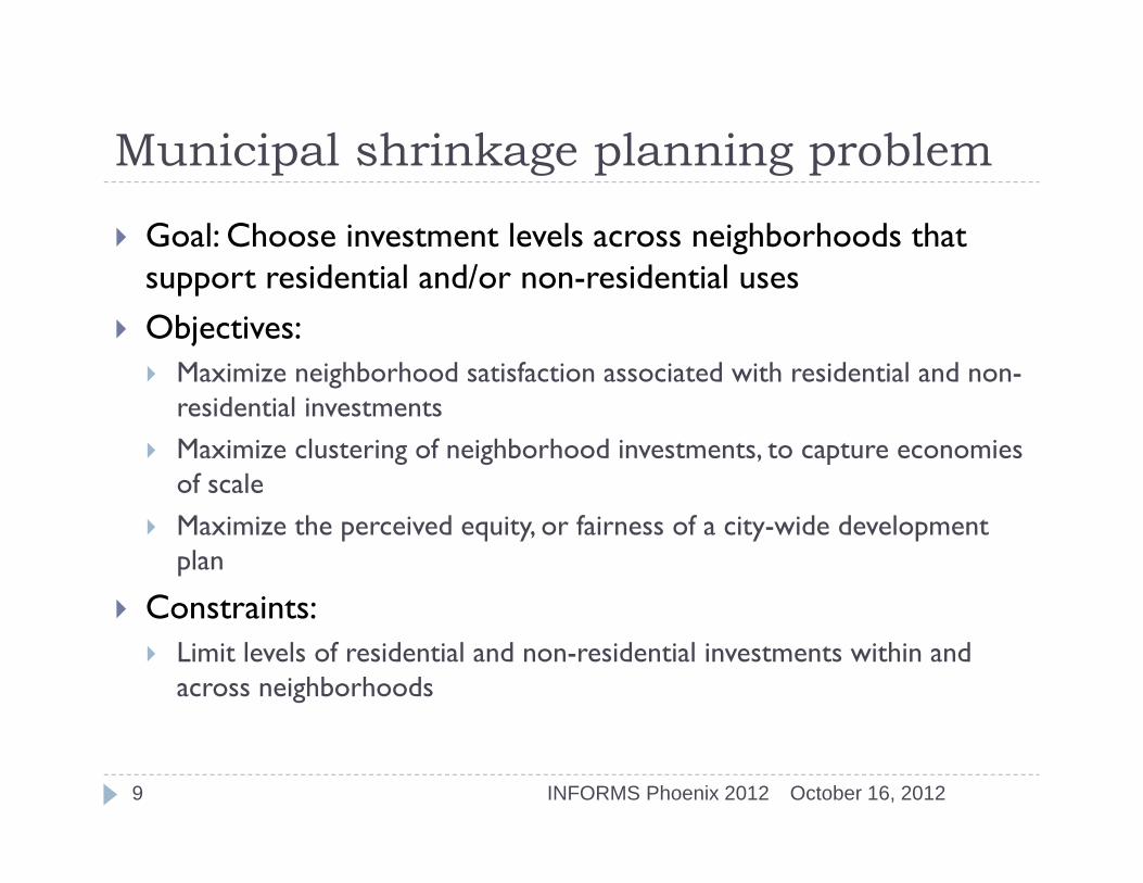
Goal: Choose investment levels across neighborhoods that support residential and/or non-residential uses

Objectives: Maximize neighborhood satisfaction associated with residential and non-

residential investments Maximize clustering of neighborhood investments, to capture economies

of scale Maximize the perceived equity, or fairness of a city-wide development

plan

Constraints: Limit levels of residential and non-residential investments within and

across neighborhoods

How can we model neighborhood satisfaction?


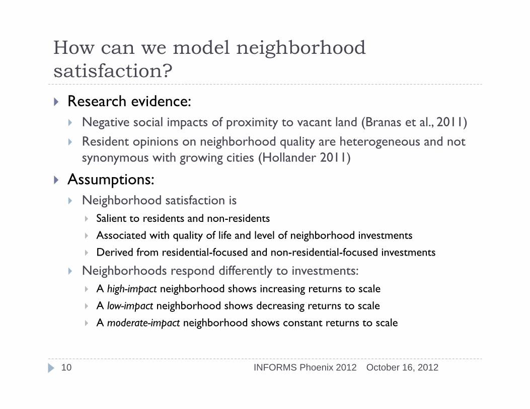
Research evidence: Negative social impacts of proximity to vacant land (Branas et al., 2011) Resident opinions on neighborhood quality are heterogeneous and not

synonymous with growing cities (Hollander 2011)

Assumptions: Neighborhood satisfaction is

Salient to residents and non-residents Associated with quality of life and level of neighborhood investments Derived from residential-focused and non-residential-focused investments

Neighborhoods respond differently to investments: A high-impact neighborhood shows increasing returns to scale A low-impact neighborhood shows decreasing returns to scale A moderate-impact neighborhood shows constant returns to scale

Neighborhood satisfaction functions


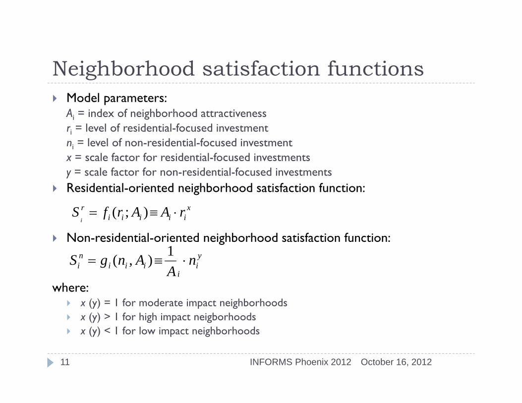
Model parameters:Ai = index of neighborhood attractivenessri = level of residential-focused investmentni = level of non-residential-focused investmentx = scale factor for residential-focused investmentsy = scale factor for non-residential-focused investments

Residential-oriented neighborhood satisfaction function:

Non-residential-oriented neighborhood satisfaction function:

where: x (y) = 1 for moderate impact neighborhoods x (y) > 1 for high impact neigborhoods x (y) < 1 for low impact neighborhoods

xiiiii

r rAArfSi

);(

yi

iiii

ni n

AAngS

1),(

Complete model


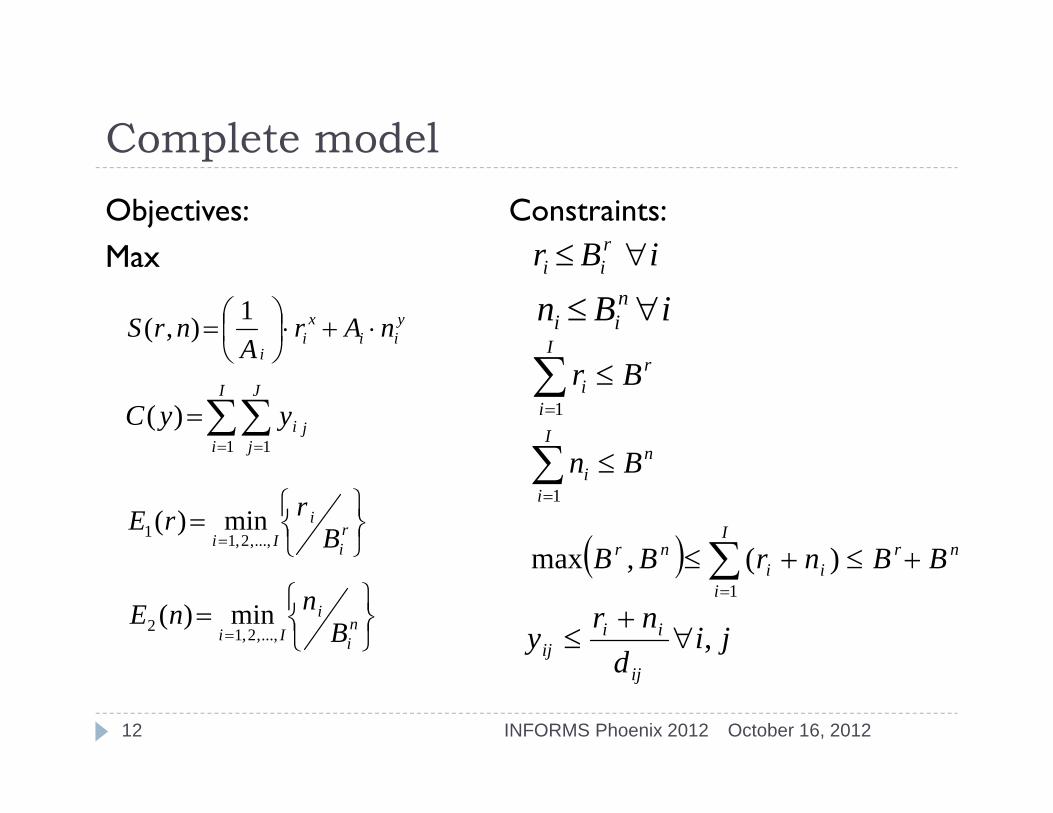
Objectives:Max

yii

xi

inAr

AnrS

1),(

I

i

J

jjiyyC

1 1)(

ri

iIi B

rrE...,,2,11 min)(

ni

iIi B

nnE...,,2,12 min)(

Constraints:iBr r

ii

iBn nii

I

i

ri Br

1

I

i

ni Bn

1

jid

nry

ij

iiij ,

nri

I

ii

nr BBnrBB

)(,max1

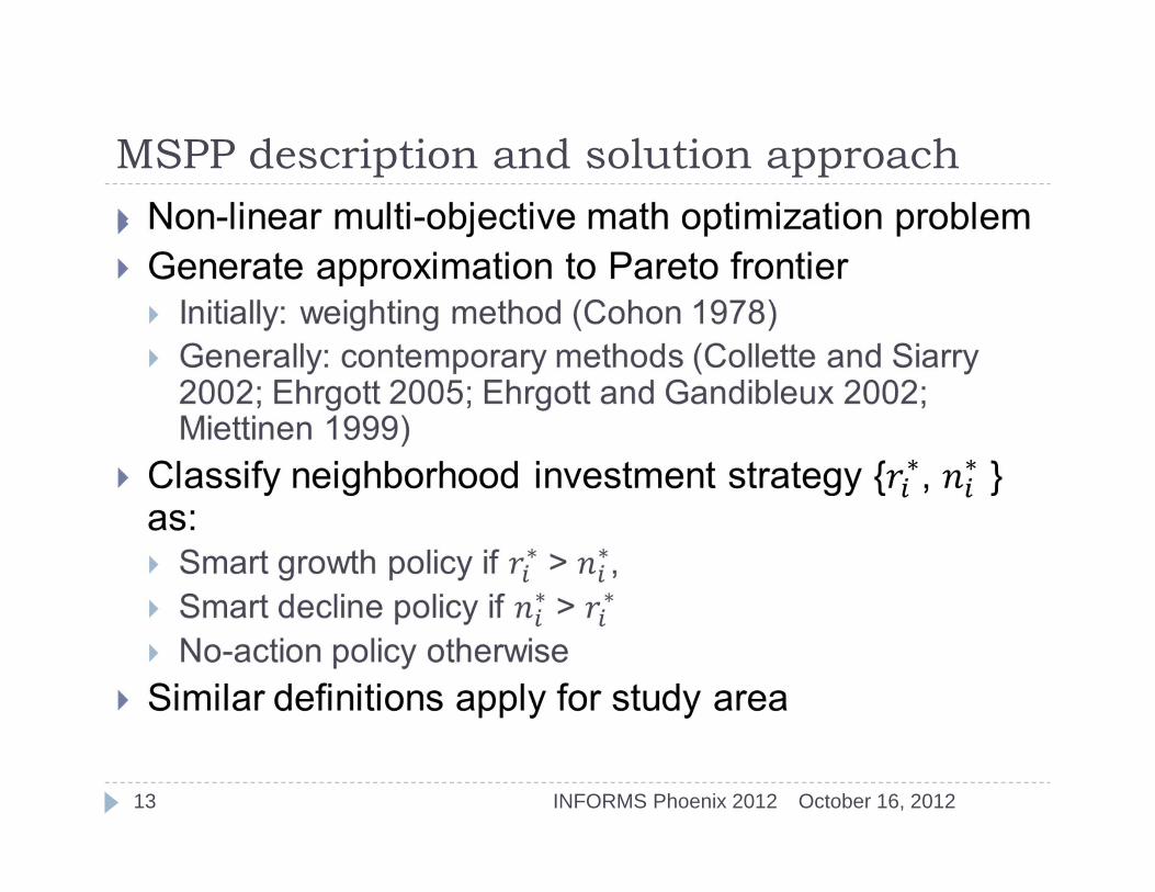
MSPP description and solution approach


Case study


Goal: apply municipal shrinkage planning problem to real city

Candidates: MA ‘gateway cities’ ‘Great’ cities Cities traditionally focus of smart decline scholarship

Method: Identify metrics of distress/decline (cf Wolff 2009) Select candidates with greatest number of distress measures

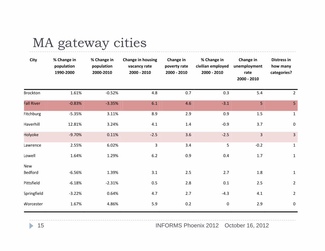
MA gateway cities


City % Change in population 1990‐2000

% Change in population 2000‐2010

Change in housing vacancy rate 2000 ‐ 2010

Change in poverty rate 2000 ‐ 2010

% Change in civilian employed

2000 ‐ 2010

Change in unemployment

rate 2000 ‐ 2010

Distress in how many categories?

Brockton 1.61% ‐0.52% 4.8 0.7 0.3 5.4 2

Fall River ‐0.83% ‐3.35% 6.1 4.6 ‐3.1 5 5

Fitchburg ‐5.35% 3.11% 8.9 2.9 0.9 1.5 1

Haverhill 12.81% 3.24% 4.1 1.4 ‐0.9 3.7 0

Holyoke ‐9.70% 0.11% ‐2.5 3.6 ‐2.5 3 3

Lawrence 2.55% 6.02% 3 3.4 5 ‐0.2 1

Lowell 1.64% 1.29% 6.2 0.9 0.4 1.7 1

New Bedford ‐6.56% 1.39% 3.1 2.5 2.7 1.8 1

Pittsfield ‐6.18% ‐2.31% 0.5 2.8 0.1 2.5 2

Springfield ‐3.22% 0.64% 4.7 2.7 ‐4.3 4.1 2

Worcester 1.67% 4.86% 5.9 0.2 0 2.9 0

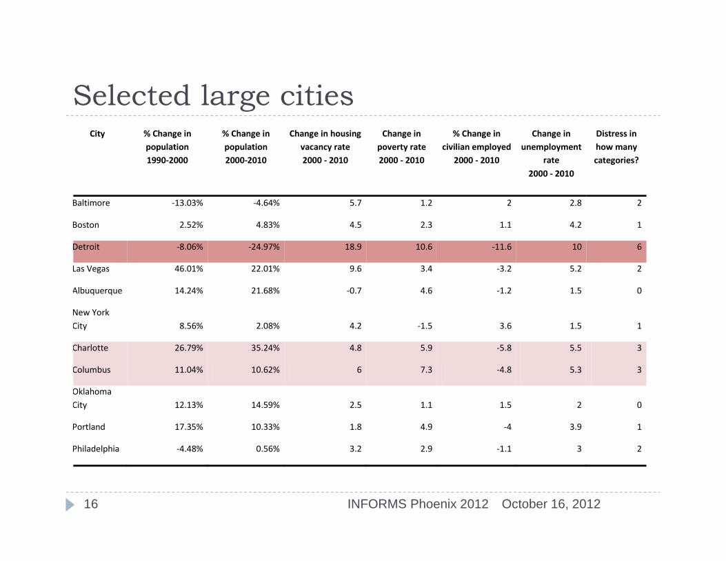
Selected large cities







2000 ‐ 2010


rate 2000 ‐ 2010


Baltimore ‐13.03% ‐4.64% 5.7 1.2 2 2.8 2

Boston 2.52% 4.83% 4.5 2.3 1.1 4.2 1

Detroit ‐8.06% ‐24.97% 18.9 10.6 ‐11.6 10 6

Las Vegas 46.01% 22.01% 9.6 3.4 ‐3.2 5.2 2

Albuquerque 14.24% 21.68% ‐0.7 4.6 ‐1.2 1.5 0

New York City 8.56% 2.08% 4.2 ‐1.5 3.6 1.5 1

Charlotte 26.79% 35.24% 4.8 5.9 ‐5.8 5.5 3

Columbus 11.04% 10.62% 6 7.3 ‐4.8 5.3 3

Oklahoma City 12.13% 14.59% 2.5 1.1 1.5 2 0

Portland 17.35% 10.33% 1.8 4.9 ‐4 3.9 1

Philadelphia ‐4.48% 0.56% 3.2 2.9 ‐1.1 3 2

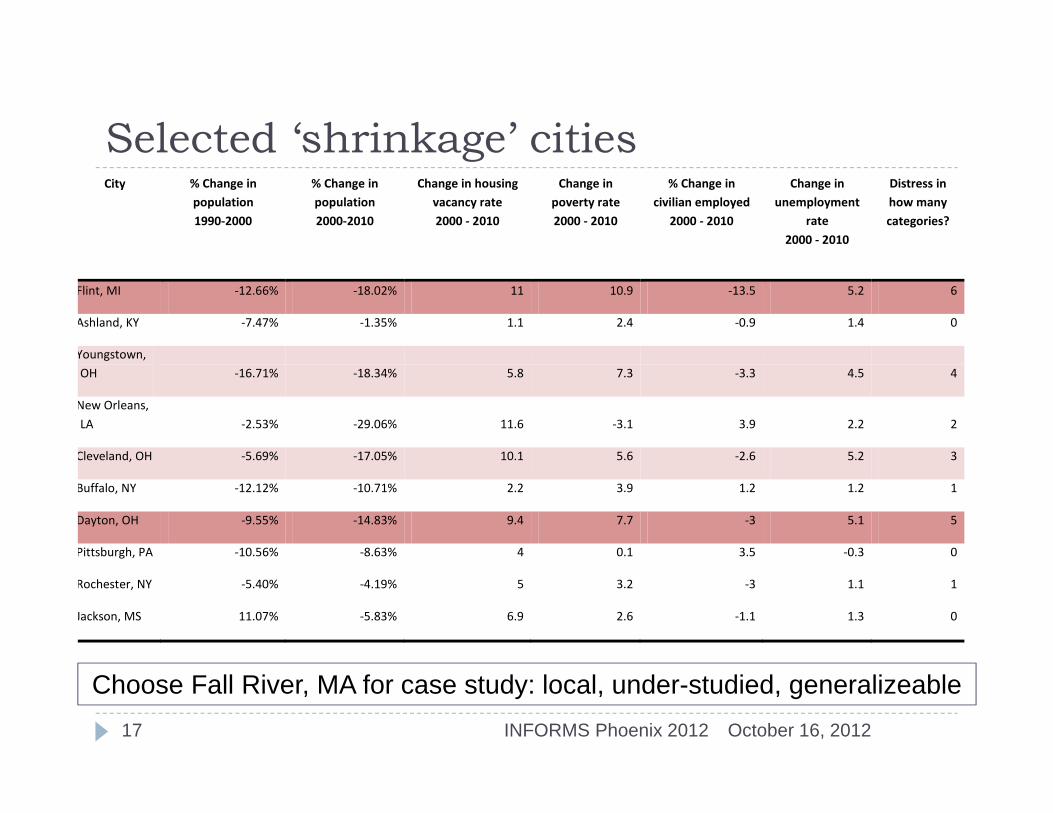
Selected ‘shrinkage’ cities







2000 ‐ 2010


rate 2000 ‐ 2010


Flint, MI ‐12.66% ‐18.02% 11 10.9 ‐13.5 5.2 6

Ashland, KY ‐7.47% ‐1.35% 1.1 2.4 ‐0.9 1.4 0

Youngstown, OH ‐16.71% ‐18.34% 5.8 7.3 ‐3.3 4.5 4

New Orleans, LA ‐2.53% ‐29.06% 11.6 ‐3.1 3.9 2.2 2

Cleveland, OH ‐5.69% ‐17.05% 10.1 5.6 ‐2.6 5.2 3

Buffalo, NY ‐12.12% ‐10.71% 2.2 3.9 1.2 1.2 1

Dayton, OH ‐9.55% ‐14.83% 9.4 7.7 ‐3 5.1 5

Pittsburgh, PA ‐10.56% ‐8.63% 4 0.1 3.5 ‐0.3 0

Rochester, NY ‐5.40% ‐4.19% 5 3.2 ‐3 1.1 1

Jackson, MS 11.07% ‐5.83% 6.9 2.6 ‐1.1 1.3 0

Choose Fall River, MA for case study: local, under-studied, generalizeable

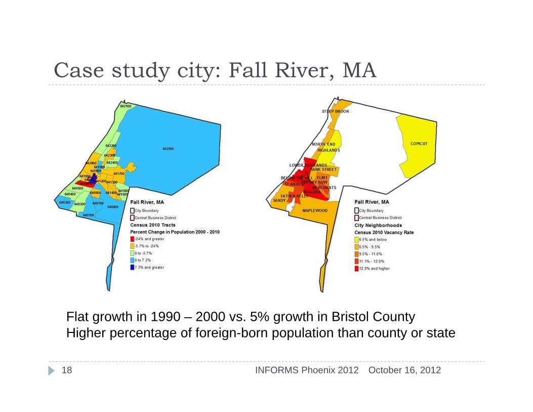
Case study city: Fall River, MA


Flat growth in 1990 – 2000 vs. 5% growth in Bristol CountyHigher percentage of foreign-born population than county or state

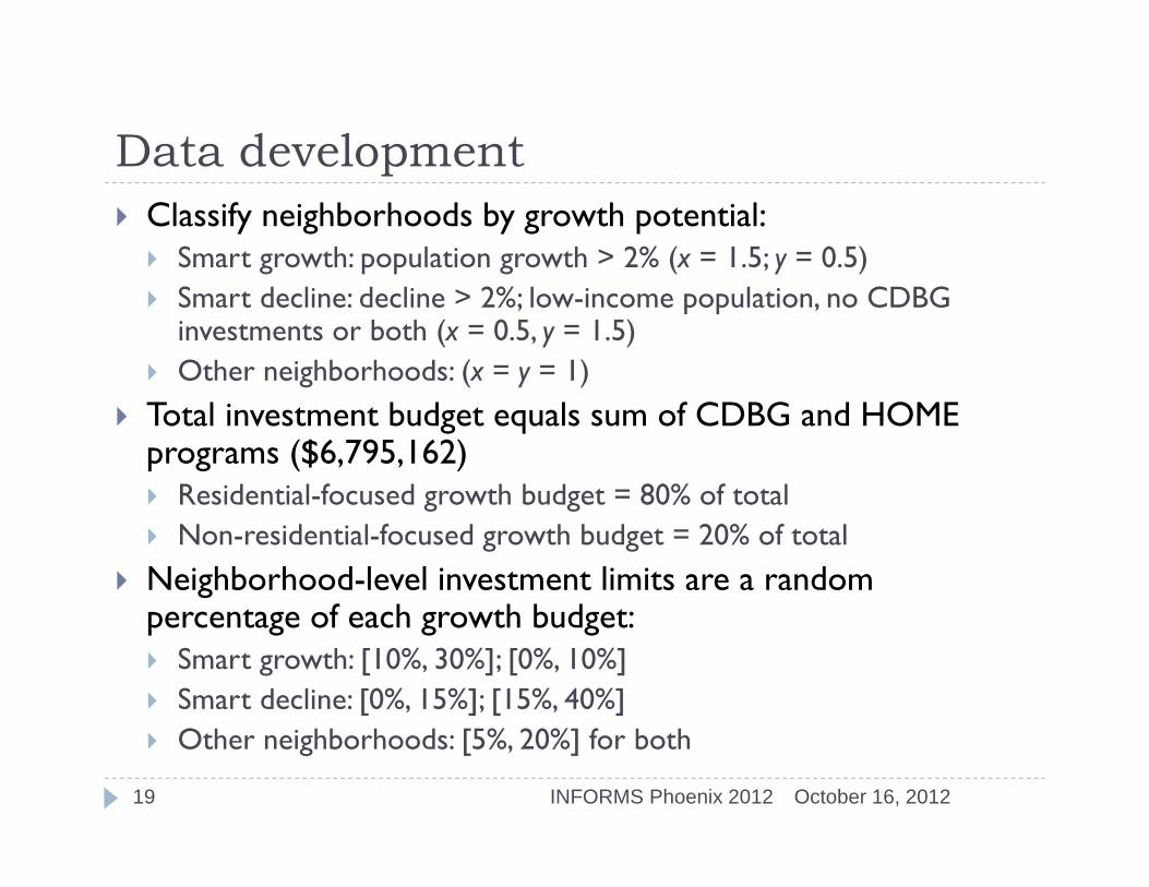
Data development


Classify neighborhoods by growth potential: Smart growth: population growth > 2% (x = 1.5; y = 0.5) Smart decline: decline > 2%; low-income population, no CDBG

investments or both (x = 0.5, y = 1.5) Other neighborhoods: (x = y = 1)

Total investment budget equals sum of CDBG and HOME programs ($6,795,162) Residential-focused growth budget = 80% of total Non-residential-focused growth budget = 20% of total

Neighborhood-level investment limits are a random percentage of each growth budget: Smart growth: [10%, 30%]; [0%, 10%] Smart decline: [0%, 15%]; [15%, 40%] Other neighborhoods: [5%, 20%] for both

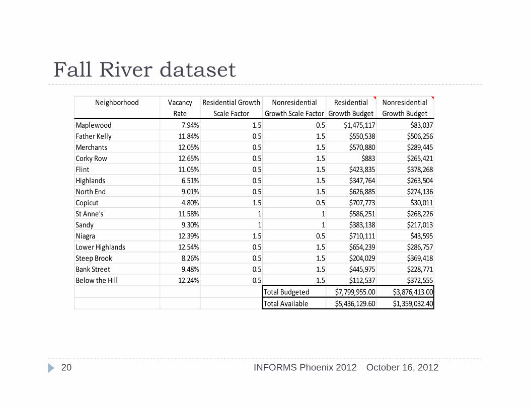
Fall River dataset


Neighborhood Vacancy Rate

Residential Growth Scale Factor

Nonresidential Growth Scale Factor

Residential Growth Budget

Nonresidential Growth Budget

Maplewood 7.94% 1.5 0.5 $1,475,117 $83,037Father Kelly 11.84% 0.5 1.5 $550,538 $506,256Merchants 12.05% 0.5 1.5 $570,880 $289,445Corky Row 12.65% 0.5 1.5 $883 $265,421Flint 11.05% 0.5 1.5 $423,835 $378,268Highlands 6.51% 0.5 1.5 $347,764 $263,504North End 9.01% 0.5 1.5 $626,885 $274,136Copicut 4.80% 1.5 0.5 $707,773 $30,011St Anne's 11.58% 1 1 $586,251 $268,226Sandy 9.30% 1 1 $383,138 $217,013Niagra 12.39% 1.5 0.5 $710,111 $43,595Lower Highlands 12.54% 0.5 1.5 $654,239 $286,757Steep Brook 8.26% 0.5 1.5 $204,029 $369,418Bank Street 9.48% 0.5 1.5 $445,975 $228,771Below the Hill 12.24% 0.5 1.5 $112,537 $372,555

Total Budgeted $7,799,955.00 $3,876,413.00Total Available $5,436,129.60 $1,359,032.40

Model solution


Premium Solver Platform using Standard LSGRG Nonlinear Engine

242 variables and 275 constraints Solution times ranged from 8.10 seconds to 32.43

seconds

Value path


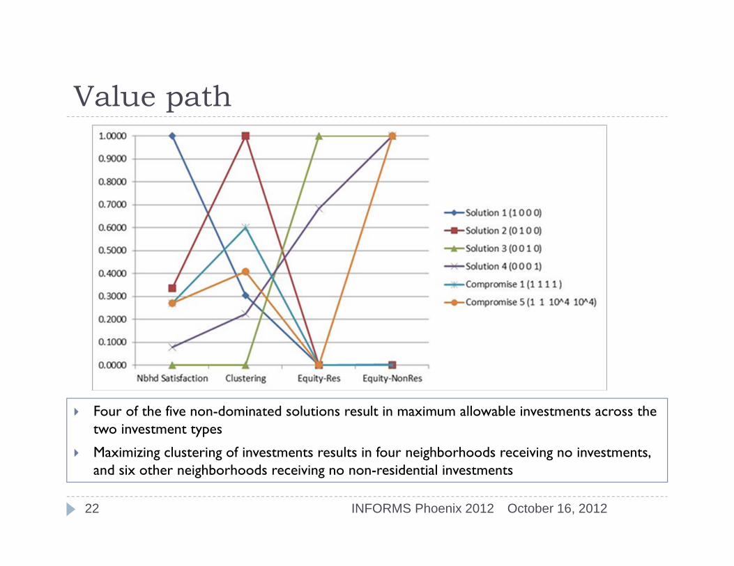
Four of the five non-dominated solutions result in maximum allowable investments across the two investment types

Maximizing clustering of investments results in four neighborhoods receiving no investments, and six other neighborhoods receiving no non-residential investments

Two non-dominated solutions – decision space


0.00

200,000.00

400,000.00

600,000.00

800,000.00

1,000,000.00

1,200,000.00

1,400,000.00

1,600,000.00

Residential Investment

Non‐Residential Investment

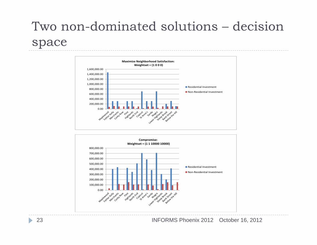
Maximize Neighborhood Satisfaction: Weightset = (1 0 0 0)

0.00

100,000.00

200,000.00

300,000.00

400,000.00

500,000.00

600,000.00

700,000.00

800,000.00

Residential Investment

Non‐Residential Investment

Compromise: Weightset = (1 1 10000 10000)

Compromise solution – decision space


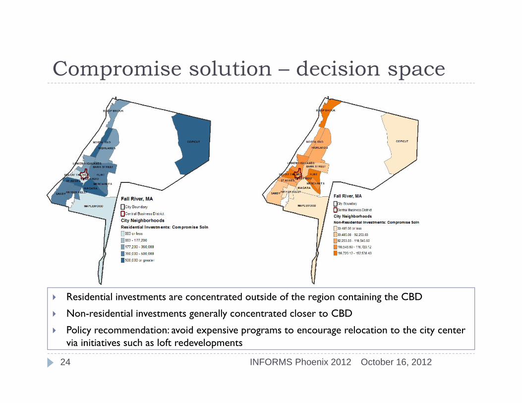
Residential investments are concentrated outside of the region containing the CBD

Non-residential investments generally concentrated closer to CBD

Policy recommendation: avoid expensive programs to encourage relocation to the city center via initiatives such as loft redevelopments

Analysis of solutions


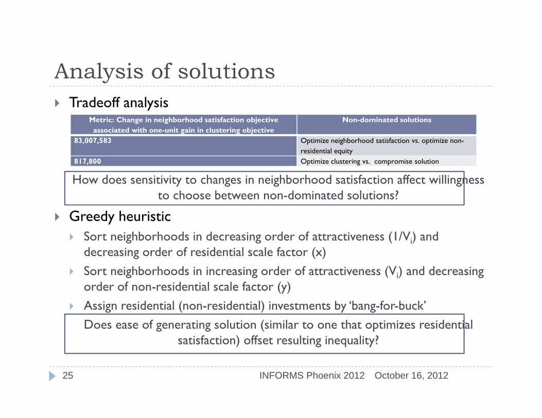
Tradeoff analysis

How does sensitivity to changes in neighborhood satisfaction affect willingness to choose between non-dominated solutions?

Greedy heuristic Sort neighborhoods in decreasing order of attractiveness (1/Vi) and

decreasing order of residential scale factor (x) Sort neighborhoods in increasing order of attractiveness (Vi) and decreasing

order of non-residential scale factor (y) Assign residential (non-residential) investments by ‘bang-for-buck’

Does ease of generating solution (similar to one that optimizes residential satisfaction) offset resulting inequality?

Metric: Change in neighborhood satisfaction objective associated with one-unit gain in clustering objective

Non-dominated solutions

83,007,583 Optimize neighborhood satisfaction vs. optimize non-residential equity

817,800 Optimize clustering vs. compromise solution

Conclusions


Initial effort to provide tangible and substantive guidance to planners and policy-makers

Solutions balance neighborhood satisfaction, economic efficiency and social equity while accommodating practical limitations on neighborhood-level resource availability

Neighborhood satisfaction model incorporates notions of scale economies of neighborhood investments while distinguishing between traditional and non-traditional uses

Non-dominated solutions can serve as a basis for community discussions but not intended to generate specific planning prescriptions

Next steps


Current model Emiprically model and validate neighborhood satisfaction functions Investigate alternative forms for equity function Convert decision model to MOLP Enagage actual client and allow for different modeling and solution

approaches

Alternative decision problems Target individual residential parcels for continued occupancy or allow to

become vacant Select vacant parcels for investment for alternative uses

Questions?


Documents

Maintain, Demolish, Re‐purpose: Policy Design for Vacant