Embed Size (px)
Citation preview

Magnetic Resonance Imaging
�(r) = Z S(k)e�i2�k�rB 0
Thomas Vosegaard
Laboratory for Biomolecular NMR SpectroscopyDepartment of Molecular Biology and Interdisciplinary Nanoscience Center
University of Aarhus
November 2005

Preface
These Notes intend to give a short introduction to mag-
netic resonance imaging (MRI). MRI represents a very
hot topic within medical sciences as evidenced by the
2003 Nobel Price in medicine awarded to the founders
of MRI, Paul Lautherbur and Peter Mansfield.
The first Sections summarize basic NMR theory. It may
be well-known stuff and serves primarily to present the
entire theory needed to understand MRI in the same no-
tation as applied for the following imaging Sections.
From Section 6 and onwards the basic concepts of MRI
are explained, and pulse sequences routinely applied on
MR scanners worldwide are presented.
I hope these Notes contribute to your understanding of
imaging and that you, after reading them, share my fasci-
nation for MRI.
I would like to thank Anders Malmendal for many valu-
able comments on these Notes.
Thomas Vosegaard

CONTENTS iii
Contents
1 Nuclear Spin Interactions 1
1.1 Nuclear Magnetic Moment and Nuclear Spin . . . . . 1
1.2 The Zeeman Interaction . . . . . . . . . . . . . . . . 2
1.3 The Magnetization of the Sample . . . . . . . . . . . . 3
1.4 Nuclear Spin Interactions . . . . . . . . . . . . . . . . 4
1.4.1 Chemical Shift . . . . . . . . . . . . . . . . . 4
1.4.2 Spin-Spin Coupling . . . . . . . . . . . . . . . 4
2 Aspects of One-Dimensional NMR 7
2.1 Manipulation of the Nuclear Magnetization . . . . . . 8
2.1.1 Detection of the Free-Induction Decay . . . . . 9
2.2 The Rotating Frame of Reference . . . . . . . . . . . . 9
2.3 Radio-Frequency Pulses . . . . . . . . . . . . . . . . 11
2.3.1 The Single-Pulse Experiment . . . . . . . . . 13
2.3.2 The Spin-Echo Experiment . . . . . . . . . . . 13
3 Relaxation 17
3.1 Longitudinal Relaxation, T1 . . . . . . . . . . . . . . 17
3.2 Transverse Relaxation, T2 and T2⋆ . . . . . . . . . . . 20
4 Fourier Transformation 22
4.1 One-Dimensional Fourier Transformation . . . . . . . 22
4.2 Discrete Fourier Transformation . . . . . . . . . . . . 24
4.3 Two-Dimensional Fourier Transformation . . . . . . . 24
5 Basic Two-Dimensional NMR 27
6 Magnetic Field Gradients 27
6.1 The Gradient Echo . . . . . . . . . . . . . . . . . . . 28

iv CONTENTS
7 Principles of Magnetic Resonance Imaging 28
7.1 Selective Radio-Frequency Irradiation . . . . . . . . . 30
7.2 Slice Selection . . . . . . . . . . . . . . . . . . . . . 31
8 k-Space Imaging 33
8.1 Acquiringk-Space Data . . . . . . . . . . . . . . . . 34
8.2 Practical Aspects ofk-Space Imaging . . . . . . . . . 37
8.3 Fast Imaging Techniques . . . . . . . . . . . . . . . . 39
8.3.1 Echo Planar Imaging . . . . . . . . . . . . . . 42
8.3.2 Spiral Imaging . . . . . . . . . . . . . . . . . 42
8.3.3 Comparison of Spiral and Echo-Planar Imaging 44
8.4 Image Contrast . . . . . . . . . . . . . . . . . . . . . 47
8.5 T1-Weighted Imaging . . . . . . . . . . . . . . . . . . 47
8.6 T2- and T2⋆-Weighted Imaging . . . . . . . . . . . . . 49
8.7 Creating Contrast Using Contrast Agents . . . . . . . . 50
9 Functional Imaging 51
10 Magnetic-Resonance Angiography 55
10.1 Time-of-Flight MRA . . . . . . . . . . . . . . . . . . 55
10.2 Phase-Contrast MRA . . . . . . . . . . . . . . . . . . 56
11 Localized Magnetic Resonance Spectroscopy 56
11.1 Single-Voxel Techniques . . . . . . . . . . . . . . . . 58
11.2 Multi-Voxel Techniques . . . . . . . . . . . . . . . . . 58
12 Instrumentation 60
12.1 MR Scanners . . . . . . . . . . . . . . . . . . . . . . 60
12.2 Gradient System . . . . . . . . . . . . . . . . . . . . . 62

1 NUCLEAR SPIN INTERACTIONS 1
1 Nuclear Spin Interactions
The physical principle that forms the basis for nuclear magnetic res-
onance (NMR) and magnetic resonance imaging (MRI) is the inter-
action between atomic nuclei with nonzero spin and a magnetic field.
This concept was first postulated in the 1920s by the WolfgangPauli,
but was not experimentally demonstrated until 1946 when Felix Bloch
and Edward Purcell ran the first NMR spectra. Bloch and Purcell were
awarded the Nobel price in 1952 for their achievements.
1.1 Nuclear Magnetic Moment and Nuclear Spin
The atomic nucleus consists of protons and neutrons and is positively
charged. If the nucleus spins about its own axis, it will generate a
magnetic field similarly to an electric current flowing in theloop of a
circular wire. This field is termed thenuclear magnetic dipole. The
magnetic dipole will interact with external magnetic fieldsjust like a
compass needle interacts with the magnetic field of the Earth.
Thenuclear spindescribes the fact that some nuclei interact with
external magnetic fields like a rotating top that not only rotates about
its own axis but may be perturbed so its rotation axis precesses around
the Earth’s gravitational field. Thus, the nuclear spin may be repre-
sented by a vector aligned along the precession axis. For thenucleus
the precession frequency,ω0, is proportional to the external magnetic
field B0 as
ω0 = γB0 (1)
where the constant of proportionality,γ, is termed the gyromagnetic
ratio and is a fundamental property for every isotope.
Only atomic nuclei with unpaired protons or neutrons possess a

2 1.2 The Zeeman Interaction
Table 1: Nuclear spin, natural abundance, and gyromagnetic ratiosfor some typical isotopes
Atom Spin Natural Gyromagn. ratio Biologicalabundance (%) γ/2π (MHz/T) density (%)
1H 1/2 99.985 42.58 1013C 1/2 1.108 10.71 2315N 1/2 0.37 4.32 2.619F 1/2 100 40.07 0.0431P 1/2 100 17.24 1.1
nuclear spin. The nuclear spinI is the number of unpaired nuclear
particles times 1/2. In this text we will focus on isotopes with nu-
clear spinI = 1/2, of which some are listed in Table 1. The nuclear
spin number,I, is often termed thenuclear spin quantum numberand
represents the length of the spin vector.
1.2 The Zeeman Interaction
When a nucleus possessing a nuclear spin is placed in a magnetic field
(in NMR and MRI the magnetic field is normally defined to be par-
allel to thez axis), thez component of the nuclear spin,Iz , becomes
quantitized and only takes discrete values of
Iz = −I,−I + 1, ..., I. (2)
In the case of spin-1/2 nucleiIz takes the values−1/2 and1/2, typi-
cally referred to asβ andα.
The different states arise because of the interaction between the
nuclear spin and the external magnetic field. This interaction was first
characterized by Pieter Zeeman and is therefore dubbed the Zeeman
interaction. The energy of the individual levels are given by

1 NUCLEAR SPIN INTERACTIONS 3
E = −~ω0Iz . (3)
1.3 The Magnetization of the Sample
The population of theα andβ spin states of a large number of spins
present in a macroscopic sample is determined by the temperature. At
very low temperature, all spins will be in the low-energy state while at
higher temperatures there will be some thermal excitation to the high-
energy state. This was originally described by Ludwig Boltzmann and
is normally called the Boltzmann distribution. It states that the macro-
scopic distribution of particles over the energy levels is exponentially
decreasing,
Nβ
Nα
= exp
{
−Eβ − Eα
kT
}
≈ 1 −~ω0
kT, (4)
with k representing the Boltzmann constant andT being the absolute
temperature of the sample. The last approximation is a powerex-
pansion1 using the fact that for NMR the energy difference is much
smaller thankT .
The fact that theα andβ states are differently populated creates a
macroscopic magnetization of the sample. At equilibrium, this mag-
netization will be aligned along the magnetic field, i.e., itmay be rep-
resented by a vector,M eq = M z, pointing along the magnetic field
(z).
Since the energy difference between two spin states is very small,
e.g. as compared to the energies present in vibrational or electronic
spectroscopy, the termodynamic preference for the state with lower
1A power expansion is an approximation where a complicated function,f(x), maybe approximated by the functionf(x) = f(x0) + f ′(x0)(x − x0) + ..., for values ofx in the vicinity ofx0.

4 1.4 Nuclear Spin Interactions
energy is not very large. With the NMR signal being proportional
to the population difference (Nα − Nβ) NMR has a relatively low
sensitivity compared to other spectroscopic techniques. For example,
the population difference between protons in theα andβ states at 1.5
T is about10−5.
1.4 Nuclear Spin Interactions
A number of different nuclear spin interactions makes NMR spec-
troscopy a very informative disciplin, capable of providing important
structural and dynamic information. Below we will briefly summarize
two of these interactions and the type of information they may provide.
1.4.1 Chemical Shift
Just like the nucleus creates a small magnetic field due to itsrotation,
electrons circling around the nucleus in different orbitals will gener-
ate a magnetic field. This field is in opposite direction to theexternal
magnetic field resulting in a diminished effective magneticfield at the
position of the nucleus. This phenomenon, known as chemicalshield-
ing, is illustrated in Fig. 1a.Shieldingbecause the electrons diminish
the field and thereby ”shield” the nucleus andchemicalbecause the
shielding depends on the chemical environment of the particular atom
studied.
1.4.2 Spin-Spin Coupling
As discussed in Section 1.1, a nucleus creates a small magnetic field
which, according to Section 1.2, either is aligned along or against the
external magnetic field. Close to the nuclear spin, the effective mag-
netic field will then be either larger or smaller thanB0 depending on
the spin state (α or β) of the nucleus as illustrated in Fig. 1b. A second

1 NUCLEAR SPIN INTERACTIONS 5
effB 0=B0B
effB 0= B
effB 0= B
n+ B
n− B
B n
0B
(1−σ)
a
bB n
Figure 1: Illustration of the effect of chemical shielding and spin-spin couplings. (a) Compared to the external magnetic field B0,the nucleus will sense a smaller magnetic field due to the shieldingof the surrounding electrons. (b) A nearby spin will create a netmagnetization parallel or antiparallel to B0 causing a change in theeffective field at the position of the observed nucleus.

6
ppm2345
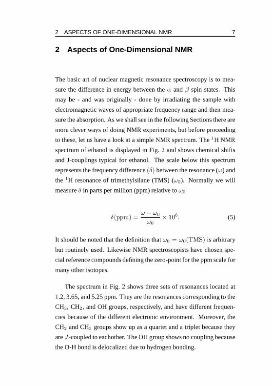
Figure 2: 1H NMR spectrum of ethanol.
nucleus placed in the vicinity of the first nucleus will then have a reso-
nance frequency depending on the spin state of the first nucleus. This
is referred to as a coupling between the nuclei. The most common
type of coupling in liquids is theJ-coupling that is mediated through
covalent bonds.
Since the Boltzmann distribution only causes a marginal difference
in the population of theα andβ states, the coupling between two nu-
clei will make each of their resonance split into two lines ofvirtually
equal intensity corresponding to the two spin states of the neighbour-
ing spin.
2 ASPECTS OF ONE-DIMENSIONAL NMR 7
2 Aspects of One-Dimensional NMR
The basic art of nuclear magnetic resonance spectroscopy isto mea-
sure the difference in energy between theα andβ spin states. This
may be - and was originally - done by irradiating the sample with
electromagnetic waves of appropriate frequency range and then mea-
sure the absorption. As we shall see in the following Sections there are
more clever ways of doing NMR experiments, but before proceeding
to these, let us have a look at a simple NMR spectrum. The1H NMR
spectrum of ethanol is displayed in Fig. 2 and shows chemicalshifts
and J-couplings typical for ethanol. The scale below this spectrum
represents the frequency difference(δ) between the resonance (ω) and
the 1H resonance of trimethylsilane (TMS) (ω0). Normally we will
measureδ in parts per million (ppm) relative toω0
δ(ppm) =ω − ω0
ω0
× 106. (5)
It should be noted that the definition thatω0 = ω0(TMS) is arbitrary
but routinely used. Likewise NMR spectroscopists have chosen spe-
cial reference compounds defining the zero-point for the ppmscale for
many other isotopes.
The spectrum in Fig. 2 shows three sets of resonances locatedat
1.2, 3.65, and 5.25 ppm. They are the resonances corresponding to the
CH3, CH2, and OH groups, respectively, and have different frequen-
cies because of the different electronic environment. Moreover, the
CH2 and CH3 groups show up as a quartet and a triplet because they
areJ-coupled to eachother. The OH group shows no coupling because
the O-H bond is delocalized due to hydrogen bonding.

8 2.1 Manipulation of the Nuclear Magnetization
Theory Box 1: The Bloch Equations
The nuclear magnetization may be ma-
nipulated by external magnetic fields
with orientations perpendicular to the
magnetization vector,M. Likewise the
magnetic field will be represented by the
vector B, and thusB0 = (0, 0, B0).
The magnetization vector obeys a dif-
ferential equation, the socalled Bloch
equation, constructed in 1948 by Felix
Bloch,
dMx
dt= γ(MyBz − MzBy)
dMy
dt= γ(MzBx − MxBz)
dMz
dt= γ(MxBy − MyBx)
(T1-1)
If B = B0(= Bz), the solution to
these differential equations is
Mx(t) =
M0x cos(ω0t) − M0
y sin(ω0t)
My(t) =
M0y cos(ω0t) + M0
x sin(ω0t)
Mz(t) = M0z
(T1-2)
whereω0 = γB0. This shows that if
there were initial transverse (x and y)
components of the magnetization vec-
tor, they would precess around the exter-
nal magnetic field with the larmor fre-
quency, while the longitudinal (z) com-
ponent will remain unaltered.
2.1 Manipulation of the Nuclear Magnetization
Theory Box 1 demonstrates how the macroscopic magnetization of
the sample may be manipulated by external magnetic fields, and it
is demonstrated that the magnetic field must be perpendicular to the
magnetization to have any effect. Moreover, the concepts oflongitu-
dinal and transverse magnetization are introduced in Theory Box 1.
These terms represent the magnetization components alongz and in
thexy plane, respectively. As we shall see later, and as it is also ap-
parent from Eq. T1-2 in Theory Box 1 there is a physical basis for this
distinction.
We may use the behaviour of the Bloch equations to manipulatethe
orientation of the magnetization by applying small magnetic fields in
other directions. Equation T1-1 in Theory Box 1 states that whenever

2 ASPECTS OF ONE-DIMENSIONAL NMR 9
the magnetization vector experiences a magnetic field perpendicular to
its orientation, it will start to precess around the axis of the magnetic
field. Suppose we in addition to theB0 field apply a small field,B1,
alongx. This will just create an effective field slightly tilted away from
z in thexz plane and the magnetization will start to precess around this
new effective field axis. On the other hand, if theB1 field oscillates
in thexy plane with a frequency ofω0, it may be kept perpendicularly
to M at all times and tilt the magnetization away fromz. This is
illustrated in Fig. 3a on page 12 and will be treated more thoroughly
in Section 2.3.
2.1.1 Detection of the Free-Induction Decay
It is well-known, e.g. from electrical transformators, that just like an
alternating current in a coil will create an alternating magnetic field, an
alternating magnetic field is able to generate an alternating current in
a coil. Thus, the oscillating magnetic field caused by the precession of
the transverse component of the magnetization of the samplemay be
detected as an alternating current in a coil wrapped around the sample.
In practice, we will measure the NMR signal,S, in this manner by
measuring both thex andy components of the free-induction decay.
This means that the harmonically oscillating signal may be described
by the complex functionS(t) = exp{iωt}.2
2.2 The Rotating Frame of Reference
You probably find it much easier to denominate resonance frequencies
by e.g., 1 ppm as on the scale in Fig. 2 instead 400.0004, etc. The
scale below the spectrum is a ppm scale calculated by Eq. 5.
2A complex number (c) has a real (x) and an imaginary (y) part,c = x + iy, wherei is the complex numberi =
√−1. The complex exponential function is represented
by the harmonic oscillators,exp{iωt} = cos ωt + i sin ωt.

10 2.2 The Rotating Frame of Reference
Theory Box 2: The Rotating Frame
As evidenced in Theory Box 1 any
transverse magnetization will rotate
with the larmor frequency around thez
axis. In our normal representation of
NMR spectra (see e.g., Fig. 2 we use
the ppm scale which represents the ac-
tual resonance frequency minus the lar-
mor frequency. Likewise, when observ-
ing the evolution of the magnetization in
a coordinate system, it is convenient to
use a frame where the larmor frequency
is subtracted. This corresponds to trans-
ferring the description of into a frame
rotating at the larmor frequency around
z. This frame will be denotedx′, y′,
and z. The relation between the two
frames is as follows:
x′ = x cos ω0t + y sinω0t
y′ = y cos ω0t − x sinω0t (T2-1)
When depicting the oscillation of the magnetization vectorin a
three-dimensional coordinate system it is also simpler to omit the lar-
mor frequency and only depict the small variations in the resonance
frequencies relative to the larmor frequency. For details on the mathe-
matical way of handling this, see Theory Box 2.
In popular terms, the philosophy of the rotating frame is like a
carousel in an amusement park. If you want to talk to the people who
are on the carousel it is most convenient to step onto the carousel than
staying next to it.
In the NMR spectrometer or MR imaging scanner, the signal in the
rf coil generated by the sample consists of as a high-frequency (ω0)
signal with small frequency modulations (δ) due to the nuclear spin
interactions. This is in full analogy to the principle of normal FM ra-
dios where the signal of interest (audio signal) representsa modulation
of a high-frequency carrier of around 100 MHz. In NMR and MRI the
signal from the coil is passed through a frequency mixer which cre-
ates the difference signalω − ω0, which exactly corresponds to the
description in the rotating frame.

2 ASPECTS OF ONE-DIMENSIONAL NMR 11
The radio frequency of the mixer is often referred to as the car-
rier frequency and needs not be identical to the Larmor frequencyω0.
However, to keep the notation simple in these notes we will also use
the termω0 as the carrier frequency.
2.3 Radio-Frequency Pulses
As previously mentioned the nuclear magnetization will interact with
external magnetic fields. If the additionalB1 field rotates in thexy
plane with the resonance frequency (ω0), it appears static in the rotat-
ing frame, e.g. along thex′ axis, and will always be perpendicular to
M. Consequently this field makes the magnetization begin to precess
around theB1 (x′) axis. The effect of this is visualized in Fig. 3 as
observed in the laboratory (a) and rotating (b) frames. Becauseω0
lies in the radio-frequency range of the electromagnetic spectrum, the
oscillatingB1 field will be a referred to as a radio-frequency (rf) field.
Like large magnetic field,B0, the small oscillating field will make
the magnetization vector precess with a frequency ofω1 = γB1. For
most NMR and MRI experimentsω1 will be in the kHz range.
If we want to bring the sample from its thermal equilibrium state
(Mz) to a state with transverse magnetization in order to detectthe
NMR signal, we may apply theB1 field for exactly the period of time
it takes to perform a 90◦ (π/2) rotation of the magnetization vector
aroundx′. Such short periods of rf irradiation are referred to as rf
pulses and the rotation angle is called the flip-angle. The flip angle of
the pulse is given byθ = ω1t and hence
t90◦ =π
2ω1
. (6)
The concept of pulsed NMR spectroscopy was developed by Richard
R. Ernst in the 1960s, an effort for which he was awarded the Nobel

12 2.3 Radio-Frequency Pulses
a
b
y’
x’
Figure 3: Evolution of the nuclear spin magnetization in the labo-ratory frame (a) and in the rotating frame (b) in the presence of anexternal field, B0, and a transverse rotating field, B1.

3 RELAXATION 13
price in 1991. In the following Sections it will be demonstrated how
pulse sequences may be used to manipulate the spin system andto
bring it to a desired state.
2.3.1 The Single-Pulse Experiment
The most simple pulsed NMR experiment one may think of consists
of a 90◦ pulse that flips the equilibrium magnetizationMz to an ori-
entation in the transverse plane (e.g. along thex′ axis) for detection as
illustrated in Fig. 4a. If all spins were precessing with exactly ω0 there
would be no further evolution in the rotating frame and the spin system
would stay in the state shown in Fig. 4b (in practice there will be an
exponential decay due to relaxation as discussed in Section3). How-
ever, if there are different spins the magnetization vectors for these
spins (e.g. as labelled 1-4 in Fig. 4c) will start to precess with fre-
quences determined by the nuclear spin interactions. Upon detection
the free-induction decay may be transformed from the time domain
into a spectrum like the one in Fig. 2.
2.3.2 The Spin-Echo Experiment
The spin-echo experiment shown in Fig. 5 uses the following sequence
of pulses and delays:90◦y−τ−180◦x−τ . After the first pulse and delay,
the different species will have obtained ax′y′ phase encoding,θi =
(ωi − ω0)τ , due to their different resonance frequencies. The 180◦
pulse brings magnetization alongx′ to −x′ and z to −z, changing
thex′y′ phases fromθi −→ −θi. Consequently, after a second delay
of durationτ all spins will be refocussed and a socalled spin echo is
formed.

14
TR TR
b
y
θ3
za b z
x’
y’
x’
y’
z
1
3
4
2x’
y’
c
a c
Figure 4: Rotating-frame vector representation of the evolution ofthe magnetization before and after a pulse using the displayedpulse sequence. (a) Before the 90◦ pulse the magnetization is atthermal equilibrium aligned along the external magnetic field. (b)The pulse flips the magnetization from z to x′. When being in thetransverse plane, the magnetization vectors for different spins startto precess with different frequencies due to their chemical shift. Ata certain time, t, the individual species have obtained different x′y′
phases given by θi(t) = (ωi − ω0)t. To improve the S/N ratio theexperiment will typically be repeated several times with a repetitiondelay of TR as shown on the top.

3 RELAXATION 15
ze
x’
y’
za b
x’
y’
z
x’
y’
a b c d
τ τ
TEey x
z
1
3
4 4
2
1
3
zc d
2x’
y’
x’
y’
Figure 5: Rotating-frame vector representation of the evolution ofthe magnetization during a spin-echo experiment as displayed bythe pulse sequence on the top. (a) An initial 90◦ pulse flips the mag-netization from z to x′ (b). (c) After a delay τ the different specieshave obtained x′y′ phases due to their different chemical shift. (d)A 180◦
x pulse is applied to the spins in (c) and they undergo thetransformation y′
−→ −y′, z −→ −z. (e) After a second delay τall spins are refocussed to lie along x′. If no transverse relaxationwere present this situation would correspond to the spin state in (a).The time elapsed from the initial pulse to the formation of the echois called TE.

16
Theory Box 3: The Modified Bloch Equations
The differential equations describing
the evolution of the magnetization vec-
tor in the presence of an external mag-
netic field, the socalled Bloch equations
(Eq. T1-1 in Theory Box 1) represents
the ideal behaviour of the magnetization
vector in the presence of external mag-
netic fields. However, as we mentioned
above the system studied will be influ-
enced by relaxation, which is a physical
phenomenon that makes the system re-
turn from an excited state to its equilib-
rium state. The Bloch equation (Eq. T1-
1) may be extended to include this ef-
fect, resulting in a new set of differential
equations, normally dubbed the modi-
fied Bloch equations
dMx
dt= γ(MyBz − MzBy)
−Mx/T2
dMy
dt= γ(MzBx − MxBz)
−My/T2 (T3-1)
dMz
dt= γ(MxBy − MyBx)
+Mz/T1,
in which case the solution for the trans-
verse components of the magnetization
become
Mx(t) =`
M0x cos(ω0t) − M0
y sin(ω0t)´
× exp(−t/T2).(T3-2)
The latter equation in Eq. T3-1 tells
us that the longitudinal component of
the magnetization vector will return to
the equilibrium state via an exponential
growth (1 − exp(−t/T1)), in analogy
to the decay of the transverse magneti-
zation.
3 RELAXATION 17
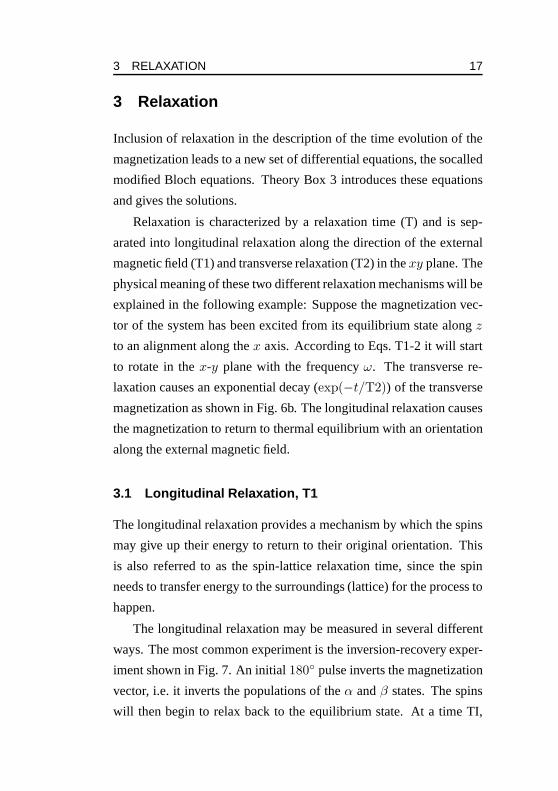
3 Relaxation
Inclusion of relaxation in the description of the time evolution of the
magnetization leads to a new set of differential equations,the socalled
modified Bloch equations. Theory Box 3 introduces these equations
and gives the solutions.
Relaxation is characterized by a relaxation time (T) and is sep-
arated into longitudinal relaxation along the direction ofthe external
magnetic field (T1) and transverse relaxation (T2) in thexy plane. The
physical meaning of these two different relaxation mechanisms will be
explained in the following example: Suppose the magnetization vec-
tor of the system has been excited from its equilibrium statealongz
to an alignment along thex axis. According to Eqs. T1-2 it will start
to rotate in thex-y plane with the frequencyω. The transverse re-
laxation causes an exponential decay (exp(−t/T2)) of the transverse
magnetization as shown in Fig. 6b. The longitudinal relaxation causes
the magnetization to return to thermal equilibrium with an orientation
along the external magnetic field.
3.1 Longitudinal Relaxation, T1
The longitudinal relaxation provides a mechanism by which the spins
may give up their energy to return to their original orientation. This
is also referred to as the spin-lattice relaxation time, since the spin
needs to transfer energy to the surroundings (lattice) for the process to
happen.
The longitudinal relaxation may be measured in several different
ways. The most common experiment is the inversion-recoveryexper-
iment shown in Fig. 7. An initial180◦ pulse inverts the magnetization
vector, i.e. it inverts the populations of theα andβ states. The spins
will then begin to relax back to the equilibrium state. At a time TI,

18 3.1 Longitudinal Relaxation, T1
Mz
Mxy
Time
Time
a
b
Inte
nsity
,In
tens
ity,
Small T2
Large T1
Small T1
Large T2
Figure 6: Graphical representation of the signal intensity as a func-tion of (a) the delay TI in an inversion-recovery experiment, shownin Fig. 7, and (b) the delay TE in a spin-echo experiment. Both re-laxation mechanisms are exemplified by species having small andlarge relaxation times.

3 RELAXATION 19
TI
za
x’
y’
z
x’
y’
z
x’
y’
b z
x’
y’
c d
yy
d
a cb
Figure 7: Inversion-recovery pulse sequence used to measure thelongitudinal (T1) relaxation time. The equilibrium magnetization (a)is inverted by a 180◦ pulse and is then aligned along −z (b). Thelongitudinal relaxation will cause the magnetization to return to itsequilibrium state (a). After the time TI (c) a 90◦ pulse is appliedto flip the magnetization vector into the transverse plane (d) so thesignal intensity may be measured.

20 3.2 Transverse Relaxation, T2 and T2⋆
the relaxation process is probed by applying a90◦ pulse to create de-
tectable transverse magnetization. A plot of the intensityas a function
of the waiting time TI in this experiment will give a curve as shown in
Fig. 6a. This curve is described by the equation
S(t) ∝ Mz(t)
= M0z (1 − 2 exp{−TI/T1}). (7)
If the spins were not inverted but only saturated (i.e. brought to a
state whereM = 0) the signal would be described byS(t) ∝ 1 −
exp{−TI/T1}.
For highly mobile molecules the longitudinal relaxation will typi-
cally be slower than for immobilized species. In the latter case T1 will
often be dependent on the magnetic field strength so that T1 increases
whenB0 increases.
3.2 Transverse Relaxation, T2 and T2⋆
The physical origin of the transverse relaxation is spin-spin interac-
tions that lead to a net energy loss among the spins. The transverse re-
laxation time may be equal to the longitudinal relaxation time in cases
where relaxation simply brings the magnetization back fromthe trans-
verse to the longitudinal orientation, but generally the transverse re-
laxation is faster than the longitudinal. Other processes than spin-spin
interactions may also play a role in the transverse relaxation. These
rely on nonuniformity of the main magnetic fieldB0 and come from
two sources:
1. Main field inhomogeneity. There is always some degree of non-
unifority to B0 due to imperfections in magnet manufacturing

3 RELAXATION 21
and nearby metal objects.
2. Sample-induced inhomogeneity. Differences in magneticsus-
ceptibility or degree of magnetic polarization within the sample,
e.g. for adjacent tissues, will distort the local magnetic field near
the interface between these tissues.
The main field inhomogeneity (m) and magnetic susceptebility (s)
add to the spin-spin relaxation time T2 to give the total transverse
relaxation time, T2⋆,
1
T2⋆ =1
T2+
1
T2m +1
T2s (8)
The transverse relaxation time may be measured by the spin-echo
experiment shown in Fig. 5. This is done by measuring the signal
intensity as a function of the echo time (TE) as shown in Fig. 6a. Since
this experiment uses a 180◦ refocussing pulse the effect from the two
additional components to the total signal dephasing are eliminated, so
this experiment measures T2 and not T2⋆. The signal intensity of the
spin-echo experiment has the following exponential decay
S(t) ∝ Mx′y′(t)
= M0x′y′ exp{−TE/T2}. (9)
The magnetic susceptibility effect to T2⋆ relaxation may be chan-
ged dramatically in the presence of paramagnetic species inthe tis-
sue. The reason is that paramagnetic species have unpaired electrons,
which, like nuclei, will be polarized in the strong magneticfield. Since
electrons resonate in the microwave region of the electromagnetic spec-
trum (γe/2π = 28.0 GHz/T) while nuclei resonate in the radio-fre-
quency region, the polarization of electrons will be about three orders

22
of magnitude stronger than proton the polarization. This polarization
changes the magnetic susceptibility of the tissue and consequently de-
creases T2⋆.
4 Fourier Transformation
4.1 One-Dimensional Fourier Transformation
The free-induction decay acquired as described in the previous Sec-
tions, is caused by the oscillations of the magnetization vector. Since
many nuclei experiencing different surroundings may be present, it is
likely that the total magnetization vector will be composedof several
components (due to each type of nuclei) with different oscillation fre-
quencies, defined by the chemical shift of the individual nuclei. In or-
der to determine the resonance frequencies of each type of nuclei, we
need to figure out the different frequencies in the free-induction decay.
Our way of doing this is to transform the description from thetime-
domain (free-induction decay) to the frequency domain (spectrum) by
a socalled Fourier transformation.
Theory Box 4 gives the mathematical tool for performing the Fourier
transformation between the time- and frequency-domain. The essen-
tial point to remember is that we have a simple analytical tool to trans-
fer the description from one domain to another.
It should be noted that the Fourier transformation is not restricted
to thet ↔ ω transformations, but may be generally applied to trans-
form between ”reciprocal” spaces. For example, X-ray diffraction
uses a Fourier transformation to obtain the electron density from the
intensities of the Bragg reflections being proportional to the socalled
structure factors.

4 FOURIER TRANSFORMATION 23
Theory Box 4: One-Dimensional Fourier Transformation
The free-induction decay acquired as
described previously, represents oscilla-
tions due to the individual resonances
like the 1H resonances of ethanol
(Fig. 2). From this spectrum we could
readily calculate the free-induction de-
cay or time evolution of the magnetiza-
tion, S(t), by superposition of the os-
cillating terms for each resonanceωi
weighted by its spectral intensitySi:
S(t) =X
i
Si exp{iωit} (T4-1)
We can also consider a continous fre-
quency distribution, dubbed the fre-
quency spectrum,S(ω). In this case
the summation in Eq. T4-1 is simply
replaced by an integration over all fre-
quencies,
S(t) =1
2π
Z
∞
−∞
S(ω) exp{iωt}dω
(T4-2)
The back-calculation from the fre-
quency spectrum to the time spectrum
expressed by Eq. T4-2 was first de-
scribed by Jean Baptiste Joseph Fourier
in the late 18th century and is normally
referred to as theinverse Fourier trans-
formation. The transformation from
time to frequency is referred to as the
direct Fourier transformation or just
the Fourier transformation. The direct
Fourier transformation described by
S(ω) =
Z
∞
−∞
S(t) exp{−iωt}dt,
(T4-3)
is not as intuitively understandable as
the inverse Fourier transformation but
represents a tremendously important
tool for NMR spectroscopy because it
allows us to obtain the frequency spec-
trum from the free-induction decay.

24 4.2 Discrete Fourier Transformation
4.2 Discrete Fourier Transformation
When working with real experimental data it is impossible toaccumu-
late the data in a continous fashion as required to perform the Fourier
transformation (see Eq. T4-3). Data will always be accumulated stro-
boscopically as data points. This means that we need to modify the
Fourier transformation to operate on discrete points instead of a conti-
nous function. Theory Box 5 presents some issues regarding discrete
Fourier transformations, and the essential points are listed below
Spectral width: The frequency range covered in a particular experi-
ment. To increase the spectral width, a shorter delay between
the time-domain data points is needed.
Frequency resolution: The resolution in the frequency domain de-
pends on the sampling time. To increase the frequency resolu-
tion, a larger total sampling timeT is needed.
4.3 Two-Dimensional Fourier Transformation
An intriguing feature of the Fourier transformation is thatit may be
performed individually for each dimension in a multidimensional data
set. In the next section we shall see how to design multidimensional
NMR experiments with two or more different evolution periods. For
now, let us just assume that we have a time spectrum composed of
two different evolution periods,t1 and t2, so that we have a two-
dimensional time spectrum,S(t1, t2). This may be fourier transformed
into the frequency spectrumS(ω1, ω2).

4 FOURIER TRANSFORMATION 25
Theory Box 5: Discrete Fourier Transformation
In practice we will never be able to
measure a continous dataset, but we
will always measure discrete values of
e.g. the free-induction decay. This is
called sampling or acquisition of the
free-induction decay. It should be em-
phasized that when fourier transform-
ing the discrete dataset the sampling
rate and sampling time influence the ap-
pearance of the fourier-transformed fre-
quency spectrum. If points in the dataset
are sampled at times0, dt, 2dt, ..., the
sampling rate is1/dt. This digitization
of the time-domain signal implies that
the maximum frequency which can be
measured is1/2dt since a frequency of
1/2dt+δ will be indistinguishable from
a frequency of−1/2dt + δ. Therefore,
we define the spectral width (sw) as
sw =1
dt, (T5-1)
stating that it is only possible to mea-
sure frequencies between−sw/2 and
+sw/2. The theorem describing this
effect is called the Nyquist theorem due
to the physicist Harry Nyquist. The fre-
quency1/2dt is often referred to as the
Nyquist frequency.
The total sampling time determines the
resolution in the frequency dimension.
This is intuitively clear since species
resonating with close frequencies need
to evolve for long time before their dif-
ference becomes pronounced. If we ac-
quire a signal for a total sampling time
of T , we will acquire np (= T/dt)
points in the time domain, and hench the
resolution in the frequency domain will
besw/np.
Some 40 years ago Cooley and Tukey
developed a fast computer algorithm
for Fourier transformation which needs
np ln(np) mathematical operations to
accomplish the transformation. This
number would otherwise benp2. The
fast Fourier transformation requires the
number of points to be a socalled fourier
number2n, wheren = 0, 1, 2, 3, ....
The reason for mentioning this is that
the spectrometers only use fast fourier
transformation — and for good reasons.
If we record a three-dimensional image
with 256 × 256 × 256 points, the fast
fourier transformation may last some
seconds while the normal fourier trans-
formation will last roughly the same
number of days on the same computer.

26 4.3 Two-Dimensional Fourier Transformation
Preparation (t ) Evolution Mixing (t ) Acquisition1 2
dt 1
t1
t2
2dt1
3dt1
Prep. t1 t2
H1
C13
H1
C13
a
b c
d e
1
2
3
4
...
Mix.
Figure 8: Basic principles of 2D NMR spectroscopy. (a) sketchof pulse sequences used in 2D NMR spectroscopy consisting ofa preparation period, t1 evolution, mixing, and t2 acquisition. (b)t2 slices are acquired via sequential incrementation of t1. (c) 2Dtime-domain dataset. (d) Heteronuclear correlation (HSQC) pulsesequence used for correlation of 13C (t1) with directly bonded 1H(t2) nuclei. The deeper insight into this kind of pulse sequences isbeyond the scope of these notes. (e) HSQC spectrum of ethylbro-mide, CH3CH2Br, showing the signals from the protons (horizontalaxis) and their correlations with the carbon signals (vertical axis).

6 MAGNETIC FIELD GRADIENTS 27
5 Basic Two-Dimensional NMR
Two-dimensional NMR spectroscopy is typically used to correlate dif-
ferent interactions through various types of connectivities. Examples
can be homonuclear1H-1H or heteronuclear1H-13C correlation spec-
tra allowing to determine J-coupling connectivities between neigh-
bouring nuclei. In typical two-dimensional experiments the sample
is initially prepared to a state where it evolves under the first inter-
action (e.g.13C chemical shift) for a timet1 followed by a mixing
where the sample is brought to evolve under the second interaction
(e.g.1H chemical shift) for which the free-induction decay is acquired
(corresponding tot2). The two-dimensional free-induction decay is
achieved by acquiring a one-dimensionalt2 free-induction decays for
a series of values fort1 as schematically depicted in Fig. 8.
6 Magnetic Field Gradients
A magnetic field gradient creates different magnetic fields at different
locations in space. In NMR we typically work with linear gradients
alongx, y, orz. Since the gradient represents the first derivative of the
magnetic field with respect to its spatial orientation, i.e.anx gradient
is represented by∂B/∂x = Gx whereGx is the x component of
the magnetic field gradientG. If we create a magnetic field gradient
in addition to the externalB0 field we achieve an effective magnetic
field of
B(r) = B0 + G · r, (10)
wherer is a vector describing the position.
As previously mentioned the precession of the magnetization will
create a signal given byS(t) = exp{iωt}, which in the presence of a

28 6.1 The Gradient Echo
magnetic field gradient reads
ω(t,G, r) = ω0 + γG · r (11)
From this equation we see that applying a magnetic field gradient
will create a spatially dependent phase encoding of the signal.
6.1 The Gradient Echo
The gradient-echo experiment consists of an initial 90◦ pulse which
creates transverse magnetization. A magnetic field gradient, e.g.Gx,
is then turned on. This creates a linear variation in the resonance fre-
quencies along thex axis of the sample, implying a dephasing of the
magnetization (Fig. 9). After a timeτ the sign of the gradient is
changed fromGx to −Gx which changes the sign of the resonance
frequency alongx relative to the rotating frame. Consequently, after
an additional timeτ the magnetization is refocussed just like it was
the case with the spin-echo experiment.
Although the gradient echo acts very similarly to the spin echo
there is one important difference between these two sequences. In
contrast to the spin-echo sequence, the gradient-echo sequence does
not refocus theB0-field inhomogeneity. Consequently, the magneti-
zation will relax due to T2⋆ during the gradient-echo sequence and
due to T2 during the spin-echo sequence.
7 Principles of Magnetic Resonance Imaging
In 1972 the Australian Paul Lautherbur demonstrated for thefirst time
that the spatial dependence (Eq. 11) of signals submitted tofield gradi-
ents may be used to generate NMR images and was awarded the 2003
Nobel price in medicine for his discovery. This may immediately be

7 PRINCIPLES OF MAGNETIC RESONANCE IMAGING 29
TE/2a b
τ τ
za
z
1
3
4
z z
b
c d e
c,d
e
2
1
2 3
4
y
z
x’ x’
y’ y’
x’
y’
x’
y’
x’
y’
TE
TE/2
Gradient
Figure 9: Rotating-frame vector representation of the evolution ofthe magnetization during a gradient-echo experiment as displayedby the pulse/gradient sequence on the top. (a) An initial 90◦ pulseflips the magnetization from z to x′ (b). (c) After a delay τ themagnetization will be partially dephased due to the gradient. (d)The sign of the gradient is reversed, making the counterclockwiserotating species rotate in a clockwise orientation and vice versa. (e)After a second delay τ all spins are refocussed to lie along x′. If notransverse relaxation were present this situation would correspondto the spin state in (a). The time elapsed from the initial pulse to theformation of the echo is called TE.

30 7.1 Selective Radio-Frequency Irradiation
ωd
b d
ωd
cττ
a
ωd
ω0ω0 ω0
ttt
Time
Freq.
f
eτ
Figure 10: Different pulse schemes for frequency-selective exci-tation (a,c,e) and the corresponding excitation profiles (b,d,f). Thepulse shapes are (a,b) rectangular pulse, (c,d) gaussian pulse, and(e,f) sinc pulse. The three pulses have different band widths ofdω = 2/τ (b), dω = 4/πτ (d), dω = 2/τ (f).
applied for 1D imaging, but if one wants to do 2D or 3D imaging it is
necessary to be able to select separate slices of the sample.The means
for doing this is the frequency-selective rf pulse which will only af-
fects spins with particular resonance frequency range while leaving
all other spins untouched. The art of creating frequency selective rf
pulses will be discussed in the following Section.
7.1 Selective Radio-Frequency Irradiation
As the free-induction decay of an excited sample has a frequency do-
main spectrum, so do radio-frequency pulses. Consider a 90◦ pulse
(Fig. 10a) with the resonance frequencyω0 and a radio-frequency field
strength ofω1, determining the strength of the oscillating magnetic

7 PRINCIPLES OF MAGNETIC RESONANCE IMAGING 31
field, B1 (see section 2.3).
The Fourier transformation of this pulse shown in Fig. 10b repre-
sents the socalled excitation profile of this pulse. We say that the pulse
is on resonancewith species resonating exactly with a resonance fre-
quency ofω0, while species with other resonance frequencies are off
resonance relative to the pulse. The excitation profile for the pulse
shows its effect at different frequencies. It is not surprising that the
largest effect for this pulse is achieved on resonance (see Fig. 10b).
The frequency width of the pulse,δω, is typically dubbed theband
widthof the pulse.
It is often desirable to have a veryband selectiverf pulse, i.e. a
pulse that has a rectangular excitation profile with well-defined edges.
The large number of wiggles for the rectangular pulse in Fig.10a tells
us that this pulse is not particularly good in achieving this. However,
by selecting other amplitude profiles for the rf pulse, or to be more
specific, by choosing the right time-encoding forω1, we may achieve
rf pulses with nicer band-specific excitation profiles. For example,
the gaussian pulse in Fig. 10c also gives a gaussian excitation profile
(Fig. 10d), while the more fancy sinc (sin t/t) pulse in Fig. 10e give
a more rectangular excitation profile as shown in Fig. 10f. Wewill
typically use sinc type of pulses for band-specific purposes.
7.2 Slice Selection
Consider an experiment where we apply a magnetic field gradient,Gx,
while we apply a frequency-selective rf pulse. Since the resonance fre-
quency of the spins along thex axis varies because ofGx, the pulse
will only excite a particular region along thex axis. In this manner
we have selectively excited ayz plane/slice at a particularx position
depending on the carrier frequency of the selective pulse. This is illus-
trated in Fig. 11.

327.
2S
lice
Sel
ectio
n
GxB0
B0
Gx
rf
a
b∆x∆x∆x
x2 x3x1
Figure 11: (a) Selective slice excitation by combining a magnetic field gradient with a frequency-selective rf pulse.(b) Illustration of the slice-selection process. Due to the magnetic field gradient along x, only tissue located atposition xi will have the right resonance frequency to be excited by the frequency-selective pulse.

8 K-SPACE IMAGING 33
Theory Box 6: k-Space Imaging
As described in Section 7.2, magnetic
field gradients may create a spatial dis-
tribution of resonance frequencies in or-
der to give information onρ(r). If we
excite the sample uniformly, the free-
induction decay in the rotating frame for
a single voxel (v) will be given by
Sv(t, r,G) = ρ(r)dr exp{iγG · rt}(T6-1)
and the detected signal arising from all
voxels is obtained by integration overr,
S(t, G) =
Z
r
ρ(r) exp{iγG · rt}dr.(T6-2)
If we define a new vectork given by
k =1
2πγGt, (T6-3)
Eequation T6-2 may be rewritten to be-
come very similar to Eq. T4-2
S(k) =
Z
ρ(r) exp{i2πk · r}dr,(T6-4)
and therefore the spin density is ob-
tained by a simple fourier transforma-
tion,
ρ(r) =
Z
S(k) exp{−i2πk · r}dk.
(T6-5)
8 k-Space Imaging
In NMR spectroscopy we are interested in identifying different species
by their different chemical shift. On the other hand, magnetic res-
onance imaging normally aims at determining the density,ρ(r), of
spins at a particular position in space,r. We can divide the space into
small cubes, called voxels, of sizedr. The signal intensity for a voxel
will be given byρ(r)dr.
As evidenced by Theory Box 6 it is convenient to define a vector
k,
k =γ
2πGt. (12)
We normally refer to the space spanned by thek vector as the
k-space. Equation T6-5 forms a very important basis of magnetic res-

34 8.1 Acquiring k-Space Data
onance imaging since it relates thek-space to the spin density,ρ(r).
The spin density is exactly the property that we want to image, since
the spin density will vary from tissue to tissue. This implies that we
just need to develop a method for acquiring data ink-space in order to
obtain magnetic resonance images.
8.1 Acquiring k-Space Data
Most magnetic resonance images are obtained by acquiring a series of
2D images in thexy plane for different locations alongz.
The initial step in MRI is selection of the desired spatial slice
alongz as explained in Section 7.2, of which the 2D image should
be recorded. Then, the signal is phase encoded by the second gra-
dient alongy as thet1 phase encoding of a 2D NMR experiment is
achieved (see Section 5). Finally, the third gradient is applied during
acquisition.
A pulse/gradient sequence accomplishing these three stepsis shown
in Fig. 12a, and the correspondingk-space trajectory is shown in
Fig. 12b. It should be noted that a−Gx gradient is applied prior to
acquisition underGx. This moves the initial point to a negative value
of kx as illustrated by the dashed arrows in Fig. 12b.
Figure 13a on page 36 shows an example of a 2Dk-space dataset
acquired for a horizontal slice through the head of a patient. The re-
sulting image achieved by fourier transformation of thek-space dataset
is shown in Fig. 13b. This image shows well-known features ofa per-
sons head and brain.
In the following Sections some practical considerations regard-
ing acquisition ofk-space data will be discussed, and fast imaging
techniques will be presented. Later we shall see how it is possible to
change the contrast in images like the one in Fig. 13b either by pulse
sequences or by contrast agents.

8 K-SPACE IMAGING 35
Gz
Gy
Gx
kx
ky
��������������������������������������������
��������������������������������������������
Acq
Slice ReadPhase
rf
a
b
Figure 12: Two-dimensional imaging pulse sequence (a) and dataacquisition scheme (b). The x and y gradients are responsiblefor phase and frequency encoding, respectively, with the latter be-ing termed the read gradient and the former the phase gradient.The horizontal shading of the phase gradient indicates that it is in-creased for each experiment. In (b) each row of points is acquiredduring the read and the strength of the phase gradient determinesthe vertical position.

36 8.1 Acquiring k-Space Data
a
kx
ky
b
Figure 13: The k-space data (a) and resulting image (b).

8 K-SPACE IMAGING 37
8.2 Practical Aspects of k-Space Imaging
There are several practical aspects of acquiringk-space data that need
be considered before obtaining high-quality images (Fig. 13b). First,
we need to know the physical size of the object that we want to make
an image of. Just as the spectral widthsw (= 1/dt) identifies the
frequency range of a free-induction decay, we may define the image
size, often dubbed the field of view (FOV), as
FOV =1
dk. (13)
Sincek ∝ Gt the image size (length and width) is controlled
jointly by the sampling rate and gradient field strengths applied in the
experiment. Figure 14 on page 38 gives examples on this. For ref-
erence, the goodk-space dataset (a) and its corresponding image (b)
from Fig. 13 are shown at the top of this figure. Figure 14c is ak-space
dataset identical to the central part of that in (a) and may result from a
truncated acquisition where the number of sampling points is too low
to acquire the full signal. The corresponding image (Fig. 14d) shows
that the central part ofk-space indeed contains most of the overall im-
age features but also reveals that the missing outer regionsof k-space
govern the high resolution observed in Fig. 14b. The final example in
Fig. 14e shows ak-space dataset acquired with half as many datapoints
as the dataset in Fig. 14a and thereby with the half sampling rate. Ac-
cording to Eq. 13 this should give a two-fold reduction of theFOV in
thex andy dimensions as also observed in the image (Fig. 14f).
Together these examples demonstrate some of the possibilities and
pitfalls one is facing when acquiringk-space data.

38 8.2 Practical Aspects of k-Space Imaging
kx
ky
kx
ky
kx
ky
d
f
ba
c
e
Figure 14: k-space data (a) and resulting image (b) identical tothe data shown in Fig. 13. The effect of not sampling the whole k-space is shown as the reduced dataset in (c) and the correspondingimage (d) shows significantly less resolved features. If the whole k-space is sampled but only with half as many points (e), this reducesthe field-of-view, and only the central part of the patient’s brain isimaged (f).

8 K-SPACE IMAGING 39
8.3 Fast Imaging Techniques
One of the major problems in the early stages of MRI for clinical ap-
plications was the long experiment time for experiments like the one
sketched in Fig. 12a. If there areny increments along the phase di-
rection, acquisition of one image slice lasts roughlyny × TR and if
we need to acquirenz different slices, the total acquisition time will
be approximatelyny ×nz ×TR. Typical numbers for a MR scanning
of a human head may beny = 128, nz = 40, andTR = 1s which
results in a total acquisition time of∼ 85 minutes. This is obviously
too much for most practical applications considering that the patient
should be immobilized throughout the scanning.
This way of acquiring data is schematically represented in Fig. 15
on page 40 and is referred to as single-slice (or single-selection) imag-
ing because it completes one image slice before proceeding to the next.
A first increase in speed may be achieved by realizing that the
slice-selection pulse only affects the slice which is excited. This means
that it is possible to record a spectrum for several slices during TR
while this delay is only necessary between different acquisitions of the
same slice. This principle is demonstrated in Fig. 16 on page41 and
allows us to acquire multiple slices at once. Therefore, this method is
typically referred to as multi-slice (MS) acquisition. In Fig. 16 four
slices are acquired just after one-another giving a four-fold reduction
of total acquisition time. In practice more than four slicesmay be
acuired simultaneously, thus adding even more to the time-gain of the
method. Still, with this improvement, a scanning employingthe se-
quence in Fig. 12a will last some minutes and still needs to beshort-
ened to be usefull in many diagnostic studies.

40 8.3 Fast Imaging Techniques
TR TR TR
Gy
Slice 1 Slice 1 Slice 1 Slice 1
TR TR TR
Gy
Frequency of slice−selective pulse is moved
rf
Acq
Slice 2 Slice 2 Slice 2 Slice 2
rf
Acq
Slice acquisition time
Figure 15: Typical sequence of rf, acquisition, and phase-encodinggradient events involved in imaging of a stack of slices using single-slice acquisition. A given slice is excited repeatedly, varying thestrength of the phase-encoding gradient (Gy). After enough echoeshave been obtained to complete acquisition of a given slice, theprocess is repeated for a different slice.

8 K-SPACE IMAGING 41
Slice 1 Slice 3 Slice 2 Slice 4
Gy
TMS
rf
Acq
TE
Slice 1 Slice 3 Slice 2 Slice 4
Gy
TMS
TR
rf
Acq
TE
< TR
Figure 16: Sequence of rf, acquisition, and phase-encoding gradi-ent events involved in imaging of a stack of slices using multi-slice(MS) acquisition. Each section is excited using a giv en phase-encoding gradient (Gy). After each section has been recordedonce, all sections are excited a second time, using a differentphase-encoding gradient strength. The attractive issue of this se-quence over the one in Fig. 15 is that the multislice repetition time(TMS) is comparable to TE (∼ 50 ms) which is significantly shorterthan TR (∼ 1 s).

42 8.3 Fast Imaging Techniques
8.3.1 Echo Planar Imaging
In 1977 Peter Mansfield presented a conceptually new technique which
acquires awholek-space plane in one shot. This is one of the rea-
sons why he was awarded the 2003 Nobel price in medicine. A pulse
sequence using Mansfield’s idea is shown in Fig. 17a and this kind
of experiments are referred to as echo-planar imaging (EPI). In this
sequence, negativeGx andGy gradients applied prior to acquisition
move the acquisition starting point to the lower-left corner of k space
as illustrated in Fig. 17b by a dashed arrow. The acquisitionis carried
out in ny steps each acquiring horizontal traces ink-space followed
by a shortGy gradient shifting the position alongky to the next row.
Reversal of theGx sign between each row changes the direction of the
k space acquisition. With EPI and multislicing the whole 3D imaging
time may be reduced to a few seconds.
The hardware requirements for an EPI experiment are severe but
such experiments are now widely available on commercial scanners.
The gradient system must be able to generate very strong gradients
with very short raise and fall times to give precisek-space trajecto-
ries. Such problems has delayed the practical breakthroughof EPI till
the early 1990s, some 15 years after its introduction, but bynow EPI
has already revolutionized imaging of the brain, allowing for diffu-
sion, perfusion, and functional cortical activation imaging as will be
discussed in a later Section of these notes.
8.3.2 Spiral Imaging
Using the basic concept of echo-planar imaging that a wholek-space
plane may be recorded at once it is obvious that other gradient se-
quences may achieve the same.
A second method that deserves to be discussed here is spiral imag-

8 K-SPACE IMAGING 43
Gz
Gy
kx
ky
Gx
rf
Acq
a
b
Gz
Gx
Gy
kx
ky
rf
Acq
a
b
Figure 17: (a) An echo-planar imag-ing (EPI) sequence. In the frequencyencoding direction (Gx) there arerapidly oscillating gradients. In thephase-encoding direction (Gy) thereare multiple short ”blips”. (b) depic-tion of the echo-planar sequence fill-ing of k-space.
Figure 18: (a) Spiral imaging se-quence showing sinusoidal gradientsin the Gx and Gy gradients. (b) Theresulting spiral trajectory in k-space.The spiral begins in the center of k-space and ends on the edge.
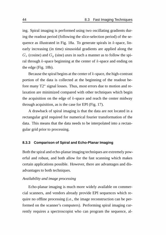
44 8.3 Fast Imaging Techniques
ing. Spiral imaging is performed using two oscillating gradients dur-
ing the readout period (following the slice-selection period) of the se-
quence as illustrated in Fig. 18a. To generate spirals ink-space, lin-
early increasing (in time) sinusoidal gradients are applied along the
Gx (cosine) andGy (sine) axes in such a manner as to follow the spi-
ral throughk-space beginning at the center ofk-space and ending on
the edge (Fig. 18b).
Because the spiral begins at the center ofk-space, the high-contrast
portion of the data is collected at the beginning of the readout be-
fore many T2⋆ signal losses. Thus, most errors due to motion and re-
laxation are minimized compared with other techniques which begin
the acquisition on the edge ofk-space and reach the center midway
through acquisition, as is the case for EPI (Fig. 17).
A drawback of spiral imaging is that the data are not located in a
rectangular grid required for numerical fourier transformation of the
data. This means that the data needs to be interpolated into arectan-
gular grid prior to processing.
8.3.3 Comparison of Spiral and Echo-Planar Imaging
Both the spiral and echo-planar imaging techniques are extremely pow-
erful and robust, and both allow for the fast scanning which makes
certain applications possible. However, there are advantages and dis-
advantages to both techniques.
Availability and image processing
Echo-planar imaging is much more widely available on commer-
cial scanners, and vendors already provide EPI sequences which re-
quire no offline processing (i.e., the image reconstructioncan be per-
formed on the scanner’s computers). Performing spiral imaging cur-
rently requires a spectroscopist who can program the sequence, al-

8 K-SPACE IMAGING 45
though some commercial vendors are beginning to provide some spiral
sequences. Also, because the spiral data are not in rectangular coordi-
nates, offline processing on a remote computer is usually required to
generate images.
Artifacts
EPI suffers from off-resonance problems because there are no refo-
cussing pulses. These off-resonance issues arise from susceptibility ar-
tifacts and fat-water separation and lead to well-recognized distortions
of the images. With EPI any phase errors are propagated throughout
k-space, leading to mismapping and thus distortion on the image. Spi-
ral imaging refocusses periodically in both dimensions leading to less
distorted images. However, the artifacts which occur in spiral images
exist in both dimensions and manifest as blurring of the image rather
than as discrete artifacts as is the case for EPI.
Efficiency
Spiral imaging is slightly more efficient than EPI. In EPI, the x
gradient is not driven very hard, whereas they gradient must be driven
extremely hard (for the socalled ”blips”). Just like any machine or mo-
tor, driving the gradient extremely hard in short bursts requires some
small break for rest. Spiral imaging uses bothx- andy-gradients and
drives both at a high but constant rate. Because there are no sudden
changes in the gradients, less of the break is required. Thisslight
increase in efficiency means that using a spiral trajectory,one can usu-
ally acquire a few more slices than when using EPI at a given temporal
and spatial resolution.

46 8.4 Image Contrast
Small T1
Large T1
Small T1
Large T1
Time
Inte
nsity
Time
DifferenceInte
nsity
1
2
a
b
1
Figure 19: Magnetization/signal recovery after saturation (a) andinversion (b). The times labelled ”1” and ”2” represent the inversiontimes yielding maximum intensity difference between the specieswith small and large T1 relaxation times.

8 K-SPACE IMAGING 47
8.4 Image Contrast
In order to distinguish different types of biological tissue in a magnetic
resonance imaging experiment there must be a contrast or difference in
signal intensity between adjacent tissues. Since the signal intensity is
proportional to the number of spins and thereby with the spindensity
of the voxel, the spin density represents the most pronounced contrast
in the image. However, by using special pulse- and gradient-sequences
it is possible to obtain T1-, T2-, velocity-, or diffusion-weighted im-
ages. How these different contrasts are favoured over oneanother will
be discussed in the following sections.
Prior to presenting these techniques it should be noted thatamong
radiologists and clinicians, the terms T1- and T2 weighted are very
unprecise and typically just refer to experiments using short TR/short
TE (T1-weighted), long TR/long TE (T2-weighted), and finally the
standard (ideal) experiment with long TR/short TE is referred to as
spin-density weighted. A fundamental misconception abouta T1 or
T2 weighted image is that all tissue contrast in the image is dominated
by T1 or T2 effects. Nearly all MR images display contrast primar-
ily related to the proton spin density overlaid by relatively weak ef-
fects from relaxation. The following two sections will discuss how to
achieve the most pronounced contrast between tissues with different
relaxation times.
8.5 T1-Weighted Imaging
Apart from having different proton spin density, the relaxation times
for different tissue also varies. Representative values are listed in Table
2 and do indeed show significant variation from tissue to tissue.
In the ideal case TR should be so large that all signal is recovered
before pulsing the next time, and if TR> T1 there will be at least 99%

48 8.5 T1-Weighted Imaging
Gz
Gx
Gy
Acq
TI180o 90o
rf
Figure 20: Echo-planar imaging pulse sequence equipped with aninitial inversion-recovery block. TI denotes the inversion time (seetext).
Table 2: Representative T1 relaxation times.
Tissuea T1 (ms)0.5 T 1.5 T
Cerebrospinal fluid (F) > 4000 > 4000Skeletal muscle (B/F) 600 870Gray matter (B/F) 656 920Liver (B/F) 323 490Adipose tissue 215 260aB/F denotes bound and free water, respectively.

8 K-SPACE IMAGING 49
of the signal recovered. If TR is shorter, less signal is recovered, which
results in signal loss. However, when tissues with different T1 relax-
ation times are present, we may have relaxation behaviour assketched
in Fig. 19a for two types of tissue with short and long T1 relaxation
times. The two solid curves display how the signals recover as a func-
tion of the repetition time, while the dotted line shows the difference
in signal between the two tissues.
If we want to use the difference in T1 as additional contrast,a sim-
ple experiment to achieve this would be a standard MRI experiment
employing the repetition time labeled ”1” in Fig. 19a. This experi-
ment will partly suppress the tissue with long relaxation time, thus
increasing the image contrast.
To further improve the T1 weighting one may apply the inversion-
recovery pulse sequence shown in Fig. 7 prior to e.g. the echo-planar
imaging sequence as shown in Fig. 20. If the inversion time TIis
adjusted so that the proton magnetization for one of the tissues exactly
crosses zero this tissue will be completely suppressed in the resulting
image as illustrated by the inversion times labelled ”1” and”2” in
Fig. 19b.
It should be emphasized that the inversion-recovery experiment
provides a much better T1 weight than the standard experiments at the
expense of significantly longer experiment time. If both the180◦ and
90◦ rf pulses are slice selective as shown in Fig. 20 it is still possible
to acquire such data using the multi-slice protocol.
8.6 T2- and T2⋆-Weighted Imaging
Just like longitudinal relaxation, transverse relaxation, T2, also varies
from tissue to tissue. Figure 21 depicts the signal decay dueto T2
relaxation for small and large T2 relaxation times. At the echo time
labelled ”1” in this figure, the maximum difference between the two

50 8.7 Creating Contrast Using Contrast Agents
Small T2
Large T2
Time
Inte
nsity
1
Figure 21: Signal intensity as a function of the echo time TE. Thesolid lines represent the signal decay due to small and large T2relaxation times and the dotted line displays the difference betweenthe two solid curves. The echo time labelled ”1” marks the timeyielding maximum difference in the two signals.
signals is achieved.
While the echo-planar imaging sequence (Fig. 17) is dependent
on relaxation under T2⋆ other techniques may refocus the additional
magnetic-field and susceptibility effects discussed in Section 3.2 and
display relaxation behaviour according to T2. A very widelyused se-
quence for achieving this is the fast spin-echo (FSE) sequence shown
in Fig. 22. Rather than using gradient refocussing the magnetiza-
tion, this sequence uses a series of180◦ pulses to create spin echoes.
Thereby the additional T2⋆ effects cancelled.
8.7 Creating Contrast Using Contrast Agents
The beauty of MRI is its ability to create different types of contrast
without injecting any radioactive contrast compounds intothe veins,
as it is necessary for a number of other imaging techniques like PET
and CT. MRI normally relies on the intrinsic contrast between tissues.
However, MRI will also often benefit from using external contrast
agents to increase contrast between different tissues.

9 FUNCTIONAL IMAGING 51
Gz
Gx
Gy
90o 180o
rf
Acq
TE
Figure 22: Fast spin-echo (FSE) pulse sequence. Each echo isobtained using a different phase-encoding step.
MRI contrast agents are indirect agents that will never be visual-
ized directly in the image, but affect the relaxation times of the water
protons in the nearby tissue. Such agents are often paramagnetic and
may be categorized in T1 and T2 relaxation agents depending on their
actual properties.
9 Functional Imaging
The termfunctional imagingmay have several specific meanings. In
all cases the basic idea of functional imaging is, however, to obtain im-
ages displaying physiology rather than simple anatomy. In this Section
we will focus on the most common use of the term functional imag-
ing, abbreviated fMRI. Specifically this technique is used for mapping
brain activation.
Functional imaging relies on the tight coupling between neuronial
activity and blood flow, a coupling that was first proposed in 1890

52
Magnetic susceptibility
Increase
Decrease
T2*
MRI signal intensity
Oxyhemoglobin
Cerebral blood flowOxygen consumption
Brain activity
Deoxyhemoglobin
Figure 23: Mechanism of blood-oxygenation level dependent(BOLD) imaging. Increased brain activity causes increased oxygenconsumption and cerebral blood flow. Hench the oxyhemoglobinlevel increases and the deoxyhemoglobin level decreases. Sincedeoxyhemoglobin is paramagnetic the relaxation time increaseswhen the paramagnetic species is removed, leading to an in-creased MRI signal intensity.

9 FUNCTIONAL IMAGING 53
by Roy and Sherrington. This coupling, although not fully under-
stood, allows for indirect measurement of cerebral activity by monitor-
ing changes in cerebral hemodynamics as illustrated in the flow-chart
in Fig. 23. The T2⋆ relaxation rate of blood changes depending on
whether or not the hemoglobin is bound with oxygen, a phenomenon
first described by Linus Pauling. When the hemoglobin molecule is
bound with oxygen (oxyhemoglobin), blood is slightly diamagnetic.
However, when oxygen is removed from the hemoglobin molecule
(deoxyhemoglobin), it becomes more paramagnetic due to more un-
paired electrons. This increased paramagnetism leads to increased
magnetic susceptibility of the tissue. Changes in magneticsusceptibil-
ity introduces a change in T2⋆ and may be mapped by T2⋆-weighted
pulse sequences like EPI.
Functional imaging takes advantage of the changing signal within
blood and surrounding tissue at the ratio of oxyhemoglobin-deoxy-
hemoglobin changes. When a task or stimulus paradigm is presented
to the person in the MR scanner, the cortical neurons in the area re-
sponsible for processing the information become active. This activ-
ity leads to local increased neuronal metabolism which thenleads to
increased blood flow. However, the increased blood flow is greater
than the metabolic needs of the neurons, thereby resulting in excess
oxygen being supplied to the active area. Thus, the oxyhemoglobin-
deoxyhemoglobin ratio in the capillaries and small veins increases
compared to the situation when the neurons are inactive. This increase
means less deoxyhemoglobin and thus less signal loss from T2⋆ relax-
ation. Thereby an increased signal during the neuronally active state
compared with the resting state is achieved. It is this slight increase
in signal during the active state that is detected in functional imaging.
This contrast methanism is referred to asBOLD (Blood Oxygenation
Level-Dependent) contrast and is the most commonly used MR tech-

54
c d
ba
Figure 24: Three-dimensional, whole brain images of activationduring a language task based on word generation from a phoneme.The test persons were presented phonemes and were asked tothink of as many English words as they could that contained thephoneme until the presentation of the next phoneme. The dark-graypicture is the anatomical image. In light color is the superimposedfunctional map. Brain images shown are (a) left hemispheres (b)right hemispheres, and (c) at an angle where the left hemisphereand top of the brain are both partially seen. In (a)-(c), the anatomi-cal images are opaque; consequently only activated regions that liepredominantly on the cortical surface are seen. Image (d) is iden-tical to (c) except that the anatomical image was rendered partiallytransparent in order to ”look through” and see the activated regionsthat would normally be blocked from the view by overlapping cortex.

10 MAGNETIC-RESONANCE ANGIOGRAPHY 55
nique to evaluate cortical activation.
Since the absolute MR signal differences are very small (< 5%
with 1.5-T systems), appropriate activation mechanisms must be con-
structed, to enable precise measurements of activated and nonactivated
brain states. Since the signal change is due to T2⋆ relaxation, it is mea-
sured by T2⋆-weighted sequences of which echo-planar imaging is the
most widely used.
Figure 24 exemplifies functional imaging. In this Figure, the test
persons were presented phonemes and were asked to think of asmany
English words as they could that contained the phoneme. The images
represent the anatomical image in dark gray overlaid by the functional
map in light colors.
10 Magnetic-Resonance Angiography
Angiography is the imaging of flowing blood in the arteries and veins
of the body. In the past, angiography was only performed by introduc-
ing an X-ray opaque dye into the human body and making an X-ray
image of the distribution of the dye. This procedure createda picture
of the blood vessels in the body. It did not, however, producean im-
age which distinguished between static and flowing blood. Magnetic-
resonance angiography (MRA), on the other hand, produces images
showing theblood flow. The intensity in MRA images is proportional
to the velocity of the flow. In the following two general typesof MRA,
time-of-flight and phase-contrast will be described.
10.1 Time-of-Flight MRA
Time-of-flight angiography can be performed in several ways. One
method uses a spin-echo sequence where the slice-selective90◦ and
180◦ pulses have different frequencies. The90◦ pulse excites spins

56 10.2 Phase-Contrast MRA
in one plane. The180◦ pulse excites spins in another plane. In the
absence of flow, no signal is seen because no spins experienceboth
pulses. However, if the flow matches the slice-distance and TE time,
blood from the90◦ plane flows into the180◦ plane and an echo is
produced. This principle is illustrated in Fig. 25a.
10.2 Phase-Contrast MRA
Phase-contrast angiography is a little more complicated. Recall the
gradient echo which refocusses the magnetization and thus has no net
effect on the spins. However, spins moving in the direction of the
gradient direction will not be refocussed by the gradient echo.
This effect is used to distinguish stationary from moving spins.
In practice, two images are acquired, the first having a gradient echo
(e.g. Gx − G−x), and the second has the echo with reversed sign
(G−x − Gx). Stationary spins will appear identically in the two im-
ages, while moving spins will obtain opposite phases. Thus,the dif-
ference between the two images will only contain signal frommoving
spins while stationary spins disappear.
For illustration, Fig. 25 shows a MRA image of the human head.
This image clearly shows the blood veins in white while the back-
ground signals from stationary tissue are rather weak.
For angiography it may also be beneficial to use contrast agents to
emphasize the blood veins in the images, but it will not be discussed
in more detail here, since the beauty of MRI is its ability to achieve
MRA images using the intrinsic properties of the different tissues.
11 Localized Magnetic Resonance Spectroscopy
In certain cases the images based on the spin density, as discussed so
far, do not provide the desired information. It is often desirable to

11LO
CA
LIZE
DM
AG
NE
TIC
RE
SO
NA
NC
ES
PE
CT
RO
SC
OP
Y57
180o90o
a
b
c
Figure 25: (a) Spin-echo sequence using different frequencies for the 90◦ and 180◦ pulses. This makes themact on different slices. (b) blood vein in which the 90◦ pulse excites only the blood contained in the image slice.During the delay between the pulses this blood flows through the vein. The 180◦ pulse is applied to another slice,and only if the shaded blood volume flows into this slice its magnetization will be refocussed by the 180◦ pulse.(c) Magnetic-resonance angiograph showing the blood arteries in a human head in white and light gray.

58 11.1 Single-Voxel Techniques
monitor the spatial abundance of different metabolites. Signals from
such metabolites appear at different resonance frequencies in an NMR
spectrum and will thus be distinguishable by NMR.
The idea of localized magnetic resonance spectroscopy (MRS) is
to acquire an NMR spectrum for a particular spatial location. Unlike
MRI where voxel sizes of1× 1× 5 mm3 or smaller are available, the
voxel size should typically be larger than1 × 1 × 1 cm3 in MRS to
obtain an acceptable signal to noise ratio.
There are two main techniques for acquiring localized MRS, single-
voxel and multi-voxel techniques.
11.1 Single-Voxel Techniques
Single-voxel techniques acquire spectra from a single small volume el-
ement of the tissue. The most common approaches excite only the de-
sired tissue volume through the intersection of three orthogonal slice-
selection pulses. A pulse sequence that achieves this is shown in
Fig. 26a and is known as point-resolved spectroscopy (PRESS). It uses
a90◦ excitation pulse and two refocussing180◦ pulses, each with dif-
ferent physical gradient as the slice-selection gradient.Only spins lo-
cated in the intersection of all three slices produce the spin echo and
appear in the spectrum. Figure 26c exemplifies applicationsof MRS.
It displays point-resolved spectra of the human brain and inaddition,
two zoomed representative spectra.
11.2 Multi-Voxel Techniques
Multi-voxel techniques are those from which multiple spectra are ob-
tained during a single measurement. The most common of theseis
known as chemical-shift imaging (CSI). CSI techniques are analogous
to standard imaging techniques in that phase encoding gradient tables

11 LOCALIZED MAGNETIC RESONANCE SPECTROSCOPY 59
90o90o 180o 180o 180o
Gx
Gy
Gz
Gx
Gy
Gz
Acq
c
������������������������������������
������������������������������������
������������������������������������
������������������������������������
rfrf
a b
Acq
Figure 26: (a) Point-resolved spectroscopy (PRESS) pulse se-quence timing diagram. (b) Multi-voxel volume selective chemical-shift imaging (CSI) pulse sequence. (c) point-resolved spec-troscopy of the human brain and zoomed representative spectrafrom 1) white matter hyperintensities and 2) normal appearing whitematter.

60
are used for spatial localization. An example of such a sequence is
shown in Fig. 26b.
12 Instrumentation
At the end of these Notes it appears relevant to make a few comments
on the instrumentation used for MRI experiments. Although the MR
scanner is much
12.1 MR Scanners
Figure 27 shows pictures of four different types of scanners. The
whole-body scanner (Fig. 27a) is typically used for scanning of the
body region of the patient. It has the magnetic field aligned along the
body of the patient. The hole in the scanner is typically between 55
and 60 cm, which may limit the size of the patient entering thescan-
ner, but obviously it is much more difficult to manufacture scanners
with larger diameters. The magnetic field strength may be up to 1.5 T
on whole-body scanners.
An important application of MRI is imaging of patients heads.
Thus, specially designed head scanners have been developedas illus-
trated in Fig. 27b. Since the hole in these scanners is much narrower
than in whole-body scanners, the magnetic field strength maybe as
high as 7 T for head scanners.
Finally, it is convenient to have scanners where extremities (arms,
shoulders, legs) may be scanned. Such scanners typically have a much
more open design than the cylindrical head- and whole-body scanners.
For such scanners the magnetic field strength may be up to 3 T.

12IN
ST
RU
ME
NTAT
ION
61
a
dc
b
Figure 27: MR scanners for different purposes. (a) whole-body-, (b) head-, (c,d) extremety-scanners.

62 12.2 Gradient System
12.2 Gradient System
An additional issue that makes MR scanners differ from normal NMR
spectrometers is the need for magnetic field gradients in MR scan-
ners. As mentionned in Section 6 it should be possible to create mag-
netic field gradients in all three dimensions. Figure 28 shows the coil
design used for generation ofz (Fig. 28a) andxy (Fig. 28b) gradi-
ents in whole-body and head scanners. The principle is to place two
electromagnets (coils with high current through them) withopposite
orientation in the direction of the desired gradient. This is relatively
simple for thez gradient which is created by two oppositely oriented
solenoid coils, while thexy gradients are created by sets of socalled
figure-8 saddle coils.
Since the spatial resolution depends on the gradient strength, it
is desirable to have as strong gradients as possible. In practice this
will be a trade off between sensitivity and resolution. Alsothe current
running through the gradient coils may be a severely limiting factor
since too high current through the gradient coils will make them heat
up and eventually quench the magnet. Typically achievable gradient
strengths are on the order of 40 mT/m corresponding to 1.7 MHz/m
for 1H.

12IN
ST
RU
ME
NTAT
ION
63
b
a
Figure 28: Schematic of gradient coils used to generate z (a) and x or y (b) gradients.