Embed Size (px)
Citation preview
MACROINVERTEBRATE COMMUNITY RESPONSES TO CLAM AQUACULTURE PRACTICES I N BRITISH
COLUMBIA, CANADA
Jonathan Arthur Whiteley B.Sc.(Env.), University of Guelph 2001
THESIS SUBMIlTED I N PARTIAL FULFILLMENT OF THE REQUIREMENTS FOR THE DEGREE OF
MASTER OF SCIENCE
I n the Department
of Biological Sciences
@ Jonathan Arthur Whiteley 2005
SIMON FRASER UNIVERSITY
Spring 2005
All rights reserved. This work may not be reproduced in whole or in part, by photocopy
or other means, without permission of the author.
Name:
Degree:
Title of Thesis:
APPROVAL
Jonathan Arthur Whiteley
Master of Science
Macroinvertebrate community responses to clam aquaculture practices in British Columbia, Canada
Examining Committee:
Chair: Dr. A. Harestad, Professor
Dr. L. Bendell-Young, Professor Department of Biological Sciences, S .F.U.
Dr. A. Mooers, Assistant Professor Department of Biological Sciences, S.F.U.
Dr. R. Ydenberg, Professor Department of Biological Sciences, S .F.U
Dr. A. deBruyn, Adjunct Professor School of Resource and Environmental Management, S.F.U. Public Examiner
rr* l I S i b c Date Approved
. . 11

SIMON FRASER UNIVERSITY
PARTIAL COPYRIGHT LICENCE The author, whose copyright is declared on the title page of t h s work, has granted to Simon Fraser University the right to lend this thesis, project or extended essay to users of the Simon Fraser University Library, and to make partial or single copies only for such users or in response to a request from the library of any other university, or other educational institution, on its own behalf or for one of its users.
The author has further granted permission to Simon Fraser University to keep or make a digital copy for use in its circulating collection.
The author has further agreed that permission for multiple copying of t h s work for scholarly purposes may be granted by either the author or the Dean of Graduate Studies.
It is understood that copying or publication of this work for financial gain shall not be allowed without the author's written permission.\
Permission for public performance, or limited permission for private scholarly use, of any multimedia materials forming part of t h s work, may have been granted by the author. This information may be found on the separately catalogued multimedia material and in the signed Partial Copyright Licence.
The original Partial Copyright Licence attesting to these terms, and signed by this author, may be found in the original bound copy of this work, retained in the Simon Fraser University Archive.
W. A. C. Bennett Library Simon Fraser University
Burnaby, BC, Canada
ABSTRACT
Despite recent growth of shellfish aquaculture in B.C., Canada, very little
is known regarding impacts of common practices. Seeding and netting are
frequently employed on clam farms to increase production of' Venerupis
philippinarum. A pilot netting experiment found no observable effect of
predation at small scales. A field study compared bivalve communities on clam
farms with matched reference sites, using density and biomass data. V,
philippinarum was the only species found in higher abundance on farm sites,
consistent with values expected from clam seeding. Bivalve communities were
not significantly different on farm sites, but were more similar on average than
reference sites, leading to a loss of regional distinctness. These results are
consistent with recent research suggesting that predation and competition may
play minor roles in structuring communities in soft-bottom environments. Given
the remaining uncertainties, a precautionary approach is recommended in future
development of the intertidal for clam aquaculture.
iii

I am forever grateful to Leah Bendell-Young, for supervising and funding
this project, and to all members of my supervisory committee, Ron Ydenberg and
Arne Mooers, for asking the hard questions and for their invaluable advice. I
wish to thank Judy Higham and Deb Lacroix for help with planning, paperwork
and other administrative necessities. I can't thank Molly Kirk enough for her
hard work and dedication as a field technician, and Ian McKeachie, Kate
Henderson, David Leung, Natalie Martens, Vanessa Sadler, Robyn Davidson,
Blake Bartzen, Rian Dickson, and Tyler Lewis, who also sifted through beach
sediment and collected samples in adverse weather to collect data for this
project. I thank Dan Esler, Rob Butler, Sean Boyd, and Tyler Lewis for
collaborating on the Sustainable Shellfish Aquaculture Initiative and for sharing
their thoughts, feedback and results with me.
This work would not have been possible without the co-operation of the
clam farmers who granted permission to sample on their leases and I am
thankful for all their support. I would also like to thank Sarah Dudas, Bamfield
folk, Rick Harbo and others who helped with identification of unknown critters.
Thanks also to Ramunas Zydelis for introducing me to PRIMER software and
multivariate community analysis, and to Colin Bates for helping me understand it.
I am also grateful to Ian Bercowitz, of the Statistical consulting service at S.F.U.,
who answered many questions about repeated measures analysis and other
statistical procedures. Many thanks to Joline Widmeyer, Christy Morrissey, Niki
Cook, Tracey Brunjes, Carolyn Duckham, Jeff Christie, and all the lab-mates and
fellow grad students who listened to my frustrations, successes, advice, and
shared theirs with me.

Approval ......................................................................................................... ii ...
Abstract ............................................................................................................... III Dedication ........................................................................................................... iv
Acknowledgements .............................................................................................. v
Table of Contents ................................................................................................ vi ...
List of Figures .................................................................................................... VIII
List of Tables ....................................................................................................... x ..
Definition of Terms ............................................................................................ xu
Introduction ............................................................................................ 1 Clam Aquaculture in British Columbia. Canada ............................................... 2 Clam Netting .............................................................................................. 4 Predator Exclusion: Current Theory and Evidence ........................................... 6
Building on research in Rocky Intertidal Habitats ........................................ 7 Predation in soft-bottom marine benthic communities ................................. 9 Infaunal Predation & Predator Exclusion Netting ........................................ 14 Competition in soft-bottom marine benthic communities ............................ 16
.................................................. Measuring differences in non-target species 19
Materials and Methods .......................................................................... 21 ................................................................................................ Study Area 21 .............................................................................................. Field study 24
........................................................................................... Study Sites 24 Sampling methodology ........................................................................... 28 Statistical Treatment and Analysis ............................................................ 30
.................................................................................... Netting Experiment 36 Study Sites and Treatment Structure ........................................................ 36
........................... ........................*............ Sampling methodology .. .. .. 38 Statistical Treatment and Analysis ............................................................ 38
Results .................................................................................................. 42 Field Study - Infaunal Bivalve Community ..................................................... 42
....................................................................................... Pre-Farm Sites 42 Density and Biomass .............................................................................. 45 Univariate Community Indices ................................................................. 48
............................................................................... Multivariate Analysis 50 .................................................................................... Netting Experiment 60
................................................................................................ Density -60
................................................................. Univariate Community Indices 62 ............................................................................... Multivariate Analysis 64
Discussion ............................................................................................. 68 .................................................................... Netting and Predator Exclusion 69
.......................................................... Why only Venerupis philippinarum? 70 ................................................ No Observed Effects of Predator Exclusion 72
................................................................................... Which Predators? 75 ............................................................. Where have all the clams gone? 76
.............................................................................................. Zonation -77 ......................................... Physical Changes of Predator Exclusion Structures 80
................................................................................ Change and Variability 81 ............................................................ .......................... Scale of changes '. -85
Summary and Conclusions .................................................................... 90
Appendix A: Sediment Classification ................................................................ 93
Appendix B: Effect of Sieve Mesh Size .............................................................. 94 ................................................................................................ Methods & Analysis -95
............................................................................................ Results and Discussion 97 Conclusion ........................................................................................................... 102
Appendix C: Data Matrixes .............................................................................. 103
Appendix D: Species Lists ............................................................................. 114 Field Study (Infaunal Bivalves) ............................................................................... 114 Netting Experiment (Macrofauna) ........................................................................... 115
References ....................................................................................................... 117
vii
Figure 1. British Columbia (B.C.) Canada. Location of three study areas highlighted with stars. Within each region, study sites are labelled with circles (open for reference sites, closed for farm sites). Outline map adapted from Natural Resources Canada, with permission (http://atlas.gc.ca). ............................................................................... -23
Figure 2. Location of Sites used in Netting Experiment, within Baynes Sound, B.C ....................................................................................................... 37
Figure 3. Mean clam density (individuals-m-2) at field study sites. Shaded bars indicate densities of Venerupis philippinarum, open bars layered behind indicate total clam density. Circles indicate density of all clams, excluding V, philippinarum (shaded = farm site, open = reference site). Error bars represent 95% confidence intervals about
................................................................................ each mean.
Figure 4. Mean clam biomass (g.m'2) at field study sites. See Figure 3 caption for explanation of symbols. ..................................................................... 46
Figure 5 (a & b). MDS Plot of average density (individuals-m-2) of clam species (a, stress = 0.18) and results of the same analysis, with Venerupis philippinarum excluded (b, stress = 0.19). Sites are identified by region (+ = Barkley sound, = Baynes Sound, = Desolation Sound), stratum (black = low, grey = mid), and type (open = reference, closed = farm). Site labels ending in a dash (D3-, A5-) indicate "pre-farming" sites. Active farm sites have also been outlined in a dashed line within the reduced ordination space. ...................
Figure 6 (a & b). MDS Plot of average biomass (g-m-2) of clam species (a, stress = 0.22) and the results of the same analysis, with Venerupis philippinarum excluded (b, stress = 0.23). See Figure 5 caption for labels and legend. ................................................................................ ..52
Figure 7. Mean pairwise Bray-Curtis Similarity (of fourth-root transformed data) within groups. Values for farm sites are on the left of each pair, shaded in grey. White bars represent values for reference sites. Error bars show 95% confidence intervals about each mean. ...................... 54
viii
Figure 8. Mean Density (~nividuals-m-2) of fauna at each plot for time 0, 1 and 2. Values for netted plots are shown in black circles connected by a black line. Control means are plotted in open circles connected by a grey line. Error bars represent individual 9S0/0 confidence intervals for treatment means of plot values. .............................................. ... .... 61
Figure 9. MDS ordinations of plots at each sampling time (t = 0, 1, 2). Plots are identified by location (W = Hint, = Bub, + = Roy), stratum (grey = A, black = B), and treatment (closed = netted, open = control). Stress values are 0.05 (t=O), 0.06 (t=l), 0.04 (t=2). ................... 65
Figure 10. Combined MDS ordination of all plots and sampling times. See Figure 9 caption for explanation of symbols. Samples from the same plot are joined by lines, and labelled by sampling time (0,1,2). Stress =
Figure 11. Macrofaunal density (individuals-m-2), species richness per sample (quadrat) and per site for large and small sieve samples. Results from the small sieve (1 mm mesh) are plotted on the left side, in grey, with results from the large sieve (6 mm mesh) on the right, in white. Values represent means across all sites with 95% confidence intervals (error bars). ............................................................................. 97
Figure 12. Number of species observed at a site as a function of the number of individuals in the pooled sample. Values from the large sieve (6 mm mesh) are plotted as X's and values from the small sieve (1 mm mesh) as dots. The lines are logistic regressions of #spp on In(#individuals): large in black, small in grey. ........................................... 98
Figure 13. Shared species between large and small sieves in pooled sample (over all sites) and averaged per site. Number of species shown as values in each bar. ................... .... ..................................................... 99
Figure 14. Number of individuals per species in the large versus small sieves (67 shared species only). Values are averaged over all sites, converted to #individua~s.m-~, and plotted on a log-log scale to scatter points and include the large range of values. .................................................... 100
Table 1.
Table 2.
Table 3.
Table 4.
Table 5.
Table 6.
Table 7.
Table 8.
Table 9.
Characteristics of study sites, including sample size (# quadrats sampled). Sites are labelled by region (A = Baynes Sound, B = Barkley Sound, D = Okeover Inlet, Desolation Sound) and a number, to identify each pair. * Indicates sites that were seeded without nets ..................................................................................................... .25
Bivalve density, biomass, and community indices for pre-farm sites. ............ 44
Results of weighted paired analyses of bivalve abundance, including Mean Difference (Farm-Reference) *95% confidence interval width (with degrees of freedom), for each estimate. Mean differences significantly different from zero (2-tailed) are highlighted in bold, with *. Site D2, in the mid stratum, was highly influential in tests using biomass data and a potential outlier, so was omitted from the calculation ........................................................................................... -47
Number of observed and estimated clam species, values of diversity and evenness indices at each site. ........................................................... 49
Results of paired analysis and tests for equality of variances (F- test) for estimates of species richness, evenness and diversity, between farm and reference sites. Significant differences (a = 0.05) are highlighted in bold with * ........................................................................ 49
ANOSIM results for bivalve community. Factors in 2-way crossed analyses are listed with the crossed factor identified in brackets. Statistically significant results are highlighted in bold with an asterisk *. ......................................................................................................... 53
Consistency of species' contributions to the similarities within farm and reference sites, by density. Species are listed in the order of their contribution to the average similarity within the group ........................ 55
Species responsible for 90% of the dissimilarity between farm and reference sites, listed in order of importance of their contribution to the average Bray-Curtis dissimilarity. Density values listed are untransformed average density (individuals-m-2) in each group. ................. .57
Species responsible for 90% of the dissimilarity between farm and reference, listed in order of importance of their contribution to the average Bray-Curtis dissimilarity. Biomass values listed are untransformed average biomass (g.m-2) in each group ............................... 59
Table 10.
Table 11.
Table 12.
Table 13.
Table 14.
Table 15.
Table 16.
Table 17.
Table 18.
Table 19.
Results of repeated measures analysis for paired group densities (individ~als.m'~, Net - Control plot). Significant p-values (a=0.05)
are highlighted in bold with an asterisk * .................. ....... ................ 62
Observed, estimated species richness, diversity and evenness for all netting experiment plots. ........................................................................ 63
Results of repeated measures analysis of paired differences (Net - Control plot) for estimated species richness, evenness and diversity. Significant p-values (a=0.05) are highlighted in bold with an asterisk
ANOSIM results of factor comparisons at each sampling time. Small sample sizes only permitted 100 randomizations for each test ..................... 66
ANOSIM results of comparisons between sampling times, within .......................................................................................... treatments. .67
ANOSIM results of factor comparisons across all sampling times. Significant differences (a=0.05) are highlighted in bold with an
............................................................................................. asterisk *. 67
Densities of species more abundant in small sieve (1 mm mesh) than the large. ......................................................................................... 101
Density data matrix (mean # individuals-m'2) for field study (Bivalve community). ........................................................................................ 105
Biomass data matrix (mean g-m'2) for field study (Bivalve community). ........................................................................................ 107
Data matrix (pooled counts over 5 quadrats) for netting experiment.. ....... . I 0 9
Intertidal:
Mid Intertidal:
Low Intertidal:
Soft- bottom:
Rocky Bottom:
Infauna:
Epifauna / Epibenthic:
The area of land normally exposed and covered during an average tidal cycle. This is typically defined as extending from the yearly average of the lowest low tide level to the average of the highest high tides among each cycle.
I n this work, "Mid" intertidal refers to beach areas between 2m and 3m above chart datum.
I n this work, "Low" Intertidal refers to beach areas between l m and 2m above chart datum.
Benthic substrate composed primarily of unconsolidated clastic sediment particles, typically deposited by water movement. This includes a range of substrate types, from mud to loose cobble. Appendix A defines substrate types in terms of particle sizes.
Benthic substrate composed primarily of solid mineral structures, such as cliff faces and bedrock.
Refers to animals that are typically found below the sediment surface, in soft-bottom benthic environments.
Refers to animals that are typically found on the surface of benthic environments.
xii

The role of biodiversity in ecosystems has become a major concern of
scientists and the public, in light of increasing numbers of documented species
extinctions. If biodiversity is to be maintained, a greater understanding is
required of the mechanisms that structure this diversity, and ecologists are
particularly interested in the diversity of species and the structure of their
associated communities. Ecological factors that are important in structuring
diversity at a local scale include predation, competition, migration, physical
structures, environmental and habitat complexity, and disturbance. The relative
importance of these factors may vary between ecosystems and each can operate
individually or in combination to structure local diversity.
The research described in this work is intended to assess in a descriptive
manner if and how practices associated with shellfish aquaculture of clams in
British-Columbia (B.C.), Canada are associated with changes in species diversity
or community structure of intertidal benthic macroinvertebrate communities.
The goal is to quantify the potential impacts of an expanding shellfish
aquaculture industry over large regional scales in coastal B.C.
Because predator exclusion is an important aspect of clam aquaculture in
B.C., this industry offers a unique opportunity to examine the roles of predation
and competition in structuring intertidal communities. Results from field studies
and a small experiment will be used to explore differences in the community
structure of macroinvertebrates associated with common shellfish aquaculture
practices, in soft-bottom intertidal habitats.
I. I Clam Aquaculture in British Columbia, Canada
Bivalves are an important component of many soft-bottom marine
communities. Their activities play a major role in cycling nutrients between
sediments and the overlying water column (Dame 1996). Filter and deposit-
feeding by many bivalves aid in moving nutrients and organic particles from the
water column into sediments. Bivalves also excrete metabolic biproducts back
up into the water. The burrowing activities of bivalves and other infaunal
invertebrates also mobilize nutrients stored in the sediments back up into the
water column, a process known as bioturbation (Groffman and Bohlen 1999,
Snelgrove 1999). Infaunal bivalves (clams) also serve as an important food
source for a variety of marine predators, including crabs (Spencer et a/. 1992),
worms (Bourque et al. 2001), fish (de Goeij et a/. 2001), snails (Peitso et a/.
1994), birds such as sea ducks (Jamieson et a/. 2001) and humans.
Clams were harvested traditionally by aboriginal people in British Columbia
(B.C.), Canada prior to European settlement, and there has been a clam fishery
in B.C. since the late lgth century (Quayle and Bourne 1972). The industry
initially consisted of commercial harvesting, predominantly of butter clams
(Saxidomus gigantea; Des hayes 1839) and native littlenecks (Protothaca
staminea; Conrad 1837). Japanese littlenecks, or manila clams ( Venerupis
philippinarum; A. Adams & Reeve, 1850) were introduced to B.C. with Japanese
oyster seed (Crassostrea gigas; Thunberg, 1793), and first recorded in 1936
(Quayle and Bourne 1972). After spreading throughout southern areas of
coastal B.C., they have grown in importance to become the single largest
component of the clam fishery and clam aquaculture in the region (Harbo 1997).
Other clam species have been introduced to B.C., including a deliberate
release of Mya arenaria, a commercially valuable species on it's native Atlantic
shores that has never achieved a similar popularity in B.C. (Quayle and Bourne
1972). A more recent invasion by the varnish clam, also known as the dark-
mahogany or savoury clam (Nuttallia obscurata; Reeve, 1857) occurred in the
late 1980s to early 1990s (Harbo 1997). Nuttallia obscurata is generally thought
to have arrived from Japan in ballast water (Gillespie etal. 1999). This new
arrival has primarily colonized intertidal areas even higher than Venerupis
philippinarum, which might allow it to avoid competition with other intertidal
clam species, or intense predation prevalent in lower intertidal areas.
Aquaculture of clams in B.C. began in an experimental stage in Baynes
Sound (see Figure 1) in 1969, but has only been licensed formally since 1991
(Jamieson etal. 2001). Access to suitable sites has been identified as a major
factor limiting the expansion of shellfish aquaculture (Coopers & Lybrand 1997),
and the industry has turned to increasing the intensity of production at existing
sites (BCSGA 2004a). Venerupis philippinarum is the commercially dominant
species in the industry. Production of this species is enhanced on tenures
primarily using a combination of two common practices: (1) the addition of
hatchery-reared juvenile Venerupis philippinarum to intertidal sediments, a
process referred to as "seeding", (2) the application of netting over the seeded
substrate to protect the juvenile clams from predation (Jamieson etal. 2001).
Clams are harvested year-round using hand-raking, once they reach a minimum
legal size of 38 mm (1.5 inches) approximately 2-4 years after seeding (Jamieson
et al. 2001).
I .2 Clam Netting
Protective nets used in B.C. include a variety of plastic netting with 1.25
cm apertures, called 'car cover" by many farmers, and woven rope netting with
apertures up to approximately 3.5 cm. These nets are applied in 1 or 2 layers,
then anchored at the corners and along the edges with large rocks, or steel
posts, bent into an inverted U-shape and pounded into the sediment. Similar to
observations by Spencer et a/. (1996, 1997), nets used in B.C. frequently attract
growth of macroalgae and other "bio-fouling" organisms, which must be
removed manually as large amounts can reduce the availability of food particles
to the sediment surface (Jamieson etal. 2001). In some areas, the amount of
labour required to keep nets clear of biofouling is so great that some clam
farmers have abandoned the use of nets in intertidal areas (personal
communication).
There appears to be no consensus among clam farmers regarding the
reasons for applying nets over cultured clam beds. This practice was originally
proposed to protect the clams from predators in the water column (Spencer et
a/. 1992). While survival of juvenile Venerupis philippinarum is enhanced by
netting (Spencer etal. 1992), survival of larger individuals of this species
appears unaffected by netting (Jamieson et a/. 2001). Spencer et a/. (1997)
reported a survival rate of only 5% for adults under netted plots, and farmers
expect a 40-50% loss of their crop even under nets (BCSGA 2004b).
Some believe that the stabilizing effect on the sediment is more important
than protection from predators. Nets tend to increase sedimentation rates in
intertidal areas, with a subsequent benefit to bivalves through an increase in the
availability of food particles (Spencer etal. 1996). Increased sedimentation can
also lead to changes in community structure, independent of predator exclusion.
This sampling artefact has been a common confounding factor in many predator-
exclusion experiments that use structures such as nets or cages to exclude
predators from soft-bottom marine sediments (Gee et al. 1985, Reise 1985).
I n the UK, netting cover for cultured clam beds was also proposed to
prevent the introduced cultured clam species, Venerupis philippinarum, from
escaping and colonizing local habitats (Spencer etal. 1996). I n order to achieve
this, the netting was buried along all edges, to an unspecified depth. Although
the same Japanese species, V. philippinarum, is cultured in B.C., netting is not
applied in a comparable manner. This species is capable of breeding in southern
B.C. coastal waters and was already well established in the wild before clam
aquaculture and netting was present in the region. Offspring from cultured
clams colonize areas outside shellfish tenures, where they are harvested along
with wild set by recreational users with a fishing license, wild harvesters with a
commercial license, and poachers, who are the largest unknown and unregulated
harvesters.
1.3 Predator Exclusion: Current Theory and Evidence
Whether intentional or not, the presence of netting in soft-bottom
intertidal habitats is likely to exclude large, epibenthic predators from access to
infaunal prey species. The exclusion of predators is often used as an
experimental, though indirect means of manipulating the intensity of
competition. The removal of intense predation pressure theoretically allows
populations to reach a carrying capacity where resources become limiting, and
the effects of competition should be observed. Experimental evidence, however,
has shown inconsistent effects of excluding predators from marine benthic
environments.
1.3.1 Building on research in Rocky Intertidal Habitats
Caging experiments have demonstrated that predators help to maintain
species richness and diversity in rocky bottom communities (Dayton 1971, Gee et
a/. 1985, Paine 1974). When large, mobile predators are excluded with cages,
populations of producers and sessile organisms increase to a point where space
on the surface on the rocky habitat becomes limiting, and interspecific
competition becomes more important in structuring communities. Species that
lose out in competition are excluded from these areas, and all available space
becomes occupied by a few, dominant species (Dayton 1971).
These observations suggest that predation keeps populations of
competitively superior species low enough to create empty patches on rocky
substrata, which are available to be colonized by other opportunistic species.
Predation is thought to reduce the dominance of otherwise competitively superior
species, effectively depressing the strength of interspecific competition (Paine
1974).
Many broad ecological theories about the structuring role of competition in
communities have been based on results from experiments in rocky- bottom

habitats (Peterson 1992). This may be a result, in part, of the relative ease of
conducting experiments in these systems. The challenges of sub-surface,
sediment-dwelling organisms that are difficult to capture or observe in their
natural setting, along with the complexity of interactions in benthic food webs
may have discouraged early experimentation in soft-bottom systems. However,
Peterson (1992) argues that organisms in these habitats are less mobile than
other (terrestrial) environments, but easily transportable as they are not directly
attached to the substrate. These characteristics make this system extremely
amenable to "rigorous experimental manipulation", once the challenges of
finding and counting such fragile organisms are overcome.
Recent research in soft-bottom benthic systems suggests that space is not
as limiting a factor as it is in rocky-bottom habitats, due to the three-dimensional
nature of sediments, and the relatively greater mobility of organisms (Peterson
1979b, 1992). This increased habitat complexity may offer more opportunities
for competition avoidance, even in the absence of predation. Therefore,
competition may not play an important role in structuring benthic marine
communities in soft-bottom sedimentary habitats. As a result, the exclusion of
predators does not often lead to changes in community structure in soft-bottom
substrata, because interspecific competition may not be enhanced in the absence
of predators. This contrasts sharply with results from experiments in rocky
bottom environments, due to fundamental differences in physical and biotic
characteristics between these two ecosystems. Any theory regarding the
structuring role of predation in soft-bottom habitats can not be inferred from
research conducted in rocky bottom environments, but must be based on direct
observations from soft-bottom communities themselves.
1.3.2 Predation in soft-bottom marine benthic communities
Predator exclusion experiments and studies in soft-bottom habitats have
found at times strong or weak effects of predation on community structure.
Current theory predicts that predation could play an important role in structuring
communities if it is intense enough to limit populations below the point at which
competition, or some other factor becomes more important and structures
communities differently. I f predation is not limiting when present, it would be
unlikely to affect community structure.
Although experiments often disagree on the mechanisms or role of
predation in structuring soft-bottom benthic communities, the evidence strongly
suggests that predation is often limiting for many benthic populations in
unvegetated sediments (Peterson 1979a, 1982, 1983, Quammen 1984, Reise
1985, Summerson and Peterson 1984). Several experiments have found that
when predators are excluded from these systems using various forms of cages
and nets, that overall densities within exclosures tend to increase, sometimes
double or more that of controls (Reise 1985). Summerson and Peterson (1984)
found that the response to predator exclusion varied by physical and trophic
position within unvegetated sediment. Suspension feeders benefited the most,
followed by predator-scavengers, while surface and sub-surface deposit feeders
responded very little, and deep-dwelling deposit feeders responded the least.
These differences were explained by relative susceptibility to predation. Deep-
dwelling species are naturally well protected from large, mobile predators on the
surface. Many deposit feeders are prey, not only to epibenthic predators, but
also infaunal predator-scavengers such as polychaete and nemertean worms.
These predator-scavengers, in turn, are often the largest of the benthic
macroinvertebrates, least costly to consume, and therefore make excellent prey
for epibenthic predators. Suspension feeders, who must expose some part of
their body to the water column to obtain food, seem to be the most susceptible
to predators on the surface and in the water. Posey et a/. (2002) found similar
increases in the density of sedentary and near-surface dwelling fauna when
predators where excluded.
Such differential responses to predation might lead to a prediction of
changing community structure in exclosure plots, although Summerson and
Peterson (1984) also reported no changes in species richness (number of species
present), evenness (dominance), or diversity (heterogeneity). Any such
differences could be explained by a simple, additive curve of species
accumulation with increasing number of individuals sampled. Thus, as
abundances of benthic species increased, so too did their chance of being
observed in a sample, in a simple additive fashion. The total number of species
present likely did not change.
I n a study of a predatory moonsnail, Polinices duplicatus, Wiltse et a/.
(1980) found a significant negative relationship between predator density and
the number of observed species, evenness, diversity, and density of benthic
invertebrates. This negative effect of predation was attributed to the high
specificity of the predator, which selectively preyed on thin-shelled bivalves and
other rare species in the community, having little or no impact on already
dominant species. The use of observed species as a metric of richness may not
allow a sound conclusion that species were actually excluded by predators,
because if densities of rare species are depressed so as to reduce the probability
of detection in a sample, they would not be observed, despite being present at
extremely low densities. A non-parametric estimator of richness is often
preferred over observed richness and might be more appropriate in this situation
(Brose etal. 2003, Foggo etal. 2003, Gray 2002, Hellmann and Fowler 1999,
Heltshe and Forrester 1983). Nevertheless, the depression of rare species
leading to increased dominance by already dominant species, definitely accounts
for lower evenness associated with this predator. This predatory moonsnail was
also found to have negative effects associated with its burrowing activities,
independent of feeding impacts. Sediment disturbance caused by burrowing and
foraging movements within the sediment were also found to decrease densities
of certain species (Wiltse 1980). It was concluded that this predator was able to
maintain "population densities below the level where strong competition would
occur" (Wiltse 1980).
Disturbance by predation, or any number of other environmental sources,
may also negatively affect bivalves or other benthic invertebrates. Beal et a/.
(2001) found a slight increase in growth rates of bivalves in predator exclosures
in low intertidal areas, but not in mid or high intertidal. It was hypothesized that
this increase may have been due to reduced disturbance by predation, which
incurs metabolic costs of repositioning oneself within disturbed sediment, or of
activities related to predator avoidance (see Beal eta/. 2001). Thus, even if
densities of larger benthic invertebrates are not increased in the absence of
predation, total biomass might increase instead as a result of higher growth
rates.
Many long-term experiments have found seasonal changes in the effects
of epibenthic predators. I n most cases, a release from the limitation of
epibenthic predation was strongest during late summer, and warmer water
temperatures, when larger predators (excluded by 6 mm wire mesh) were most
metabolically active (Drake and Arias 1996, Quammen 1984, Reise 1985). At
other times of the year, benthic populations may presumably be limited by other
sources of mortality (Gee et a/. 1985) such as metabolic constraints, stress and
disturbance, or possibly food.
Impacts of predation can also be size-specific. Bivalves may face
predation from different sources at different stages of their life-cycle (Peterson
1982). Planktonic larvae are most susceptible to predation by planktonic
predators and suspension filter-feeders, including adults of their own species,
until settlement in a benthic habitat, where they may still be prey to deposit-
feeders on and within the sediment. Once juveniles are large enough, predators
may be able to choose individuals based on energetic payoffs, and predation is
expected to be most intense from fish, shorebirds, and small crabs, which often
remove the entire shell and body, leaving no evidence of the prey. Larger adult
bivalves may reach a 'size refuge" and become too large for these predators to
handle, although larger individuals may face an increase risk of predation from
even larger predators, such as shell-boring gastropods, large crabs (Peterson
1982), and humans.
Impacts of predation on community structure generally depend on which
predators have access to a particular community, and how the physical structure
of that community mediates the efficiency of the predators. Experimental
evidence in unvegetated soft-bottom marine habitats generally supports the
hypothesis that predation is often limiting in these environments. It may occur
seasonally, or continuously, or affect some components of the community
selectively. Nevertheless, large epibenthic predators are able to keep
populations of benthic infaunal invertebrates below carrying capacity. When
such predators are excluded from soft-bottom intertidal systems, some, if not all
portions of the community are expected to increase in density or biomass in the
absence of all other limiting factors such as disturbance, competition, food or
other resources.
This is particularly relevant in B.C., where exclusion nets that were
originally developed in the United Kingdom to exclude crabs (Spencer etal.
1992) are now being applied to also exclude scoters, fish and other large
predators. The British Columbia Shellfish Growers' Association (BCSGA) asserts
that without such predator exclusion, approximately 40% of clams would be lost
to predation, in addition to the 40-50% expected losses even under such nets.
Relative strengths of predation may be variable within B.C., although fish, crabs,
and a variety of shorebirds and diving ducks are abundant in many areas of
coastal British-Columbia, often in areas that may coincide with shellfish
aquaculture tenures (Jamieson et a/. 2001). These species are each important
epi benthic predators of soft-bottom communities and are potentially excluded by
clam netting.
1.3.3 lnfaunal Predation & Predator Exclusion Netting
Ambrose (1984) reminds us that not all predators of soft-bottom
communities are epibenthic, and that several species of infauna (polychaetes,
nemerteans, gastropods) are themselves also predators of other infauna.
Infaunal predators are not excluded by nets, cages or other physical structures
often used in predator exclusion experiments carried out in soft-bottom systems.
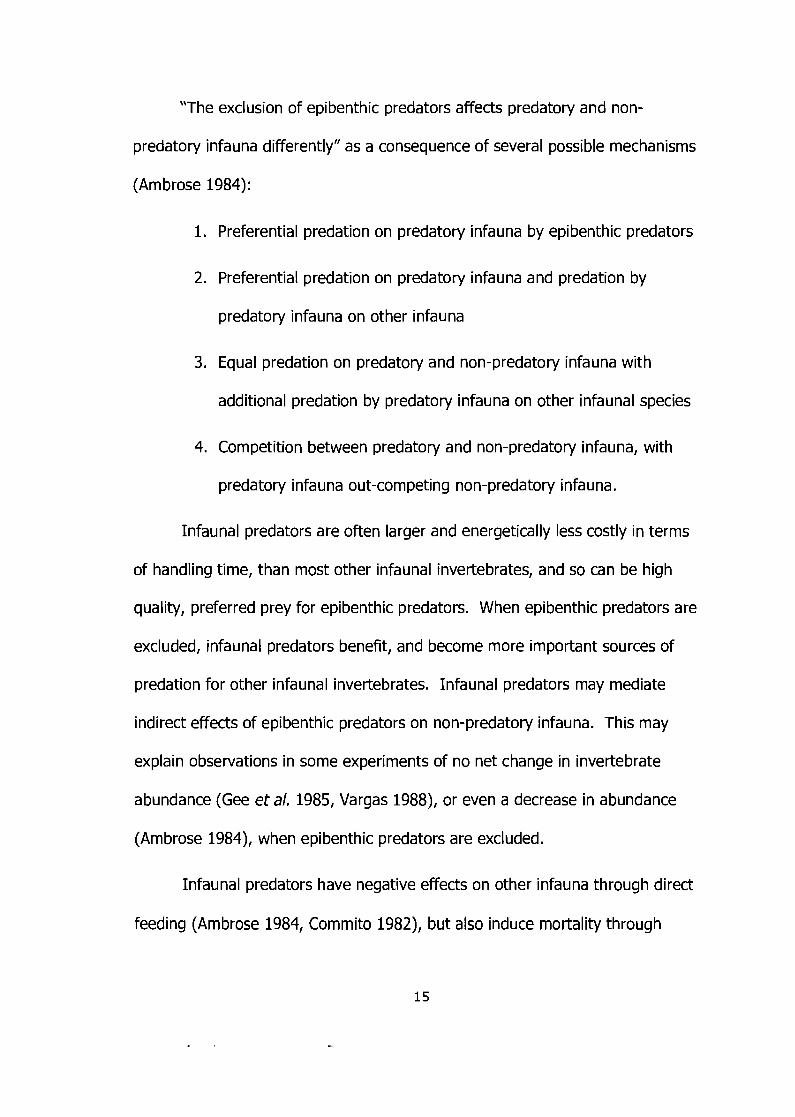
"The exclusion of epibenthic predators affects predatory and non-
predatory infauna differently" as a consequence of several possible mechanisms
(Am brose 1984) :
1. Preferential predation on predatory infauna by epibenthic predators
2. Preferential predation on predatory infauna and predation by
predatory infauna on other infauna
3. Equal predation on predatory and non-predatory infauna with
additional predation by predatory infauna on other infaunal species
4. Competition between predatory and non-predatory infauna, with
predatory infauna out-competing non-predatory infauna.
Infaunal predators are often larger and energetically less costly in terms
of handling time, than most other infaunal invertebrates, and so can be high
quality, preferred prey for epibenthic predators. When epibenthic predators are
excluded, infaunal predators benefit, and become more important sources of
predation for other infaunal invertebrates. Infaunal predators may mediate
indirect effects of epibenthic predators on non-predatory infauna. This may
explain observations in some experiments of no net change in invertebrate
abundance (Gee et a/. 1985, Vargas 1988), or even a decrease in abundance
(Ambrose 1984), when epibenthic predators are excluded.
Infaunal predators have negative effects on other infauna through direct
feeding (Ambrose 1984, Commito 1982), but also induce mortality through
physical disturbance and alteration of surface sediment caused by these large
predators ploughing through the sediment as they move. Such disturbance
effects may be difficult to separate from predation effects (Ambrose 1991).
Ambrose (1991) notes that "infaunal predators may have their greatest effects
on prey population dynamics as a consequence of injuring their prey rather than
consuming it". Infauna have also been observed to emigrate from the sediment
in response to predators. Experimentally observed reductions in infaunal
densities can therefore be a result of emigration rather than mortality.
Infaunal predators certainly have the ability to limit infaunal prey
populations and may often be important in determining community structure, but
mechanisms, and generality of results, to different predatory species and
habitats, has "barely been investigated" (Am brose 199 1). Nevertheless,
conclusions from studies of epibenthic predator exclusion may be dramatically
different if predatory infauna are not considered separately from other infauna.
After all, "predatory infauna are predicted to have their largest effects in habitats
where other forms of control (abiotic disturbance and epibenthic predators) are
rare or of reduced importance" (Ambrose 1991) such as under clam netting.
1.3.4 Competition in soft-bottom marine benthic communities
I n some systems, the primary role of predation in structuring communities
is to limit populations below a point where intense competition would result in a
different community structure. Epibenthic predators have the ability to limit
populations of infaunal macroinvertebrates, predatory and otherwise, below
carrying capacity. The question remains whether competition becomes an
important structuring force in soft-bottom systems, particularly in the absence of
epibenthic predation.
Competition for space has been documented for a few species of large,
deep-dwelling bivalves (Peterson and Andre 1980), although such competition
has not been observed to result in mortality, only reduced growth. Competition
for space can also be avoided by burial at different depths (Peterson and Andre
1980). Certain pairs of species, such as burrowing shrimp and clams, tube
worms and shrimp, are able to alternately dominate soft-bottom communities by
modifying the sediment to mutually exclude each other (Peterson 1984). Black
and Peterson (1988) describe these as cases of "indirect interference operating
through environmental alterations", and not true interspecific competition.
Based on more recent experiments of density-manipulation, in combination with
predator exclusion, it was later concluded that "competition is largely ineffective
in structuring communities of benthic infauna in soft substrata" (Black and
Peterson 1988).
On the other hand, intraspecific competition may increase in the absence
of predation, and food is often proposed as the limiting resource (Gee etal.
1985, Peterson 1982, 1983, 1992, Peterson and Beal 1989, Reise 1985,
Summerson and Peterson 1984). Density-dependent growth has been observed
in several cases, with growth rate and also reproductive output simultaneously
decreasing with increasing density, despite large amounts of apparent space
available, suggesting food depletion to be responsible (Peterson 1982, Peterson
and Beal 1989). I n cases of low water velocity and mudflats with small slopes,
filter feeders can deplete suspended food in the water at the sediment surface,
unless some mixing occurs with the upper water column (Peterson and Black
1991). Food limitation is less likely in steeper habitats, or in cases where
physical structures or water velocities generate enough turbulence to allow
mixing and prevent intertidal food depletion. Extremely high water velocities can
also interfere with suspension feeding, and generate metabolic costs associated
with repositioning in shifting sediments, or increased turbidity.
A lack of density-dependent growth in artificially enhanced bivalve
densities has also been reported (Peterson and Andre 1980), and Beal et al.
(2001) observed density-dependent growth only in high-tide plots, where
resources and environmental stress were probably most limiting. Therefore,
"competition may be sporadic and limited to occasions when and where
resources are in short supply" (Beal etal. 2001). Most importantly, in every
reported case of apparent intraspecific competition, the only evidence was
reduced growth, never increased mortality as a result of starvation, or
competitive exclusion (Beal et al. 2001, Peterson 1992). Competition may serve
to segregate populations spatially, leading to small-scale local patchiness, but
predation is expected to play a much larger role in limiting populations on a
broader scale (Beal et al. 2001).
1.4 Measuring differences in non-target species
Although information is plentiful regarding how shellfish aquaculture
practices affect the cultured species, with respect to enhancing survival, little is
known about how these practices affect non-target species in intertidal areas
(Jamieson etal. 2001, Spencer etal. 1997). Our study focuses on the practices
used by clam farmers who seed intertidal areas with juvenile Venerupis
philippinarum, and cover these seeded areas with nets.
A paired-site design was used to allow the comparison of active clam
farms to reference sites that are not directly affected by aquaculture activities.
This analytical study is intended to be representative of active tenures from a
geographically large area in coastal B.C. Any consistent differences observed are
therefore independent of site-specific conditions. I n addition, a small netting
experiment used paired plots to explore effects of netting alone, at small spatial
and temporal scales.
This research addresses the following objectives and questions:
1. Are bivalve species more or less abundant on farm sites, relative to
paired reference sites, and is there evidence of competitive exclusion
within predator refuges of clam farms?
2. Is bivalve community structure (species richness, evenness,
composition) different between paired sites?

3. Is the density of predatory, and non-predatory infauna different
between netted and control plots?
4. I f large epibenthic predators are excluded by nets, is
macroinvertebrate community structure (species richness, evenness,
composition) affected by their exclusion?
In particular, we are asking if native species are affected by the practices
used in the production and harvesting of a single non-native bivalve species.
2.0 MATERIALS AND METHODS
The research presented here includes two separate studies: A field study
on active clam tenures and a small-scale netting experiment. Both aspects of
the research occurred in the same study areas, although the sites and design
differed between the two approaches.
2.1 Study Area
All field sampling occurred at sites in southern coastal British Columbia,
Canada, within three distinct regions: Barkley Sound, Baynes Sound, and
Desolation Sound (Okeover Inlet) (see Figure 1). All three regions are areas of
shellfish aquaculture development, with different overall levels of activity and
unique geographical characteristics.
Barkley Sound is situated on the east coast of Vancouver Island, and is
the most exposed of the three regions studied. Shellfish aquaculture is less
intense in this region compared to others included in this study. Experience with
clam aquaculture practices has led many clam farmers to abandon the use of
protective netting, as a result of the unmanageable build up of biofouling that
seems to be common in this region (personal communication).
Baynes Sound is located within the Straight of Georgia between a portion
of the east coast of Vancouver Island and Denman Island. Of the three regions
included in the study, aquaculture is most intense in Baynes Sound, with over
half of the annual production of cultured clams in B.C. produced in this region.
Moreover, Baynes Sound is recognized internationally as an important area for
wintering and migrating birds (Jamieson eta/. 2001).
The third region included in this study was Okeover Inlet, a portion of
Desolation Sound, along the west coast of mainland B.C. The Desolation Sound
area is a popular destination for kayakers and other recreational users, and
includes Desolation Sound Marine Park, established in 1973 by the Province of
British Columbia (BC Parks 2003). Soft-bottom habitats suitable for clam
aquaculture are not as common here as in the other regions studied, though a
few large bays exist, along with small areas found among the many rocky shores
of the inlet.
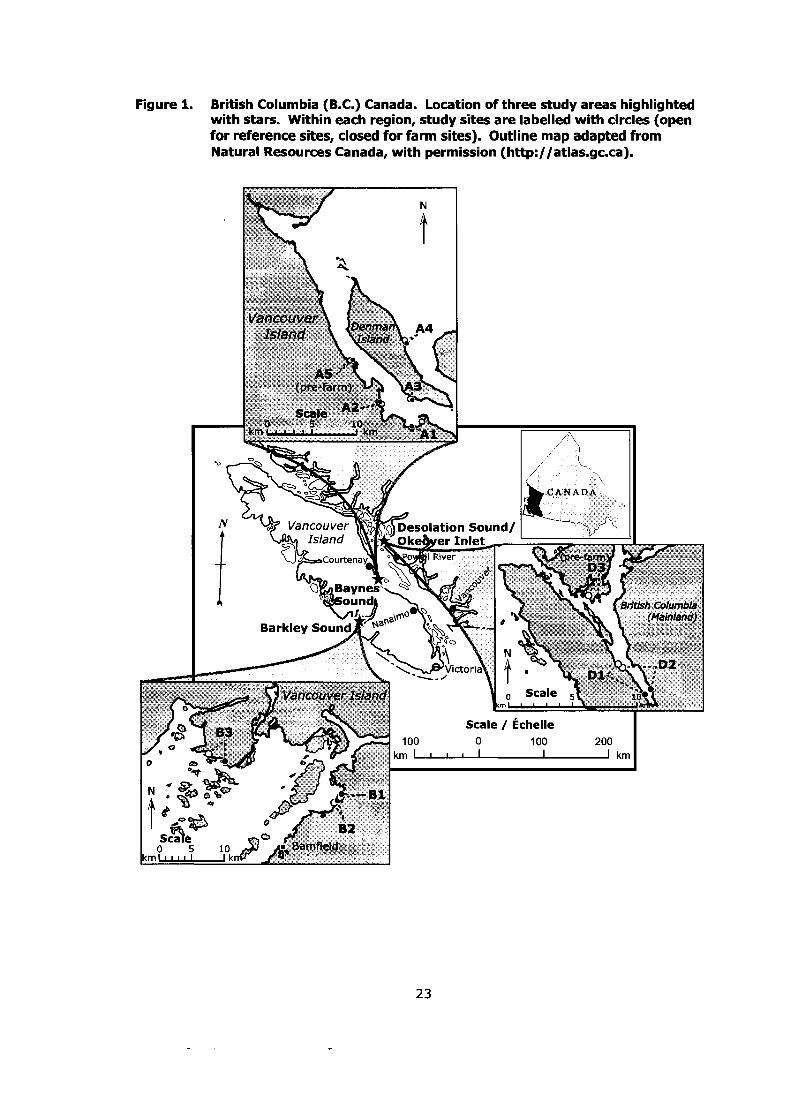
Figure 1. British Columbia (B.C.) Canada. Location of three study areas highlighted with stars. Within each region, study sites are labelled with circles (open for reference sites, closed for farm sites). Outline map adapted from Natural Resources Canada, with permission (http://atlas.gc.ca).
2.2 Field study
2.2.1 Study Sites
The principal component of this research is a large-scale field study.
Matched pairs of sites were sampled for species counts and environmental data
during daytime tides from May to August of 2003. Each pair of sites includes a
farm site, which was an active tenure employing the main practices of seeding
and netting, and a matched reference site, which was intended to be similar to
the farm site in most respects, apart from the lack of past or present aquaculture
activity.
Site pairs are referred to with a two-digit label, beginning with a letter,
denoting their regional location (A = Baynes Sound, B = Barkley Sound, D =
Desolation sound / Okeover Inlet), and a number, applied to sites in no particular
order within each region. Within each pair, farm and reference sites may be
differentiated by a suffix ("-F" = farm, "-R" = reference), although the same 2-
digit label is used to denote the pairwise relationship. The approximate location
of each site is shown in Figure 1. Site characteristics and sample sizes are listed
in Table 1.
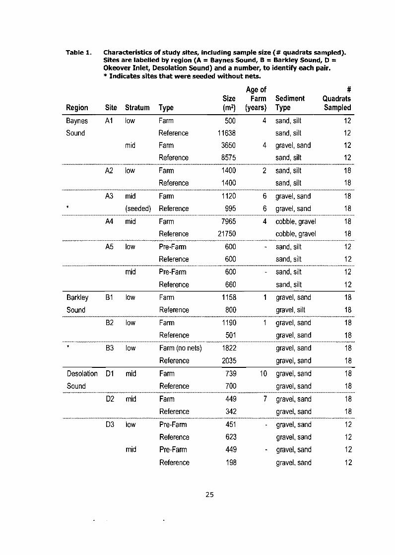
Table 1. Characteristics of study sites, including sample size (# quadrats sampled). Sites are labelled by region (A = Baynes Sound, B = Barkley Sound, D = Okeover Inlet, Desolation Sound) and a number, to identify each pair. * Indicates sites that were seeded without nets.
Age of # Size Farm Sediment Quadrats
Region Site Stratum Type (m2) (years) Type Sampled
Baynes A1 low Farm 500 4 sand, silt 12
Sound Reference 1 1638 sand, silt 12
mid Farm 3650 4 gravel, sand 12
Reference 8575 sand, silt 12
A2 low Farm 1400 2 sand, silt 18
Reference 1400 sand, silt 18
A3 mid Farm 1120 6 gravel, sand 18 * (seeded) Reference 995 6 gravel, sand 18
A4 mid Farm 7965 4 cobble, gravel 18
Reference 21750 cobble, gravel 18 . . . . . . . . . . . . . . . . . . . . . . . . . . . . . . . . . . . . . . . . . . . . . . . . . . . . . . . . . . . . . . . . . . . . . . . . . . . . , . . . , . . . . . . . . . . . . . . . . . . . . . . . . . . . . . . . . . . . . . . . . . . . . . . . . . . . . . . . . . . . . . . . . . . . . . . . . . . . . . . . . . . . . . . . , . . . . . . . . . . . . . . . . . . . . . . . . . . . . . . . . . . . . . . . . . . . . . . . . . . . . . . . . . . . . . . A5 low Pre-Farm 600 - sand, silt 12
Reference 600 sand, silt 12
mid Pre-Farm 600 - sand, silt 12
Reference 660 sand, silt 12
Barkley B1 low Farm 1 158 1 gravel, sand 18
Sound Reference 800 gravel, silt 18
B2 low Farm 1190 1 gravel, sand 18
Reference 50 1 gravel, sand 18 . . .. .. . .. . . . . . . . . . . . . . . . . . . . . . . . . . . . . . . . . . . . . . . . . . . . . . . . . . . . . . . . . . . . . . . . . . . . . . . . . . . . . . . . . . . . . . . . . .. . . . . . . . . . . . . . . . . . . . . . . . . . , . . . . .. . ... . . . . . . . . . . . . . . . . . . . . . . . . . . . . . . . . . . . . . . . . . . . . . . . . . . . . . . .. . . .. ... . . . . .. . . . .. . . . . . . . . . . . .. . . . . . . . . . * B3 low Farm (no nets) 1822 gravel, sand 18
Reference 2035 gravel, sand 18
Desolation D l mid Farm 739 10 gravel, sand 18
Sound Reference 700 gravel, sand 18
D2 mid Farm 449 7 gravel, sand 18
Reference 342 gravel, sand 18
D3 low Pre-Farm 451 - gravel, sand 12
Reference 623 gravel, sand 12
mid Pre-Farm 449 - gravel, sand 12
Reference 198 gravel, sand 12
Reference sites were selected from available nearby sites to match a
paired farm site with respect to sediment type (assessed visually, see below),
slope, size, wave exposure and approximate salinity. Farm sites were selected
based on permission from the owners, and the availability of a suitable reference
site. This type of observational sampling also integrates changes in response to
aquaculture practices over the entire history of the site, including 1 - 10 years of
aquaculture activity, depending on the site (see Table 1). This study did not
include the largest clam aquaculture leases currently active in B.C., therefore the
results are only reflective of the relatively small-scale aquaculture tenures that
were sampled.
A paired design also allows comparisons that account for site differences
between pairs, and should therefore help to control spatial variability that has
confounded intertidal experiments in the past (see Beal etal. 2001, Richards et
al. 1999, Sewell 1996). By matching reference and farm sites as closely as
possible, we hope to control for factors such as sediment type, beach slope, size,
wave exposure, and average temperature, which is assumed to be approximately
equal within each matched pair. The most important difference between each
farm and reference site within pairs is the application of seeding and netting to
the farm sites. Because both seeding and netting are present together on farm
sites in this study, it is difficult to tease apart the relative contribution of these
two practices to any observed differences. This study is primarily concerned with
the combined, cumulative effects associated with these two practices used
toget her.
Site B3-farm, and A3-reference were the only sites sampled that did not
use protective netting over seeded clam areas. The owner of the B3-farm lease
reported that this farm site was rarely visited by scoters, which did appear
frequently at the matched reference site chosen for this study. Such a small
sample size does not permit a rigorous comparison of the relative effects of
seeding and netting between treatment groups. Nevertheless, data from these
sites are reported for tentative comparison, and in the event it can be used in
conjunction with data collected in the future.
Although harvesting is also a possible source of disturbance that can
affect intertidal community structure, nearly all reference sites were also exposed
to recreational and commercial wild harvesting, as well as unknown levels of
poaching (personal observation). It is therefore assumed in this study that the
physical disturbance of digging associated with bivalve harvesting is similar
between farm and reference sites.
The only exception to this was one reference site (D2), which was located
in an area closed to shellfish aquaculture, within 1OOm of a public dock. High
public traffic may have discouraged any form of harvesting, including poaching,
in this area. The absence of anthropogenic bivalve removal at this site makes it
anomalous in the context of this study, although it also provides an example of a
possible "true baseline" state of an intertidal habitat in the absence of shellfish
harvesting.
Two "farm" sites sampled had been selected for future clam aquaculture,
although no aquaculture activity had started as of the time of sampling: A5 and
D3. These sites were sampled for baseline data with the intention to follow-up
and sample again once aquaculture practices such as seeding and netting had
been applied to the site. Unfortunately, such practices had not started at either
site in time to include follow-up data in this project. Nevertheless, data from
these sites is included to address whether sites chosen for shellfish aquaculture
were already different from reference sites, independent of aquaculture
practices. Such baseline data is also useful if these sites are ever sampled again,
to make more direct comparisons.
2.2.2 Sampling methodology
Sampling methods were based on those developed by Gillespie &
Kronlund (1999) for intertidal clam sampling, but adapted for sampling a range
of clam species. Only the infaunal bivalve data from the field study was included
and reported here. All field data and samples were collected between May and
August 2003.
Sites were stratified by tide height; areas between 1 and 2 metres above
chart datum were classified as "low", and areas above 2 metres were classified
as "mid". The highest points sampled in this study were at 2.7 metres above
chart datum. Average tides in the Barkley Sound region were much lower than
in the other regions, so stratum boundaries were shifted 0.5 m lower, to include
intertidal areas where netting is currently used in this region. Areas of netting
set the practical boundaries and limits of sampling on the farm beaches. Paired
reference beaches were laid out similarly to match the farm site according to size
of area and tidal range, within patches of similar sediment type and habitat.
Quadrats were placed randomly within each stratum at each beach (see
Table 1 for sample sizes). A stainless steel square frame (0.5 x 0.5 x 0.3 m
deep) was inserted into the sediment to isolate the quadrat area to be sampled.
Sediment was removed using a shovel, to a depth of 20 cm, and sifted through a
6 mm mesh to remove fine particles. A sub-sample of sediment (0.25 x 0.25 m)
within the top-right corner of each quadrat was also passed through a 1 mm
mesh sieve, under the 6 mm sieve, to capture smaller individuals. Sediment
retained in each sieve was also hand-sifted to locate organisms.
All individuals were identified in the field to the lowest taxonomic level
possible, usually species. If a pair of species was difficult to tell apart, for
example small Macoma obliqua or M. inquinata, individuals were assigned to a
default species (M. inquinata), unless clear diagnostic features identified them as
the other species. Field guides were used for initial identification (Harbo 1997,
Jensen 1995, Sept 1999), but difficult or unknown specimens were placed in
plastic or glass vials and stored in ethanol for later identification using further
resources (e.g. Kozloff 1983, Kozloff and Price 1987), or invertebrate experts
(e.g. the Bamfield Marine Sciences Centre, in Bamfield, B.C.). At one-third of the
quadrats from each site, the blotted wet weight of individual bivalves was
recorded to the nearest 0.1 g, before being returned to the sediment.
The position of each quadrat was recorded, relative to a reference point
on the beach, as well as tide height and qualitative sediment type. The height of
each quadrat above the water was measured using Abney levels and a
measuring tape (Giles 1971). Tide predictions from the Canadian Hydrologic
Service were used to obtain the height of the water at the time of the height
measurement. These two heights were added to obtain an approximate height
above chart datum for any point on the beach. A similar method was used to
locate stratum boundaries, usually by marking the height of the water at a
specified time from tidal predictions to locate pre-defined heights. It was found
through experience that the Abney levels were only accurate within a distance of
approximately 30m, which is within the range of many commercial laser levels of
similar cost, although simply following the water level on an incoming tide and
noting the time of submersion was often adequate for determining tidal
elevation. The sediment type at each quadrat was assessed qualitatively by
recording the two most abundant particle size classes present in the sediment
(Wentworth 1922).
2.2.3 Statistical Treatment and Analysis
For the field study, only the infaunal bivalve (clam) data from the sampled
communities were included for analysis. For each quadrat, counts of smaller
individuals, from the 0.25 x 0.25 m sub-sample, were multiplied by 4 to
normalize by area, and added to counts of larger individuals from the 0.5 x 0.5 m
quadrat. For each estimate, paired t-tests were used to assess consistent
differences between farm and reference sites. Differences within each pair were
weighted by the inverse of a pooled estimate of within-site standard error, if
available (for differences in mean density, for example, but not indices of
diversity). All statistical comparisons and tests were calculated using a pooled
estimate of variance across the low and mid strata, allowing for differences
between strata, and a significance level of 0.05. Equality of variance between
farm and reference sites was also tested, over all tide heights, for each estimate
used. Equality of variances is not required for a paired test, but some results
indicated definite patterns among paired differences that might be explained by
changes in between-site variation within treatments.
Estimates of species richness and diversity indices were calculated using
the Estimates software program (Colwell 1997). There is an ever-growing list of
possible estimators to use to compare species richness, but few of them have
been well-characterized and there is much disagreement over which estimators
are better in which situation, although non-parametric estimators may be more
accurate and precise (Brose et al. 2003, see Colwell 1997 for formulae and
references, Foggo etal. 2003, Hellmann and Fowler 1999, Purvis and Hector
2000). While some estimators are better at reducing bias, others have higher
precision. For this study, estimating the true number of species (reducing bias)
is less important than the ability to discriminate between estimates (high
precision). The first-order Jackknife estimator (Jack-1) has been well
characterized for a long period throughout the literature (Burnham and Overton
1978, 1979, Heltshe and Forrester 1983, 1985) and consistently found to be a
relatively precise estimator, which can also reduce bias at small sample sizes
(Brose et al. 2003, Foggo etal. 2003, Hellmann and Fowler 1999). Newer
coverage-based estimators developed by Anne Chao (Chao et al. 2000, Chao and
Lee 1992, Chao and Yang 1993, Chazdon et a/. 1998) have shown promise,
although the incidence-based version (ICE) seems to perform better than its
abundance-based sibling (ACE) (Brose et a/. 2003, Foggo et a/. 2003). Other
estimators were found in our data to be either less precise than those already
mentioned, or theoretically inappropriate.
Both the Jackknife and ICE estimators are incidence-based, which means
they extrapolate the number of estimated species based on the incidence of
observed species within a collection of repeated samples (quadrats). Such
estimators are potentially sensitive to changes in spatial distribution, or
patchiness (Brose et al. 2003, Foggo et al. 2003). A decrease in patchiness may
result in a lower estimate of species richness, independent of any actual change
in the number of species present at a site. This was the primary reason for also
comparing sites using the abundance-coverage estimator (ACE). No single
estimator in this case could be argued convincingly to be "the best", so results
were compared using all three proposed estimators as a method of assessing
how robust they are.
Sites were also compared with respect to community evenness, using
Simpson's evenness index, and heterogeneity, calculated using the Shannon-
Weiner function (see Krebs 1999). Heterogeneity is a composite measure
incorporating richness and community evenness, often termed "diversity".
Observed changes in such a composite measure are difficult to interpret, which is
why it is important and an increasingly popular practice to separate diversity into
measures of richness and evenness. The Shannon-Weiner function is included
here primarily to allow comparison with other studies that have used only this
univariate index of diversity.
Multivariate comparisons of communities were performed using the
PRIMER software. Five of the species sampled were unidentified, and observed
only once or twice at individual sites. These species were excluded from the
multivariate analysis because they would contribute little information and their
unidentified status could complicate the interpretation of results. Measures of
species weights and counts were converted to an average biomass and density
per square metre, to standardize for different sample sizes. Density and biomass
data were analyzed separately. Similarity matrices were calculated using the
Bray-Curtis index of similarity (see Legendre and Legendre 1998) on fourth-root
transformed data, which was used to draw an MDS plot (non-metric Multi-
Dimensional Scaling).
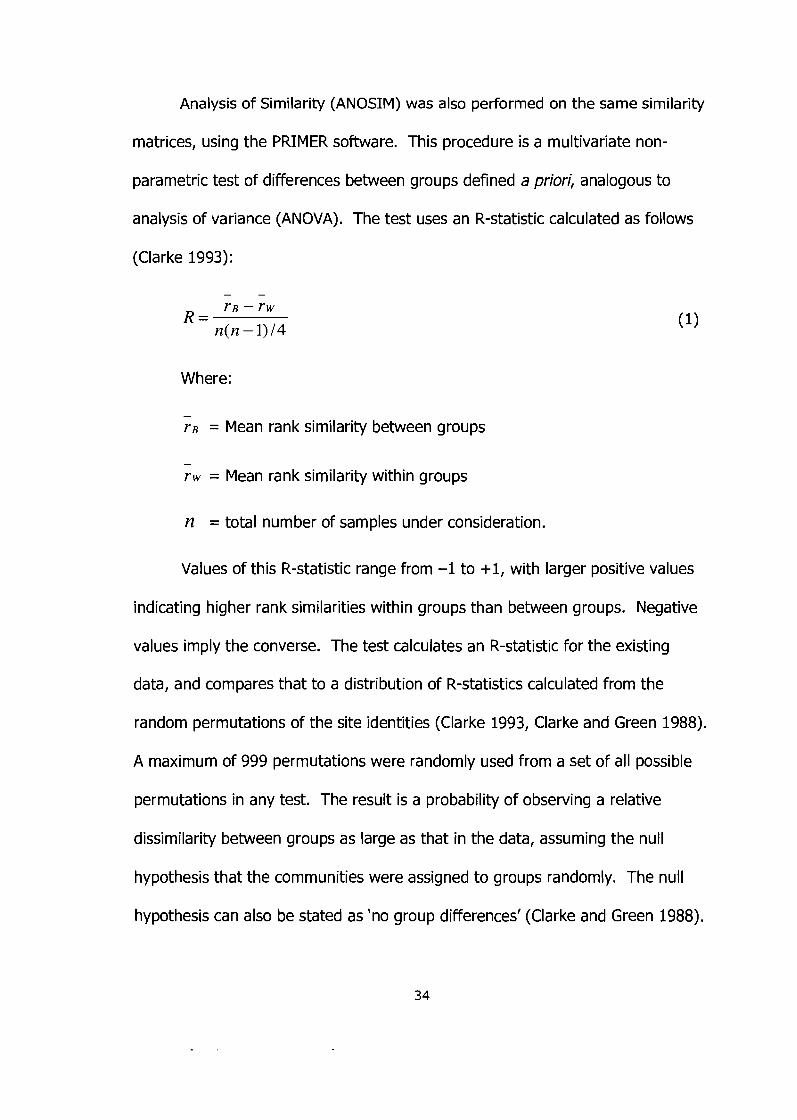
Analysis of Similarity (ANOSIM) was also performed on the same similarity
matrices, using the PRIMER software. This procedure is a multivariate non-
parametric test of differences between groups defined a priori, analogous to
analysis of variance (ANOVA). The test uses an R-statistic calculated as follows
(Clarke 1993):
Where:
- re = Mean rank similarity between groups
- rw = Mean rank similarity within groups
n = total number of samples under consideration.
Values of this R-statistic range from -1 to +I, with larger positive values
indicating higher rank similarities within groups than between groups. Negative
values imply the converse. The test calculates an R-statistic for the existing
data, and compares that to a distribution of R-statistics calculated from the
random permutations of the site identities (Clarke 1993, Clarke and Green 1988).
A maximum of 999 permutations were randomly used from a set of all possible
permutations in any test. The result is a probability of observing a relative
dissimilarity between groups as large as that in the data, assuming the null
hypothesis that the communities were assigned to groups randomly. The null
hypothesis can also be stated as 'no group differences' (Clarke and Green 1988).
We tested for differences among types (farm or reference) and tide height
strata (low or mid-intertidal) in a two-factor crossed analysis. This method tests
for differences in each factor, averaged over all levels of the second factor
(Clarke 1993). Tests for differences between regions were performed as a 2-
way crossed analysis with type (farm or reference), if sites did not significantly
differ by any other factor. Differences by region and tide height are somewhat
confounded, as some regions did not include sites in all tide height strata, so
some combinations of region and stratum do not exist. I n the absence of
significant differences for any other factor, regional differences would indicate
that community structure is more strongly determined by local factors that vary
by region (salinity, water currents, temperature, etc.), as opposed to the broader
factors of tide height and farming practices.
Sites that were sampled under pre-farming conditions (A5 and D3) were
included in these analyses as additional reference sites. The two sites sampled
that had been seeded but not netted (A3 reference and 83 farm) were excluded,
because only two sites did not allow for a statistically rigorous comparison of this
treatment with others. We focused instead on the combined practices of seeding
and netting (farm sites), as compared to reference sites where these activities
were absent.
2.3 Netting Experiment
A small, pilot experiment was conducted to examine any possible short-
term effects of predator exclusion, using nets typically used in industry. The
short duration of the experiment (see below) did not allow for possible changes
in community structure as a result of recruitment or competitive differences
between treatments, but the goal was to observe whether or not prey depletion
in control plots also occurred under netted plots.
2.3.1 Study Sites and Treatment Structure
Three study sites were chosen within Baynes Sound (see Figure 2),
labelled using an abbreviation of a name of the location. At each site, the
netting treatment was applied randomly to one plot within each pair, with the
other left uncovered. Each plot pair consisted of two square plots, 5 x 5 m in
area, separated by 2m to reduce edge effects between treatments. Each plot
was arranged beside its pair, parallel to the water's edge. At each site, one pair
of plots was set at 3.0 m above chart datum (labelled 'A" stratum) and a second
pair at 2.5m r B " stratum). This design resulted in three (3) replicate treatment
and control pairs at each site and tide height combination.
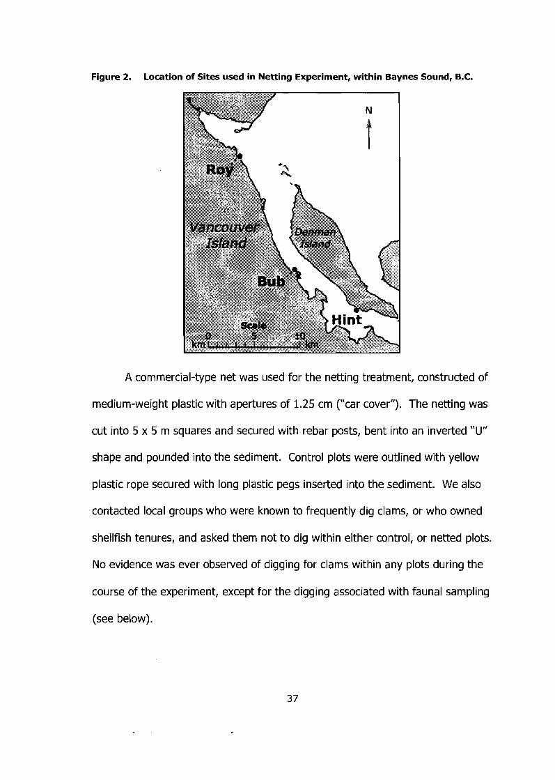
Figure 2. Location of Sites used in Netting Experiment, within Baynes Sound, B.C.
A commercial-type net was used for the netting treatment, constructed of
medium-weight plastic with apertures of 1.25 cm ("car cover"). The netting was
cut into 5 x 5 m squares and secured with rebar posts, bent into an inverted "U"
shape and pounded into the sediment. Control plots were outlined with yellow
plastic rope secured with long plastic pegs inserted into the sediment. We also
contacted local groups who were known to frequently dig clams, or who owned
shellfish tenures, and asked them not to dig within either control, or netted plots.
No evidence was ever observed of digging for clams within any plots during the
course of the experiment, except for the digging associated with faunal sampling
(see below).
2.3.2 Sampling methodology
Sampling protocols for the netting experiment are similar in most ways to
the field study (see above), except as follows. Quadrats used were the same
size (50 x 50 cm x 30cm deep), and five quadrats were sampled randomly within
each plot, accounting for approximately 5% of the total surface area of each
plot. It was determined that the amount of time required to sieve down to 1 mm
was too costly compared to the small amount of information gained (see
Appendix B). Therefore, sediment within each quadrat was sieved through only
a 6 mm wire mesh sieve.
Each plot was sampled at three separate times during the course of the
experiment. The first was during October, 2003 (time = 0), as a baseline state
prior to the addition of the netting treatment. Plots were sampled a second time
during May of 2004 (time = I), and again near the end of August, 2004 (time =
2). Each sampling period lasted about 10 days.
2.3.3 Statistical Treatment and Analysis
The netting experiment carried out over a period of 10 months was
designed as a small-scale pilot experiment, with the goal of measuring depletion
by predators over a winter, and the following summer season. I f the nets
prevented predation from large epibenthic predators such as scoters, crabs, or
fish, it is predicted that areas of beach under randomly-assigned netted plots
would show less reduction in prey faunal densities than nearby areas without
netting. I n the context of the paired plots used in this experiment (see above),
the difference in faunal density within pairs (net - control) is expected to be
larger (more positive) after a season, than it was during the baseline, initial
sampling period.
Because the experiment was designed with treatment grouped into pairs,
a difference was calculated for each paired plot (net value - control value) for
each variable of interest, and these differences were used in a repeated
measures analysis (Sokal and Rohlf 1981) to examine significant linear changes
through time, accounting for possible differences between tide height strata.
JMP software was used to perform the repeated measures analysis.
The first sampling period (t=O) collected data before any netting
treatment was applied, therefore the average difference for this time period is
not a result of any experimental treatment effects. The average difference
between plots may not be zero for the baseline sampling period, by chance, but
the repeated measures analysis examines how this average difference changes
once the netting treatment is applied to one plot within each pair.
Species counts at each quadrat were converted to density values
(individua1s.m-2, by multiplying counts by four (4) to scale the area of the
quadrat (0.25 m2) to 1.0 m2. Sample sizes were equal among all plots, but this
conversion allows values to be compared with other research presented herein,
and other published data. Mean densities for each plot (net or control), over five
quadrats, were computed at each sampling period, and used to analyze changes
in faunal density associated with netting similar to that used in commercial clam
aquaculture in B.C.
Faunal densities were grouped by simple ecological roles:
Epifauna
Predatory Infauna
Non-predatory Infauna (Including Infaunal Bivalves)
Venerupis philippinarum
The last group includes only the commercial species, V. philippinarum,
which was analyzed separately to allow a comparison with data from other
sources, including the field study presented in this work. This species is also
very abundant and often the dominant species within bivalve communities, and
even non-predatory infauna at some sites. Therefore, some groups (infaunal
bivalves, non-predatory infauna, total infauna) were re-analyzed with V.
philippinarum excluded .
Species richness, evenness, and diversity were calculated in an identical
manner as for the field study data (see above), and examined using repeated
measures analysis of the differences between net and control plots, as described
above.
Multivariate analysis of communities was carried out using the same
software and general methods as for field study data (see above), although the
analysis was changed to match the treatment structure of the experiment. A
matrix was constructed with counts of each species pooled across five quadrats,
for each plot and sampling period. A similarity matrix was then calculated for
each plot, at each sampling period, using the Bray-Curtis index of similarity,
based on fourth-root transformed data. This similarity matrix was used to
construct MDS plots, and perform Analysis of Similarity (ANOSIM).
ANOSIM was performed to test hypotheses concerning differences among
levels of various factors. At each sampling period, a two-way ANOSIM was used
to test for differences between treatment levels (net, control plots), crossed with
tide height stratum. No difference was predicted for t=O (baseline), since no
netting had been applied, but a difference was predicted for either t= l , or t=2,
or both. A second approach was used to test temporal changes, in a way that
would be analogous to the repeated measures analysis for a single variable
described above. A one-way ANOSIM was used to test differences between time
periods (each pair), within each treatment level (net and control). If none of
these tests showed any significant changes, other factors were examined to
explore which ones could explain the majority of the structure in the MDS plots
(see Results, below).
Results are presented separately for each community studied: Infaunal
bivalve component of the field study, and netting experiment (whole
community).
3.1 Field Study - lnfaunal Bivalve Community
3.1.1 Pre-Farm Sites
A summary of bivalve data from pre-farm sites and paired reference sites
is presented in Table 2. In terms of bivalve density, the farm and reference sites
within the D3 pair appear no different. The A5 pre-farm site in the low stratum,
however, has a higher mean density of Venerupis philippinarum, lower density of
other bivalves, but similar total bivalve density as the paired reference site. The
biomass of V. philippinarum, however, is no different between the pre-farm and
reference site at A5, but the D3 pre-farm site appears to have lower biomass of
this species than the paired reference site.
There is also a remarkable lack of consistency between these site pairs
with respect to differences in species richness, diversity and evenness (see Table
24). I n some cases, values are higher on the pre-farm site, others are very
similar, or even lower.
This data demonstrates that some farmed sites may differ inherently from
reference sites, particularly in the case of species of commercial interest. Some
sites selected for clam farming, on the other hand, may be very similar to other
sites in terms of pre-existing biotic conditions.
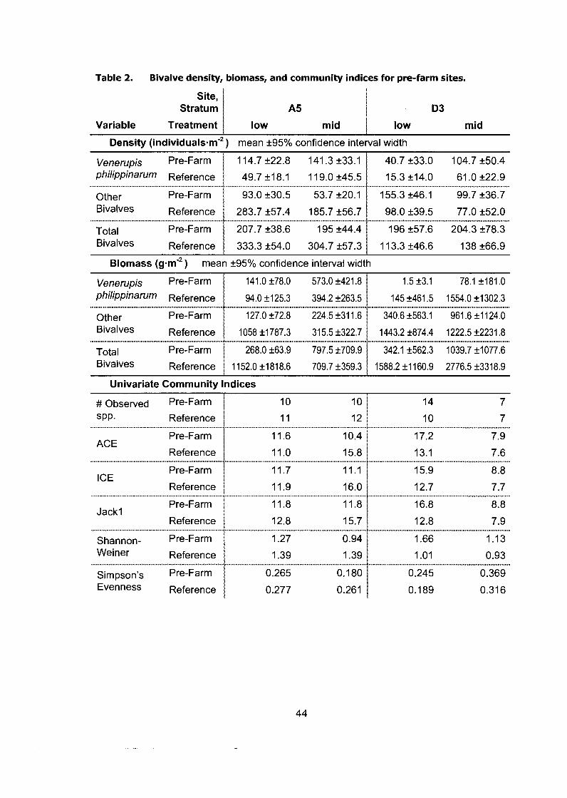
Table 2. Bivalve density, biomass, and community indices for pre-farm sites.
Site, Stratum A5 D3
Variable Treatment low mid low mid
Density (individuals-m-2) mean k95% confidence interval width
Venerupis Pre-Farm 114.7 k22.8 141.3 k33.1 40.7 k33.0 104.7 k50.4 philippinarum Reference 49.7 k1 8.1 1 19.0 k45.5 15.3 k14.0 61 .O k22.9
Other Pre-Farm 93.0 k30.5 53.7 k20.1 99.7 k36.7
Bivalves Reference 283.7 k57.4 1 85.7 k56.7 77.0 k52.0
Total Pre-Farm 207.7 k38.6 1 95 k44.4 196 k57.6 204.3 k 78.3 Bivalves Reference / 333.3 k54.0 304.7 k57.3 138 k66.9
Biomass (g-m") mean k95% confidence interval width
philippinarum Reference t 94.0 k125.3 394.2 k263.5 ...................................................................................................................................................... .............................................................................. 145 k461.5 1554.0 k1302.3
Other Pre-Farm 127.0 k72.8 224.5 k311.6 340.6 k563.1 961.6 k1 124.0 Bivalves 1058 k1787.3 31 5.5 k322.7 1443.2 k874.4 1222.5 k2231.8
........................................... .............................................................................. .............................................................................. Total 268.0 k63.9 797.5 k709.9 342.1 k562.3 1039.7 k1077.6 Bivalves Reference / 1152.0 k1818.6 709.7 k359.3 1588.2 k1160.9 2776.5 k3318.9
Univariate Community Indices
# Observed Pre-Farm 10 10 14 7
SPP- Reference 11 12 10 7
Pre-Farm 11.6 10.4 17.2 7.9 ACE
Reference 11.0 15.8 13.1 7.6
Pre-Farm 11.7 11.1 15.9 ICE
8.8
Reference 11.9 16.0 12.7 7.7
Pre-Farm
Reference
Shannon- Pre-Farm 1.27 0.94 1.66 1.13
Weiner Reference 1.39 1.39 1.01 0.93
simpson's Pre-Farm 0.265 0.180 0.245 0.369 Evenness Reference 0.277 0.261 0. 189 0.31 6
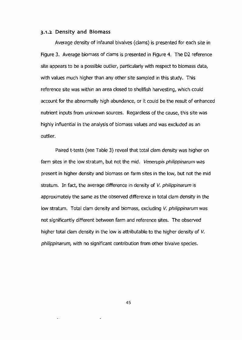
3.1.2 Density and Biomass
Average density of infaunal bivalves (clams) is presented for each site in
Figure 3. Average biomass of clams is presented in Figure 4. The D2 reference
site appears to be a possible outlier, particularly with respect to biomass data,
with values much higher than any other site sampled in this study. This
reference site was within an area closed to shellfish harvesting, which could
account for the abnormally high abundance, or it could be the result of enhanced
nutrient inputs from unknown sources. Regardless of the cause, this site was
highly influential in the analysis of biomass values and was excluded as an
outlier.
Paired t-tests (see Table 3) reveal that total clam density was higher on
farm sites in the low stratum, but not the mid. Venerupis philippinarum was
present in higher density and biomass on farm sites in the low, but not the mid
stratum. I n fact, the average difference in density of V. philippinarum is
approximately the same as the observed difference in total clam density in the
low stratum. Total clam density and biomass, excluding V. philippinarum was
not significantly different between farm and reference sites. The observed
higher total clam density in the low is attributable to the higher density of V.
philippinarum, with no significant contribution from other bivalve species.
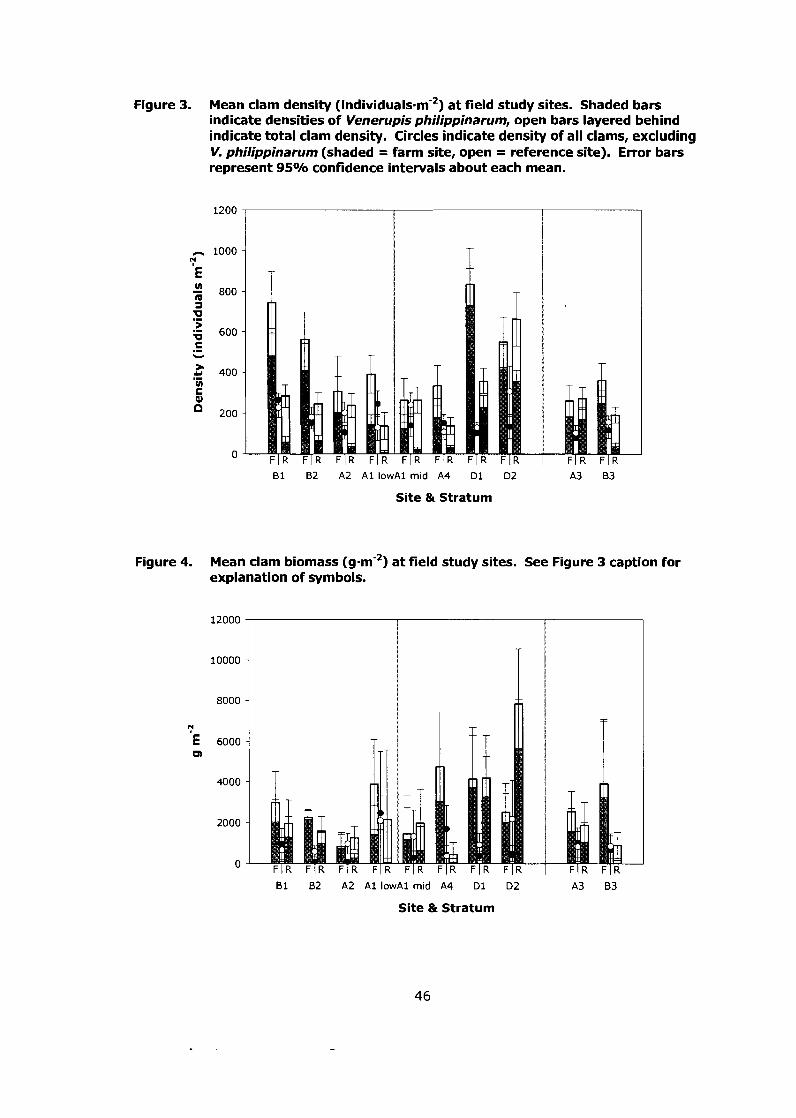
Figure 3. Mean clam density (individuals-m-2) at field study sites. Shaded bars indicate densities of Venerupis philippinarum, open bars layered behind indicate total clam density. Circles indicate density of all clams, excluding V. philippinarum (shaded = farm site, open = reference site). Error bars represent 95% confidence intervals about each mean.
8 1 82 A2 A1 lowAl mid A4 D l D2
Site & Stratum
Figure 4. Mean clam biomass (g.m-2) at field study sites. See Figure 3 caption for explanation of symbols.
6 1 B2 A2 A1 lowAl mid A4 D l D2
Site & Stratum
Table 3. Results of weighted paired analyses of bivalve abundance, including Mean Difference (Farm-Reference) f 95% confidence interval width (with degrees of freedom), for each estimate. Mean differences significantly different from zero (2-tailed) are highlighted in bold, with *. Site D2, in the mid stratum, was highly influential in tests using biomass data and a potential outlier, so was omitted from the calculation.
Low Stratum
Mean Difference
Test (F-R) f 95% CI p-value
Density (individuals-m-2) (df = 6)
Total clams 279.6 f 241.6 0.030*
Venerupis philippinarum 227.0 f 176.4 0.020*
Other clams (V. philippinarum excluded) -2.1 k100.5 0.960
Biomass (g-m'2) (df = 5d)
Total clams 444 k1698.0 0.531
Venerupis philippinarum 872.9 f 792.9 0.037*
Other clams ( V. philippinarum excluded) -452.3 k852.1 0.231
Mid Stratum
Mean Difference
(F-R) f 95% CI p-value
Unequal Variance (F-test)
Although the biomass of other clams (excluding V. philippinarum) was, on
average, lower at farm sites, the low sample sizes and between-site variability
created noise larger than this signal. It seems unlikely that that there is no
change in abundance of other bivalves, if total clam abundance does not change
(density in the mid, biomass in both strata), and the commercial species is more
abundant on farm sites. I n the presence of greater density and biomass of V.
philippinarum on farm sites, either total bivalve abundance must increase by a
corresponding amount, or the abundance of other species must decline, or some
combination of both.
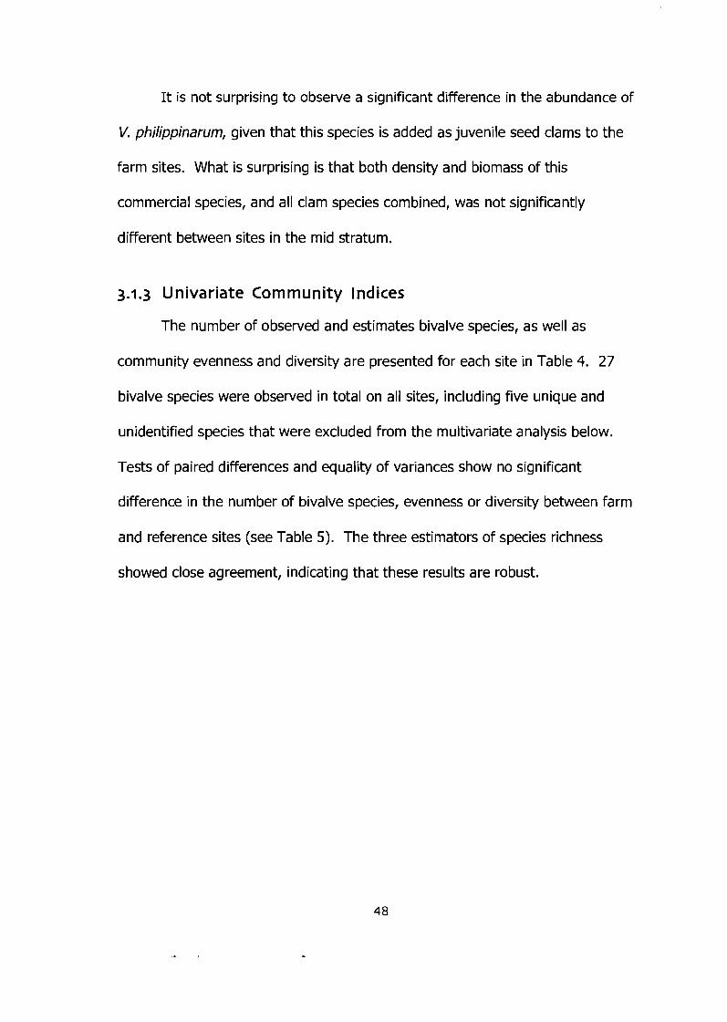
It is not surprising to observe a significant difference in the abundance of
V. philippinarum, given that this species is added as juvenile seed clams to the
farm sites. What is surprising is that both density and biomass of this
commercial species, and all clam species combined, was not significantly
different between sites in the mid stratum.
3.1.3 Univariate Community Indices
The number of observed and estimates bivalve species, as well as
community evenness and diversity are presented for each site in Table 4. 27
bivalve species were observed in total on all sites, including five unique and
unidentified species that were excluded from the multivariate analysis below.
Tests of paired differences and equality of variances show no significant
difference in the number of bivalve species, evenness or diversity between farm
and reference sites (see Table 5). The three estimators of species richness
showed close agreement, indicating that these results are robust.
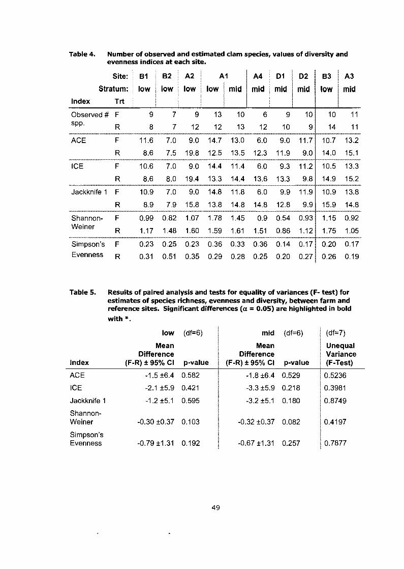
Table 4. Number of observed and estimated clam species, values of diversity and evenness indices at each site.
ACE F 11.6 7.0 9.0 14.7 13.0 6.0 9.0 11.7
R 8.6 7.5 19.8 12.5 13.5 12.3 11.9 9.0 ............................................................................................................................................................................................. ICE F 10.6 7.0 9.0 14.4 11.4 6.0 9.3 11.2
R 8.6 8.0 19.4 13.3 14.4 13.6 13.3 9.8 ............................................................................................................................................................................................. Jackknife 1 F 10.9 7.0 9.0 14.8 11.8 6.0 9.9 11.9
R 8.9 7.9 15.8 13.8 14.8 14.8 12.8 9.9 ............................................................................................................................................................................................. Shannon- F 0.99 0.82 1.07 1.78 1.45 0.9 0.54 0.93 Weiner 1.17 1.48 1.60 1.59 1.61 1.51 0.86 1.12 ............................................................................................................................................................................................. Sirnpson's F 0.23 0.25 0.23 0.36 0.33 0.36 0.14 0.17
Evenness R 0.31 0.51 0.35 0.29 0.28 0.25 0.20 0.27
Site: 61 1 62
Stratum: low low Index Trt
Table 5. Results of paired analysis and tests for equality of variances (F- test) for estimates of species richness, evenness and diversity, between farm and reference sites. Significant differences (a = 0.05) are highlighted in bold
with *. low (df=6)
Mean Difference
Index (F-R) f 95% CI p-value
ACE -1.5 k6.4 0.582
ICE -2.1 k5.9 0.421
Jackknife 1 -1.2 k5.1 0.595
Shannon- Weiner -0.30 k0.37 0.1 03
Sirnpson's Evenness -0.79 k1.31 0.192
Observed # F 9 7 9 13 10 6 9 10
SPP. R 8 7 12 12 13 12 10 9
A2 A I
mid (df=6) I (df=7)
A4 D l
mid . mid
10 11
14 11
low low
Mean I Unequal Difference i Variance
(F-R) f 95% CI p-value i (F-Test)
mid
D2
mid
63
low
A3
mid
3.1.4 Multivariate Analysis
MDS ordinations of sites are displayed in Figure 5 (Den,sity data) and
Figure 6 (Biomass data). The relatively high stresses in Figure 5 indicate that
individual relationships are poorly represented, but the overall ordination is
acceptable. Higher stresses in Figure 6 indicate a higher risk of misleading
interpretations, but is still within an acceptable range (Clarke 1993). When
Venerupis philippinarum was excluded from the analyses, the overall ordination
changed little for density data, apart from a small rotation evident in the MDS
plot, which is meaningless in this non-metric context. V. philippinarum appears
far more influential with regards to biomass data, where its absence reduces the
overall similarity among farm sites.
ANOSIM tests (see Table 6) found no significant differences in rank
similarities between farm and reference sites, in any crossed analysis. No
significant differences were found for any factor considered (tide height, region,
treatment) with respect to biomass data. I n terms of density, significant
differences between regions were apparent, regardless of the inclusion of V.
philippinarum in the analysis. More detailed tests reveal that these regional
differences are only significant within reference sites, but not within farm sites
(see Table 6).

Figure 5 (a & b). MDS Plot of average density (individualsmm-2, of clam species (a, stress = 0.18) and results of the same analysis, with Venerupis philippinarum excluded (b, stress = 0.19). Sites are identified by region (+ = Barkley sound, = Baynes Sound, . = Desolation Sound), stratum (black = low, grey = mid), and type (open = reference, closed = farm). Site labels ending in a dash (D3-, A5-) indicate "pre-farming" sites. Active farm sites have also been outlined in a dashed line within the reduced ordination space.
a) All Bivalve spp.
b) V. philippinarum excluded 0 A2
0 82
. . .4\81
O A S - ... \
_.- '$82 \ 0/ D2
* \ \ \ Cl \
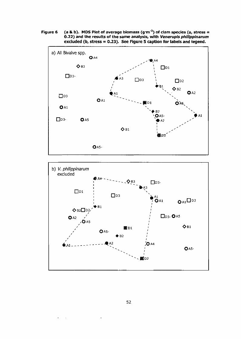
Figure 6 (a & b). MDS Plot of average biomass (gmm-') of clam species (a, stress = 0.22) and the results of the same analysis, with Venerupis philippinarum excluded (b, stress = 0.23). See Figure 5 caption for labels and legend.
a) All Bivalve spp. 0 A4
b) V, philippinarum excluded
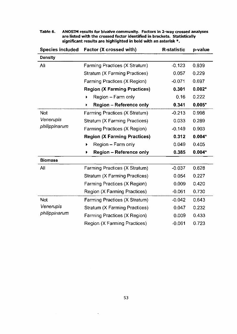
Table 6. ANOSIM results for bivalve community. Factors in 2-way crossed analyses are listed with the crossed factor identified in brackets. Statistically significant results are highlighted in bold with an asterisk *.
Species included Factor (X crossed with) R-statistic p-value
Density
All Farming Practices (X Stratum) -0.123 0.939
Stratum (X Farming Practices) 0.057 0.229
Farming Practices (X Region) -0.071 0.697
Region (X Farming Practices) 0.301 0.002*
Region - Farm only 0.16 0.222
Region - Reference only 0.341 0.005*
Not Farming Practices (X Stratum) -0.213 0.998 Venerupis Stratum (X Farming Practices) 0.033 0.289 philippinarum Farming Practices (X Region)
Region (X Farming Practices) 0.312 0.004*
b Region - Farm only 0.049 0.405
b Region - Reference only 0.385 0.004*
Biomass
All Farming Practices (X Stratum) -0.037 0.628
Stratum (X Farming Practices) 0.054 0.227
Farming Practices (X Region) 0.009 0.420
Region (X Farming Practices) -0.061 0.730
Not Farming Practices (X Stratum) -0.042 0.643 Venerupis Stratum (X Farming Practices) 0.047 0.232 philippinarum Farming Practices (X Region) 0.009 0.433
Region (X Farming Practices) -0.061 0.723
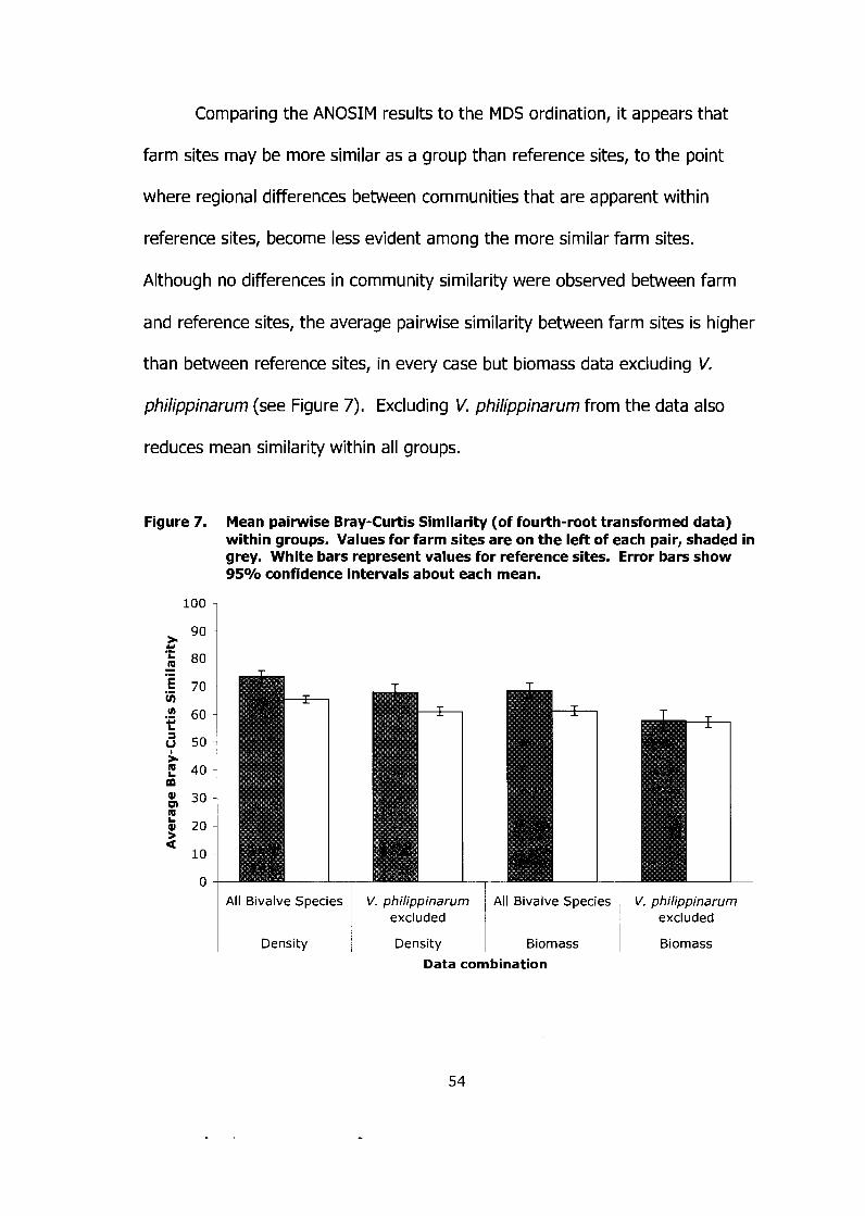
Comparing the ANOSIM results to the MDS ordination, it appears that
farm sites may be more similar as a group than reference sites, to the point
where regional differences between communities that are apparent within
reference sites, become less evident among the more similar farm sites.
Although no differences in community similarity were observed between farm
and reference sites, the average pairwise similarity between farm sites is higher
than between reference sites, in every case but biomass data excluding V.
philippinarum (see Figure 7). Excluding V. philippinarum from the data also
reduces mean similarity within all groups.
Figure 7.
100
* 90 u .- 80 - .-
E 70 .- ul .% 60 t 3 y 50 * 2 40 m & 30
5 20 2
10
0
Mean pairwise Bray-Curtis Similarity (of fourth-root transformed data) within groups. Values for farm sites are on the left of each pair, shaded in grey. White bars represent values for reference sites. Error bars show 95% confidence intervals about each mean.
Density 1 Density Biomass 1 Biomass
Data combination
All Bivalve Species V. philippinarum excluded
All Bivalve Species V. philippinarum excluded
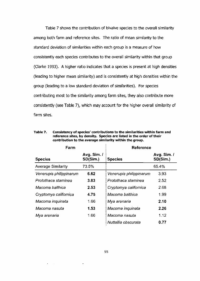
Table 7 shows the contribution of bivalve species to the overall similarity
among both farm and reference sites. The ratio of mean similarity to the
standard deviation of similarities within each group is a measure of how
consistently each species contributes to the overall similarity within that group
(Clarke 1993). A higher ratio indicates that a species is present at high densities
(leading to higher mean similarity) and is consistently at high densities within the
group (leading to a low standard deviation of similarities). For species
contributing most to the similarity among farm sites, they also contribute more
consistently (see Table 7), which may account for the higher overall similarity of
farm sites.
Table 7. Consistency of species' contributions to the similarities within farm and reference sites, by density. Species are listed in the order of their contribution to the average similarity within the group.
Farm
Species Avg. Sim. I SD(Sim.)
Average Similarity 73.5%
Venerupis philippinarum 6.62
Protothaca staminea 3.83
Macoma balthica 2.53
Cryptomya californica 4.75
Macoma inquinata 1.66
Macoma nasuta 1.53
Mya arenaria 1.66
Reference
Species Avg. Sim. I SD(Sim.)
Venerupis philippinarum
Protothaca staminea
Cryptomya californica
Macoma balthica
Mya arenaria
Macoma inquinata
Macoma nasuta
Nuttallia obscurata
Table 8 lists species in order of their contribution to the dissimilarity
between farm and reference sites by density data. There is no hypothesis test
as to whether or not densities of each species may differ between groups, but it
is apparent that no species is absent in one group or another, but vary slightly by
abundance between the two groups. Not surprisingly, the commercially seeded
species Venerupis philippinarum accounts for the largest single component of the
dissimilarity between farms and reference sites. Deposit feeders such as
Macoma nasuta, Nuttallia obscurata and Cryptomya californica seem to have
slightly lower densities on farm sites. Densities of smaller filter feeders such as
Macoma balthica and M. inquinata are higher on farm sites. Other species vary
by tide height and may have slightly higher densities on reference sites in the
mid, but higher farm densities in the low intertidal.
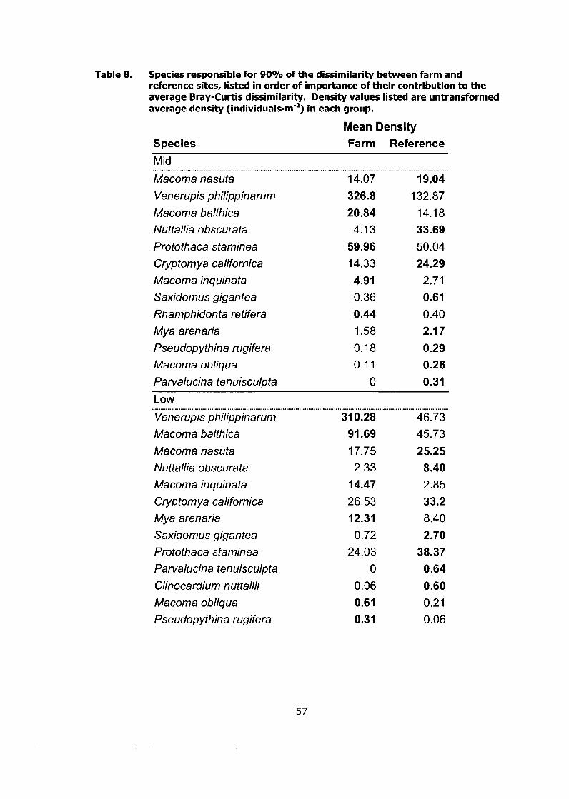
Table 8. Species responsible for 90% of the dissimilarity between farm and reference sites, listed in order of importance of their contribution to the average Bray-Curtis dissimilarity. Density values listed are untransformed average density (individualsmm-2, in each group.
Species Mean Density Farm Reference
Mid
Macoma nasuta
Venerupis philippinarum
Macoma balthica
Nuttallia obscurata
Protothaca staminea
Cryptomya californica
Macoma inquinata
Saxidomus gigantea
Rhamphidon ta re tifera
Mya arenaria
Pseudopythina rugifera
Macoma obliqua
Patvalucina tenuisculpta
Low ......................................................................... ...... .................................................................................... Venerupis philippinarum 31 0.28 46.73
Macoma balthica 91.69 45.73
Macoma nasuta 17.75 25.25 Nuttallia obscurata 2.33 8.40 Macoma inquinata
Cryptomya californica
Mya arenaria
Saxidomus gigantea
Protothaca staminea 24.03 38.37 Patvalucina tenuisculpta 0 0.64 Clinocardium nuttallii 0.06 0.60 Macoma obliqua
Pseudopythina rugifera
Table 9 lists species in order of their contribution to the dissimilarity
between farm and reference sites by biomass data. Once again, Venerupis
philippinarum is responsible for most of the dissimilarity. Otherwise, the order of
species in Table 9 is generally the opposite of Table 8. Larger species contribute
more to differences in biomass, but are so numerically uncommon that they
contribute very little in terms of density. The opposite is true for smaller, more
abundant species. Not only are species such as V. philippinarum, P. staminea
and M. inquinata present in higher densities on farm sites, their biomass is also
higher. Although M. balthica was less dense on farm sites, the total biomass is
higher, suggesting a possible change in body size demographics for this species
on farm sites. The reverse pattern is observed for Mya arenaria, which may be
smaller on farm sites.
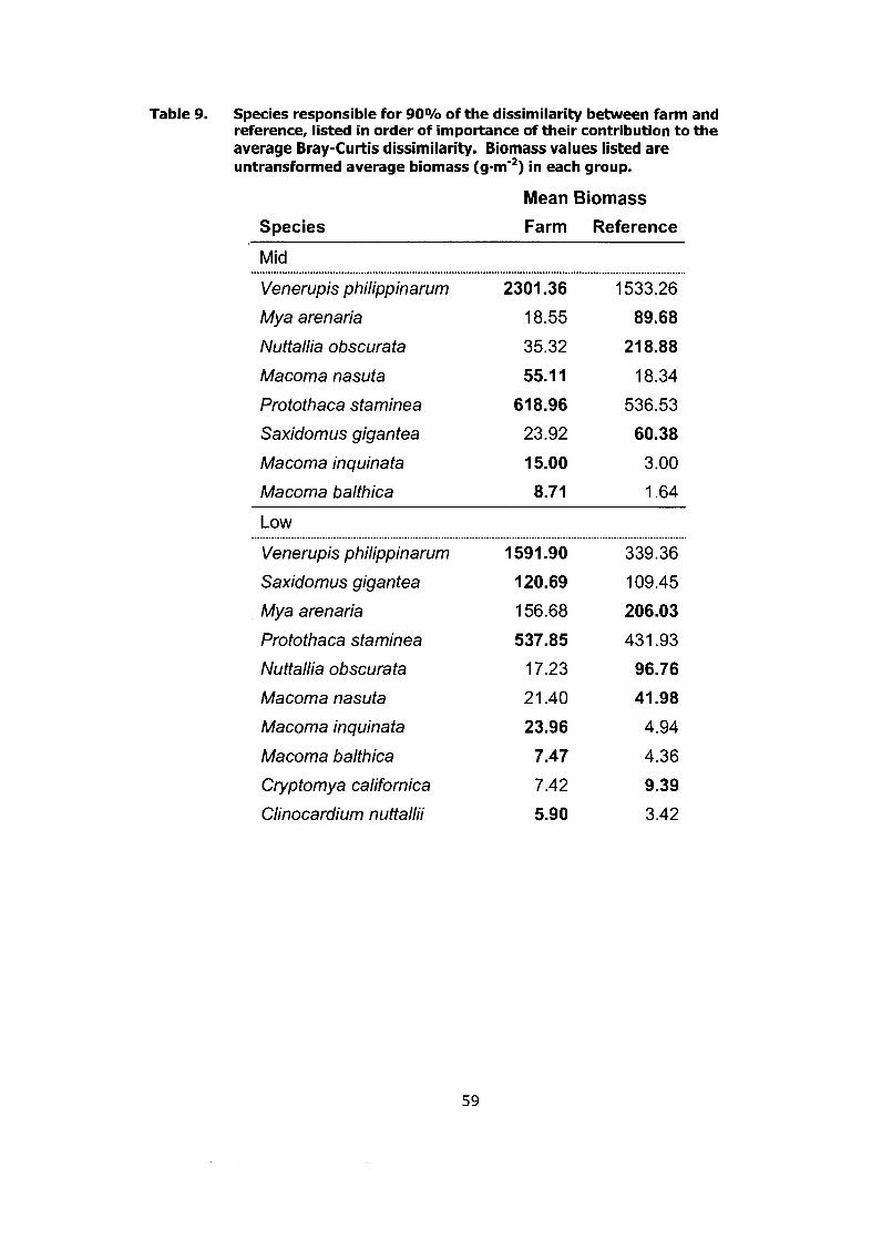
Table 9. Species responsible for 90% of the dissimilarity between farm and reference, listed in order of importance of their contribution to the average Bray-Curtis dissimilarity. Biomass values listed are untransformed average biomass (gsm-') in each group.
Mean Biomass
Species Farm Reference
Mid
Venerupis philippinarum
Mya arenaria
Nuttallia obscurata
Macoma nasuta
Protothaca staminea
Saxidomus gigantea
Macoma inquinata
Macoma balthica
Low
Venerupis philippinarum
Saxidomus gigantea
Mya arenaria
Protothaca staminea
Nuttallia obscurata
Macoma nasuta
Macoma inquinata
Macoma balthica
Cryptomya californica
Clinocardium nuttallii
3.2 Netting Experiment
3.2.1 Density
Faunal densities appear to vary little through time, and no decrease was
observed, even within control plots where depletion was expected due to
predation (see Figure 8). Repeated measures analysis of paired differences
found that the addition of the netting treatment after the baseline sampling
period had no effect on the difference in densities between netted and paired
control plots (see Table 10). There was also no significant interaction between
time and stratum on the paired differences in density for any faunal grouping
considered.

Figure 8. Mean Density (~nividuals-me') of fauna at each plot for time 0, 1 and 2. Values for netted plots are shown in black circles connected by a black line. Control means are plotted in open circles connected by a grey line. Error bars represent individual 95% confidence intervals for treatment means of plot values.
'0•‹ ] Predatory Infauna 300
200 / Bivalves (infaunal)
Time (sampling period)
1 Epifauna (non-net)
Venerupis philippinarum 300
'0•‹
1
200 - Other Infauna
150 -
100 -
Time (sampling period)
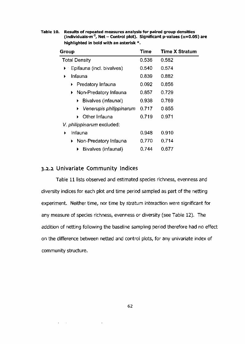
Table 10. Results of repeated measures analysis for paired group densities (individuals-m-2, Net - Control plot). Significant p-values (a=0.05) are
highlighted in bold with an asterisk *. Group Time Time X Stratum
Total Density
b Epifauna (incl. bivalves)
b lnfauna
b Predatory lnfauna
b Non-Predatory lnfauna
b Bivalves (infaunal)
b Venerupis philippinarum
b Other lnfauna
V. philippinarum excluded:
b lnfauna
b Non-Predatory lnfauna
b Bivalves (infaunal)
3.2.2 Univariate Community Indices
Table 11 lists observed and estimated species richness, evenness and
diversity indices for each plot and time period sampled as part of the netting
experiment. Neither time, nor time by stratum interaction were significant for
any measure of species richness, evenness or diversity (see Table 12). The
addition of netting following the baseline sampling period therefore had no effect
on the difference between netted and control plots, for any univariate index of
community structure.
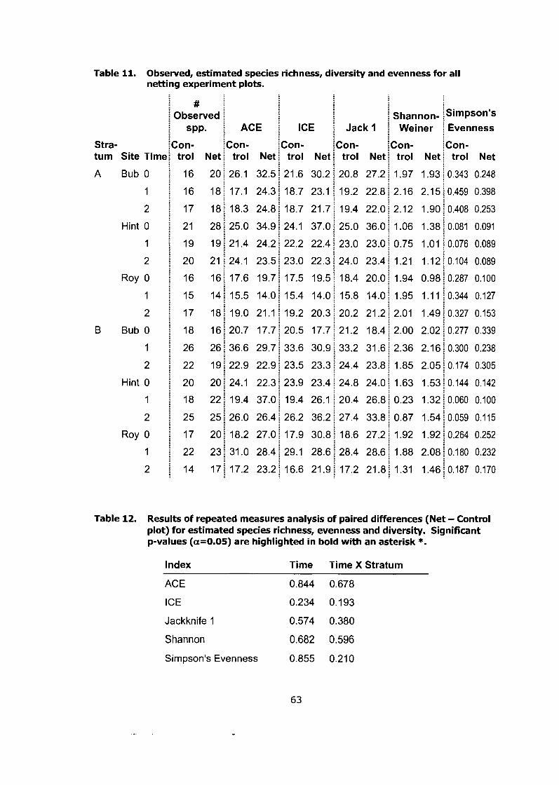
Table 11. Observed, estimated species richness, diversity and evenness for all netting experiment plots.
Stra- tum Site Time
A Bub 0
1
2
Hint 0
1
2
Roy 0
1
2
B Bub 0
1
2
Hint 0
1
2
Roy 0
1
2
# Observed
SPP.
:on- trol Net
16 20
16 18
17 18
21 28
19 19
20 21
16 16
15 14
17 18
18 16
26 26
22 19
20 20
18 22
25 25
17 20
22 23
14 17
ACE
Son- trol Net
26.1 32.5
17.1 24.3
18.3 24.8
25.0 34.9
21.4 24.2
24.1 23.5
17.6 19.7
15.5 14.0
19.0 21.1
20.7 17.7
36.6 29.7
22.9 22.9
24.1 22.3
19.4 37.0
26.0 26.4
18.2 27.0
31.0 28.4
17.2 23.2
ICE
:on- trol Net
21.6 30.2
18.7 23.1
18.7 21.7
24.1 37.0
22.2 22.4
23.0 22.3
17.5 19.5
15.4 14.0
19.2 20.3
20.5 17.7
33.6 30.9
23.5 23.3
23.9 23.4
19.4 26.1
26.2 36.2
17.9 30.8
29.1 28.6
16.6 21.9
Jack 1
Son- trol Net
20.8 27.2
19.2 22.8
19.4 22.0
25.0 36.0
23.0 23.0
24.0 23.4
18.4 20.0
15.8 14.0
20.2 21.2
21.2 18.4
33.2 31.6
24.4 23.8
24.8 24.0
20.4 26.8
27.4 33.8
18.6 27.2
28.4 28.6
17.2 21.8
Shannon- Weiner
:on- trol Net
1.97 1.93
2.16 2.15
2.12 1.90
1.06 1.38
0.75 1.01
1.21 1.12
1.94 0.98
1.95 1.11
2.01 1.49
2.00 2.02
2.36 2.16
1.85 2.05
1.63 1.53
0.23 1.32
0.87 1.54
1.92 1.92
1.88 2.08
1.31 1.46
Simpson's
Evenness
Son- trol Net
0.343 0.248
0.459 0.398
0.408 0.253
0.081 0.091
0.076 0.089
0.104 0.089
0.287 0.100
0.344 0.127
0.327 0.153
0.277 0.339
0.300 0.238
0.174 0.305
0.144 0.142
0.060 0.100
0.059 0.1 15
0.264 0.252
0.180 0.232
0.187 0.170
Table 12. Results of repeated measures analysis of paired differences (Net - Control plot) for estimated species richness, evenness and diversity. Significant p-values (a=0.05) are highlighted in bold with an asterisk *.
Index Time Time X Stratum
ACE 0.844 0.678
ICE 0.234 0.193
Jackknife 1 0.574 0.380
Shannon 0.682 0.596
Simpson's Evenness 0.855 0.210
3.2.3 Multivariate Analysis
MDS plots for each sampling period show no clear segregation of
treatments at any time, although plots from the same site do appear closer
together, at all time periods (see Figure 9). Two-way crossed ANOSIM tests for
difference between treatment levels and tide height stratum found no significant
differences at any time period (see Table 13). Small sample sizes only permitted
100 randomizations for each of these tests.
When plots from all time periods are shown together on a single MDS
plot, the lack of separation between netted and control plots becomes more
evident (see Figure 10). ANOSIM tests of differences between time periods, for
net and control groups separately, show no significant temporal differences
whatsoever (see Table 14). Sites are more strongly grouped overall by stratum,
or by site (see Table 15). Therefore, changes in community structure through
time, with the addition of netting for a period of 10 months, are insignificant
relative to differences between tide heights, or sampling sites.
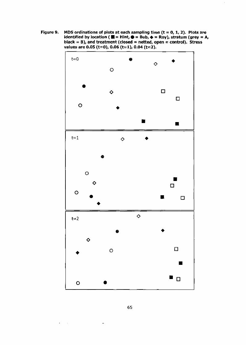
Figure 9. MDS ordinations of plots at each sampling time (t = 0, 1, 2). Plots are identified by location ( H = Hint, = Bub, + = Roy), stratum (grey = A, black = B), and treatment (closed = netted, open = control). Stress values are 0.05 (t=O), 0.06 (t=l), 0.04 (t=2).
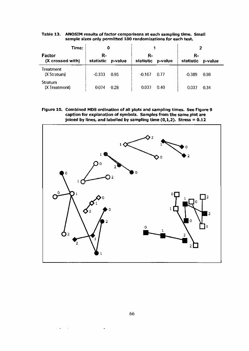
Table 13. ANOSIM results of factor comparisons at each sampling time. Small sample sizes only permitted 100 randomizations for each test.
Time: 0 1 2
Factor R- R- (X crossed with) statistic p-value I statistic p-value statistic p-value
Treatment (X Stratum)
Stratum (X Treatment)
Figure 10. Combined MDS ordination of all plots and sampling times. See Figure 9 caption for explanation of symbols. Samples from the same plot are joined by lines, and labelled by sampling time (0,1,2). Stress = 0.12
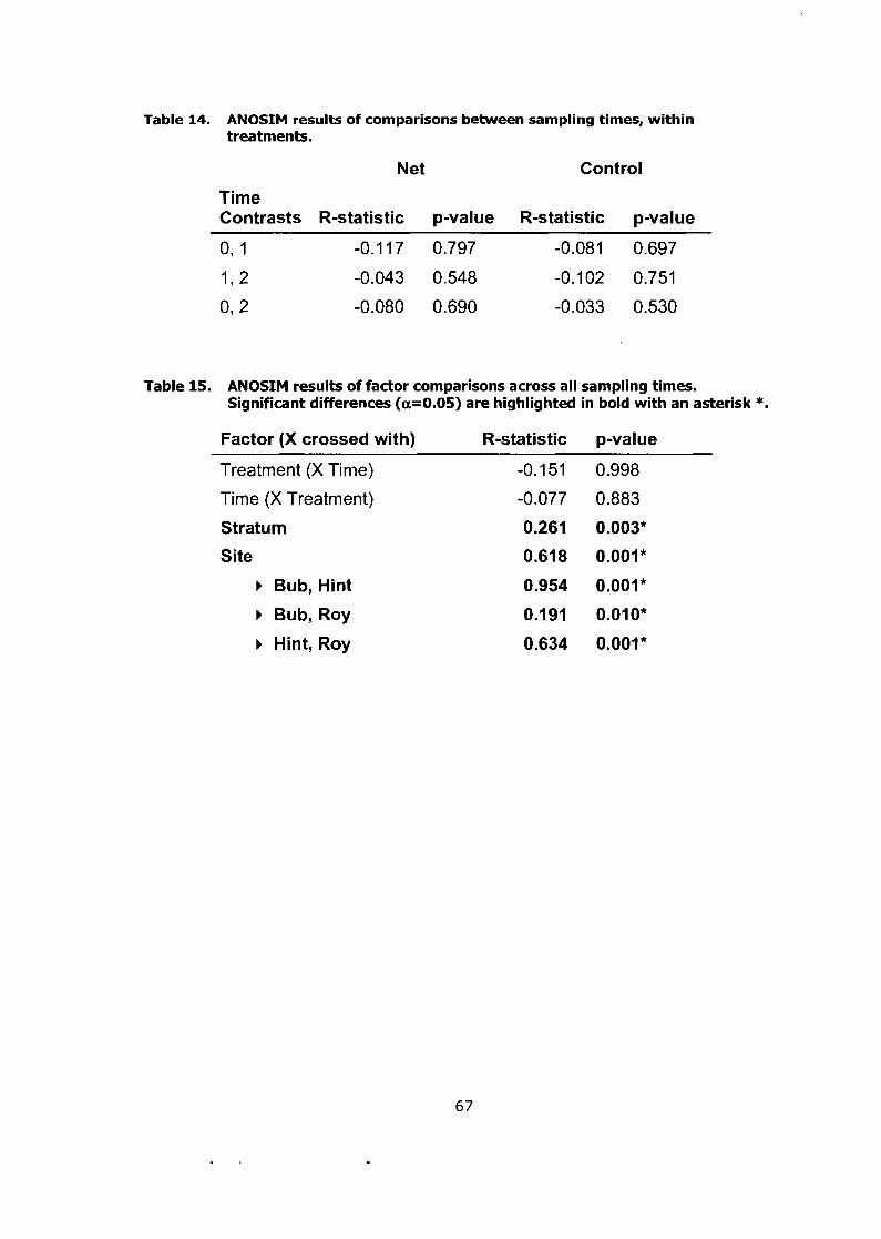
Table 14. ANOSIM results of comparisons between sampling times, within treatments.
Net Control
Time Contrasts R-statistic p-value R-statistic p-value
Table 15. ANOSIM results of factor comparisons across all sampling times. Significant differences (a=0.05) are highlighted in bold with an asterisk *.
Factor (X crossed with) R-statistic p-value
Treatment (X Time)
Time (X Treatment)
Stratum
Site
b Bub, Hint
b Bub, Roy
b Hint, Roy
Farm and reference sites differed very little in terms of most univariate
community indices (species richness, evenness, diversity), although multivariate
analyses showed subtle changes in variability. A small-scale netting experiment
found no general effects of netting, across a range of distinct sites. These
results highlight the difficulties of conducting research in intertidal soft-bottom
communities, where variability and relevant processes depend greatly on the
scale of measurement. Despite these challenges, analysis of species count data
can give useful information regarding possible impacts of shellfish aquaculture
practices, and lead to recommendations for maintaining the ecological
sustainability of this important industry.
Results of the field study provide insights into effects of two common
shellfish aquaculture practices operating together. The nature of the study does
not allow the separation of effects of netting and seeding practices common to
shellfish aquaculture. Nevertheless, these practices are used with the intention
of altering the ecology of these communities. Nets are used on clam tenures
with the intention of reducing predator pressure on commercial species, and
possibly other non-target species as an unintended result. The addition of clam
seed is intended to increase the productivity of the commercial species, which
can directly change the population dynamics of this species and possibly change
the strength and form of competition in intertidal communities. Therefore, the
results of this study must be considered within the context of predation and
competition and their role in structuring these communities.
The netting experiment was designed to assess the strength of predation
across different seasons, rather than directly addressing the effects of netting on
long-term community structure. The results of this experiment demonstrate that
short-term changes in community structure are unlikely to be affected by
netting, and that the temporal changes at a single site are much smaller than
differences between sites.
4.1 Netting and Predator Exclusion
Previous research in intertidal soft-bottom habitats suggests that large,
mobile epibenthic predators are often effective at limiting populations of

intertidal macroinvertebrates, including clams. I f netting used in clam
aquaculture reliably excludes such predators, then population densities are
expected to be higher in areas of netting, relative to unnetted reference sites, all
other factors being equal. The results presented in this work are not consistent
with such a prediction, indicating a lack of understanding of community dynamics
in this system, or invalid assumptions, or both.
Total bivalve density was found to be significantly higher in farm sites,
compared to unnetted and unseeded reference sites in the large scale field
study. This difference can be attributed entirely to the significantly higher
densities of the commercial Venerupis philippinarum on farm sites. The fact that
this was the only species to show significantly higher densities suggests that
most, if not all, clam species were not affected by the presence of netting on the
farm sites. This raises the question of what the effects are of intertidal netting
on clam farms.
4.1 .I Why only Venerupis philippinarum?
There are many possible explanations for why V. philippinarum was the
only species present in higher densities on farm sites. Clam aquaculture
practices may act to maintain a biophysical environment that truly only favours
this commercial species. While this might be the intent of aquaculture practices,
it seems unlikely that no other species would benefit incidentally.

Intertidal netting used in clam aquaculture may only prevent predation on
V. philippinarum, and allow other species to be regulated by the same forces
acting on the reference sites in this study. This could only be the case if V.
philippinarum were a preferred prey of a predator that was excluded by the nets.
The simplest explanation is that V. philippinarum is the only species added
as seed to the farm sites. The British Columbia Shellfish Grower's Association
(BCSGA) recommends adding Venerupis philippinarum seed at a density of 200
to 400 individuals per square metre, with an expected loss of 40-5O0/0 under
nets, before reaching harvest (BCSGA 2004b). This should account for a total
addition of 100-200 adult individuals of commercial size per square metre. The
sites used in this study are at various stages of harvest and seeding, but the
average increase in density is consistent with that expected due to seeding. On
the other hand, adult V. philippinarum are harvested after they are sexually
mature, allowing them to spawn for at least one season. The number of
individuals on farm sites resulting from natural spawning is unknown, which adds
uncertainty to the relative contribution of seeding to the observed differences.
Although V. philippinarum was the only bivalve species to show higher
densities and biomass on farm sites, total bivalve biomass did not increase
significantly. The abundance of other bivalves, excluding V. philippinarum, was
lower at farm sites on average, though not significantly different. The actual
difference may have been smaller than could be detected, due to large variation
in the data. Nevertheless, it stands to reason that if V. philippinarum is
increasing in abundance, yet total biomass is not significantly different, then
other species may be less abundant on sites exposed to common aquaculture
practices. This suggests that farm sites are dominated more by the commercial
species than paired reference sites, which is also supported by abundance data
at individual sites.
4.1.2 No Observed Effects of Predator Exclusion
The short-term netting experiment found no effect of netting on densities,
or community composition, over a 10-month period. However, the lack of a
decrease in densities in control plots also suggests that predation was not
affecting densities, and therefore there was no signal due to predation in the
data. Even when taking into account possible effects of infaunal predators, no
general pattern is apparent.
I t remains unclear why total bivalve densities, excluding V. philippinarum,
appear to be unaffected by netting in the field study. The fact that total
densities are similar between farm and reference sites suggests a few possible
explanations. I f netting excludes epibenthic predators, then predation may not
be limiting at these sites, and that other factors are preventing densities from
increasing in its absence. Even if netting provides a predator refuge, then space,
food availability, nutrients, or other unknown factors may prevent populations
from increasing above the current carrying capacity.
There is little evidence that space is a limiting resource in soft-bottom
sediments (Black and Peterson 1988, Peterson 1982, 1992), except perhaps for
large, deep-dwelling bivalves (Peterson and Andre 1980), which would have
been poorly represented in the sampling methods used in the present studies.
There is evidence, however, that food may be limiting in long, flat intertidal
areas, where a low rate of vertical mixing in the water column can allow filter-
feeding bivalves to deplete food particles at the sediment-water interface (Beal
et a/. 2001, Peterson 1992, Peterson and Black 1991). Experiments that have
observed possible food limitation in intertidal bivalves often infer such a
limitation from density-dependent growth. Density-dependent mortality has only
been attributed to food limitation in combination with environmental stress, but
may also be a result of predator responses.
Current research does not support the hypothesis that food limits
population sizes, but it can be a significant factor if it interacts with an additional
source of mortality, such as environmental stress, disturbance, or predation.
Bivalve densities, excluding the seeded V. philippinarum, ranged between
approximately 100 to 300 individuals m-2 at nearly all sites sampled, suggesting a
common upper limit to bivalve density. The notable exception to this pattern is
the D2 reference site, located near a public dock and within an area closed to
shellfish harvesting. The conditions at this site seem to support high densities
and biomass of all bivalve species, including V. philippinarum. The abundance of
bivalves at this site is greater than any other reference site, and exceeded only

by two farm sites, B l and Dl, which also have high densities of seeded V.
philippinarum.
There may also be a balance between the two forces of predator
exclusion, and other undocumented farming practices that favour a commercial
species over others. I f the nets act as a predator refuge, yet other farming
practices prevent populations of other bivalves from increasing, with the
exception of commercially favoured ones, that might explain the observed
patterns in bivalve density between farmed and reference sites. More
information about impacts of individual farming practices would help to separate
and explain the processes underlying these observations.
Many of the above-mentioned explanations and mechanisms affecting
total bivalve density are unlikely to affect all bivalve species in the same way.
The limitation of suspended food particles is not likely to limit the growth of
deposit-feeders, and selective predators may only limit populations of some
bivalve species and not others. Nevertheless, no consistent difference was
observed in bivalve biomass, densities or community composition, suggesting
that farm sites and reference sites are not fundamentally different in terms of
resource limitation. Despite similar densities, bivalve communities are subject to
different pressures on farm and references sites, particularly in the case of
farming practices and harvesting rates. There remains the question of how
predation on the bivalve community differs as a result of these farming practices.
4.1.3 Which Predators?
An alternate explanation for the results of this study is that the nets, as
used in B.C., do not effectively exclude epibenthic predators. Predators in the
water column may be able to get under the nets when they are submerged by
the tides, because some nets float and the edges are rarely buried, or secured to
the ground only at large intervals relative to the size of the predators. I n the
course of our sampling, we occasionally found fish or crabs trapped under nets
after the tide had receded. I n addition, many predators of benthic infauna are
themselves in ha bitants of the sediment (Ambrose 1984), and cannot be excluded
by surface netting. Infaunal predators tend to be smaller and are generally
thought to have a relatively minor, though constant effect on population sizes of
prey in soft- bottom sediments (Reise 1985). Infauna l predators may even
benefit from the exclusion of epibenthic predators, leading to a shift in predator
pressure on the benthic community (Gee et a/. 1985).
The aperture sizes of nets used in B.C. also would not exclude numerous
juvenile and small predators that can have seasonal effects on intertidal
populations. I f present at appropriate times of the year, these small predators
can affect bivalve populations by removing juveniles before they can achieve a
large enough size to be unmanageable by small predators (Reise 1985). The only
predator reliably excluded may be large diving ducks, which are thought to be a
major predator of clams (Jamieson et a/. 2001), and possibly poachers, whose
impacts are unknown.
4.1.4 Where have all the clams gone?
While evidence supports the hypothesis that scoters may be responsible
for the majority of clam disappearance at some sites (Lewis, unpublished data),
very little is still known about how scoter predation is affected by nets, or the
fate of bivalves that disappear from under protective netting. The BCSGA
(2004 b) expects that as many as 40 - 50% of seeded Venerupis philippinarum
clams are lost from under nets at a typical clam farm before reaching harvest.
Nevertheless, it is unknown whether these clams are consumed by predators, let
alone which predators, or if these clams simply migrate out from under the nets
to other areas.
Several clam farmers have described seeing clams crawl along the beach
surface, under nets, as well as trails left by clams moving within a site. Small
juvenile bivalves and gastropods are also able to spin mucous threads that allow
them to be pulled by water currents and wave action. This kind of
postmetamorphic drifting has been hypothesized to be an effective and
important mechanism of dispersal in some species, particularly those lacking a
highly mobile planktonic larval stage (Martel and Chia 1991). The ability of
Venerupis philippinarum to migrate in this manner is poorly understood, although
juveniles of the species have been observed to have moved following periods of
strong currents and wave action at some sites (Ydenberg, personal
communication). A better understanding of the vertical and horizontal dispersal
abilities of juvenile and adult V. philippinarum would allow more accurate
explanations of changes in populations sizes and densities, and bears more
detailed study.
The largest unknown factor affecting clam loss or mortality at all sites is
the illegal poaching of bivalves for commercial sale. Unprotected sites are more
susceptible to poaching, particularly during nighttime low tides in the winter, or
remote areas that are infrequently monitored, where poachers are less likely to
be observed.
4.1.5 Zonation
Biological interactions, such as predation and competition can play an
important role in determining the spatial distribution of intertidal benthic
macrofauna. The upper distribution of species is often limited by tolerance to
environmental extremes, such as desiccation with receding tide, larger variations
in temperature and salinity over short periods of time also associated with tidal
water movements, and also changes in sediment type that may occur over a tidal
gradient (Dame 1996). Lower intertidal limits of species, on the other hand,
appear to be the result of biological interactions including predation and possibly
competition (Paine 1974, Peterson 1992, Posey 1986).
Competition between Venerupis philippinarum and Nuttallia obscurata was
thought to account for the difference in distributions: N. obscurata is more
commonly found higher in the intertidal than V. philippinarum. I n the sites
sampled in the field study, however, N. obscurata was found even in low
intertidal areas, although at densities slightly lower on farm sites than reference
sites. Although the thinner shells of N. obscurata might make them more
appealing as a prey item, the lower biomass per clam compared to V.
philippinarum may render them energetically less favourable. N. obscurata also
has several adaptations which allow them to survive deeper in the sediment than
V. philippinarum (Gillespie et a/. 1999), thus avoiding predation and variable
environmental conditions at the surface.
There is a trade-off associated with living in intertidal areas. Greater
desiccation time in high intertidal areas not only reduces feeding time, but the
large fluctuations in environmental conditions can also be physiologically stressful
to benthic infauna. This stress can lead to even higher metabolic costs and a
non-linear decrease in growth and productivity (Beal etal. 2001). Although
environmental conditions are less stressful, and food more plentiful in lower
intertidal areas, infauna must also face more intense predation. Both epifaunal
and infaunal predators are more abundant lower in the intertidal (Ambrose 1991,
Beal et a/. 2001, Peitso et a/. 1994), which may explain why residents of these
areas tend to be species with adaptations to avoid predators, or to increase
handling time to the point of being energetically prohibitive (Kabat 1990,
Peterson 1982, Seitz etal. 2001). Species found higher in the intertidal may be
better adapted to surviving the stresses of exposure than predation.
Size-specific predation, in combination with a predation gradient can also
generate size gradients in benthic infauna, such as bivalves, with prey size
increasing or decreasing with distance from the low tide mark (Ambrose 1991,
Peitso eta/. 1994). I n the absence of predation, otherwise competitively
dominant species can also expand their distributions lower into the intertidal,
where they benefit from better growing conditions within a predator refuge
(Paine 1974, Posey 1986). Given the generally weak interspecific competition
observed in soft-bottom systems, such changes in distribution are not expected
to cause dramatic changes in other species, although dominance, and overall
biomass of a community may change in a simple additive manner. The
increased complexity of trophic structures in low intertidal areas means that
predation probably plays a much more important role in structuring communities
in this zone.
Tidal elevation was found to be a significant factor explaining changes in
community structure in the netting experiment, though not in the field study.
The low contrast between "low" and "mid" intertidal strata in the study may have
blurred the differences somewhat. Nevertheless, the difference in V.
philippinarum density between farm and reference sites was most significant in
the low stratum. Any predator-exclusion abilities of netting may be more
pronounced in the lower intertidal, where predation is also more intense.
4.2 Physical Changes of Predator Exclusion Structures
Many researchers (Kaiser et a/. 1996, Peterson and Beal 1989, Spencer et
a/. 1998) have suggested that nets, cages and other physical structures, used to
exclude predators in many studies, induce other changes, such as increased
sedimentation and food availability, that are independent of predator exclusion
and thus constitute an experimental artefact. Conclusions from such studies
should be considered in this light, and artefacts controlled for if at all possible.
I n the case of netting used by clam farmers, Spencer et a/. (1997) found
that changes in benthic community structure most likely occurred because of
changes in the physical characteristics of sediment, rather than the exclusion of
predators. Clam netting was shown to increase sedimentation rates, leading to a
concomitant increase in the a bundance of deposit feeding fauna (Kaiser et a/.
1996, Spencer etal. 1997). Increased sedimentation is often attributed to
physical structures used to exclude predators from soft-bottom marine
sediments, and can thus be confounded with the desired exclusion of predators
(Gee etal. 1985). This artefact of experimental manipulation does not seem to
be as much of a problem for experiments in rocky substrata.
Predator-exclusion structures can baffle waves, moderate disturbance
(Gee et a/. 1985, Peterson 1984, Reise 1985, Spencer et a/. 1997), and also act
as attachment structures for macroalgae, which can further reduce water
velocities and increase the deposition of organic particles to the sediment
surface. I n the aquaculture industry, these and associated organisms are
referred to as "bio-fouling" and are removed regularly to allow water circulation
through the nets, and prevent potentially adverse chemical conditions that may
occur beneath decomposing carpets of macroalgae.
Physical effects of clam netting were not analyzed in the present study.
Possible differences between farm and reference sites were controlled for, but if
clam aquaculture practices altered the physical conditions of farm sites from their
pre-farm state, this study would not have been able to observe such an effect.
Thus, if farming practices altered the physical characteristics of the site, such
changes would have occurred prior to sampling, and the reference sites matched
to the current state, not the baseline pre-farm state of a farm site. This might
account for the overall similarity between farm and reference sites observed in
the study, since community structure is heavily influenced by the physical
properties of a site, including sediment particle size, exposure, currents, or
nutrient availability.
4.3 Change and Variability
Intertidal macroinvertebrate communities are recognized as being highly
variable communities in both space and time (Beal et a/. 2001). This variability
has posed a challenge to researchers, making it difficult to detect changes
amidst high levels of variation.
Results from the small-scale netting experiment found no difference
between treatment groups with respect to macrofaunal densities or community
composition. Examination of the data reveals that differences between sites,
which were the replicates in this experiment, were greater than differences
between treatments, or even tide height strata. MDS plots show that although
some degree of a serial shift in community structure through time was observed
at each site, differences between time periods remained smaller than average
differences between plots. It is possible that differences in the biophysical
environment between replicates were large enough to mask any effect of the
netting treatment in the multivariate context.
Further such experiments might yield more precise results by better
controlling for environmental variables such as sediment particle sizes, tidal
submersion, and other factors known to affect the species composition of
intertidal communities. Many other experiments that have demonstrated effects
of predator exclusion have succeeded in this regard, even when using plots
smaller than those in the present study, by replicating within a single site, rather
than across possibly different environmental conditions. The physical
environment may determine the relative importance of predation and
competition in structuring communities. Consistent effects of these biological
interactions may not have been observed in our results because of large
variations in environmental conditions, and therefore in the strength of predation
or competition, or both. Experiments at larger geographical scales are more
informative with regards to general impacts (Beal etal. 2001, Emmerson etal.
2001, Peterson 1992), but individual sites may respond independently, and this
must be taken into account.
I n the large scale field study of bivalve communities presented here, there
was no significant difference between farm and reference sites with respect to
univariate community indices, community composition, or macrofaunal densities,
excluding Venerupis philippinarum. Nevertheless, multivariate community
analysis revealed an apparent change in among-site variability in community
composition between treatment groups. Farm sites are slightly more similar to
each other, on average, than reference sites. This explains why the regional
separation evident among reference sites is not as noticeable among farm sites.
These results suggest that although farming practices do not consistently
alter community structure to a point that is outside the range observable among
reference sites, the farm sites do appear more similar to each other than is the
case with unfarmed sites. It is unknown if farm sites have changed from their
original pre-farm states, to their current state, which is not noticeably different
from existing reference sites. Unfortunately, the baseline data required to make
such an assessment is largely absent for many sites where shellfish aquaculture
is currently active.
The results of this study suggest that the two common practices of
seeding and netting are not associated with large, negative changes in bivalve
community structure at a site suitable for aquaculture. The loss of 'regional
distinctness' among farm sites appears to be primarily a result of increased
consistency in densities of common species at farm sites. Sites selected and
approved for clam farming may also represent a su b-set of possible community
types, which are common to all regions included in the study. I f this were the
case, then communities on pre-farm sites would be expected to be most similar
to existing farm sites than other reference sites. Although small sample sizes do
not permit a statistical test of this hypothesis, a cursory examination of the MDS
plots suggests this may not always be the case.
Sites may be affected to varying degrees by farming practices, but it is not
known what factors would mitigate such impacts. Depauperate areas, or those
exposed to intense predation or disturbance may benefit from the stabilizing
effects of netting. On the other hand, regionally representative, unique areas or
biodiversity "hotspots" may experience a loss in the abundance of some species
and a decrease in diversity as the moderating effects of aquaculture practices
lead to an increase in similarity with other farm sites that are dominated by
commercial species.
I f clam tenures become increasingly dominated by a single commercially
valuable species, what are the implications for ecosystem processes, such as
nutrient cycling, performed by bivalves? It has been argued that if many species
contribute to carry out activities such as filter-feeding, deposit-feeding,
burrowing, and nutrient cycling, this can reduce variability in functional
processes, as different species operate optimally under different environmental
conditions (Emmerson etal. 2001, McCann 2000, Yachi and Loreau 1999). I n
some cases, species-rich communities have been observed to.out-perform the
best monocultures in total productivity (Tilman et a/. 2001). On the other hand,
a single species may be all that is necessary in some situations to carry out a
particular ecosystem function (Worm and Duffy 2003). Species-rich assemblages
may simply have a greater chance of including a single, highly active species that
results in an overall high level of ecosystem function (Loreau 2000).
The conditions created by clam farming, which are intended to favour the
production of commercial species, may create common pressures that drive
separate communities toward higher levels of similarity. The homogenizing force
of clam farming at large scales appears to be more significant than potential
impacts at individual sites. The ability of common farming practices to alter
habitat heterogeneity at smaller scales was not documented in the present
study, but is deserving of further research. Nevertheless, the increased similarity
among farm sites suggests that impacts of clam farming may be more relevant
to larger scale processes.
4.4 Scale of changes
I n both the netting experiment and field study presented here, no
consistent differences were attributable to the treatments applied, yet there was
evidence of other factors operating at different scales than that of the
experimental units. I n the netting experiment, large-scale site and tide
differences overshadowed possible treatment differences, or even serial changes
through time. This might explain why no effect of predator exclusion was
observed in this experiment, in contrast to many other small-scale predator-
exclusion experiments.
Many published experiments using nets or cages to exclude predators
used plots in the range of 0.25 m2 to 10 m2 (Beal eta/ . 2001, Drake and Arias
1996, Reise 1985, Seitz et a/. 2001, Spencer eta/. 1996, 1997, 1998,
Summerson and Peterson 1984, Vargas 1988, Wiltse 1980), which is at least as
small as those used in the experiment presented here. Many of these studies did
find at least small effects of predator exclusion, including changes in density
(Beal et a/. 2001, Drake and Arias 1996, Reise 1985, Summerson and Peterson
1984), species richness (Spencer et a/. 1997, Wiltse 1980), or community
composition (Spencer et a/. 1996, Vargas 1988). Two important differences
between our netting experiment and the others might explain the disagreement
in results. First, this experiment included a much shorter time scale than most,
which did not allow for recruitment, or other multi-generational effects to be
observed. Second, most other experiments replicated plots within a single site,
or a relatively small geographic area, whereas the plots in the present
experiment were spread out over a much larger area. The latter difference
would account for the significant site differences, which are likely the result of
differences in sediment particle size, exposure, presence of large predator
populations, and other factors that significantly affect community structure.
The fact that macroinvertebrate densities did not decrease on control
plots suggests that even if predators were excluded by the experimental netting,
that the difference in predation rates between treatments may have been
insignificant. The size of the netting plots may have been too small to capture
effects of predators, if they forage at larger scales. Any differences in density
observed may be the result of migration in and out of the plots, or random
variation associated with different sampling points within plots. Future studies of
the effects of anti-predator netting might yield more informative results by better
controlling for confounding factors such as tidal elevation, sediment type,
predation intensity and also by including a broader temporal scale by conducting
such an experiment over several years.
Some of these considerations are accommodated by the large-scale field
study. Active clam farms show integrated changes over the entire length of the
tenure. While the spatial difference between a farm and reference site is
sometimes a poor surrogate for time, the costs in time and resources of such a
study make it more efficient than an experiment at the same scale. Results of
this field study show no noticeable differences between farm and reference sites
as a whole, but do indicate regional differences among reference sites, which are
noticeably smaller among farm sites. Once again, effects at different spatial
scales are evident in the data.
This is consistent with a growing body of theory regarding processes
affecting marine benthic ecology. Direct, exploitative competition may be
relatively unimportant in structuring marine soft-bottom communities (Black and
Peterson 1988, Peterson 1992). Habitat heterogeneity, caused by biotic or
abiotic processes, may act at the smallest scales, creating random patchiness
and variability within a community (Peterson 1984, Posey 1986, Seitz et al. 2001,
Summerson and Peterson 1984). Predation, as a top-down process, may be
most important and evident at intermediate scales, but nutrient dynamics and
other bottom-up limitations may dominate at larger scales (Posey etal. 2002).
Regional differences in the field study, and site differences in the netting
experiment are likely the result of differences in either bottom-up or top-down
effects. The challenge remains in determining which factor is most relevant, and
the absolute size of each scale. I n either case, predation does not appear to be
a limiting factor at any scale included in the research presented here.
The results of the field study indicate that farming practices, including
seeding and netting, may only affect communities at spatial scales larger than
even the largest single tenure included in the study. I f clam farming is a
homogenizing force at large scales, then the most important impact of clam
aquaculture would be as a result of smaller, cumulative impacts of several
tenures within a given geographical area. For example, if a species is not self-
sustaining on sites used for clam aquaculture, but maintained only by the
constant influx of larvae from other sites, then large-scale farming may have the
potential to affect meta-populations that are relatively unaffected by smaller
areas of aquaculture.
There remains a large level of uncertainty regarding impacts of individual
practices, or indeed the mechanisms underlying many of the results presented
here. Nevertheless, there are clear implications for the management of coastal
biological resources in British Columbia, Canada. Given the potential for
unknown, large-scale cumulative impacts and the possibility for site-specific
responses to farming practices, I would recommend that regulatory efforts focus
on baseline data-collection, monitoring and site-selection at the regional scale.
Specific areas of high biodiversity, or uncommon habitats that support
endemic species and communities, may be the most susceptible to negative
changes resulting from aquaculture activities. Such areas should be identified
and protected, in light of the uncertainty surrounding impacts of aquaculture
practices. The shellfish aquaculture industry has supported a provincially-
enforced standard code of practices to limit impacts at individual sites (BCSGA
2003), but only the government agencies responsible for site approvals are in a
position to adequately monitor and control how aquaculture is distributed within
regions. The results presented here suggest that this is the scale at which
impacts are most likely.
Cumulative impacts resulting from a homogenizing force of clam farming
could be most likely if sites are clustered closer together, leading to greater
effects to large-scale processes. A precautionary approach therefore suggests
spreading out aquaculture sites, rather than clustering several adjacent sites
within a single geographic area.
5.0 SUMMARY A N D
CONCLUSIONS
Shellfish aquaculture has the potential to grow into an economically
important industry in British Columbia, Canada. Nevertheless, very little is
known about the potential impacts to the environment or biotic resources,
particularly to non-target species, which share the same habitat and resources as
commercially important species. Research presented here has focused on the
common clam farming practices of seeding the intertidal with juvenile Venerupis
philippinarum, and covering these areas with protective netting.
The intent of the nets is often to exclude large, epibenthic predators,
which are believed to significantly deplete populations of commercially important
bivalve species, such as V. philippinarum. Recent studies of predator exclusion
in marine soft-bottom habitats have suggested that predation does not play a
major role in structuring communities, but it can limit prey population sizes.
Competition has also been infrequently considered an important
determinant of community structure in this environment, although it may lead to
patchiness within a community. Intraspecific competition appears to be stronger
in soft-bottom communities, primarily affecting growth rates of individuals, and
being more common in the presence of stressful abiotic conditions. Nutrient
dynamics and food availability have been found to be important at large regional
scales, but only occasionally seem to lead to significant intraspecific competition
at local scales. The most common factor affecting community structure in
marine soft-bottom habitats appears to be abiotic environmental conditions such
as sediment size, temperature, and desiccation determined by tidal elevation.
Factors such as competition and predation may only affect the tidal elevation or
spatial distribution of some populations, while being otherwise largely
insignificant to community structure at the local scale.
The results of both a small-scale netting experiment, and a large-scale
field study of clam tenures is consistent with these hypotheses. Very few
predicted results of predator exclusion were observed under netted areas, either
in terms of density, biomass, or community composition. This suggests that
either predation is not limiting at the sites sampled, or that the nets do not
effectively alter predator pressure. Most variation in the data could be explained
by tidal elevation, or even more importantly, by large-scale differences between
sites or regions, likely caused by differences in environmental conditions. This
also agrees with other studies of the effects of aquaculture netting, which found
changes in community structure attributable primarily to increased sedimentation
caused by the physical structure of the netting, rather than any effect of
predator exclusion.
There were few consistent differences in bivalve communities between
active clam tenures using seeding and netting, and paired reference sites.
Although there were few site-level differences, there was an increase in overall
similarity among farm sites, leading to a decrease in regional distinctness
otherwise evident among reference sites. The implications of increased similarity
between sites are of greatest concern to large-scale processes. If clam farming
sites become increasingly dominated by commercial species, there are also
implications for ecosystem functions, such as nutrient cycling.
The results also suggest that sites may respond differently to farming
practices, with some benefiting from increased structural heterogeneity, and
others losing endemic or rare species to the possible homogenizing effects of
aquaculture. This leads to the recommendation that the process of locating and
approving sites for clam aquaculture should consider sites in a regional context,
in addition to local site criteria. A precautionary approach suggests preventing
clam aquaculture sites from being too clustered, thereby limiting possible
unforeseen cumulative impacts.
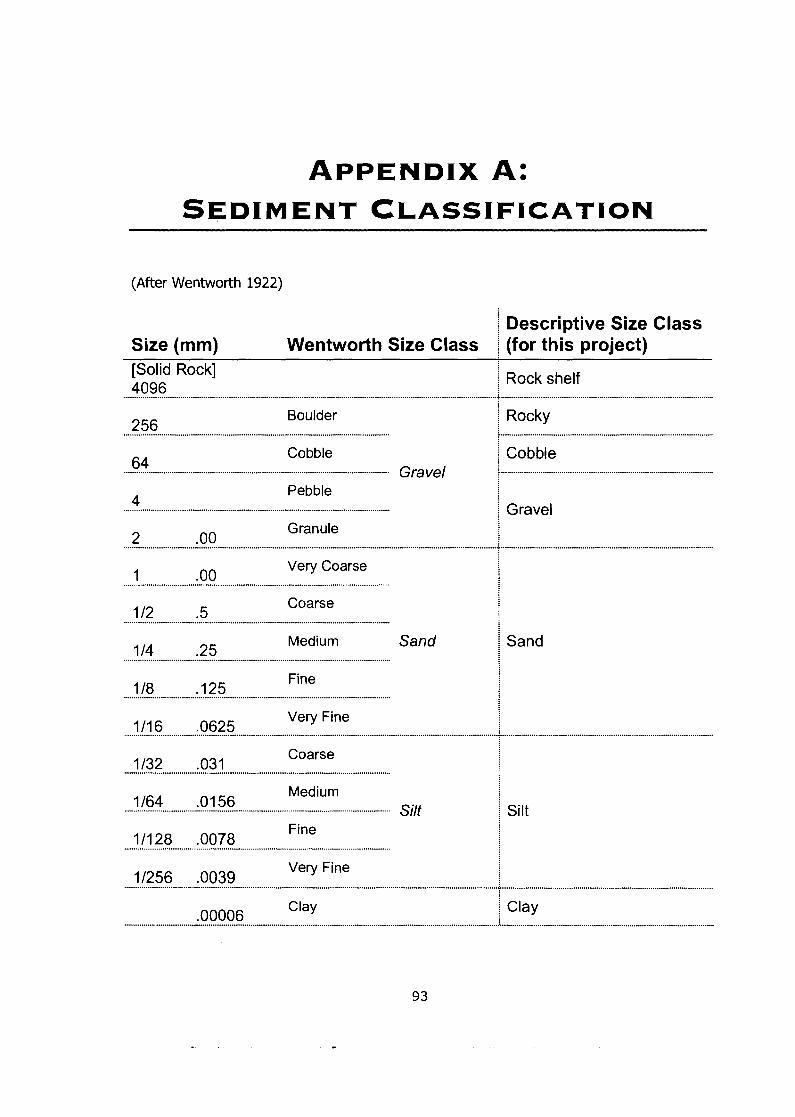
(After Wentworth 1922)
Size (mm) Wentworth Size Class [Solid Rock] 4096
256 Boulder
...........................................................................................................................................
64 Cobble
........................................................................................................................................... Gravel
4 Pebble
2 .oo Granule ..................................................................................................................................................................................................
1 .oo Very Coarse
Coarse
1 14 .25 Medium Sand
...........................................................................................................................................
1 I8 1 2 5 Fine
...........................................................................................................................................
Very Fine
1/32 .031 Coarse
...........................................................................................................................................
1164 .0156 Medium
........................................................................................................................................... Silt
11128 .0078 Fine
Very Fine
.00006 Clay
Descriptive Size Class (for this project)
Rock shelf
Rocky .............................................................................................................
Cobble
Gravel
.............................................................................................................
Sand
Silt
.............................................................................................................
Clay

After the first major field season in this project during the summer of
2003, the field sampling methods were re-examined in orderto increase the
speed and efficiency of data collection. The major limitation in collecting data for
this project was time.
Coastal British Columbia, Canada typically has one suitable tidal cycle with
the lowest low of the day, allowing 6 - 10 hours exposure for areas below 2 m
above chart datum, which is the upper limit of the "low" strata used in this
research. I n addition, the summer field season only allows a limited number of
days with tides low enough to allow such sampling, usually 10 days of every 2
week period. Because tidal cycles themselves oscillate over this time, the lowest
tides, and longest sampling days, are in the middle of this 10 day period, while
the first and last are the shortest sampling days.
As a consequence of these time constraints, there are a maximal number
of quadrats that can be sampled in the season, and the only way to increase this
number is to reduce the amount of time required for each quadrat. Although
sample sizes seemed to be adequate at each site, no new sites were expected to
be included in subsequent sampling efforts, and so to increase power it was
deemed that increasing sampling effort at existing sites would increase precision
at each site, and hopefully reduce unexplained variation. The sampling
procedure described in the Methods section of this work (see above) was
intended to capture as much information as possible, but a desire to reduce the
time per sample led to a re-examination of the benefits, in terms of information
content, of the smaller sieve. Experience in the field indicated that material from
a smaller (0.25 x 0.25 m) quadrat sifted through a 1 mm sieve required as much
time to process as material in the larger quadrat (0.5 x 0.5 m), sifted through a 6
mm mesh sieve. Time data is not available for each sieve size, but this
generality is based on personal experience, and the fact that the 1 mm mesh
sieve allows very little sediment to pass through, leaving a large proportion to
sift through by hand to locate and count macrofauna, even after pre-sieving with
a 6 mm mesh.
Methods & Analysis
Results presented here include data from 28 sites sampled (14 pairs) in
mid and low intertidal areas, from 3 regions in B.C.: Barkley Sound, Baynes
Sound, and Okeover Inlet in Desolation Sound. Most sites were sampled with 18
quadrats, although some included only 12 quadrats (see Methods, above for
details on sample sizes and site characteristics). All observed macrofaunal
species were included in the analysis of the effect of mesh size on results.
It is important to note in the results that counts from the small sieve
include only those individuals retained by a 1 mm mesh, and not those retained
by the 6 mm mesh. Counts from the large sieve include all individuals retained
by a 6 mm mesh, including those from within the subsample that was also sieved
through a 1 mm mesh afterward. Because the small quadrat (0.25 m x 0.25 m)
was used to sample sediment for the smaller sieve, counts (# individuals) are
normalized to the same area as the large quadrat, usually by converting both to
individualsmm-2. Occasionally, some abundant surface individuals were recorded
only in the small quadrat, to help speed up data collection, and some counts may
have been accidentally recorded in the incorrect list by field assistants, but this is
assumed to be negligible. I f anything, it would mean that the number of
individuals and species in the small sieve reported here are slightly
overestimated.
Mean densities per site were calculated using all quadrat samples at each
site. The number of species observed was noted for pooled quadrats at each
site, and as a mean per quadrat at each site. Means of each of these values
over all sites were plotted on graphs, although to calculate statistical
significance, the difference between large and small sieve values at each site
were analyzed as a paired t-test.
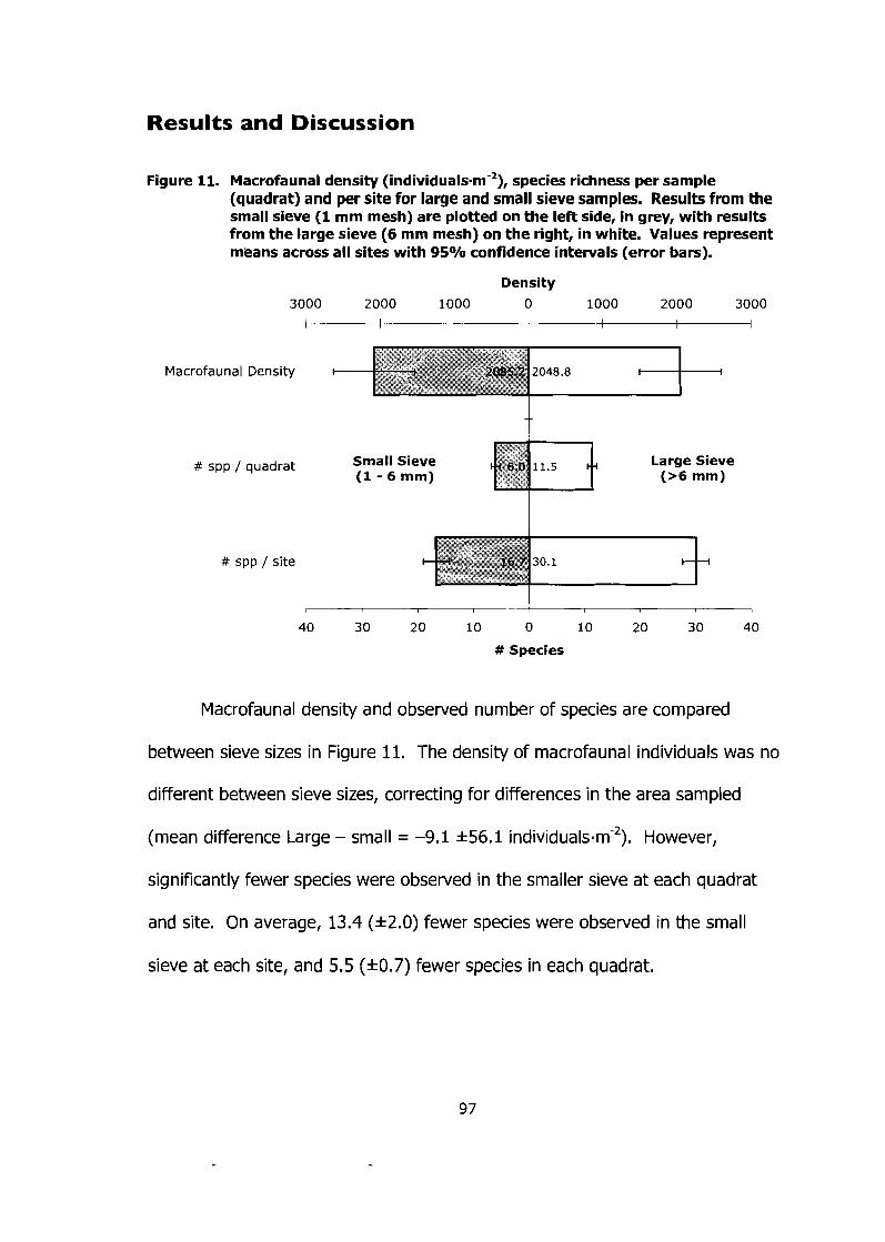
R e s u l t s and Discuss ion
Figure 11. Macrofaunal density (individua~s.rn~~), species richness per sample (quadrat) and per site for large and small sieve samples. Results from the small sieve (1 mm mesh) are plotted on the left side, in grey, with results from the large sieve (6 mm mesh) on the right, in white. Values represent means across all sites with 95% confidence intervals (error bars).
Density 3000 2000 1000 0 1000 2000 3000
# spp / quadrat Small Sieve Large Sieve ( 1 - 6 mm) (>6 mm)
# spp / site
I I , I I I I I I
40 3 0 20 10 0 10 20 3 0 4 0
# Species
Macrofaunal density and observed number of species are compared
between sieve sizes in Figure 11. The density of macrofaunal individuals was no
different between sieve sizes, correcting for differences in the area sampled
(mean difference Large - small = -9.1 k56.1 individ~als.m-~). However,
significantly fewer species were observed in the smaller sieve at each quadrat
and site. On average, 13.4 (k2.0) fewer species were observed in the small
sieve at each site, and 5.5 (k0.7) fewer species in each quadrat.
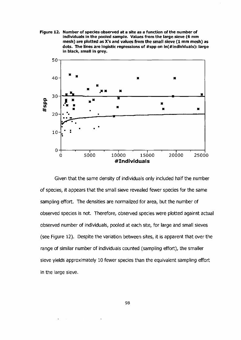
Figure 12. Number of species observed at a site as a function of the number of individuals in the pooled sample. Values from the large sieve (6 mm mesh) are plotted as X's and values from the small sieve (1 mm mesh) as dots. The lines are logistic regressions of #spp on In(#individuals): large in black, small in grey.
Given that the same density of individuals only included half the number
of species, it appears that the small sieve revealed fewer species for the same
sampling effort. The densities are normalized for area, but the number of
observed species is not. Therefore, observed species were plotted against actual
observed number of individuals, pooled at each site, for large and small sieves
(see Figure 12). Despite the variation between sites, it is apparent that over the
range of similar number of individuals counted (sampling effort), the smaller
sieve yields approximately 10 fewer species than the equivalent sampling effort
in the large sieve.
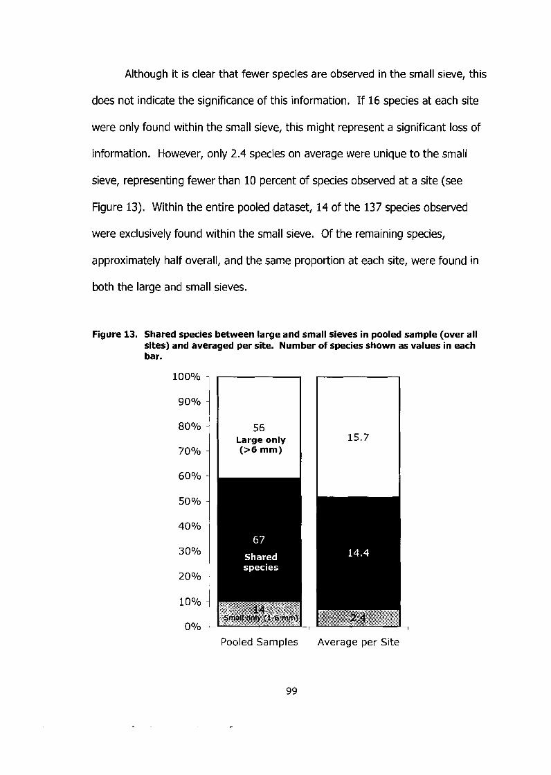
Although it is clear that fewer species are observed in the small sieve, this
does not indicate the significance of this information. If 16 species at each site
were only found within the small sieve, this might represent a significant loss of
information. However, only 2.4 species on average were unique to the small
sieve, representing fewer than 10 percent of species observed at a site (see
Figure 13). Within the entire pooled dataset, 14 of the 137 species observed
were exclusively found within the small sieve. Of the remaining species,
approximately half overall, and the same proportion at each site, were found in
both the large and small sieves.
Figure 13. Shared species between large and small sieves in pooled sample (over all sites) and averaged per site. Number of species shown as values in each bar.
l ooO/o
9 0 O/o
8 0 O/o
7 0 O/o
6 0 O/o
5 0 O/o
4 0 O/o
3 0 O/o
2 0 O/o
1 0 O/o
0 O/o
Large only (>6 mm)
Pooled Samples Average per Site
9 9
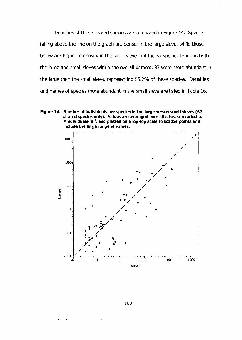
Densities of these shared species are compared in Figure 14. Species
falling above the line on the graph are denser in the large sieve, while those
below are higher in density in the small sieve. Of the 67 species found in both
the large and small sieves within the overall dataset, 37 were more abundant in
the large than the small sieve, representing 55.2O/0 of these species. Densities
and names of species more abundant in the small sieve are listed in Table 16.
Figure 14. Number of individuals per species in the large versus small sieves (67 shared species only). Values are averaged over all sites, converted to #individ~als.m-~, and plotted on a log-log scale to scatter points and include the large range of values.
small
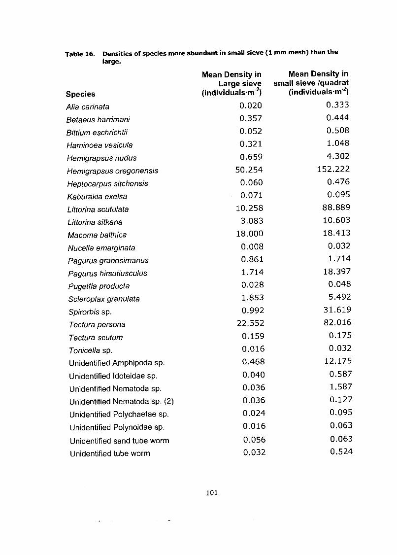
Table 16. Densities of species more abundant in small sieve (1 mm mesh) than the large.
Species
Alia carinata
Betaeus harrimani
Bittium eschrichtii
Haminoea vesicula
Hemigrapsus nudus
Hemigrapsus oregonensis
Heptocarpus sitchensis
Kaburakia exelsa
Littorina scutulata
Littorina sitkana
Macoma balthica
Nucella emarginata
Pagurus granosimanus
Pagurus hirsutiusculus
Pugettia producta
Scleroplax granulata
Spirorbis sp.
Tectura persona
Tectura scutum
Tonicella sp.
Unidentified Amphipoda sp.
Unidentified ldoteidae sp.
Unidentified Nematoda sp.
Unidentified Nematoda sp. (2)
Unidentified Polychaetae sp.
Unidentified Polynoidae sp.
Unidentified sand tube worm
Unidentified tube worm
Mean Density in Large sieve
(individual~~m'~)
0.020
0.357
0.052
0.321
0.659
50.254
0.060
0.071
10.258
3.083
18.000
0.008
0.86 1
1.714
0.028
1.853
0.992
22.552
0.159
0.0 16
0.468
0.040
0.036
0.036
0.024
0.016
Mean Density in small sieve /quadrat
(individuals-m'*)
0.333
0.444
0.508
1.048
4.302
152.222
0.476
0.095
88.889
10.603
18.413
0.032
1.714
18.397
0.048
5.492
31.619
82.016
0.175
0.032
12.175
0.587
1.587
0.127
0.095
0.063
0.063
0.524
Species observed exclusively in small sieve:
Balanus balanoides
Caridae sp.
Chthamalus dalli
Nutricola tantilla
Tellina modesta
Unidentified Annelida sp.
Unidentified Bivalve spp.
Unidentified clam sp.
Unidentified Nematoda sp. (3)
Unidentified Nematoda sp. (yellow)
Unidentified worm sp.
Unidentified worm (b)
Unidentified worm (c)
Unidentified worm (s)
Conclusion
I f a bout half of all observed species are common to both sieves, and half
of those shared species are more abundant in the large sieve, then the large
sieve includes a significant sample of over three-quarters of the species sampled.
By using only a 6 mm mesh and not a 1 mm mesh sieve, fewer than 10% of the
species would not be counted, and only 25% of those observed would be under-
represented. Considering the equal time required and the lower information
content, the small sieve appears to be much less efficient than the larger one, at
least in terms of information gain per unit sampling effort and time. I propose
that the increased precision achievable with more samples at each site using only
the large sieve can be more useful than more detailed information with fewer
samples, using a 1 mm mesh sieve.
Included here are the raw data matrices used in the multivariate
community analyses. Replicates (sites) are listed as rows and species as
columns. Table 17 shows average density per square metre (# individuals~m-2,
for infaunal bivalves species in the field study. Table 18 shows biomass data for
the same species, in total g-m-2. Because biomass data was collected at only
one of every three quadrats sampled for count data, not all species in the density
data are represented in the biomass data. Sites in both these matrices are
labelled as follows: The first letter indicates the region (A = Baynes, B = Barkley,
D = Desolation), this is followed by a sequential number to identify each site
within the region, a lower-case letter indicates the tide height stratum of the site
(I = low, m = mid), and the final digit indicates the treatment group of the site
(1 = farm, 0 = reference). For example, Al l1 is a site in Baynes Sound (Al), in
the low stratum, and is a farm site.
Table 19 presents pooled count data from the small-scale netting
experiment, where each value is a total of counts in each plot. Because sample
sizes were equal across all plots, there was no need to correct for differences in
sampling intensity. These values may be converted to mean density by dividing
by the number of quadrats per plot (5) and scaling up to 1 m2 (x4): multiply
each value by 0.8 (4/5). Plots in the netting experiment are labelled with an
abbreviated location name (Bub, Hin, Roy), followed by a dash, then the tide
stratum identifier (A or B), treatment (1 = net, 0 = control), and another dash
separates the sampling period of the sample (0, 1, 2). For example, Bub-AO-0 is
site Bub, stratum 'A' control plot at time 0 (baseline data).
Species that were omitted from the multivariate analysis are included
here, but their names are highlighted in bold.
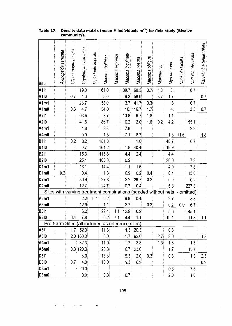
rable 17. Density data matrix (mean # individuals-m-') for field study (Bivalve
Site
community).
Sites with varying treatment combinations (seeded without nets - omitted): 1 43ml : 2.2 0,4/ 0.2 9 . 8; . 0 . 4: . : 2 . : 71 1 3.8 1 I : 43m0 12.9 1 1 , . : / 2.7' 0.21 0.2, 0.9 6.7' 1 1
3311 1 ! 6.2 B310 0.4 7.8
I
22.4 1.11 12.9 0.2: i 5.6; / 45.1. 6.2. 7 .1 4.4 1.1, , 19.1: 1 . 8 1.1
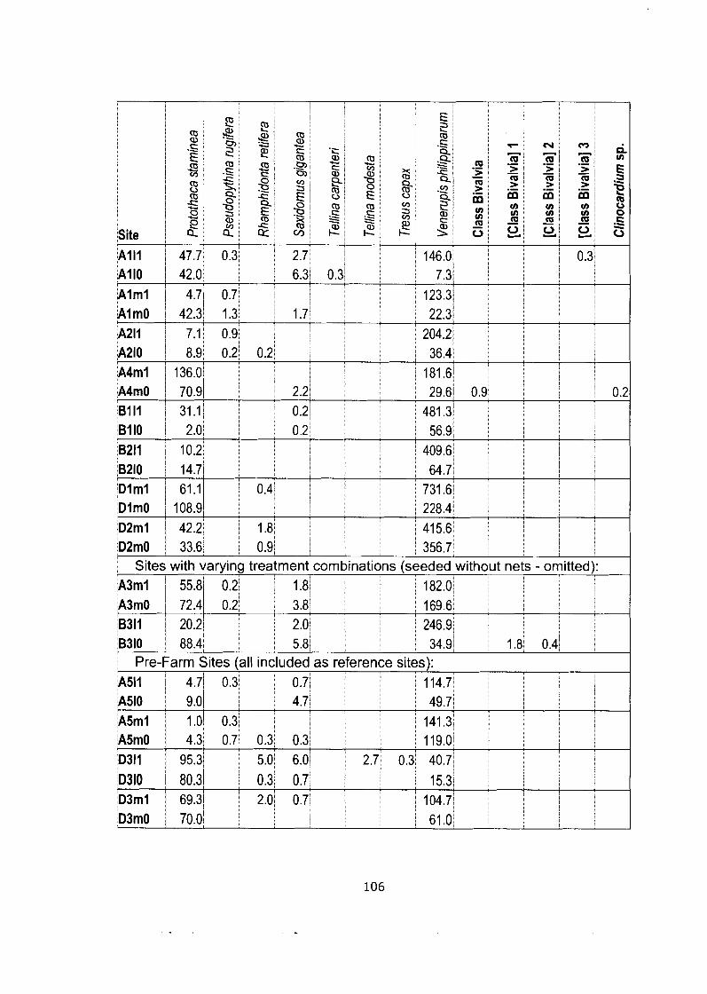
Sites with varying treatment combinations (seeded without nets - omitted): ~ 3 m 1 55.8/ 0.2 1.81 1 ! 182.01 i I j
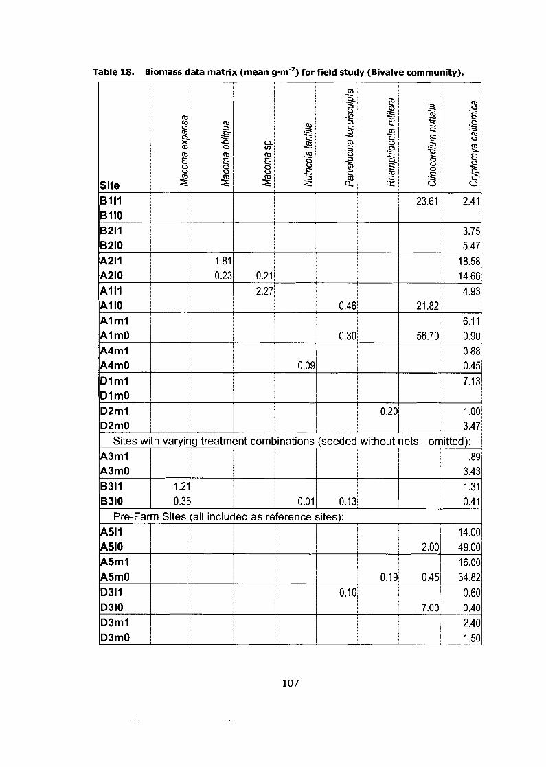
Table 18. Biomass data matrix (mean g.m-2) for field study (Bivalve community).
Sites with varying treatment combinations (seeded without nets - omitted): A3ml I .8E A3m0 3.42 8311 1.21 1.31 B310 0.35 0.01 0.13 1 0.41
Pre-Farm Sites (all included as reference sites): A511 i 14.0C I A510 2.001 49.0C A5ml I I 1 16.0t
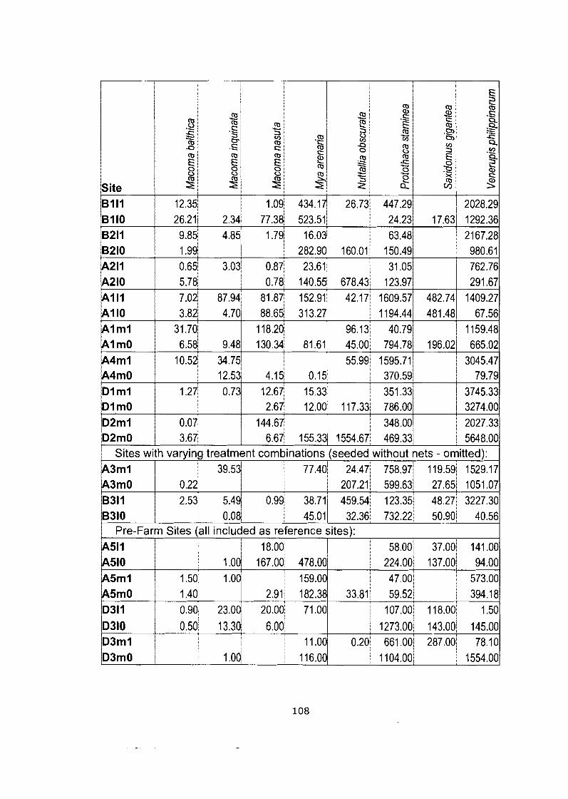
Site B l I1 B l I0 B211 B210 A211 A210 A1 I1 A1 I0
I
Sites with varying treatment combinations (seeded without nets - omitted): A3ml A3m0
Pre-Farm Sites (all included as reference sites):
39.53 0.22
A511 A510 1 1 .OO
18.001 167.00 478.00
77.40
! 58.00 1 224.00
24.47 758.97 207.21 599.63
37.001 141 .OO
137.001 94.00
1 19.59! 1529.17 27.651 1051 -07

Table 19. Data matrix (pooled counts over 5 quadrats) for netting experiment.

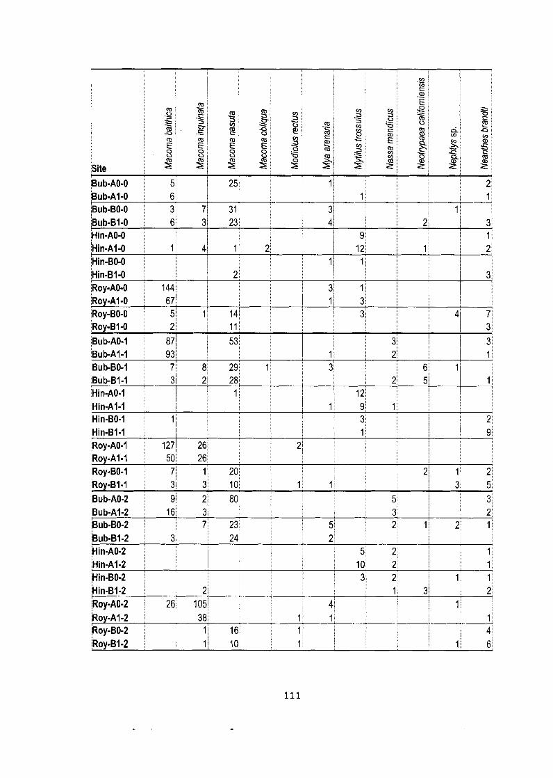
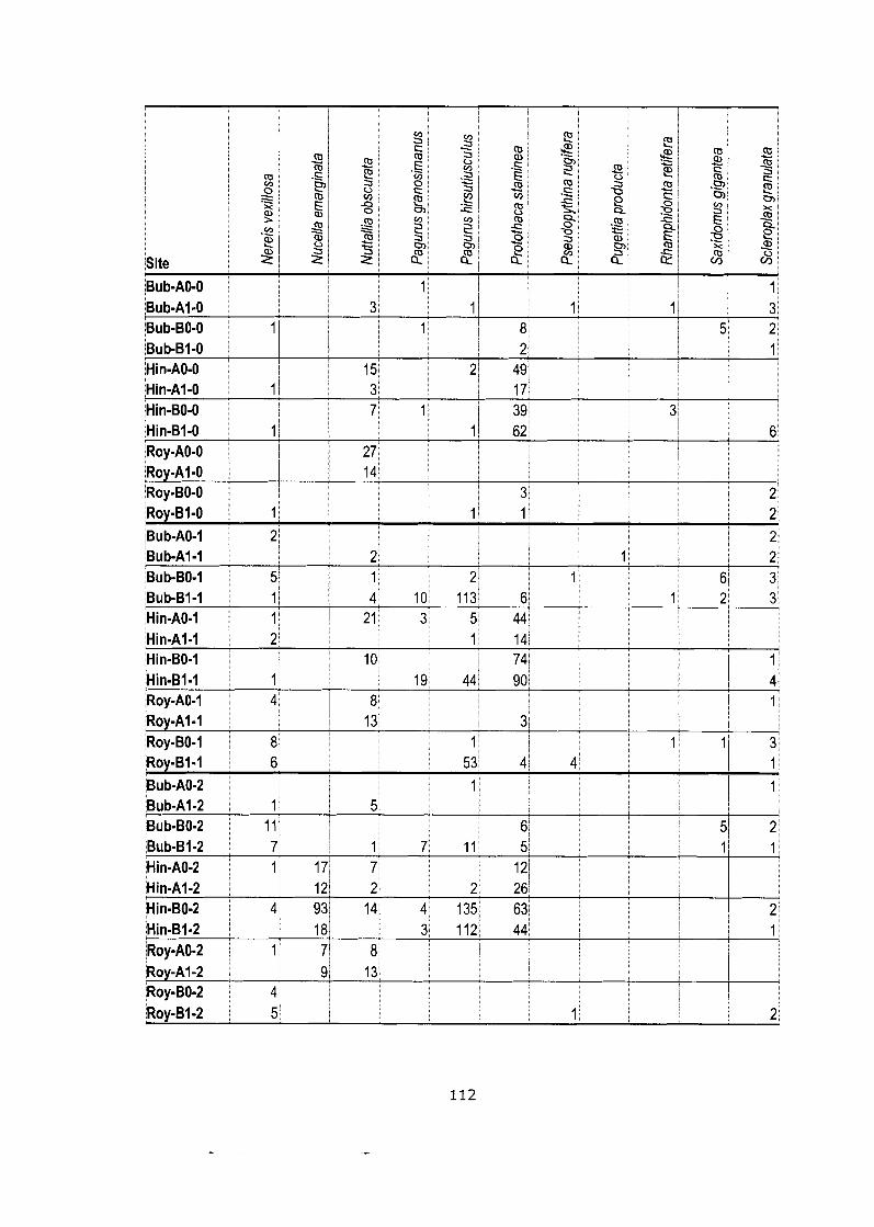
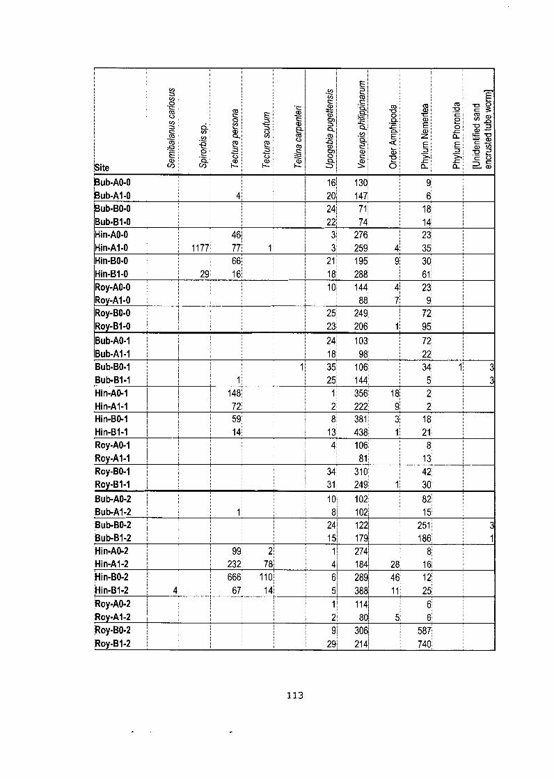
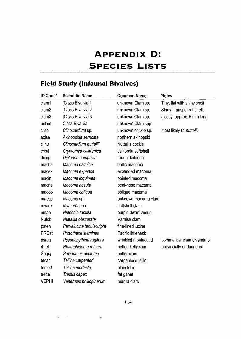
Field Study (Infaunal Bivalves)
ID Code* Scientific Name Common Name Notes
clam1 clam2 clam3 uclam clisp axise clinu crcal diimp macba macex macin macna macob macsp myare nutan Nutob paten PROst
psrug rhret Sagig tecar
temod treca VEPHl
[Class Bivalviall [Class Bivalvial2 [Class Bivalvial3 Class Bivalvia Clinocardium sp. Axinopsida serricata Clinocardium nuttallii Cryptomya californica Diplodonta impolita Macoma balthica Macoma expansa Macoma inquinata Macoma nasuta Macoma obliqua Macoma sp. Mya arenaria Nutricola tantilla Nuttallia obscurata Pamalucina tenuisculpta Protothaca staminea Pseudopythina rugifera Rhamphidonta retifera Saxidomus gigantea Tellina carpenteri
Tellina modesta Tresus capax Venerupis philippinarum
unknown Clam sp. Tiny, flat with shiny shell unknown Clam sp. Shiny, transparent shells unknown Clam sp. glossy, approx. 5 mm long unknown Clam spp. unknown cockle sp. most likely C. nuffallii northern axinopsid Nuttall's cockle california softshell rough diplodon baltic macoma expanded macoma pointed macoma bent-nose macoma oblique macoma unknown macoma clam softshell clam purple dwarf-venus Varnish clam fine-lined lucine Pacific littleneck wrinkled montacutid commensal clam on shrimp netted kellyclam provincially endangered butter clam carpenter's tellin
plain tellin fat gaper
manila clam
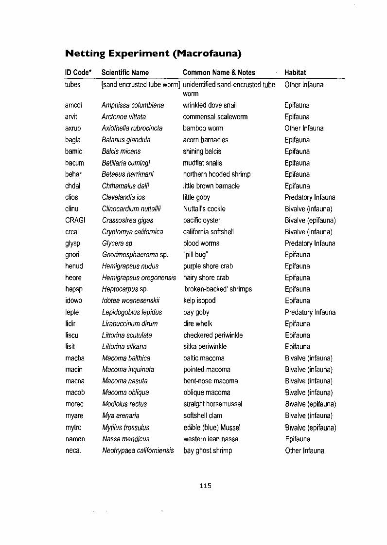
Netting Experiment (Macrofauna)
ID Code* Scientific Name Common Name & Notes Habitat
tubes
amcol
arvit
axrub
bag la
bamic
bacum behar
chdal clios clinu
CRAG1
crcal
~ ~ Y S P
gnori
henud
heore
hepsp idowo
leple lidir
liscu lisit
macba
macin macna
macob morec
myare
mytro namen
necal
[sand encrusted tube worm] unidentified sand-encrusted tube Other lnfauna
Amphissa columbiana
Arctonoe vittata
Axiothella rubrocincta
Balanus glandula
Balcis micans
Batillaria cumingi Betaeus harrimani
Chthamalus dalli
Clevelandia ios
Clinocardium nuttallii
Crassostrea gigas
Cryptomya californica
Glycera sp. Gnorimosphaeroma sp.
Hemigrapsus nudus
Hemigrapsus oregonensis Heptocarpus sp.
ldotea wosnesenskii
Lepidogobius lepidus
Lirabuccinum dirum
Littorina scutulata Littorina sitkana
Macoma balthica
Macoma inquinata
Macoma nasuta
Macoma obliqua Modiolus rectus
Mya arenaria
Mytilus trossulus Nassa mendicus
Neotrypaea californiensis
worm
wrinkled dove snail
commensal scaleworm
bamboo worm
acorn barnacles
shining balcis
mudflat snails northern hooded shrimp
little brown barnacle
little goby
Nuttall's cockle
pacific oyster
california softshell
blood worms "pill bug"
purple shore crab
hairy shore crab
'broken-backed' shrimps
kelp isopod
bay goby dire whelk
checkered periwinkle sitka periwinkle
baltic macoma
pointed macoma bent-nose macoma
oblique macoma straight horsemussel
softshell clam
edible (blue) Mussel western lean nassa
bay ghost shrimp
Epifauna Epifauna
Other lnfauna
Epifauna
Epifauna
Epifauna Epifauna
Epifauna
Predatory lnfauna Bivalve (infauna)
Bivalve (epifauna)
Bivalve (infauna)
Predatory lnfauna Epifauna
Epifauna
Epifauna
Epifauna
Epifauna
Predatory lnfauna Epifauna
Epifauna Epifauna Bivalve (infauna)
Bivalve (infauna) Bivalve (infauna)
Bivalve (infauna) Bivalve (epifauna)
Bivalve (infauna)
Bivalve (epifauna) Epifauna
Other lnfauna
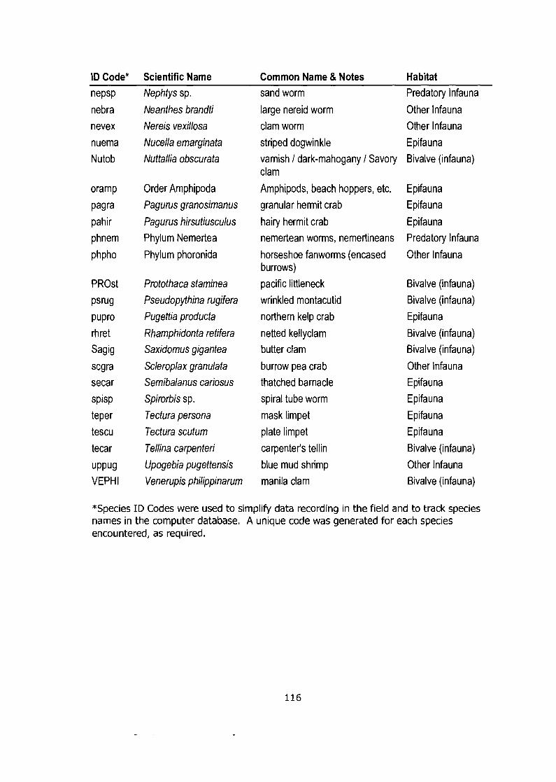
ID Code* Scientific Name Common Name & Notes Habitat
nePsP nebra
nevex nuema
Nutob
oramp
pahir phnem
phpho
PROst
psrug
P u Pro rhret Sagig
scgra secar spisp
teper tescu
tecar
uppug VEPHl
Nephtys sp.
Neanthes brandti
Nereis vexillosa Nucella emarginata
Nuttallia obscurata
Order Amphipoda Pagurus granosimanus
Pagurus hirsutiusculus Phylum Nemertea
Phylum phoronida
Protothaca staminea Pseudopythina rugifera
Pugettia producta
Rhamphidonta retifera Saxidomus gigantea
Scleroplax granulata Semibalanus cariosus Spirorbis sp.
Tectura persona Tectura scutum
Tellina carpenteri
Upogebia pugettensis Venerupis philippinarum
sand worm
large nereid worm
clam worm striped dogwin kle varnish I dark-mahogany I Savory clam
Amphipods, beach hoppers, etc. granular hermit crab
hairy hermit crab nemertean worms, nemertineans
horseshoe fanworms (encased burrows) pacific littleneck
wrinkled montacutid
northern kelp crab
netted kellyclam butter clam
burrow pea crab
thatched barnacle spiral tube worm
mask limpet plate limpet
carpenter's tellin
blue mud shrimp manila clam
Predatory lnfauna
Other lnfauna
Other lnfauna Epifauna Bivalve (infauna)
Epifauna Epifauna
Epifauna Predatory lnfauna
Other lnfauna
Bivalve (infauna) Bivalve (infauna)
Epifauna
Bivalve (infauna) Bivalve (infauna)
Other lnfauna
Epifauna Epifauna
Epifauna Epifauna
Bivalve (infauna)
Other lnfauna Bivalve (infauna)
*Species I D Codes were used to simplify data recording in the field and to track species names in the computer database. A unique code was generated for each species encountered, as required.

Ambrose W. 1991. Are infaunal predators important in structuring marine soft- bottom communities. American Zoologist 31(6):849-860.
Ambrose WG, Jr. 1984. Role of predatory infauna in structuring marine soft-bottom communities. Marine Ecology Progress Series 17(2): 109-115.
BC Parks. 2003. Draft Management Plan for Desolation Sound and Copeland Islands Marine Parks and Tux'wnech Okeover Arm Provincial Park. B.C. Ministry of Water, Land and Air Protection: Environmental Stewardship, Lower Mainland Region. 58 p.
BCSGA. 2003. BC Shellfish Grower's Association - Code of Practice. (February 23 2005; http://www.bcsga.ca/industry~cop.html)
BCSGA. 2004a. BC Shellfish Grower's Association - Industry outlook. (June 17 2004; http://www.bcsga.ca/industry~outlook.html)
BCSGA. 2004b. BC Shellfish Grower's Association - Information Resource Centre. (June 17 2004; http://www.bcsga.ca/industry~irc.html)
Beal BF, Parker MR, Vencile KW. 2001. Seasonal effects of intraspecific density and predator exclusion along a shore-level gradient on survival and growth of juveniles of the soft-shell clam, Mya arenaria L., in Maine, USA. Journal of Experimental Marine Biology and Ecology 264(2):133-169.
Black R, Peterson CH. 1988. Absence of preemption and interference competition for space between large suspension-feeding bivalves and smaller infaunal macroinvertebrates. Journal of Experimental Marine Biology and Ecology 120(3):183-198.
Bourque D, Miron G, Landry T. 2001. Predation on soft-shell clams (Mya arenaria) by the nemertean Cerebratulus lacteus in Atlantic Canada: implications for control measures. Hydrobiologia 456:33-44.
Brose U, Martinez ND, Williams IU. 2003. Estimating species richness: sensitivity to sample coverage and insensitivity to spatial patterns. Ecology 84(9):2364- 2377.
Burnham KP, Overton WS. 1978. Estimation of the size of a closed population when capture probabilities vary among animals. Biometrika 65(3):625-634.
Burnham KP, Overton WS. 1979. Robust estimation of population size when capture probabilities vary among animals. Ecology 60(5):927-936.
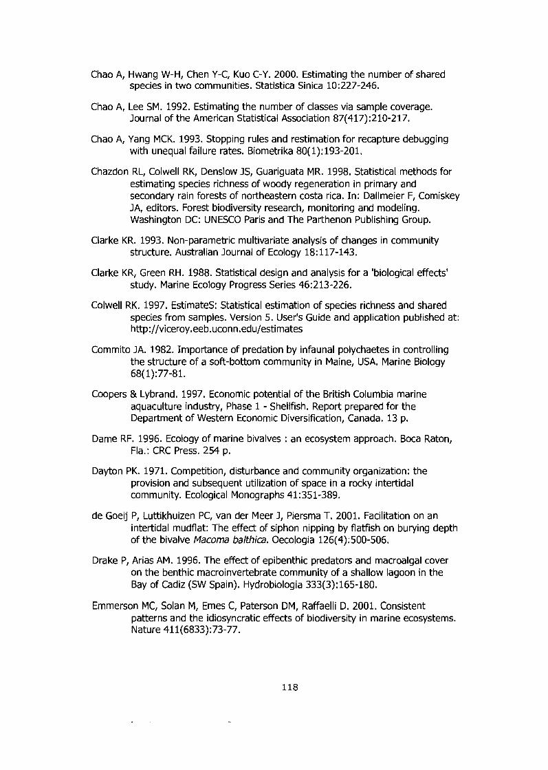
Chao A, Hwang W-HI Chen Y-C, Kuo C-Y. 2000. Estimating the number of shared species in two communities. Statistica Sinica 10:227-246.
Chao A, Lee SM. 1992. Estimating the number of classes via sample coverage. Journal of the American Statistical Association 87(417):210-217.
Chao A, Yang MCK. 1993. Stopping rules and restimation for recapture debugging with unequal failure rates. Biometrika 8O(l): 193-201.
Chazdon RL, Colwell RK, Denslow JS, Guariguata MR. 1998. Statistical methods for estimating species richness of woody regeneration in primary and secondary rain forests of northeastern costa rica. In: Dallmeier F, Comiskey JA, editors. Forest biodiversity research, monitoring and modeling. Washington DC: UNESCO Paris and The Parthenon Publishing Group.
Clarke KR. 1993. Non-parametric multivariate analysis of changes in community structure. Australian Journal of Ecology 18: 117-143.
Clarke KR, Green RH. 1988. Statistical design and analysis for a 'biological effects' study. Marine Ecology Progress Series 46:213-226.
Colwell RK. 1997. Estimates: Statistical estimation of species richness and shared species from samples. Version 5. User's Guide and application published at: http://viceroy.eeb.uconn.edu/estimates
Commito JA. 1982. Importance of predation by infaunal polychaetes in controlling the structure of a soft-bottom community in Maine, USA. Marine Biology 68(1):77-81.
Coopers & Lybrand. 1997. Economic potential of the British Columbia marine aquaculture industry, Phase 1 - Shellfish. Report prepared for the Department of Western Economic Diversification, Canada. 13 p.
Dame RF. 1996. Ecology of marine bivalves : an ecosystem approach. Boca Raton, Fla.: CRC Press. 254 p.
Dayton PK. 1971. Competition, disturbance and community organization: the provision and subsequent utilization of space in a rocky intertidal community. Ecological Monographs 41:351-389.
de Goeij PI Luttikhuizen PC, van der Meer J, Piersma T. 2001. Facilitation on an intertidal mudflat: The effect of siphon nipping by flaffish on burying depth of the bivalve Macoma balthica. Oecologia l26(4): 500-506.
Drake PI Arias AM. 1996. The effect of epibenthic predators and macroalgal cover on the benthic macroinvertebrate community of a shallow lagoon in the Bay of Cadiz (SW Spain). Hydrobiologia 333(3):165-180.
Emmerson MC, Solan MI Emes C, Paterson DM, Raffaelli D. 2001. Consistent patterns and the idiosyncratic effects of biodiversity in marine ecosystems. Nature 411(6833):73-77.
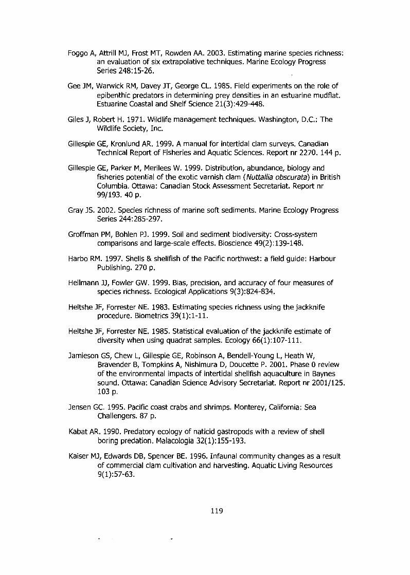
Foggo A, Attrill MJ, Frost MT, Rowden AA. 2003. Estimating marine species richness: an evaluation of six extrapolative techniques. Marine Ecology Progress Series 248: 15-26,
Gee JM, Warwick RM, Davey JT, George CL. 1985. Field experiments on the role of epibenthic predators in determining prey densities in an estuarine mudflat. Estuarine Coastal and Shelf Science 21(3):429-448.
Giles J, Robert H. 1971. Wildlife management techniques. Washington, D.C.: The Wildlife Society, Inc.
Gillespie GE, Kronlund AR. 1999. A manual for intertidal clam surveys. Canadian Technical Report of Fisheries and Aquatic Sciences. Report n r 2270. 144 p.
Gillespie GE, Parker MI Merilees W. 1999. Distribution, abundance, biology and fisheries potential of the exotic varnish clam (Nultallia obscurata) in British Columbia. Ottawa: Canadian Stock Assessment Secretariat. Report nr 991193. 40 p.
Gray JS. 2002. Species richness of marine soft sediments. Marine Ecology Progress Series 244:285-297.
Groffman PM, Bohlen PJ. 1999. Soil and sediment biodiversity: Cross-system comparisons and large-scale effects. Bioscience 49(2): 139-148.
Harbo RM. 1997. Shells & shellfish of the Pacific northwest: a field guide: Harbour Publishing. 270 p.
Hellmann JJ, Fowler GW. 1999. Bias, precision, and accuracy of four measures of species richness. Ecological Applications 9(3):824-834.
Heltshe JF, Forrester NE. 1983. Estimating species richness using the jackknife procedure. Biometrics 39(1): 1-11.
Heltshe JF, Forrester NE. 1985. Statistical evaluation of the jackknife estimate of diversity when using quadrat samples. Ecology 66(1): 107-111.
Jamieson GS, Chew L, Gillespie GE, Robinson A, Bendell-Young L, Heath W, Bravender B, Tompkins A, Nishimura Dl Doucette P. 2001. Phase 0 review of the environmental impacts of intertidal shellfish aquaculture in Baynes sound. Ottawa: Canadian Science Advisory Secretariat. Report nr 20011125. 103 p.
Jensen GC. 1995. Pacific coast crabs and shrimps. Monterey, California: Sea Challengers. 87 p.
Kabat AR. 1990. Predatory ecology of naticid gastropods with a review of shell boring predation. Malacologia 32(1): 155-193.
Kaiser MJ, Edwards DB, Spencer BE. 1996. Infaunal community changes as a result of commercial clam cultivation and harvesting. Aquatic Living Resources 9(1):57-63.
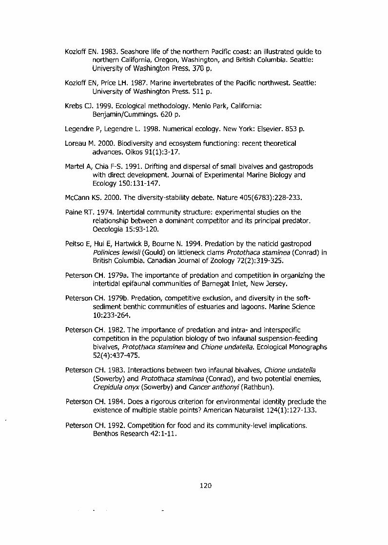
Kozloff EN. 1983. Seashore life of the northern Pacific coast: an illustrated guide to northern California, Oregon, Washington, and British Columbia. Seattle: University of Washington Press. 370 p.
Kozloff EN, Price LH. 1987. Marine invertebrates of the Pacific northwest. Seattle: University of Washington Press. 511 p.
Krebs CJ. 1999. Ecological methodology. Menlo Park, California: Benjamin/Cummings. 620 p.
Legendre P, Legendre L. 1998. Numerical ecology. New York: Elsevier. 853 p.
Loreau M. 2000. Biodiversity and ecosystem functioning: recent theoretical advances. Oikos 91(1):3-17.
Martel A, Chia F-S. 1991. Drifting and dispersal of small bivalves and gastropods with direct development. Journal of Experimental Marine Biology and Ecology 150: 131-147.
McCann KS. 2000. The diversity-stability debate. Nature 405(6783):228-233.
Paine RT. 1974. Intertidal community structure: experimental studies on the relationship between a dominant competitor and its principal predator. Oecologia 15:93-120.
Peitso El Hui El Harhvick B, Bourne N. 1994. Predation by the naticid gastropod Polinices lewisii (Gould) on littleneck clams Protothaca staminea (Conrad) in British Columbia. Canadian Journal of Zoology 72(2):319-325.
Peterson CH. 1979a. The importance of predation and competition in organizing the intertidal epifaunal communities of Barnegat Inlet, New Jersey.
Peterson CH. 1979b. Predation, competitive exclusion, and diversity in the soft- sediment benthic communities of estuaries and lagoons. Marine Science 10:233-264.
Peterson CH. 1982. The importance of predation and intra- and interspecific competition in the population biology of two infaunal suspension-feeding bivalves, Protothaca staminea and Chione undatella. Ecological Monographs 52(4):437-475.
Peterson CH. 1983. Interactions between two infaunal bivalves, Chione undatella (Sowerby) and Protothaca staminea (Conrad), and two potential enemies, Crepidula onyx (Sowerby) and Cancer anthonyi (Rathbu n).
Peterson CH. 1984. Does a rigorous criterion for environmental identity preclude the existence of multiple stable points? American Naturalist 124(1): 127-133.
Peterson CH. 1992. Competition for food and its community-level implications. Benthos Research 42: 1-11.
Peterson CHI Andre SV. 1980. An experimental analysis of interspecific competition among marine filter feeders in a soft-sediment environment. Ecology 6 l ( l ) : 129-139.
Peterson CHI Beal BF. 1989. Bivalve growth and higher order interactions: importance of density, site and time. Ecology 70(5):1390-1404.
Peterson CHI Black R. 1991. Preliminary evidence for progressive sestonic food depleton in incoming tide over a broad tidal sand flat. Estuarine Coastal and Shelf Science 32(4):405.
Posey MH. 1986. Predation on a burrowing shrimp: distribution and community consequences. Journal of Experimental Marine Biology and Ecology 103(1- 3): 143-161.
Posey MH, Alphin TD, Cahoon LB, Lindquist DG, Mallin MA, Nevers MB. 2002. Top- down versus bottom-up limitation in benthic infaunal communities: direct and indirect effects. Estuaries 25(5):999-1014.
Purvis A, Hector A. 2000. Getting the measure of biodiversity. Nature 405(6783):212-219.
Quammen ML. 1984. Predation by shorebirds, fish, and crabs on invertebrates in intertidal mudflats: an experimental test. Ecology 65(2):529-537.
Quayle DB, Bourne N. 1972. The clam fisheries of British Columbia. Ottawa: Environment Canada, Fisheries Research Board of Canada. 70 p.
Reise K. 1985. Predator control in marine tidal sediments. European Marine Biology Symposium 19:3ll-321.
Richards MG, Huxham MI Bryant A. 1999. Predation: a causal mechanism for variability in intertidal bivalve populations. Journal of Experimental Marine Biology and Ecology 24l(2): 159-177.
Seitz RD, Lipcius RN, Hines AH, Eggleston DB. 2001. Density-dependent predation, habitat variation, and the persistence of marine bivalve prey. Ecology 82(9):2435-2451.
Sept JD. 1999. The beachcomber's guide to seashore life in the Pacific northwest. Madeira Park: Harbour Publishing. 235 p.
Sewell MA. 1996. Detection of the impact of predation by migratory shorebirds: an experimental test in the Fraser River estuary, British Columbia (Canada). Marine Ecology Progress Series 144(1-3):23-40.
Snelgrove PVR. 1999. Getting to the bottom of marine biodiversity: sedimentary habitats. Bioscience 49(2): 129-138.
Sokal RR, Rohlf FJ. 1981. Biometry the principles and practice of statistics in biological research 3rd Edition. New York: W. H. Freeman and Company. 887 p.
Spencer BE, Edwards DB, Millican PF. 1992. Protecting manila clam (Tapes philippinarum) beds with plastic netting. Aquaculture 105(3-4):251-268.
Spencer BE, Kaiser MJ, Edwards DB. 1996. The effect of manila clam cultivation on an intertidal benthic community: the early cultivation phase. Aquaculture Research 27(4):261-276.
Spencer BE, Kaiser MJ, Edwards DB. 1997. Ecological effects of intertidal manila clam cultivation: observations at the end of the cultivation phase. Journal of Applied Ecology 34(2):444-452.
Spencer BE, Kaiser MJ, Edwards DB. 1998. Intertidal clam harvesting: benthic community change and recovery. Aquaculture Research 29(6):429-437.
Summerson HC, Peterson CH. 1984. Role of predation in organizing benthic communities of a temperate-zone seagrass bed. Marine Ecology Progress Series 15(1-2):63-77.
Tilman D, Reich PB, Knops J, Wedin D, Mielke T, Lehman C. 2001. Diversity and productivity in a long-term grassland experiment. Science 294(5543):843-845.
Vargas JA. 1988. Community structure of macrobenthos and the results of macropredator exclusion on a tropical intertidal mud flat. Revista de Biologia Tropical 36(2A):287-308.
Wentworth CK. 1922. A scale of grade and class terms for clastic sediments. Journal of Geology 30:377-392.
Wiltse WI. 1980. Effects of Polinices duplicatus (Gastropoda: Naticidae) on infaunal community structure at Barnstable Harbor, Massachusetts, USA. Marine Biology 56(4):301-310.
Worm B, Duffy JE. 2003. Biodiversity, productivity and stability in real food webs. Trends in Ecology and Evolution 18(12):628-632.
Yachi S, Loreau M. 1999. Biodiversity and ecosystem productivity in a fluctuating environment: the insurance hypothesis. Proceedings of the National Academy of Sciences of the United States of America 96(4):1463-1468.