Macroeconomic Factors and Sectoral Indices: A …pakacademicsearch.com/pdf-files/ech/517/132-152 Vol 4, No 17 (2012...Macroeconomic Factors and Sectoral Indices: ... These sectors

European Journal of Business and Management www.iiste.org ISSN 2222-1905 (Paper) ISSN 2222-2839 (Online) Vol 4, No.17, 2012

132

Macroeconomic Factors and Sectoral Indices: A Study of Karachi

Stock Exchange (Pakistan)

SADIA SAEED

Faculty of Management Sciences, National University of Modern Languages, Islamabad, Pakistan

E-mail of corresponding author: [email protected]

ABSTRACT

The primary purpose of this study is to examine the impact of macroeconomic variables on stock returns by applying

multifactor model within an APT frame work. This study consists of five macroeconomic variables Money Supply,

Exchange Rate, Industrial Production, Short Term Interest Rate and Oil prices. Nine sectors are selected for the study

on the basis of data availability on the Karachi Stock Exchange 100 index. These sectors are Oil and Gas, Textile

Composite, Jute, Cement, Cable and electrical Goods, Automobile, Chemical and Pharmaceutical, Leasing and Glass

and Ceramics. The closing prices of each firm of each sector are obtained for the period of ten years starting from

June 2000- June 2010. Descriptive statistics are performed for the temporal properties of data and Augmented

Dickey Fuller (ADF) is employed to check the stationarity of data. Multicollinearity has been tested among

independent variables through correlation matrix. Diagnostic results show that data has no econometric problem

therefore Ordinary Least Square has been used to analyze the impact of macroeconomic variables on the returns. The

result reveals that macro-economic variables have significant impact on the returns of sectors but their contribution

to bring variation in their returns is very small. Only Short Term Interest Rate has a significant impact on returns of

various sectors where as Exchange Rate and Oil prices have significant impact on specific sectors like and Oil and

Gas sector, Automobile and Cable and Electronics. This sectoral study also documents the usefulness of the

multifactor model as compared to a single index model.

Key Words: Arbitrage Pricing Theory (APT), Ordinary Least Square (OLS), Augmented Dickey Fuller Test (ADF),

Macroeconomic Variables, Sectoral Indices.

1.0 INTRODUCTION

In developed Capital markets there is close association between Macroeconomic forces and stock prices and the

literature available on that study since 1970s. The variation in stock prices has been studied by multi beta model

named as Arbitrage Pricing Theory (APT).These studies have a focus on developed markets. After 1980s the

association between stock prices and macroeconomic forces has been examined in emerging markets. Menike (2006)

(as cited by Ali 2011).Emerging stock markets has two characteristics first these are shallow and second these are

unstable. These two features of emerging stock markets enforce the macroeconomic forces to play an important role

in bullish and bearish trend of stock market. Moreover oversensitivity in stock returns to macroeconomic forces is

created by low volume of trade and limited available public information along with shallowness and unstable nature

of emerging stock markets.

The emerging markets have been attentively taken by investors over the past decade. It is noticed that the returns in

emerging stock markets is greater as compared to the developed markets. Pakistan has also emerging stock market

due to shallowness and instability in its stock markets. A crowd of problems stood in the way of Pakistan which

destroyed its economic potential since 1947. Many problems aroused in the economic progress of country like Fights

among religious sects, outmoded bureaucratic procedure, Custom duties, Counterproductive tax rates and strategic

approach of Government kept away Pakistani stock markets from foreign investment.

Every investor wants to get better return on its investment. There are many investment opportunities for investment

in a country. Investment in stock market is one of them. The return, when any investor invests in stock market

depends on various factors. The precise number of these factors is not known yet. Literature on Capital markets

reveals that a large no of factors are involved in the determinant of equity prices. The suggestion available in the

literature is, different variables are involved in bringing variation in the stock returns.

Many studies of different researchers are available in the literature about the relationship between macroeconomic

variables and stock prices .These studies have a focus on composite index rather than sector index .This study is


133

different from the other studies in a way that it investigates the impact of macroeconomic forces on sectoral indices.

In literature there exist some traces of investigation between macroeconomic factors and returns on specific sectors.

Ball and Brown (1980) showed in their study that the behavior of stock prices in mining sector in Australian Stock

Market is abnormal. They concluded that the return on mining sector as compared to the other sector is high without

earning risk premium.

Faff and Chan (1988) (as cited by Muneer, Zaheer and Rehman 2011) revealed that there is a strong impact of

macroeconomic variables on the returns of gold industry. Their multi factor model is comprised of three

macroeconomic factors gold rate, exchange rate and interest rate. They concluded that these macroeconomic factors

have a strong impact on returns of gold.

In the study five macroeconomic variables are taken Money Supply, Short term interest rate, Industrial production,

and Exchange rate and oil prices. These macroeconomic variables have been selected on the basis of literature. The

sectors which have been selected in doing research are Jute, Fertilizer, Pharmaceutical, Automobile, Electrical goods

an Oil and gas sector, Leasing, Textile Composite and Glass and Ceramics. The study attempts to determine the

impact of macroeconomic variables on various sectors listed on Karachi Stock Exchange.

This study is a contribution to the literature by analyzing the impact of macroeconomic factors on various sectors.

The results of this study is helpful in determining the behavior of returns of various factors in response to change in

macroeconomic forces such as Short Term Interest Rate , Oil Prices, Exchange Rate, Money Supply and Industrial

production. Moreover the outcomes of the study are also helpful in designing the economic and financial policy by

taking in to account the performance of various sectors in stock market.

This paper is organized in five sections. First section shows the introduction and importance of research. Second

section indicates the literature review about the relationship between macroeconomic forces and returns of Stocks.

Research Methodology along with hypothesis is presented in section three. Empirical Results and Discussion are

narrated in section Four. Section five reveals the Conclusion, Recommendations and future implications of the study.

1.2 Objectives of study

The specific objectives of study are

• To examine the impact of macroeconomic variables on the returns of different sectors listed on Karachi

Stock Exchange.

• To know the intensity of macroeconomic variable on the returns of different sectors listed on Karachi Stock

Exchange.

2.0 LITERATURE REVIEW

In literature two models have been usually employed in determining the risk return relationship Capital Asset Pricing

Model (CAPM) and Arbitrage Pricing Theory (APT).CAPM was developed by Sharpe (1963). It measures the risk

return relationship on the basis of single factor. Therefore it is considered as inappropriate model in predicting the

risk return relationship. On the other hand APT considers various micro and macro-economic factors in measuring

the risk return relationship. APT is based upon the fewer assumptions as compared to CAPM. A lot of studies in

literature used APT and CAPM model in demonstrating the relationship between risk factors and returns of the stock.

A brief overview of these studies is illustrated below.

Chen et al. (1986) explained the returns of stocks by taking in to account the macroeconomic forces in APT

framework. The macroeconomic variables included in his study were spread between long and short interest rates,

expected and unexpected inflation, industrial production and the spread between returns on high and low grade bonds.

His findings were that these macroeconomic factors had played a significant role in explaining the variability in

stock returns.

Chen (1991) modified the APT model by using macroeconomic factors in determining the risk return relationship.

The macroeconomic factors used in his study were lagged, the default risk premium, short term interest rates and

market dividend price ratio, production growth rate and the term premium for the period 1954 to 1986. His result

showed that the returns of the stocks had been dependent upon these macroeconomic factors and these factors were

negatively correlated to excess market return.


134

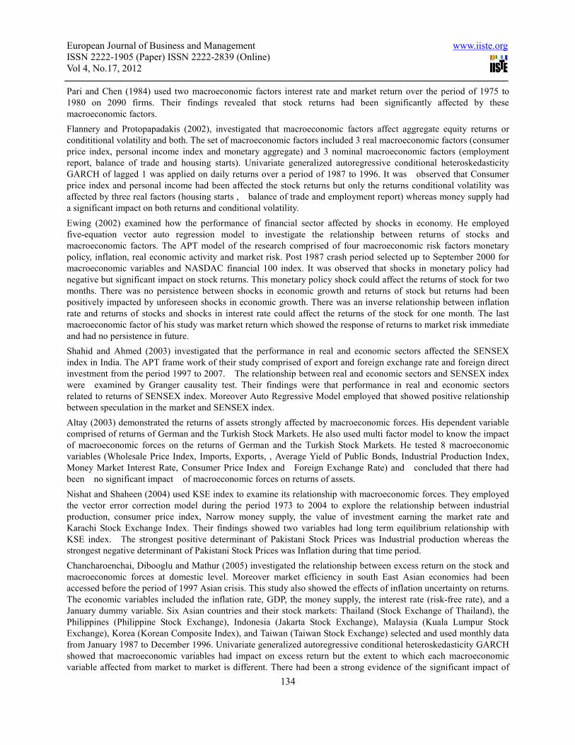
Pari and Chen (1984) used two macroeconomic factors interest rate and market return over the period of 1975 to

1980 on 2090 firms. Their findings revealed that stock returns had been significantly affected by these

macroeconomic factors.

Flannery and Protopapadakis (2002), investigated that macroeconomic factors affect aggregate equity returns or

condititional volatility and both. The set of macroeconomic factors included 3 real macroeconomic factors (consumer

price index, personal income index and monetary aggregate) and 3 nominal macroeconomic factors (employment

report, balance of trade and housing starts). Univariate generalized autoregressive conditional heteroskedasticity

GARCH of lagged 1 was applied on daily returns over a period of 1987 to 1996. It was observed that Consumer

price index and personal income had been affected the stock returns but only the returns conditional volatility was

affected by three real factors (housing starts , balance of trade and employment report) whereas money supply had

a significant impact on both returns and conditional volatility.

Ewing (2002) examined how the performance of financial sector affected by shocks in economy. He employed

five-equation vector auto regression model to investigate the relationship between returns of stocks and

macroeconomic factors. The APT model of the research comprised of four macroeconomic risk factors monetary

policy, inflation, real economic activity and market risk. Post 1987 crash period selected up to September 2000 for

macroeconomic variables and NASDAC financial 100 index. It was observed that shocks in monetary policy had

negative but significant impact on stock returns. This monetary policy shock could affect the returns of stock for two

months. There was no persistence between shocks in economic growth and returns of stock but returns had been

positively impacted by unforeseen shocks in economic growth. There was an inverse relationship between inflation

rate and returns of stocks and shocks in interest rate could affect the returns of the stock for one month. The last

macroeconomic factor of his study was market return which showed the response of returns to market risk immediate

and had no persistence in future.

Shahid and Ahmed (2003) investigated that the performance in real and economic sectors affected the SENSEX

index in India. The APT frame work of their study comprised of export and foreign exchange rate and foreign direct

investment from the period 1997 to 2007. The relationship between real and economic sectors and SENSEX index

were examined by Granger causality test. Their findings were that performance in real and economic sectors

related to returns of SENSEX index. Moreover Auto Regressive Model employed that showed positive relationship

between speculation in the market and SENSEX index.

Altay (2003) demonstrated the returns of assets strongly affected by macroeconomic forces. His dependent variable

comprised of returns of German and the Turkish Stock Markets. He also used multi factor model to know the impact

of macroeconomic forces on the returns of German and the Turkish Stock Markets. He tested 8 macroeconomic

variables (Wholesale Price Index, Imports, Exports, , Average Yield of Public Bonds, Industrial Production Index,

Money Market Interest Rate, Consumer Price Index and Foreign Exchange Rate) and concluded that there had

been no significant impact of macroeconomic forces on returns of assets.

Nishat and Shaheen (2004) used KSE index to examine its relationship with macroeconomic forces. They employed

the vector error correction model during the period 1973 to 2004 to explore the relationship between industrial

production, consumer price index, Narrow money supply, the value of investment earning the market rate and

Karachi Stock Exchange Index. Their findings showed two variables had long term equilibrium relationship with

KSE index. The strongest positive determinant of Pakistani Stock Prices was Industrial production whereas the

strongest negative determinant of Pakistani Stock Prices was Inflation during that time period.

Chancharoenchai, Dibooglu and Mathur (2005) investigated the relationship between excess return on the stock and

macroeconomic forces at domestic level. Moreover market efficiency in south East Asian economies had been

accessed before the period of 1997 Asian crisis. This study also showed the effects of inflation uncertainty on returns.

The economic variables included the inflation rate, GDP, the money supply, the interest rate (risk-free rate), and a

January dummy variable. Six Asian countries and their stock markets: Thailand (Stock Exchange of Thailand), the

Philippines (Philippine Stock Exchange), Indonesia (Jakarta Stock Exchange), Malaysia (Kuala Lumpur Stock

Exchange), Korea (Korean Composite Index), and Taiwan (Taiwan Stock Exchange) selected and used monthly data

from January 1987 to December 1996. Univariate generalized autoregressive conditional heteroskedasticity GARCH

showed that macroeconomic variables had impact on excess return but the extent to which each macroeconomic

variable affected from market to market is different. There had been a strong evidence of the significant impact of


135

inflation uncertainty on monthly stock excess returns or on their time-varying variance.

Rehman and Saeedullah (2005) demonstrated the impact of macroeconomic forces on the returns of Cement industry.

In this paper seven cement firms were selected on the basis of data availability, Profitability and performance on

Karachi Stock Exchange 100 index. The results of Multi- Index model showed that only Karachi Stock Exchange

100 index had a significant impact on stock returns of cement while other industry variables did not show any

contribution in bringing variation in stock returns of cement firms.

Guns and Cukor (2007), employed the APT model on the returns of London Stock Exchange to investigate the

impact of macroeconomic factors on them.They used seven macro economic variables (uncertainty in inflation,

Uncertainty in sectoral industrial production, risk premium,interest rate, exchange rate, money supply,

unforeseensectoral dividend yield, a residual error for industry portfolio) in their study. They tested the validity of

APT model and their findings showed that the returns of London Stock Exchange had been dependent upon these

macroeconomic factors.

TursoyGunsol and Rjoub (2008)used monthly data form February 2001 to September 2005 to test the validity of APT

model in Istanbul Stock Exchange (ISE).Eleven industrial portfolios examined in response to change in

macroeconomic forces. The APT model comprised of thirteen macroeconomic variables crude oil price, consumer

price index, import, export, gold price, exchange rate, , gross domestic product, foreign reserve, unemployment rate

market pressure index, Industrial production, interest rateand money supply. They concluded that the returns of

Istanbul Stock Exchange (ISE) had not been affected by these macroeconomic factors.

Other studies included, Hussain, Mehmood and Ali (2009) measured the relationship between equity prices and

macroeconomic forces. Similarly, the impact of macroeconomic forces on the returns of banking sector has been

analyzed by Butt, Rehman and Ahmed (2007). Moreover Ihsan et al (2007) used financial and macroeconomic

variables in determining the risk return relationship. Ahmed and Farooq (2008) used terrorisam factor such as 9/11

for determining the stock volatility of Karachi Stock Exchange. Trading volume used by Khan and Rizwan (2008)

for measring the stock market behavior

2.1 Theoretical Framework

The Theoretical Framework of the study is based upon APT. It is a general theory of pricing of asset. According to

this theory the return of the asset is a linear combination of non-diversifiable macroeconomic factors. These

macroeconomic factors are the risk factors. The changes in the risk factors are the source of earning risk premium

which affect the returns of the stock. The multifactor model of the study is developed under the guidance of literature.

Macro economic factors that can potentially affect the returns of the asset have been identified from the literature.

These macroeconomic factors are short term interest rate, Money supply M2, Exchange rate, Oil prices and Industrial

Production as some principal determinant of variability in stock returns. This study investigates the impact of

macroeconomic factors on sectoral returns. The sectors which have been selected in the study are Jute, Cement,

Pharmaceutical, Automobile, Electrical goods and Oil and gas sector where as sub sectors which have been elected

Independent Variable

Macroeconomic Variable

• Money Supply

• Exchange Rate

• Industrial Production

• Short Term Interest

Rate

• Oil Prices

Dependent Variable

Sectorial Indices

• Oil & Gas Sector

• Textile Composite

• Jute

• Cement

• Automobile

• Cable & Electrical Goods

• Chemical & pharmaceutical

• Leasing

• Glass & Ceramics


136

for the study are Leasing, Textile Composite and Glass and Ceramics. This is a sectoral study in emerging stock

market of Pakistan which has a different structure as compared to developed stock markets. Therefore it is critical to

find out the impact of macroeconomic factors and sactoral returns because emerging markets return respond

differently in response to macroeconomic variables as compared to developed markets. The diagrammatic

relationship between independent and dependent variables is given below

2.2 Hypotheses

On the basis of research theory following Hypothesis has been developed.

H1: Macroeconomic variables have significant impact on Oil and Gas Sector

H2: Macroeconomic variables have significant impact on Textile Composite

H3: Macroeconomic variables have significant impact on Jute

H4: Macroeconomic variables have significant impact on Cement

H5: Macroeconomic variables have significant impact on Automobile

H6: Macroeconomic variables have significant impact on Cable and Electronics

H7: Macroeconomic variables have significant impact on Chemical and Pharmaceutical

H8: Macroeconomic variables have significant impact on Leasing

H9: Macroeconomic variables have significant impact on Glass and Ceramics

3.0 RESEARCH METHODOLOGY

3.1 DATA DESCRIPTION

This study explores the impact of macroeconomic variables on the returns of nine sectors for the period of June 2000

to June 2010 by using monthly data. The macro economic variables included in the study are Money supply M2,

Exchange rate, Industrial production, Short term interest rate and Oil prices. Monthly time series of elected sectors

for the same period has been taken for explaining the impact of macroeconomic factors on their returns.

Secondary data has been used in the study. The selection criteria of sectors are dependent upon the availability of

data in business recorder. The indexes of these sectors have been calculated by equally weighted method. The data

for each firm in a sector has been obtained from the web sites of business recorder and Karachi stock exchange for

the period of ten years starting from June 2000- June 2010. State bank of Pakistan, Federal bureau of statistics and

various editions of economic survey of Pakistan have been consulted for calculating the data of macroeconomic risk

factors such as short term interest rate, Exchange rate, Oil prices, Money Supply M2, and industrial production. This

study includes macroeconomic variables as independent variables and stock returns of various sectors as dependent

variables.

3.1.1. Independent Variables

Exchange Rate

Exchange rate means the rate at which one currency is converted to another. The exchange rate is as end of month Rs.

/US$. The relationship between exchange rate and return is negative. If exchange rate of home currency with

respect to dollar increases it will affect the cash flows in a negative manner and reduce the return. If the sector

involve in export then the relationship of exchange rate with the returns will be positive.

Money Supply M2

Money Supply includes currency in circulation, plus saving and small time deposit, Overnight repos at commercial

banks and non-institution money market. This is the key economic indicator since it is not as narrow as M1 and still

relatively easy to track. The relationship of Money supply with the returns is positive in the short run as the liquidity

is increased due to increase in the money supply. In the long run increase in money supply leads to increase the

inflation which affects the return in a negative manner.

Industrial Production

The economic growth in real sector or overall economic activity is indicated by Industrial production index. As the


137

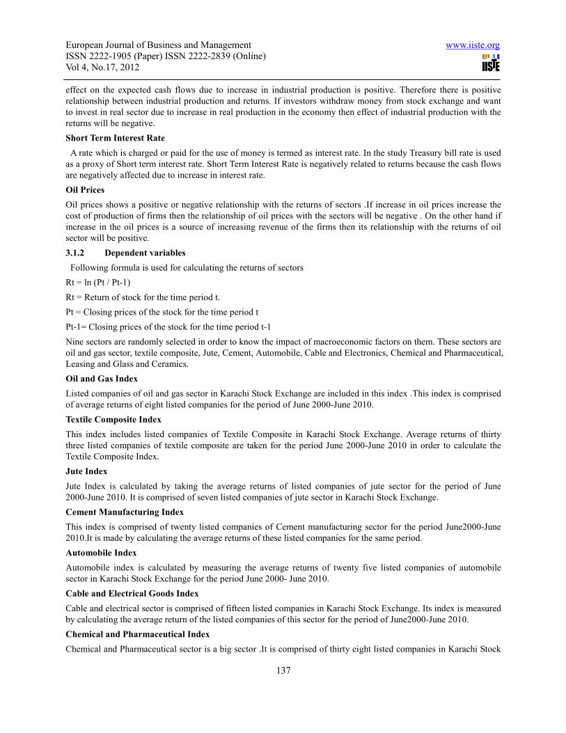
effect on the expected cash flows due to increase in industrial production is positive. Therefore there is positive

relationship between industrial production and returns. If investors withdraw money from stock exchange and want

to invest in real sector due to increase in real production in the economy then effect of industrial production with the

returns will be negative.

Short Term Interest Rate

A rate which is charged or paid for the use of money is termed as interest rate. In the study Treasury bill rate is used

as a proxy of Short term interest rate. Short Term Interest Rate is negatively related to returns because the cash flows

are negatively affected due to increase in interest rate.

Oil Prices

Oil prices shows a positive or negative relationship with the returns of sectors .If increase in oil prices increase the

cost of production of firms then the relationship of oil prices with the sectors will be negative . On the other hand if

increase in the oil prices is a source of increasing revenue of the firms then its relationship with the returns of oil

sector will be positive.

3.1.2 Dependent variables

Following formula is used for calculating the returns of sectors

Rt = ln (Pt / Pt-1)

Rt = Return of stock for the time period t.

Pt = Closing prices of the stock for the time period t

Pt-1= Closing prices of the stock for the time period t-1

Nine sectors are randomly selected in order to know the impact of macroeconomic factors on them. These sectors are

oil and gas sector, textile composite, Jute, Cement, Automobile, Cable and Electronics, Chemical and Pharmaceutical,

Leasing and Glass and Ceramics.

Oil and Gas Index

Listed companies of oil and gas sector in Karachi Stock Exchange are included in this index .This index is comprised

of average returns of eight listed companies for the period of June 2000-June 2010.

Textile Composite Index

This index includes listed companies of Textile Composite in Karachi Stock Exchange. Average returns of thirty

three listed companies of textile composite are taken for the period June 2000-June 2010 in order to calculate the

Textile Composite Index.

Jute Index

Jute Index is calculated by taking the average returns of listed companies of jute sector for the period of June

2000-June 2010. It is comprised of seven listed companies of jute sector in Karachi Stock Exchange.

Cement Manufacturing Index

This index is comprised of twenty listed companies of Cement manufacturing sector for the period June2000-June

2010.It is made by calculating the average returns of these listed companies for the same period.

Automobile Index

Automobile index is calculated by measuring the average returns of twenty five listed companies of automobile

sector in Karachi Stock Exchange for the period June 2000- June 2010.

Cable and Electrical Goods Index

Cable and electrical sector is comprised of fifteen listed companies in Karachi Stock Exchange. Its index is measured

by calculating the average return of the listed companies of this sector for the period of June2000-June 2010.

Chemical and Pharmaceutical Index

Chemical and Pharmaceutical sector is a big sector .It is comprised of thirty eight listed companies in Karachi Stock


138

Exchange. Its index is calculated by measuring the average returns of the listed companies of this sector for the

period June2000-June2010.

Leasing Index

Leasing sector is also a big sector. It includes thirty two listed companies in Karachi Stock Exchange. Leasing index

is measured by taking the average returns of these thirty two listed companies for the period June2000-June2010.

Glass and Ceramics Index

Glass and Ceramics Sector include ten listed companies in Karachi Stock Exchange. Its index is made by calculating

the average returns of the listed companies of this sector for the period June2000-June 2010

3.2 Methodology

Four steps have been performed in methodology framework of the study. The chronological properties such as Mean,

standard deviation, skewness and Kurtosis of each variable are analyzed through descriptive statistics. The second

step is to create correlation matrix in order to show the relationship among independent variables. The third step is to

analyze the stationarity of data by the Augmented Dickey Fuller (ADF). This test is helpful in establishing the order

of integration of the variables under study. A variable is said to be integrated of order d, I(d), if it is stationary after

differencing d times. It means that the variable that is integrated of order greater or equal to 1 is non-stationary. The

ADF Test is based on the following equation:

k

∆xt = α + βt + ρ Xt -1 + k фi ∆Xt -1 + 1t (1)

i=1

Where x is the natural logarithm of the series under consideration and t is a trend term, ρ and ф are the parameters to

be estimated and 1 is the error term. In ADF unit root test the null hypothesis is that the series is non-stationary which

is either accepted or rejected by comparing the t-statistics of the lagged term Xt -1 with the critical values given in

Mackinnon (1991). If the t-value is less than the critical value then the null hypothesis of a unit root (i.e. the series is

nonstationary) is accepted. If this is the case the first difference of the series is examined and if the t-value is greater

than the critical value then the null hypothesis is rejected and the series is considered stationary with the assumption

that the series is integrated of order one I (1). Once the order of integration is established for each variable, the next

step is to investigate the effect of economic variables on the stock market returns of individual firms and industry as

a whole.

The last step is to know the effect of macroeconomic factors on sectors ordinary least square is employed. OLS

stands for Ordinary Least Squares, the standard linear regression procedure. One estimates a parameter from data and

applying the linear model

y = a+ bx + e

y = Dependent variable that is return of sector.

a = Constant

x = independent variable that is macroeconomic factors.

b = sensitivity of stock prices due to change in risk factors

e = error term.

After getting monthly closing values of macroeconomic variables and firms of selected sectors returns are calculated

according to the formula mentioned above. The main aim of calculating monthly returns of each variable is to

eliminate the problem of non-stationarity of data and it also avoids the possibility of spurious regression. The APT

model of the study is comprised of monthly observations of five independent variables M2, Exchange Rate,

Industrial production, Short term interest rate Oil prices starting from June 2000 – June 2010. The independent

variables are expressed with in APT framework as

Ri=λo+bi1λ1+ bi2λ2+ bi3λ3+ bi4λ4 + bi5λ5+ μt

Ri= Return of security


139

λo= Risk free rate

λ1= Change in Money Supply

λ2= Change in Exchange Rate

λ3= Change in Industrial Production

λ4= Short term interest rate

λ5= Change in Oil prices

μt =error term

bi1=sensitivity of share price due to change in risk factor (Money Supply)

bi2=sensitivity of share price due to change in risk factor (Exchange rate)

bi3=sensitivity of share price due to change in risk factor (Industrial Production)

bi4=sensitivity of share price due to change in risk factor (Short term Interest rate)

bi5=sensitivity of share price due to change in risk factor (Oil prices)

4.0 RESULTS& DISCUSSION

Empirical results of the study include descriptive statistics, correlation matrix and regression results of variables.

4.1 Descriptive statistics.

Descriptive statistics show the temporal properties of data Mean, standard deviation, skewness and Kurtosis of each

independent and dependent variables. Tables of descriptive statistics have been presented after references.

Table 4.1.1 indicates that average change in money supply during the period is 0.73%. Its volatility during the data

period is 21%.The value of skewness and kurtosis is abnormally high. Kurtosis value is above than 3 which indicate

Leptokurtic distribution and most values are concentrated around the mean and there is high probability of extreme

values.Skewness is significantly different from zero and positive which shows most values are concentrated on the

left of mean ,with extreme values to the right.

Table 4.1.2 shows that average change in exchange rate is 0.4%.Its volatility in the market during the data period is

1.4%.Kurtosis is greater than 3 and skewness is above zero and positive. It indicates rightly skewed distribution and

most of the values are concentrated on the left of the mean with extreme values to the right. Moreover the

distribution is leptokurtic having the probability of extreme values.

Table 4.1.3 demonstrates that the average change in industrial production is 0.58%.Its volatility is 8.9% with respect

to market. Kurtosis is below 3 and skewness is departing from zero. Most of the values lie on the right of the mean

and extreme values of this distribution is on the left of the mean. The distribution is lefty skewed.

Table 4.1.4 narrates that the average interest rate is 0.8%.Its volatility is 3.6% in changing economic conditions in

market. The skewness value is departing from zero and kurtosis is below 3.Therefore the interest rate data is lefty

skewed. The minimum change in interest rate during the data period is 1.2% and maximum change occur in its value

is 14%.

Table 4.1.5 depicts that the average change in oil prices is 0.7% during the data period. The volatility in oil prices is

9.2% in the market. Kurtosis is below three but skewness is above one and in negative. Therefore the distribution is

left skewed and most values are concentrated on the right of the mean with extreme values to the left. The maximum

change in oil prices during the data period is 20%.

Table 4.1.6 indicates that the average return of oil and gas sector is .007117.The volatility in returns of oil and gas

sector is 10.2%.Kurtosis is about to three which shows oil and gas index is not departing from normality and the

probability for extreme values of returns is less in oil and gas sector. Skewness is negative which shows that there is

a probability of loss in response to variation in macroeconomic factors. The maximum monthly return of this sector

is 29% and the loss this sector can bear in a month is 38%.

Table 4.1.7 demonstrates that the average monthly return of textile composite sector is in negative which indicates

this sector face a loss of .02% in a month. It has a volatility of 6.29% in returns. The value of kurtosis is less than


140

three. The value of skewness is rightly skewed with extreme values lie on the right side and bulk of the values is on

the left of the mean. The minimum return of this sector is in negative that is 15% and the maximum return textile

composite earns during the month is 18%.

Table 4.1.8 indicates that the average return of Jute sector in a month is .39%. Jute sector has a volatility of 9.47% in

its return due to change in economic conditions. Kurtosis is less than three. Skewness is departing from zero it means

there is probability of extreme values of returns around right of mean Majority of the values lie on the left of the

mean. Positive value of skewness shows the probability of occurrence of profit in future. The minimum return of this

sector during the month is in negative that is 31% where as the maximum monthly return earns on jute sector is 34%.

Table 4.1.9 indicates that the monthly return of cement sector is in negative. It earns a loss of .04% during the month.

It shows a volatility of 11.3% in returns on the basis of historical data. The Kurtosis value is less than three. The

skewness is departing from zero which indicates value of returns usually fall around the left of the mean .The

minimum return, cement sector can earn is in negative that is a loss of 27% may occur during the month. The

maximum return Cement sector can earn is 46% during the month.

Table 4.1.10 illustrates that the average return earn on this sector is in negative which indicates a loss of .80% during

the month. It shows a volatility of 8.1% in its return. Kurtosis is less than three which shows distribution is

symmetrical. Skewness is departing from zero it means return fall around the left of mean. The minimum return earn

on this sector is in negative which indicates a loss of 16%. This sector gives a maximum return of 22% during the

month.

Table 4.1.11 shows that this sector has an average return of .045%.Kurtosis is less than three Skewness is positive

and is statistically different from zero. Therefore the values of return of this sector fall around the left of mean and

there is the probability of occurrence of extreme values of return on the right of the mean. The maximum return of

this sector during the month is 34% and minimum return the sector earns is -21%.

Table 4.1.12 depicts that the Chemical and Pharmaceutical industry earns monthly average return of .53%.Kurtosis is

less than three and skewness is departing from zero which indicates most of the values lie on the left of the mean and

extreme values lie on the right of the mean .Minimum return of this sector is -15% and the maximum return earn on

this sector during the month is 19.9%.

Table 4.1.13 shows that the Leasing sector’s average return during the month is negative. This sector faces a loss of

0.83% during the month. Volatility is 7.7% in returns due to change in economic conditions in market.Skewness is

not significantly different from zero and kurtosis is less than three which indicates the normality and symmetrical

distribution of data. This sector can earn a monthly loss of 25% and maximum monthly return of 24.6%.

Table 4.1.14 indicates that the average return of Glass and Ceramics is -0.30% On the basis of historical data it can

be said that this sector earns a monthly loss. This sector has a volatility of 9.7% in its return with respect to market.

Kurtosis is less than 3 and the value of skewness is also statistically significant to zero. Therefore the data is normal

and most of the values lie around the mean. The maximum average return on this sector is 33% and the loss this

sector has faced during the data period is 36%.

4.2 Statistical Tests

First of all statistical tests are performed in order to test the applicability of model. There are many models which can

be employed in order to know the impact of macroeconomic variables on the returns of different sectors. These

models include Ordinary Least Square, ARMA, ARIMA, FARIMA, ARCH and GARCH but the conditions for the

implication of each model is different .OLS is employed when there is no autocorrelation, heteroskedasticity and

muticolinearity exist in data. ARIMA/FARIMA/ARMA is employed when autocorrelation exist but

heteroskedasticity and multicolinearity do not exist in the data.Hetroskedisticity and autocorrelation exist

simultaneously in data then ARCH/GARCH family is employed.

4.2.1 Unit Root Test

In order to know the stationarity of time series unit root test is employed. Time series data can be stationary or non

stationary. A series is said to be stationary if the mean, variance and auto-correlation are invariant with respect to

time. Therefore all the data need to be analyzed for unit root before employing any statistical model. For this purpose

Augmented Dickey Fuller Test (ADF) is employed on returns with a null hypothesis that there is unit root in data


141

series and an alternate hypothesis with no unit root i.e. series is stationary. The results of ADF of all data series

including macroeconomic variables and sectorial returns are illustrated in table 4.2.1A and 4.2.1B

Table 4.2.1A Unit Root Test of Macroeconomic Forces indicates that T- statistics is exceeding than critical values it

means data is stationary at a level rejecting the null hypothesis that there is unit root in the data. This testing is

necessary in order to avoid the spurious regression.

Table 4.2.1 B Unit Root Test of Sectoral Returns shows that in sectoral returns T-statistics is also less than critical

values it means data is stationary at level. The series has no unit root therefore null hypothesis is rejected that unit

root exist in data.

Table 4.2.2 Correlation Matrix indicates that the Industrial production, Oil Prices and interest rate are positively

related to money supply where as there is inverse relationship between Money supply and Exchange rate. All the

values are below than 0.5 and approximately equal to 0.2 .Therefore the strength of relationship between money

supply and other independent variables is negligible. Industrial production is negatively related to exchange rate

where as interest rate and oil prices are positively related to exchange rate but the strength of relationship is

negligible because the value is less than 0.1. Therefore no relationship exists among industrial production, exchange

rate, interest rate and oil prices. Interest rate is negatively related to industrial production but oil prices are positively

related to industrial production and the strength of relationship among these variables is negligible. Interest rate and

oil prices are negatively related to each other and the strength of relationship is also negligible between these two

variables. Therefore no multicollinearity exists among independent variables.

4.3. Regression Results and Discussion

Descriptive statistics of sectorial returns show that kurtosis is less than or approximately equal to three it means

distribution is normal and skewness is also not statistically different from zero therefore value of returns fall about

to mean so there is no hetroskedisticity exist in data. Moreover there is no multicollinearity exist among

macroeconomic variables. Unit root test shows stationarity of data at a level which shows no autocorrelation exist

with respect to time Usually autocorrelation exist when the time interval is small like daily and weekly . Faff,

Hodgson and Kremmer (2005) used discrete monthly returns that run from January 1978 to December 1998.

According to study the choice of the monthly sampling interval, over a long historical period was intended to capture

long-term movements in volatility and to avoid the effects of settlement and clearing delays which were known to

significantly affect returns over shorter sampling intervals. Ibrahim (1999) and Patra and Poshakwale (2006)(as cited

by Zaheer) used monthly data to avoid spurious correlation problem. Therefore OLS is employed on monthly data of

macroeconomic variables and sectoral returns to know their impact. Regression results of each sector have been

illustrated in tables (4.3.1-4.3.9) after references.

Table 4.3.1 shows the results of OLS model with returns of oil and gas. The value of Significance F is less than 0.05

which indicates macroeconomic factors have a significant but minor impact on returns of oil and gas sector. The

independent variables when analyzed on an individual basis Oil prices is the only variable that has a significant

positive relationship with stock returns of oil and gas sector. 100% change in Oil prices can cause the change of 26%

in the returns of oil sector. Money supply and Industrial Production and Exchange rate cause negative variation in the

returns of oil and gas sector but the impact is insignificant. Interest rate has negative and insignificant impact on

returns of oil and gas sector as their probability is less than 0.05.

Table 4.3.2 shows the results of OLS model with Textile Composite as a dependent variable. The value of

Significance F is less than 0.5 which indicates macroeconomic factors have significant impact on the returns of

textile composite. These macroeconomic factors contribute minorly in variations of returns of textile composite.

Interest rate has a positive and significant relationship with the returns of textile composite. 100% change in interest

rate can affect the returns of textile composite by 57.5%. Money Supply, Industrial Production and Oil prices have

negative insignificant relationship with the returns of textile composite just as hypothesized. Exchange rate is

positively related to the returns of textile composite but the impact is insignificant.

Table 4.3.3 shows the results of OLS model with Jute as dependent variable. The value of significance F is greater

than 0.05 which reveals that the impact of macroeconomic factors on the returns of jute is insignificant. Money

Supply, Interest Rate and Exchange Rate are negatively related to returns of Jute. Oil prices and Industrial Production

have insignificant positive relationship with the returns of Jute.


142

Table 4.3.4 indicates the results of OLS model with cement as dependent variable. As the value of significance f is

less than 0.05 therefore the impact of macroeconomic factors on the returns of cement is significant but there

contribution to bring variation in returns of Cement is only 7%. When macroeconomic variables are analyzed

individually only interest rate has negative and significant impact on the returns of Cement. 100% change in interest

rate can cause variation of 75% in the returns of cement. Industrial Production and oil prices are positively related to

the returns of Cement but their impact is insignificant. Money Supply and exchange rate have negative but

insignificant relationship with the returns of Cement.

Results of OLS show that there is significant impact of macroeconomic variables on the returns of Automobile.

(Table 4.3.5).Interest rate has negative and significant relationship with the returns of Automobile.100% change in

interest rate can bring the variation of 54% in the returns of Automobile. Money supply, Industrial production and

Exchange rate have negative but significant relationship with the returns of Automobile. Oil prices are positively

related to returns of automobile but its impact is insignificant.

Table 4.3.6 reveals the results of OLS model with returns of Cable and Electronics as dependent variable. Interest

rate and Exchange rate have negative and significant relationship with the returns of Cable and Electronics.1%

change in exchange rate can cause the change of 1.30 in the returns of Cable and Electronics. Similarly 0.60variatins

in returns is caused by 1% change in interest rate. Industrial production has negative but insignificant relationship

with the returns of Cable and Electronics where as Oil prices has positive insignificant relationship with the returns

of Cable and Electronics.

Table 4.3.7 indicates the results of OLS model with returns of Chemical and Pharmaceutical as dependent variable.

Significance F is less than 0.05 which shows macroeconomic factors have significant impact on the returns of

Chemical and Pharmaceutical. Only Interest rate has negative but significant impact on the returns of Chemical and

Pharmaceutical. 100% change in interest rate can bring variation of 50% in the returns of Chemical and

Pharmaceutical. Money Supply, Industrial production are negatively related to the returns of Chemical and

Pharmaceutical. Oil prices have positive and insignificant relationship with the returns of Chemical and

Pharmaceutical.

Table 4.3.8 shows the results of OLS model with returns of leasing as dependent variable. The value of significance

F is less than 0.05 which indicates macro economic variables have a significant impact on returns of leasing. But

Low value of adjusted R^2 depicts the contribution of macroeconomic variables to the variation in returns is very

small. When macroeconomic variables are studied individually only interest rate has negative and significant impact

on returns of leasing sector.100% change in interest rate can bring variation of 74% in the returns of leasing. Money

Supply, Exchange Rate, Oil Prices and industrial Production have negative insignificant relationship with the returns

of leasing.

Table 4.3.9 reveals the results of OLS model with Glass and Ceramics as dependent variable. The impact of

macroeconomic variables on the returns of Glass and Ceramics are significant but their contribution to change in

return is monor.Interest rate is negatively related to the returns of Glass and Ceramics and its impact is

significant.100% change in macroeconomic contribution can contribute to 52% variation in the returns of Glass and

ceramics. Oil prices have positive but insignificant relationship with the returns of Glass and Ceramics. Money

supply, Industrial Production and Exchange rate have negative and insignificant relationship with the returns of Glass

and Ceramics.

5.0 Conclusion

Stock market is one of the key stakeholders of the financial sector of the economy. The number of firms listed in

Karachi Stock Exchange belongs to different sectors. Stock market has performed remarkably well during the last

decade in the presence of positive economic indicators in the economy. The impact of macroeconomic factors on

returns of selected sector is analyzed at sector level. The results of descriptive statistics of different sector reveal that

most of the data series is mesokurtic and skewness is not statistically different from zero therefore all data series are

normally distributed.

Unit root test is essential in exploring the stationarity of time series data so Augmented Dickey Fuller (ADF) test is

applied on stock returns. The results of unit root test disclose that all data series are stationary at level rejecting the

null hypothesis of unit root.The results of Correlation matrix indicate that independent variables are related to one


143

another but the strength of relationship is less than 0.1 therefore no multicollinearity exist among independent

variables.

Ordinary Least Square (OLS) is employed in order to know the impact of macro economic factors on the returns of

selected sectors. Results of OLS show that the impact of macroeconomic factors on the returns of sectors is

significant except Jute. The nature of jute is inelastic and inelastic products are usually least sensitive to change in

macroeconomic conditions in economy. The other technical reason for its non responsiveness to macroeconomic

factor is that its index is comprised of seven companies only. Results of OLS also reveal that the contribution to

macroeconomic factors in variation of returns of different sectors is small. This is not unexpected, as other

international and domestic macroeconomic variables (e.g., production, inflation, dividend yield, and trade balance

and rate structure) may also have a role in the determination of stock price expectations. Further research into the

relationship between these other macroeconomic variables and stock prices is warranted.

When macro economic factors are studied individually interest rate has a negative but significant impact on different

sectors except Jute and Oil and Gas sector. The products of these sectors are of inelastic nature therefore these sectors

are least sensitive to change in economic Conditions. Increase in interest rate leads to increase in discount rate and it

ultimately results in decrease in present values of future cash flows that is the fair intrinsic value of shares. Therefore

interest rate affects the returns of sectors in a negative manner just as hypothesized in data. Chen et al. (1986) and

Sill (1995) recognized that the stock market returns were significantly explained by the factors like, interest rate.

Oil prices have only shown a positive and significant impact on oil and gas sector. However for oil and gas sector

increase in oil prices increases the corporate revenue and profit. So oil prices are positively related to equity prices of

oil and gas sector’s return. Oil prices have no significant impact on the returns of remaining sectors. Oil prices

Shows a mixed trend in relationship with the returns of sector .Oil prices positively affect the returns of Banks, Jute,

Cement, Automobile, Chemical and Pharmaceutical and Glass and Ceramics. The relationship of oil prices with the

returns of Textile Composite, Cable and Electronics and leasing sector is negative. The impact of Oil prices on

various sectors except Oil and Gas sector is insignificant. Hassan and Nasir (2008) found that Oil Prices have

insignificant impact in determining the equity prices.

Exchange rate has negative and significant impact on Automobiles and Cable and Electronics. Depreciation in home

currency is negatively related to equity prices and in turn reduces return. So its negative relationship with the returns

of these sectors is according to the hypothesis made in data. Exchange rate has positive relationship with the returns

of textile composite because the products of this sector are exported to abroad and the amount is received in foreign

currency. Exchange Rate has negative and insignificant relationship with the returns of Glass and Ceramics, Leasing,

Cement, Jute .Oil and Gas sector and chemical and Pharmaceutical.Zaheer, Rehman, Assam and Safwan (2009)

found mixed relation ship between Exchange Rate and Returns of Stock Exchange in their study.

Money Supply M2 has negative but insignificant impact on all the sectors except Cable and Electronics. Increase in

money supply leads to increase the inflation rate which results in decrease in present values of future cash flows and

in turn reduces return in long run. The negative relationship of Money Supply with the returns of sectors is according

to the hypothesis made in data. Its positive relationship with the returns of Cable and Electronics indicates increase in

Money Supply leads to increase in liquidity in the short run that ultimately results in upward movement of nominal

equity prices and in turn return increases. Sohail and Hussain (2009) found the relationship of Money Supply with

the stock returns.

Industrial Production has mixed relationship with the returns of selected sectors just as hypothesized. Though the

impact of Industrial Production on returns of selected sectors is not significant. Industrial Production shows negative

relationship with the returns of Oil and Gas sector, Textile Composite, Automobile, Cable and Electronics Leasing,

Glass and Ceramics and Chemical and Pharmaceutical. The returns of Jute and Cement have positive relationship

with industrial production. The negative relationship between stock returns and real output depicts that investment

diverts from the stock market to real activity as a result of its expansion in the economy.Altey (2003) found the

relationship between Industrial production and stock returns.

5.1 Recommendations and Future Implications

The main aim of the study is to identify the macroeconomic factors which have the impact on returns of various

sectors. Some recommendations are illustrated below by keeping in mind the results, discussions and conclusion.


144

Although short term interest rate affect the returns of various sectors however other economic factors like Exchange

Rate and Oil Prices have also shown some significance at the sector level. So these macroeconomic factors should be

attentively judged by investors as well as institutional investors before making any investment in Karachi Stock

Exchange.

The returns of the stock at sector level have been adversely affected by decrease in home currency with respect to

dollar. The progress of capital market is based upon the currency which is soothed through out the period and this is

not possible without accurate monitory policy. Therefore respective authorities should design accurate monetary

policy in order to stabilize the home currency. A good monetary policy helps the investors to forecast accurate

financial assertions for making investment decision in Karachi Stock Exchange.

The regulator of money supply in the country is State bank of Pakistan. Increase in money supply normally affects

the return positively but in the study regression result shows that returns are negatively affected by expansion in

money supply so it is the duty of State bank of Pakistan to take remedial measures to regulate the money supply in

the economy. In this way maximum benefit can be achieved by investors from this monetary gadget.

Sectoral analysis is a better approach for both investors as well as regulators. In sectoral study the impact of

macroeconomic factors is studied on various sectors. These sectors belong to manufacturing, consumption, servicing

etc. The performance of different sectors in same economic conditions is different. This gives an idea of risk

diversification to investors and enables them to design well diversified portfolios.

The study also helps the investors to understand the risk return relationship at sector level. The risk factors which are

involved in the determining equity prices can easily be identified with in an APT framework. OLS is applied to

measure the strength of relationship between risk factors and returns of sectors in similar economic conditions. This

result of study indicates the effect of limited macroeconomic risk factors on the returns of various sectors. The

researchers can use risk factors other than the study to make it more comprehensive.

There are many conventions for studying the risk return relationship such as conditional volatility, long term and

short term equilibrium relationship between macroeconomic factors and returns. The researchers can employ

sophisticated models for such purpose and can find out an improved explanation of risk and return relationship.

REFERENCES

Akhter,H. (2009) . The impact of macroeconomic factors and policy issues on telecom sector performance in

Pakistan: An Econometric analysis” .Pakistan Journal of Social Sciences. 29 (2). 163-174.

Ali , B.(2011) “Impact of Micro and Macroeconomic Variables on Emerging Stock Market Return : A Case on Dhaka

Stock Exchange”, Interdisciplinary Journal of research in Business .1(5) 8-16.

Ahmed, S. and Farooq, O. (2008),” The effect of 9/11 on the Stock Market Volatility Dynamics: Empirical Evidence

from front line State”. Research Journal of finance and Economics Issue 16

Bennett A. (2001). “Can Money Flows Predict Stock Returns?”.Financial Analyst Journal. 57(6). 64-77.

Butt, B.Z., Rehman, K.U., Khan, M.A., Safwan, N. (2010). “Do macroeconomic factors influence stock returns? A

firm and industry level analysis”. African Journal of Business Management .4(5). 583-593

Buyuksalvarei,A.(2010). “Effect of Macroeconomic variables on Stock Returns: Evidence from Turkey”.European

Journal of Social Sciences 14(3).404-416.

Butt,Z.B., Rehman,K. and Ahmed, A.(2007) “An Empirical Analysis Of Market and Industry factors in stock Returns

of Pakistan Banking Industry”. South Asian Journal of Management .14(4) 7-19.

Bennett A. (2001). “Can Money Flows Predict Stock Returns?”.Financial Analyst Journal. 57(6). 64-77.

Chen, N. (1983). “Some Empirical Tests of the Theory of Arbitrage Pricing”, The Journal of Finance. 38.

1393-1414.

Chen, N. F., Roll, R., & Ross, S. (1986). “Economic forces and the stock market”. Journal of Business. 59. 383-403.

Chancharoenchai, K., Dibbooglu, S.&Mathur, K.(2005). “Stock returns and the Macro economic environment prior

to the Asian countries”. Emerging Finance and Trade. 41. 38-56.


145

Chinzara ,Z. (2011). “Macro economic uncertainty and conditional stick market volatility in south Africa”. South

African Journal Of Economics. 79(1).

Ewing. (2002). “Macro Economic News and the return of financial Companies “managerial and decision economics.

23. 439-446.

Economic Survey of Pakistan various editions (2000-2010): Ministry of Finance

Flannery, M. J. &Protopapadakis, A. A. (2002). “Macroeconomic factors do influence aggregate stock returns”. The

Review of Financial Studies. 15(3). 751-782.

Fama,E.F.(1970). “Efficient Capital Market:A Review of Theory and Empirical Work”, Journal of Finance.

71.545-565.

Fama , E.F., (1981). “Stock Returns Real Activity , Inflation and Money” , American Economic Review 71. 545-565.

Goswami, G.(1997),.“Stock Market and Economic Forces: Evidence From Korea”, Journal Of Finance. 56. 500-757.

Gan, C .Lee, M.Yong, H.H.A. & Zhang, J. (2006) “Macroeconomic Variables and Stock Market Interactions: New

Zealand Evidence”. Investment and Financial Innovations. 3 (4). 89-100

Gabriel,M. (2010).” Measuring the Impact of Macroeconomic Indicators On the leasing Industry. Economic Thesis

1-65.

Gay &Robart. (2008). “Effect of Macroeconomic Factors on Stock Returns for four Emerging Economies Brazil

Russia India & China. International Business and Economics research Journal. 7(3) .1-8.

Gunsel, N.&Cukur,S. (2007). “The Effects of Macroeconomic Factors on the London Stock Returns .A Sectoral

Approach” International Research Journal of Finance and Economics 10.140-152.

Ibrahim, H. M., (1999). “Macroeconomic variables and Stock prices in Malaysia: An Empirical Analysis”, Asian

Economic Journal .13.219-231.

Ihsan, H. Ahmad, E. Ihsan, M. and Sadia, H.(2007). “Relationship of Economic and Financial Variables with

behavior of stock returns”. Journal of Economic Cooperation 28(2). 1-24.

Jeon, B.N., & B. Seo. (2003). "The Impact of the Asian Financial Crisis on Foreign Ex change Market Efficiency:

The Case of East Asian Countries." Pacific-Basin Finance. 11. 509-525.

Javed,& A.H (2005). “Arbitrage pricing theory: evidence from an emerging stock market”. The Lahore Journal of

Economic, 10. 123-139.

Khalid, M.B. Shakeel,A. & Ali S.M.M. (2010)” Post Liberalization Impact of Macroeconomic Factors on the Stock

market Returns”. Interdisciplinary Journal of Contemporary Research in Business.1(12).63-73.

Karan,M.(2010). “Autoregressive Multifactor APT Model for US Equity Markets.” MIPRA Paper 16(47)1-45.

Khan, S. and Rizwan,F.(2008). “Trading Volume and Stock Returns: Evidence from Pakistan’s Stock Market”.

International Review of Business Research. 4(12). 151-162.

L.M, .S.,&Menike (2006).”Effect of Macroeconomic Variables on Stock Prices in Emerging Sri Lankan Stock

Market”. Journal. 6(1). 50-67

Lucey, B. Najadmalayeri, A.&Singh,M.(2008) “ Impact of Macroeconomic Surprises on Stock Market returns in

developed Economies. The Institute for International Integration Studies240.

Mukherjee, T.K., & A. Naka. (1995). "Dynamic Relations Between Macroeconomic Variables and the Japanese

Stock Market: An Application of a Vector Error Correction Model." Journal of Financial Research. 18. 223-237.

Maysami, R. C. Howe, L.C.&Hamzah, M.A. (2004). “Relationship between Macroeconomic Variables and Stock

Market Indices: Cointegration Evidence from Stock Exchange of Singapore’s All-S Sector Indices” Journal of

Pengurusan. 24. 47-77.

Mushtaq, K., Ghafoor,A. Abdullah &Ahmad,F.(2011) “ Impact of Monetry and Macroeconomic Factors On wheat

Prices In Pakistan : Implication For food Security”. The Lahore Journal of Economics. 16 (1) 95-110.


146

Muneer,S. Zaheer,B. Rehman,K (2011) “ A Multifactor Model of Banking Industry Stock Returns :An Emerging

Market Perspective”. Information Management and Business Review 2(6) 267-275.

Mehmood,S. Hussain,A. &Ali,A.(2009) “ Impact of Macroeconomic Variables on Stock Prices : Empirical Evidence

in case of KSE”. Euro Journal Inc.103.

Nadeem&Zakir .(2009).”Long-Run and Short-Run Relationship between Macroeconomic Variables and Stock Prices

in Pakistan”. 47 .183.

Ramin, M, L.C., H, &Howe, M.A.H. (2009). “Relationship between Macroeconomic Variables and Stock Market

Indices”. Journal Pengurusan .47-77

Rehman, K. and Saeedullah, M. (2005) “Empirical Analysis of Markets and Industry Factors in stock returns of

Pakistan Cement Industry”. Journal of Independent Studies and Research .3(2)

Shahid A. (2008).” Aggregate Economic Variables and Stock Markets in India”. International Research Journal of

Finance and Economics (14).

Sulaiman, A.H., M.A & A.A. (2009). “Impact of Macroeconomics Variables on Stock Prices”. Euro Journals. 38. 96.

Sohail , N., Hussain , Z . (2009). “ Long run and short run relationship between macroeconomic variables and

stock prices in Pakistan the case of Lahore stock exchange” .Pakistan Economic And Social Review . 47 (2).

183-198

Tursory F&Gunsel (2008). “The APT and Istanbul Stock market”. International Research Journal of Finance And

Economics. (22).

Zaheer, B (2010). “Economic Forces and Stock Market Returns: A Cross Sectoral Study testing Multi Factor Model”.

World Applied Sciences 9(3).922-982.

Table 4.1.1 Descriptive Statistics of Money Supply

Mean 0.007379913

Median 0.009581079

Standard Deviation 0.213136879

Skewness 2.5032391611

Kurtosis 14.22355768

Range 2.375050743

Minimum -2.315756984

Maximum 0.059293759

Table 4.1.2 Descriptive Statistics of Exchange Rate

Mean 0.004101916

Median 0.000897881


Skewness 1.416431398


Range 0.103218048

Minimum -0.03966359

Maximum 0.063554461

Table 4.1.3 Descriptive Statistics of Industrial production

Mean 0.005827514

Median 0.007414097


Skewness -0.238091905


Range 0.570832988

Minimum -0.287682072

Maximum 0.283150916

Table 4.1.4 Descriptive Statistics of Interest Rate

Mean 0.081521965

Median 0.0889645


Skewness -0.560216609

Kurtosis -0.793422369

Range 0.129473

Minimum 0.012116

Maximum 0.141589


147

Table 4.1.5 Descriptive Statistics of Oil Prices

Mean 0.007181122

Median 0.021962825


Skewness -1.071502058


Range 0.539809612

Minimum -0.336681172

Maximum 0.20312844

Table 4.1.6 Descriptive Statistics of Oil and Gas Sector

Mean 0.007117

Median 0.01694


Skewness -0.81013

Kurtosis 2.857109

Range 0.674694

Minimum -0.38448

Maximum 0.290213

Table 4.1.7Descriptive Statistics of Textile Composite

Mean -0.002175348

Median 0.000750515




Range 0.343635235

Minimum -0.153991347

Maximum 0.189643889

Table 4.1.8 Descriptive Statistics of Jute

Mean 0.003900393

Median -0.004432799



Kurtosis 2.36617955

Range 0.657573864

Minimum -0.316101552

Maximum 0.341472312

Table 4.1.9 Descriptive Statistics of Cement

Mean -0.000411017

Median 0.000834871




Range 0.731958142

Minimum -0.271721098

Maximum 0.460237044

Table 4.1.10 Descriptive Statistics of Automobile

Mean -0.008048817

Median 0.003959977



Kurtosis -0.13081805

Range 0.385946256

Minimum -0.164249085

Maximum 0.22169717


148

Table 4.1.11 Descriptive Statistics of Cable an

Electrical Goods

Mean 0.00045461

Median -0.010050875




Range 0.556318484

Minimum -0.212331697

Maximum 0.343986787

Table 4.1.12 Descriptive Statistics of Chemical and

Pharmaceutical

Mean 0.005313707

Median -0.001876639




Range 0.350150777

Minimum -0.150450782

Maximum 0.199699995

Table 4.1.13 Descriptive Statistics of Leasing

Mean -0.008321682

Median -0.004505569


Skewness -0.021035277


Range 0.50089475

Minimum -0.254048974

Maximum 0.246845776

Table 4.1.14 Descriptive Statistics of Glass and

Ceramics

Mean -0.003039088

Median -0.008893274


Skewness -0.016500379


Range 0.702844786

Minimum -0.367953663

Maximum 0.334891122

Table 4.2.1A Unit Root Test of Macro Economic Variables

MacroEconomic

Variables t- statistics 1%CV 5%CV 10%CV P-value

Money Supply -9.54262 -3.48859 -2.88696 -2.5804 0

Exchange Rate -4.824731 -3.48912 -2.88719 -2.58053 0.0001

Industrial Production -8.596119 -3.49135 -2.88816 -2.58104 0

Interest Rate -4.75316 -3.48806 -2.88673 -2.58028 0

Oil Prices -7.911424 -3.48655 -2.88607 -2.57993 0


149

Table 4.2.1B Unit Root Test of Sectoral Returns

Sectoral returns t- statistics 1%CV 5%CV 10%CV P-value

Oil & Gas sector -9.474184 -3.48655 -2.88607 -2.57993 0

Textile -10.54871 -3.48655 -2.88607 -2.57993 0

Jute -12.92438 -3.48655 -2.88607 -2.57993 0

Cement -9.306992 -3.48655 -2.88607 -2.57993 0

Automobile -8.841555 -3.48655 -2.88607 -2.57993 0

Cable & Electrical Goods -8.924507 -3.48655 -2.88607 -2.57993 0

Chemical & Pharmaceutical -8.687092 -3.48655 -2.88607 -2.57993 0

Leasing -8.778958 -3.48655 -2.88607 -2.57993 0

Glass & Ceramics -5.593228 -3.48705 -2.88629 -2.58005 0

Table 4.2.2 Correlation Matrix of Independent Variables

Independent

Variables Money Supply

Exchange

Rate

Industrial

Production

Interest

rate

Oil

prices

Money Supply 1

Exchange Rate -0.134563729 1

Industrial Production 0.067111747 -0.060809897 1

Interest rate 0.017419862 0.190650934 -0.021804052 1

Oil prices 0.072348929 0.05897733 0.048580794 -0.1504156 1

Table 4.3.1 Co-efficient Regression Results of Oil& Gas Industry

Macroeconomic Factors Coefficient T Statistic P Value

intercept -0.0440358 1.93513047 0.05545143

Money supply -0.02091 -0.4846572 0.62884949

Exchange Rate -0.9507 -1.4420403 0.15203266

Industrial Production -0.4114 -1.1194456 0.26530315

Interest Rate -0.42187 -1.6276624 0.10635727

Oil Prices 0.262181 2.61683341 0.010078

Adjusted R2 0.075291

Significance F 0.015635248


150

Table 4.3.2 Co-efficient Regression Results of Textile Composite


Intercept 0.043888 3.141652 0.002141

Money supply -0.019744 -0.745531 0.457485

Exchange Rate 0.208245 0.514535 0.607874


Interest rate -0.575425 -3.61647 0.000446

Oil Prices -0.000494 -0.008037 0.993601

Adjusted R2 0.0737


Table 4.3.3 Co-efficient Regression Results of Jute


Intercept 0.042895 1.982122 0.049872

Money supply -0.03859 -0.940637 0.34888

Exchange Rate -0.754283 -1.20305 0.23145

Industrial Production 0.018554 0.191574 0.848417

Interest rate -0.450101 -1.826065 0.070458

Oil Prices 0.055677 0.58434 0.560146



Table 4.3.4 Co-efficient Regression Results of Cement


Intercept 0.064761 2.569034 0.011489

Money supply -0.02648 -0.554109 0.58059

Exchange Rate -1.247314 -1.707863 0.090384

Industrial Production 0.06032 0.534687 0.593908

Interest rate -0.753557 -2.624523 0.009866

Oil Prices 0.115369 1.039461 0.30079

Adjusted R2 0.07468



151

Table 4.3.5 Co-efficient Regression Results of Automobile


Intercept 0.056963 3.230878 0.001613

Money supply -0.026782 -0.801305 0.424622

Exchange Rate -1.280643 -2.507148 0.01358


Interest rate -0.543153 -2.704771 0.007883

Oil Prices 0.090963 1.171812 0.243716



Table 4.3.6 Co-efficient Regression Results of Cable and Electronics


Intercept 0.056162 3.086789 0.002541

Money supply 0.009682 0.280708 0.779443

Exchange Rate -1.309638 -2.484496 0.014426


Interest rate -0.6092 -2.939704 0.003978

Oil Prices -0.055376 -0.691278 0.490796



Table 4.3.7 Co-efficient Regression Results of Chemical and Pharmaceutical


Intercept 0.048965 3.661853 0.000381

Money supply -0.011268 -0.444496 0.657527

Exchange Rate -0.590095 -1.523214 0.130474


Interest rate -0.509968 -3.348407 0.001102

Oil Prices 0.080196 1.362181 0.175826




152

Table 4.3.8 Co-efficient Regression Results of Leasing


Intercept 0.054306 3.204051 0.001757

Money supply -0.007299 -0.227174 0.820695

Exchange Rate -0.40648 -0.827776 0.409527


Interest rate -0.742023 -3.843686 0.0002

Oil Prices -0.000876 -0.01174 0.990654



Table 4.3.9 Co-efficient Regression Results of Glass and Ceramics


Intercept 0.044119 2.036855 0.043981

Money supply -0.030125 -0.733648 0.464669

Exchange Rate -1.090957 -1.738481 0.084826


Interest rate -0.528997 -2.144236 0.034138

Oil Prices 0.135563 1.421495 0.157903



Documents

Macroeconomic Factors and Sectoral Indices: A …pakacademicsearch.com/pdf-files/ech/517/132-152 Vol 4, No 17 (2012...Macroeconomic Factors and Sectoral Indices: ... These sectors