Macroeconomic Uncertainty Indices for the Euro Area

and its Individual Member Countries

Barbara Rossi� and Tatevik Sekhposyany

September 21, 2016

Abstract

This paper introduces the Rossi and Sekhposyan (2015) uncertainty index for the

Euro Area and its member countries. The index captures how unexpected a forecast

error associated with a realization of a macroeconomic variable is relative to the uncon-

ditional forecast error distribution. Furthermore, it can di¤erentiate between upside

and downside uncertainty, which could be relevant for addressing a variety of economic

questions. The index is particularly useful since it can be constructed for any economy

for which point forecasts and realizations are available. We show the usefulness of the

index in studying the heterogeneity of uncertainty across Euro Area countries as well

as the spillover e¤ects via a network approach.

Keywords: Uncertainty, Uncertainty Index, Survey of Professional Forecasters,

Euro Area Macroeconomy, Spillovers

J.E.L. Codes: C18, E01, E30

Supported by the Spanish Ministry of Economy and Competitiveness. This research

was carried out while Barbara Rossi visited the European Central Bank. We thank Badi

Baltagi, two anonymous referees and G. Ganics for comments, the European Central

Bank, and in particular Alistair Dieppe, Grintzalis Ioannis, Bernd Schnatz and Aidan

Meyer, as well as Sebastiano Manzan for their help with the data and Malte Knueppel

for providing the code for the optimal weighting of the �xed-event forecasts.

�ICREA-University of Pompeu Fabra, Barcelona GSE and CREI, c/Ramon Trias Fargas 25/27, Barcelona

08005, Spain; tel.: +34-93-542-1655; e-mail: barbara.rossi@upf.eduyTexas A&M University, 3060 Allen Building, 4228 TAMU, College Station, TX 77843, USA; tel.: +1-

979-862-8857; e-mail: tsekhposyan@tamu.edu

1

1 Introduction

This paper introduces macroeconomic uncertainty indices for both the Euro Area (EA)

as well as individual EA-member countries. The methodology we use to construct the

uncertainty index is based on Rossi and Sekhposyan (2015) and relies on the likelihood

of the observed forecast error. The index is based on the quantile associated with the actual

realized value of the forecast error in the unconditional distribution of observed forecast

errors. For example, if according to the distribution of realized forecast errors, the probability

of observing a forecast error of x% is very unlikely (e.g., a forecast error of x% is in the 99-th

quantile, say, of the historical distribution of forecast errors), and the realized forecast error

is indeed x%, then the index determines that there is substantial uncertainty. The novelty of

this paper is the application of the methodology in Rossi and Sekhposyan (2015) to construct

uncertainty indices for the Euro Area as well as several of its member economies for which

uncertainty indices are not currently available.1

The index we propose is appealing since aggregate uncertainty (or uncertainty common

to a set of variables, such as policy variables) can be described with probabilistic statements.

Further, our measure also has the advantage of providing information on whether the uncer-

tainty is an upside (positive) or a downside (negative) one, while the measures commonly

used in the literature, for instance dispersion-based measures, do not have this feature. This

is potentially important, since being surprised about positive outcomes may have di¤erent

macroeconomic e¤ects than being surprised about negative outcomes.2 Lastly, our measure

of uncertainty is easy to construct and use. It requires no parametric models, which would

be hard to implement for a variety of countries for which the data sample is relatively small

(such as the Euro Area).

While there are a variety of uncertainty measures available and studied for the US (see

Bloom, 2014), the available measures of uncertainty for the Euro Area are only a few. The

VSTOXX index is a market implied volatility measure for the Euro Area, similar to the

1Our measure is easy to construct, and it can be applied to any country for which forecasts and realizations

are available. In fact, using GDP growth and CPI in�ation forecasts provided by Consensus Economics we

can obtain uncertainty indices for all European individual countries. The time series of the uncertainty

indices (in Excel format) are publicly available on our webpages at http://www.tateviksekhposyan.org/ and

http://www.barbararossi.eu/.2In fact, as Rossi and Sekhposyan (2015) show, for the US, upside uncertainty is expansionary, while

downside uncertainty is recessionary. Thus, whether uncertainty is an upside or a downside one is relevant

for understanding its macroeconomic impact.

2

VIX/VXO in the US, which has been used for measuring uncertainty and its macroeconomic

impact (see Bloom, 2009). Baker, Bloom and Davis (2016) propose a news-based measure,

the European Economic Policy Uncertainty (EPU) index by searching for keywords associ-

ated with uncertainty across a variety of relevant newspaper articles. Regarding uncertainty

indices for individual EA-member countries, Baker, Bloom and Davis (2016) build economic

policy uncertainty indices for only a few of them (Italy, France, Spain, and the Netherlands),

and, in addition, their index is very time-consuming to calculate. On the other hand, our

proposed index can be calculated for any country as long as there is a sequence of forecasts

and corresponding realizations, and we provide such indices for Euro Area member countries.

Our index is also di¤erent from theirs since it builds on forecast errors.

There are a few forecast-based uncertainty measures for the Euro Area as well. Both

Kenny (2016) and Abel et al. (2016) focus on the Survey of Professional Forecasters con-

ducted by the European Central Bank (which we will denote by ECB-SPF). Kenny (2016)

uses an uncertainty index based on probability density forecasts. Abel et al. (2016) compare

three measures that are typically used as uncertainty proxies: (i) ex-ante measures (i.e. the

average dispersion across forecasters�density forecasts or the median inter-quartile range

from individual predictive densities); (ii) disagreement measures (i.e. dispersion in point

forecasts or the inter-quartile range of point forecasts across individuals at each point in

time); and (iii) forecast error variances.3 Note that the indices in Kenny (2016) and Abel et

al. (2016) are obtained by using the whole cross section of forecasters�predictions or their

predictive densities, and hence can only be constructed for the Euro Area as a whole since

no such data are available at the individual country level. Our index, instead, is available

for most European countries and several others around the world.

In terms of empirical results, Abel et al. (2016) �nd that the ex-ante uncertainty mea-

sures are counter-cyclical, and that output growth and in�ation uncertainty increased since

2007. In addition, they �nd no meaningful relationship between ex-ante and ex-post uncer-

tainty. Furthermore, they conclude that the relationship between disagreement and ex-ante

uncertainty is positive, yet mild, with disagreement explaining very little of ex-ante uncer-

tainty �uctuations. The latter �nding is consistent with the fact that the empirical evidence

on the relationship between disagreement and uncertainty has been mixed in the literature.

As discussed in Zarnowitz and Lambros (1987) and Lahiri and Sheng (2010), researchers

who use disagreement as a measure of uncertainty implicitly assume that the dispersion

3Jurado, Ludvigson and Ng (2015), Scotti (2016) and Jo and Sekkel (2016) are other important examples

where the variance of forecast errors is used as an uncertainty measure, but in US data.

3

among forecasters mimics the dispersion that each forecaster expects across the outcomes.

This assumption may not hold, and hence disagreement may not re�ect uncertainty. Re-

gardless, Zarnowitz and Lambros (1987) �nd mild evidence for it in the US data. Lahiri

and Sheng (2010), on the other hand, establish conditions under which disagreement and

uncertainty are the same. They �nd that forecast uncertainty is the same as disagreement

plus the variance of future aggregate shocks cumulated over the forecast horizon, and hence

depends on how the latter varies across time and horizons. Consequently, they �nd that

disagreement is a reliable measure of uncertainty only in stable periods. In a related paper,

Rich and Tracy (2010) also �nd little empirical evidence that disagreement is a useful proxy

for uncertainty in the US. Our measure, instead, is not based on disagreement, but on the

average of the point forecasts across the cross section of forecasters. See Rossi, Sekhposyan

and Soupre (2016) for a comprehensive study of the relationship between ex-ante and ex-post

uncertainty measures, as well as disagreement over time in the US.

More broadly, the uncertainty indices used in this paper are complementary to those

proposed in the literature. Among the measures used in the literature, a common one is the

ex-ante volatility (or the variance of the forecast errors, or any measure of dispersion), which

implies that positive and negative outcomes are �symmetric�and of the same importance;

our measure, instead, allows for asymmetry. Moreover, our measure is di¤erent than some

of the alternatives in the literature that propose to di¤erentiate between �good�and �bad�

uncertainty in an asset pricing framework (see Bekaert and Engstrom, 2015, or Segal et al.,

2014) since it measures the surprises in terms of probabilities as opposed to being a distance

measure. Our index can also quantify how unexpected forecasters�predictions turned out

to be relative to what was expected ex-ante; hence, in that sense, our approach is distantly

related to the Value at Risk (VaR) literature (Engle and Manganelli, 2004). VaR measures

the maximum loss that one can incur with a given probability and, hence, quanti�es the risk

of loss in a portfolio of �nancial assets.

Our analysis uncovers several interesting empirical �ndings. First, uncertainty, as mea-

sured by the Rossi and Sekhposyan (2015) index, was uncommonly high in the Euro Area

during the �nancial crisis as well as during the European sovereign debt crisis. Though the

crises were accompanied with downside uncertainty, the period after the crises was predomi-

nantly characterized as a prolonged period of upside uncertainty (at least in terms of in�ation

and the unemployment rate). In addition, we �nd that most European countries share a

similar uncertainty cycle, although there is some evidence of divergence and heterogeneity

after the last recession, starting in 2013:II. Finally, spillover e¤ects for both output growth-

4

and in�ation-based uncertainty are rather large, especially when concentrating on the cur-

rent composition of the Euro Area. When looking at the original set of Euro Area member

economies, the degree of in�ation-based uncertainty spillovers decreases somewhat, yet they

still show considerable time variation: the spillover e¤ects appear to be counter-cyclical,

increasing during the �nancial and European sovereign debt crises, which also happen to

lead/coincide with periods of recessions.

The paper is organized as follows. Section 2 provides an overview of the macroeconomic

uncertainty indices we use. Section 3 discusses the proposed uncertainty indices for the Euro

Area, while Section 4 discusses country-speci�c uncertainty indices. Section 5 analyzes the

dynamics of the uncertainty across the Euro Area and assesses its spillover e¤ects. Section

6 reports sensitivity analyses, and Section 7 concludes.

2 The Uncertainty Indices

The uncertainty index we use is proposed in Rossi and Sekhposyan (2015). The index is based

on comparing the realized forecast error with the unconditional distribution of forecast errors

for that variable. If the realized forecast error is in the tail of the distribution, we conclude

that the realization was very di¢ cult to predict, thus the macroeconomic environment is

very uncertain.

More speci�cally, the index is based on the cumulative density of the forecast errors

evaluated at the actual realized forecast error. Let the forecast error at time t + h be

denoted by et+h = yt+h � Et(yt+h), t = 1; :::; T � h (T being the overall sample size); i.e. itis the forecast error associated with the h-step-ahead forecast made using all the available

information at time t. Throughout the paper we will refer to time t as a forecast origin

date. Let f (e) denote the probability distribution function (PDF) of the forecast errors,

et+h: In our empirical implementation we use the full sample of forecast errors to proxy

the unconditional distribution.4 Given et+h and f (e), the Rossi and Sekhposyan (2015)

uncertainty index at time t+ h is based on:

4In principle, one could rely on the conditional distribution, where the density of forecast errors f (e) is

constructed based on all the forecast errors realized up to time t. Rossi and Sekhposyan (2015) implement

both versions when constructing the uncertainty indices for the US. In the context of the Euro Area (or

countries other than the US), using the conditional distribution rather than the unconditional one is more

challenging since the overall sample size available for constructing the forecast errors is rather small, and

it would result in a very short time series of uncertainy indices, which would not be useful for empirical

analysis.

5

Ut+h =

Z et+h

�1f (e) de: (1)

Note that, by construction, Ut+h is between zero and one. When Ut+h is close to the extreme

values, either one or zero, the realized forecast error is very di¤erent from the expected value

based on the unconditional distribution, and, hence, we conclude that uncertainty is high.

Ut+h in eq. (1) is the quantile associated with the actual realized value of the forecast error

in the unconditional distribution of observed forecast errors.

The measure proposed in eq. (1) allows us to di¤erentiate between upside (positive) and

downside (negative) uncertainty. When Ut+h is close to one, i.e. when the realization is

much higher than its expected value relative to the historical average, we label the shock,

i.e. the forecast error, as a positive uncertainty �shock.�Conversely, a value of Ut+h close to

zero indicates that the realized value is much smaller than the expected value, and we label

it a negative unexpected �shock.�To convey information about the asymmetry, Rossi and

Sekhposyan (2015) propose two indices:5

U+t+h =1

2+ max

�Ut+h �

1

2; 0

�; (2)

U�t+h =1

2+ max

�1

2� Ut+h; 0

�: (3)

Thus, U+t+h measures upside uncertainty, that is, uncertainty arising from news or outcomes

that are unexpectedly positive (e.g. realized output growth turned out to be higher than

expected). On the other hand, U�t+h measures downside uncertainty, that is uncertainty

associated with unexpectedly negative events (e.g. lower output growth than expected).

In order to be able to compare instances of upside and downside uncertainty to each

other, we, similarly to Rossi and Sekhposyan (2015), consider the normalized version of Ut+hand de�ne the overall uncertainty index as:

U�t+h =1

2+

����Ut+h � 12���� : (4)

It should be noted that given the normalization, the uncertainty indices U�t+h; U+t+h and

U�t+h �uctuate between 0.5 and 1. Furthermore, the de�nitions of upside and downside

uncertainty depend on the variable at hand. For example, it is uncontroversial that positive

surprises in GDP growth are instances of upside uncertainty, while positive surprises in the

unemployment rate proxy for negative uncertainty.5Since Ut+h is a Uniform variable de�ned over the (0,1) support, the mean value of Ut+h is 1=2, and the

formulas that follow construct positive and negative uncertainty indices relative to the mean.

6

INSERT FIGURE 1 HERE

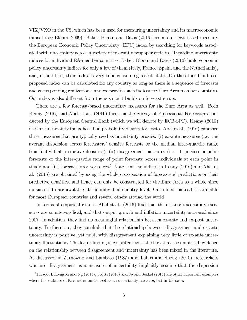
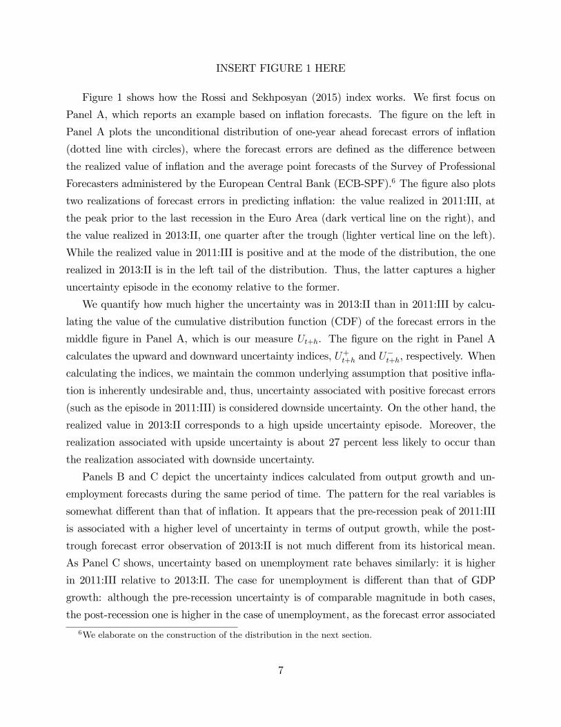
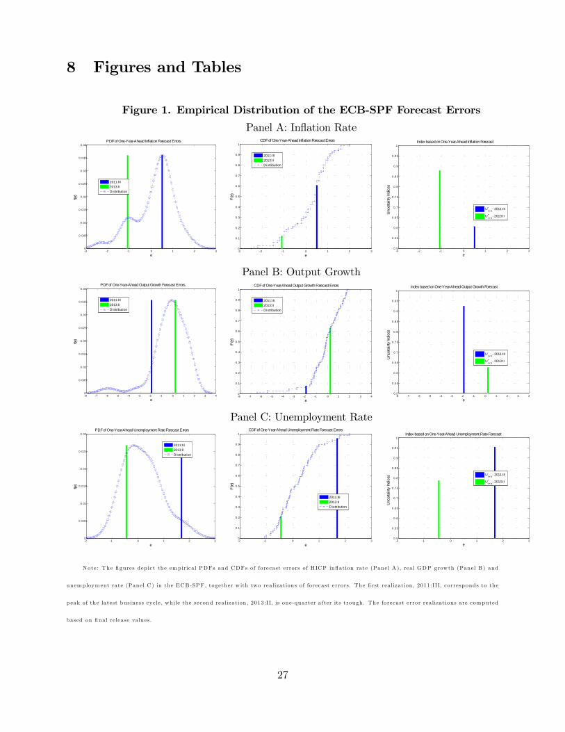
Figure 1 shows how the Rossi and Sekhposyan (2015) index works. We �rst focus on

Panel A, which reports an example based on in�ation forecasts. The �gure on the left in

Panel A plots the unconditional distribution of one-year ahead forecast errors of in�ation

(dotted line with circles), where the forecast errors are de�ned as the di¤erence between

the realized value of in�ation and the average point forecasts of the Survey of Professional

Forecasters administered by the European Central Bank (ECB-SPF).6 The �gure also plots

two realizations of forecast errors in predicting in�ation: the value realized in 2011:III, at

the peak prior to the last recession in the Euro Area (dark vertical line on the right), and

the value realized in 2013:II, one quarter after the trough (lighter vertical line on the left).

While the realized value in 2011:III is positive and at the mode of the distribution, the one

realized in 2013:II is in the left tail of the distribution. Thus, the latter captures a higher

uncertainty episode in the economy relative to the former.

We quantify how much higher the uncertainty was in 2013:II than in 2011:III by calcu-

lating the value of the cumulative distribution function (CDF) of the forecast errors in the

middle �gure in Panel A, which is our measure Ut+h. The �gure on the right in Panel A

calculates the upward and downward uncertainty indices, U+t+h and U�t+h, respectively. When

calculating the indices, we maintain the common underlying assumption that positive in�a-

tion is inherently undesirable and, thus, uncertainty associated with positive forecast errors

(such as the episode in 2011:III) is considered downside uncertainty. On the other hand, the

realized value in 2013:II corresponds to a high upside uncertainty episode. Moreover, the

realization associated with upside uncertainty is about 27 percent less likely to occur than

the realization associated with downside uncertainty.

Panels B and C depict the uncertainty indices calculated from output growth and un-

employment forecasts during the same period of time. The pattern for the real variables is

somewhat di¤erent than that of in�ation. It appears that the pre-recession peak of 2011:III

is associated with a higher level of uncertainty in terms of output growth, while the post-

trough forecast error observation of 2013:II is not much di¤erent from its historical mean.

As Panel C shows, uncertainty based on unemployment rate behaves similarly: it is higher

in 2011:III relative to 2013:II. The case for unemployment is di¤erent than that of GDP

growth: although the pre-recession uncertainty is of comparable magnitude in both cases,

the post-recession one is higher in the case of unemployment, as the forecast error associated

6We elaborate on the construction of the distribution in the next section.

7

with the forecast made in 2013:II is about 1/4-th less likely than that of GDP growth.

3 The Euro Area Uncertainty Indices

We construct the overall as well as the upside and downside uncertainty indices for the Euro

Area based on the point forecasts from the Survey of Professional Forecasters administered

by the European Central Bank. The ECB Survey of Professional Forecasters (ECB-SPF)

is a quarterly survey of expectations for several target variables and for a variety of short,

medium and long term horizons. It collects professional forecasters�expectations of in�ation

(year on year percentage change of the Harmonised Index of Consumer Prices), real GDP

growth (year on year percentage change of real GDP) and unemployment rates (de�ned as

the number of unemployed between 15 � in some countries 16 �and 74 years of age as a

percentage of the labor force) in the Euro Area. The ECB-SPF adapts to the changing

composition of the Euro Area, i.e. accounting for the new member countries as they join the

currency union.

Our uncertainty index relies on the average point forecasts across the cross section of

individual forecasters. In order to construct the unconditional densities of forecast errors,

we use forecasts from 1999:I to 2015:II for in�ation and unemployment rate and 1999:I

to 2015:III for output growth.7 Further, in the benchmark speci�cation, we use the �nal

release of the data as the realization when calculating the forecast errors. However, we also

investigate the behavior of our indices when the �rst release of the data is used instead.

It should be noted that the ECB-SPF dataset provides both �xed and moving horizon

forecasts. In other words, each quarter the forecasters are asked to provide forecasts for

speci�c calendar years (moving horizon forecasts) as well as for one, two and �ve year ahead

(�xed horizon forecasts). The di¤erence between the �xed and moving horizon forecasts is

as follows.

A moving horizon forecast is a forecast where, in January of 2013 (i.e. the �rst quarter),

the forecasters are asked to provide their expectations for calendar years 2013, 2014 and 2015.

Then, they are asked the same information in April of 2013 (i.e. the second quarter). If we

were to use the current year forecasts they provide in the �rst two quarters of 2013, we would

compare forecasts whose horizons are changing: the forecasts made in April would have one

quarter of uncertainty that has already been resolved relative to the January forecasts.

7The data publication calendar and the target forecast horizons enable us to use one more observation

for output growth forecasts.

8

A �xed horizon forecast, instead, is one where, for example, in January 2013 forecasters

are requested projections for December 2013 and, subsequently, in April 2013 they are asked

their projections for March 2014. We choose to work with the �xed horizon forecasts since

they are not a¤ected by the resolution of uncertainty over time. The available �xed horizon

ECB-SPF forecasts measure expectations for one-, two- and �ve-years ahead of the period

for which the most up-to-date o¢ cial data releases are available; we focus on forecasts of all

the macroeconomic variables at the one-year-ahead �xed horizon, since it makes our results

more comparable with those in Rossi and Sekhposyan (2015).

There are a few intricacies associated with the ECB-SPF. First, the survey also provides

conditional density forecasts where the respondents provide their probability assessments

about particular economic outcomes. This could be a natural choice for measuring uncer-

tainty in the Euro Area (as some of the literature discussion in the introduction does).8

Instead, we focus on the unconditional densities based on average point forecasts across the

forecasters. Our choice is done for consistency, as our ultimate goal is to provide country-

speci�c uncertainty indices for a wide variety of countries (discussed in Section 4): for the

majority of the countries we consider, neither densities nor individual forecasts are available.

Hence, it would be impossible to calculate measures of uncertainty based on predictive den-

sities or other measures of central tendencies extracted from the cross-section of forecasts.

Our measure of uncertainty based on the point forecast, on the other hand, can be easily ob-

tained. Moreover, Clements (2016) points out that unconditional densities of point forecasts

appear to be more informative than conditional predictive densities, at least in the context

of the US Survey of Professional Forecasters.

In the ECB-SPF, the forecast horizon also has variable-speci�c peculiarities. Namely,

the one-year-ahead forecasts refer to a one-year-ahead time period from the date of the

last realization in the information set of both the researchers and the public. As such,

though the forecasts of output growth, in�ation as well as the unemployment rate are one-

year-ahead, they pertain to di¤erent time periods in the year. As discussed in Genre et

al. (2013), the �one-year ahead forecast is actually around six-to-eight months ahead for

GDP growth, eleven months ahead for the unemployment rate and twelve months ahead for

HICP in�ation.�In order to match the forecast horizons accurately, we go through the ECB

SPF�s individual forecast dataset to elicit the speci�c one-year-ahead horizon for which the

8For a careful treatment of the ECB-SPF predictive densities in the context of understanding forecasters�

learning mechanisms see Manzan (2016).

9

forecasters are asked to provide predictions.9

As mentioned earlier, in the benchmark speci�cation the forecasts are evaluated against

the �nal release of the data. This is done in order to be consistent with the country-speci�c

indices, for most of which no real-time data vintages of realizations are available. For the

Euro Area, the last vintage of the data used as a �nal release data belongs to June 1,

2016. The last observations in the series for output growth, in�ation and unemployment

rate respectively are 2016Q1, May 2016 and April 2016. When considering the robustness of

the results to real-time data, we use the �rst available realization from the real time database

for the Euro Area (as discussed in Giannone et al., 2012).10

3.1 Variable-speci�c Uncertainty Indices for the Euro Area

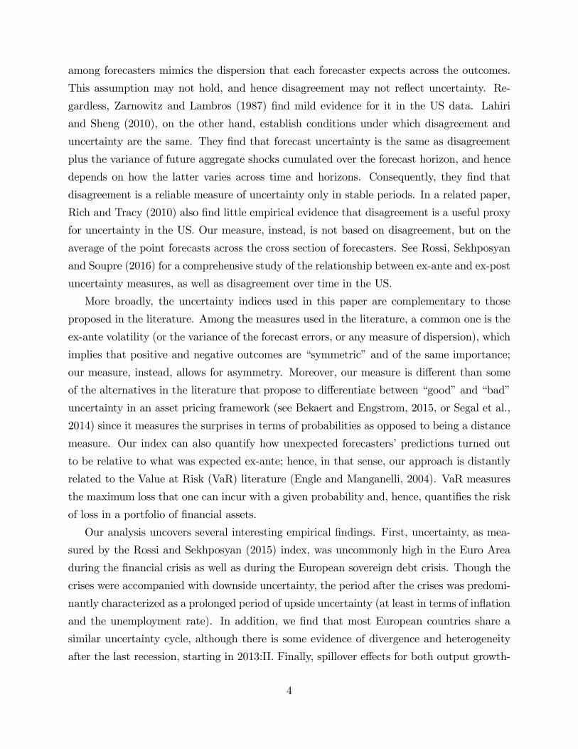
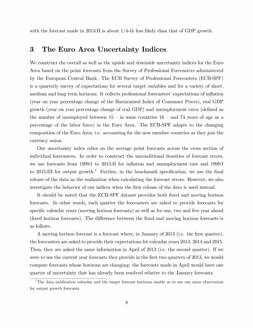
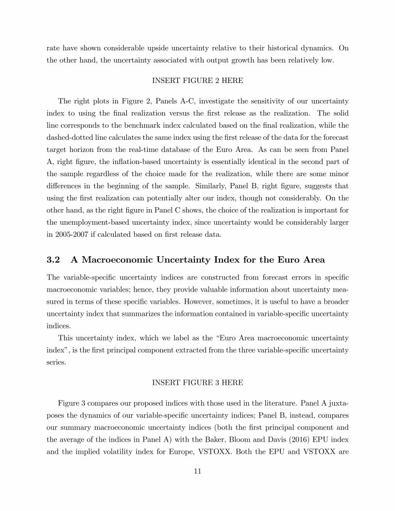
Figure 2 plots Rossi and Sekhposyan�s (2015, hereafter labeled RS) overall uncertainty index

U�t+h, as well as the downside uncertainty (�Downside UC�, U�t+h) and upside uncertainty

(�Upside UC�, U+t+h) indices extracted from the distribution of the forecasts errors of in�a-

tion, output growth and the unemployment rate. The �gure also plots the CEPR recession

dates, determined by the Euro Area Business Cycle Dating Committee (shaded areas).11

Common wisdom associates the few years after 2007 with high uncertainty, due to the �nan-

cial crisis in 2007-2009 and the European sovereign debt crisis in 2010-2012. It is reassuring

that our uncertainty index captures such episodes (as shown in the left panels in Figure 2).

In fact, the left �gures in Panels B and C show that the downside uncertainty in the real side

of the economy, namely output growth and the unemployment rate, spikes during recessions;

however, there is also an episode of downside uncertainty in the early 2000s. It is worth

noting that, after the last recession in the Euro Area, both in�ation and the unemployment

9The European SPF dataset for the individual as well as aggregate forecasts are available at:

http://www.ecb.europa.eu/stats/prices/indic/forecast/html/index.en.html

To appreciate the importance of this point, consider again the January 2013 survey. In the �rst quarter of

2013, the one-year-ahead forecast of in�ation is for December 2013, while that of the unemployment rate is

for November 2013, and the GDP growth prediction for 2013:III. In order to properly evaluate the forecasts,

we use year-over-year growth rates of in�ation and GDP growth matched to the speci�c forecast target date.

For instance, the GDP growth rate forecast from January 2013 (quarter I) is matched to the realization

corresponding to real GDP growth from 2012:III to 2013:III. Since the unemployment rate is forecasted in

levels, we use the realization associated with the target date.10The real-time database as well as the instructions on how to download the data are available at:

https://sdw.ecb.europa.eu/browseExplanation.do?node=9689716.11The dates are provided at: http://cepr.org/content/euro-area-business-cycle-dating-committee.

10

rate have shown considerable upside uncertainty relative to their historical dynamics. On

the other hand, the uncertainty associated with output growth has been relatively low.

INSERT FIGURE 2 HERE

The right plots in Figure 2, Panels A-C, investigate the sensitivity of our uncertainty

index to using the �nal realization versus the �rst release as the realization. The solid

line corresponds to the benchmark index calculated based on the �nal realization, while the

dashed-dotted line calculates the same index using the �rst release of the data for the forecast

target horizon from the real-time database of the Euro Area. As can be seen from Panel

A, right �gure, the in�ation-based uncertainty is essentially identical in the second part of

the sample regardless of the choice made for the realization, while there are some minor

di¤erences in the beginning of the sample. Similarly, Panel B, right �gure, suggests that

using the �rst realization can potentially alter our index, though not considerably. On the

other hand, as the right �gure in Panel C shows, the choice of the realization is important for

the unemployment-based uncertainty index, since uncertainty would be considerably larger

in 2005-2007 if calculated based on �rst release data.

3.2 A Macroeconomic Uncertainty Index for the Euro Area

The variable-speci�c uncertainty indices are constructed from forecast errors in speci�c

macroeconomic variables; hence, they provide valuable information about uncertainty mea-

sured in terms of these speci�c variables. However, sometimes, it is useful to have a broader

uncertainty index that summarizes the information contained in variable-speci�c uncertainty

indices.

This uncertainty index, which we label as the �Euro Area macroeconomic uncertainty

index�, is the �rst principal component extracted from the three variable-speci�c uncertainty

series.

INSERT FIGURE 3 HERE

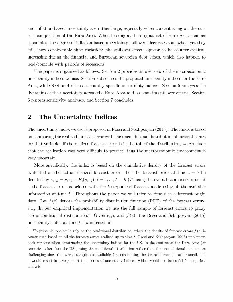
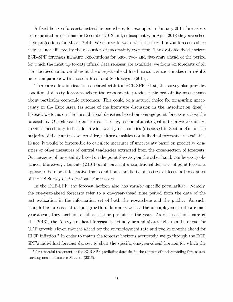
Figure 3 compares our proposed indices with those used in the literature. Panel A juxta-

poses the dynamics of our variable-speci�c uncertainty indices; Panel B, instead, compares

our summary macroeconomic uncertainty indices (both the �rst principal component and

the average of the indices in Panel A) with the Baker, Bloom and Davis (2016) EPU index

and the implied volatility index for Europe, VSTOXX. Both the EPU and VSTOXX are

11

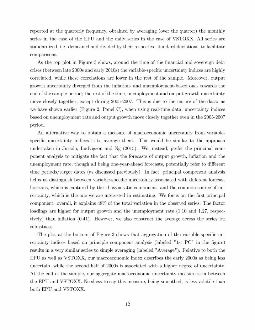
reported at the quarterly frequency, obtained by averaging (over the quarter) the monthly

series in the case of the EPU and the daily series in the case of VSTOXX. All series are

standardized, i.e. demeaned and divided by their respective standard deviations, to facilitate

comparisons.

As the top plot in Figure 3 shows, around the time of the �nancial and sovereign debt

crises (between late 2000s and early 2010s) the variable-speci�c uncertainty indices are highly

correlated, while these correlations are lower in the rest of the sample. Moreover, output

growth uncertainty diverged from the in�ation- and unemployment-based ones towards the

end of the sample period; the rest of the time, unemployment and output growth uncertainty

move closely together, except during 2005-2007. This is due to the nature of the data: as

we have shown earlier (Figure 2, Panel C), when using real-time data, uncertainty indices

based on unemployment rate and output growth move closely together even in the 2005-2007

period.

An alternative way to obtain a measure of macroeconomic uncertainty from variable-

speci�c uncertainty indices is to average them. This would be similar to the approach

undertaken in Jurado, Ludvigson and Ng (2015). We, instead, prefer the principal com-

ponent analysis to mitigate the fact that the forecasts of output growth, in�ation and the

unemployment rate, though all being one-year-ahead forecasts, potentially refer to di¤erent

time periods/target dates (as discussed previously). In fact, principal component analysis

helps us distinguish between variable-speci�c uncertainty associated with di¤erent forecast

horizons, which is captured by the idiosyncratic component, and the common source of un-

certainty, which is the one we are interested in estimating. We focus on the �rst principal

component: overall, it explains 48% of the total variation in the observed series. The factor

loadings are higher for output growth and the unemployment rate (1.10 and 1.27, respec-

tively) than in�ation (0.41). However, we also construct the average across the series for

robustness.

The plot at the bottom of Figure 3 shows that aggregation of the variable-speci�c un-

certainty indices based on principle component analysis (labeled "1st PC" in the �gure)

results in a very similar series to simple averaging (labeled "Average"). Relative to both the

EPU as well as VSTOXX, our macroeconomic index describes the early 2000s as being less

uncertain, while the second half of 2000s is associated with a higher degree of uncertainty.

At the end of the sample, our aggregate macroeconomic uncertainty measure is in between

the EPU and VSTOXX. Needless to say this measure, being smoothed, is less volatile than

both EPU and VSTOXX.

12

INSERT TABLE 1 HERE

Table 1 reports correlations between the various variable-speci�c indices, the macro-

economic uncertainty index, the EPU and VSTOXX. As the table indicates, uncertainty

indices based on real variables (output growth and employment) are highly correlated with

each other, as well as with the principal component summary measure (which loads heavily

on them). The correlation of the real uncertainty measures with that of in�ation uncertainty

is somewhat smaller. Moreover, it appears that our macroeconomic index is more correlated

with VSTOXX than the EPU, though in absolute value these correlations are small.

4 Individual Euro Area Member Country-Speci�c Un-

certainty Indices

One of the contributions of this paper is to provide individual Euro Area country-speci�c

uncertainty indices based on our measure. Baker, Bloom and Davis (2016) build economic

policy uncertainty indices for several Euro Area countries, such as Germany, Italy, France,

Spain and the Netherlands. However, their index is very time-consuming to calculate, and

it is not available for a wide variety of countries. On the other hand, our proposed index can

be calculated for any country as long as there is a sequence of forecasts and corresponding

realizations. The Euro Area countries for which we have constructed the indices, with the

respective periods for which time series of uncertainty indices are available, are listed in

Table 2. The time series are available on our webpages. It is also noteworthy that Table

2 lists the current composition of the Euro Area, which changed over time. For instance,

Greece joined in 2001, Slovenia in 2007, Slovakia in 2009, Estonia in 2011, Latvia in 2014

and Lithuania in 2015. We provide the indices for seventeen out of the current nineteen

Euro Area member countries. We have no available data for Malta and Luxemburg.

INSERT TABLE 2 HERE

The uncertainty indices for the individual countries are based on Consensus Economics

forecast errors. The forecasts generally start on 1990:M1, although for some countries they

start later. Moreover, the frequency of the forecasts change over time. For instance, for

Eastern Europe, the survey was conducted every two months between May 1998 and April

2007 and monthly thereafter. For the remaining countries, the survey provides monthly

point forecasts (which are the average across forecasters). The realizations are from Haver

13

Analytics and correspond to �nal release values. The data sources we used were chosen to

collect the largest possible sample of countries and time periods.

By construction, Consensus Economics forecasts are �xed-event forecasts: data are col-

lected monthly, but forecasts refer to the average rate of growth of GDP and CPI in�ation

over either the current year or the next calendar year. Being �xed-event forecasts, their

horizon changes over the year (as discussed in Section 3). We construct monthly �xed-

horizon forecast using the method proposed by Dovern et al. (2012). Dovern et al. (2012)

propose taking weighted averages of the current-year and next-year forecasts. For example,

in the case of GDP data, for each month the survey contains a pair of ��xed-event� fore-

casts for the current-year, which we label bfFEt+kjt, and for the following year, which we labelbfFEt+k+12jt. The twelve�month-ahead (�xed-horizon) forecast at time t is the average of thetwo �xed-event forecasts using weights that are proportional to their share of overlap with

the forecast horizon. Let k denote the number of months from time t until the end of the

year, k = 1; 2; 3; 4; :::; 12; then the �xed horizon forecast is k12bfFEt+kjt + 12�k

12bfFEt+k+12jt.12 We use

a similar procedure for in�ation.13

As mentioned, the realizations are the seasonally adjusted in�ation and output growth

values taken from Haver Analytics. The GDP growth data is available at the quarterly

frequency, while in�ation is monthly. In order to construct the forecast errors, we �rst

aggregate the �xed-horizon monthly output growth forecasts into quarterly series, and then

compare them to the quarterly realization of output growth. For in�ation, we construct both

monthly and quarterly uncertainty indices. To make the indices comparable to the ECB-

SPF Euro Area uncertainty indices, in this section we only report the quarterly indices;

a discussion of the monthly in�ation-based indices is provided in our robustness section.

We use the quarterly averages of the monthly realizations and the �xed-horizon-forecasts to

obtain the quarterly forecast errors.14

12E.g.: in month one, k = 12, while in month twelve, k = 1. An alternative procedure to construct �xed-

horizon forecasts from �xed-event ones is developed by Knueppel and Vladu (2016). Their procedure gives

optimal weights that minimize the mean squared forecast error loss function of the �xed-horizon forecast.

For the purposes of our index, which is based on the unconditional distribution of the forecast errors, this

alternative weighting results in very similar uncertainty indices. However, if one were to construct uncertainty

indices based on the conditional distributions, the di¤erence could be non-negligible.13In the sample periods where forecasts are available only every two months, the current year and next

year forecasts are weighted based on the adjusted formula: k6bfFEt+kjt + 6�k

6bfFEt+k+6jt, where k = 1; 2; :::; 6:

14The survey forecasts as well as the realizations for the countries start potentially at di¤erent points

in time. If we miss some observations for the three months of the quarter for either the forecasts or the

realizations, we construct the quarterly average based on the available observations. This situation occurs

14

The timing of the surveys relative to the realizations is worth a separate discussion.

When the survey takes place, typically only the past value of the realization is available.

Thus, in the �rst month of the year, when the forecasts are obtained, the realizations for

the current year have not been published yet. Following the procedure that is typically used

for the ECB-SPF, which faces a similar problem, we calculate the realizations as one-year-

ahead growth rates from the last data release that was available to the forecasters at the

time they made their forecasts. For instance, the realization we associate to the quarterly

one-year-ahead forecast in the �rst quarter of the year captures GDP growth between the

fourth quarter of the current year relative to the fourth quarter of the previous year.

INSERT FIGURES 4 AND 5 HERE

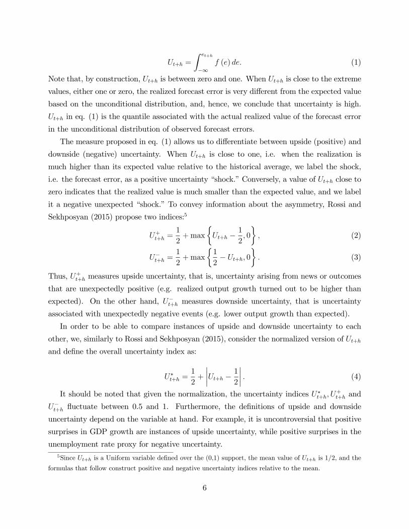
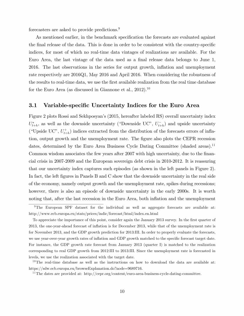
Figures 4 and 5 depict the upside and downside uncertainty indices for the individual Euro

Area countries in our dataset. Figure 4 shows the overall macroeconomic uncertainty index

based on GDP growth forecast errors, while Figure 5 focuses on the in�ation uncertainty

index. The shaded areas highlight Euro Area-wide recessions identi�ed by the CEPR business

cycle dating committee, rather than country-speci�c recession dates which are not available.

Figure 4 shows that most European countries share a similar overall macroeconomic un-

certainty cycle, as the downside uncertainty index tracks closely the recession dates. How-

ever, the timing and magnitude di¤er somewhat across countries. Comparing Figure 4 with

Figure 2, Panel B, the behavior of the individual Euro Area countries is also similar to

the behavior of the uncertainty indices in the Euro Area. There is evidence of divergence

towards the end of the sample, though, as some countries experienced upside uncertainty

(e.g. Ireland, Slovenia, Slovakia, Spain, etc.), while others experienced downside uncertainty

(Austria, Greece, Latvia, Lithuania, etc.).

Figure 5 shows that in�ation uncertainty is more homogeneous across countries relative

to output growth uncertainty. There is evidence of upside uncertainty in most countries

during the 1990s, which disappears in the 2000s. The latest part of the sample can still

be described by upside uncertainty across the board. Considering the overlapping period

where the Euro Area (reported in Figure 2, Panel A) and the individual member country

uncertainty indices are both available, their behavior is very similar.

only in the case of Eastern European forecasts during the sample period where the forecasts are every two

months rather than monthly.

15

5 Spillover E¤ects of Uncertainty in the Euro Area

The previous section described country-speci�c uncertainty indices based on in�ation and

output growth forecast errors and analyzed their relationship to the broader Euro Area

index by visual inspection. Here we delve in more details. First, we compare the common

component of the country-speci�c indices to the ECB-SPF Euro Area one. Second, we

investigate the heterogeneity across the Euro Area countries by looking at correlations over

the business cycle. Third, we formally investigate the spillovers of uncertainty across the

countries and over time via a network analysis.

5.1 The ECB-SPF Euro Area Uncertainty Index versus Individual

Countries�Uncertainty Index Aggregates

In this sub-section, we compare the Euro Area uncertainty indices constructed based on the

ECB-SPF forecasts to aggregate country-speci�c indices extracted from the Consensus Eco-

nomics survey-based country-speci�c indices. The aggregate uncertainty indices constructed

form the individual countries� indices are the principal component and the cross country

average. Note that the latter are based on the current Euro Area composition, while the

ECB-SPF Euro Area uncertainty indices are based on the changing composition of the Euro

Area instead. We focus our analysis on the sub-sample where all the indices overlap.

INSERT FIGURE 6

The left panel in Figure 6 depicts the indices for output growth, and the right panel

depicts the indices for in�ation. The panels show that the average of country-speci�c un-

certainty indices behaves similarly to the �rst principal component; thus, it does not matter

how we aggregate the individual countries�uncertainty indices to obtain an aggregate index.

However, it matters whether we consider the aggregate index based on individual countries�

indices or the ECB-SPF Euro Area aggregate index, as they turn out to be quite di¤erent.

In fact, in the case of GDP growth, the ECB-SPF-based measure oscillates roughly around

the cross-country average; on the other hand, in the case of in�ation, the cross-country av-

erage identi�es a higher level of uncertainty prior to 2007. It is worth noting that the two

measures have diverged in the recent period: the ECB-SPF Euro Area aggregate suggests a

lower output growth uncertainty than the cross-country average, while it is the opposite for

16

in�ation.15 The correlation coe¢ cient between the ECB-SPF Euro Area aggregate and the

cross-country averages is 0.62 for output growth and 0.68 for in�ation.

5.2 Heterogeneity in Euro-Area Uncertainty

Figure 7 shows the average uncertainty in the Euro Area and its member economies from

1999:I till 2013:I (Panel A) and 2013:II-2015:II (Panel B). The pictures in Panel A show

that the average uncertainty has been more or less homogeneous in the Euro Area up to

the end of the last recession. However, as Panel B suggests, after the trough of the last

recession the heterogeneity has increased. As shown in the left �gure, GDP growth-based

uncertainty in Belgium, France, Germany and Slovakia appears to be lower than that based

on the ECB-SPF Euro Area, while it is higher in other countries, especially Ireland, Slovenia

and Spain. On the other hand, in�ation uncertainty in general appears to be higher relative

to the GDP-based uncertainty. As discussed previously, the ECB-SPF Euro Area aggregate

in�ation uncertainty is higher than the cross-section average; as evident from Figure 7, it

is also higher than that of any of its members. This emphasizes the divergence between

the Euro Area and its members in terms of in�ation expectations and outcomes after the

crises. This might be indicative of the fact that though the forecasters are more certain

about country-speci�c outcomes, they are more uncertain about the Euro Area wide policy,

which is re�ected in an increased area-wide uncertainty. Moreover, countries with high GDP

growth-based uncertainty do not necessarily have high in�ation-based uncertainty.

INSERT FIGURE 715Besides the �xed country-composition of the aggregate index that is imposed when constructing the

aggregate index using individual countries�indices versus the changing composition embedded in the ECB-

SPF, other potential reasons for the divergence between the two measures could be the fact that they come

from di¤erent surveys, with potentially di¤erent participants. Moreover, it is possible that the ECB-SPF

participants weigh the country-speci�c data di¤erently than our averaging or principal component extraction

imply. In addition, though the two sets of forecasts are compared to each other as of the forecast origin

dates, their target dates vary. As discussed earlier, the target date for the weighted Consensus forecasts in

the �rst quarter would be the year-over-year growth from the fourth quarter of the last year to the fourth

quarter of the current year. On the other hand, that of GDP growth-based uncertainty from the ECB-SPF

is based on the growth from quarter 3 of the previous year to quarter 3 of the current year. This, if anything,

would put a lower bound on the leading properties of country-speci�c uncertainty indices relative to the

Euro Area aggregate. For in�ation, the target periods are the same, so the di¤erential in the target dates

should be irrelevant.

17

Tables 3 and 4 display correlations of the country-speci�c output growth (Table 3) and

in�ation (Table 4) uncertainty indices with that of the corresponding ECB-SPF Euro Area

aggregate.16 When k = 0, the table reports contemporaneous correlations. For each country,

we highlight in bold the contemporaneous correlation as well as any correlation higher (in

absolute value) than the corresponding contemporaneous correlation. According to Table 3,

GDP growth-based uncertainty leads that of the Euro Area for economies such as Austria,

Belgium, Finland, France, Germany, Italy, the Netherlands and, to a lesser degree, Slovakia.

The largest contemporaneous correlations are reported for Germany and Italy. This �nding

is not surprising, as Germany, France and Italy are among the largest countries in the Euro

Area in terms of GDP. The picture is less clear in the case of in�ation: it appears that, for

most countries, in�ation uncertainty is coincidental with the ECB-SPF Euro Area aggregate;

the largest contemporaneous correlations are those of Belgium and Spain.

INSERT TABLES 3 AND 4 HERE

5.3 Uncertainty Spillovers in the Euro Area: a Network Approach

Lastly, we study the spillover of uncertainty in the Euro Area. In order to do so we rely on

the methodology proposed by Diebold and Yilmaz (2009) and implement it in the robust

framework of Klößner and Wagner (2013).17 More speci�cally, we study the spillovers in a

Vector Autoregression (VAR) framework and propose an uncertainty spillover index. The

spillover index accounts for the total share of uncertainty shocks of non-domestic origin across

all the countries. The analysis is not intended to give a causal interpretation of the spillovers

of uncertainty in the Euro Area, but rather provides a measure of pairwise directional and

total inter-connectedness.

Borrowing some of the notation from Klößner and Wagner (2013), let Yt be an N di-

mensional vector of uncertainty indices for the N countries in the sample and consider the

standard VAR(p): Yt = �1Yt�1 + �2Yt�2 + ::: + �pYt�p + "t, where "t is a white noise with

a variance-covariance matrix of ", while f�igpi=1 are N � N coe¢ cients summarizing the

dynamic behavior of the system. Given the maintained assumption of stationarity of the

VAR, the MA(1) representation is: Yt = "t + A1"t�2 + A2"t�2 + :::. The spillover ef-

fects are derived from the forecast error decomposition. The h-step-ahead forecast error is

16Note that we do not report the correlations for Cyprus as it does not have enough available observations

to precisely estimate correlations for leads and lags up to order four.17The algorithm is implemented with the fastsSOM package in R, see Klößner and Wagner (2016).

18

et+h = Yt+h�Yt+hjt = "t+h+A1"t+h�1+A2"t+h�2+ :::Ah�1"t+1: The forecast error covariancematrix, consequently, can be written as e;h = �h�1i=0Ai"A

0i, where A0 is the identity matrix.

Diebold and Yilmaz (2009) choose to work with the Cholesky factorization of ". If L is the

Cholesky factor of ", such that LL0= ", then country k�s contribution to country j�s fore-

cast error variance can be written as��h�1i=0

��Nk=1 (AiL)jk (AiL)

0

jk

���1�h�1i=0 (AiL)jk (AiL)

0

jk,

and the uncertainty spillover index (USOI) is de�ned as:

USOI = 100�Nj=1

�h�1i=0

��Nk=1;k 6=j (AiL)jk (AiL)

0

jk

��h�1i=0

��Nk=1 (AiL)jk (AiL)

0

jk

� (5)

The Cholesky decomposition is not order invariant and the analysis is not structural,

that is, there is no preferred Cholesky rotation over the others based on economic theory;

thus, one would have to take into account multiple Cholesky rotations (precisely N !) in

a robustness analysis. We implement Klößner and Wagner�s (2013) algorithm to perform

forecast error variance decomposition analysis for all possible Cholesky rotations and report

the average over all of them. Diebold and Yilmaz (2009), on the other hand, only veri�ed

the robustness of their analysis to a few set of alternative Cholesky rotations.

Our exercise is similar to that in Klößner and Sekkel (2014), although we focus on the

Euro Area and use the indices proposed in Rossi and Sekhposyan (2015). Klößner and

Sekkel (2014), instead, study spillovers of the Baker et al. (2016) index for countries such

as Canada, France, Germany, Italy, US and the UK. They �nd that between January 1997

and September 2013 the spillover index among the set of these six developed countries was

approximately 27%. Moreover, they �nd time-variation in the spillover e¤ects; the spillovers

are countercyclical: they were relatively high until 2006, they then decreased and then spiked

again around 2008 due to the �nancial crisis and associated high policy uncertainty. They

also �nd evidence that the spillovers have been declining since then: at the end of their

sample, their level was roughly the same as before 2008. Furthermore, they �nd that some

countries (such as the US, the UK and France) have been net �exporters� of uncertainty,

while the rest have on average been net �importers��although, for some countries, the role

has reversed over time.

We perform a similar type of analysis, with the objective of understanding the spillover

e¤ects in the Euro Area. We report the results for output growth-based uncertainty in Table

5 and those for in�ation-based uncertainty in Table 6. Our empirical results are based on es-

timating VARs with two lags for sixteen Euro Area countries (excluding Cyprus, Luxemburg

and Malta from the current list of members) and performing the variance decomposition at

19

the two-year-ahead forecast horizon (h = 8). We also include the Euro Area aggregate in our

analysis, which could capture some of the spillovers from the current Euro Area countries

that are not accounted for in the Euro Area aggregate due to the changing nature of its

membership.

As Table 5 shows, the spillover e¤ects for output-growth-based uncertainty in the Euro

Area are high, about 74%. Moreover, some of the countries, namely Austria, Belgium,

France, Latvia, Portugal, Slovakia, Slovenia, Spain and the Netherlands have been on average

uncertainty �exporters,�as the net contribution (�To�- �From�) of the uncertainty in these

countries is positive (marked in bold in the row labeled �Net�). The three countries with

the highest spillover e¤ects are Austria, Belgium and Slovakia: this is certainly surprising

given that these countries are relatively small members of the Euro Area. It is interesting

to note that the �importers�of uncertainty are Finland and Ireland, while the Euro Area as

an aggregate also turns out to be a net importer of uncertainty.

The case of in�ation-based uncertainty, shown in Table 6, is somewhat di¤erent. In

this case, the Euro Area, as well as Austria, Belgium, Estonia, France, Italy, Portugal and

Spain, turn out to be uncertainty �exporters.�The overall spillover e¤ects are also fairly

high, amounting to about 78%: in particular, it is interesting to note that they are much

higher (2.5-2.7 times) than those detected by Klößner and Sekkel (2014). According to our

spillover index, only about one quarter of the uncertainty in the Euro Area is of idiosyncratic

country-speci�c nature, while the rest derives from the inter-connectedness, which transmits

the uncertainty.

INSERT TABLES 5 AND 6 HERE

When we condition on the type of uncertainty, the picture changes somewhat. Table

7 shows the per country net contribution of uncertainty, together with the spillover index

for both upside and downside uncertainty. When the upside and downside uncertainties are

considered separately, the overall spillover index jumps by about 10 percentage points: in the

case of output growth, upside and downside uncertainty rise to 84% and 85%, respectively;

in the case of in�ation, it increases to 87% (relative to 78%, the value we estimated when

we did not distinguish between the sources of the uncertainty).

INSERT TABLE 7 HERE

Moreover, which countries are exporters or importers of uncertainty also changes. Ex-

porter countries are marked in bold in Table 7. When we look at output growth-based

20

uncertainty (columns 2 and 3), now Austria, Belgium, Germany, Lithuania, Portugal and

the Netherlands are �exporters� of upside uncertainty, while Belgium, Estonia, Finland,

France, Germany, Ireland and Portugal �export�downside uncertainty. It should be noted

that, Germany, which was a net �importer�of uncertainty, becomes an �exporter�when we

take into account the conditional source of the uncertainty. Belgium, Germany and Portu-

gal appear to be �exporters�for both kinds of output-growth based uncertainties. For the

in�ation-based uncertainty (columns 4 and 5), the Euro Area, France, Germany and Spain

turn out to be both �exporters�and �importers�of uncertainty; Austria, Estonia, Greece and

Italy turn out to be �exporters�of downside uncertainty, while Ireland, Portugal, Slovakia

and Slovenia turn out to be �exporters�of upside uncertainty.

Our results are surprising, since, during the period of the sovereign debt crises, one would

have expected Greece, Ireland, Italy, Portugal and Spain to be exporters of uncertainty, as

these countries are the ones whose yields increased to compensate for the risk associated with

either budgetary and/or banking problems. However, in our analysis Greece, for instance,

does not come out as a main source of uncertainty across the Euro Area. In fact, it becomes

an �exporter�only of downside in�ation-based uncertainty. This is the because our index is

di¤erent from those considered in the literature: we measure uncertainty as the likelihood of

unexpected outcomes (that is, we control for conditional expectations), while the measures

such as the EPU or VSTOXX are unconditional. This is crucial since unconditionally (or

ex-ante) the uncertainty associated with the performance of the Greek government debt (and

thus the Greek economy) might have been high; however, after controlling for expectations,

the surprises and their associated uncertainty might not have been so high, and thus their

spillover e¤ects not as large.

6 Sensitivity Analysis

In this section, we �rst investigate the robustness of our results to monthly in�ation-based

uncertainty indices. Namely, we show monthly indices for the eleven countries in the Euro

Area (the ten original members and Greece). In fact, while output growth-based uncer-

tainty indices are, by construction, quarterly, since real GDP is only provided quarterly for

the majority of the countries, country-speci�c in�ation-based uncertainty indices can be con-

structed at the monthly frequency.18 Second, we consider spillovers of uncertainty across the

18In fact, we previously constructed monthly indices, and then aggregated them to the quarterly frequency

to make them comparable to the output growth-based indices as well as the aggregate ECB-SPF Euro Area

21

European countries. Lastly, since monthly indices are available with a much larger number

of time series observations, they enable us to study the evolution of spillovers over time,

which we were unable to do in quarterly data given their small sample size.

Figure 8 shows monthly in�ation-based uncertainty indices for a set of European countries

which includes the ten original members of the Euro Area (minus Luxemburg, for which we

have no data) and Greece. We do not consider Eastern European countries such as Estonia,

Latvia, Lithuania, Slovakia and Slovenia since forecasts are only available every two months

in the beginning of the sample for these countries and thus the sample is too short to study

the evolution of spillovers over time. As the �gure shows, monthly indices are broadly

similar to the quarterly ones reported in Figure 5. The only noticeable di¤erence is the

volatility of the indices: monthly indices are more volatile than quarterly ones, although our

conclusions regarding upside and downside uncertainty and the identi�cation of periods of

high uncertainty are the same regardless of the frequency.

INSERT FIGURE 8 HERE

Table 8 reports the analysis of spillover e¤ects for the monthly in�ation-based uncertainty

index in the eleven Euro Area countries.19 As before, the VAR includes 2 lags and the

forecast horizon equals 24 month in order to facilitate comparison with previous results.

The spillover index decreases to 45%; thus, in this di¤erent set of countries, slightly more

than half of uncertainty volatility can be explained by idiosyncratic uncertainty, while about

45% is due to spillovers from other countries. Moreover, Belgium, Germany, Greece and

Spain turn out to be, on average, uncertainty �exporters,�while the rest of the countries

are, on average, uncertainty �importers.�This is in contrast to the results reported in Table

6: from the set of the countries classi�ed as �exporters�, only Belgium and Spain remain

classi�ed as such. Our sensitivity results show that not only the overall spillover index, but

also the classi�cation of countries as uncertainty �exporters�and �importers�clearly depends

on the network: a larger network decreases the role of idiosyncratic shocks and increases the

importance of spillovers.

INSERT TABLE 8 HERE

in�ation-based ones.19Recall that the network is smaller in this analysis than that considered in the main empirical exercise, as

here we only consider eleven countries instead of the nineteen in our main empirical analysis with quarterly

data.

22

Lastly, Figure 9 shows the spillover e¤ects over time, as well as the net contribution of

each country to the overall uncertainty. The statistics are calculated on a 60 month rolling

window. Panel A shows the USOI over time. The USOI index increased dramatically

during the �nancial crisis and the European sovereign debt period (between 2007-2012). It

has then decreased quickly in August 2014, perhaps because of the uncertainty regarding

the collapse of the Chinese stock market that dominated the news around that time.20 Note

that the USOI hovers around 75%, which is much higher than the 45% average reported in

Table 8.21

INSERT FIGURE 9 HERE

Panel B in Figure 9 shows the net contribution for each country over time. Negative

values indicate that a country is a net �importer�of uncertainty, while positive ones indicate

that a country is a net �exporter�of uncertainty. Again, the �gures show a great deal of

time variation in the status of the countries. For instance, Austria and Belgium were net

�exporters�of uncertainty early in the sample period, while they became net �importers�in

most of the second part of the sample. Belgium became a net �exporter�towards the end

of the sample period. Finland was a net �importer�of uncertainty for most of the sample.

France and Ireland switched their positions frequently over the sample period, while Germany

and Greece were net �exporters�of uncertainty in most of the sample period. The uncertainty

associated with Italy spiked during the sovereign debt crisis. The same happened to a lesser

extent for Spain; Portugal, instead, is a net �exporter�of uncertainty in that period. The

Netherlands was an uncertainty �importer�for most of the sample, except at the very end.

7 Conclusions

This paper proposes the Rossi and Sekhposyan (2015) uncertainty index for the Euro Area

and its member economies. One of the main advantages of the index is that it is easy to

construct and use: the only inputs it requires are forecasts and realizations, and hence is

available for a large number of countries. Moreover, it has the additional bene�t that it

characterizes uncertainty in terms of probabilistic statements, thus making it possible to

20Note that the dates on the plot refer to the end of the rolling window.21The fact that the rolling window analysis results in higher spillover indices over time relative to the

average level of spillovers is consistent with the evidence in Diebold and Yilmaz (2009) and Klößner and

Sekkel (2014).

23

disentangle upside and downside uncertainty. We show that our proposed uncertainty index

captures perceived episodes of high uncertainty associated with the �nancial and European

sovereign debt crises both at the Euro Area level, as well as at the level of individual countries.

The analysis shows similarity in the uncertainty cycles across the Euro Area, with some

evidence of divergence after the last recession. Our spillover analysis attributes a large

portion of the variation in uncertainty to spillover e¤ects from other countries. In fact,

only about a quarter of the spillovers can be attributed to idiosyncratic country-speci�c

shocks. Whether a country is an uncertainty �importer�or �exporter�depends on the source

of uncertainty, i.e. whether it is the overall uncertainty, upside or downside uncertainty.

Moreover, the level of spillovers, as well as the countries that mostly contribute to it, depends

heavily on the network size. When looking at the original Euro Area members (plus Greece),

the spillover index decreases by 3/5th, though it remains at a considerably higher level than

those documented in the literature for advanced economies using the EPU index.

References

[1] Abel, J., Rich, R., Song, J. and J. Tracy (2016). �The Measurement and Behavior of

Uncertainty: Evidence from the ECB Survey of Professional Forecasters,� Journal of

Applied Econometrics 31, 533�550.

[2] Baker, S. R., Bloom, N. and S. J. Davis (2016), �Measuring Economic Policy Uncer-

tainty,�Quarterly Journal of Economics, forthcoming.

[3] Bekaert, G. and E. Engstrom (2015), �Asset Return Dynamics under Bad Environment

Good Environment Fundamentals,�Journal of Political Economy, forthcoming.

[4] Bloom, N. (2009), �The Impact of Uncertainty Shocks,�Econometrica 77, 623-685.

[5] Bloom, N. (2014), �Fluctuations in Uncertainty,�Journal of Economic Perspectives 28

(2), 153�176.

[6] Clements, M. (2016), �Are Macroeconomic Density Forecasts Informative?�mimeo.

[7] Diebold, F.X. and K. Yilmaz (2009), �Measuring Financial Asset Return and Volatility

Spillovers, with Application to Global Equity Markets,�Economic Journal 119, 158�

171.

24

[8] Dovern, J., Fritsche, U. and J. Slacalek (2012), �Disagreement Among Forecasters in

G7 Countries�, Review of Economics and Statistics 94(4), 1081-1096.

[9] Engle, R.F. and S. Manganelli (2004), �A Comparison of Value at Risk Models in

Finance,�in Risk Measures for the 21 st Century, ed. Giorgio Szego, Wiley Finance.

[10] Genre, V., Kenny, G., Meyler, A. and A. Timmermann (2013), �Combining Expert fore-

casts: Can Anything Beat the Simple Average?� International Journal of Forecasting

29(1), 108-121.

[11] Giannone, D., Henry, J., Lalik, M. and M. Modugno (2012), �An Area-Wide Real-Time

Database for the Euro Area,�Review of Economics and Statistics, 94(4), 1000-1013.

[12] Jo, S. and R. Sekkel (2016), �Macroeconomic Uncertainty Through the Lens of Profes-

sional Forecasters,�mimeo.

[13] Jurado, K., Ludvigson, S. C. and S. Ng (2015), �Measuring Uncertainty,�American

Economic Review 105(3), 1141-1171.

[14] Kenny, G. (2016), �Macroeconomic Uncertainty and Policy,�mimeo.

[15] Klößner, S. and R. Sekkel (2014), �International Spillovers of Policy Uncertainty,�Eco-

nomics Letters 124, 508�512.

[16] Klößner, S. and S. Wagner (2013), �Exploring all VAR Orderings for Calculating

Spillovers? Yes, we can! - A Note on Diebold and Yilmaz (2009),� Journal of Ap-

plied Econometrics 29, 172�179.

[17] Klößner, S. and S. Wagner (2016). fastSOM: Calculation of Spillover Measures. R pack-

age version 1.0.0. URL http://CRAN.R-project.org/package=fastSOM.

[18] Knueppel, M. and A. Vladu (2016), �Approximating Fixed-Horizon Forecasts Using

Fixed-Event Forecasts�, mimeo.

[19] Lahiri, K. and X. Sheng (2010), �Measuring Forecast Uncertainty by Disagreement:

The Missing Link,�Journal of Applied Econometrics 25(4), 514-538.

[20] Manzan, S. (2016), �Are Professional Forecasters Bayesian?�mimeo.

25

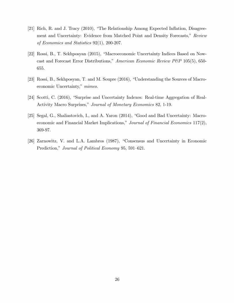
[21] Rich, R. and J. Tracy (2010), �The Relationship Among Expected In�ation, Disagree-

ment and Uncertainty: Evidence from Matched Point and Density Forecasts,�Review

of Economics and Statistics 92(1), 200-207.

[22] Rossi, B., T. Sekhposyan (2015), �Macroeconomic Uncertainty Indices Based on Now-

cast and Forecast Error Distributions,�American Economic Review P&P 105(5), 650-

655.

[23] Rossi, B., Sekhposyan, T. and M. Soupre (2016), �Understanding the Sources of Macro-

economic Uncertainty,�mimeo.

[24] Scotti, C. (2016), �Surprise and Uncertainty Indexes: Real-time Aggregation of Real-

Activity Macro Surprises,�Journal of Monetary Economics 82, 1-19.

[25] Segal, G., Shaliastovich, I., and A. Yaron (2014), �Good and Bad Uncertainty: Macro-

economic and Financial Market Implications,�Journal of Financial Economics 117(2),

369-97.

[26] Zarnowitz, V. and L.A. Lambros (1987), �Consensus and Uncertainty in Economic

Prediction,�Journal of Political Economy 95, 591�621.

26

8 Figures and Tables

Figure 1. Empirical Distribution of the ECB-SPF Forecast Errors

Panel A: In�ation Rate

­3 ­2 ­1 0 1 2 30

0.005

0.01

0.015

0.02

0.025

0.03

0.035

0.04

e

f(e)

PDF of One­Year­Ahead Inflation Forecast Errors

2011:III2013:IIDistribution

­3 ­2 ­1 0 1 2 30

0.1

0.2

0.3

0.4

0.5

0.6

0.7

0.8

0.9

1

e

F(e

)

CDF of One­Year­Ahead Inflation Forecast Errors

2011:III2013:IIDistribution

­3 ­2 ­1 0 1 2 30.5

0.55

0.6

0.65

0.7

0.75

0.8

0.85

0.9

0.95

1

e

Unc

erta

inty

 Indi

ces

Index based on One­Year­Ahead Inflation Forecast

Ut+ h­  ­ 2011:III

Ut+ h+  ­ 2013:II

Panel B: Output Growth

­8 ­7 ­6 ­5 ­4 ­3 ­2 ­1 0 1 2 3 40

0.005

0.01

0.015

0.02

0.025

0.03

0.035

0.04

e

f(e)

PDF of One­Year­Ahead Output Growth Forecast Errors

2011:III2013:IIDistribution

­8 ­7 ­6 ­5 ­4 ­3 ­2 ­1 0 1 2 3 40

0.1

0.2

0.3

0.4

0.5

0.6

0.7

0.8

0.9

1

e

F(e

)

CDF of One­Year­Ahead Output Growth Forecast Errors

2011:III2013:IIDistribution

­8 ­7 ­6 ­5 ­4 ­3 ­2 ­1 0 1 2 3 40.5

0.55

0.6

0.65

0.7

0.75

0.8

0.85

0.9

0.95

1

e

Unc

erta

inty

 Indi

ces

Index based on One­Year­Ahead Output Growth Forecast

Ut+ h­  ­ 2011:III

Ut+ h+  ­ 2013:II

Panel C: Unemployment Rate

­2 ­1 0 1 2 30

0.005

0.01

0.015

0.02

0.025

0.03

e

f(e)

PDF of One­Year­Ahead Unemployment Rate Forecast Errors

2011:III2013:IIDistribution

­2 ­1 0 1 2 30

0.1

0.2

0.3

0.4

0.5

0.6

0.7

0.8

0.9

1

e

F(e

)

CDF of One­Year­Ahead Unemployment Rate Forecast Errors

2011:III2013:IIDistribution

­2 ­1 0 1 2 30.5

0.55

0.6

0.65

0.7

0.75

0.8

0.85

0.9

0.95

1

e

Unc

erta

inty

 Indi

ces

Index based on One­Year­Ahead Unemployment Rate Forecast

Ut+ h­  ­ 2011:III

Ut+ h+  ­ 2013:II

Note: The �gures dep ict the empirica l PDFs and CDFs of forecast errors of H ICP in�ation rate (Panel A ), rea l GDP growth (Panel B ) and

unemployment rate (Panel C ) in the ECB-SPF, together w ith two realizations of forecast errors. The �rst rea lization , 2011:I I I, corresp onds to the

p eak of the latest business cycle, while the second realization , 2013:I I, is one-quarter after its trough . The forecast error realizations are computed

based on �nal release values.

27

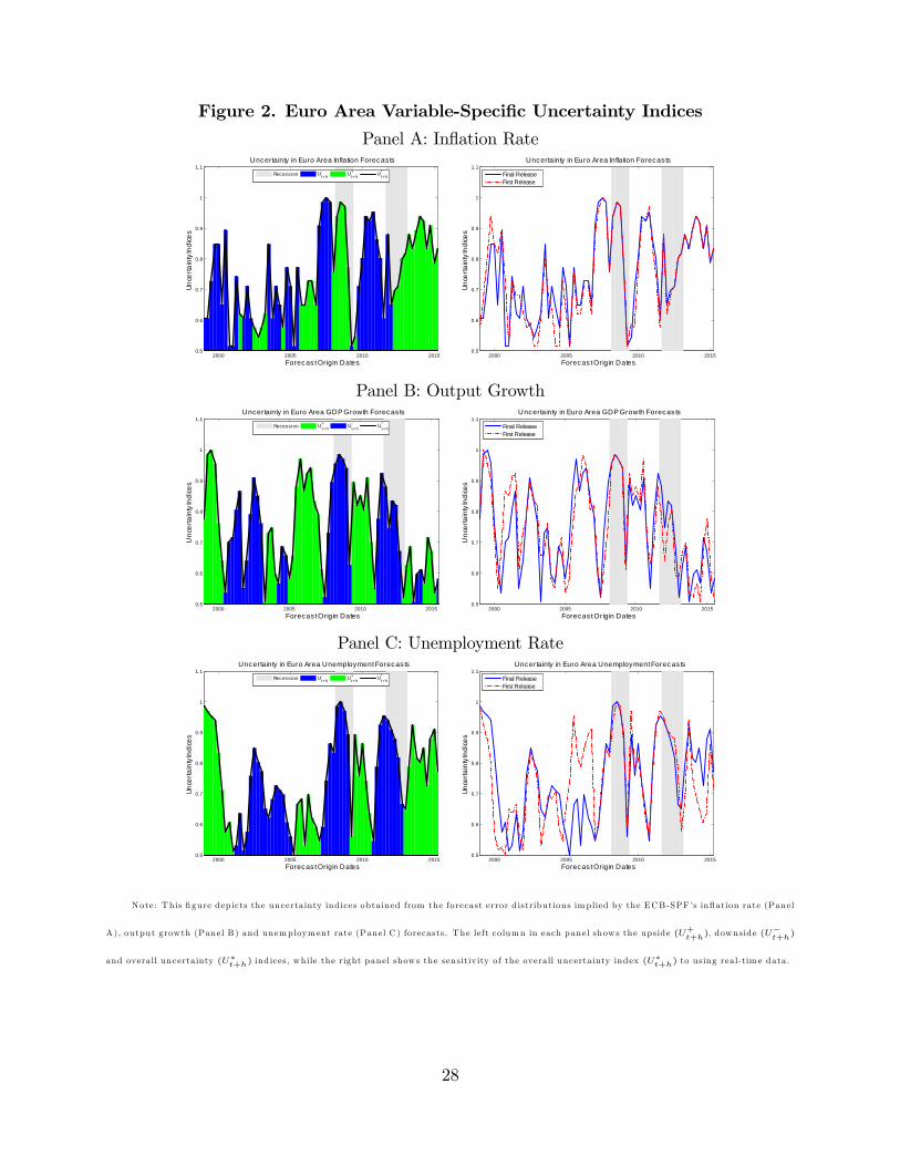
Figure 2. Euro Area Variable-Speci�c Uncertainty Indices

Panel A: In�ation Rate

2000 2005 2010 20150.5

0.6

0.7

0.8

0.9

1

1.1

Forecas t Origin Dates

Unce

rtain

ty In

dice

s

Uncertainty  in Euro Area Inflation Forecasts

Recession Ut+ h­ Ut+ h

+ Ut+ h*

2000 2005 2010 20150.5

0.6

0.7

0.8

0.9

1

1.1

Forecas t Origin Dates

Unce

rtain

ty In

dice

s

Uncertainty  in Euro Area Inflation Forecasts

Final ReleaseFirst Release

Panel B: Output Growth

2000 2005 2010 20150.5

0.6

0.7

0.8

0.9

1

1.1

Forecast Origin Dates

Unc

erta

inty 

Indi

ces

Uncertainty  in Euro Area GDP Growth Forecas ts

Recession Ut+h+ Ut+h

­ Ut+h*

2000 2005 2010 20150.5

0.6

0.7

0.8

0.9

1

1.1

Forecast Origin Dates

Unc

erta

inty 

Indi

ces

Uncertainty  in Euro Area GDP Growth Forecas ts

Final ReleaseFirst Release

Panel C: Unemployment Rate

2000 2005 2010 20150.5

0.6

0.7

0.8

0.9

1

1.1

Forecas t Origin Dates

Unce

rtain

ty In

dice

s

Uncertainty  in Euro Area Unemployment Forecasts

Recession Ut+ h­ Ut+ h

+ Ut+ h*

2000 2005 2010 20150.5

0.6

0.7

0.8

0.9

1

1.1

Forecas t Origin Dates

Unce

rtain

ty In

dice

s

Uncertainty  in Euro Area Unemployment Forecasts

Final ReleaseFirst Release

Note: This �gure dep icts the uncerta inty ind ices obtained from the forecast error d istributions implied by the ECB-SPF�s in�ation rate (Panel

A ), output grow th (Panel B ) and unemploym ent rate (Panel C ) forecasts. The left co lumn in each panel shows the upside (U+t+h

), downside (U�t+h

)

and overall uncerta inty (U�t+h) ind ices, while the right panel shows the sensitiv ity of the overall uncerta inty index (U�t+h) to using real-tim e data.

28

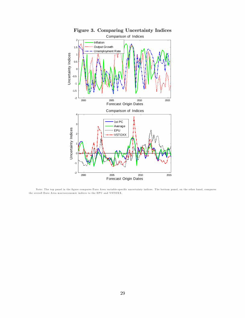
Figure 3. Comparing Uncertainty Indices

2000 2005 2010 2015­2

­1.5

­1

­0.5

0

0.5

1

1.5

2

Forecast Origin Dates

Unc

erta

inty

 Indi

ces

Comparison of  IndicesInflationOutput GrowthUnemployment Rate

2000 2005 2010 2015­2

­1

0

1

2

3

4

Forecast Origin Dates

Unc

erta

inty

 Indi

ces

Comparison of  Indices

1st PCAverageEPUVSTOXX

Note: The top panel in the �gure compares Euro Area variab le-sp eci�c uncerta inty ind ices. The bottom panel, on the other hand, compares

the overall Euro Area macro econom ic ind ices to the EPU and VSTOXX.

29

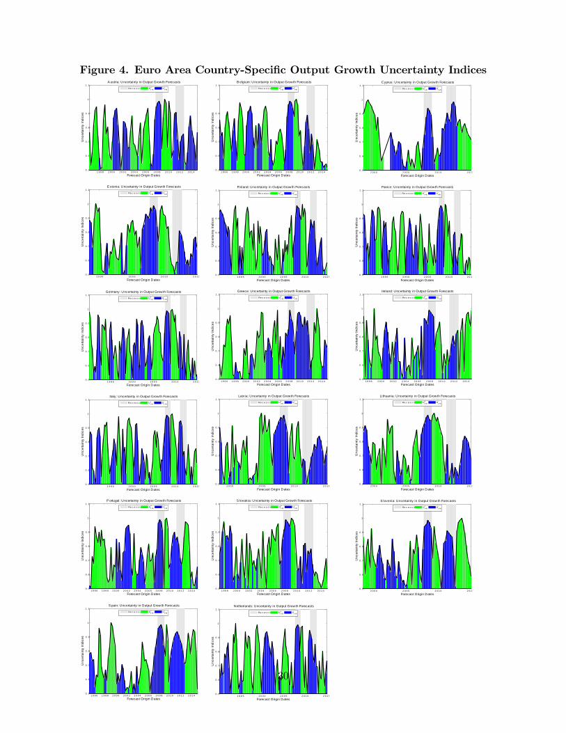
Figure 4. Euro Area Country-Speci�c Output Growth Uncertainty Indices

1 9 9 8 2 0 0 0 2 0 0 2 2 0 0 4 2 0 0 6 2 0 0 8 2 0 1 0 2 0 1 2 2 0 1 40 . 5

0 . 6

0 . 7

0 . 8

0 . 9

1

1 . 1

Forecast Origin Dates

Unc

erta

inty

 Indi

ces

A ustria: Uncertainty in Output Grow th Forecasts

Re c e s s i o n Ut +h+ Ut +h

­

1 9 9 6 1 9 9 8 2 0 0 0 2 0 0 2 2 0 0 4 2 0 0 6 2 0 0 8 2 0 1 0 2 0 1 2 2 0 1 40 . 5

0 . 6

0 . 7

0 . 8

0 . 9

1

1 . 1

Forecast Origin Dates

Unc

erta

inty

 Indi

ces

B elgium: Uncertainty in Output Growth Forecasts

Re c e s s i o n Ut +h+ Ut +h

­

2 0 0 0 2 0 0 5 2 0 1 0 2 0 1 50 .5

0 .6

0 .7

0 .8

0 .9

1

1 .1

Forecast Origin Dates

Unc

erta

inty

 Indi

ces

C yprus: Uncertainty in Output Growth Forecasts

Re c e s s i o n Ut +h+ Ut +h

­

2 0 0 0 2 0 0 5 2 0 1 0 2 0 1 50 .5

0 .6

0 .7

0 .8

0 .9

1

1 .1

Forecast Origin Dates

Unc

erta

inty

 Indi

ces

E stonia: U ncertainty in Output Growth Forecasts

Re c e s s i o n Ut +h+ Ut +h

­

1 9 9 5 2 0 0 0 2 0 0 5 2 0 1 0 2 0 1 50 .5

0 .6

0 .7

0 .8

0 .9

1

1 .1

Forecast Origin Dates

Unc

erta

inty

 Indi

ces

Finland: Uncertainty in Output Growth Forecasts

Re c e s s i o n Ut +h+ Ut +h

­

1 9 9 5 2 0 0 0 2 0 0 5 2 0 1 0 2 0 1 50 .5

0 .6

0 .7

0 .8

0 .9

1

1 .1

Forecast Origin Dates

Unc

erta

inty

 Indi

ces

France: Uncertainty in Output Growth Forecasts

Re c e s s i o n Ut +h+ Ut +h

­

1 9 9 5 2 0 0 0 2 0 0 5 2 0 1 0 2 0 1 50 .5

0 .6

0 .7

0 .8

0 .9

1

1 .1

Forecast Origin Dates

Unc

erta

inty

 Indi

ces

Germany: Uncertainty in Output Growth Forecasts

Re c e s s i o n Ut +h+ Ut +h

­

1 9 9 6 1 9 9 8 2 0 0 0 2 0 0 2 2 0 0 4 2 0 0 6 2 0 0 8 2 0 1 0 2 0 1 2 2 0 1 40 . 5

0 . 6

0 . 7

0 . 8

0 . 9

1

1 . 1

Forecast Origin Dates

Unc

erta

inty

 Indi

ces

Greece: Uncertainty in Output Growth Forecasts

Re c e s s i o n Ut +h+ Ut +h

­

1 9 9 8 2 0 0 0 2 0 0 2 2 0 0 4 2 0 0 6 2 0 0 8 2 0 1 0 2 0 1 2 2 0 1 40 . 5

0 . 6

0 . 7

0 . 8

0 . 9

1

1 . 1

Forecast Origin Dates

Unc

erta

inty

 Indi

ces

Ireland: Uncertainty in Output Growth Forecasts

Re c e s s i o n Ut +h+ Ut +h

­

1 9 9 5 2 0 0 0 2 0 0 5 2 0 1 0 2 0 1 50 .5

0 .6

0 .7

0 .8

0 .9

1

1 .1

Forecast Origin Dates

Unc

erta

inty

 Indi

ces

Italy: Uncertainty in Output Growth Forecasts

Re c e s s i o n Ut +h+ Ut +h

­

2 0 0 0 2 0 0 5 2 0 1 0 2 0 1 50 .5

0 .6

0 .7

0 .8

0 .9

1

1 .1

Forecast Origin Dates

Unc

erta

inty

 Indi

ces

Latvia: Uncertainty in Output Grow th Forecasts

Re c e s s i o n Ut +h+ Ut +h

­

2 0 0 0 2 0 0 5 2 0 1 0 2 0 1 50 .5

0 .6

0 .7

0 .8

0 .9

1

1 .1

Forecast Origin Dates

Unc

erta

inty

 Indi

ces

Lithuania: Uncertainty in Output Grow th Forecasts

Re c e s s i o n Ut +h+ Ut +h

­

1 9 9 6 1 9 9 8 2 0 0 0 2 0 0 2 2 0 0 4 2 0 0 6 2 0 0 8 2 0 1 0 2 0 1 2 2 0 1 40 . 5

0 . 6

0 . 7

0 . 8

0 . 9

1

1 . 1

Forecast Origin Dates

Unc

erta

inty

 Indi

ces

P ortugal: Uncertainty in Output Growth Forecasts

Re c e s s i o n Ut +h+ Ut +h

­

1 9 9 8 2 0 0 0 2 0 0 2 2 0 0 4 2 0 0 6 2 0 0 8 2 0 1 0 2 0 1 2 2 0 1 40 . 5

0 . 6

0 . 7

0 . 8

0 . 9

1

1 . 1

Forecast Origin Dates

Unc

erta

inty

 Indi

ces

S lovakia: U ncertainty in Output Growth Forecasts

Re c e s s i o n Ut +h+ Ut +h

­

2 0 0 0 2 0 0 5 2 0 1 0 2 0 1 50 .5

0 .6

0 .7

0 .8

0 .9

1

1 .1

Forecast Origin Dates

Unc

erta

inty

 Indi

ces

S lovenia: Uncertainty in Output Grow th Forecasts

Re c e s s i o n Ut +h+ Ut +h

­

1 9 9 6 1 9 9 8 2 0 0 0 2 0 0 2 2 0 0 4 2 0 0 6 2 0 0 8 2 0 1 0 2 0 1 2 2 0 1 40 . 5

0 . 6

0 . 7

0 . 8

0 . 9

1

1 . 1

Forecast Origin Dates

Unc

erta

inty

 Indi

ces

S pain: Uncertainty in Output Growth Forecasts

Re c e s s i o n Ut +h+ Ut +h

­

1 9 9 5 2 0 0 0 2 0 0 5 2 0 1 0 2 0 1 50 .5

0 .6

0 .7

0 .8

0 .9

1

1 .1

Forecast Origin Dates

Unc

erta

inty

 Indi

ces

Netherlands: Uncertainty in Output Growth Forecasts

Re c e s s i o n Ut +h+ Ut +h

­

30

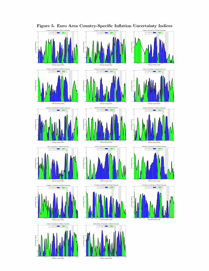
Figure 5. Euro Area Country-Speci�c In�ation Uncertainty Indices

1 9 9 5 2 0 0 0 2 0 0 5 2 0 1 0 2 0 1 50 .5

0 .6

0 .7

0 .8

0 .9

1

1 .1

Forecast Origin Dates

Unc

erta

inty

 Indi

ces

A ustria: Uncertainty in Inflation Forecasts

Re c e s s i o n Ut +h­ Ut +h

+

1 9 9 5 2 0 0 0 2 0 0 5 2 0 1 0 2 0 1 50 .5

0 .6

0 .7

0 .8

0 .9

1

1 .1

Forecast Origin Dates

Unc

erta

inty

 Indi

ces

B elgium: Uncertainty in Inflation Forecasts

Re c e s s i o n Ut +h­ Ut +h

+

2 0 0 0 2 0 0 5 2 0 1 0 2 0 1 50 .5

0 .6

0 .7

0 .8

0 .9

1

1 .1

Forecast Origin Dates

Unc

erta

inty

 Indi

ces

C yprus: Uncertainty in Inflation Forecasts

Re c e s s i o n Ut +h­ Ut +h

+

2 0 0 0 2 0 0 5 2 0 1 0 2 0 1 50 .5

0 .6

0 .7

0 .8

0 .9

1

1 .1

Forecast Origin Dates

Unc

erta

inty

 Indi

ces

E stonia: U ncertainty in Inflation Forecasts

Re c e s s i o n Ut +h­ Ut +h

+

1 9 9 5 2 0 0 0 2 0 0 5 2 0 1 0 2 0 1 50 .5

0 .6

0 .7

0 .8

0 .9

1

1 .1

Forecast Origin Dates

Unc

erta

inty

 Indi

ces

Finland: Uncertainty in Inflation Forecasts

Re c e s s i o n Ut +h­ Ut +h

+

1 9 9 5 2 0 0 0 2 0 0 5 2 0 1 0 2 0 1 50 .5

0 .6

0 .7

0 .8

0 .9

1

1 .1

Forecast Origin Dates

Unc

erta

inty

 Indi

ces

France: Uncertainty in Inflation Forecasts

Re c e s s i o n Ut +h­ Ut +h

+

1 9 9 5 2 0 0 0 2 0 0 5 2 0 1 0 2 0 1 50 .5

0 .6

0 .7

0 .8

0 .9

1

1 .1

Forecast Origin Dates

Unc

erta

inty

 Indi

ces

Germany: Uncertainty in Inflation Forecasts

Re c e s s i o n Ut +h­ Ut +h

+

1 9 9 4 1 9 9 6 1 9 9 8 2 0 0 0 2 0 0 2 2 0 0 4 2 0 0 6 2 0 0 8 2 0 1 0 2 0 1 2 2 0 1 40 . 5

0 . 6

0 . 7

0 . 8

0 . 9

1

1 . 1

Forecast Origin Dates

Unc

erta

inty

 Indi

ces

Greece: Uncertainty in Inflation Forecasts

Re c e s s i o n Ut +h­ Ut +h

+

1 9 9 5 2 0 0 0 2 0 0 5 2 0 1 0 2 0 1 50 .5

0 .6

0 .7

0 .8

0 .9

1

1 .1

Forecast Origin Dates

Unc

erta

inty

 Indi

ces

Ireland: Uncertainty in Inflation Forecasts

Re c e s s i o n Ut +h­ Ut +h

+

1 9 9 5 2 0 0 0 2 0 0 5 2 0 1 0 2 0 1 50 .5

0 .6

0 .7

0 .8

0 .9

1

1 .1

Forecast Origin Dates

Unc

erta

inty

 Indi

ces

Italy: Uncertainty in Inflation Forecasts

Re c e s s i o n Ut +h­ Ut +h

+

2 0 0 0 2 0 0 5 2 0 1 0 2 0 1 50 .5

0 .6

0 .7

0 .8

0 .9

1

1 .1

Forecast Origin Dates

Unc

erta

inty

 Indi

ces

Latvia: Uncertainty in Inflation Forecasts

Re c e s s i o n Ut +h­ Ut +h

+

2 0 0 0 2 0 0 5 2 0 1 0 2 0 1 50 .5

0 .6

0 .7

0 .8

0 .9

1

1 .1

Forecast Origin Dates

Unc

erta

inty

 Indi

ces

Lithuania: Uncertainty in Inflation Forecasts

Re c e s s i o n Ut +h­ Ut +h

+

1 9 9 5 2 0 0 0 2 0 0 5 2 0 1 0 2 0 1 50 .5

0 .6

0 .7

0 .8

0 .9

1

1 .1

Forecast Origin Dates

Unc

erta

inty

 Indi

ces

P ortugal: Uncertainty in Inflation Forecasts

Re c e s s i o n Ut +h­ Ut +h

+

1 9 9 6 1 9 9 8 2 0 0 0 2 0 0 2 2 0 0 4 2 0 0 6 2 0 0 8 2 0 1 0 2 0 1 2 2 0 1 40 . 5

0 . 6

0 . 7

0 . 8

0 . 9

1

1 . 1

Forecast Origin Dates

Unc

erta

inty

 Indi

ces

S lovakia: U ncertainty in Inflation Forecasts

Re c e s s i o n Ut +h­ Ut +h

+

1 9 9 6 1 9 9 8 2 0 0 0 2 0 0 2 2 0 0 4 2 0 0 6 2 0 0 8 2 0 1 0 2 0 1 2 2 0 1 40 . 5

0 . 6

0 . 7

0 . 8

0 . 9

1

1 . 1

Forecast Origin Dates

Unc

erta

inty

 Indi

ces

S lovenia: U ncertainty in Inflation Forecasts

Re c e s s i o n Ut +h­ Ut +h

+

1 9 9 5 2 0 0 0 2 0 0 5 2 0 1 0 2 0 1 50 .5

0 .6

0 .7

0 .8

0 .9

1

1 .1

Forecast Origin Dates

Unc

erta

inty

 Indi

ces

S pain: Uncertainty in Inflation Forecasts

Re c e s s i o n Ut +h­ Ut +h

+

1 9 9 5 2 0 0 0 2 0 0 5 2 0 1 0 2 0 1 50 .5

0 .6

0 .7

0 .8

0 .9

1

1 .1

Forecast Origin Dates

Unc

erta

inty

 Indi

ces

Netherlands: Uncertainty in Inflation Forecasts

Re c e s s i o n Ut +h­ Ut +h

+

31

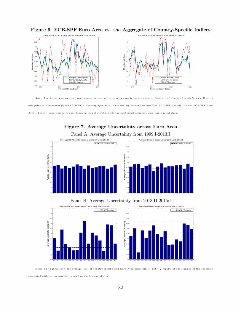
Figure 6. ECB-SPF Euro Area vs. the Aggregate of Country-Speci�c Indices

2000 2005 2010 20150.5

0.55

0.6

0.65

0.7

0.75

0.8

0.85

0.9

0.95

1

Forec as t Origin Dates

Unce

rtain

ty In

dice

s

Comparison of Unc ertainty  Indices  Based on GDP Growth

Average of Country­Specific1st PC of Country­SpecificECB­SPF Euro Area

2000 2005 2010 20150.5

0.55

0.6

0.65

0.7

0.75

0.8

0.85

0.9

0.95

1

Forecas t Origin Dates

Unce

rtain

ty In

dice

s

Comparison of Uncertainty  Indices  Based on Inflation

Average of Country­Specific1st PC of Country­SpecificECB­SPF Euro Area

Note: The �gure compares the cross-country average of the country-sp eci�c ind ices (lab eled "Average of Country-Sp eci�c"), as well as its

�rst principal component (lab eled "1st PC of Country-Sp eci�c"), to uncerta inty ind ices obtained from ECB-SPF directly (lab eled ECB-SPF Euro

Area). The left panel compares uncerta inty in output grow th , while the right panel compares uncerta inty in in�ation .

Figure 7. Average Uncertainty across Euro Area

Panel A: Average Uncertainty from 1999:I-2013:I

AUT BEL CYP EST FIN FRA DEU GRC IRL ITA L VA L TU PRT SVK SVN ESP NL D0 .5

0 .5 5

0 .6

0 .6 5

0 .7

0 .7 5

0 .8

0 .8 5

0 .9

0 .9 5

1

Aver

age 

Leve

l of U

ncer

tain

ty

Average GDP Growth­based Uncertainty Up to 2013:II

ECB­SPF Euro Area

AUT BEL CYP EST FIN FRA DEU GRC IRL ITA L VA L TU PRT SVK SVN ESP NL D0 .5

0 .5 5

0 .6

0 .6 5

0 .7

0 .7 5

0 .8

0 .8 5

0 .9

0 .9 5

1

Aver

age 

Leve

l of U

ncer

tain

ty

Average Inflation­based Uncertainty Up to 2013:II

ECB­SPF Euro Area

Panel B: Average Uncertainty from 2013:II-2015:I

AUT BEL CYP EST FIN FRA DEU GRC IRL ITA L VA L TU PRT SVK SVN ESP NL D0 .5

0 .5 5

0 .6

0 .6 5

0 .7

0 .7 5

0 .8

0 .8 5

0 .9

0 .9 5

1

Aver

age 

Leve

l of U

ncer

tain

ty

Average GDP Growth­based Uncertainty Since 2013:II

ECB­SPF Euro Area

AUT BEL CYP EST FIN FRA DEU GRC IRL ITA L VA L TU PRT SVK SVN ESP NL D0 .5

0 .5 5

0 .6

0 .6 5

0 .7

0 .7 5

0 .8

0 .8 5

0 .9

0 .9 5

1

Aver

age 

Leve

l of U

ncer

tain

ty

Average Inflation­based Uncertainty s ince 2013:II

ECB­SPF Euro Area

Note: The �gures show the average level o f country-sp eci�c and Euro Area uncerta inty. Table 2 rep orts the fu ll nam es of the countries

asso ciated w ith the mnemonics rep orted on the horizontal ax is.

32

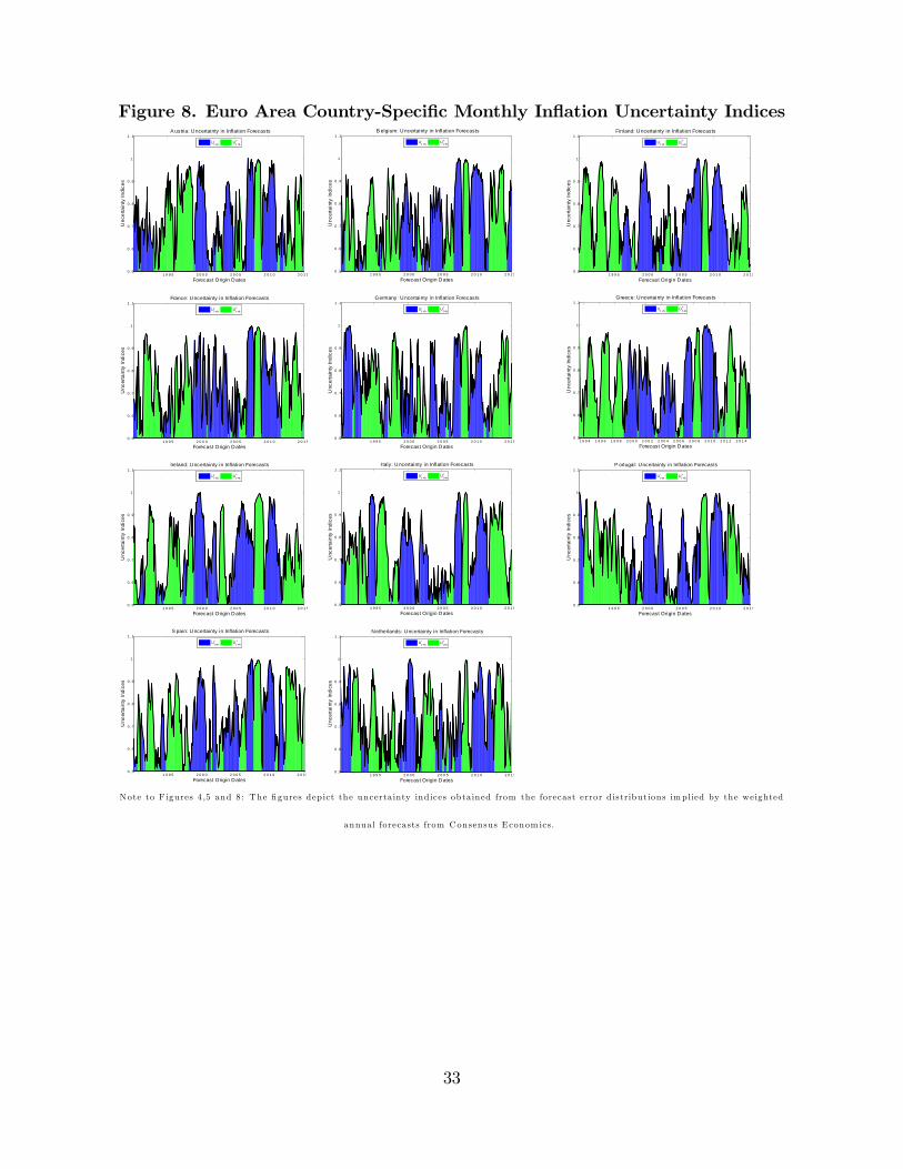
Figure 8. Euro Area Country-Speci�c Monthly In�ation Uncertainty Indices

1 9 9 5 2 0 0 0 2 0 0 5 2 0 1 0 2 0 1 50 .5

0 .6

0 .7

0 .8

0 .9

1

1 .1

Forecast Origin D ates

Unc

erta

inty

 Indi

ces

A ustria: Uncertainty in Inflation Forecasts

Ut +h­ Ut +h

+

1 9 9 5 2 0 0 0 2 0 0 5 2 0 1 0 2 0 1 50 .5

0 .6

0 .7

0 .8

0 .9

1

1 .1

Forecast Origin D ates

Unc

erta

inty

 Indi

ces

B elgium: Uncertainty in Inflation Forecasts

Ut +h­ Ut +h

+

1 9 9 5 2 0 0 0 2 0 0 5 2 0 1 0 2 0 1 50 .5

0 .6

0 .7

0 .8

0 .9

1

1 .1

Forecast Origin D ates

Unc

erta

inty

 Indi

ces

Finland: Uncertainty in Inflation Forecasts

Ut +h­ Ut +h

+

1 9 9 5 2 0 0 0 2 0 0 5 2 0 1 0 2 0 1 50 .5

0 .6

0 .7

0 .8

0 .9

1

1 .1

Forecast Origin D ates

Unc

erta

inty

 Indi

ces

France: Uncertainty in Inflation Forecasts

Ut +h­ Ut +h

+

1 9 9 5 2 0 0 0 2 0 0 5 2 0 1 0 2 0 1 50 .5

0 .6

0 .7

0 .8

0 .9

1

1 .1

Forecast Origin D ates

Unc

erta

inty

 Indi

ces

Germany: Uncertainty in Inflation Forecasts

Ut +h­ Ut +h

+

1 9 9 4 1 9 9 6 1 9 9 8 2 0 0 0 2 0 0 2 2 0 0 4 2 0 0 6 2 0 0 8 2 0 1 0 2 0 1 2 2 0 1 40 .5

0 .6

0 .7

0 .8

0 .9

1

1 .1

Forecast Origin Dates

Unc

erta

inty

 Indi

ces

Greece: Uncertainty in Inflation Forecasts

Ut +h­ Ut +h

+

1 9 9 5 2 0 0 0 2 0 0 5 2 0 1 0 2 0 1 50 .5

0 .6

0 .7

0 .8

0 .9

1

1 .1

Forecast Origin D ates

Unc

erta

inty

 Indi

ces

Ireland: Uncertainty in Inflation Forecasts

Ut +h­ Ut +h

+

1 9 9 5 2 0 0 0 2 0 0 5 2 0 1 0 2 0 1 50 .5

0 .6

0 .7

0 .8

0 .9

1

1 .1

Forecast Origin D ates

Unc

erta

inty

 Indi

ces

Italy: U ncertainty in Inflation Forecasts

Ut +h­ Ut +h

+

1 9 9 5 2 0 0 0 2 0 0 5 2 0 1 0 2 0 1 50 .5

0 .6

0 .7

0 .8

0 .9

1

1 .1

Forecast Origin D ates

Unc

erta

inty

 Indi

ces

P ortugal: Uncertainty in Inflation Forecasts

Ut +h­ Ut +h

+

1 9 9 5 2 0 0 0 2 0 0 5 2 0 1 0 2 0 1 50 .5

0 .6

0 .7

0 .8

0 .9

1

1 .1

Forecast Origin D ates

Unc

erta

inty

 Indi

ces

S pain: Uncertainty in Inflation Forecasts

Ut +h­ Ut +h

+

1 9 9 5 2 0 0 0 2 0 0 5 2 0 1 0 2 0 1 50 .5

0 .6

0 .7

0 .8

0 .9

1

1 .1

Forecast Origin D ates

Unc

erta

inty

 Indi

ces

Netherlands: Uncertainty in Inflation Forecasts

Ut +h­ Ut +h

+

Note to F igures 4 ,5 and 8: The �gures dep ict the uncerta inty ind ices obtained from the forecast error d istributions implied by the weighted

annual forecasts from Consensus Econom ics.

33

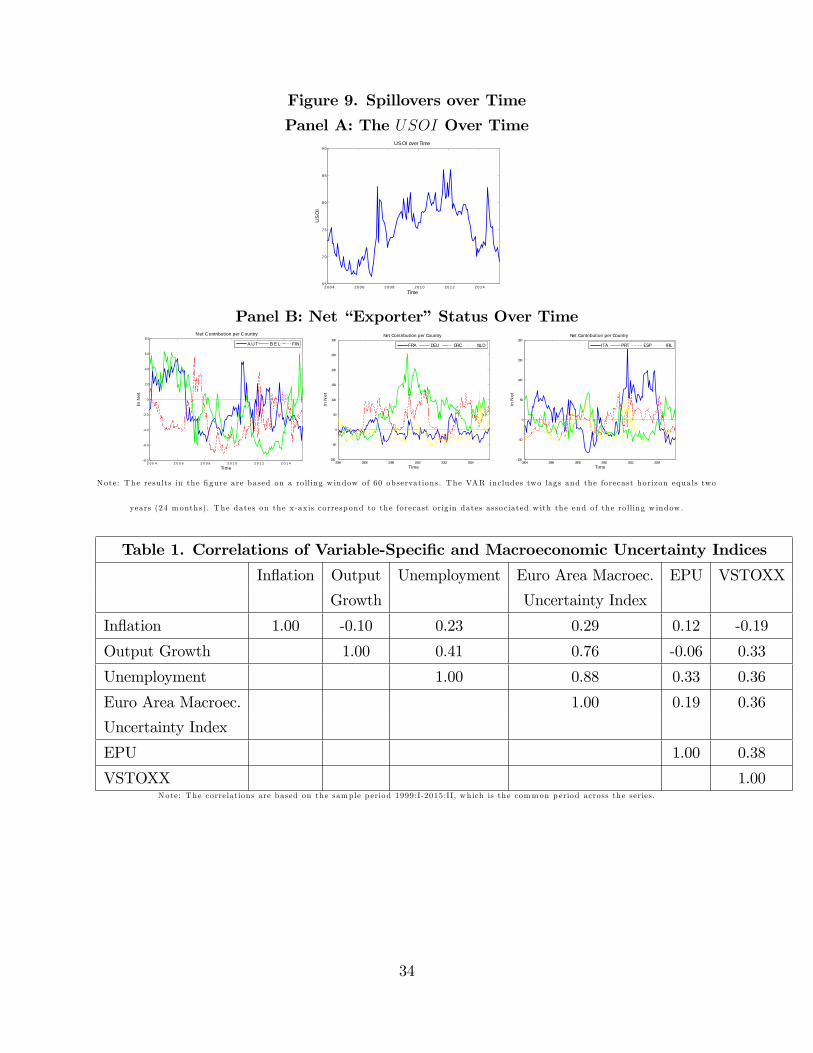
Figure 9. Spillovers over Time

Panel A: The USOI Over Time

2 0 0 4 2 0 0 6 2 0 0 8 2 0 1 0 2 0 1 2 2 0 1 46 5

7 0

7 5

8 0

8 5

9 0USOI over Time

Time

US

OI

Panel B: Net �Exporter�Status Over Time

2 0 0 4 2 0 0 6 2 0 0 8 2 0 1 0 2 0 1 2 2 0 1 4­8 0

­6 0

­4 0

­2 0

0

2 0

4 0

6 0

8 0Net C ontribution per Country

Time

In N

et

A U T B E L FIN

2004 2006 2008 2010 2012 2014­100

­50

0

50

100

150

200

250

300Net Contribution per Country

Time

In N

et

FRA DEU GRC NLD

2004 2006 2008 2010 2012 2014­100

­50

0

50

100

150

200Net Contribution per Country

Time

In N

et

ITA PRT ESP IRL

Note: The resu lts in the �gure are based on a rolling w indow of 60 observations. The VAR includes two lags and the forecast horizon equals two

years (24 months). The dates on the x-axis corresp ond to the forecast orig in dates asso ciated w ith the end of the rolling w indow .

Table 1. Correlations of Variable-Speci�c and Macroeconomic Uncertainty Indices

In�ation Output Unemployment Euro Area Macroec. EPU VSTOXX

Growth Uncertainty Index

In�ation 1.00 -0.10 0.23 0.29 0.12 -0.19

Output Growth 1.00 0.41 0.76 -0.06 0.33

Unemployment 1.00 0.88 0.33 0.36

Euro Area Macroec. 1.00 0.19 0.36

Uncertainty Index

EPU 1.00 0.38

VSTOXX 1.00Note: The correlations are based on the sample p eriod 1999:I-2015:I I, which is the common p eriod across the series.

34

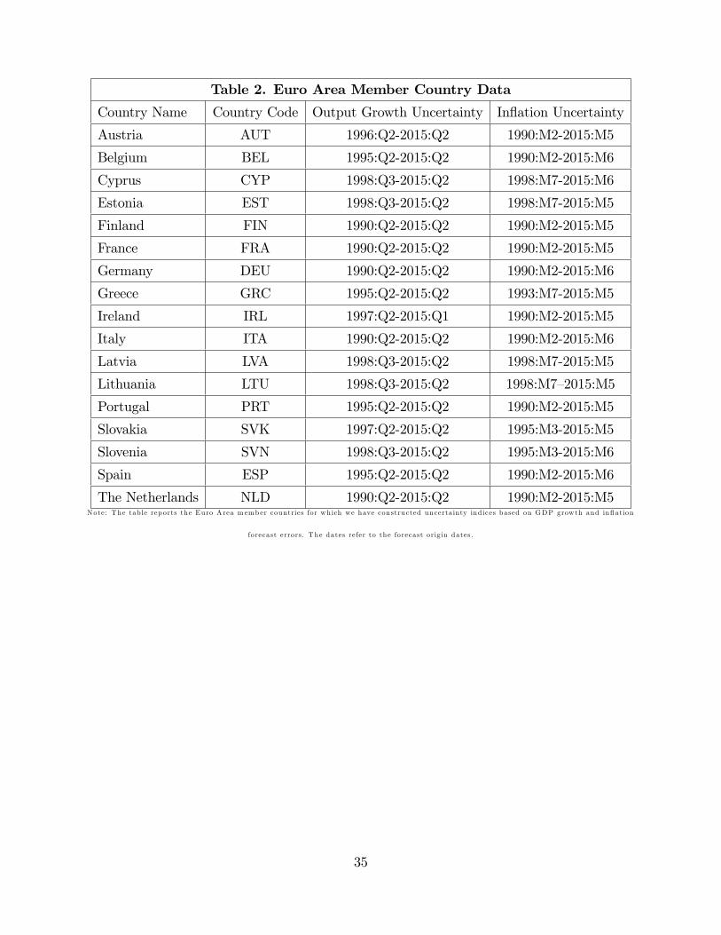
Table 2. Euro Area Member Country Data

Country Name Country Code Output Growth Uncertainty In�ation Uncertainty

Austria AUT 1996:Q2-2015:Q2 1990:M2-2015:M5

Belgium BEL 1995:Q2-2015:Q2 1990:M2-2015:M6

Cyprus CYP 1998:Q3-2015:Q2 1998:M7-2015:M6

Estonia EST 1998:Q3-2015:Q2 1998:M7-2015:M5

Finland FIN 1990:Q2-2015:Q2 1990:M2-2015:M5

France FRA 1990:Q2-2015:Q2 1990:M2-2015:M5

Germany DEU 1990:Q2-2015:Q2 1990:M2-2015:M6

Greece GRC 1995:Q2-2015:Q2 1993:M7-2015:M5

Ireland IRL 1997:Q2-2015:Q1 1990:M2-2015:M5

Italy ITA 1990:Q2-2015:Q2 1990:M2-2015:M6

Latvia LVA 1998:Q3-2015:Q2 1998:M7-2015:M5

Lithuania LTU 1998:Q3-2015:Q2 1998:M7�2015:M5

Portugal PRT 1995:Q2-2015:Q2 1990:M2-2015:M5

Slovakia SVK 1997:Q2-2015:Q2 1995:M3-2015:M5

Slovenia SVN 1998:Q3-2015:Q2 1995:M3-2015:M6

Spain ESP 1995:Q2-2015:Q2 1990:M2-2015:M6

The Netherlands NLD 1990:Q2-2015:Q2 1990:M2-2015:M5Note: The tab le rep orts the Euro Area m ember countries for which we have constructed uncerta inty ind ices based on GDP growth and in�ation

forecast errors. The dates refer to the forecast orig in dates.

35

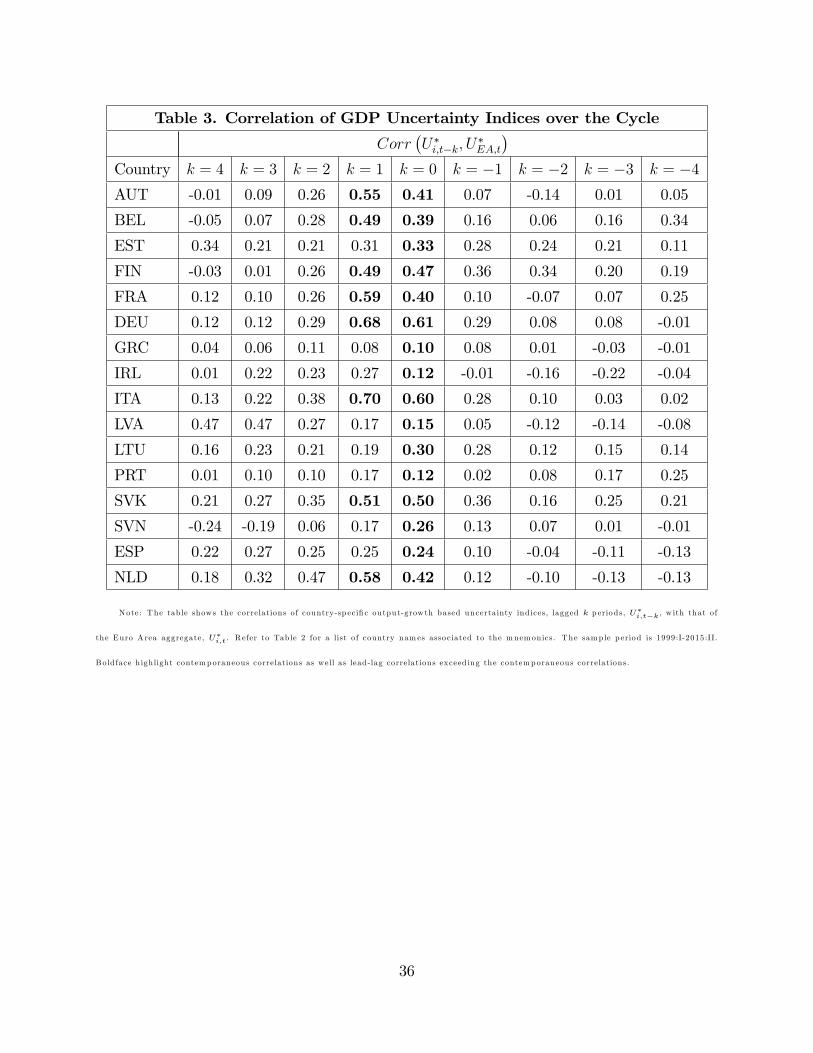
Table 3. Correlation of GDP Uncertainty Indices over the Cycle

Corr�U�i;t�k; U

�EA;t

�Country k = 4 k = 3 k = 2 k = 1 k = 0 k = �1 k = �2 k = �3 k = �4AUT -0.01 0.09 0.26 0.55 0.41 0.07 -0.14 0.01 0.05

BEL -0.05 0.07 0.28 0.49 0.39 0.16 0.06 0.16 0.34

EST 0.34 0.21 0.21 0.31 0.33 0.28 0.24 0.21 0.11

FIN -0.03 0.01 0.26 0.49 0.47 0.36 0.34 0.20 0.19

FRA 0.12 0.10 0.26 0.59 0.40 0.10 -0.07 0.07 0.25

DEU 0.12 0.12 0.29 0.68 0.61 0.29 0.08 0.08 -0.01

GRC 0.04 0.06 0.11 0.08 0.10 0.08 0.01 -0.03 -0.01

IRL 0.01 0.22 0.23 0.27 0.12 -0.01 -0.16 -0.22 -0.04

ITA 0.13 0.22 0.38 0.70 0.60 0.28 0.10 0.03 0.02

LVA 0.47 0.47 0.27 0.17 0.15 0.05 -0.12 -0.14 -0.08

LTU 0.16 0.23 0.21 0.19 0.30 0.28 0.12 0.15 0.14

PRT 0.01 0.10 0.10 0.17 0.12 0.02 0.08 0.17 0.25

SVK 0.21 0.27 0.35 0.51 0.50 0.36 0.16 0.25 0.21

SVN -0.24 -0.19 0.06 0.17 0.26 0.13 0.07 0.01 -0.01

ESP 0.22 0.27 0.25 0.25 0.24 0.10 -0.04 -0.11 -0.13

NLD 0.18 0.32 0.47 0.58 0.42 0.12 -0.10 -0.13 -0.13

Note: The tab le shows the correlations of country-sp eci�c output-grow th based uncerta inty ind ices, lagged k p eriods, U�i;t�k , w ith that of

the Euro Area aggregate, U�i;t. R efer to Table 2 for a list of country names asso ciated to the mnemonics. The sample p eriod is 1999:I-2015:I I.

Bold face h igh light contemporaneous correlations as well as lead-lag correlations exceed ing the contemporaneous correlations.

36

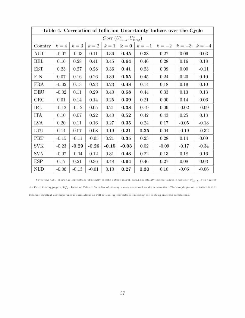
Table 4. Correlation of In�ation Uncertainty Indices over the Cycle

Corr�U�i;t�k; U

�EA;t

�Country k = 4 k = 3 k = 2 k = 1 k = 0 k = �1 k = �2 k = �3 k = �4AUT -0.07 -0.03 0.11 0.36 0.45 0.38 0.27 0.09 0.03

BEL 0.16 0.28 0.41 0.45 0.64 0.46 0.28 0.16 0.18

EST 0.23 0.27 0.28 0.36 0.41 0.23 0.09 0.00 -0.11

FIN 0.07 0.16 0.26 0.39 0.55 0.45 0.24 0.20 0.10

FRA -0.02 0.13 0.23 0.23 0.48 0.14 0.18 0.19 0.10

DEU -0.02 0.11 0.29 0.40 0.58 0.44 0.33 0.13 0.13

GRC 0.01 0.14 0.14 0.25 0.39 0.21 0.00 0.14 0.06

IRL -0.12 -0.12 0.05 0.21 0.38 0.19 0.09 -0.02 -0.09

ITA 0.10 0.07 0.22 0.40 0.52 0.42 0.43 0.25 0.13

LVA 0.20 0.11 0.16 0.27 0.35 0.24 0.17 -0.05 -0.18

LTU 0.14 0.07 0.08 0.19 0.21 0.25 0.04 -0.19 -0.32

PRT -0.15 -0.11 -0.05 0.21 0.35 0.23 0.28 0.14 0.09

SVK -0.23 -0.29 -0.26 -0.15 -0.03 0.02 -0.09 -0.17 -0.34

SVN -0.07 -0.04 0.12 0.31 0.43 0.22 0.13 0.18 0.16

ESP 0.17 0.21 0.36 0.48 0.64 0.46 0.27 0.08 0.03

NLD -0.06 -0.13 -0.01 0.10 0.27 0.30 0.10 -0.06 -0.06

Note: The tab le shows the correlations of country-sp eci�c output-grow th based uncerta inty ind ices, lagged k p eriods, U�i;t�k , w ith that of

the Euro Area aggregate, U�i;t. R efer to Table 2 for a list of country names asso ciated to the mnemonics. The sample p eriod is 1999:I-2015:I.

Bold face h igh light contemporaneous correlations as well as lead-lag correlations exceed ing the contemporaneous correlations.

37

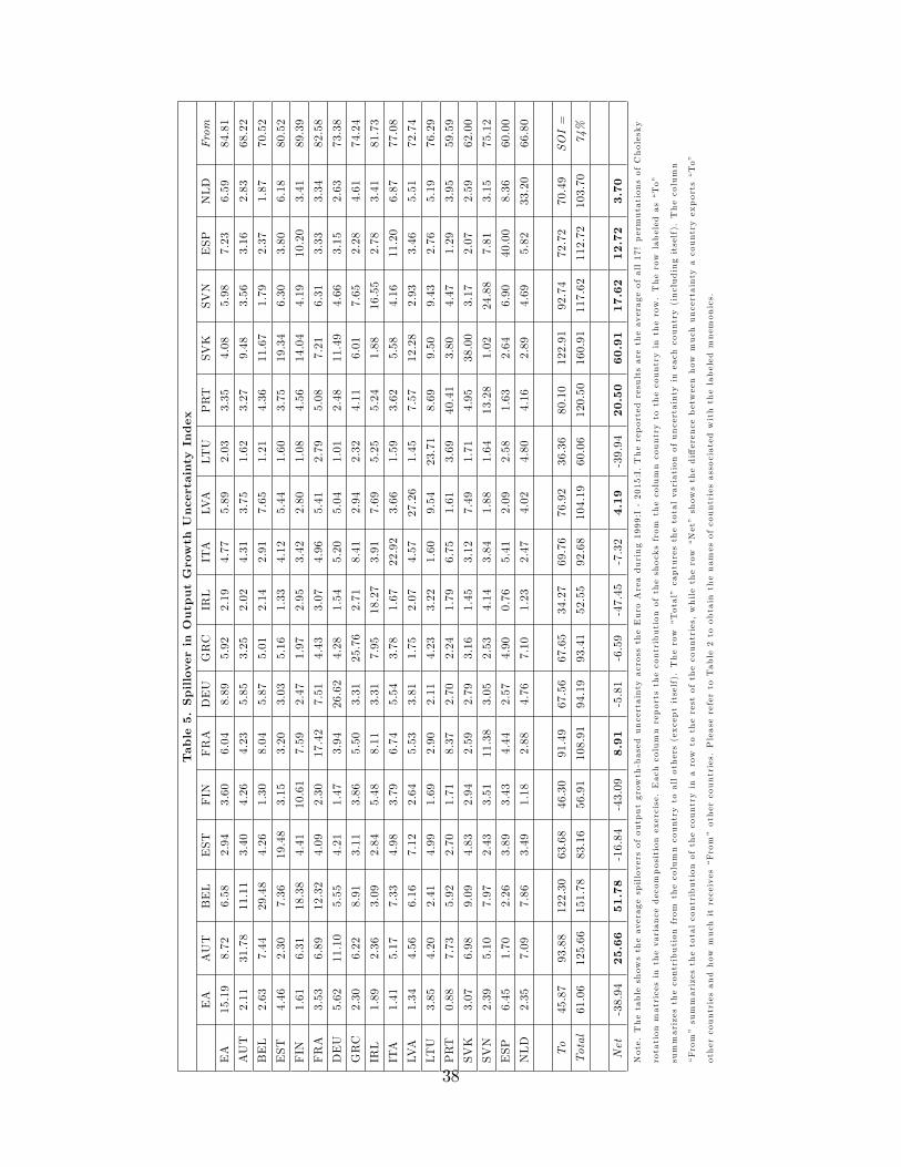
Table5.SpilloverinOutputGrowth

UncertaintyIndex

EA

AUT

BEL

EST

FIN

FRA

DEU

GRC

IRL

ITA

LVA

LTU

PRT

SVK

SVN

ESP

NLD

From

EA

15.19

8.72

6.58

2.94

3.60

6.04

8.89

5.92

2.19

4.77

5.89

2.03

3.35

4.08

5.98

7.23

6.59

84.81

AUT

2.11

31.78

11.11

3.40

4.26

4.23

5.85

3.25

2.02

4.31

3.75

1.62

3.27

9.48

3.56

3.16

2.83

68.22

BEL

2.63

7.44

29.48

4.26

1.30

8.04

5.87

5.01

2.14

2.91

7.65

1.21

4.36

11.67

1.79

2.37

1.87

70.52

EST

4.46

2.30

7.36

19.48

3.15

3.20

3.03

5.16

1.33

4.12

5.44

1.60

3.75

19.34

6.30

3.80

6.18

80.52

FIN

1.61

6.31

18.38

4.41

10.61

7.59

2.47

1.97

2.95

3.42

2.80

1.08

4.56

14.04

4.19

10.20

3.41

89.39

FRA

3.53

6.89

12.32

4.09

2.30

17.42

7.51

4.43

3.07

4.96

5.41

2.79

5.08

7.21

6.31

3.33

3.34

82.58

DEU

5.62

11.10

5.55

4.21

1.47

3.94

26.62

4.28

1.54

5.20

5.04

1.01

2.48

11.49

4.66

3.15

2.63

73.38

GRC

2.30

6.22

8.91

3.11

3.86

5.50

3.31

25.76

2.71

8.41

2.94

2.32

4.11

6.01

7.65

2.28

4.61

74.24

IRL

1.89

2.36

3.09

2.84

5.48

8.11

3.31

7.95

18.27

3.91

7.69

5.25

5.24

1.88

16.55

2.78

3.41

81.73

ITA

1.41

5.17

7.33

4.98

3.79

6.74

5.54

3.78

1.67

22.92

3.66

1.59

3.62

5.58

4.16

11.20

6.87

77.08

LVA

1.34

4.56

6.16

7.12

2.64

5.53

3.81

1.75

2.07

4.57

27.26

1.45

7.57

12.28

2.93

3.46

5.51

72.74

LTU

3.85

4.20

2.41

4.99

1.69

2.90

2.11

4.23

3.22

1.60

9.54

23.71

8.69

9.50

9.43

2.76

5.19

76.29

PRT

0.88

7.73

5.92

2.70

1.71

8.37

2.70

2.24

1.79

6.75

1.61

3.69

40.41

3.80

4.47

1.29

3.95

59.59

SVK

3.07

6.98

9.09

4.83

2.94

2.59

2.79

3.16

1.45

3.12

7.49

1.71

4.95

38.00

3.17

2.07

2.59

62.00

SVN

2.39

5.10

7.97

2.43

3.51

11.38

3.05

2.53

4.14

3.84

1.88

1.64

13.28

1.02

24.88

7.81

3.15

75.12

ESP

6.45

1.70

2.26

3.89

3.43

4.44

2.57

4.90

0.76

5.41

2.09

2.58

1.63

2.64

6.90

40.00

8.36

60.00

NLD

2.35

7.09

7.86

3.49

1.18

2.88

4.76

7.10

1.23

2.47

4.02

4.80

4.16

2.89

4.69

5.82

33.20

66.80

To

45.87

93.88

122.30

63.68

46.30

91.49

67.56

67.65

34.27

69.76

76.92

36.36

80.10

122.91

92.74

72.72

70.49

SOI=

Total

61.06

125.66

151.78

83.16

56.91

108.91

94.19

93.41

52.55

92.68

104.19

60.06

120.50

160.91

117.62

112.72

103.70

74%

Net

-38.94

25.66

51.78

-16.84

-43.09

8.91

-5.81

-6.59

-47.45

-7.32

4.19

-39.94

20.50

60.91

17.62

12.72

3.70

Note.Thetableshowstheaveragespilloversofoutputgrowth-baseduncertainty

acrosstheEuro

Areaduring1999:I-2015:I.Thereported

resultsaretheaverageofall17!permutationsofCholesky

rotationmatricesinthevariance

decompositionexercise.Each

columnreportsthecontributionoftheshocksfromthecolumncountryto

thecountryintherow.Therowlabeled

as�To�

summarizesthecontributionfromthecolumncountryto

allothers(exceptitself).Therow�Total�capturesthetotalvariationofuncertainty

ineach

country(includingitself).Thecolumn

�From�summarizesthetotalcontributionofthecountryinarowto

therestofthecountries,whiletherow�Net�showsthedi¤erence

betweenhowmuch

uncertainty

acountryexports�To�

othercountriesandhowmuch

itreceives�From�othercountries.Pleasereferto

Table2to

obtainthenamesofcountriesassociatedwiththelabeled

mnem

onics.

38

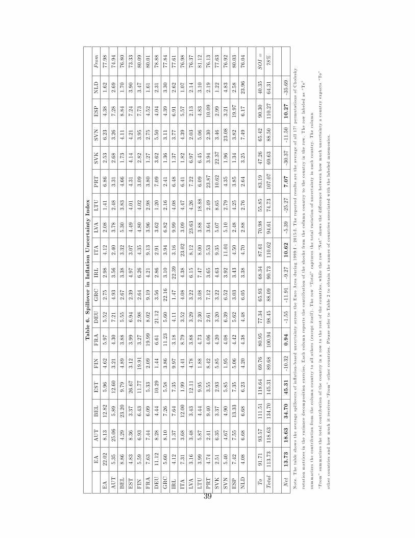
Table6.SpilloverinIn�ationUncertaintyIndex

EA

AUT

BEL

EST

FIN

FRA

DEU

GRC

IRL

ITA

LVA

LTU

PRT

SVK

SVN

ESP

NLD

From

EA

22.02

8.13

12.82

5.96

4.62

5.97

5.52

2.75

2.98

4.12

2.08

1.41

6.86

2.53

6.23

4.38

1.62

77.98

AUT

5.35

25.06

5.89

12.60

3.21

4.30

7.21

4.93

3.56

2.40

3.78

2.48

3.31

2.68

3.26

7.28

2.69

74.94

BEL

8.86

4.29

23.20

9.79

4.89

3.88

5.55

2.67

3.38

3.32

5.30

3.83

4.66

1.73

4.11

8.84

1.70

76.80

EST

4.83

8.36

3.37

26.67

3.12

3.99

6.94

2.39

4.97

3.07

4.49

4.01

4.31

4.14

4.21

7.24

3.90

73.33

FIN

5.59

6.93

6.43

11.77

19.91

3.27

2.98

2.64

6.26

4.35

4.80

4.02

3.09

2.82

3.95

7.73

3.47

80.09

FRA

7.63

7.44

6.09

5.33

2.09

19.99

8.02

9.19

4.21

9.13

3.96

2.98

3.80

1.27

2.75

4.52

1.61

80.01

DEU

11.12

8.28

4.44

10.29

1.44

6.61

21.12

3.56

2.86

2.91

3.62

1.20

7.09

3.62

5.50

4.04

2.31

78.88

GRC

5.60

8.10

7.26

5.58

3.86

11.23

5.60

22.16

3.10

3.94

6.82

2.16

2.41

1.36

3.11

4.39

3.30

77.84

IRL

4.12

1.37

7.64

7.35

9.97

3.18

4.11

1.47

22.39

3.16

9.99

4.08

6.48

1.37

3.77

6.91

2.62

77.61

ITA

7.31

3.68

12.00

1.99

4.41

8.79

3.52

4.08

4.38

23.02

3.09

4.47

6.41

1.82

4.39

5.57

1.07

76.98

LVA

3.16

3.48

3.43

12.11

4.78

3.88

3.29

3.22

6.15

8.12

23.63

4.26

7.22

6.97

2.03

2.13

2.14

76.37

LTU

3.99

5.87

4.44

9.95

1.88

4.73

2.30

3.08

7.47

8.00

3.88

18.88

6.09

6.45

5.06

4.83

3.10

81.12

PRT

4.74

2.41

9.40

3.55

8.42

4.06

2.61

7.12

3.65

5.53

3.64

2.49

23.87

3.94

2.30

10.09

2.19

76.13

SVK

2.51

6.35

3.37

2.93

5.85

4.20

3.20

3.22

4.63

9.35

5.07

8.65

10.62

22.37

3.46

2.99

1.22

77.63

SVN

5.40

4.67

4.90

5.85

1.95

4.08

6.39

6.52

3.92

11.01

5.10

2.79

4.35

1.96

23.08

3.21

4.83

76.92

ESP

7.42

7.55

13.33

7.35

5.06

4.42

5.62

3.03

3.43

4.50

2.48

4.25

3.85

1.34

3.82

19.97

2.58

80.03

NLD

4.08

6.68

6.68

6.23

4.20

4.38

4.48

6.05

3.38

4.70

2.88

2.76

2.64

3.25

7.49

6.17

23.96

76.04

To

91.71

93.57

111.51

118.64

69.76

80.95

77.34

65.93

68.34

87.61

70.98

55.85

83.19

47.26

65.42

90.30

40.35

SOI=

Total

113.73

118.63

134.70

145.31

89.68

100.94

98.45

88.09

90.73

110.62

94.61

74.73

107.07

69.63

88.50

110.27

64.31

78%

Net

13.73

18.63

34.70

45.31

-10.32

0.94

-1.55

-11.91

-9.27

10.62

-5.39

-25.27

7.07

-30.37

-11.50

10.27

-35.69

Note.Thetableshowstheaveragespilloversofin�ation-baseduncertainty

acrosstheEuro

Areaduring1999:I-2015:I.Thereported

resultsaretheaverageofall17!permutationsofCholesky

rotationmatricesinthevariance

decompositionexercise.Each

columnreportsthecontributionoftheshocksfromthecolumncountryto

thecountryintherow.Therowlabeled

as�To�

summarizesthecontributionfromthecolumncountryto

allothers(exceptitself).Therow�Total�capturesthetotalvariationofuncertainty

ineach

country.Thecolumn

�From�summarizesthetotalcontributionofthecountryinarowto

therestofthecountries,whiletherow�Net�showsthedi¤erence

betweenhowmuch

uncertainty

acountryexports�To�

othercountriesandhowmuch

itreceives�From�othercountries.Pleasereferto

Table2to

obtainthenamesofcountriesassociatedwiththelabeled

mnem

onics.

39

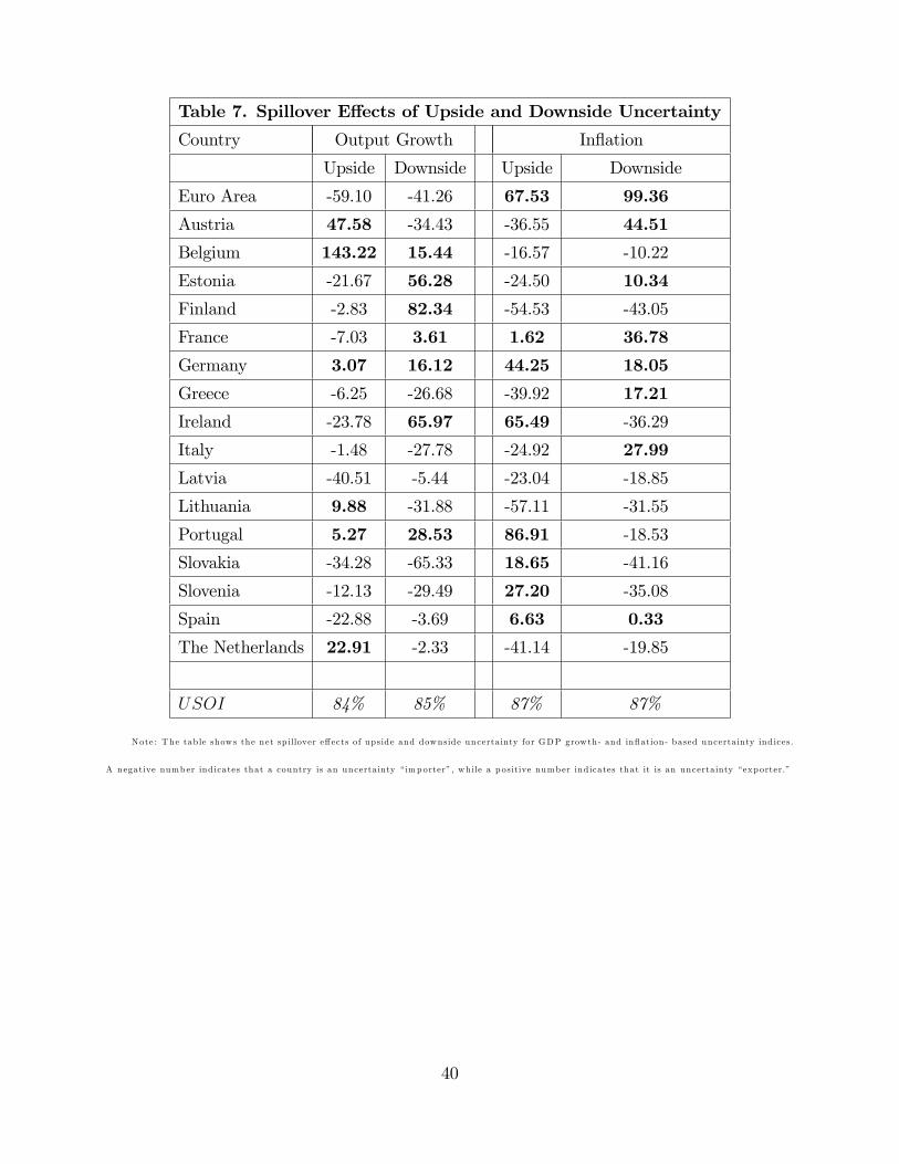
Table 7. Spillover E¤ects of Upside and Downside Uncertainty

Country Output Growth In�ation

Upside Downside Upside Downside

Euro Area -59.10 -41.26 67.53 99.36

Austria 47.58 -34.43 -36.55 44.51

Belgium 143.22 15.44 -16.57 -10.22

Estonia -21.67 56.28 -24.50 10.34

Finland -2.83 82.34 -54.53 -43.05

France -7.03 3.61 1.62 36.78

Germany 3.07 16.12 44.25 18.05

Greece -6.25 -26.68 -39.92 17.21

Ireland -23.78 65.97 65.49 -36.29

Italy -1.48 -27.78 -24.92 27.99

Latvia -40.51 -5.44 -23.04 -18.85

Lithuania 9.88 -31.88 -57.11 -31.55

Portugal 5.27 28.53 86.91 -18.53

Slovakia -34.28 -65.33 18.65 -41.16

Slovenia -12.13 -29.49 27.20 -35.08

Spain -22.88 -3.69 6.63 0.33

The Netherlands 22.91 -2.33 -41.14 -19.85

USOI 84% 85% 87% 87%

Note: The tab le shows the net sp illover e¤ects of upside and downside uncerta inty for GDP growth- and in�ation- based uncerta inty ind ices.

A negative number ind icates that a country is an uncerta inty �importer�, while a p ositive number ind icates that it is an uncerta inty �exporter.�

40

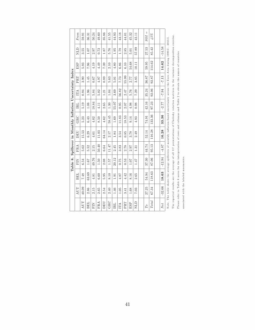
Table8.SpilloverinMonthlyIn�ationUncertaintyIndex

AUT

BEL

FIN

FRA

DEU

GRC

IRL

ITA

PRT

ESP

NLD

From

AUT

40.09

7.48

6.54

5.62

15.53

5.23

5.19

0.94

3.90

5.93

3.55

59.91

BEL

2.86

63.69

1.67

5.52

6.29

6.43

1.08

1.96

1.45

7.96

1.07

36.31

FIN

2.15

4.81

49.76

2.15

4.61

4.02

18.84

5.84

0.67

4.19

2.97

50.24

FRA

2.65

6.60

1.50

50.40

11.03

8.50

4.11

5.02

4.97

4.49

0.72

49.60

DEU

2.54

5.95

2.08

6.64

64.14

4.62

2.65

1.21

0.89

7.39

1.87

35.86

GRC

2.40

8.10

1.57

11.47

2.17

58.45

1.30

1.04

5.63

2.10

5.76

41.55

IRL

1.46

1.91

20.12

2.45

1.84

1.69

55.07

3.69

5.01

4.80

1.95

44.93

ITA

1.05

4.87

0.75

3.83

3.54

11.83

0.95

56.82

7.73

6.86

1.78

43.18

PRT

3.41

4.42

0.53

2.78

0.85

18.53

2.07

2.47

55.99

6.10

2.85

44.01

ESP

1.68

8.16

1.07

2.97

3.78

9.14

4.98

5.76

2.77

54.68

5.01

45.32

NLD

7.03

2.65

1.47

1.31

2.49

4.93

0.98

7.29

3.85

10.11

57.89

42.11

To

27.25

54.94

37.30

44.74

52.14

74.91

42.16

35.24

36.87

59.95

27.53

SOI=

Total

67.34

118.63

87.06

95.13

116.28

133.36

97.23

92.06

92.87

114.62

85.42

45%

Net

-32.66

18.63

-12.94

-4.87

16.28

33.36

-2.77

-7.94

-7.13

14.62

-14.58

Note.Thetableshowstheaveragespilloversofmonthlyin�ation-baseduncertainty

acrosstheEuro

Areaduring1999:I-2015:I.

Thereported

resultsaretheaverageofall11!permutationsofCholeskyrotationmatricesinthevariance

decompositionexercise.

Pleasereferto

Table6notesfortheinterpretationofrowsandcolumnsandTable2to

obtainthenamesofcountries

associatedwiththelabeled

mnem

onics.

41