Embed Size (px)
Citation preview
HAL Id: hal-01656264https://hal.inria.fr/hal-01656264
Submitted on 5 Dec 2017
HAL is a multi-disciplinary open accessarchive for the deposit and dissemination of sci-entific research documents, whether they are pub-lished or not. The documents may come fromteaching and research institutions in France orabroad, or from public or private research centers.
L’archive ouverte pluridisciplinaire HAL, estdestinée au dépôt et à la diffusion de documentsscientifiques de niveau recherche, publiés ou non,émanant des établissements d’enseignement et derecherche français ou étrangers, des laboratoirespublics ou privés.
Distributed under a Creative Commons Attribution| 4.0 International License
Share Market Sectoral Indices Movement Forecast withLagged Correlation and Association Rule Mining
Giridhar Maji, Soumya Sen, Amitrajit Sarkar
To cite this version:Giridhar Maji, Soumya Sen, Amitrajit Sarkar. Share Market Sectoral Indices Movement Forecast withLagged Correlation and Association Rule Mining. 16th IFIP International Conference on ComputerInformation Systems and Industrial Management (CISIM), Jun 2017, Bialystok, Poland. pp.327-340,�10.1007/978-3-319-59105-6_28�. �hal-01656264�
Share Market Sectoral Indices Movement Forecast with
Lagged Correlation and Association Rule Mining
Giridhar Maji1, Soumya Sen
2 and Amitrajit Sarkar
3
1Department of Electrical Engineering, Asansol Polytechnic, India
[email protected] 2AK Choudhury School of Information Technology, University of Calcutta, Kolkata, India
[email protected] 3Ara Institute of Canterbury, NZ
Abstract. This paper analyses the correlation between two different sectoral in-
dices (e.g. between Automobile sector index and between Metal sector index,
between Bank sector index and IT sectoral index etc.) in a time lagged manner.
Lagging period is varied from 1 day to 5 days to investigate if any selected sec-
tor has lagged influence over any other sectoral index movement. If any up-
ward/downward movement of a sectoral index (sector A) is correlated with sim-
ilar upward/downward movement of another sectoral index (Sector B) with a
time lag of ‗d‘ days, then with association rule mining support and confidence
is calculated for the combination. If d is the lag for which support and confi-
dence is maximum then depending on the higher correlation as well as higher
support and confidence value it is possible to forecast future (d days ahead of
current day) movement of sector B based on present day movement of sector A.
This model first uses correlational analysis to identify the level of dependence
among two different sectors, then considers only those sectors having higher
value of correlation for association rule mining. Those sector are not considered
for which combination correlation is very low or 0.
This model has been tested with Indian share market data (NSE sectoral in-
dex data of 6 sectors) of 2015. Result shows it is possible to predict in short
term (1 to 5 days in future) price movement of sectoral indices using other
lagged correlated sector price index movement.
Keywords: stock indices prediction, lagged correlation, association rule mining
1 Introduction
Predicting the future stock prices are the most important queries for the investors in
share market. Many different techniques, mathematical formulation, genetic algorithm
(GA) based models, neural network models, machine learning based techniques etc.
have been proposed and tested with mixed success[1,2,3,15]. Predicting the future
price of some stock is inherently difficult as the price movement depends on large
number of issues gre tly of macro-economic, micro-economic, technical parameters
as well as a lot of unknown parameters which come in to the context all of a sudden.
Future stock price of a company becomes stochastic due to difference in perception
about the future of the company among investors. A group of investor foresees a fu-
ture uptrend or good earnings for the company and they expect its stock price to go up
in near future. Therefore they buy at current price to sell at some higher price in future
and earn profit. At the same time some other groups of investors with a perception
th t the comp ny‘s future outlook is not so good nd stock prices m y f ll in future,
they sell with current price with a view to latter buy the same or more quantity of
shares with lower price in future to earn profit. The basic idea behind technical analy-
sis is that current stock price of a company incorporates impacts and effects of eco-
nomic, financial, political and psychological factors. It studies the historical stock
prices and assumes that the future trend will follow the past behavior. The technical
analysis offers information about the possible future evolution of the stock market.
Technical analysis is done based on a lot of different technical indicator parameters
such s ‗n-d ys moving ver ge‘ (where ‗n‘ c n be 5/10/20/50 etc. d ys), ‗n-days
weighted ver ge‘, MACD, relative strength index, momentum etc. along with price-
to-earnings ratio, dividend yield, profit margin , return on investment etc.[2,3,12,15].
But investor‘s perception also depends on rumors & market speculation and some
unforeseen sudden big events and their unknown reaction towards stock prices of
different comp nies. This l ter p rt m kes the ―sell‖ or ―buy‖ decision of n investor
a stochastic random event but due to the technical parameters it is also not totally
unpredictable.
In any Stock market listed companies are categorized into different sectors depend-
ing on the business domain the company belongs to. We have considered the follow-
ing six sectors for our study: Banks, Automobiles, IT & Software, Metals, Pharma-
ceuticals and FMCG (Fast Moving Consumer Goods). These different sectors have
sectoral index to represent their aggregated trends in a stock exchange. It is similar to
the stock exchange index (for example SENSEX, NIFTY in BSE and NSE). These
sectoral indices react with different external and internal events differently and hence
their movement. Same external event may affect different industry sector differently.
Depending on a many different factors some sectoral index moves in positive direc-
tion while in the same time some other sector moves into the negative zone (or may
remain neutral). As an example when dollar value increases with respect to Indian
Rupee (INR) almost all export companies of India gains and IT sectors majorly get
most of the benefits as they earn in dollar and spend in INR. At the same time import-
ers incur losses.
This is a very complex relationship to measure. In this research work we aim to fo-
cus on this in terms of following issues:
1. If these reactions with the external factors are correlated between the sectors.
2. Identifying how different sectors are related? They may be highly correlated, corre-
lated, neutral or not co-related at all.
3. Among the highly correlated sector pairs which are positively correlated and which
are negatively correlated.
4. Is there any correlation among the highly correlated sector pairs with some days
l g, i.e. if tod y‘s sectoral index movement of sector-A is correlated with sectoral
index movement of sector-B on d days in future. If we find a high correlation
among two different sectors with a time lag of d days then we can forecast sectoral
index movement of Sector-B,‗d‘ days ahead.
In the next sub section we briefly discuss about Indian share market as well as sec-
toral indices that are considered in this case study. Then we will discuss about Asso-
ciation rule mining techniques along with support and confidence that will be used in
our analysis.
An Overview of Indian Share Market
Two most important stock exchanges in India are BSE and NSE. The Bombay
Stock Exchange (BSE) is one of the oldest stock exchanges in India and one of the
top stock exchanges globally with respect to number of listed companies and market
capitalization. The 30 company index from BSE is known as SENSEX or BSE30 is a
stock market index of 30 well established and financially sound companies listed on
BSE. These are some of the largest and most actively traded stocks, hence it is con-
sidered as representative of various industrial sectors of the Indian economy. It is
published since 1st January 1986 and regarded as the pulse of the domestic stock
markets in India [9]. The NIFTY 50 index is n tion l stock exch nge of Indi ‘s
benchmark stock market index for Indian equity market [10]. It covers 22 sectors of
Indian economy. As SENSEX and NIFTY is used to understand average trend and
movement of BSE and NSE for almost all financial purposes, each stock exchange
has industry sectors and each sector has many sectoral index(s) that reflect the behav-
ior and performance of the concerned sector. In this study following 6 sectors are
considered: Auto, Bank, Pharma, FMCG, IT and Metal. All index values are taken
from NIFTY industrial sectors. Different sectoral index(s) consists of different num-
ber of representative company stocks. For example NSE Auto Index consists of 15
stocks and NIFTY bank index comprises of 12 banking sector stocks.
Statistical Correlation
Let Xt and Yt are two given time series closing prices for N days. If we consider a
lag of d days between them then co-variance between the two series is defined as-
∑
where μX and μY are the sample means of the time series X and Y.
Cross correlation between them is defined as-
Where x , and Y ;
Sx , Sy being the sample standard deviations of series X and Y.
The value of r varies between +1 to -1. Depending on the sign of r following can be
inferred:
Positive correlation: r value closer to +1 signifies strong positive correlation be-
tween the variables. An r value of exact +1 indicates a perfect positive fit. Any
positive r values between 0 and +1 indicates that the relationship between x and y
variables are such that with increase in values of X, Y value also increases.
Negative correlation: If x and y have a strong negative linear correlation, r is close
to an r value of exactly -1 indicates a perfect negative fit. Negative values indicate
a relationship between x and y such that as values for x increase, values for y de-
crease.
No correlation: r value closer to 0 signifies that there is no linear correlation or a
very weak correlation. In other words x and y values are completely un-correlated
and there is a random, relationship between the two variables x, y.
A perfect correlation of ± 1means that all the data points are lying on a straight
line. Correlation coefficient ‗r‘ does not have a dimension; hence it does not depend
on the units used. Generally an ‗r‘ value of greater than 0.8 is considered as highly
correlated and less than 0.5 is considered weakly correlated. A point to remember is
th t bove threshold v lues v ry with the ‗type‘ of d t used. Gener lly with noisy
data less threshold values are considered.
Association Rule Mining
Data mining, an important part of knowledge discovery in databases (KDD) pro-
cess employs many different techniques for knowledge discovery and prediction such
as classification, clustering, sequential pattern mining, association rule mining and
analysis. Nowadays it is used in almost all the data driven decision models such as
business analysis, strategic decision making, financial forecasting, future sales predic-
tion etc. Agrawal [13] first introduced association rules for frequent pattern mining
among items in large transaction dataset. They introduced the Apriori principle which
says: Any subset of a frequent itemset must be frequent. Hence it can also be said in
another term as: No superset of any infrequent itemset should be calculated for further
processing. From the frequent item-sets a set of strong rules are calculated. Strength
of a rule is measured based on support and confidence values. Not all frequent item-
sets are considered as strong, only those with a minimum support and confidence are
considered for the next step. This Aprori principle elimin tes the ‗curse of dimension-
lity‘ nd m kes computations feasible. Let us consider an association rule :{ bread,
sugar} => {butter} It indicates if people are buying bread and sugar then they may
also buy butter. Association rule mining (ARM) is used here to show the relationship
between different item-sets. It is also known as market basket analysis. An association
rule is expressed in the form of an implication as:
X → Y, where X and Y are disjoint item-sets, i.e. ∩ Y = ∅.
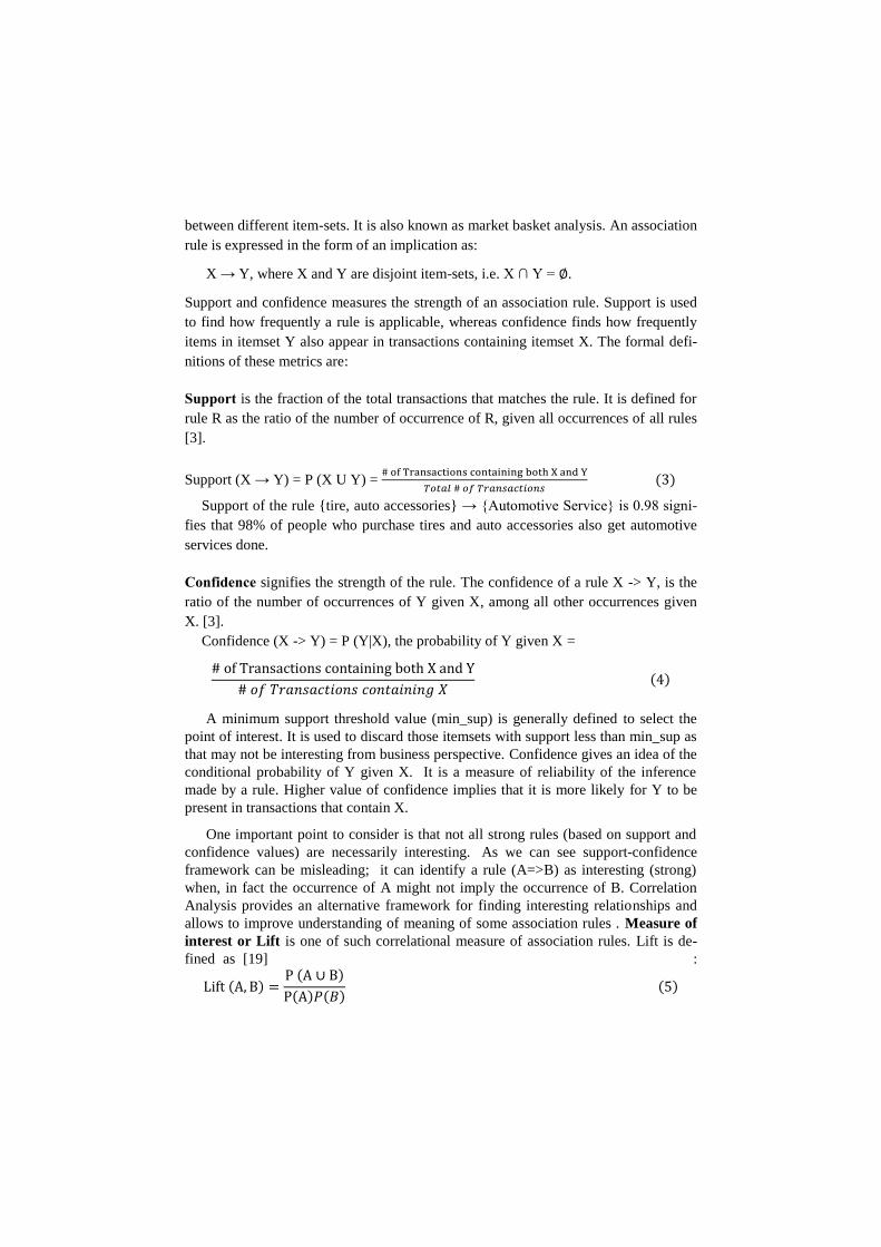
Support and confidence measures the strength of an association rule. Support is used
to find how frequently a rule is applicable, whereas confidence finds how frequently
items in itemset Y also appear in transactions containing itemset X. The formal defi-
nitions of these metrics are:
Support is the fraction of the total transactions that matches the rule. It is defined for
rule R as the ratio of the number of occurrence of R, given all occurrences of all rules
[3].
Support (X → Y) = P (X U Y) =
Support of the rule {tire, auto accessories} → {Automotive Service} is 0.98 signi-
fies that 98% of people who purchase tires and auto accessories also get automotive
services done.
Confidence signifies the strength of the rule. The confidence of a rule X -> Y, is the
ratio of the number of occurrences of Y given X, among all other occurrences given
X. [3].
Confidence (X -> Y) = P (Y|X), the probability of Y given X =
A minimum support threshold value (min_sup) is generally defined to select the
point of interest. It is used to discard those itemsets with support less than min_sup as
that may not be interesting from business perspective. Confidence gives an idea of the
conditional probability of Y given X. It is a measure of reliability of the inference
made by a rule. Higher value of confidence implies that it is more likely for Y to be
present in transactions that contain X.
One important point to consider is that not all strong rules (based on support and
confidence values) are necessarily interesting. As we can see support-confidence
framework can be misleading; it can identify a rule (A=>B) as interesting (strong)
when, in fact the occurrence of A might not imply the occurrence of B. Correlation
Analysis provides an alternative framework for finding interesting relationships and
allows to improve understanding of meaning of some association rules . Measure of
interest or Lift is one of such correlational measure of association rules. Lift is de-
fined as [19] :
If lift = 1 i.e. P (AꓴB) = P (A) P (B) , then the occurrence of itemset A is independ-
ent of the occurrence of B; or else both the item-sets are dependent and correlated. If
lift value is less than 1 then A and B are negatively correlated i.e. occurrence of one
likely implies the absence of the other. A lift value of more than 1 implies positive
correlation between A and B.
2 Related Study
Several researches have been done over the period on predicting future stock price or
price movement direction (upward or downward) along with trend analysis based on
mainly different statistical modeling [3,4,6,7,8,14,15]. Rusu et al. discussed stock
forecasting [14] methods used by classical approaches such as fundamentalists and
chartists and at the same time discussed various recent stochastic methods like white
noise, random walk, auto-regressive models etc. In another research work [4] various
models used for stock price prediction using SAS© System tools. Models like Time
Series analysis, Auto Regression (AR), Exponential Smoothening, Moving Average
(MA) etc. has been discussed along with illustrated procedure for FORECAST and
ARIMA (Autoregressive Integrated Moving Average) models. Dutta et al. [15] used
logistic regression methods with various financial ratios as independent variables to
cluster selected 30 stocks into good and bad performing groups based on rate of re-
turn. Another model CARIMA [5] (Cross Correlation Autoregressive Integrated Mov-
ing Average) was proposed to predict short term stock price. Main idea of CARIMA
is to find the most highly correlated stock to predict the target price. Stock prices of
SET50 from Stock Exchange of Thailand has been used to test the effectiveness of the
model with better price trend prediction with similar % MAE (Mean Absolute Error)
than ARIMA model. In another study work authors investigated stock index co-
movement between two different countries namely Taiwan and Hong Kong using
association rules and cluster analysis [6]. They have used 30 categories of stock indi-
ces as decision variables to observe the behavior of stock index association. This
study tried to identify the correlation between the similar category sectoral index
movements between two different countries and that also used to recommend invest-
ment portfolio as a follow up reference. Forecasting horizon is the time lag between
the price movement of independent stock price and correlated stock price. If two
stocks are highly correlated with a delay of d days then following the trend of former
stock, l tter one‘s trend c n be predicted d d ys he d. The bove method is proposed
with suitable generic algorithm for automated data preprocessing and analysis using
correlation [8]. This model has predicted with 67% accuracy while tested with real
stock market data. Authors in [16] has analyzed correlation between stock price fluc-
tuation, gold price and US dollar price along with association rule induction methods
amongst different stocks of same sector. A rigorous mathematical discussion on ten
different data mining techniques such as Support vector machine (SVM), Least
squares support vector machine (LS-SVM), Linear discriminant analysis (LDA),
Quadratic discriminant analysis (QDA), Logit model, neural network, Bayesian mod-
els etc. has been discussed in [17]. In another work authors proposed and evaluated a
stock price prediction based recommender system [18] that used historical stock pric-
es as input to the system and applied regression trees for dimensionality reduction and
Self Organizing Maps (SOM) for clustering. The proposed system helped investors
with possible profit-making opportunities with buy or sell recommendations.
The main objective of this research work is to measure the association between
sectors pair-wise instead of specific stock. These would provide an integrated view of
stock market including several business sectors. Here we study time lagged prediction
model for the analysis on the well-established, industry defined sectors or domains of
businesses like automobile, banking, reality, metal etc. As we identify the sectors
instead of specific stock we able to consider number of stocks at a time and could
choose the top performing stocks of the sector as required. The sectoral index of each
sector has been used to find the correlation in our study. This way total number of
possible sector pair reduces drastically and at the same time individual investors can
gain an idea to which sectoral stocks are going to give good earning in short-term.
Similarly mutual fund managers can also use it to diversify their sectoral portfolio as
the movement trend of sectors is going to be identified.
3 Methodology
Research Framework
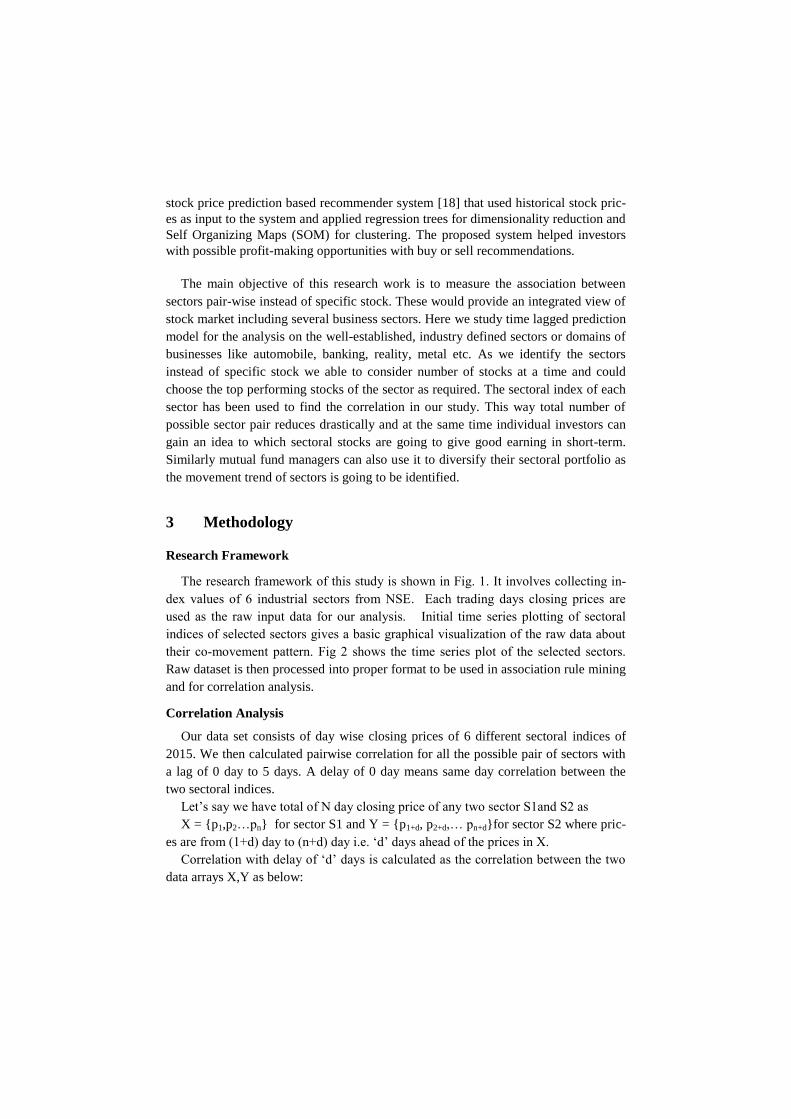
The research framework of this study is shown in Fig. 1. It involves collecting in-
dex values of 6 industrial sectors from NSE. Each trading days closing prices are
used as the raw input data for our analysis. Initial time series plotting of sectoral
indices of selected sectors gives a basic graphical visualization of the raw data about
their co-movement pattern. Fig 2 shows the time series plot of the selected sectors.
Raw dataset is then processed into proper format to be used in association rule mining
and for correlation analysis.
Correlation Analysis
Our data set consists of day wise closing prices of 6 different sectoral indices of
2015. We then calculated pairwise correlation for all the possible pair of sectors with
a lag of 0 day to 5 days. A delay of 0 day means same day correlation between the
two sectoral indices.
Let‘s s y we h ve tot l of N d y closing price of ny two sector S1 nd S2 s
X = {p1,p2…pn} for sector S1 and Y = {p1+d, p2+d,… pn+d}for sector S2 where pric-
es are from (1+d) d y to (n+d) d y i.e. ‗d‘ d ys he d of the prices in .
Correl tion with del y of ‗d‘ d ys is c lcul ted s the correl tion between the two
data arrays X,Y as below:
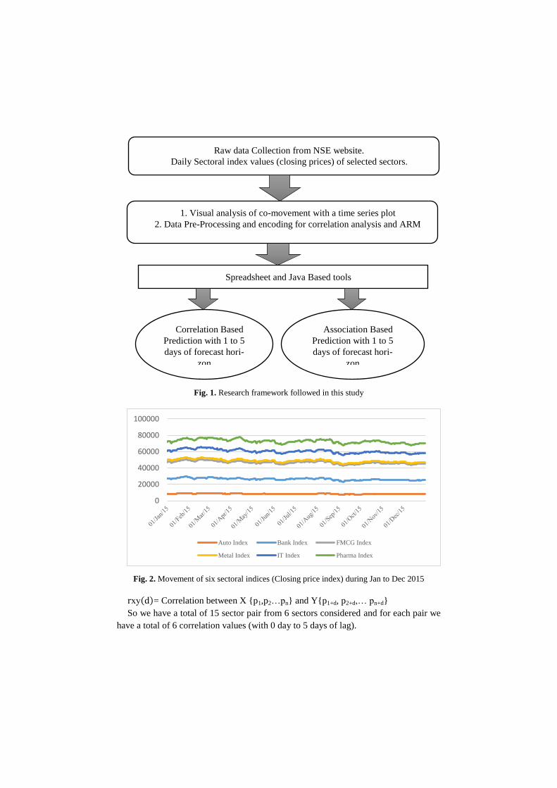
Fig. 1. Research framework followed in this study
Fig. 2. Movement of six sectoral indices (Closing price index) during Jan to Dec 2015
xy = Correlation between X {p1,p2…pn} and Y{p1+d, p2+d,… pn+d}
So we have a total of 15 sector pair from 6 sectors considered and for each pair we
have a total of 6 correlation values (with 0 day to 5 days of lag).
0
20000
40000
60000
80000
100000
Auto Index Bank Index FMCG Index
Metal Index IT Index Pharma Index
Raw data Collection from NSE website.
Daily Sectoral index values (closing prices) of selected sectors.
1. Visual analysis of co-movement with a time series plot
2. Data Pre-Processing and encoding for correlation analysis and ARM
Correlation Based
Prediction with 1 to 5
days of forecast hori-
zon
Association Based
Prediction with 1 to 5
days of forecast hori-
zon
Spreadsheet and Java Based tools
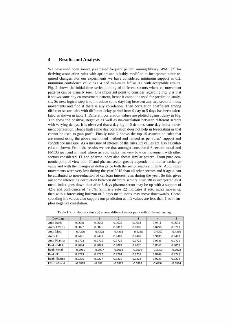
Microsoft excel spreadsheet based statistical tools has been used to derive the re-
sults shown in table 1 and Fig. 3.
In this study a correlation value of r >=0.8 has been considered as good correlation
nd correl tion v lue of r<=0.5 h s been neglected s ‗we k or no correl tion‘.
Based on the correlation between different sectoral movements sector pairs are select-
ed for further analysis using association rule mining. Only sector pairs with high posi-
tive or negative correlation are considered for further analysis as discussed in the next
sub section.
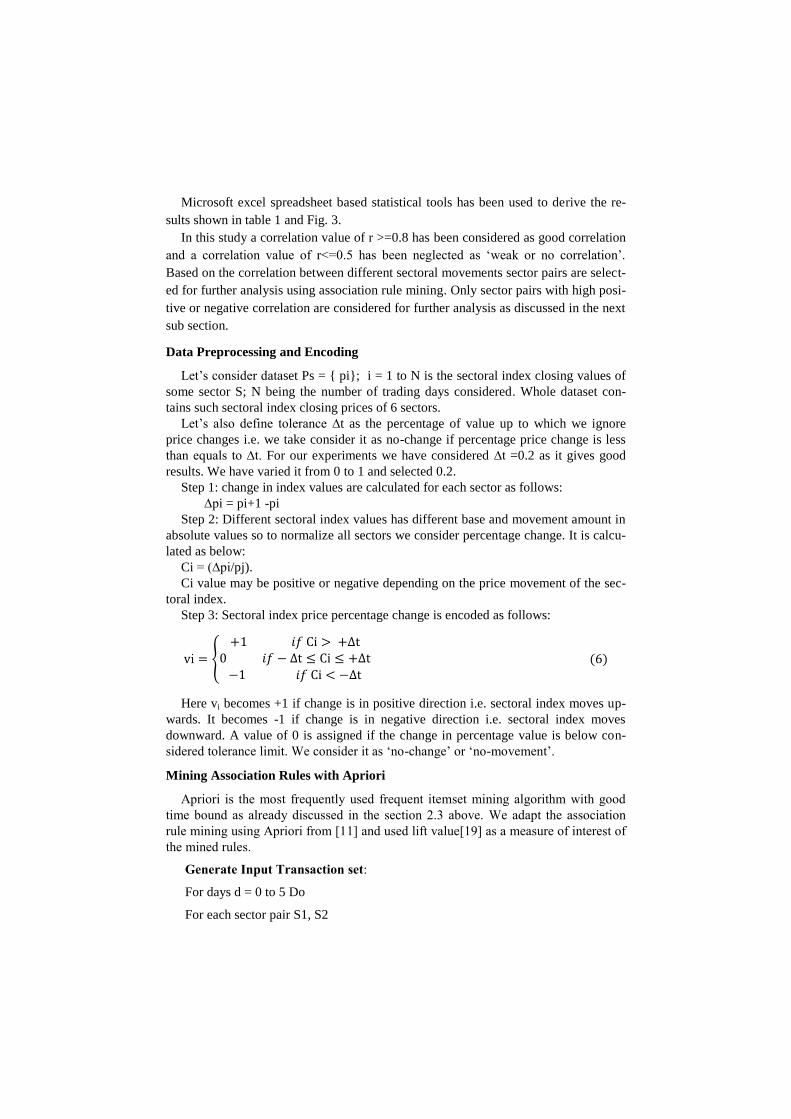
Data Preprocessing and Encoding
Let‘s consider d t set Ps = { pi}; i = 1 to N is the sectoral index closing values of
some sector S; N being the number of trading days considered. Whole dataset con-
tains such sectoral index closing prices of 6 sectors.
Let‘s lso define toler nce ∆t as the percentage of value up to which we ignore
price changes i.e. we take consider it as no-change if percentage price change is less
th n equ ls to ∆t. For our experiments we have considered ∆t =0.2 as it gives good
results. We have varied it from 0 to 1 and selected 0.2.
Step 1: change in index values are calculated for each sector as follows:
∆pi = pi+1 -pi
Step 2: Different sectoral index values has different base and movement amount in
absolute values so to normalize all sectors we consider percentage change. It is calcu-
lated as below:
Ci = (∆pi/pj).
Ci value may be positive or negative depending on the price movement of the sec-
toral index.
Step 3: Sectoral index price percentage change is encoded as follows:
{
Here vi becomes +1 if change is in positive direction i.e. sectoral index moves up-
wards. It becomes -1 if change is in negative direction i.e. sectoral index moves
downward. A value of 0 is assigned if the change in percentage value is below con-
sidered toler nce limit. We consider it s ‗no-ch nge‘ or ‗no-movement‘.
Mining Association Rules with Apriori
Apriori is the most frequently used frequent itemset mining algorithm with good
time bound as already discussed in the section 2.3 above. We adapt the association
rule mining using Apriori from [11] and used lift value[19] as a measure of interest of
the mined rules.
Generate Input Transaction set:
For days d = 0 to 5 Do
For each sector pair S1, S2
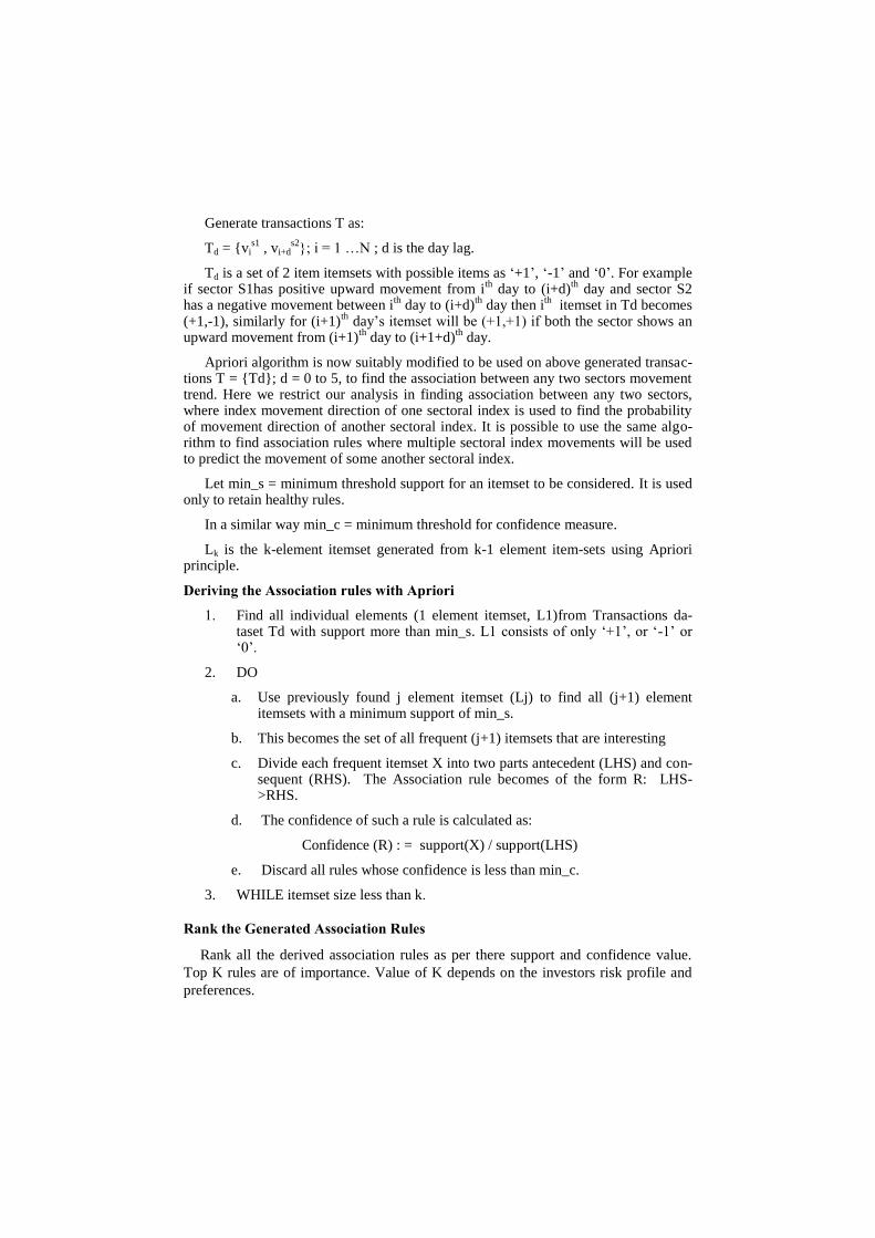
Generate transactions T as:
Td = {vis1
, vi+ds2}; i = 1 …N ; d is the day lag.
Td is a set of 2 item itemsets with possible items as ‗+1‘, ‗-1‘ and ‗0‘. For example if sector S1has positive upward movement from i
th day to (i+d)
th day and sector S2
has a negative movement between ith
day to (i+d)th
day then ith
itemset in Td becomes (+1,-1), similarly for (i+1)
th day‘s itemset will be (+1,+1) if both the sector shows an
upward movement from (i+1)th
day to (i+1+d)th
day.
Apriori algorithm is now suitably modified to be used on above generated transac-tions T = {Td}; d = 0 to 5, to find the association between any two sectors movement trend. Here we restrict our analysis in finding association between any two sectors, where index movement direction of one sectoral index is used to find the probability of movement direction of another sectoral index. It is possible to use the same algo-rithm to find association rules where multiple sectoral index movements will be used to predict the movement of some another sectoral index.
Let min_s = minimum threshold support for an itemset to be considered. It is used only to retain healthy rules.
In a similar way min_c = minimum threshold for confidence measure.
Lk is the k-element itemset generated from k-1 element item-sets using Apriori principle.
Deriving the Association rules with Apriori
1. Find all individual elements (1 element itemset, L1)from Transactions da-taset Td with support more than min_s. L1 consists of only ‗+1‘, or ‗-1‘ or ‗0‘.
2. DO
a. Use previously found j element itemset (Lj) to find all (j+1) element itemsets with a minimum support of min_s.
b. This becomes the set of all frequent (j+1) itemsets that are interesting
c. Divide each frequent itemset X into two parts antecedent (LHS) and con-sequent (RHS). The Association rule becomes of the form R: LHS->RHS.
d. The confidence of such a rule is calculated as:
Confidence (R) : = support(X) / support(LHS)
e. Discard all rules whose confidence is less than min_c.
3. WHILE itemset size less than k.
Rank the Generated Association Rules
Rank all the derived association rules as per there support and confidence value.
Top K rules are of importance. Value of K depends on the investors risk profile and
preferences.
4 Results and Analysis
We have used open source java based frequent pattern mining library SPMF [7] for
deriving association rules with apriori and suitably modified to incorporate other re-
quired changes. For our experiments we have considered minimum support as 0.2,
minimum confidence value as 0.4 and minimum lift as 0.1 with acceptable results.
Fig. 2 shows the initial time series plotting of different sectors where co-movement
patterns can be visually seen. One important point to consider regarding Fig. 2 is that
it shows same day co-movement pattern, hence it cannot be used for prediction analy-
sis. So next logical step is to introduce some days lag between any two sectoral index
movements and find if there is any correlation. Then correlation coefficient among
different sector pairs with different delay period from 0 day to 5 days has been calcu-
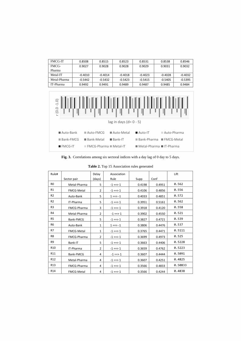
lated as shown in table 1. Different correlation values are plotted against delay in Fig.
3 to show the positive, negative as well as no-correlation between different sectors
with varying delays. It is observed that a day lag of 0 denotes same day index move-
ment correlation. Hence high same day correlation does not help in forecasting as that
cannot be used to gain profit. Finally table 2 shows the top 15 association rules that
re mined using the bove mentioned method nd r nked s per rules‘ support nd
confidence measure. As a measure of interest of the rules lift values are also calculat-
ed and shown. From the results we see that amongst considered 6 sectors metal and
FMCG go hand in hand where as auto index has very low co movement with other
sectors considered. IT and pharma index also shows similar pattern. From pure eco-
nomic point of view both IT and pharma sector greatly dependent on dollar exchange
value and with the changes in dollar price both the sector reacts similarly. Auto index
movements were very low during the year 2015 than all other sectors and it again can
be attributed to non-reduction of car loan interest rates during the year. So this gives
out some interesting correlation between different sectors. Rule R0 is interpreted as if
metal index goes down then after 5 days pharma sector may be up with a support of
42% and confidence of 49.5%. Similarly rule R2 indicates if auto index moves up
then with a forecasting horizon of 5 days metal index may move downwards. Corre-
sponding lift values also support our prediction as lift values are less than 1 so it im-
plies negative correlation.
Table 1. Correlation values (r) among different sector pairs with different day lag.
Day Lag-> 0 1 2 3 4 5
Auto-Bank 0.9638 0.9633 0.9625 0.9618 0.9611 0.9604
Auto- FMCG 0.8827 0.8821 0.8813 0.8805 0.8796 0.8787
Auto-Metal -0.4220 -0.4228 -0.4238 - 0.4248 -0.4257 -0.4266
Auto- IT 0.9491 0.9491 0.9489 0.9488 0.9485 0.9482
Auto-Pharma 0.9723 0.9725 0.9725 0.9725 0.9725 0.9725
Bank-FMCG 0.8094 0.8089 0.8083 0.8076 0.8067 0.8058
Bank-Metal -0.2981 -0.2997 -0.3018 -0.3039 -0.3059 -0.3078
Bank-IT 0.8779 0.8772 0.8764 0.8757 0.8748 0.8741
Bank-Pharma 0.9226 0.9227 0.9226 0.9224 0.9223 0.9222
FMCG-Metal -0.6889 -0.6891 -0.6892 -0.6893 -0.6894 -0.6894
FMCG-IT 0.8508 0.8515 0.8523 0.8531 0.8538 0.8546
FMCG-
Pharma
0.9027 0.9028 0.9028 0.9029 0.9031 0.9032
Metal-IT -0.4010 -0.4014 -0.4018 -0.4023 -0.4028 -0.4032
Metal-Pharma -0.5442 -0.5432 -0.5423 -0.5415 -0.5405 -0.5395
IT-Pharma 0.9492 0.9491 0.9489 0.9487 0.9485 0.9484
Fig. 3. Correlations among six sectoral indices with a day lag of 0 day to 5 days.
Table 2. Top 15 Association rules generated
Rule#
Sector pair
Delay
(days)
Association
Rule Supp Conf
Lift
R0 Metal-Pharma 5 -1 ==> 1 0.4198 0.4951 0.562
R1 FMCG-Metal 2 -1 ==> 1 0.4106 0.4856 0.556
R2 Auto-Bank 5 1 ==> -1 0.4033 0.4851 0.572
R2 IT-Pharma 5 -1 ==> 1 0.3951 0.5161 0.562
R3 FMCG-Pharma 3 -1 ==> 1 0.3918 0.4120 0.558
R4 Metal-Pharma 2 -1 ==> 1 0.3902 0.4550 0.521
R5 Bank-FMCG 5 -1 ==> 1 0.3827 0.4721 0.539
R6 Auto-Bank 1 1 ==> -1 0.3806 0.4476 0.537
R7 FMCG-Metal 1 -1 ==> 1 0.3765 0.4471 0.5111
R8 FMCG-Pharma 2 -1 ==> 1 0.3699 0.4973 0.525
R9 Bank-IT 5 -1 ==> 1 0.3663 0.4406 0.5228
R10 IT-Pharma 2 -1 ==> 1 0.3659 0.4762 0.5223
R11 Bank-FMCG 4 -1 ==> 1 0.3607 0.4444 0.5091
R12 Metal-Pharma 4 -1 ==> 1 0.3607 0.4251 0.4825
R13 FMCG-Pharma 4 -1 ==> 1 0.3566 0.4833 0.50833
R14 FMCG-Metal 4 -1 ==> 1 0.3566 0.4244 0.4838
r (0
.0 -
1.0
)
lag in days (d= 0 - 5)
Auto-Bank Auto-FMCG Auto-Metal Auto-IT Auto-Pharma
Bank-FMCG Bank-Metal Bank-IT Bank-Pharma FMCG-Metal
FMCG-IT FMCG-Pharma Metal-IT Metal-Pharma IT-Pharma
5 Conclusion and Future work
Association rule mining along with statistical correlation analysis has been applied on
sectoral index dataset to investigate co-movement patterns among them. Aprori algo-
rithm, a well-known frequent itemset mining tool has been modified and applied for
the present analysis. This study finds that different sectoral indices are correlated
among themselves. One more interesting finding is that there exists a time delayed
lagged correlation between different sectoral indices. This correlation can be exploit-
ed to predict the future index movement direction with a forecast horizon of d days
where d is the number of day lag considered. Hence this model can be used by differ-
ent investors in balancing their portfolio to minimize risk as well as in deciding which
sector to invest next. This model can be considered for short term investment as only
prediction of next few d ys is possible using current d y‘s sector l index movements.
Results shows that some sectors are completely un-correlated but some are highly
correlated (positively or negatively) with correlation coefficient values more than 0.8.
Future work will include analysis considering all sectors at a time instead of only a
single sector predicts another. For example in this study association rules of the form,
R: S1->S2 is used for simplicity, but in future all possible rules of the form R:
(S1…Sj)-> Sk, where ll other sectors jointly predicts some nother sector‘s move-
ment can be studied. Artificial neural network models can also be considered in com-
bination with association rules to predict the sectoral index movement. In this study
only historical closing values of indices are considered but there are many other fac-
tors and features like trading volume, market capitalization, debt ratio etc. that can be
considered for prediction.
6 References
1. Liu, C., & Malik, H. (2014, July). A new investment strategy based on data mining and
Neural Networks. In Neural Networks (IJCNN), 2014 International Joint Conference on
(pp. 3094-3099). IEEE.
2. Inthachot, M., Boonjing, V., & Intakosum, S. (2016). Artificial Neural Network and
Genetic Algorithm Hybrid Intelligence for Predicting Thai Stock Price Index Trend.
Computational Intelligence and Neuroscience, 2016.
3. de Oliveira, F. A., Nobre, C. N., & Zárate, L. E. (2013). Applying Artificial Neural
Networks to prediction of stock price and improvement of the directional prediction
index–Case study of PETR4, Petrobras, Brazil. Expert Systems with Applications, 40(18),
7596-7606.
4. Reddy, B. S. (2010, September). Prediction of Stock Market indices—Using SAS. In
Information and Financial Engineering (ICIFE), 2010 2nd IEEE International Conference
on (pp. 112-116). IEEE.
5. Wichaidit, S., & Kittitornkun, S. (2015, November). Predicting SET50 stock prices using
CARIMA (Cross Correlation ARIMA). In Computer Science and Engineering Conference
(ICSEC), 2015 International (pp. 1-4). IEEE.
6. Liao, S. H., & Chou, S. Y. (2013). Data mining investigation of co-movements on the
Taiwan and China stock markets for future investment portfolio. Expert Systems with
Applications, 40(5), 1542-1554.
7. P. Fournier-Viger, A. Gomariz, A. Soltani and T. Gueniche, SPMF: Open-Source Data
Mining Platform, (2013),http://www.philippe-fournier-viger.com/spmf/
8. Fonseka, C., & Liyanage, L. (2008, December). A Data mining algorithm to analyse stock
market data using lagged correlation. In Information and Automation for Sustainability,
2008. ICIAFS 2008. 4th International Conference on (pp. 163-166). IEEE.
9. BSE India, http://www. bseindia.com accessed on January 26, 2017.
10. NSE India, http://www.nseindia.com accessed on January 26, 2017.
11. Dongre, Jugendra, Gend Lai Prajapati, and S. V. Tokekar. "The role of Apriori algorithm
for finding the association rules in Data mining." In Issues and Challenges in Intelligent
Computing Techniques (ICICT), 2014 International Conference on, pp. 657-660. IEEE,
2014
12. Imandoust, S. B., & Bolandraftar, M. (2014). Forecasting the direction of stock market
index movement using three data mining techniques: the case of Tehran Stock Exchange.
International Journal of Engineering Research and Application, ISSN, 2248-9622.
13. Agr w l, R kesh, Tom sz Imieliński, nd Arun Sw mi. "Mining ssoci tion rules between
sets of items in large databases." In Acm sigmod record, vol. 22, no. 2, pp. 207-216. ACM,
1993
14. Rusu, V., and Rusu, C., ―Forec sting methods nd stock m rket n lysis‖. Creative Math,
12(2003) pp. 103-110.
15. Dutta, A., Bandopadhyay, G., & Sengupta, S. (2015). PREDICTION OF STOCK
PERFORMANCE IN INDIAN STOCK MARKET USING LOGISTIC REGRESSION.
International Journal of Business and Information, 7(1).
16. Mahajan, K. S., & Kulkarni, R. V. (2014). APPLICATION OF DATA MINING TOOLS
FOR SELECTED SCRIPTS OF STOCK MARKET. International Journal of Data Mining
& Knowledge Management Process, 4(4), 55.
17. Ou, P., & Wang, H. (2009). Prediction of stock market index movement by ten data
mining techniques. Modern Applied Science, 3(12), 28.
18. Nair, B. B., Kumar, P. S., Sakthivel, N. R., & Vipin, U. (2017). Clustering stock price time
series data to generate stock trading recommendations: An empirical study. Expert
Systems with Applications, 70, 20-36.
19. Brin, S., Motwani, R., Ullman, J. D., & Tsur, S. (1997, June). Dynamic itemset counting
and implication rules for market basket data. In ACM SIGMOD Record (Vol. 26, No. 2,
pp. 255-264). ACM.