Embed Size (px)
Citation preview
Research Discussion Paper
Macroeconomic Consequences of Terms of Trade Episodes, Past and Present
Tim Atkin, Mark Caputo, Tim Robinson and Hao Wang
RDP 2014-01

The Discussion Paper series is intended to make the results of the current economic research within the Reserve Bank available to other economists. Its aim is to present preliminary results of research so as to encourage discussion and comment. Views expressed in this paper are those of the authors and not necessarily those of the Reserve Bank. Use of any results from this paper should clearly attribute the work to the authors and not to the Reserve Bank of Australia.
The contents of this publication shall not be reproduced, sold or distributed without the prior consent of the Reserve Bank of Australia.
ISSN 1320-7229 (Print)
ISSN 1448-5109 (Online)
Macroeconomic Consequences of Terms of Trade Episodes, Past and Present
Tim Atkin, Mark Caputo, Tim Robinson and Hao Wang
Research Discussion Paper 2014-01
January 2014
Economic Analysis Department Reserve Bank of Australia
An earlier version of this paper was presented at the ‘Commodity Price Volatility, Past and Present’ Conference, held on 29–30 November 2012, by the Centre for Economic History, Research School of Economics, and the Centre for Applied Macroeconomic Analysis, Crawford School of Public Policy, at the Australian National University. We thank participants at the conference, those at a seminar at the Reserve Bank of Australia, Laura Berger-Thomson, Leon Berkelmans, Natasha Cassidy, Ellis Connolly, Troy Gill, Alex Heath, Jonathan Kearns and especially Chris Stewart for helpful comments. Any errors are our own. The views expressed in this paper are those of the authors and not necessarily those of the Reserve Bank of Australia.
Authors: atkina, caputom, robinsont and wangh at domain rba.gov.au
Media Office: [email protected]

i
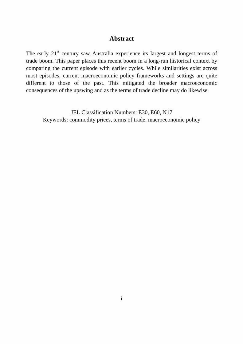
Abstract
The early 21st century saw Australia experience its largest and longest terms of trade boom. This paper places this recent boom in a long-run historical context by comparing the current episode with earlier cycles. While similarities exist across most episodes, current macroeconomic policy frameworks and settings are quite different to those of the past. This mitigated the broader macroeconomic consequences of the upswing and as the terms of trade decline may do likewise.
JEL Classification Numbers: E30, E60, N17 Keywords: commodity prices, terms of trade, macroeconomic policy
ii
Table of Contents
1. Introduction 1
2. Terms of Trade Episodes 3
3. Macroeconomic Consequences 8
3.1 Investment 12
3.2 Trade 13
3.3 Consumption 16
4. Economic Policy Settings and Terms of Trade Episodes 18
4.1 Monetary Policy 18
4.2 Fiscal Policy 22
4.3 Population Policy 26
4.4 Trade Protection 27
4.5 Labour Market 28
5. Conclusions 30
Appendix A: Dating the Terms of Trade 33
Appendix B: Data Sources 34
Appendix C: Economic Indicators around Terms of Trade Peaks 37
References 38
Macroeconomic Consequences of Terms of Trade Episodes, Past and Present
Tim Atkin, Mark Caputo, Tim Robinson and Hao Wang
1. Introduction
The terms of trade – that is, the ratio of export prices to import prices – dictate the real purchasing power of domestic output and are a key determinant of a nation’s economic prosperity. Large movements in the terms of trade can have important macroeconomic implications as relative prices and incomes change.
This paper places the current terms of trade boom in its historical context. It draws on a wide range of long-run macroeconomic and financial data, some of which pre-date Federation, to examine major terms of trade episodes in Australia. The paper highlights differences in the duration and the nature of the shocks driving these episodes. It also documents the prevailing policy settings and compares the macroeconomic outcomes.
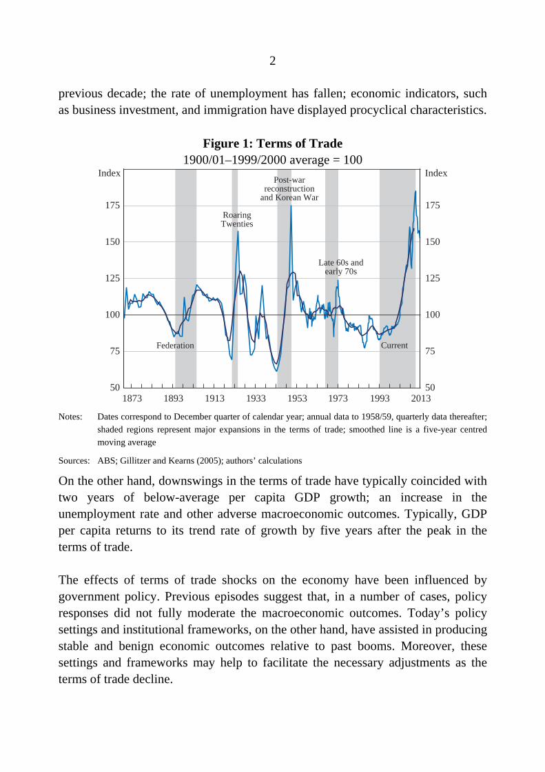
Australia’s terms of trade have increased markedly over the past decade, reaching a peak in September 2011 that was around 85 per cent above the previous century’s average (Figure 1). This is, however, not the first time Australia’s terms of trade have risen significantly. Since the mid 19th century, Australia has experienced five major cycles in this key relative price. Most of these have originated from exogenous shocks associated with global economic developments, major conflict and drought. The most recent episode, for example, has been driven by the industrialisation and urbanisation of China and its effect on commodity prices, especially those of iron ore and coal. The current episode is also similar to others in that changes in the terms of trade have been driven mainly by movements in export prices. This reflects the fact that Australia has mostly exported rural and/or resource (minerals and energy) commodities, whose prices can be relatively variable, while it imports manufactures, which tend to have more stable prices.
Overall, the historical data indicate that large increases in the terms of trade have tended to be expansionary for the Australian economy. In general, during upswings GDP per capita growth has been stronger than the average growth over the
2
previous decade; the rate of unemployment has fallen; economic indicators, such as business investment, and immigration have displayed procyclical characteristics.
Figure 1: Terms of Trade 1900/01–1999/2000 average = 100
50
75
100
125
150
175
50
75
100
125
150
175
Federation
2013
IndexIndex
RoaringTwenties
Post-warreconstruction
and Korean War
Late 60s andearly 70s
Current
1993197319531933191318931873 Notes: Dates correspond to December quarter of calendar year; annual data to 1958/59, quarterly data thereafter;
shaded regions represent major expansions in the terms of trade; smoothed line is a five-year centred
moving average
Sources: ABS; Gillitzer and Kearns (2005); authors’ calculations
On the other hand, downswings in the terms of trade have typically coincided with two years of below-average per capita GDP growth; an increase in the unemployment rate and other adverse macroeconomic outcomes. Typically, GDP per capita returns to its trend rate of growth by five years after the peak in the terms of trade.
The effects of terms of trade shocks on the economy have been influenced by government policy. Previous episodes suggest that, in a number of cases, policy responses did not fully moderate the macroeconomic outcomes. Today’s policy settings and institutional frameworks, on the other hand, have assisted in producing stable and benign economic outcomes relative to past booms. Moreover, these settings and frameworks may help to facilitate the necessary adjustments as the terms of trade decline.
3
The rest of the paper is structured as follows. Section 2 documents the characteristics of the five major upswings and downswings in Australia’s terms of trade. Section 3 examines the macroeconomic outcomes of each episode and notes both the common themes and differences. Section 4 contrasts the policy settings of the current episode with those of previous episodes. It highlights, for example, the current flexibility of the exchange rate, labour markets and institutional frameworks more generally, along with the different taxation structure that exists relative to previous cycles. Section 5 concludes.
2. Terms of Trade Episodes
This paper considers terms of trade episodes in Australia from the mid 19th century onwards. These episodes are identified using the Bry-Boschan quarterly (BBQ) algorithm developed by Harding and Pagan (2002). The major episodes identified are illustrated in Figure 1 and generally align with accounts by economic historians (e.g. Bhattacharyya and Williamson 2011).1
The key characteristics of each of the previous major upswings in the terms of trade are described below.
1894–1905: Increases in wool prices were the primary driver of Australia’s terms of trade. Price increases were due to both demand and supply factors. Increased demand reflected the recovery from the global depression in the 1890s, together with the continued industrialisation of North America, Western Europe and Japan. Wool supply was stymied by the severe ‘Federation drought’ from 1895–1902 in Australia, which was the world’s largest wool producer at the time (Pinkstone 1992; Meredith and Dyster 1999).
1922–1925: World prices for wool and grains rose strongly as the United Kingdom’s wartime wool stockpiles were depleted and shortages in Europe emerged (Pinkstone 1992; Meredith and Dyster 1999). Despite rising
1 The Excel version of BBQ, developed by Sam Ouliaris of the IMF Institute for Capacity
Development, is applied to the log level of the terms of trade. As much of the data are annual, a restriction that the minimum length of a phase is two years is used, although this can be overridden if the terms of trade change by more than 20 per cent in a single year. See Appendix A for a list of terms of trade cycles identified using this algorithm.
4
world prices for raw materials, Australia’s import prices declined significantly due to falls in prices of manufactured goods.
1944–1951: A surge in the demand for wool, particularly from the United States due to the Korean War, and a reduction in sheep numbers following a period of drought, caused a spike in wool prices. More generally, the prices for a range of rural goods and resource commodities were supported over this period by increased demand associated with post World War II reconstruction, higher population growth, and the resumption of world trade (Meredith and Dyster 1999). A large increase in import prices, due to rising global inflation, provided some offset to rising export prices.
1968–1974: Wool and other rural commodity prices, such as cereals and meat, drove export prices higher, although metals and minerals prices were also buoyant (Pinkstone 1992; Gruen 2006). Disruptions to food supplies, caused by adverse weather in major grain producing regions and US farm policies that discouraged a supply response to growth in protein demand from developed economies, contributed to this episode (Cooper and Lawrence 1975). High metals and minerals prices partly reflected resource-intensive growth in Japan (Smith 1987). As a net importer of crude oil, the surge in oil prices tempered the upswing in Australia’s terms of trade.
Four common themes are evident in these episodes. First, major increases in the terms of trade have been driven by strong growth in export prices (Figure 2). The early 1920s was the only episode in which declining import prices was a major contributor.
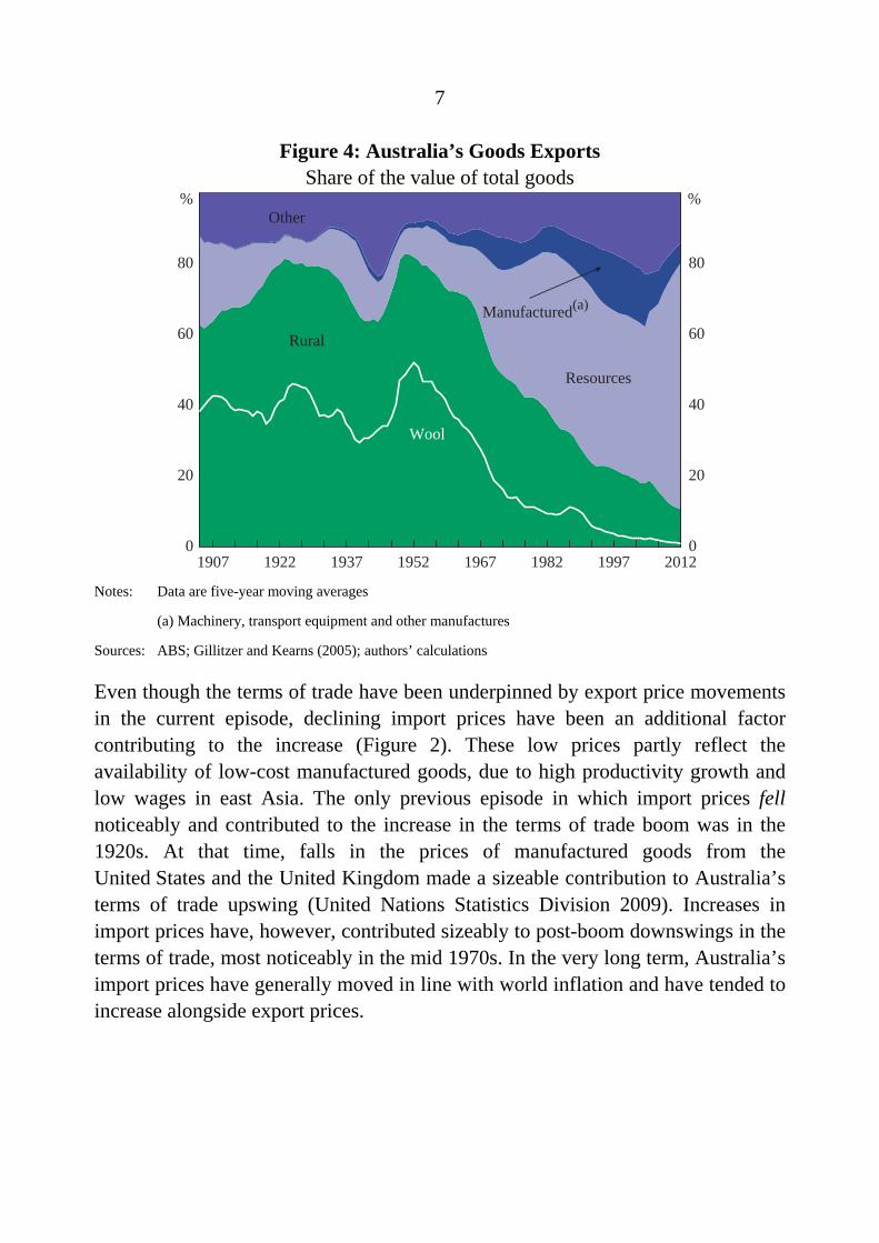
Second, export price growth was typically driven by wool and other agricultural prices, reflecting the large share of exports they accounted for at the time (Figure 3). At their peak in the early 1950s, wool exports accounted for over half of the value of Australia’s total goods exports; presently they account for less than 1 per cent (Figure 4).
Third, the prices of Australia’s natural resources have been heavily influenced by global developments and adverse supply disruptions. This has included the emergence of large countries with rapid growth prospects as well as major conflict
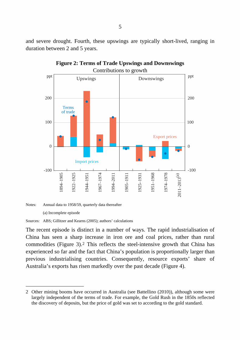
5
and severe drought. Fourth, these upswings are typically short-lived, ranging in duration between 2 and 5 years.
Figure 2: Terms of Trade Upswings and Downswings Contributions to growth
1894
–190
5
-100
0
100
200
ppt
-100
0
100
200
Downswingsppt Upswings
Termsof trade
Import prices
Export prices
1922
–192
5
1944
–195
1
1967
–197
4
1994
–201
1
1905
–191
1
1925
–193
1
1951
–196
8
1974
–197
8
2011
–201
3(a)
Notes: Annual data to 1958/59, quarterly data thereafter
(a) Incomplete episode
Sources: ABS; Gillitzer and Kearns (2005); authors’ calculations
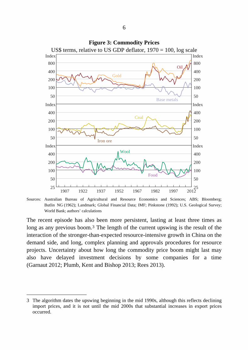
The recent episode is distinct in a number of ways. The rapid industrialisation of China has seen a sharp increase in iron ore and coal prices, rather than rural commodities (Figure 3).2 This reflects the steel-intensive growth that China has experienced so far and the fact that China’s population is proportionally larger than previous industrialising countries. Consequently, resource exports’ share of Australia’s exports has risen markedly over the past decade (Figure 4).
2 Other mining booms have occurred in Australia (see Battellino (2010)), although some were
largely independent of the terms of trade. For example, the Gold Rush in the 1850s reflected the discovery of deposits, but the price of gold was set to according to the gold standard.
6
Figure 3: Commodity Prices US$ terms, relative to US GDP deflator, 1970 = 100, log scale
Food
Index
800
400
200
100
50
25
400
200
100
50
400
200
100
50
Index
Index
Index
800
400
200
100
50
25
400
200
100
50
400
200
100
50
Index
IndexWool
Iron ore
Coal
Base metals
Oil
Gold
1907 1922 1937 1952 1967 1982 1997 2012 Sources: Australian Bureau of Agricultural and Resource Economics and Sciences; ABS; Bloomberg;
Butlin NG (1962); Landmark; Global Financial Data; IMF; Pinkstone (1992); U.S. Geological Survey;
World Bank; authors’ calculations
The recent episode has also been more persistent, lasting at least three times as long as any previous boom.3 The length of the current upswing is the result of the interaction of the stronger-than-expected resource-intensive growth in China on the demand side, and long, complex planning and approvals procedures for resource projects. Uncertainty about how long the commodity price boom might last may also have delayed investment decisions by some companies for a time (Garnaut 2012; Plumb, Kent and Bishop 2013; Rees 2013).
3 The algorithm dates the upswing beginning in the mid 1990s, although this reflects declining
import prices, and it is not until the mid 2000s that substantial increases in export prices occurred.
7
Figure 4: Australia’s Goods Exports Share of the value of total goods
1907 1922 1937 1952 1967 1982 1997 20120
20
40
60
80
0
20
40
60
80
Wool
%%
Rural
Resources
Other
Manufactured(a)
Notes: Data are five-year moving averages
(a) Machinery, transport equipment and other manufactures
Sources: ABS; Gillitzer and Kearns (2005); authors’ calculations
Even though the terms of trade have been underpinned by export price movements in the current episode, declining import prices have been an additional factor contributing to the increase (Figure 2). These low prices partly reflect the availability of low-cost manufactured goods, due to high productivity growth and low wages in east Asia. The only previous episode in which import prices fell noticeably and contributed to the increase in the terms of trade boom was in the 1920s. At that time, falls in the prices of manufactured goods from the United States and the United Kingdom made a sizeable contribution to Australia’s terms of trade upswing (United Nations Statistics Division 2009). Increases in import prices have, however, contributed sizeably to post-boom downswings in the terms of trade, most noticeably in the mid 1970s. In the very long term, Australia’s import prices have generally moved in line with world inflation and have tended to increase alongside export prices.
8
3. Macroeconomic Consequences
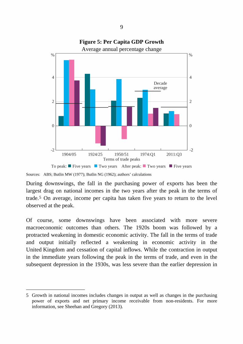
Terms of trade upswings have tended to be expansionary for the Australian economy. On average, each previous boom has coincided with per capita GDP growth that is stronger than the average over the previous decade (Figure 5).4 On the flipside, as the terms of trade fall, GDP per capita growth tends to be lower than the decadal average for two years, but returns to the average rate after five years. Consistent with stronger economic growth, the unemployment rate has tended to decline during terms of trade upswings and increase, sometimes quite sharply, during downswings in the terms of trade.
There is variation in the magnitude of output and income growth across episodes, reflecting differences in the amplitude and duration of terms of trade movements and disparate policy settings. Focusing initially on expansionary phases of terms of trade cycles, per capita output growth was particularly strong in the two years prior to the peak in the terms of trade in the early 20th century, as exports recovered after the Federation drought. However, the slow and prolonged recovery after the recession of the 1890s and the Federation drought were major headwinds to growth in the economy in the five years prior to the peak. In the early 1920s and 1950s, strong per capita output growth partly reflected pent-up demand following war and coincided with strong growth in investment.
In contrast, during the 1970s and the current episode per capita growth was below trend prior to the peak in the terms of trade. These two later episodes were affected by a disruptive negative international shock (the oil price shock and the global financial crisis). A substantial real exchange rate appreciation has occurred with nearly all upswings in the terms of trade, which is discussed further in Section 4.1.
4 Measured output growth prior to World War II is considerably more volatile than afterwards,
which may partially reflect measurement issues.
9
Figure 5: Per Capita GDP Growth Average annual percentage change
Decadeaverage
%%
To peak: Five years Two years After peak: Two years Five years
1904/05 1924/25 1950/51 1974:Q1 2011:Q3-2
0
2
4
-2
0
2
4
Terms of trade peaks
Sources: ABS; Butlin MW (1977); Butlin NG (1962); authors’ calculations
During downswings, the fall in the purchasing power of exports has been the largest drag on national incomes in the two years after the peak in the terms of trade.5 On average, income per capita has taken five years to return to the level observed at the peak.
Of course, some downswings have been associated with more severe macroeconomic outcomes than others. The 1920s boom was followed by a protracted weakening in domestic economic activity. The fall in the terms of trade and output initially reflected a weakening in economic activity in the United Kingdom and cessation of capital inflows. While the contraction in output in the immediate years following the peak in the terms of trade, and even in the subsequent depression in the 1930s, was less severe than the earlier depression in
5 Growth in national incomes includes changes in output as well as changes in the purchasing
power of exports and net primary income receivable from non-residents. For more information, see Sheehan and Gregory (2013).
10
the 1890s, the unemployment rate still reached close to 20 per cent by the early 1930s.6
The expansionary episode of the early 1970s was also followed by a downturn in global economic conditions, triggered by the global oil price shock, along with deteriorating local domestic conditions. The combination of a tightening in monetary policy in the mid 1970s, rigidities in the labour market and an overvalued nominal exchange rate contributed to per capita output growth in Australia being below average for half a decade after the peak (Pagan 1987).
The sharp slowing in real growth following the Korean War peak was short-lived. In part, this reflected strong global growth, while active fiscal and monetary policy responses to the transitory boom in wool prices also insulated the economy from the shock (Schedvin 1992; Henry 2007).
The downswing in the terms of trade in the early 20th century was an exception. GDP per capita growth remained well above its decadal average after the peak in the terms of trade. In part, this reflects the low level of average growth around that time because of the slow recovery following the severe recession of the 1890s, which involved a period of prolonged deleveraging following the collapse of the financial system. Australia’s sheep flock also took considerable time to rebuild after the Federation drought; the export boom in wool only got underway in the early 20th century.7 The fall in the terms of trade was also relatively mild, with prices remaining at high levels, as there was no major global downturn.
While the consequences of terms of trade cycles for the major expenditure components of GDP will be discussed in more detail in the following subsections, the key points are:
6 Between 1891 and 1895, real GDP declined by almost 20 per cent. The 1890s depression was
exacerbated by several idiosyncratic factors, including a banking crisis associated with the collapse of a property price bubble in Melbourne (see Simon (2003) and Kent (2011)). Maddock and McLean (1987) also suggest that structural imbalances in the local economy and high external indebtedness exacerbated the downturn in the 1890s.
7 Public investment also made a noticeable contribution to growth (Maddock and McLean 1987).
11
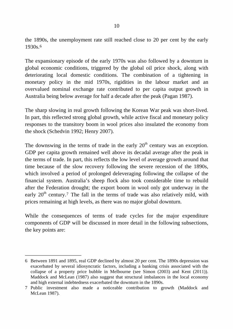
Investment contributed strongly to GDP per capita growth before peaks in the terms of trade, with the exception of the early 1900s (Figure 6). Increased investment reflects the business sector seeking to increase supply in response to higher commodity prices. Dwelling investment also generally contributes to growth during these periods, with the exception of the early 1900s and the most recent cycle.
Net exports weighed on growth leading up to the peaks in the terms of trade, although there were considerable differences across episodes. Export volume growth took time to respond to higher prices in many cases and the accompanying real exchange rate appreciation weighed on the rest of the tradeables sector (see Section 4.1). Following peaks in the terms of trade, net exports contributed to GDP growth, notably in the 1950s and 1970s episodes, and the real exchange rate depreciated.
Figure 6: Contributions to GDP per Capita Growth Before (B) and after (A) terms of trade peaks
B A B A B A B A B A-9
-6
-3
0
3
6
9
-9
-6
-3
0
3
6
9
Terms of trade peaks
ppt1904/05(a) 1924/25 1950/51 1974:Q1 2011:Q3
GDP percapita
Private consumption Public demand Private investment Inventories Net exports
ppt
Notes: Average annual contribution five years before and two years after terms of trade peaks
(a) Before peak based on data between 1900/01 and 1904/05
Sources: ABS; Butlin MW (1977); authors’ calculations
12
3.1 Investment
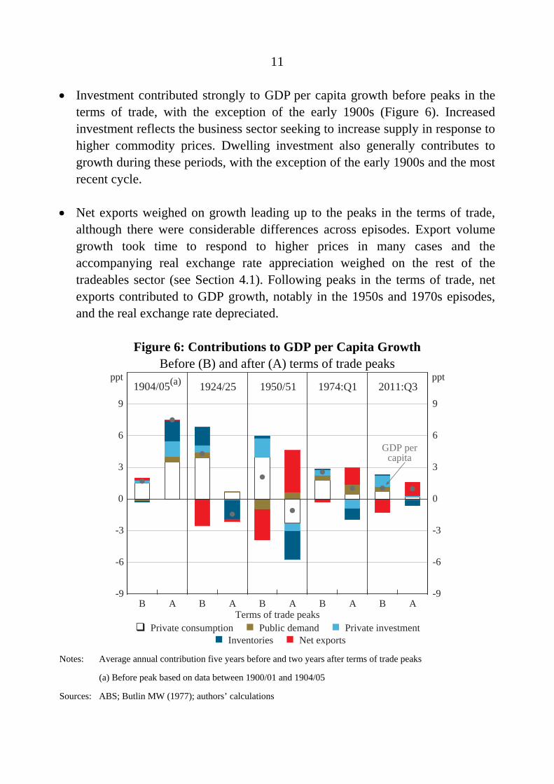
Major upswings in the terms of trade have reflected increases in commodity prices accompanying strong global growth, resulting in higher marginal returns to investment in the resources and rural sectors. As such, terms of trade booms are generally accompanied by strong investment growth in these and other parts of the economy (Figure 7). Dwelling and business investment grew quickly during most upswings and made substantial contributions to output per capita growth. Increased investment in public infrastructure also typically contributed to growth during terms of trade upswings. Very high investment has also been a key characteristic of the current episode. Much of this has been driven by investment in the resources sector, which has reached a historically high 8 per cent of GDP.8
Figure 7: Private Investment per Capita
1904
/05
1924
/25
1950
/51
1974
:Q1
2011
:Q3-10
0
10
20
30
40Before peak
%
1904
/05
1924
/25
1950
/51
1974
:Q1
2011
:Q3 -10
0
10
20
30
40
Business investment%
Dwelling investment
After peak
Terms of trade peaks Note: Average annual growth five years before and two years after terms of trade peaks
Sources: ABS; Butlin MW (1977); authors’ calculations
8 The accumulation of livestock for wool (but not food), is treated in the national accounts as
investment. The relationship between the terms of trade and the livestock investment series is not strong, probably reflecting measurement issues and supply disturbances (such as drought).
13
Differences in the characteristics of resources, rural and other forms of investment have important consequences for the size and duration of the investment response. In particular, some forms of investment can take long periods before becoming productive. The planning and approval processes associated with resources investment are more extensive than many other forms of investment. These time-to-build characteristics of resources investment lead to a long supply lag that keeps commodity prices higher than they otherwise would be.
A large movement in the terms of trade, and a concomitant change in the real exchange rate, can also affect investment at a sectoral level, as it discourages investment in the other tradeable sectors. However, to the extent that the real appreciation is in part owing to a nominal exchange rate appreciation, it also makes imported capital goods cheaper.
Private dwelling investment did not contribute sizably to output per capita growth in the current cycle as the terms of trade rose. Indeed, the cyclicality of dwelling investment evident historically has been largely absent since the early 2000s; it is an open question why this has occurred. One possibility is that supply-side issues in the housing market have meant that increased household incomes have flown more so into higher house prices. Also, income gains coming via the corporate sector in the current episode probably have been muted by foreign ownership of the mining sector (see Connolly and Orsmond (2011)).
Growth in overall investment has tended to moderate as the terms of trade decline. However, a notable exception was the early 20th century episode, when the rate of growth of investment was higher than in the upswing phase. This situation reflected the fact that private investment picked up following the period of weakness and deleveraging associated with the 1890s depression and the end of the Federation drought.
3.2 Trade
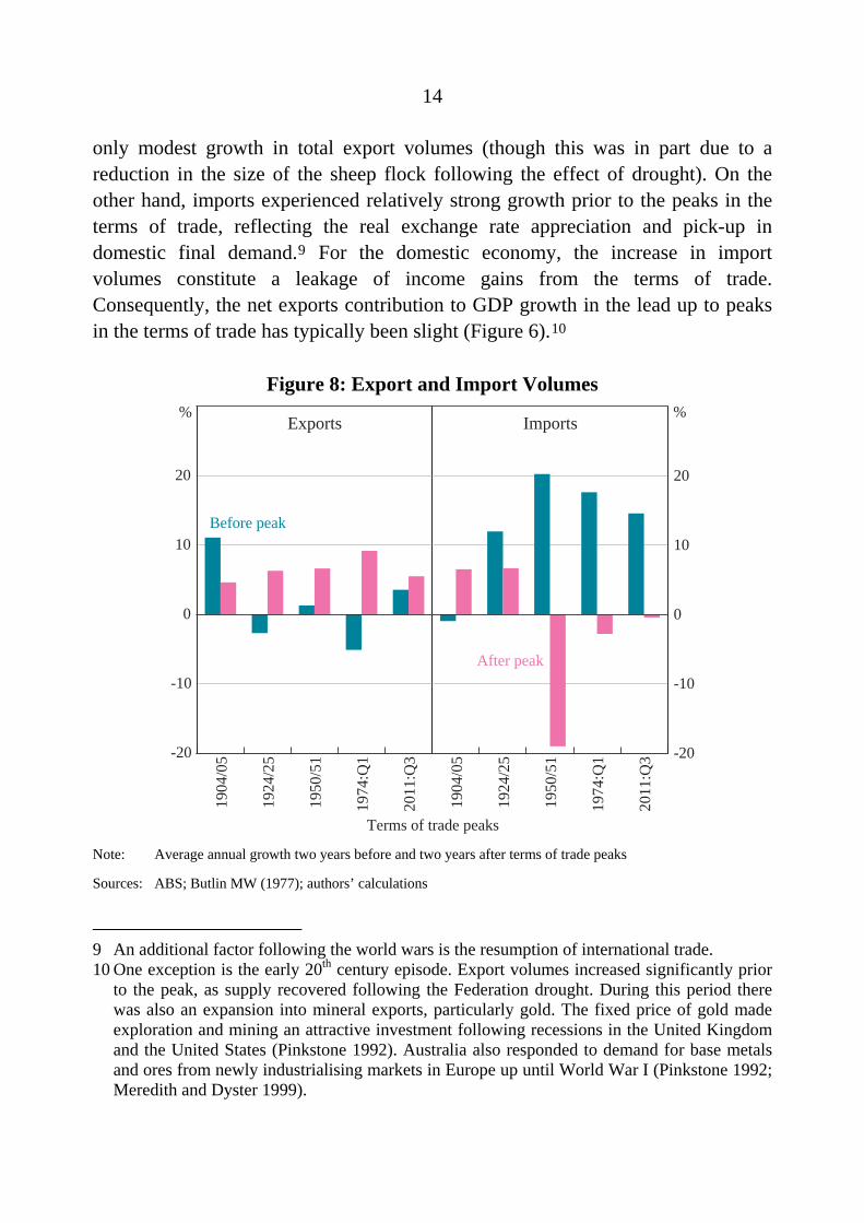
Export volumes have generally experienced weak growth in the period preceding a terms of trade peak (Figure 8). In part, this reflects the accompanying rise in the real exchange rate and the sluggishness with which commodity production can respond to higher prices. For example, during the Korean War boom there was
14
only modest growth in total export volumes (though this was in part due to a reduction in the size of the sheep flock following the effect of drought). On the other hand, imports experienced relatively strong growth prior to the peaks in the terms of trade, reflecting the real exchange rate appreciation and pick-up in domestic final demand.9 For the domestic economy, the increase in import volumes constitute a leakage of income gains from the terms of trade. Consequently, the net exports contribution to GDP growth in the lead up to peaks in the terms of trade has typically been slight (Figure 6).10
Figure 8: Export and Import Volumes
1904
/05
1924
/25
1950
/51
1974
:Q1
2011
:Q3-20
-10
0
10
20
%
1904
/05
1924
/25
1950
/51
1974
:Q1
2011
:Q3 -20
-10
0
10
20
Before peak
%
After peak
Exports Imports
Terms of trade peaks Note: Average annual growth two years before and two years after terms of trade peaks
Sources: ABS; Butlin MW (1977); authors’ calculations
9 An additional factor following the world wars is the resumption of international trade. 10 One exception is the early 20th century episode. Export volumes increased significantly prior
to the peak, as supply recovered following the Federation drought. During this period there was also an expansion into mineral exports, particularly gold. The fixed price of gold made exploration and mining an attractive investment following recessions in the United Kingdom and the United States (Pinkstone 1992). Australia also responded to demand for base metals and ores from newly industrialising markets in Europe up until World War I (Pinkstone 1992; Meredith and Dyster 1999).
15
In the most recent episode, growth in resource export volumes was also subdued following the initial pick-up in commodity prices. This is likely to have reflected uncertainty about the longevity of the higher prices together with the time it takes for resources investment to become productive. As a result, average growth in total export volumes in the first decade of the 21st century was the lowest since World War II, although this reflected weak performance in a number of resource exports, as well as across rural commodities, manufactures and services (Plumb et al 2013). The sizeable real exchange rate appreciation that accompanied the increase in the terms of trade also restrained export growth outside of the resources sector; downturns in trading partner growth in the early 2000s and the global financial crisis were also factors.
Following peaks in the terms of trade, exports growth typically increased in the short term as supply came on line and the real exchange rate declined. A slowdown in imports growth has also typically followed peaks in the terms of trade.11
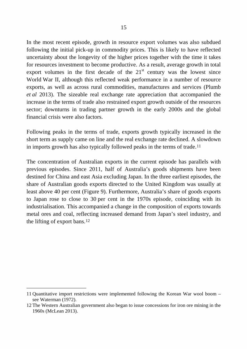
The concentration of Australian exports in the current episode has parallels with previous episodes. Since 2011, half of Australia’s goods shipments have been destined for China and east Asia excluding Japan. In the three earliest episodes, the share of Australian goods exports directed to the United Kingdom was usually at least above 40 per cent (Figure 9). Furthermore, Australia’s share of goods exports to Japan rose to close to 30 per cent in the 1970s episode, coinciding with its industrialisation. This accompanied a change in the composition of exports towards metal ores and coal, reflecting increased demand from Japan’s steel industry, and the lifting of export bans.12
11 Quantitative import restrictions were implemented following the Korean War wool boom –
see Waterman (1972). 12 The Western Australian government also began to issue concessions for iron ore mining in the
1960s (McLean 2013).
16
Figure 9: Export Destinations Share of total, five-year centred moving average
1905 1920 1935 1950 1965 1980 1995 20100
15
30
45
0
15
30
45
UK
%%
Japan
East Asia(a)
China
Notes: Goods exports; financial years; shaded regions denote expansionary phases for Australia’s terms of trade
(a) Excludes China and Japan; data prior to 1952/53 are not available
Sources: ABS; Pinkstone (1992); Vamplew (1987); authors’ calculations
3.3 Consumption
A change in the terms of trade may influence per capita consumption in several ways. First, it may alter the composition of the consumption bundle by changing the relative price of imports to domestically produced goods. This could occur as a result of a change in the nominal exchange rate. Increases in low-cost manufacturing in the 1920s and the current episode have also suppressed world, and hence Australian import, prices. Second, a change in the terms of trade also affects income, although the extent to which this influences consumption depends on whether the movements are perceived as permanent or temporary.
The behaviour of consumption per capita growth differs considerably across episodes (Figure 10). Growth was particularly strong during the Roaring Twenties, coinciding with lower unemployment and higher asset prices and wealth. In the lead up to the peak in the terms of trade in the 1950s, consumption growth was weak relative to its high decadal average. The effects of a ‘wartime economy’, such as production shortages and rationing controls, difficulties obtaining imported
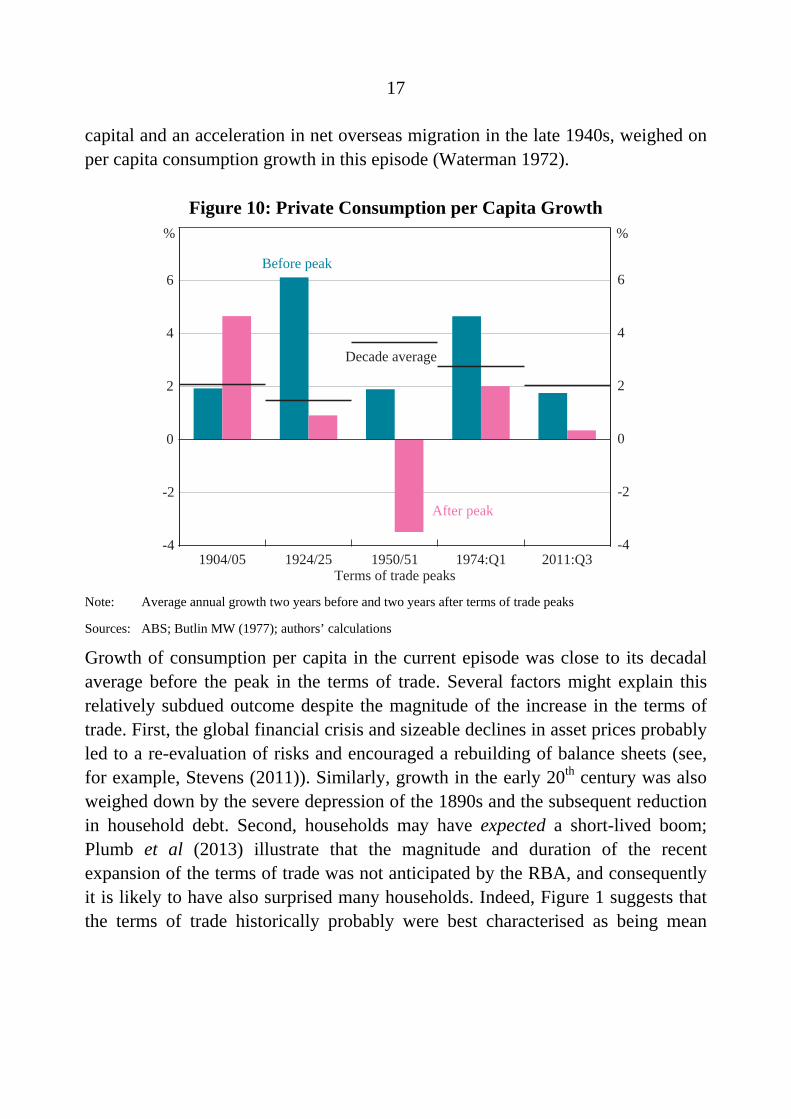
17
capital and an acceleration in net overseas migration in the late 1940s, weighed on per capita consumption growth in this episode (Waterman 1972).
Figure 10: Private Consumption per Capita Growth
1904/05 1924/25 1950/51 1974:Q1 2011:Q3-4
-2
0
2
4
6
-4
-2
0
2
4
6
Terms of trade peaks
Before peak
%
After peak
Decade average
%
Note: Average annual growth two years before and two years after terms of trade peaks
Sources: ABS; Butlin MW (1977); authors’ calculations
Growth of consumption per capita in the current episode was close to its decadal average before the peak in the terms of trade. Several factors might explain this relatively subdued outcome despite the magnitude of the increase in the terms of trade. First, the global financial crisis and sizeable declines in asset prices probably led to a re-evaluation of risks and encouraged a rebuilding of balance sheets (see, for example, Stevens (2011)). Similarly, growth in the early 20th century was also weighed down by the severe depression of the 1890s and the subsequent reduction in household debt. Second, households may have expected a short-lived boom; Plumb et al (2013) illustrate that the magnitude and duration of the recent expansion of the terms of trade was not anticipated by the RBA, and consequently it is likely to have also surprised many households. Indeed, Figure 1 suggests that the terms of trade historically probably were best characterised as being mean

18
reverting.13 A high degree of foreign ownership of the resources sector may have been another factor.
A further possibility is that some households might have been credit constrained, and thus unable to bring forward their consumption in anticipation of higher future incomes, although the financial deregulation of the 1980s has removed these constraints relative to the past.
4. Economic Policy Settings and Terms of Trade Episodes
This section contrasts past policies and their effects with those in the current episode. Historically, macroeconomic policy frameworks were more rigid and not well equipped to handle shocks. In some cases this led to economic outcomes that were highly disruptive. Today’s policy frameworks and institutional structures allow greater flexibility within the economy. While not all parts of the economy have directly benefited, these policies have assisted in producing a relatively smooth adjustment process in a macroeconomic sense relative to past booms. These settings and frameworks may help facilitate the necessary macroeconomic adjustments as the terms of trade declines.
4.1 Monetary Policy
Monetary policy in Australia has operated under various frameworks during the past 150 years. These have included fixed exchange rate regimes, money supply targets and inflation targeting under a floating exchange rate. Each framework has sought, with varying degrees of success, to limit monetary expansion and contain inflation (Cornish 2010).
Policy in earlier episodes was constrained by the fixed or pegged exchange rate regime. This was supported by the use of instruments such as capital controls and qualitative and quantitative controls on credit. In addition, the prevailing wisdom among policymakers in the 1960s and 1970s was that full employment was the primary goal, with less emphasis on inflationary consequences, limiting the scope for the central bank to respond to inflationary pressures stemming from terms of
13 Unit root tests on data over the entire sample suggest the Australian terms of trade are
stationary, whereas data from 1955 onwards appear to be non-stationary.
19
trade booms. There was also little communication with the public regarding monetary policy initiatives (Cagliarini, Kent and Stevens 2010).
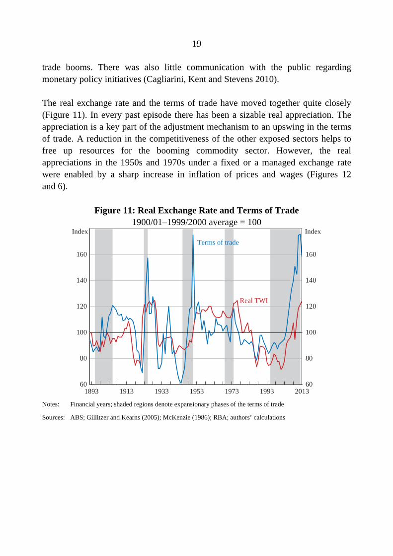
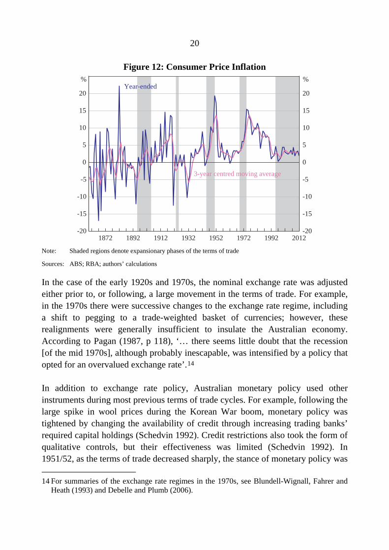
The real exchange rate and the terms of trade have moved together quite closely (Figure 11). In every past episode there has been a sizable real appreciation. The appreciation is a key part of the adjustment mechanism to an upswing in the terms of trade. A reduction in the competitiveness of the other exposed sectors helps to free up resources for the booming commodity sector. However, the real appreciations in the 1950s and 1970s under a fixed or a managed exchange rate were enabled by a sharp increase in inflation of prices and wages (Figures 12 and 6).
Figure 11: Real Exchange Rate and Terms of Trade 1900/01–1999/2000 average = 100
1893 1913 1933 1953 1973 1993 201360
80
100
120
140
160
60
80
100
120
140
160
Terms of trade
IndexIndex
Real TWI
Notes: Financial years; shaded regions denote expansionary phases of the terms of trade
Sources: ABS; Gillitzer and Kearns (2005); McKenzie (1986); RBA; authors’ calculations
20
Figure 12: Consumer Price Inflation
Year-ended% %
3-year centred moving average
1872 1892 1912 1932 1952 1972 1992 2012-20
-15
-10
-5
0
5
10
15
20
-20
-15
-10
-5
0
5
10
15
20
Note: Shaded regions denote expansionary phases of the terms of trade
Sources: ABS; RBA; authors’ calculations
In the case of the early 1920s and 1970s, the nominal exchange rate was adjusted either prior to, or following, a large movement in the terms of trade. For example, in the 1970s there were successive changes to the exchange rate regime, including a shift to pegging to a trade-weighted basket of currencies; however, these realignments were generally insufficient to insulate the Australian economy. According to Pagan (1987, p 118), ‘… there seems little doubt that the recession [of the mid 1970s], although probably inescapable, was intensified by a policy that opted for an overvalued exchange rate’.14
In addition to exchange rate policy, Australian monetary policy used other instruments during most previous terms of trade cycles. For example, following the large spike in wool prices during the Korean War boom, monetary policy was tightened by changing the availability of credit through increasing trading banks’ required capital holdings (Schedvin 1992). Credit restrictions also took the form of qualitative controls, but their effectiveness was limited (Schedvin 1992). In 1951/52, as the terms of trade decreased sharply, the stance of monetary policy was
14 For summaries of the exchange rate regimes in the 1970s, see Blundell-Wignall, Fahrer and
Heath (1993) and Debelle and Plumb (2006).
21
relaxed, primarily through central bank loans and the release of ‘special account’ holdings to trading banks (Schedvin 1992).
The rise and subsequent fall in the terms of trade in the 1970s coincided with large fluctuations in net capital inflows, stagflation, political instability and the collapse of the Bretton Woods system of fixed exchange rates, all of which posed difficulties for monetary policy.15 In the early 1970s, the RBA had difficulty managing the increased capital inflows and capital controls were used.16 Meanwhile, the banking sector was still highly regulated and the RBA continued to use both qualitative and quantitative controls.17
Prior to the current terms of trade cycle, the RBA adopted an inflation-targeting framework, with the goal of keeping consumer inflation between 2 and 3 per cent on average over the medium term. This framework has provided a clear nominal anchor which, together with changes to the structure of the labour market described in Section 4.5, limited the feedback of the boom to economy-wide prices and wages. Notwithstanding the very significant rise in the terms of trade in the current episode, inflation has been well contained, especially when compared to the experience of the 1950s or 1970s. The floating exchange rate and inflation-targeting framework has also provided the RBA with the flexibility to maintain an accommodative stance of monetary policy more recently to support domestic demand since the terms of trade has started to fall.
15 Schedvin (1992) characterised the degree of difficulty in conducting monetary policy in the
1970s to that in the 1960s as a ‘quantum leap’. 16 The capital controls included an embargo on short-term capital inflows and a Variable
Deposit Requirement, which required a fraction of overseas borrowings to be deposited at the RBA in an interest-free account, effectively serving as a tax (Treasury 1999).
17 For example, a policy statement from the RBA’s 1969-70 annual report (RBA 1970, p 48): ‘It was announced that, in the course of its contacts with savings banks, trading banks, and life offices, the Bank had asked these institutions to maintain, and in the case of savings banks, to the extent practicable to increase, the volume of their housing loans in coming months. This action followed the recent falling-off in dwelling approvals by local government authorities and indications of a decline in housing commencements’. See also Battellino and McMillan (1989).
22
4.2 Fiscal Policy
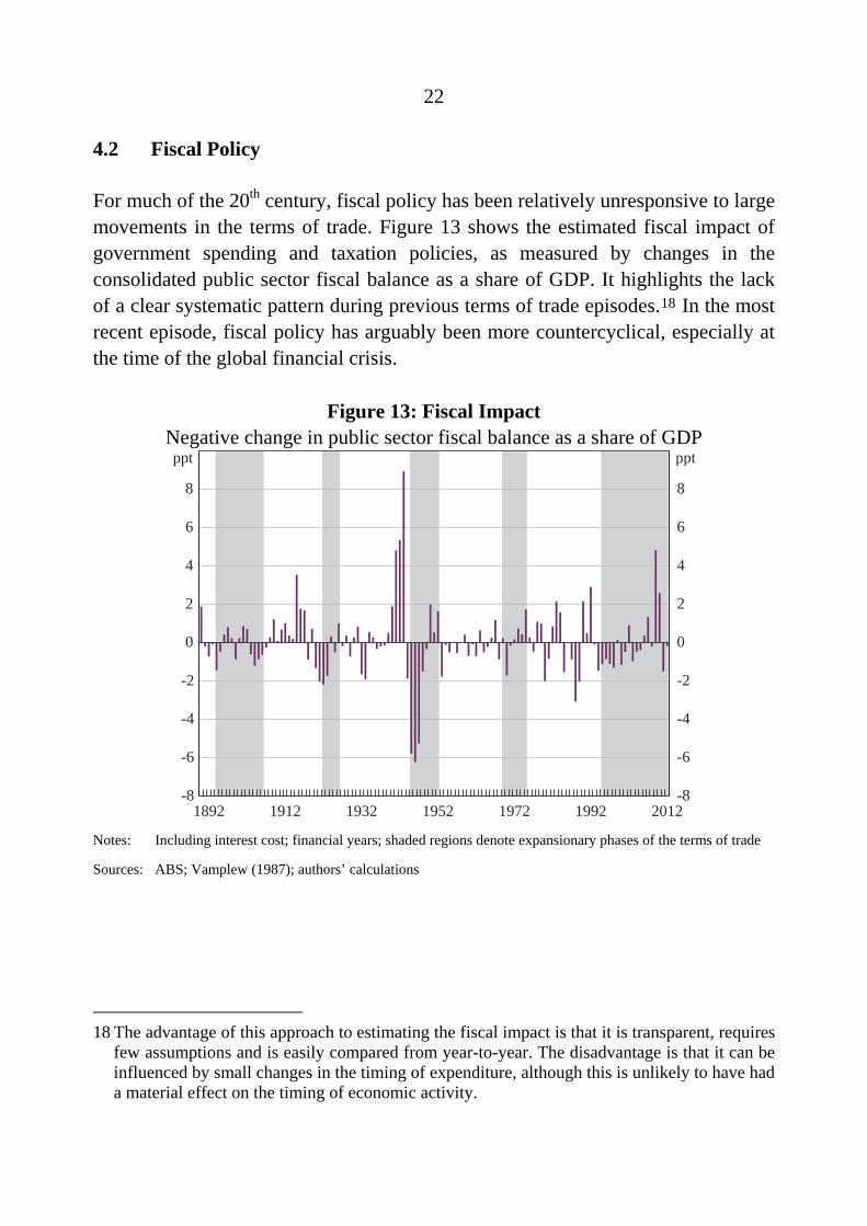
For much of the 20th century, fiscal policy has been relatively unresponsive to large movements in the terms of trade. Figure 13 shows the estimated fiscal impact of government spending and taxation policies, as measured by changes in the consolidated public sector fiscal balance as a share of GDP. It highlights the lack of a clear systematic pattern during previous terms of trade episodes.18 In the most recent episode, fiscal policy has arguably been more countercyclical, especially at the time of the global financial crisis.
Figure 13: Fiscal Impact Negative change in public sector fiscal balance as a share of GDP
ppt
1892 1912 1932 1952 1972 1992 2012-8
-6
-4
-2
0
2
4
6
8
-8
-6
-4
-2
0
2
4
6
8
ppt
Notes: Including interest cost; financial years; shaded regions denote expansionary phases of the terms of trade
Sources: ABS; Vamplew (1987); authors’ calculations
18 The advantage of this approach to estimating the fiscal impact is that it is transparent, requires
few assumptions and is easily compared from year-to-year. The disadvantage is that it can be influenced by small changes in the timing of expenditure, although this is unlikely to have had a material effect on the timing of economic activity.
23
Australia’s fiscal position in the first half of the 20th century partly reflected a strong desire among policymakers to operate a balanced budget.19 Outside periods of war, Australia’s consolidated revenue fund (CRF) – the fiscal position net of all expenditures and receipts except those to and from loan accounts – remained broadly in balance through the Federation, Roaring Twenties and Korean War wool booms. Indeed, during the Great Depression, governments at the Premiers’ Conference declared their determination to balance their respective budgets for 1930/31, and to maintain this stance in future years (Australia, House of Representatives 1930).
Public revenue and expenditure have both become larger as a share of the economy over time. Australia’s tax take increased from around 5 per cent of GDP at the turn of the 20th century to more than 20 per cent currently. There was a shift towards income taxation away from indirect taxes, particularly following the uniform income taxation legislation of 1942 (Pincus 1987). Indirect taxes have declined from constituting virtually all federal revenue during the terms of trade boom around Federation to now be less than 20 per cent of the total.20 Alongside the expansion in the tax base, personal and company income tax rates have declined and are lower than in previous episodes such as in the 1950s and the 1970s (Reinhardt and Steel 2006). Overall, these changes have had a significant effect on the fiscal position in the current episode, including increasing the sensitivity and cyclicality of revenue collections to fluctuations in economic activity and the terms of trade and lifting incentives for workforce participation and investment.
Over the 40 years after Federation, the use of indirect taxes was favoured partly for reasons of feasibility (Reinhardt and Steel 2006). As a consequence, the automatic responsiveness of tax collections to fluctuations in macroeconomic conditions was relatively minor in a number of earlier terms of trade episodes (Pincus 1988). During the Korean War wool boom the efficacy of revaluing the currency or using a tax on income from wool exports was actively discussed.21 The Government
19 Achieving a balanced budget was considered to be ‘the hallmark of good government’
(Australia, House of Representatives 1959). 20 In 1901, customs and receipts from public enterprises accounted for nearly all Commonwealth
revenue (Vamplew 1987). 21 A revaluation was opposed by exporters of agricultural products other than wool, while
graziers denounced the tax on wool incomes as a ‘class tax’ (Waterman 1972).
24
responded in 1950/51 by imposing a levy and mandatory savings of receipts from wool sales (Waterman 1972).
Government expenditure was also relatively small as a share of GDP in the very early terms of trade episodes, limiting the ability to stimulate the economy. During the Federation and the Roaring Twenties episodes, there was a consensus among economists and policymakers that public expenditure only had a limited role in stabilising economic cycles (Garnaut 2005).22 In the current episode, however, the larger size of the government ensures some buffer to activity via automatic stabilisers to the downturn in the terms of trade, and the attitude among some economists to a discretionary fiscal policy response has changed, particularly for spending on infrastructure (see, for example, Garnaut (2013) and Sheehan and Gregory (2013)).
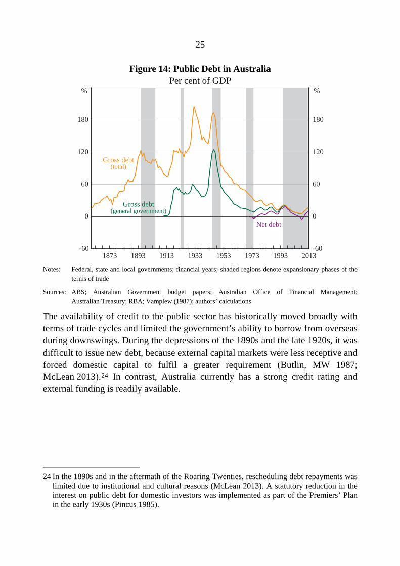
The level of public debt has been much higher in historical cycles and this also constrained the government’s ability to respond to weaker economic conditions with sizeable discretionary fiscal stimulus. Figure 14 shows that total gross public debt was well above 100 per cent of nominal GDP during Federation and up to the Korean War, while in the 1970s it remained above 50 per cent of nominal GDP. The primary reason for the large size of public debt in the past was the legacy of major conflict and the ‘settler nature’ of the Australian economy, the latter requiring high rates of social and economic infrastructure. In contrast, public debt in the current episode is at low levels.23
22 The so-called ‘horror’ budget of 1951 explicitly recognised for the first time in Australian
history that the budget should be used for countercyclical policy purposes (Waterman 1972). Most of the initiatives were focused on the revenue side and included increases in income, sales and company tax (Schedvin 1970).
23 Government gross debt is the total liability the government owes to creditors. This is comprised largely of outstanding Commonwealth Government securities. Net debt is gross debt less the debt owed to the government. For a summary of the historical trends of public debt in Australia, see Di Marco, Pirie and Au-Yeung (2009).
25
Figure 14: Public Debt in Australia Per cent of GDP
1873 1893 1913 1933 1953 1973 1993 2013-60
0
60
120
180
-60
0
60
120
180
Gross debt(total)
% %
Gross debt(general government)
Net debt
Notes: Federal, state and local governments; financial years; shaded regions denote expansionary phases of the
terms of trade
Sources: ABS; Australian Government budget papers; Australian Office of Financial Management;
Australian Treasury; RBA; Vamplew (1987); authors’ calculations
The availability of credit to the public sector has historically moved broadly with terms of trade cycles and limited the government’s ability to borrow from overseas during downswings. During the depressions of the 1890s and the late 1920s, it was difficult to issue new debt, because external capital markets were less receptive and forced domestic capital to fulfil a greater requirement (Butlin, MW 1987; McLean 2013).24 In contrast, Australia currently has a strong credit rating and external funding is readily available.
24 In the 1890s and in the aftermath of the Roaring Twenties, rescheduling debt repayments was
limited due to institutional and cultural reasons (McLean 2013). A statutory reduction in the interest on public debt for domestic investors was implemented as part of the Premiers’ Plan in the early 1930s (Pincus 1985).

26
4.3 Population Policy
Large-scale immigration has been an enduring feature of Australian history. Booms in the terms of trade have generally coincided with strong growth in net overseas migration (Figure 15). The cyclical pattern partly reflects economic conditions and relative job opportunities. That some terms of trade upswings have occurred following major conflict means that geopolitical issues such as displaced workers after World War II have also contributed. In contrast, downswings have coincided with a slowing in growth in migration and increasing unemployment.
Figure 15: Net Overseas Migration Per cent of resident population
1873 1893 1913 1933 1953 1973 1993 2013-3
-2
-1
0
1
2
3
-3
-2
-1
0
1
2
3
%%
Note: Shaded regions denote expansionary phases of the terms of trade
Sources: ABS; authors’ calculations
Migration policy has been used as a form of stabilisation policy during previous cycles (Butlin, Barnard and Pincus 1982). Immigration was used to meet skill shortages, affect demand for non-tradeables and to foster growth in trade-exposed and import-competing industries (such as manufacturing and agriculture). For example, skilled immigration was encouraged in the 1920s, which was important in the textiles and iron & steel industries (Pope 1987). In the 1950s, foreign migrant workers participated extensively in public works, while in the 1960s and
27
early 1970s they were a key input into trade-exposed manufacturing and non-tradeable industries such as construction (Meredith and Dyster 1999).
4.4 Trade Protection
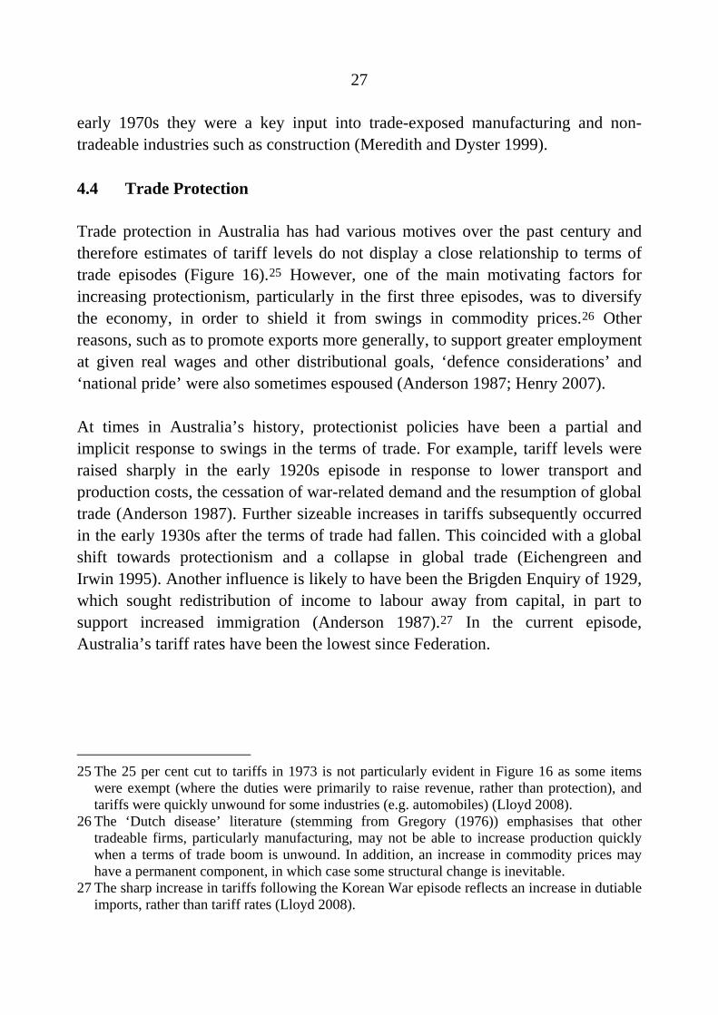
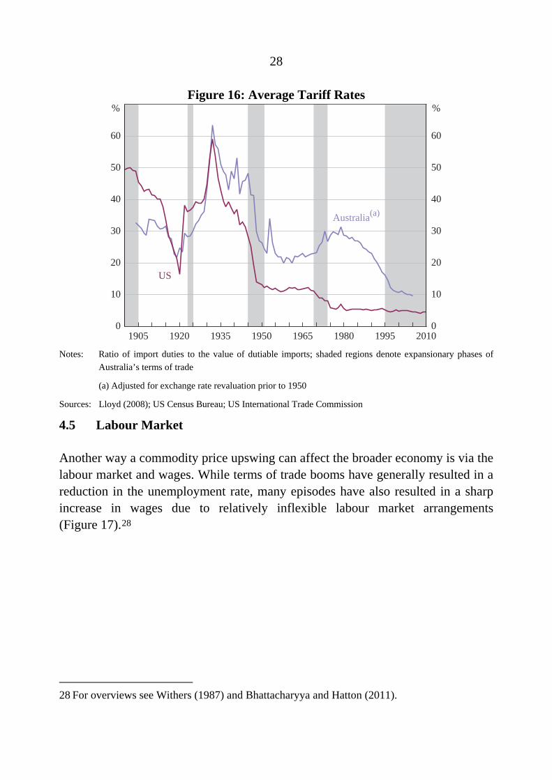
Trade protection in Australia has had various motives over the past century and therefore estimates of tariff levels do not display a close relationship to terms of trade episodes (Figure 16).25 However, one of the main motivating factors for increasing protectionism, particularly in the first three episodes, was to diversify the economy, in order to shield it from swings in commodity prices.26 Other reasons, such as to promote exports more generally, to support greater employment at given real wages and other distributional goals, ‘defence considerations’ and ‘national pride’ were also sometimes espoused (Anderson 1987; Henry 2007).
At times in Australia’s history, protectionist policies have been a partial and implicit response to swings in the terms of trade. For example, tariff levels were raised sharply in the early 1920s episode in response to lower transport and production costs, the cessation of war-related demand and the resumption of global trade (Anderson 1987). Further sizeable increases in tariffs subsequently occurred in the early 1930s after the terms of trade had fallen. This coincided with a global shift towards protectionism and a collapse in global trade (Eichengreen and Irwin 1995). Another influence is likely to have been the Brigden Enquiry of 1929, which sought redistribution of income to labour away from capital, in part to support increased immigration (Anderson 1987).27 In the current episode, Australia’s tariff rates have been the lowest since Federation.
25 The 25 per cent cut to tariffs in 1973 is not particularly evident in Figure 16 as some items
were exempt (where the duties were primarily to raise revenue, rather than protection), and tariffs were quickly unwound for some industries (e.g. automobiles) (Lloyd 2008).
26 The ‘Dutch disease’ literature (stemming from Gregory (1976)) emphasises that other tradeable firms, particularly manufacturing, may not be able to increase production quickly when a terms of trade boom is unwound. In addition, an increase in commodity prices may have a permanent component, in which case some structural change is inevitable.
27 The sharp increase in tariffs following the Korean War episode reflects an increase in dutiable imports, rather than tariff rates (Lloyd 2008).
28
Figure 16: Average Tariff Rates
1905 1920 1935 1950 1965 1980 1995 20100
10
20
30
40
50
60
0
10
20
30
40
50
60
Australia(a)
%%
US
Notes: Ratio of import duties to the value of dutiable imports; shaded regions denote expansionary phases of
Australia’s terms of trade
(a) Adjusted for exchange rate revaluation prior to 1950
Sources: Lloyd (2008); US Census Bureau; US International Trade Commission
4.5 Labour Market
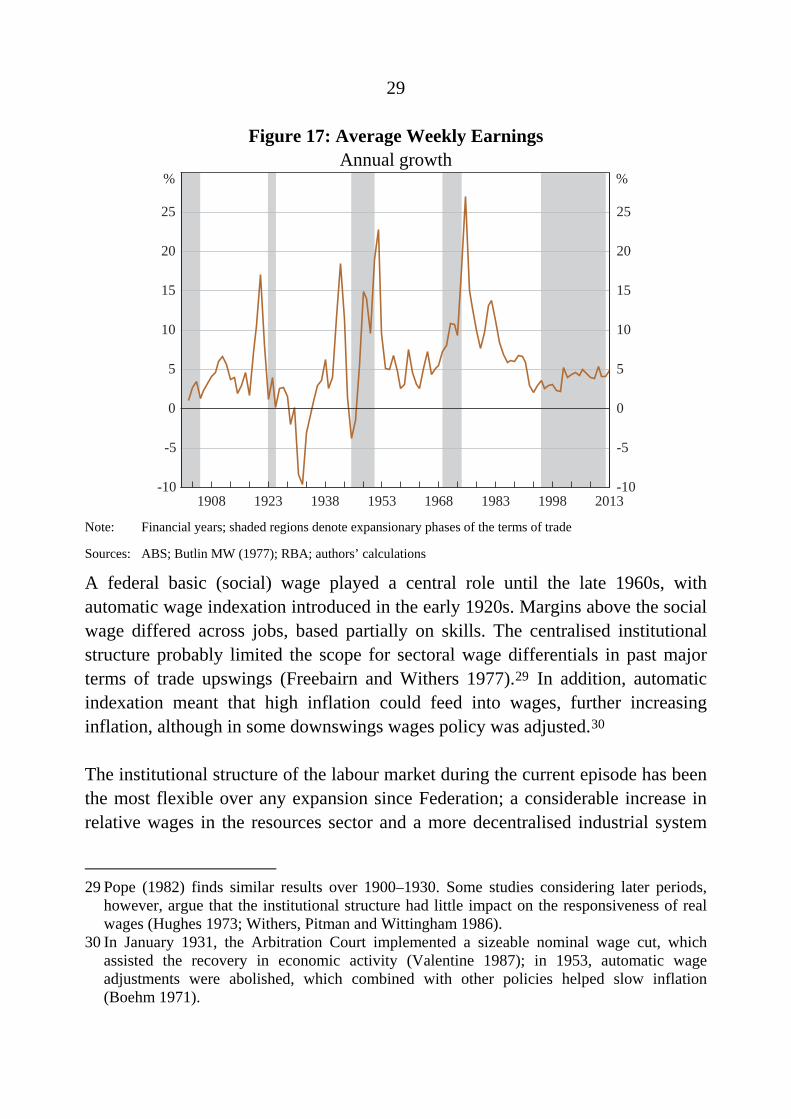
Another way a commodity price upswing can affect the broader economy is via the labour market and wages. While terms of trade booms have generally resulted in a reduction in the unemployment rate, many episodes have also resulted in a sharp increase in wages due to relatively inflexible labour market arrangements (Figure 17).28
28 For overviews see Withers (1987) and Bhattacharyya and Hatton (2011).
29
Figure 17: Average Weekly Earnings Annual growth
1908 1923 1938 1953 1968 1983 1998 2013-10
-5
0
5
10
15
20
25
-10
-5
0
5
10
15
20
25
% %
Note: Financial years; shaded regions denote expansionary phases of the terms of trade
Sources: ABS; Butlin MW (1977); RBA; authors’ calculations
A federal basic (social) wage played a central role until the late 1960s, with automatic wage indexation introduced in the early 1920s. Margins above the social wage differed across jobs, based partially on skills. The centralised institutional structure probably limited the scope for sectoral wage differentials in past major terms of trade upswings (Freebairn and Withers 1977).29 In addition, automatic indexation meant that high inflation could feed into wages, further increasing inflation, although in some downswings wages policy was adjusted.30
The institutional structure of the labour market during the current episode has been the most flexible over any expansion since Federation; a considerable increase in relative wages in the resources sector and a more decentralised industrial system
29 Pope (1982) finds similar results over 1900–1930. Some studies considering later periods,
however, argue that the institutional structure had little impact on the responsiveness of real wages (Hughes 1973; Withers, Pitman and Wittingham 1986).
30 In January 1931, the Arbitration Court implemented a sizeable nominal wage cut, which assisted the recovery in economic activity (Valentine 1987); in 1953, automatic wage adjustments were abolished, which combined with other policies helped slow inflation (Boehm 1971).
30
facilitated a relatively low unemployment rate during the upswing in the terms of trade without creating substantial inflationary pressures.
The dynamics of labour demand in the current episode are also considerably different to those of the past because the phases in a mining boom are more distinct than in an agricultural-based boom (see, for example, Corden and Neary (1982) and Plumb et al (2013)). In particular, in the construction phase, when capacity is expanded, there is both strong investment and demand for labour. However, once the expansion in capacity is complete and mines are operational, it is likely that labour needs will be relatively less.31
The responsiveness of labour supply to a booming sector depends on factors such as the extent of specialised skills required and its geographic location. D’Arcy et al (2012) reported that as at February 2012 nearly one-fifth of employed people had begun their job in the previous year, suggesting that there was considerable labour mobility. They also note that around half of all job movements at this time involved job changes between industries. Alternatively, some studies have found the responsiveness of labour to intra-industry wage differentials to be limited (e.g. Kilpatrick and Felmingham (1996a, 1996b), using data from 1989 and 1992). D’Arcy et al (2012) argue that in the current episode the non-financial costs of relocating and skills mismatch have to some extent restricted geographic mobility; Bhattacharyya and Williamson (2011) examine differences in unemployment rates across the states, and find that since the 1920s boom labour has been geographically immobile.32
5. Conclusions
Australia’s current terms of trade cycle has parallels with earlier episodes. Historically, large movements in the terms of trade were mainly driven by changes in export prices, particularly wool, which reflected strong demand from
31 In both types of boom, however, there may be considerable increases in employment in
industries servicing the booming sector (for example, the business services or construction sectors).
32 Watson (2011) (using Household Income and Labour Dynamics in Australia (HILDA) data) found that in both 2002 and 2008 only 6 per cent of people changing jobs moved 500 kilometres or more. Debelle and Vickery (1999) also found little role for wage differentials in influencing interstate labour mobility.

31
industrialising economies, coupled with adverse supply developments, such as drought. Upswings in the terms of trade have generally boosted domestic demand, usually with a sizeable contribution from investment, probably reflecting both a direct response to higher commodity prices and the associated improvement in wealth and confidence. In some episodes, growth in immigration and pent-up demand following war also supported growth in investment. Typically, net exports have contributed little to economic growth during the upswing in the terms of trade; sluggish supply responses are exacerbated by the real exchange rate appreciation, which dampens growth in other exports and supports imports. Many of these features have been present in the current episode.
The current episode, however, has some distinct features. One is that it has been mostly related to bulk commodities, instead of rural commodities. Consequently, the sluggish response of supply partly reflects the characteristics of resources investment – namely long periods to plan and gain approval for projects and the need to develop infrastructure. However, just as Australia was the world’s major source for internationally traded wool throughout previous episodes, today it is the world’s largest exporter of steel-making materials and it is likely that Australia will also become a major source of liquefied natural gas exports in the coming years. A decline in the terms of trade is therefore, to some extent, the result of new supply from Australian producers coming on-line.
The most recent upswing was the largest sustained increase of the terms of trade on record, and the Australian economy is likely to continue to be a beneficiary of strong growth in Asia. Indications suggest China’s industrialisation and urbanisation process, which has underpinned the increase in demand for steel-making commodities, is likely to continue for a number of years, although it may well grow more slowly than in the past. Chinese infrastructure needs remain large; an example is that steel demand for residential construction is not estimated to peak until around 2024 (Berkelmans and Wang 2012). While the path of economic development is not always smooth, it is important to remember that this is not the first episode during which one country and a narrow range of commodities have been of particular importance to the Australian economy; rather, that is the norm.
32
Another stark difference is that despite the unprecedented movement in the terms of trade, the macroeconomic adjustments in Australia have been relatively smooth. Inflation, for example, has remained contained, in contrast to many previous experiences, such as the Korean War wool boom. Furthermore, inflation expectations have remained relatively low and stable. Factors facilitating this include the greater flexibility present in the labour market, the inflation-targeting regime adopted by the RBA, and the flexible nominal exchange rate, which has enabled the necessary appreciation of the real exchange rate to occur in a less disruptive manner.
Historically, for several years following a peak in the terms of trade, growth in investment and output per capita tends to be below average. As we have emphasised, the real exchange rate and the terms of trade generally move together. Consequently, the expected easing in the terms of trade, reflecting growth in the global supply of the bulk commodities, may be accompanied by falls in the real exchange rate. More generally, an increase in Australia’s competitiveness would help facilitate the macroeconomic adjustments necessary during the transition from the investment to production phase by providing support to sectors outside of the resources sector, thereby helping to rebalance growth in the economy. Reflecting the unparalleled magnitude of the expansion, the transition necessary is considerable and is likely to pose challenges to both firms and policymakers. The current policy frameworks and institutional structures, which were important in facilitating better macroeconomic outcomes during the upswing than occurred historically, may also assist this transition.
33
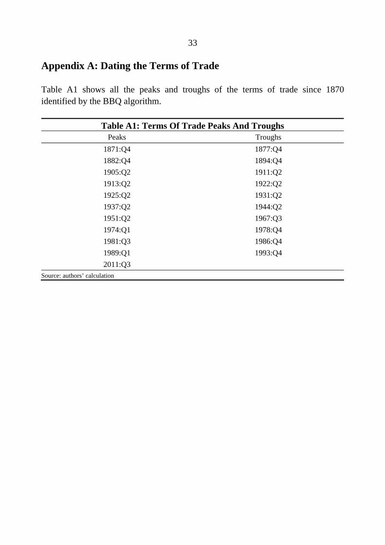
Appendix A: Dating the Terms of Trade
Table A1 shows all the peaks and troughs of the terms of trade since 1870 identified by the BBQ algorithm.
Table A1: Terms Of Trade Peaks And Troughs Peaks Troughs
1871:Q4 1877:Q4
1882:Q4 1894:Q4
1905:Q2 1911:Q2
1913:Q2 1922:Q2
1925:Q2 1931:Q2
1937:Q2 1944:Q2
1951:Q2 1967:Q3
1974:Q1 1978:Q4
1981:Q3 1986:Q4
1989:Q1 1993:Q4
2011:Q3
Source: authors’ calculation
34
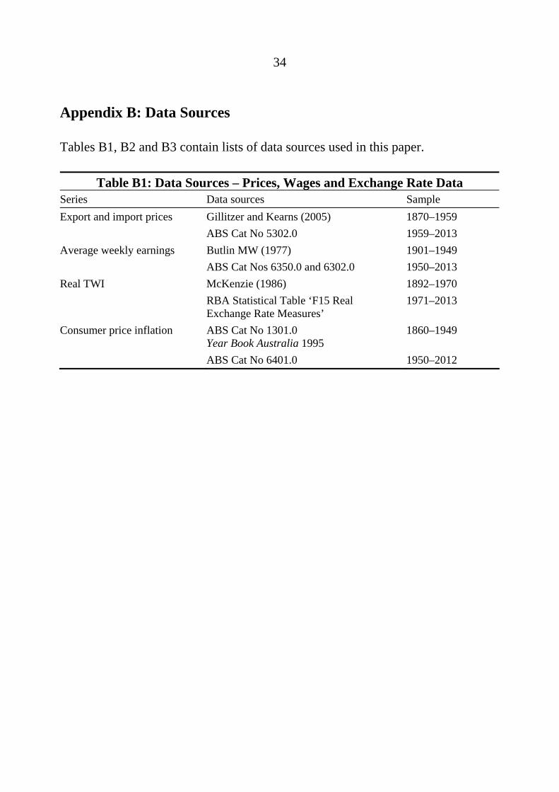
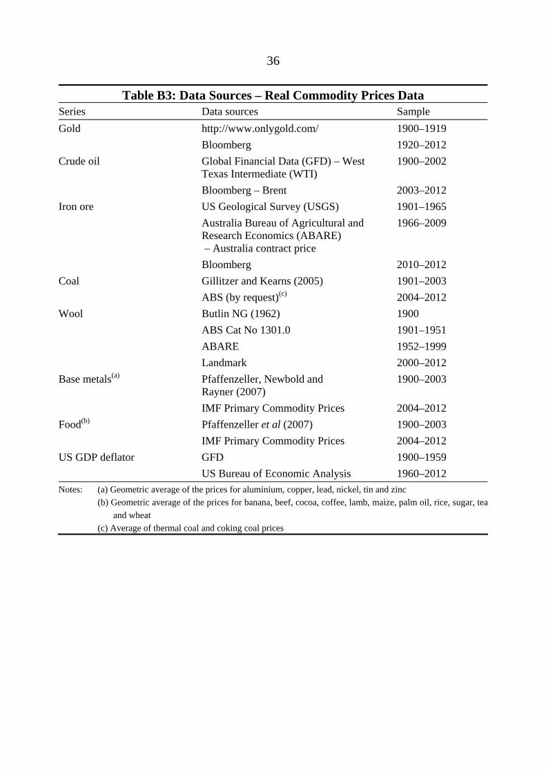
Appendix B: Data Sources
Tables B1, B2 and B3 contain lists of data sources used in this paper.
Table B1: Data Sources – Prices, Wages and Exchange Rate Data Series Data sources Sample
Export and import prices Gillitzer and Kearns (2005) 1870–1959
ABS Cat No 5302.0 1959–2013
Average weekly earnings Butlin MW (1977) 1901–1949
ABS Cat Nos 6350.0 and 6302.0 1950–2013
Real TWI McKenzie (1986) 1892–1970
RBA Statistical Table ‘F15 Real Exchange Rate Measures’
1971–2013
Consumer price inflation ABS Cat No 1301.0 Year Book Australia 1995
1860–1949
ABS Cat No 6401.0 1950–2012
35
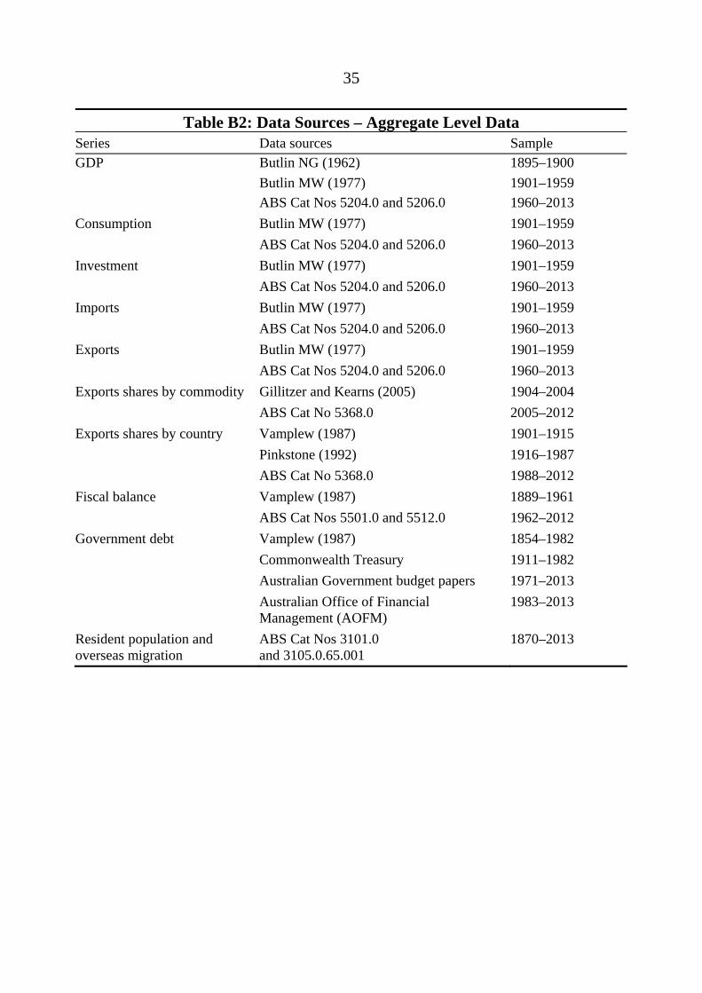
Table B2: Data Sources – Aggregate Level Data Series Data sources Sample GDP Butlin NG (1962) 1895–1900 Butlin MW (1977) 1901–1959 ABS Cat Nos 5204.0 and 5206.0 1960–2013
Consumption Butlin MW (1977) 1901–1959
ABS Cat Nos 5204.0 and 5206.0 1960–2013
Investment Butlin MW (1977) 1901–1959
ABS Cat Nos 5204.0 and 5206.0 1960–2013
Imports Butlin MW (1977) 1901–1959
ABS Cat Nos 5204.0 and 5206.0 1960–2013
Exports Butlin MW (1977) 1901–1959
ABS Cat Nos 5204.0 and 5206.0 1960–2013
Exports shares by commodity Gillitzer and Kearns (2005) 1904–2004
ABS Cat No 5368.0 2005–2012
Exports shares by country Vamplew (1987) 1901–1915
Pinkstone (1992) 1916–1987
ABS Cat No 5368.0 1988–2012
Fiscal balance Vamplew (1987) 1889–1961
ABS Cat Nos 5501.0 and 5512.0 1962–2012
Government debt Vamplew (1987) 1854–1982
Commonwealth Treasury 1911–1982
Australian Government budget papers 1971–2013
Australian Office of Financial Management (AOFM)
1983–2013
Resident population and overseas migration
ABS Cat Nos 3101.0 and 3105.0.65.001
1870–2013
36
Table B3: Data Sources – Real Commodity Prices Data Series Data sources Sample
Gold http://www.onlygold.com/ 1900–1919
Bloomberg 1920–2012
Crude oil Global Financial Data (GFD) – West Texas Intermediate (WTI)
1900–2002
Bloomberg – Brent 2003–2012
Iron ore US Geological Survey (USGS) 1901–1965
Australia Bureau of Agricultural and Research Economics (ABARE) – Australia contract price
1966–2009
Bloomberg 2010–2012
Coal Gillitzer and Kearns (2005) 1901–2003
ABS (by request)(c) 2004–2012
Wool Butlin NG (1962) 1900
ABS Cat No 1301.0 1901–1951
ABARE 1952–1999
Landmark 2000–2012
Base metals(a) Pfaffenzeller, Newbold and Rayner (2007)
1900–2003
IMF Primary Commodity Prices 2004–2012
Food(b) Pfaffenzeller et al (2007) 1900–2003
IMF Primary Commodity Prices 2004–2012
US GDP deflator GFD 1900–1959
US Bureau of Economic Analysis 1960–2012
Notes: (a) Geometric average of the prices for aluminium, copper, lead, nickel, tin and zinc
(b) Geometric average of the prices for banana, beef, cocoa, coffee, lamb, maize, palm oil, rice, sugar, tea
and wheat
(c) Average of thermal coal and coking coal prices
37
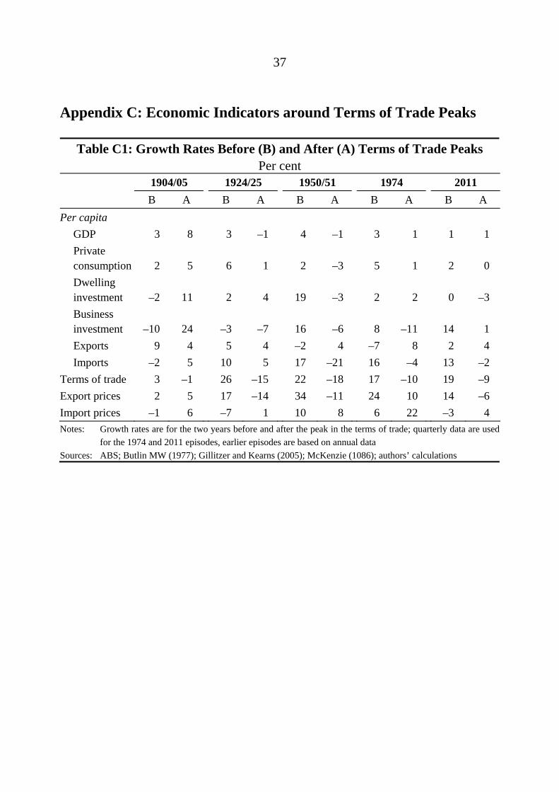
Appendix C: Economic Indicators around Terms of Trade Peaks
Table C1: Growth Rates Before (B) and After (A) Terms of Trade Peaks Per cent
1904/05 1924/25 1950/51 1974 2011
B A B A B A B A B A
Per capita
GDP 3 8 3 –1 4 –1 3 1 1 1
Private consumption 2 5 6 1 2 –3 5 1 2 0
Dwelling investment –2 11 2 4 19 –3 2 2 0 –3
Business investment –10 24 –3 –7 16 –6 8 –11 14 1
Exports 9 4 5 4 –2 4 –7 8 2 4
Imports –2 5 10 5 17 –21 16 –4 13 –2
Terms of trade 3 –1 26 –15 22 –18 17 –10 19 –9
Export prices 2 5 17 –14 34 –11 24 10 14 –6
Import prices –1 6 –7 1 10 8 6 22 –3 4
Notes: Growth rates are for the two years before and after the peak in the terms of trade; quarterly data are used
for the 1974 and 2011 episodes, earlier episodes are based on annual data
Sources: ABS; Butlin MW (1977); Gillitzer and Kearns (2005); McKenzie (1086); authors’ calculations
38
References
Anderson K (1987), ‘Tariffs and the Manufacturing Sector’, in R Maddock and IW McLean (eds), The Australian Economy in the Long Run, Cambridge University Press, Cambridge, pp 165–194.
Australia, House of Representatives (1930), Debates, vol HR47, pp 533–539. Fragment available at: <http://parlinfo.aph.gov.au/parlInfo/genpdf/hansard80/ hansardr80/1930-11-20/0118/hansard_frag.pdf;fileType=application%2Fpdf>.
Australia, House of Representatives (1959), Debates, vol HR35, pp 577–579. Fragment available at: <http://parlinfo.aph.gov.au/parlInfo/genpdf/hansard80/ hansardr80/1959-08-26/0117/hansard_frag.pdf;fileType=application%2Fpdf>.
Battellino R (2010), ‘Mining Booms and the Australian Economy’, RBA Bulletin, March, pp 63–69.
Battellino R and N McMillan (1989), ‘Changes in the Behaviour of Banks and Their Implications for Financial Aggregates’, RBA Research Discussion Paper No 8904.
Berkelmans L and H Wang (2012), ‘Chinese Urban Residential Construction to 2040’, RBA Research Discussion Paper No 2012-04.
Bhattacharyya S and TJ Hatton (2011), ‘Australian Unemployment in the Long Run, 1903–2007’, The Economic Record, 87(277), pp 202–220.
Bhattacharyya S and JG Williamson (2011), ‘Commodity Price Shocks and the Australian Economy since Federation’, Australian Economic History Review, 51(2), pp 150–177.
Blundell-Wignall A, J Fahrer and A Heath (1993), ‘Major Influences on the Australian Dollar Exchange Rate’, in A Blundell-Wignall (ed), The Exchange Rate, International Trade and the Balance of Payments, Proceedings of a Conference, Reserve Bank of Australia, Sydney, pp 30–78.
39
Boehm EA (1971), Twentieth Century Economic Development in Australia, Topics on the Australian Economy, Longman Australia Pty Limited, Camberwell.
Butlin MW (1977), ‘A Preliminary Annual Database 1900/01 to 1973/74’, RBA Research Discussion Paper No 7701.
Butlin MW (1987), ‘Capital Markets’, in R Maddock and IW McLean (eds), The Australian Economy in the Long Run, Cambridge University Press, Cambridge, pp 229–247.
Butlin NG (1962), Australian Domestic Product, Investment and Foreign Borrowing, 1861–1938/39, Cambridge University Press, Cambridge.
Butlin NG, A Barnard and JJ Pincus (1982), Government and Capitalism: Public and Private Choice in Twentieth Century Australia, George Allen & Unwin, Sydney.
Cagliarini A, C Kent and G Stevens (2010), ‘Fifty Years of Monetary Policy: What Have We Learned?’, in C Kent and M Robson (eds), Reserve Bank of Australia 50th Anniversary Symposium, Proceedings of a Conference, Reserve Bank of Australia, Sydney, pp 9–37.
Connolly E and D Orsmond (2011), ‘The Mining Industry: From Bust to Boom’, RBA Research Discussion Paper No 2011–08.
Cooper RN and RZ Lawrence (1975), ‘The 1972–75 Commodity Boom’, Brookings Papers on Economic Activity, 1975(3), pp 671–715.
Corden WM and JP Neary (1982), ‘Booming Sector and De-Industrialisation in a Small Open Economy’, The Economic Journal, 92(368), pp 825–848.
Cornish S (2010), The Evolution of Central Banking in Australia, Reserve Bank of Australia, Sydney.
D’Arcy P, L Gustafsson, C Lewis and T Wiltshire (2012), ‘Labour Market Turnover and Mobility’, RBA Bulletin, December, pp 1–12.
40
Debelle G and M Plumb (2006), ‘The Evolution of Exchange Rate Policy and Capital Controls in Australia’, Asian Economic Papers, 5(2), pp 7–29.
Debelle G and J Vickery (1999), ‘Labour Market Adjustment: Evidence on Interstate Labour Mobility’, The Australian Economic Review, 32(3), pp 249–263.
Di Marco K, M Pirie and W Au-Yeung (2009), ‘A History of Public Debt in Australia’, Economic Roundup, Issue 1, pp 1–15.
Eichengreen B and DA Irwin (1995), ‘Trade Blocs, Currency Blocs and the Reorientation of World Trade in the 1930s’, Journal of International Economics, 38(1–2), pp 1–24.
Freebairn J and G Withers (1977), ‘The Performance of Manpower Forecasting Techniques in Australian Labour Markets’, Australian Bulletin of Labour, 4(1), pp 13–31.
Garnaut R (2005), ‘Is Macroeconomics Dead? Monetary and Fiscal Policy in Historical Context’, Oxford Review of Economic Policy, 21(4), pp 524–531.
Garnaut R (2012), ‘The Contemporary China Resources Boom’, The Australian Journal of Agricultural and Resource Economics, 56(2), pp 222–243.
Garnaut R (2013), Dog Days: Australia after the Boom, Redback, Collingwood.
Gillitzer C and J Kearns (2005), ‘Long-Term Patterns in Australia’s Terms of Trade’, RBA Research Discussion Paper No 2005-01.
Gregory RG (1976), ‘Some Implications of the Growth in the Mineral Sector’, The Australian Journal of Agricultural Economics, 20(2), pp 71–91.
Gruen D (2006), ‘A Tale of Two Terms-Of-Trade Booms’, Economic Roundup, Summer, pp 21–34.
Harding D and A Pagan (2002), ‘Dissecting the Cycle: A Methodological Investigation’, Journal of Monetary Economics, 49(2), pp 365–381.
41
Henry K (2007), ‘Achieving and Maintaining Full Employment’, The 2007 Sir Roland Wilson Foundation Lecture, Sir Roland Wilson Foundation, Canberra, 14 August.
Hughes B (1973), ‘The Wages of the Strong and the Weak’, Journal of Industrial Relations, 15(1), pp 1–20.
Kent C (2011), ‘Two Depressions, One Banking Collapse: Lessons From Australia’, Journal of Financial Stability, 7(3), pp 126–137.
Kilpatrick S and B Felmingham (1996a), ‘Labour Mobility in Australian Industry’, Applied Economics Letters, 3(9), pp 577–579.
Kilpatrick S and B Felmingham (1996b), ‘Labour Mobility in the Australian Regions’, The Economic Record, 72(218), pp 214–223.
Lloyd P (2008), ‘100 Years of Tariff Protection in Australia’, Australian Economic History Review, 48(2), pp 99–145.
Maddock R and IW McLean (1987), ‘The Australian Economy in the Very Long Run’, in R Maddock and IW McLean (eds), The Australian Economy in the Long Run, Cambridge University Press, Cambridge, pp 5–29.
McKenzie IM (1986), ‘Australia’s Real Exchange Rate during the Twentieth Century’, The Economic Record, Supplement, pp 69–78.
McLean IW (2013), Why Australia Prospered: The Shifting Sources of Economic Growth, Princeton University Press, Princeton.
Meredith D and B Dyster (1999), Australia in the Global Economy: Continuity and Change, Cambridge University Press, Cambridge.
Pagan A (1987), ‘The End of The Long Boom’, in R Maddock and IW McLean (eds), The Australian Economy in the Long Run, Cambridge University Press, Cambridge, pp 106–130.
42
Pfaffenzeller S, P Newbold and A Rayner (2007), ‘A Short Note on Updating the Grilli and Yang Commodity Price Index’, The World Bank Economic Review, 21(1), pp 151–163.
Pincus JJ (1985), ‘Aspects of Australian Public Finances and Public Enterprises, 1920 to 1939’, Paper presented at the Conference on the Recovery from the Depression in Australia 1931–1937, convened by the Department of Economic History and Centre for Economic Policy Research, Australian National University, Canberra,12–14 August.
Pincus JJ (1987), ‘Government’, in R Maddock and IW McLean (eds), The Australian Economy in the Long Run, Cambridge University Press, Cambridge, pp 291–318.
Pincus JJ (1988), ‘Australian Budgetary Policies in the 1930s’, in RG Gregory and NG Butlin (eds), Recovery from the Depression: Australia and the World Economy in the 1930s, Cambridge University Press, Melbourne, pp 173–192.
Pinkstone B with the collaboration of D Meredith (1992), Global Connections: A History of Exports and the Australian Economy, Australian Government Publishing Service, Canberra.
Plumb M, C Kent and J Bishop (2013), ‘Implications for the Australian Economy of Strong Growth in Asia’, RBA Research Discussion Paper No 2013-03.
Pope D (1982), ‘Wage Regulation and Unemployment in Australia, 1900-30’, Australian Economic History Review, 22(2), pp 103–126.
Pope D (1987), ‘Population and Australian Economic Development 1900–1930’, in R Maddock and IW McLean (eds), The Australian Economy in the Long Run, Cambridge University Press, Cambridge, pp 33–60.
Rees D (2013), ‘Terms of Trade Shocks and Incomplete Information’, RBA Research Discussion Paper No 2013-09.
43
Reinhardt S and L Steel (2006), ‘A Brief History of Australia’s Tax System’, Economic Roundup, Winter, pp 1–26.
RBA (Reserve Bank of Australia) (1970), Report and Financial Statements, Reserve Bank of Australia, Sydney.
Schedvin CB (1970), Australia and the Great Depression: A Study of Economic Development and Policy in the 1920s and 1930s, Sydney University Press, Sydney.
Schedvin CB (1992), In Reserve: Central Banking in Australia, 1945-75, Allen and Unwin Pty Ltd, St Leonards.
Sheehan P and RG Gregory (2013), ‘The Resources Boom and Economic Policy in the Long Run’, The Australian Economic Review, 46(2), pp 121–139.
Simon J (2003), ‘Three Australian Asset-Price Bubbles’, in A Richards and T Robinson (eds), Asset Prices and Monetary Policy, Proceedings of a Conference, Reserve Bank of Australia, Sydney, pp 8–41.
Smith B (1987), ‘The Role of Resource Development in Australia’s Economic Growth’, Australian National University, Centre for Economic Policy Research Discussion Paper No 167.
Stevens G (2011), ‘The Cautious Consumer’, Address to the Anika Foundation Luncheon supported by Australian Business Economists and Macquarie Bank, Sydney, 26 July.
Treasury (Commonwealth Treasury of Australia) (1999), ‘Australia’s Experience with the Variable Deposit Requirement’, Economic Roundup, Winter, pp 45–56.
United Nations Statistics Division (2009), ‘Historical Data 1900-1960 on International Merchandise Trade Statistics’, accessed on 11 October 2013. Available at <http://unstats.un.org/unsd/trade/imts/historical_data.htm>.
44
Valentine T (1987), ‘The Depression of the 1930s’, in R Maddock and IW McLean (eds), The Australian Economy in the Long Run, Cambridge University Press, Cambridge, pp 61–78.
Vamplew W (ed) (1987), Australians: Historical Statistics, Australians: A Historical Library, Volume 10, Fairfax, Syme & Weldon Associates, Sydney.
Waterman AMC (1972), Economic Fluctuations in Australia, 1948 to 1964, Australian National University Press, Canberra.
Watson I (2011), ‘Does Changing Your Job Leave You Better Off? A Study of Labour Mobility in Australia, 2002 to 2008’, National Centre for Vocational Education Research (NCVER) Occasional Paper, April.
Withers G (1987), ‘Labour’, in R Maddock and IW McLean (eds), The Australian Economy in the Long Run, Cambridge University Press, Cambridge, pp 248–288.
Withers G, D Pitman and B Whittingham (1986), ‘Wage Adjustments and Labour Market Systems: A Cross-Country Analysis’, The Economic Record, 62(179), pp 415–426.
RESEARCH DISCUSSION PAPERS
These papers can be downloaded from the Bank’s website or a hard copy may be obtained by writing to:
Mail Room Supervisor Information Department Reserve Bank of Australia GPO Box 3947 SYDNEY NSW 2001
Enquiries:
Phone: +61 2 9551 9830 Facsimile: +61 2 9551 8033 Email: [email protected] Website: http://www.rba.gov.au
2013-05 Liquidity Shocks and the US Housing Credit Crisis of Gianni La Cava 2007–2008
2013-06 Estimating and Identifying Empirical BVAR-DSGE Models Tim Robinson for Small Open Economies
2013-07 An Empirical BVAR-DSGE Model of the Australian Economy Sean Langcake Tim Robinson
2013-08 International Business Cycles with Complete Markets Alexandre Dmitriev Ivan Roberts
2013-09 Terms of Trade Shocks and Incomplete Information Daniel Rees
2013-10 Stochastic Terms of Trade Volatility in Small Open Economies Patricia Gómez-González Daniel Rees
2013-11 Issues in Estimating New-Keynesian Phillips Curves in the Mariano Kulish Presence of Unknown Structural Change Adrian Pagan
2013-12 Central Counterparty Links and Clearing System Exposures Nathanael Cox Nicholas Garvin Gerard Kelly
2013-13 Inventory Investment in Australia and the Global Financial Gianni La Cava Crisis
2013-14 Reserves of Natural Resources in a Small Open Economy Isaac Gross James Hansen
2013-15 Trends in Funding and Lending Behaviour of Australian Banks Chris Stewart Benn Robertson Alexandra Heath