The “Fiscal Cliff”: Macroeconomic Consequences of Tax ... · The “Fiscal Cliff”: Macroeconomic Consequences of Tax Increases and Spending Cuts Congressional Research Service

CRS Report for CongressPrepared for Members and Committees of Congress

The “Fiscal Cliff”: Macroeconomic Consequences of Tax Increases and Spending Cuts

Jane G. Gravelle Senior Specialist in Economic Policy

January 9, 2013

Congressional Research Service

7-5700 www.crs.gov

R42700



Summary A major policy concern for Congress has been when and whether to address the “fiscal cliff,” a set of tax increases and spending cuts that would have substantially reduced the deficit in 2013. In projections made in March 2012 by the Congressional Budget Office (CBO), this fiscal restraint, constituting 5.1% of output in 2013, would have reduced growth to 0.5% from 4.4%. Unemployment would increase by 2 million. In August, updated estimates projected growth at a negative 0.5%. The American Taxpayer Relief Act (H.R. 8) eliminated part of the fiscal cliff.

Policy choices with respect to the fiscal cliff are difficult because of the conflict between short-run and long-run economic and budgetary objectives. In the short run, the reduction in demand from the reduced budget deficits could damage an already fragile recovery. In the longer run, however, deficit reduction is needed to address a projected unsustainable debt level.

For FY2013, compared with FY2012, the original policy-related fiscal cliff was projected at $502 billion, 80% reflecting tax increases, with an additional $105 billion from other changes. The expiration of the 2001, 2003, and 2009 tax cuts (extended in 2010) and the expiration of the alternative minimum tax (AMT) “patch,” which indexes the AMT exemption for inflation, accounted for 44% of the policy-related fiscal cliff. Other tax provisions included expiration of the temporary two percentage-point reduction in the employee’s Social Security payroll tax (19%); the expiration of other tax cuts, including depreciation and the “extenders” (13%); and taxes scheduled to come into effect as a part of health reform (4%). Spending reductions included the automatic spending cuts under the Budget Control Act (13%); the expiration of extended unemployment insurance benefits (5%); and the “doc fix” that would have lowered Medicare payments (2%). Most changes would have taken effect after 2012, although the AMT and many of the extenders expired after 2011.

CBO estimates were similar to those of other forecasters. Estimates are uncertain; CBO suggested a range of potential reductions in growth from 0.9% to 6.8% if the fiscal cliff occurred. Thus, the effects could have been much smaller, but they could also have been significantly larger, than CBO’s mid-point estimate. Different parts of the cliff were projected to have different effects per dollar of budgetary effects, with larger effects from the automatic budget cuts and ending extended unemployment benefits than from ending tax cuts for higher-income individuals.

H.R. 8 passed by the House on January 1, 2013 (after previous Senate approval) eliminated two-thirds of the policy-related fiscal cliff, and slightly over half of the total (including non-policy-related provisions). Thus about half of the contractionary effect remains, which would appear to reduce output by about 2%. H.R. 8 permanently extended the 2001 and 2003 income tax cuts, except for high-income taxpayers and the $5 million exemption for the estate taxes (but with a higher rate). It extended the 2009 cuts through 2017. It extended unemployment insurance benefits, the doc fix, and bonus depreciation and the “extenders” through 2013. It delayed the automatic spending cuts for two months. Elements of the fiscal cliff that will continue to reduce the deficit in 2013 compared with 2012, and potentially exert a contractionary effect, are the payroll tax reduction, which expired; some individual income tax cuts for high-income individuals; tax increases enacted in health reform; the remaining budget cuts; and non-policy-related effects.



Contents Introduction ...................................................................................................................................... 1 The Size and Composition of the Original Fiscal Cliff ................................................................... 2 Revisions in H.R. 8 .......................................................................................................................... 7 Aggregate Short-Run Effects of the Original Fiscal Cliff ............................................................... 9 Differential Effects of the Components of the Fiscal Cliff ............................................................ 10 Effect on the Economy of the Fiscal Cliff as Altered by H.R. 8 .................................................... 15 Implications for Policy Choices ..................................................................................................... 16

Tables Table 1. CBO Estimates of the Original Fiscal Cliff—Reductions in the Budget Deficit in

FY2013 Compared with FY2012 ................................................................................................. 4 Table 2. Increases in the Deficit Due to Changing the Fiscal Cliff, FY2013 and FY2014 .............. 6 Table 3. Tax Revenue Losses and Spending Increases in H.R. 8 ..................................................... 8 Table 4. Multipliers for Components of the American Recovery and Investment Act of

2009 (ARRA; P.L. 111-5) for the First Quarter of 2012 ............................................................. 12 Table 5. Multiplier Effect of Selected Stimulus Policies, 2012-2013 ............................................ 12 Table 6. Zandi’s Estimates of the First-Year Effect of Elements of the Fiscal Cliff ...................... 13 Table 7. Multipliers in Structural Dynamic Models ...................................................................... 14 Table 8. Shares of Fiscal Cliff Versus Shares of Contraction, Zandi Estimates ............................ 16 Table A-1. Revenue Losses—Democratic Tax Proposal, S. 3412 ................................................. 17 Table A-2. Revenue Losses—Republican Tax Proposal, Original H.R. 8 and S. 3413

(Two-Year AMT Patch), and Effect of One-Year AMT Patch .................................................... 18 Table A-3. Revenue Losses—Family and Business Certainty Act of 2012 (S. 3521) ................... 19

Appendixes Appendix. Legislative Proposals Considered in 2012 ................................................................... 17

Contacts Author Contact Information........................................................................................................... 19


Congressional Research Service 1

Introduction A major policy concern for Congress has been when and whether to address the “fiscal cliff,” tax increases and spending cuts that would have substantially reduced the deficit in 2013 relative to 2012.1 According to projections in March 2012 by the Congressional Budget Office (CBO), this fiscal restraint constituted 5.1% of output in 2013 and was projected to reduce growth to 0.5% from 4.4%. Unemployment would have increased by 2 million.2 CBO’s August 2012 midyear update of economic and budget projections projected growth for 2013 at an even lower level, a negative 0.5%, with a contraction of 2.9% in the first half of the year, which would likely be considered a recession. The unemployment rate would have risen to 9.1% by the fourth quarter of 2013.3

The American Taxpayer Relief Act, H.R. 8, eliminated a number of provisions of the fiscal cliff, primarily by extending most expiring tax cuts.

Policy choices with respect to the fiscal cliff are difficult because of the conflict between short-run and long-run economic and budgetary objectives. In the short run, the reduction in demand from the reduced budget deficit could damage an already fragile recovery. In the longer run, however, deficit reduction is needed to address a projected unsustainable debt level. Aside from these issues of short-run stimulus and long-run deficit reductions, a variety of other issues arise, such as effects of marginal tax rates on behavior and distributional considerations. These issues are acknowledged at the conclusion of the report but are not addressed in detail.

Some legislation had already been introduced in 2012, primarily associated with a temporary extension of some or all of the 2001 and 2003 (so-called Bush) tax cuts (last extended in 2010) and with the increased taxes under the alternative minimum tax (AMT). The latter provision has been the subject of a continual temporary “patch,” largely to keep the exemption current with inflation, with the last patch having expired at the end of 2011.4 Republican proposals, H.R. 8 and S. 3413, would have extended the Bush tax cuts for another year and extended the AMT patch for two years. An amendment drafted by Senator Orrin Hatch would have extended the Bush tax cuts for another year with a one-year AMT patch for 2012 (S.Amdt. 2491 proposed but not offered to S. 2237). A Democratic proposal, S. 3412, would have extended the Bush tax cuts, except for the estate tax and the tax cuts for high-income individuals, while also extending some provisions originally enacted in the 2009 stimulus legislation (the American Recovery and Reinvestment Act of 2009 [ARRA]; P.L. 111-5). S. 3412 has a one-year AMT patch for 2012. Legislation has also been proposed to address other expiring tax cuts. 1 Ben Bernanke, Chairman of the Board of Governors of the Federal Reserve, dubbed the coming deficit changes a “fiscal cliff” in answer to questions while testifying before the House Committee on Financial Services, February 29, 2012. See Reuters, “Bernanke’s Q&A Testimony to House Panel,” February 29, 2012, at http://www.reuters.com/article/2012/02/29/usa-fed-bernanke-idUSL2E8DT2MG20120229. 2 CBO refers to these provisions as fiscal restraint, rather than the term “fiscal cliff” in popular use, although they acknowledge the use of that term. Congressional Budget Office, Economic Effects of Reducing the Fiscal Restraint That Is Scheduled to Occur in 2013, May 2012, at http://www.cbo.gov/sites/default/files/cbofiles/attachments/FiscalRestraint_0.pdf. 3 Congressional Budget Office, An Update to the Budget and Economic Outlook: Fiscal Years 2012 to 2022, August 2012, at http://www.cbo.gov/sites/default/files/cbofiles/attachments/08-22-2012-Update_to_Outlook.pdf. 4 See CRS Report R42485, An Overview of Tax Provisions Expiring in 2012, by Margot L. Crandall-Hollick; CRS Report R42020, The 2001 and 2003 Bush Tax Cuts and Deficit Reduction, by Thomas L. Hungerford; and CRS Report RL30149, The Alternative Minimum Tax for Individuals, by Steven Maguire.



The final legislation, H.R. 8, contained most of the elements of these proposals, although it made most of the 2001 and 2003 tax cuts and the AMT patch permanent, rather than extending it temporarily. It allowed some of the 2001 and 2003 tax cuts to expire for higher-income individuals but at a higher level than S. 3412. Other expiring tax provisions were extended through either 2017 (the 2009 stimulus provisions) or through 2013 (depreciation provisions and the other “extenders” that have been enacted on a temporary basis). It also addressed some of the spending reductions.

The first section of this report summarizes the size and composition of the original fiscal cliff. The next section provides details of recent legislation. The following sections review aggregate economic effects, the differential effects of components of the cliff, and the magnitude of the remaining contractionary effects. Earlier legislative proposals are summarized in an appendix.

The Size and Composition of the Original Fiscal Cliff The Congressional Budget Office defined the fiscal restraint as being composed of the following:5

• The expiration of tax cuts originally enacted in 2001 and 2003 (popularly referred to as the Bush tax cuts), and extended in December 2010, which were to expire at the end of 2012. The 2001 tax cuts include the 10% rate bracket (lowered from 15%) and the lower rates for higher-income individuals (25%, 28%, 33%, and 35%, compared with 28%, 31%, 36%, and 39.6%); the elimination of the phase-out of itemized deductions and personal exemptions (PEP and Pease); the increase in the child credit; the provisions reducing the marriage penalty (increasing the standard deduction and width of lower rate brackets for joint returns); the reduction in the estate tax; and some other smaller provisions. The 2003 tax cuts are the lower rates for dividends (15% rather than ordinary income tax rates) and capital gains (15% rather than 20%).6

• The expiration after 2012 of some smaller tax provisions enacted in the 2009 stimulus legislation—generally more beneficial provisions for education (American Opportunity Credit) and greater refundability of the child credit.

• The AMT “patch,” a temporary increase in the exemption for the alternative minimum tax to reflect inflation, along with some smaller changes to continue allowing certain credits against the tax. The AMT patch had already expired at the end of 2011.

• The temporary two-percentage-point reduction in the employee’s share of the Social Security payroll tax that was to expire at the end of 2012.

5 From Congressional Budget Office, Economic Effects of Reducing the Fiscal Restraint That Is Scheduled to Occur in 2013, May 2012, at http://www.cbo.gov/sites/default/files/cbofiles/attachments/FiscalRestraint_0.pdf. See CRS Report R42654, Major Fiscal Issues Before Congress in FY2013, coordinated by Mindy R. Levit, for more detail on the composition of the fiscal cliff. 6 For additional detail on these and other expiring tax provisions, see CRS Report R42485, An Overview of Tax Provisions Expiring in 2012, by Margot L. Crandall-Hollick. Also see CRS Report R42020, The 2001 and 2003 Bush Tax Cuts and Deficit Reduction, by Thomas L. Hungerford.



• Other tax provisions that expired at the end of 2011, or were scheduled to expire at the end of 2012, the largest of which is the expiration of bonus depreciation (end of 2012). Also included are expensing provisions for small business (Section 179 expensing) and the “extenders,” a series of temporary provisions that are normally reinstated whenever they expire.

• Taxes imposed beginning in 2013 by the Affordable Care Act (health reform), including the additional “Medicare” tax7 and other taxes, such as those on medical devices.

• The automatic spending reductions in the Budget Control Act (BCA) adopted in 2011.

• The lapse of extended unemployment benefits at the end of 2012.

• Reductions in payments to physicians under the Medicare Sustainable Growth Rates that have been overridden only on a temporary basis and would have taken effect automatically. Increasing these payments is referred to as the “doc fix.”8

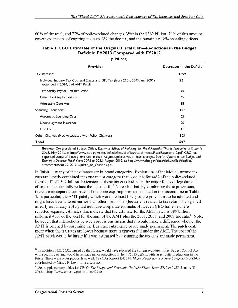
Table 1 lists the effects on the deficit of those provisions for FY2013 compared with FY2012, with the first three bulleted items listed above combined. Because most provisions change on a calendar year basis, the effect on FY2013, which ends at the end of September, reflects the effects for the first three quarters of the calendar year and not the full year’s effect. The share of the calendar year effect reflected in the fiscal year varies, however, from one provision to another. For example, the rate changes in the 2001 tax cuts would be reflected in withholding at the beginning of 2013, so that the FY2013 changes would generally capture less than a year’s effect. The effects of the lapse of the AMT patch in 2011 would largely be reflected in FY2013, because it is not generally captured in withholding, but would be collected when tax returns are filed by mid-April of 2013. Effects of the estate tax would generally be small because of the lag in filing estate tax returns.

As Table 1 shows, the fiscal cliff was largely composed of tax increases, which accounted for 80% of the total associated with legislative changes, and two-thirds of the total when including changes arising from non-policy sources. CBO also analyzed a subset of these provisions that are part of its alternative baseline. While CBO’s baseline reflects current laws (and hence assumed the Bush tax cuts would expire at the end of 2012), the alternative baseline assumed that all tax cuts except the payroll tax reduction would be extended, the AMT patch would occur, the doc fix is made each year, and the Budget Control Act automatic spending cuts do not occur, although the discretionary spending caps remain.9 This scenario, therefore, assumed that the payroll tax cuts would not be extended, that the health taxes would occur as scheduled, and that the extended emergency unemployment benefits would not be continued. The provisions that are retained as part of the alternative baseline account for $362 billion of the $607 billion total in Table 1, or

7 This tax is popularly referred to as the Medicare tax because it increases the Medicare rates and extends Medicare rates to unearned income for high-income individuals. The revenue, however, does not go to the Medicare trust fund, but is part of the financing of the health reform provisions. 8 See CRS Report R40907, Medicare Physician Payment Updates and the Sustainable Growth Rate (SGR) System, by Jim Hahn and Janemarie Mulvey. 9 See Congressional Budget Office, Updated Budget Projections: Fiscal Years 2012 to 2022, March 2012, at http://www.cbo.gov/sites/default/files/cbofiles/attachments/March2012Baseline.pdf. See CRS Report R42654, Major Fiscal Issues Before Congress in FY2013, coordinated by Mindy R. Levit, for more detail on the composition of the fiscal cliff.



60% of the total, and 72% of policy-related changes. Within the $362 billion, 79% of this amount covers extensions of expiring tax cuts, 3% the doc fix, and the remaining 18% spending effects.

Table 1. CBO Estimates of the Original Fiscal Cliff—Reductions in the Budget Deficit in FY2013 Compared with FY2012

($ billions)

Provision Decreases in the Deficit

Tax Increases $399

Individual Income Tax Cuts and Estate and Gift Tax (from 2001, 2003, and 2009) extended in 2010, and AMT Patch

221

Temporary Payroll Tax Reduction 95

Other Expiring Provisions 65

Affordable Care Act 18

Spending Reductions 102

Automatic Spending Cuts 65

Unemployment Insurance 26

Doc Fix 11

Other Changes (Not Associated with Policy Changes) 105

Total 607

Source: Congressional Budget Office, Economic Effects of Reducing the Fiscal Restraint That Is Scheduled to Occur in 2013, May 2012, at http://www.cbo.gov/sites/default/files/cbofiles/attachments/FiscalRestraint_0.pdf. CBO has reported some of these provisions in their August updates with minor changes. See An Update to the Budget and Economic Outlook: Fiscal Years 2012 to 2022, August 2012, at http://www.cbo.gov/sites/default/files/cbofiles/attachments/08-22-2012-Update_to_Outlook.pdf.

In Table 1, many of the estimates are in broad categories. Expirations of individual income tax cuts are largely combined into one major category that accounts for 44% of the policy-related fiscal cliff of $502 billion. Extension of these tax cuts had been the major focus of legislative efforts to substantially reduce the fiscal cliff.10 Note also that, by combining these provisions, there are no separate estimates of the three expiring provisions listed in the second line in Table 1. In particular, the AMT patch, which were the most likely of the provisions to be adopted and might have been altered earlier than other provisions (because it related to tax returns being filed as early as January 2013), did not have a separate estimate. However, CBO has elsewhere reported separate estimates that indicate that the estimate for the AMT patch is $89 billion, making it 40% of the total for the sum of the AMT plus the 2001, 2003, and 2009 tax cuts.11 Note, however, that interactions between provisions means that it would make a difference whether the AMT is patched by assuming the Bush tax cuts expire or are made permanent. The patch costs more when the tax rates are lower because more taxpayers fall under the AMT. The cost of the AMT patch would be larger if it was estimated by assuming the tax cuts are made permanent.

10 In addition, H.R. 5652, passed by the House, would have replaced the current sequester in the Budget Control Act with specific cuts and would have made minor reductions in the FY2013 deficit, with larger deficit reductions in the future. There were other proposals as well. See CRS Report R42654, Major Fiscal Issues Before Congress in FY2013, coordinated by Mindy R. Levit for a discussion. 11 See supplementary tables for CBO’s The Budget and Economic Outlook: Fiscal Years 2012 to 2022, January 31, 2012, at http://www.cbo.gov/publication/42910.



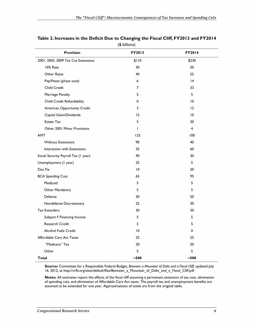
While not an official “score,” Table 2 provides detailed estimates for FY2013 and FY2014 of the deficit effects of the provisions in the original fiscal cliff by the Committee for a Responsible Federal Budget (CRFB).12 This table estimates the increase in the deficit compared with current law due to a permanent extension of expiring tax cuts, AMT patch, and extenders, and a permanent elimination of most spending cuts, including the doc fix. It also assumes that the Affordable Care Act taxes will not take effect. However, it assumes that the payroll tax and additional unemployment benefits are extended for one year. These estimates have more detail on the components of the cliff as compared with Table 1. They can also be calculated for both FY2013 and FY2014. The estimates for two fiscal years provide some insight into timing effects. These effects are important because, the earlier the effects occur, the greater the contraction in short-run demand. The estimates in Table 2 differ from Table 1, which reports the projected decreases in the deficit, including changes outside of policy choices. Hence, the total CRFB estimates are about $500 billion, the rough total of policy-related provisions in Table 1, and do not include the additional $105 billion from economic factors not related to policy.

If all taxes were reflected only in withholding, the FY2014 costs would be slightly more than a third the size of the FY2013 cost because FY2013 is only three-fourths of calendar year 2013. This pattern is seen in the rate reductions at higher-income levels. For many of the tax changes, outside of rate reductions, effects are less likely to be fully captured in withholding, and they occur when tax returns are filed. Thus a smaller effect occurs in FY2013, and effects for calendar year 2013 would in part appear with the filing of tax returns in 2014. Capital gains revenue patterns appear to measure the effect of not extending the lower rate and presumably include the expectation that gains would be realized in the last quarter of 2012 in advance of the tax rate increase (and thus reflected in 2013 with the filing of FY2012 tax returns). Very little of the estate tax revenues would be reflected in FY2013 because estate tax returns do not need to be filed until nine months after death (so that no estate tax returns would be required in FY2013 for calendar year 2013 decedents); these returns are also sometimes allowed extensions.

Because the AMT patch had already expired for 2012 and is in part reflected when returns are filed, more tax increase occurs in FY2013 than in subsequent years. Note also that the AMT patch costs more if the lower tax rates are extended, and there is also then a different distribution across fiscal years. If the tax cuts expired, the higher regular tax rates mean that fewer individuals would be on the AMT. Thus the $90 billion figure for FY2013 is the cost if current law remains in place (and higher tax rates come into play), whereas $125 billion is the cost if tax cuts are extended. In revenue estimates presented for legislative proposals, the AMT is scored last and so reflects the rate changes included in the bills. Note that some proposals would have provided a two-year AMT patch, and the second year would largely appear in FY2014. Because the Social Security payroll tax and unemployment benefits are assumed to be extended for only a year, the costs of those policies are concentrated in FY2013.

12 Committee for a Responsible Federal Budget, Between a Mountain of Debt and a Fiscal Cliff, updated July 16, 2012, at http://crfb.org/sites/default/files/Between_a_Mountain_of_Debt_and_a_Fiscal_Cliff.pdf.



Table 2. Increases in the Deficit Due to Changing the Fiscal Cliff, FY2013 and FY2014 ($ billions)

Provision FY2013 FY2014

2001, 2003, 2009 Tax Cut Extensions $110 $230

10% Rate 30 50

Other Rates 40 55

Pep/Pease (phase outs) 6 14

Child Credit 7 33

Marriage Penalty 5 5

Child Credit Refundability 0 10

American Opportunity Credit 3 12

Capital Gains/Dividends 15 10

Estate Tax 5 30

Other 2001 Minor Provisions 1 4

AMT 125 100

Without Extensions 90 40

Interaction with Extensions 35 60

Social Security Payroll Tax (1 year) 90 30

Unemployment (1 year) 25 5

Doc Fix 10 20

BCA Spending Cuts 65 95

Medicaid 5 5

Other Mandatory 5 5

Defense 30 50

Nondefense Discretionary 25 30

Tax Extenders 30 30

Subpart F Financing Income 5 5

Research Credit 5 5

Alcohol Fuels Credit 10 0

Affordable Care Act Taxes 25 25

“Medicare” Tax 20 20

Other 5 5

Total ~500 ~500

Source: Committee for a Responsible Federal Budget, Between a Mountain of Debt and a Fiscal Cliff, updated July 16, 2012, at http://crfb.org/sites/default/files/Between_a_Mountain_of_Debt_and_a_Fiscal_Cliff.pdf.

Notes: All estimates report the effects of the fiscal cliff assuming a permanent extension of tax cuts, elimination of spending cuts, and elimination of Affordable Care Act taxes. The payroll tax and unemployment benefits are assumed to be extended for one year. Approximations of totals are from the original table.



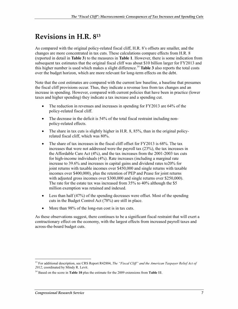
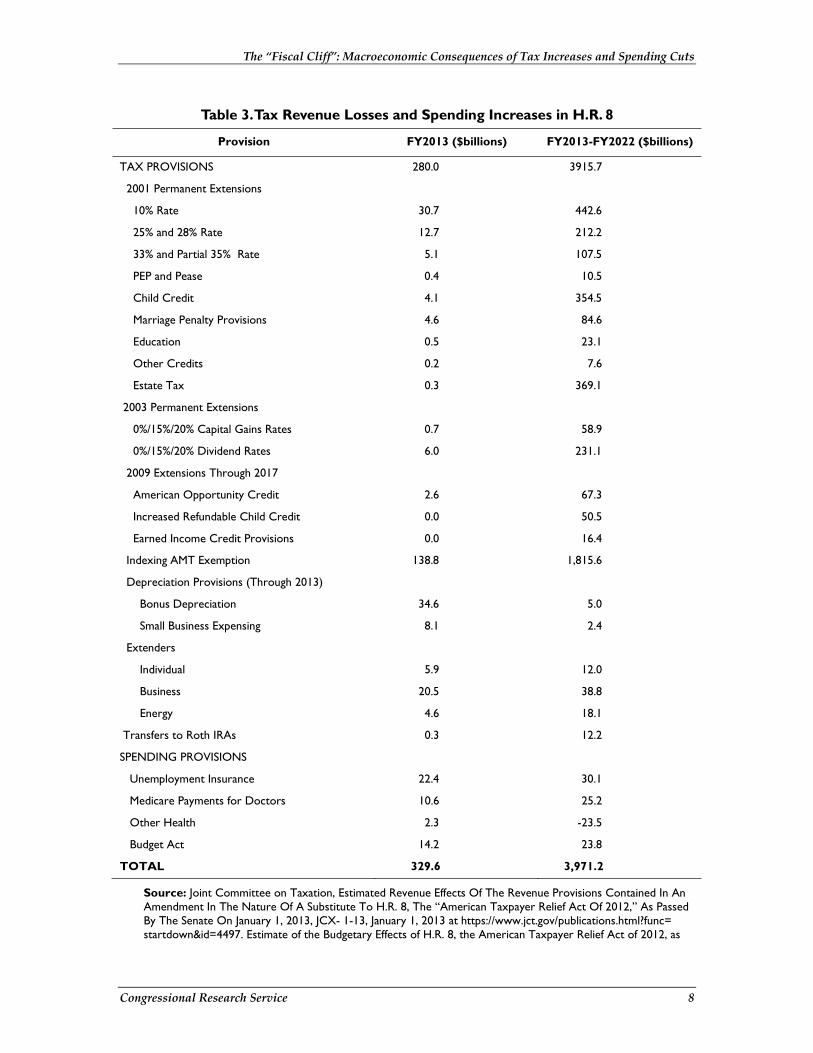
Revisions in H.R. 813 As compared with the original policy-related fiscal cliff, H.R. 8’s offsets are smaller, and the changes are more concentrated in tax cuts. These calculations compare effects from H.R. 8 (reported in detail in Table 3) to the measures in Table 1. However, there is some indication from subsequent tax estimates that the original fiscal cliff was about $10 billion larger for FY2013 and this higher number is used which makes a slight difference.14 Table 3 also reports the total costs over the budget horizon, which are more relevant for long-term effects on the debt.

Note that the cost estimates are compared with the current law baseline, a baseline that presumes the fiscal cliff provisions occur. Thus, they indicate a revenue loss from tax changes and an increase in spending. However, compared with current policies that have been in practice (lower taxes and higher spending) they indicate a tax increase and a spending cut.

• The reduction in revenues and increases in spending for FY2013 are 64% of the policy-related fiscal cliff.

• The decrease in the deficit is 54% of the total fiscal restraint including non-policy-related effects.

• The share in tax cuts is slightly higher in H.R. 8, 85%, than in the original policy-related fiscal cliff, which was 80%.

• The share of tax increases in the fiscal cliff offset for FY2013 is 68%. The tax increases that were not addressed were the payroll tax (23%), the tax increases in the Affordable Care Act (4%), and the tax increases from the 2001-2003 tax cuts for high-income individuals (4%). Rate increases (including a marginal rate increase to 39.6% and increases in capital gains and dividend rates to20% for joint returns with taxable incomes over $450,000 and single returns with taxable incomes over $400,000), plus the retention of PEP and Pease for joint returns with adjusted gross incomes over $300,000 and single returns over $250,000). The rate for the estate tax was increased from 35% to 40% although the $5 million exemption was retained and indexed.

• Less than half (47%) of the spending decreases were offset. Most of the spending cuts in the Budget Control Act (78%) are still in place.

• More than 98% of the long-run cost is in tax cuts.

As these observations suggest, there continues to be a significant fiscal restraint that will exert a contractionary effect on the economy, with the largest effects from increased payroll taxes and across-the-board budget cuts.

13 For additional description, see CRS Report R42884, The “Fiscal Cliff” and the American Taxpayer Relief Act of 2012, coordinated by Mindy R. Levit. 14 Based on the score in Table 10 plus the estimate for the 2009 extensions from Table 11.



Table 3. Tax Revenue Losses and Spending Increases in H.R. 8

Provision FY2013 ($billions) FY2013-FY2022 ($billions)

TAX PROVISIONS 280.0 3915.7

2001 Permanent Extensions

10% Rate 30.7 442.6

25% and 28% Rate 12.7 212.2

33% and Partial 35% Rate 5.1 107.5

PEP and Pease 0.4 10.5

Child Credit 4.1 354.5

Marriage Penalty Provisions 4.6 84.6

Education 0.5 23.1

Other Credits 0.2 7.6

Estate Tax 0.3 369.1

2003 Permanent Extensions

0%/15%/20% Capital Gains Rates 0.7 58.9

0%/15%/20% Dividend Rates 6.0 231.1

2009 Extensions Through 2017

American Opportunity Credit 2.6 67.3

Increased Refundable Child Credit 0.0 50.5

Earned Income Credit Provisions 0.0 16.4

Indexing AMT Exemption 138.8 1,815.6

Depreciation Provisions (Through 2013)

Bonus Depreciation 34.6 5.0

Small Business Expensing 8.1 2.4

Extenders

Individual 5.9 12.0

Business 20.5 38.8

Energy 4.6 18.1

Transfers to Roth IRAs 0.3 12.2

SPENDING PROVISIONS

Unemployment Insurance 22.4 30.1

Medicare Payments for Doctors 10.6 25.2

Other Health 2.3 -23.5

Budget Act 14.2 23.8

TOTAL 329.6 3,971.2

Source: Joint Committee on Taxation, Estimated Revenue Effects Of The Revenue Provisions Contained In An Amendment In The Nature Of A Substitute To H.R. 8, The “American Taxpayer Relief Act Of 2012,” As Passed By The Senate On January 1, 2013, JCX- 1-13, January 1, 2013 at https://www.jct.gov/publications.html?func=startdown&id=4497. Estimate of the Budgetary Effects of H.R. 8, the American Taxpayer Relief Act of 2012, as



passed by the Senate on January 1, 2013, at http://www.cbo.gov/sites/default/files/cbofiles/attachments/American%20Taxpayer%20Relief%20Act.pdf.

Note: The Congressional Budget Office allocates by revenues and outlays, while the Joint Committee on Taxation includes outlay effects (refundable taxes) in revenues.

Aggregate Short-Run Effects of the Original Fiscal Cliff The contraction in aggregate demand resulting from the original fiscal cliff, according to standard economic analysis, would have reduced output and employment in the economy.15 A number of estimates and comments suggested that the fiscal cliff, which CBO expected to reduce the deficit by 5.1% of output in calendar year 2013, would also reduce aggregate demand and have a large negative effect on the economy in the short run. Chairman of the Federal Reserve Ben Bernanke indicated in testimony before Congress that, while there is a need for long-run debt sustainability, the tax increases and spending cuts occurring in 2013 could endanger the recovery.16 The International Monetary Fund, an organization that often stresses the need for reducing debt levels, expressed concern that the fiscal cliff would damage the U.S. and worldwide economy and recommended that the deficit decrease by only 1% of GDP (output), about a fifth of the fiscal cliff.17 The IMF also identified the fiscal cliff as the most important risk to global recovery:

In the short term, the main risk relates to the possibility of excessive fiscal tightening in the United States, given recent political gridlock. In the extreme, if policymakers fail to reach consensus on extending some temporary tax cuts and reversing deep automatic spending cuts, the U.S. structural fiscal deficit could decline by more than 4 percentage points of GDP

15 The discussion of economic effects in this section may be seen as a mainstream view as reflected in the analysis of the Congressional Budget Office, the International Monetary Fund, the Federal Reserve Board, other government forecasters, and private forecasters. There are prominent economists who disagree that fiscal stimulus is effective or that the fiscal cliff is an important issue for the demand side and unemployment. See, for example, Robert J. Barro, “Keynesian Economics vs. Regular Economics,” Wall Street Journal, August 24, 2011, and John B. Taylor, “An Empirical Analysis of the Revision of Fiscal Activism in the 2000s,” Journal of Economic Literature, vol. 49, September 2011, pp. 686-702. For a discussion of the various models that have been developed that reject fiscal stimulus (primarily by academic economists) as well as modifications that have affected some modeling of a fiscal stimulus, see N. Gregory Mankiw, “The Macroeconomist as Scientist and Engineer,” The Journal of Economic Perspectives, vol. 20, fall 2006, pp. 29-46. There are also arguments that countries have grown after deficit reductions (sometimes referred to as fiscal consolidations), although the examples cited generally began at full employment, rather than the circumstances facing the United States. For a discussion of the intertemporal models referenced by Barro, see CRS Report RL31949, Issues in Dynamic Revenue Estimating, by Jane G. Gravelle. For a review of the evidence on fiscal consolidation, see CRS Report R41849, Can Contractionary Fiscal Policy Be Expansionary? by Jane G. Gravelle and Thomas L. Hungerford. Note that recently a number of countries taking the path of fiscal consolidation, either by choice or after outside pressure, have seen growth suffer. See, for example, the discussion of Great Britain, “Economy to Shrink in 2012 as Quick Austerity Hurts – NIESR,” Reuters, August 3, 2012, at http://www.reuters.com/article/2012/08/02/britain-economy-niesr-idUSL6E8J2JWK20120802. In general, the constraints of the European Union, the contractionary policies now being undertaken, and the fragility of debt in some countries have exacerbated the problems of the world, including the United States. See Mark Zandi, U.S. Macro Outlook: Policymakers Must Get It Right, Moody’s Analytics, at http://www.economy.com/dismal/article_free.asp?cid=232471&src=mark-zandi. 16 Ben S. Bernanke, Chairman, Board of Governors of the Federal Reserve, Testimony before the Senate Committee on Banking, Housing and Urban Affairs, July 17, 2012, at http://www.federalreserve.gov/newsevents/testimony/bernanke20120717a1.pdf. 17 International Monetary Fund Fiscal Monitor, Nurturing Credibility While Managing Risks to Growth, July 16, 2012, at http://www.imf.org/external/pubs/ft/fm/2012/update/02/pdf/0712.pdf.



in 2013. U.S. growth would then stall next year, with significant spillovers to the rest of the world.18

In its May 2012 report, CBO considered a range of estimates.19 The midpoint of those estimates indicated that, if the fiscal cliff occurred, GDP would actually contract by 1.3% in the first half of calendar year 2013, with growth of 2.3% in the second half, for an overall growth over the year of 0.5%. With elimination of the fiscal cliff, their midpoint estimate indicated that growth would be 4.4% (5.3% in the first half and 3.4% in the second half). Thus, the fiscal cliff would be projected to lead to a reduction in output of 3.9%. CBO projected that not eliminating the fiscal cliff would have increased unemployment by 2 million. CBO’s analysis noted some uncertainty about these effects. Although the midpoint estimate was a reduction of 3.9% of output, the range of potential effects of the fiscal cliff in the CBO analysis was set at 0.9% to 6.8% of output. Thus, the effects might have been considerably smaller, but they also could have been much larger.20 CBO did not explicitly analyze the fiscal cliff in its August 2012 budget update, but it did project a larger initial contraction of 2.9% in the first half of 2013 under current law, followed by a 1.9% increase, with unemployment reaching 9.1% by the last quarter. This contraction would qualify as a recession. The overall difference in output was about 5%.21

Other forecasters projected similar effects, although they varied somewhat in what they included in the fiscal cliff. Mark Zandi of Moody’s Analytics estimated a fiscal cliff deficit reduction at 4.6% of output, producing a contraction of 3.6% of output.22 Morgan Stanley reported a deficit effect of 5% of output, for a contraction of 5% of output, and Goldman Sachs reported a deficit effect of 4% of output, for a contraction of 4% of output.23 IHS Global Insight assumed that the fiscal cliff would be avoided in its forecasts but indicated that going over the fiscal cliff would lead to recession.24

Differential Effects of the Components of the Fiscal Cliff The principal reason the fiscal cliff had such a potential to slow and even contract the economy in the short run was its size. At a deficit reduction of 5% of GDP, the changes in policies constituted a large contractionary effect. However, the effect of the fiscal cliff on the economy also depends

18 International Monetary Fund World Economic Outlook Update, New Setbacks, Further Policy Action Needed, July 16, 2012, p. 5, at http://www.imf.org/external/pubs/ft/weo/2012/update/02/pdf/0712.pdf. 19 Congressional Budget Office, Economic Effects of Reducing the Fiscal Restraint That Is Scheduled to Occur in 2013, May 2012, at http://www.cbo.gov/sites/default/files/cbofiles/attachments/FiscalRestraint_0.pdf. 20 CBO’s ranges reflect the range of estimated effects from a variety of sources. For a further discussion of sources, see Felix Reichling and Charles Whalen, Assessing the Short-Term Effects on Output of Changes in Federal Fiscal Policies, CBO Working Paper 2012-08, May 2012, at http://www.cbo.gov/sites/default/files/cbofiles/attachments/WorkingPaper2012-08-Effects_of_Fiscal_Policies.pdf. 21 Congressional Budget Office, An Update to the Budget and Economic Outlook: Fiscal Years 2012 to 2022, August 2012, at http://www.cbo.gov/sites/default/files/cbofiles/attachments/08-22-2012-Update_to_Outlook.pdf. 22 Mark Zandi, U.S. Macro Outlook: Policymakers Must Get It Right, Moody’s Analytics, July 16, 2012, at http://www.economy.com/dismal/article_free.asp?cid=232471&src=mark-zandi. 23 As reported in Committee for a Responsible Federal Budget, Between a Mountain of Debt and a Fiscal Cliff, updated July 16, 2012, at http://crfb.org/sites/default/files/Between_a_Mountain_of_Debt_and_a_Fiscal_Cliff.pdf. 24 IHS Global Insight, U.S. Economic Outlook, July 2012, p. 3.



on the mix of policies. The differential contractionary effects of different elements of the fiscal cliff could have played a role in balancing short-term and long-run objectives.

The contractionary effect of spending cuts and tax increases occurs because these changes reduce spending and contract demand. Reductions in direct spending directly reduce demand, and increases in taxes or decreases in transfers may partly cause a reduction in savings and partly a reduction in private spending. This decreased demand causes fewer workers to be hired and less output to be produced; some of the resulting reduced income also reduces spending, with another round of contraction. The outcome of these successive rounds of reduced spending are called multipliers. There are forces in the economy that limit the effects. For example, with a relatively small contraction for an economy at full employment, the multiplier could be close to zero because the contraction may lower interest rates or prices or both without any real output effects. Even with an underemployed economy, there are aspects that dampen the effects on the economy. For example, part of each round of decreased income reduces savings rather than spending, or some part of the contraction in demand decreases imports rather than domestic production, or some of the contraction drives down interest rates and increases private investment. (During this recession and recovery, there has been little evidence of fiscal policies altering interest rates.)

The CBO projections initially indicated an aggregate multiplier for the fiscal cliff of 0.76 (a 3.9% contraction in output divided by a 5.1% decrease in the deficit relative to output). Zandi’s multiplier is about the same at 0.78 (3.6% divided 4.6%), whereas the other two forecasters indicate multipliers of one. CBO’s later projections indicated a multiplier closer to one.

A crucial feature that causes different policies to have different effects is the size and speed of the first round of spending cuts. If the federal government decreases direct purchases of goods and services, spending is reduced by 100% of that amount. However, if the government increases taxes, individuals would reduce spending by only a fraction of that tax increase (with savings falling as well). If only half of a tax increase decreases spending, a tax multiplier is half as large as a spending multiplier. Reduced transfers and tax increases for low-income individuals are likely to reduce spending because these individuals are usually liquidity constrained (unable to borrow to meet their spending objectives). Higher-income individuals are more likely to reduce spending by a smaller share of a tax increase, and businesses are also unlikely to change their spending very much. Reductions in transfers to state and local governments may also partially reduce savings, although these governments are now generally financially constrained and may be more likely to reduce spending.

There are also issues of timing. If spending increases are authorized but cannot take place quickly, their effect would be delayed. This concern was a significant one in considering spending increases in 2009, particularly with respect to infrastructure, where a planning period might have been needed. Of course, that timing issue would be different because the policy in this case involves not a spending increase, which could take some time but avoiding a spending cut. Presumably, cuts could be made more quickly than increases. (Note that in measuring the fiscal cliff, CBO projects spending changes under the BCA, not changes in budget authority.)

The general patterns of differentials can be seen in CBO’s analysis of the effects of the 2009 stimulus (tax cuts and spending increases to expand the economy) as shown in Table 4. Considering the midpoint of multipliers in the last column, changes in federal spending have a higher multiplier than a low-to-middle-income tax change. Tax changes for higher-income individuals and businesses have the smallest multipliers. Transfers to individuals (such as



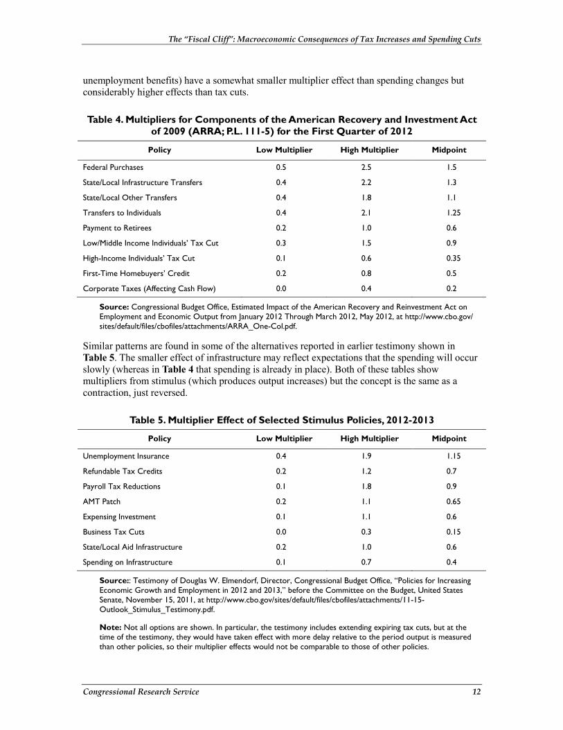
unemployment benefits) have a somewhat smaller multiplier effect than spending changes but considerably higher effects than tax cuts.

Table 4. Multipliers for Components of the American Recovery and Investment Act of 2009 (ARRA; P.L. 111-5) for the First Quarter of 2012

Policy Low Multiplier High Multiplier Midpoint

Federal Purchases 0.5 2.5 1.5

State/Local Infrastructure Transfers 0.4 2.2 1.3

State/Local Other Transfers 0.4 1.8 1.1

Transfers to Individuals 0.4 2.1 1.25

Payment to Retirees 0.2 1.0 0.6

Low/Middle Income Individuals’ Tax Cut 0.3 1.5 0.9

High-Income Individuals’ Tax Cut 0.1 0.6 0.35

First-Time Homebuyers’ Credit 0.2 0.8 0.5

Corporate Taxes (Affecting Cash Flow) 0.0 0.4 0.2

Source: Congressional Budget Office, Estimated Impact of the American Recovery and Reinvestment Act on Employment and Economic Output from January 2012 Through March 2012, May 2012, at http://www.cbo.gov/sites/default/files/cbofiles/attachments/ARRA_One-Col.pdf.

Similar patterns are found in some of the alternatives reported in earlier testimony shown in Table 5. The smaller effect of infrastructure may reflect expectations that the spending will occur slowly (whereas in Table 4 that spending is already in place). Both of these tables show multipliers from stimulus (which produces output increases) but the concept is the same as a contraction, just reversed.

Table 5. Multiplier Effect of Selected Stimulus Policies, 2012-2013

Policy Low Multiplier High Multiplier Midpoint

Unemployment Insurance 0.4 1.9 1.15

Refundable Tax Credits 0.2 1.2 0.7

Payroll Tax Reductions 0.1 1.8 0.9

AMT Patch 0.2 1.1 0.65

Expensing Investment 0.1 1.1 0.6

Business Tax Cuts 0.0 0.3 0.15

State/Local Aid Infrastructure 0.2 1.0 0.6

Spending on Infrastructure 0.1 0.7 0.4

Source:: Testimony of Douglas W. Elmendorf, Director, Congressional Budget Office, “Policies for Increasing Economic Growth and Employment in 2012 and 2013,” before the Committee on the Budget, United States Senate, November 15, 2011, at http://www.cbo.gov/sites/default/files/cbofiles/attachments/11-15-Outlook_Stimulus_Testimony.pdf.

Note: Not all options are shown. In particular, the testimony includes extending expiring tax cuts, but at the time of the testimony, they would have taken effect with more delay relative to the period output is measured than other policies, so their multiplier effects would not be comparable to those of other policies.



CBO’s report on the fiscal cliff also contained additional estimates that allow separate multipliers for different components of the fiscal cliff. CBO indicates that the fiscal cliff with a deficit decrease at 5.1% of GDP comparing calendar 2012 and 2013 will result in a decrease in output of 3.9%. CBO also estimates that the decreases in the deficit under the alternative baseline compared with current law, which accounts for 3% of GDP, would lead to an offsetting gain of 1.6% of output, with the remainder of the fiscal cliff (including non-policy-related amounts) leading to a 2.3% reduction. These estimates imply that these largely tax changes have a multiplier of 0.5 (1.6% divided by 3%) and the other provisions a multiplier of 1.1 (2.3% divided by 2.1%). In its August report, CBO estimates a similar reduction comparing the current law baseline and the alternative scenario (-0.5% versus 1.7% for a net increase of 2.2%).25 Apparently, CBO’s August update compared with the May analysis indicates a gloomier outlook in general.

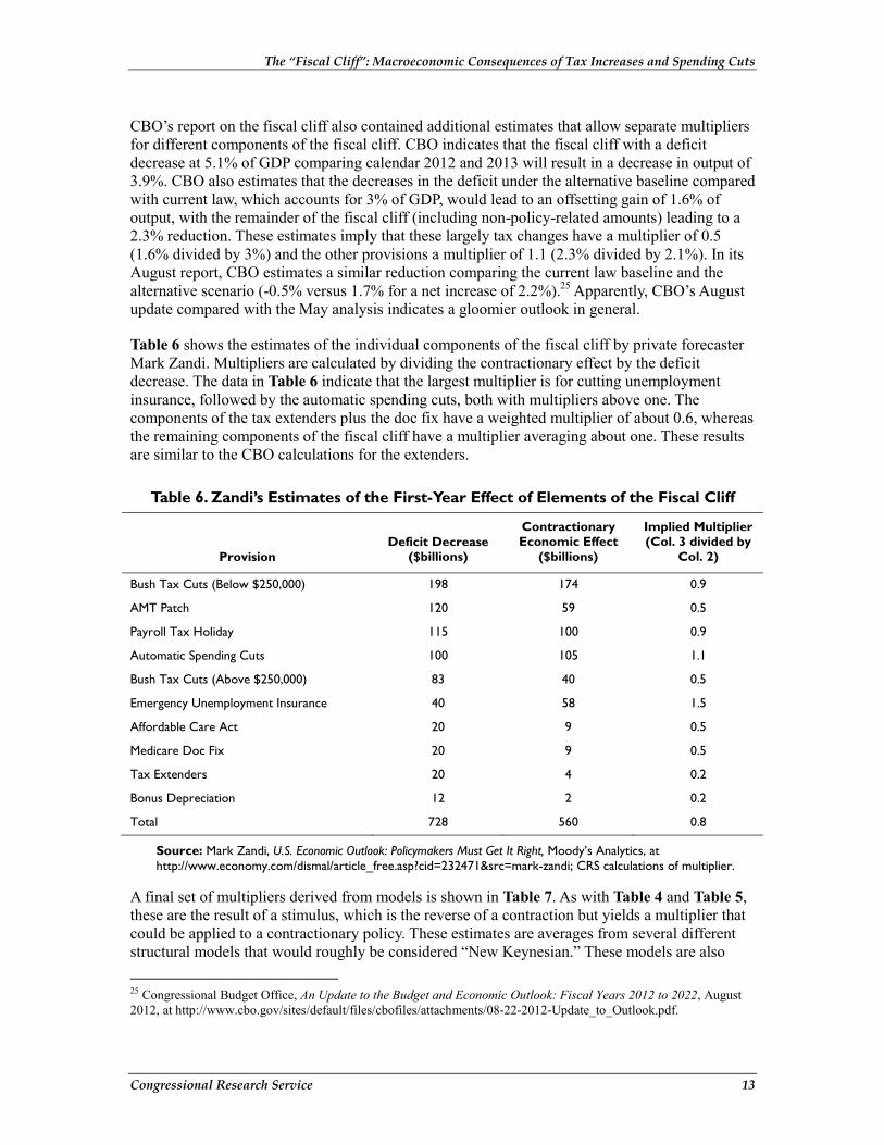
Table 6 shows the estimates of the individual components of the fiscal cliff by private forecaster Mark Zandi. Multipliers are calculated by dividing the contractionary effect by the deficit decrease. The data in Table 6 indicate that the largest multiplier is for cutting unemployment insurance, followed by the automatic spending cuts, both with multipliers above one. The components of the tax extenders plus the doc fix have a weighted multiplier of about 0.6, whereas the remaining components of the fiscal cliff have a multiplier averaging about one. These results are similar to the CBO calculations for the extenders.

Table 6. Zandi’s Estimates of the First-Year Effect of Elements of the Fiscal Cliff

Provision Deficit Decrease

($billions)

Contractionary Economic Effect

($billions)

Implied Multiplier (Col. 3 divided by

Col. 2)

Bush Tax Cuts (Below $250,000) 198 174 0.9

AMT Patch 120 59 0.5

Payroll Tax Holiday 115 100 0.9

Automatic Spending Cuts 100 105 1.1

Bush Tax Cuts (Above $250,000) 83 40 0.5

Emergency Unemployment Insurance 40 58 1.5

Affordable Care Act 20 9 0.5

Medicare Doc Fix 20 9 0.5

Tax Extenders 20 4 0.2

Bonus Depreciation 12 2 0.2

Total 728 560 0.8

Source: Mark Zandi, U.S. Economic Outlook: Policymakers Must Get It Right, Moody’s Analytics, at http://www.economy.com/dismal/article_free.asp?cid=232471&src=mark-zandi; CRS calculations of multiplier.

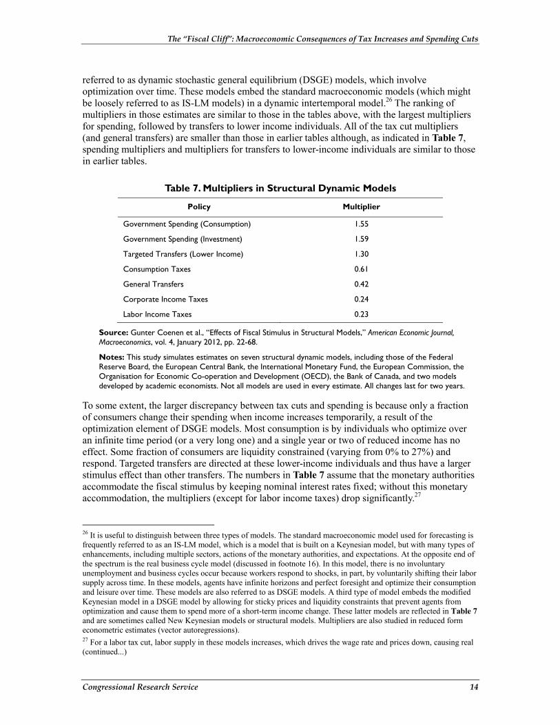
A final set of multipliers derived from models is shown in Table 7. As with Table 4 and Table 5, these are the result of a stimulus, which is the reverse of a contraction but yields a multiplier that could be applied to a contractionary policy. These estimates are averages from several different structural models that would roughly be considered “New Keynesian.” These models are also

25 Congressional Budget Office, An Update to the Budget and Economic Outlook: Fiscal Years 2012 to 2022, August 2012, at http://www.cbo.gov/sites/default/files/cbofiles/attachments/08-22-2012-Update_to_Outlook.pdf.



referred to as dynamic stochastic general equilibrium (DSGE) models, which involve optimization over time. These models embed the standard macroeconomic models (which might be loosely referred to as IS-LM models) in a dynamic intertemporal model.26 The ranking of multipliers in those estimates are similar to those in the tables above, with the largest multipliers for spending, followed by transfers to lower income individuals. All of the tax cut multipliers (and general transfers) are smaller than those in earlier tables although, as indicated in Table 7, spending multipliers and multipliers for transfers to lower-income individuals are similar to those in earlier tables.

Table 7. Multipliers in Structural Dynamic Models

Policy Multiplier

Government Spending (Consumption) 1.55

Government Spending (Investment) 1.59

Targeted Transfers (Lower Income) 1.30

Consumption Taxes 0.61

General Transfers 0.42

Corporate Income Taxes 0.24

Labor Income Taxes 0.23

Source: Gunter Coenen et al., “Effects of Fiscal Stimulus in Structural Models,” American Economic Journal, Macroeconomics, vol. 4, January 2012, pp. 22-68.

Notes: This study simulates estimates on seven structural dynamic models, including those of the Federal Reserve Board, the European Central Bank, the International Monetary Fund, the European Commission, the Organisation for Economic Co-operation and Development (OECD), the Bank of Canada, and two models developed by academic economists. Not all models are used in every estimate. All changes last for two years.

To some extent, the larger discrepancy between tax cuts and spending is because only a fraction of consumers change their spending when income increases temporarily, a result of the optimization element of DSGE models. Most consumption is by individuals who optimize over an infinite time period (or a very long one) and a single year or two of reduced income has no effect. Some fraction of consumers are liquidity constrained (varying from 0% to 27%) and respond. Targeted transfers are directed at these lower-income individuals and thus have a larger stimulus effect than other transfers. The numbers in Table 7 assume that the monetary authorities accommodate the fiscal stimulus by keeping nominal interest rates fixed; without this monetary accommodation, the multipliers (except for labor income taxes) drop significantly.27

26 It is useful to distinguish between three types of models. The standard macroeconomic model used for forecasting is frequently referred to as an IS-LM model, which is a model that is built on a Keynesian model, but with many types of enhancements, including multiple sectors, actions of the monetary authorities, and expectations. At the opposite end of the spectrum is the real business cycle model (discussed in footnote 16). In this model, there is no involuntary unemployment and business cycles occur because workers respond to shocks, in part, by voluntarily shifting their labor supply across time. In these models, agents have infinite horizons and perfect foresight and optimize their consumption and leisure over time. These models are also referred to as DSGE models. A third type of model embeds the modified Keynesian model in a DSGE model by allowing for sticky prices and liquidity constraints that prevent agents from optimization and cause them to spend more of a short-term income change. These latter models are reflected in Table 7 and are sometimes called New Keynesian models or structural models. Multipliers are also studied in reduced form econometric estimates (vector autoregressions). 27 For a labor tax cut, labor supply in these models increases, which drives the wage rate and prices down, causing real (continued...)



In general, these models are more popular with academics and tend to not be as influential among policymakers and private forecasters. Some researchers raise questions about whether the spending behavior in these models is consistent with direct evidence.28

Multipliers are also directly estimated using multiple time series regressions (statistical studies that examine changes in deficits and output over time), but often these studies focus on government spending (where the policies are more uniform and the first round can be presumed to be spent) or do not distinguish among the types of policies (although theory suggests that tax cut multipliers should be smaller).29 An important issue that has been raised about these studies (and about estimates of multipliers in general) is that multipliers should be estimated in a way that allows different multipliers in booms and recessions. One recent study indicated that the government spending multiplier was between 0 and 0.5 during expansions and between 1 and 1.5 in recessions.30

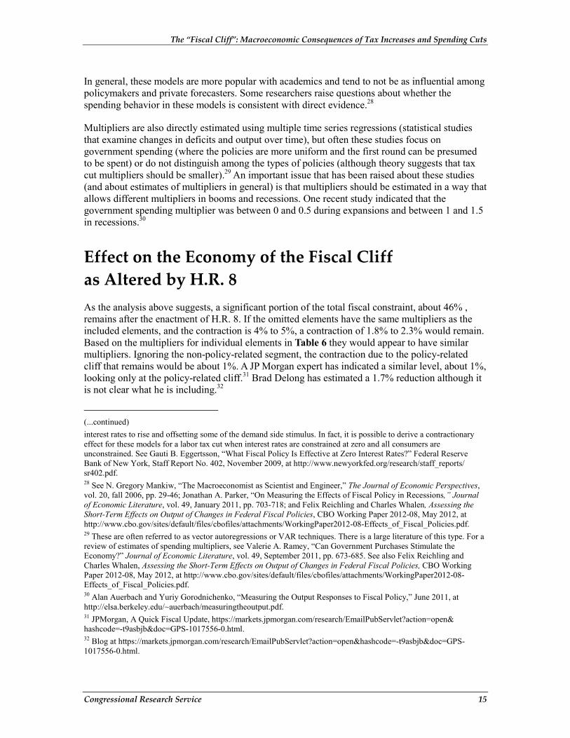
Effect on the Economy of the Fiscal Cliff as Altered by H.R. 8 As the analysis above suggests, a significant portion of the total fiscal constraint, about 46% , remains after the enactment of H.R. 8. If the omitted elements have the same multipliers as the included elements, and the contraction is 4% to 5%, a contraction of 1.8% to 2.3% would remain. Based on the multipliers for individual elements in Table 6 they would appear to have similar multipliers. Ignoring the non-policy-related segment, the contraction due to the policy-related cliff that remains would be about 1%. A JP Morgan expert has indicated a similar level, about 1%, looking only at the policy-related cliff.31 Brad Delong has estimated a 1.7% reduction although it is not clear what he is including.32

(...continued) interest rates to rise and offsetting some of the demand side stimulus. In fact, it is possible to derive a contractionary effect for these models for a labor tax cut when interest rates are constrained at zero and all consumers are unconstrained. See Gauti B. Eggertsson, “What Fiscal Policy Is Effective at Zero Interest Rates?” Federal Reserve Bank of New York, Staff Report No. 402, November 2009, at http://www.newyorkfed.org/research/staff_reports/sr402.pdf. 28 See N. Gregory Mankiw, “The Macroeconomist as Scientist and Engineer,” The Journal of Economic Perspectives, vol. 20, fall 2006, pp. 29-46; Jonathan A. Parker, “On Measuring the Effects of Fiscal Policy in Recessions,” Journal of Economic Literature, vol. 49, January 2011, pp. 703-718; and Felix Reichling and Charles Whalen, Assessing the Short-Term Effects on Output of Changes in Federal Fiscal Policies, CBO Working Paper 2012-08, May 2012, at http://www.cbo.gov/sites/default/files/cbofiles/attachments/WorkingPaper2012-08-Effects_of_Fiscal_Policies.pdf. 29 These are often referred to as vector autoregressions or VAR techniques. There is a large literature of this type. For a review of estimates of spending multipliers, see Valerie A. Ramey, “Can Government Purchases Stimulate the Economy?” Journal of Economic Literature, vol. 49, September 2011, pp. 673-685. See also Felix Reichling and Charles Whalen, Assessing the Short-Term Effects on Output of Changes in Federal Fiscal Policies, CBO Working Paper 2012-08, May 2012, at http://www.cbo.gov/sites/default/files/cbofiles/attachments/WorkingPaper2012-08-Effects_of_Fiscal_Policies.pdf. 30 Alan Auerbach and Yuriy Gorodnichenko, “Measuring the Output Responses to Fiscal Policy,” June 2011, at http://elsa.berkeley.edu/~auerbach/measuringtheoutput.pdf. 31 JPMorgan, A Quick Fiscal Update, https://markets.jpmorgan.com/research/EmailPubServlet?action=open&hashcode=-t9asbjb&doc=GPS-1017556-0.html. 32 Blog at https://markets.jpmorgan.com/research/EmailPubServlet?action=open&hashcode=-t9asbjb&doc=GPS-1017556-0.html.



Implications for Policy Choices The policies that have received significant legislative attention during 2012 that would change the size of the fiscal cliff—extending the expiring tax cuts—are a majority of the fiscal cliff but a minority of the economic effects, although the economic effects are still notable. According to the implications of the CBO estimates of the effects of the alternative fiscal scenario (which largely extends the expiring tax cuts), the provisions in the alternative scenario are responsible for 60% of the fiscal cliff but 40% of the contraction. Hence extending the expiring tax cuts eliminates less than half of the projected contraction in the economy due to the fiscal cliff.

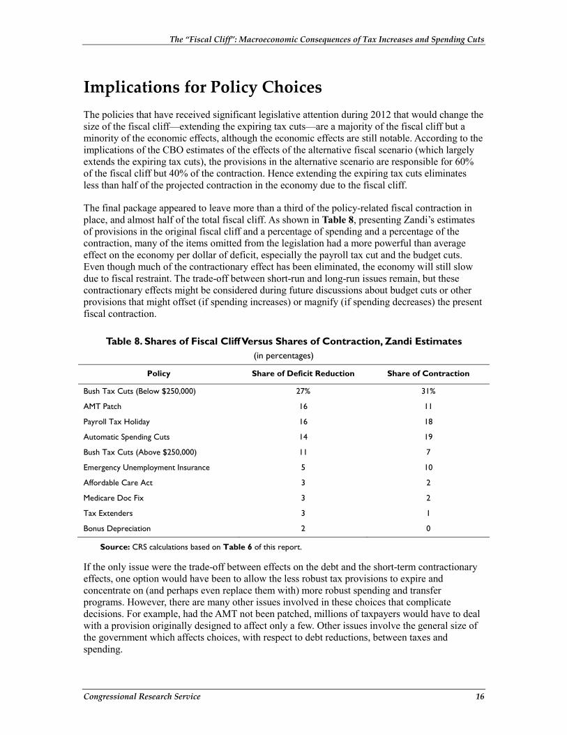
The final package appeared to leave more than a third of the policy-related fiscal contraction in place, and almost half of the total fiscal cliff. As shown in Table 8, presenting Zandi’s estimates of provisions in the original fiscal cliff and a percentage of spending and a percentage of the contraction, many of the items omitted from the legislation had a more powerful than average effect on the economy per dollar of deficit, especially the payroll tax cut and the budget cuts. Even though much of the contractionary effect has been eliminated, the economy will still slow due to fiscal restraint. The trade-off between short-run and long-run issues remain, but these contractionary effects might be considered during future discussions about budget cuts or other provisions that might offset (if spending increases) or magnify (if spending decreases) the present fiscal contraction.

Table 8. Shares of Fiscal Cliff Versus Shares of Contraction, Zandi Estimates (in percentages)

Policy Share of Deficit Reduction Share of Contraction

Bush Tax Cuts (Below $250,000) 27% 31%

AMT Patch 16 11

Payroll Tax Holiday 16 18

Automatic Spending Cuts 14 19

Bush Tax Cuts (Above $250,000) 11 7

Emergency Unemployment Insurance 5 10

Affordable Care Act 3 2

Medicare Doc Fix 3 2

Tax Extenders 3 1

Bonus Depreciation 2 0

Source: CRS calculations based on Table 6 of this report.

If the only issue were the trade-off between effects on the debt and the short-term contractionary effects, one option would have been to allow the less robust tax provisions to expire and concentrate on (and perhaps even replace them with) more robust spending and transfer programs. However, there are many other issues involved in these choices that complicate decisions. For example, had the AMT not been patched, millions of taxpayers would have to deal with a provision originally designed to affect only a few. Other issues involve the general size of the government which affects choices, with respect to debt reductions, between taxes and spending.



Appendix. Legislative Proposals Considered in 2012 The focus of legislative change that would have affected the fiscal cliff during 2012 was largely on the expiring tax cuts. Although spending cuts have been the subject of legislative proposals, these proposals were largely about reordering spending rather than affecting the magnitude of the cuts.33 Proposals in both the House and Senate addressed the expiring tax cuts from 2001, 2003, and 2009, which had been extended in 2010, along with the AMT patch, which together contributed $221 billion (44%) of the policy-related fiscal cliff. A separate bill to address the AMT patch and the “extenders” had also been approved by the Senate Finance Committee.

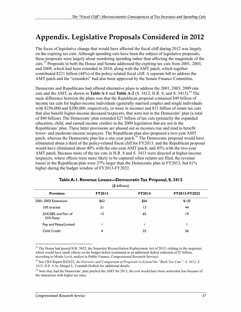
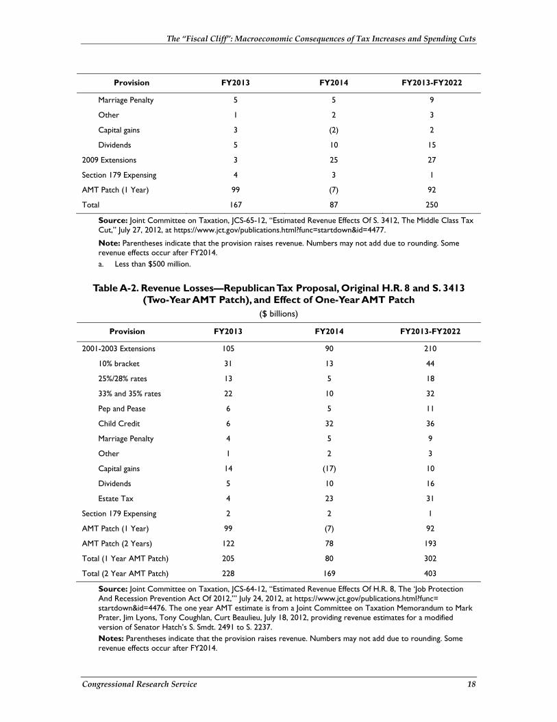
Democrats and Republicans had offered alternative plans to address the 2001, 2003, 2009 rate cuts and the AMT, as shown in Table A-1 and Table A-2 (S. 3412; H.R. 8, and S. 3413).34 The main difference between the plans was that the Republican proposal contained $49 billion of income tax cuts for higher-income individuals (generally married couples and single individuals with $250,000 and $200,000, respectively, or more in income) and $31 billion of estate tax cuts that also benefit higher-income deceased taxpayers, that were not in the Democrats’ plan (a total of $80 billion). The Democrats’ plan extended $27 billion of tax cuts (primarily the expanded education, child, and earned income credits) in the 2009 legislation that are not in the Republicans’ plan. These latter provisions are phased out as incomes rise and tend to benefit lower- and moderate-income taxpayers. The Republican plan also proposed a two-year AMT patch, whereas the Democratic plan has a one-year patch.35 The Democratic proposal would have eliminated about a third of the policy-related fiscal cliff for FY2013, and the Republican proposal would have eliminated about 40% with the one-year AMT patch, and 45% with the two-year AMT patch. Because more of the tax cuts in H.R. 8 and S. 3413 were directed at higher-income taxpayers, where effects were more likely to be captured when returns are filed, the revenue losses in the Republican plan were 37% larger than the Democratic plan in FY2013, but 61% higher during the budget window of FY2013-FY2022.

Table A-1. Revenue Losses—Democratic Tax Proposal, S. 3412 ($ billions)

Provision FY2013 FY2014 FY2013-FY2022

2001-2003 Extensions $62 $66 $130

10% bracket 31 13 44

25%/28% and Part of 33% Rates

13 65 19

Pep and Pease/Limited a a 1

Child Credit 4 32 36

33 The House had passed H.R. 5652, the Sequester Reconciliation Replacement Act of 2012, relating to the sequester, which would have small effects on the budget deficit (estimated at an additional deficit reduction of $7 billion, according to Mindy Levit, analyst in Public Finance, Congressional Research Service). 34 See CRS Report R42622, An Overview and Comparison of Proposals to Extend the “Bush Tax Cuts”: S. 3412, S. 3413, H.R. 8, by Margot L. Crandall-Hollick for additional details. 35 Note that, had the Democrats’ plan patched the AMT for 2013, the cost would have been somewhat less because of the interaction with higher tax rates.




Marriage Penalty 5 5 9

Other 1 2 3

Capital gains 3 (2) 2

Dividends 5 10 15

2009 Extensions 3 25 27

Section 179 Expensing 4 3 1

AMT Patch (1 Year) 99 (7) 92

Total 167 87 250

Source: Joint Committee on Taxation, JCS-65-12, “Estimated Revenue Effects Of S. 3412, The Middle Class Tax Cut,” July 27, 2012, at https://www.jct.gov/publications.html?func=startdown&id=4477.

Note: Parentheses indicate that the provision raises revenue. Numbers may not add due to rounding. Some revenue effects occur after FY2014. a. Less than $500 million.

Table A-2. Revenue Losses—Republican Tax Proposal, Original H.R. 8 and S. 3413 (Two-Year AMT Patch), and Effect of One-Year AMT Patch

($ billions)


2001-2003 Extensions 105 90 210

10% bracket 31 13 44

25%/28% rates 13 5 18

33% and 35% rates 22 10 32

Pep and Pease 6 5 11

Child Credit 6 32 36

Marriage Penalty 4 5 9

Other 1 2 3

Capital gains 14 (17) 10

Dividends 5 10 16

Estate Tax 4 23 31

Section 179 Expensing 2 2 1

AMT Patch (1 Year) 99 (7) 92

AMT Patch (2 Years) 122 78 193

Total (1 Year AMT Patch) 205 80 302

Total (2 Year AMT Patch) 228 169 403

Source: Joint Committee on Taxation, JCS-64-12, “Estimated Revenue Effects Of H.R. 8, The ‘Job Protection And Recession Prevention Act Of 2012,’” July 24, 2012, at https://www.jct.gov/publications.html?func=startdown&id=4476. The one year AMT estimate is from a Joint Committee on Taxation Memorandum to Mark Prater, Jim Lyons, Tony Coughlan, Curt Beaulieu, July 18, 2012, providing revenue estimates for a modified version of Senator Hatch’s S. Smdt. 2491 to S. 2237. Notes: Parentheses indicate that the provision raises revenue. Numbers may not add due to rounding. Some revenue effects occur after FY2014.



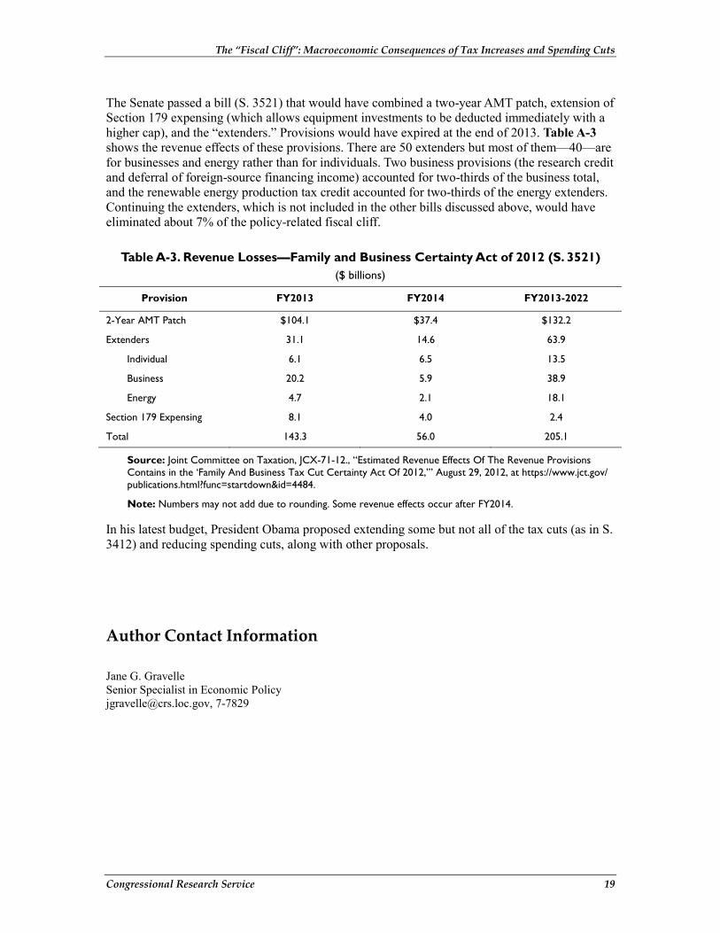
The Senate passed a bill (S. 3521) that would have combined a two-year AMT patch, extension of Section 179 expensing (which allows equipment investments to be deducted immediately with a higher cap), and the “extenders.” Provisions would have expired at the end of 2013. Table A-3 shows the revenue effects of these provisions. There are 50 extenders but most of them—40—are for businesses and energy rather than for individuals. Two business provisions (the research credit and deferral of foreign-source financing income) accounted for two-thirds of the business total, and the renewable energy production tax credit accounted for two-thirds of the energy extenders. Continuing the extenders, which is not included in the other bills discussed above, would have eliminated about 7% of the policy-related fiscal cliff.

Table A-3. Revenue Losses—Family and Business Certainty Act of 2012 (S. 3521) ($ billions)

Provision FY2013 FY2014 FY2013-2022

2-Year AMT Patch $104.1 $37.4 $132.2

Extenders 31.1 14.6 63.9

Individual 6.1 6.5 13.5

Business 20.2 5.9 38.9

Energy 4.7 2.1 18.1

Section 179 Expensing 8.1 4.0 2.4

Total 143.3 56.0 205.1

Source: Joint Committee on Taxation, JCX-71-12., “Estimated Revenue Effects Of The Revenue Provisions Contains in the ‘Family And Business Tax Cut Certainty Act Of 2012,’” August 29, 2012, at https://www.jct.gov/publications.html?func=startdown&id=4484.

Note: Numbers may not add due to rounding. Some revenue effects occur after FY2014.

In his latest budget, President Obama proposed extending some but not all of the tax cuts (as in S. 3412) and reducing spending cuts, along with other proposals.

Author Contact Information Jane G. Gravelle Senior Specialist in Economic Policy [email protected], 7-7829

Documents

The “Fiscal Cliff”: Macroeconomic Consequences of Tax ... · The “Fiscal Cliff”: Macroeconomic Consequences of Tax Increases and Spending Cuts Congressional Research Service