Embed Size (px)
Citation preview
Machine Learning for NLP
Unsupervised Learning
Aurélie Herbelot
2019
Centre for Mind/Brain SciencesUniversity of Trento
1
Unsupervised learning
• In unsupervised learning, we learn without training data.
• The idea is to find a structure in the unlabeled data.• The following unsupervised learning techniques are
fundamental to NLP:• dimensionality reduction (e.g. PCA, using SVD or any other
technique);• clustering;• some neural network architectures.
2
Dimensionality reduction
3
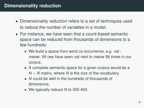
Dimensionality reduction
• Dimensionality reduction refers to a set of techniques usedto reduce the number of variables in a model.• For instance, we have seen that a count-based semantic
space can be reduced from thousands of dimensions to afew hundreds:• We build a space from word co-occurrence, e.g. cat -
meow: 56 (we have seen cat next to meow 56 times in ourcorpus.
• A complete semantic space for a given corpus would be aN × N matrix, where N is the size of the vocabulary.
• N could be well in the hundreds of thousands ofdimensions.
• We typically reduce N to 300-400.
4
From PCA to SVD
• We have seen that Principal Component Analysis (PCA) isused in the Partial Least Square Regression algorithm forsupervised learning.
• PCA is unsupervised in that it finds ‘the most important’dimensions in the data just by finding structure in that data.
• A possible way to find the principal components in PCA isto perform Singular Value Decomposition (SVD).
• Understanding SVD gives an insight into the nature of theprincipal components.
5
Singular Value Decomposition
• SVD is a matrix factorisation method which expresses amatrix in terms of three other matrices:
A = UΣV T
• U and V are orthogonal: they are matrices such that• UUT = UT U = I• VV T = V T V = I
I is the identity matrix: a matrix with 1s on the diagonal, 0s everywhere else.
• Σ is a diagonal matrix (only the diagonal entries arenon-zero).
6
Singular Value Decomposition over a semantic space
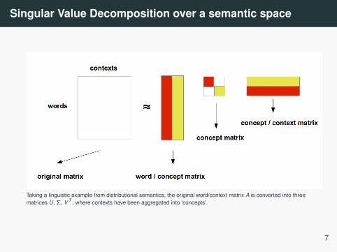
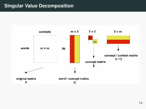
Taking a linguistic example from distributional semantics, the original word/context matrix A is converted into threematrices U, Σ, V T , where contexts have been aggregated into ‘concepts’.
7
The SVD derivation
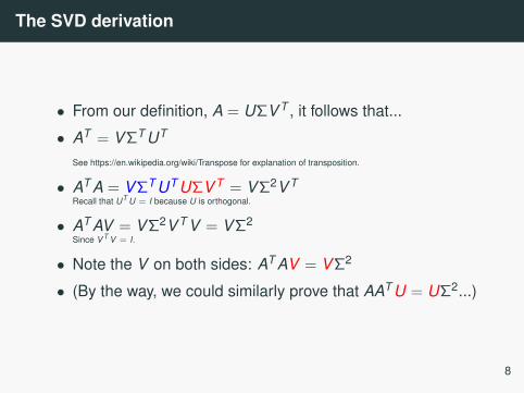
• From our definition, A = UΣV T , it follows that...
• AT = V ΣT UT
See https://en.wikipedia.org/wiki/Transpose for explanation of transposition.
• AT A = V ΣT UT UΣV T = V Σ2V TRecall that UT U = I because U is orthogonal.
• AT AV = V Σ2V T V = V Σ2Since V T V = I.
• Note the V on both sides: AT AV = V Σ2
• (By the way, we could similarly prove that AAT U = UΣ2...)
8
SVD and eigenvectors
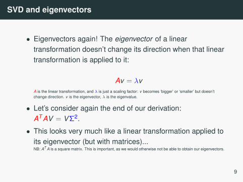
• Eigenvectors again! The eigenvector of a lineartransformation doesn’t change its direction when that lineartransformation is applied to it:
Av = λvA is the linear transformation, and λ is just a scaling factor: v becomes ‘bigger’ or ‘smaller’ but doesn’tchange direction. v is the eigenvector, λ is the eigenvalue.
• Let’s consider again the end of our derivation:AT AV = V Σ2.
• This looks very much like a linear transformation applied toits eigenvector (but with matrices)...NB: AT A is a square matrix. This is important, as we would otherwise not be able to obtain our eigenvectors.
9
SVD and eigenvectors
• The columns of V are the eigenvectors of AT A.(Similarly, the columns of U are the eigenvectors of AAT .)
• AT A computed over normalised data is the covariancematrix of A.See https://datascienceplus.com/understanding-the-covariance-matrix/.
• In other words, each column in V / U captures variancealong one of the (possibly rotated) dimensions of then-dimensional original data (see last week’s slides).
10
The singular values of SVD
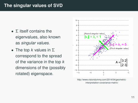
• Σ itself contains theeigenvalues, also knownas singular values.
• The top k values in Σ
correspond to the spreadof the variance in the top kdimensions of the (possiblyrotated) eigenspace.
http://www.visiondummy.com/2014/04/geometric-interpretation-covariance-matrix/
11
SVD at a glance
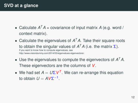
• Calculate AT A = covariance of input matrix A (e.g. word /context matrix).
• Calculate the eigenvalues of AT A. Take their square rootsto obtain the singular values of AT A (i.e. the matrix Σ).If you want to know how to compute eigenvalues, seehttp://www.visiondummy.com/2014/03/eigenvalues-eigenvectors/.
• Use the eigenvalues to compute the eigenvectors of AT A.These eigenvectors are the columns of V .
• We had set A = UΣV T . We can re-arrange this equationto obtain U = AV Σ−1.
12
Finally... dimensionality reduce!
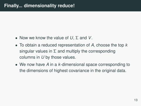
• Now we know the value of U, Σ and V .
• To obtain a reduced representation of A, choose the top ksingular values in Σ and multiply the correspondingcolumns in U by those values.
• We now have A in a k -dimensional space corresponding tothe dimensions of highest covariance in the original data.
13
Singular Value Decomposition
14
What semantic space?
• Singular Value Decomposition (LSA – Landauer andDumais, 1997). A new dimension might correspond to ageneralisation over several of the original dimensions (e.g.the dimensions for car and vehicle are collapsed into one).• + Very efficient (200-500 dimensions). Captures
generalisations in the data.• - SVD matrices are not straightforwardly interpretable.
Can you see why?
15
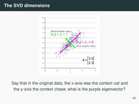
The SVD dimensions
Say that in the original data, the x-axis was the context cat andthe y-axis the context chase, what is the purple eigenvector?
16
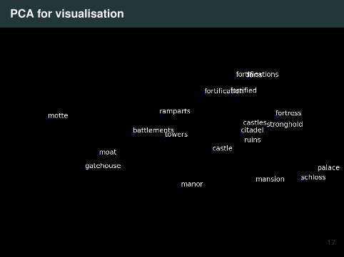
PCA for visualisation
17
Random indexing
18
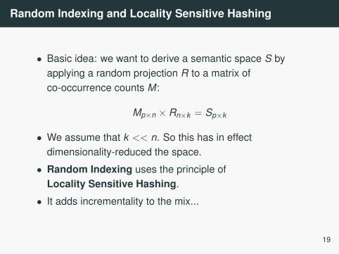
Random Indexing and Locality Sensitive Hashing
• Basic idea: we want to derive a semantic space S byapplying a random projection R to a matrix ofco-occurrence counts M:
Mp×n × Rn×k = Sp×k
• We assume that k << n. So this has in effectdimensionality-reduced the space.
• Random Indexing uses the principle ofLocality Sensitive Hashing.
• It adds incrementality to the mix...
19
Hashing: definition
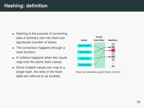
• Hashing is the process of convertingdata of arbitrary size into fixed sizesignatures (number of bytes).
• The conversion happens through ahash function.
• A collision happens when two inputsmap onto the same hash (value).
• Since multiple values can map to asingle hash, the slots in the hashtable are referred to as buckets.
https://en.wikipedia.org/wiki/Hash_function
20
Hash tables
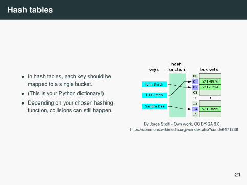
• In hash tables, each key should bemapped to a single bucket.
• (This is your Python dictionary!)
• Depending on your chosen hashingfunction, collisions can still happen.
By Jorge Stolfi - Own work, CC BY-SA 3.0,https://commons.wikimedia.org/w/index.php?curid=6471238
21
Hashing strings: an example
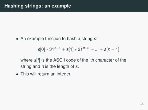
• An example function to hash a string s:
s[0] ∗ 31n−1 + s[1] ∗ 31n−2 + ...+ s[n − 1]
where s[i] is the ASCII code of the ith character of thestring and n is the length of s.
• This will return an integer.
22
Hashing strings: an example
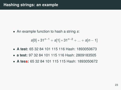
• An example function to hash a string s:
s[0] ∗ 31n−1 + s[1] ∗ 31n−2 + ...+ s[n − 1]
• A test: 65 32 84 101 115 116 Hash: 1893050673
• a test: 97 32 84 101 115 116 Hash: 2809183505
• A tess: 65 32 84 101 115 115 Hash: 1893050672
23
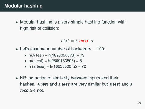
Modular hashing
• Modular hashing is a very simple hashing function withhigh risk of collision:
h(k) = k mod m
• Let’s assume a number of buckets m = 100:• h(A test) = h(1893050673) = 73• h(a test) = h(2809183505) = 5• h (a tess) = h(1893050672) = 72
• NB: no notion of similarity between inputs and theirhashes. A test and a tess are very similar but a test and atess are not.
24
Locality Sensitive Hashing
• In ‘conventional’ hashing, similarities between datapointsare not conserved.
• LSH is a way to produces hashes that can be comparedwith a similarity function.
• The hash function is a projection matrix defining a randomhyperplane. If the projected datapoint ~v falls on one side ofthe hyperplane, its hash h(~v) = +1, otherwise h(~v) = −1.
25
Locality Sensitive Hashing
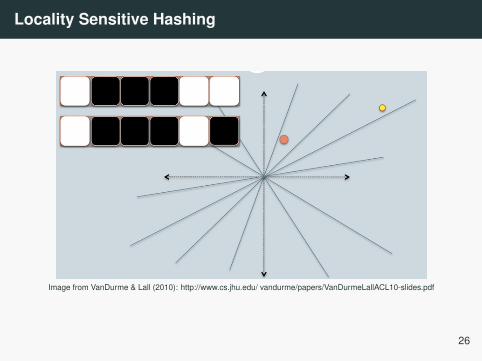
Image from VanDurme & Lall (2010): http://www.cs.jhu.edu/ vandurme/papers/VanDurmeLallACL10-slides.pdf
26
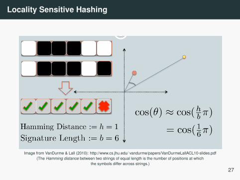
Locality Sensitive Hashing
Image from VanDurme & Lall (2010): http://www.cs.jhu.edu/ vandurme/papers/VanDurmeLallACL10-slides.pdf(The Hamming distance between two strings of equal length is the number of positions at which
the symbols differ across strings.)
27
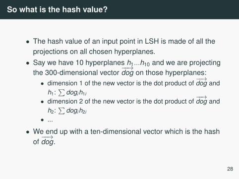
So what is the hash value?
• The hash value of an input point in LSH is made of all theprojections on all chosen hyperplanes.• Say we have 10 hyperplanes h1...h10 and we are projecting
the 300-dimensional vector−−→dog on those hyperplanes:
• dimension 1 of the new vector is the dot product of−−→dog and
h1:∑
dogih1i
• dimension 2 of the new vector is the dot product of−−→dog and
h2:∑
dogih2i
• ...
• We end up with a ten-dimensional vector which is the hashof−−→dog.
28
Interpretation of the LSH hash
• Each hyperplane is a discriminatory feature cutting throughthe data.
• Each point in space is expressed as a function of thosehyperplanes.
• We can think of them as new ‘dimensions’ relevant toexplaining the structure of the data.
• But how do we get the random matrix?
29
Gaussian random projections
• We want to perform Mp×n × Rn×k = Sp×k
• The random matrix R can be generated via a Gaussiandistribution.• For each row pi in the original matrix M:
• Generate a unit-length vector vi according to the Gaussiandistribution such that...
• vi is orthogonal to v1...i (to all other row vectors producedso far).
30
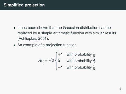
Simplified projection
• It has been shown that the Gaussian distribution can bereplaced by a simple arithmetic function with similar results(Achlioptas, 2001).
• An example of a projection function:
Ri,j =√
3
+1 with probability 1
6
0 with probability 23
−1 with probability 16
31
Random Indexing: incremental LSH
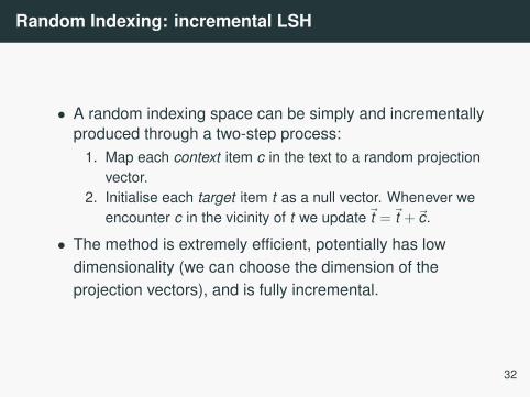
• A random indexing space can be simply and incrementallyproduced through a two-step process:
1. Map each context item c in the text to a random projectionvector.
2. Initialise each target item t as a null vector. Whenever weencounter c in the vicinity of t we update~t =~t + ~c.
• The method is extremely efficient, potentially has lowdimensionality (we can choose the dimension of theprojection vectors), and is fully incremental.
32
How is that LSH?
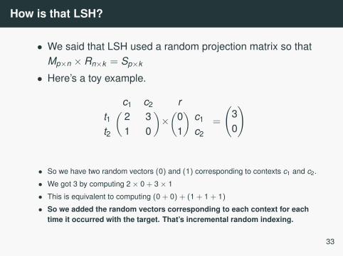
• We said that LSH used a random projection matrix so thatMp×n × Rn×k = Sp×k
• Here’s a toy example.
c1 c2( )t1 2 3t2 1 0
×
r( )0 c1
1 c2
=
(30
)
• So we have two random vectors (0) and (1) corresponding to contexts c1 and c2.
• We got 3 by computing 2× 0 + 3× 1
• This is equivalent to computing (0 + 0) + (1 + 1 + 1)
• So we added the random vectors corresponding to each context for eachtime it occurred with the target. That’s incremental random indexing.
33
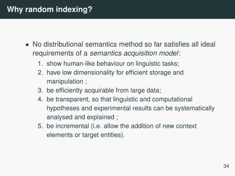
Why random indexing?
• No distributional semantics method so far satisfies all idealrequirements of a semantics acquisition model :
1. show human-like behaviour on linguistic tasks;2. have low dimensionality for efficient storage and
manipulation ;3. be efficiently acquirable from large data;4. be transparent, so that linguistic and computational
hypotheses and experimental results can be systematicallyanalysed and explained ;
5. be incremental (i.e. allow the addition of new contextelements or target entities).
34
Why random indexing?
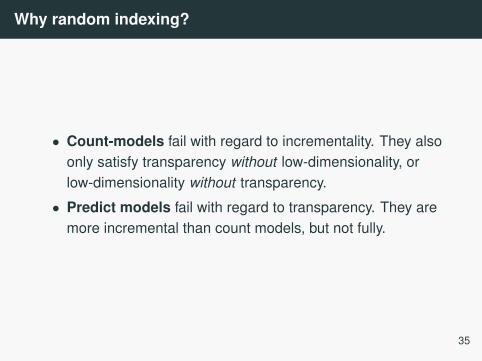
• Count-models fail with regard to incrementality. They alsoonly satisfy transparency without low-dimensionality, orlow-dimensionality without transparency.
• Predict models fail with regard to transparency. They aremore incremental than count models, but not fully.
35
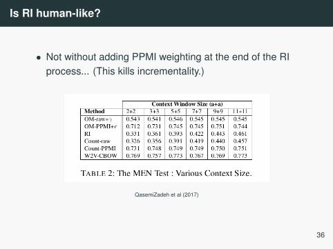
Is RI human-like?
• Not without adding PPMI weighting at the end of the RIprocess... (This kills incrementality.)
QasemiZadeh et al (2017)
36
Clustering
37
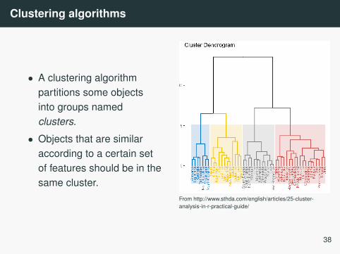
Clustering algorithms
• A clustering algorithmpartitions some objectsinto groups namedclusters.
• Objects that are similaraccording to a certain setof features should be in thesame cluster.
From http://www.sthda.com/english/articles/25-cluster-analysis-in-r-practical-guide/
38
Why clustering
• Example:1 we are translating from French to English, andwe know from some training data that:• Dimanche −→ on Sunday ;• Mercredi −→ on Wednesday ;
• What might be the correct preposition to translate Vendrediinto the English ___ Friday? (Given that we haven’t seen itin the training data.)
• We can assume that the days of the week form a semanticcluster, which behave in the same way syntactically. Here,clustering helps us generalise.
1Example from Manning & Schütze, Foundations of statistical language processing.
39
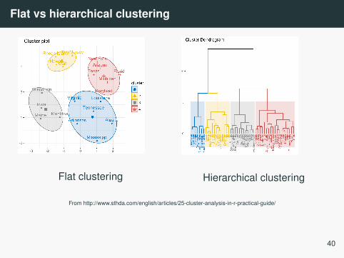
Flat vs hierarchical clustering
Flat clustering Hierarchical clustering
From http://www.sthda.com/english/articles/25-cluster-analysis-in-r-practical-guide/
40
Soft vs hard clustering
• In hard clustering, each object is assigned to only onecluster.
• In soft clustering, assignment can be to multiple clusters,or be probabilistic.
• In a probabilistic setup, each object has a probabilitydistribution over clusters. P(ck |xi) is the probability thatobject xi belongs to cluster ck .
• In a vector space, the degree of membership of an objectxi to each cluster can be defined by the similarity of xi tosome representative point in the cluster.
41
Centroids and medoids
• The centroid or center of gravity of a cluster c is theaverage of its N members:
µk =1N
∑x∈ck
x
• The medoid of a cluster c is a prototypical member of thatcluster (its average dissimilarity to all other objects in c isminimal):
xmedoid = argminy∈{x1,x2,··· ,xn}
n∑i=1
d(y , xi)
42
Hierarchical clustering: bottom-up
• Bottom-up agglomerative clustering is a form ofhierarchical clustering.• Let’s have n datapoints x1...xn. The algorithm functions as
follows:• Start with one cluster per datapoint: ci := {xi}.• Determine which two clusters are the most similar and
merge them.• Repeat until we are left with only one cluster C = {x1...xn}.
43
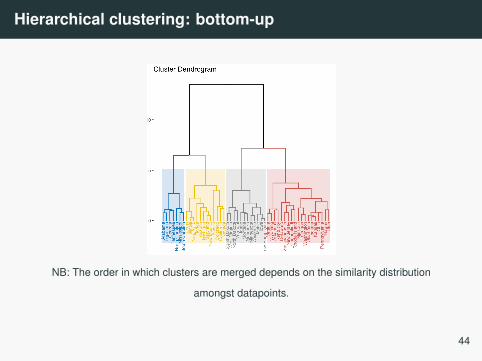
Hierarchical clustering: bottom-up
NB: The order in which clusters are merged depends on the similarity distribution
amongst datapoints.
44
Hierarchical clustering: top-down
• Top-down divising clustering is the pendent ofagglomerative clustering.• Let’s have n datapoints again: x1...xn. The algorithm relies
on a coherence and a split function:• Start with a single cluster C = {x1...xn}• Determine the least coherent cluster and split it into two
new clusters.• Repeat until we have one cluster per datapoint: ci := {xi}.
45
Coherence
• Coherence is a measure of the pairwise similarity of a setof objects.
• A typical coherence function:
Coh(x1...n) = mean{Sim(xi , xj), ij ∈ 1...n, i < j}
• E.g. coherence may be used to calculate the consistencyof topics in topic modelling.
46
Similarity functions for clustering
• Single link: similarity of two most similar objects acrossclusters.
• Complete link: similarity of two least similar objectsacross clusters.
• Group-average: average similarity between objects.(Here, the average is over all pairs, within and acrossclusters.)
47
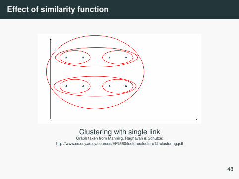
Effect of similarity function
Clustering with single linkGraph taken from Manning, Raghavan & Schütze:
http://www.cs.ucy.ac.cy/courses/EPL660/lectures/lecture12-clustering.pdf
48
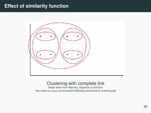
Effect of similarity function
Clustering with complete linkGraph taken from Manning, Raghavan & Schütze:
http://www.cs.ucy.ac.cy/courses/EPL660/lectures/lecture12-clustering.pdf
49
K-means clustering
• K-means is the main flat clustering algorithm.
• Goal in K-means: minimise the residual sum of squares(RSS) of objects to their cluster centroids:
RSSk =∑x∈ck
|x − µk |2
• The intuition behind using RSS is that good clusters shouldhave a) small intra-cluster distances; b) large inter-clusterdistances.
50
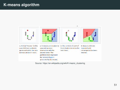
K-means algorithm
Source: https://en.wikipedia.org/wiki/K-means_clustering
51
Convergence
• Convergence happens when the RSS will not decreaseanymore.
• It can be shown that K-means will converge to a localminimum, but not necessarily a global minimum.
• Results will vary depending on seed selection.
52
Initialisation
• Various heuristics to ensure good clustering:• exclude outliers from seed sets;• try multiple intialisations and retain the one with lowest
RSS;• obtain seeds from another method (e.g. first do hierarchical
clustering).
53
Number of clusters
• The number of clusters K is predefined.
• The ideal K will minimise variance within each cluster aswell as minimise the number of clusters.• There are various approaches to finding K . Examples that
use techniques we have already learnt:• cross-validation;• PCA.
54
Number of clusters
• Cross-validation: split the data into random folds andcluster with some k on one fold. Repeat on the other folds.If points consistently get assigned to the same clusters (ifmembership is roughly the same across folds) then k isprobably right.
• PCA: there is no systematic relation between principalcomponents and clusters, but heuristically checking howmany components account for most of the data’s variancecan give a fair idea of the ideal cluster number.
55
Evaluation of clustering
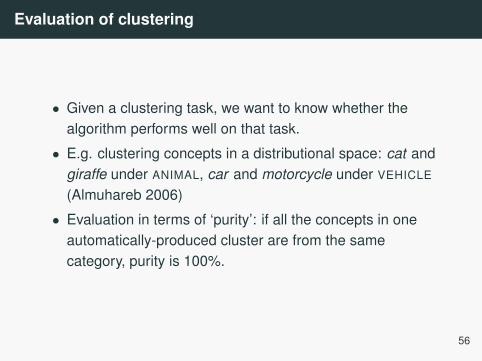
• Given a clustering task, we want to know whether thealgorithm performs well on that task.
• E.g. clustering concepts in a distributional space: cat andgiraffe under ANIMAL, car and motorcycle under VEHICLE
(Almuhareb 2006)
• Evaluation in terms of ‘purity’: if all the concepts in oneautomatically-produced cluster are from the samecategory, purity is 100%.
56
Purity measure
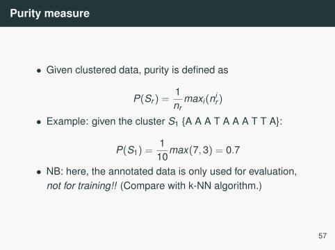
• Given clustered data, purity is defined as
P(Sr ) =1nr
maxi(nir )
• Example: given the cluster S1 {A A A T A A A T T A}:
P(S1) =1
10max(7,3) = 0.7
• NB: here, the annotated data is only used for evaluation,not for training!! (Compare with k-NN algorithm.)
57

Clustering in real life
58
Dimensionality reduction and primitives
59
So what are those dimensions?
• Dimensionality-reduced spaces are not very interpretable.
• A count-based semantic space has dimensions labelledwith words (or any other linguistic constituent). Afterreduction, the dimensions are unlabelled.
• The following is taken from Boleda & Erk (2015):Distributional Semantic Features as Semantic Primitives -or not.
60
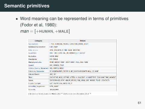
Semantic primitives
• Word meaning can be represented in terms of primitives(Fodor et al, 1980):man = [+HUMAN,+MALE]
61
Semantic primitives: why
• To capture aspects of the real world (see again differencebetween word usage and extension).
• To formalise commonalities between near-synonymousexpressions:Kim gave a book to Sandy ≈ Sandy received a book fromKim.
• To do inference: John is a human follows from John is aman.
62
Problems with primitives
• Primitives are ill-defined. They need to be extra-linguistic inorder to avoid circularity.E.g. if BACHELOR is defined as = [+MAN,+UNMARRIED],what are MAN and UNMARRIED?
• But sensory-motor properties are probably not fit to explainthe semantic blocks of language (at least alone).E.g. GRANDMOTHER in my cat’s grandmother.
63
Problems with primitives
• If primitives were real, they should be detectable inpsycholinguistic experiments. For instance, the effect ofnegation should be noticeable in processing times:BACHELOR = [+MAN,−MARRIED]
But no such effect has been found.
• Meaning nuances are lost in primitives:KILL ≈ [+CAUSE,−ALIVE]
(There are many causes for not being alive which do notinvolve killing.)
64
Relation to distributional semantic spaces
• Might the features of a distributional space replace thenotion of primitive?• Only a reduced number of dimensions is needed (≈ 300
seems to be a magic number).• They can include both linguistic and extra-linguistic
information.• Distributional representations do correlate with measurable
human judgements.• They are made of continuous values, which in combination
can express very graded meanings.
65
Inference
• Does distributional semantics satisfy the requirement thatprimitives should give us inference?• To some extent...
• Hyponymy can be learnt (e.g. Roller et al, 2014).• Some entailment relations can be learnt (e.g. Baroni et al
2012 on quantifiers.)
• But: distributional inference is soft, non-logical inference.
66
Dimensions as semantic primes?
• It may be that reduced distributional matrices captureimportant commonalities across word meanings and canbe seen as an alternative to primitives.
• But we remain unable to tell what those primitives stand for.
• (We can hack it, though...)
67