SVD and PCA COS 323. Dimensionality Reduction Map points in high-dimensional space to lower number of dimensionsMap points in high-dimensional space to

SVD and PCASVD and PCA

COS 323COS 323

Dimensionality ReductionDimensionality Reduction

• Map points in high-dimensional space toMap points in high-dimensional space tolower number of dimensionslower number of dimensions

• Preserve structure: pairwise distances, Preserve structure: pairwise distances, etc.etc.

• Useful for further processing:Useful for further processing:– Less computation, fewer parametersLess computation, fewer parameters

– Easier to understand, visualizeEasier to understand, visualize

PCAPCA

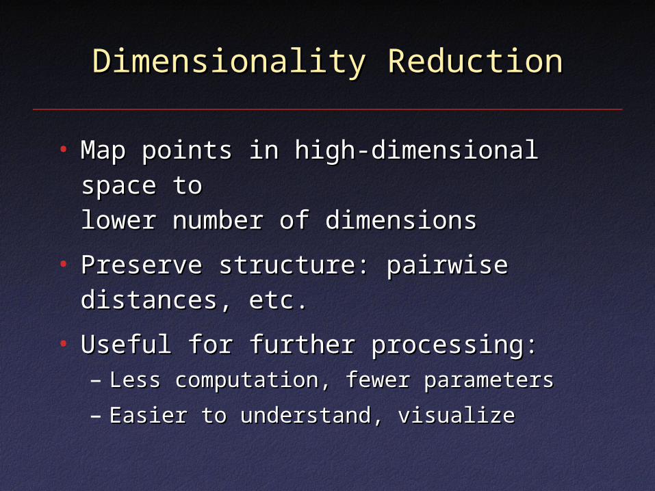
• Principal Components Analysis (PCA): Principal Components Analysis (PCA): approximating a high-dimensional data approximating a high-dimensional data setsetwith a lower-dimensional linear with a lower-dimensional linear subspacesubspace

Original axesOriginal axes

****

******

**** **

**

********

**

**

****** **

**** ******

Data pointsData points

First principal componentFirst principal componentSecond principal componentSecond principal component

SVD and PCASVD and PCA

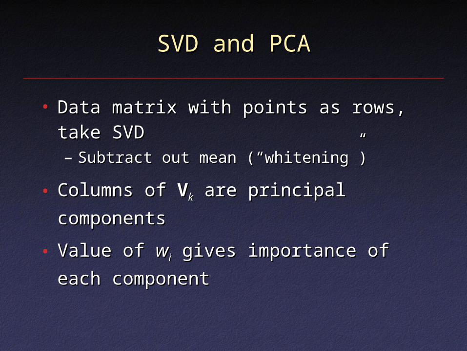
• Data matrix with points as rows, take Data matrix with points as rows, take SVDSVD– Subtract out mean (“whitening”)Subtract out mean (“whitening”)

• Columns of Columns of VVkk are principal components are principal components

• Value of Value of wwii gives importance of each gives importance of each

componentcomponent

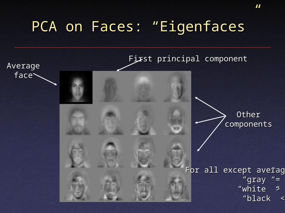
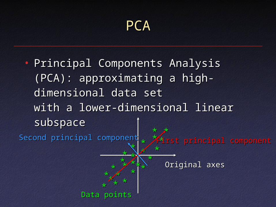
PCA on Faces: “Eigenfaces”PCA on Faces: “Eigenfaces”

AverageAveragefaceface

First principal componentFirst principal component

OtherOthercomponentscomponents

For all except average,For all except average,“gray” = 0,“gray” = 0,

“white” > 0,“white” > 0,““black” < 0black” < 0

Uses of PCAUses of PCA

• Compression: each new image can be Compression: each new image can be approximated by projection onto first approximated by projection onto first few principal componentsfew principal components

• Recognition: for a new image, project Recognition: for a new image, project onto first few principal components, onto first few principal components, match feature vectorsmatch feature vectors

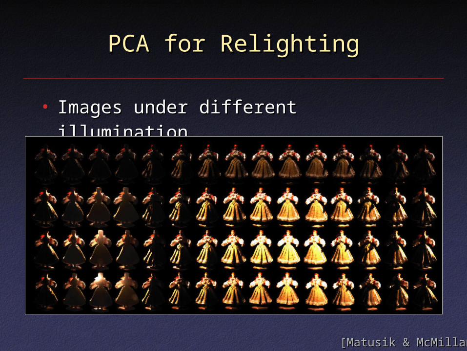
PCA for RelightingPCA for Relighting

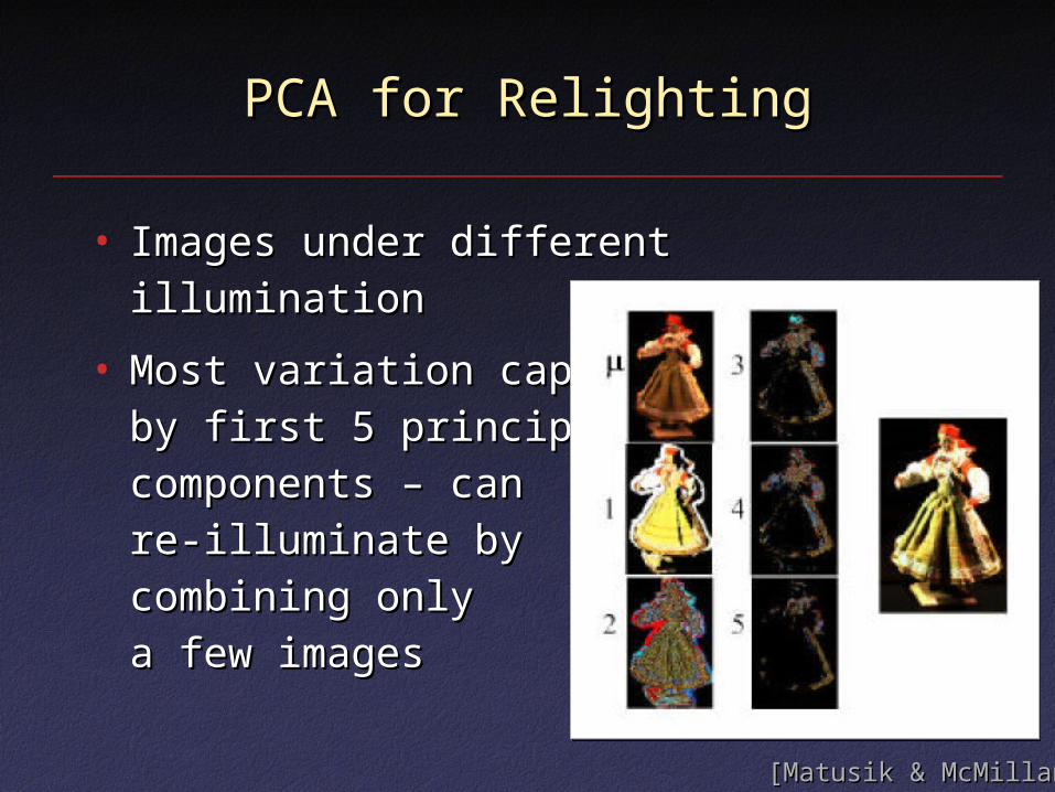
• Images under different illuminationImages under different illumination

[Matusik & McMillan][Matusik & McMillan]

PCA for RelightingPCA for Relighting

• Images under different illuminationImages under different illumination

• Most variation capturedMost variation capturedby first 5 principalby first 5 principalcomponents – cancomponents – canre-illuminate byre-illuminate bycombining onlycombining onlya few imagesa few images

[Matusik & McMillan][Matusik & McMillan]

PCA for DNA MicroarraysPCA for DNA Microarrays

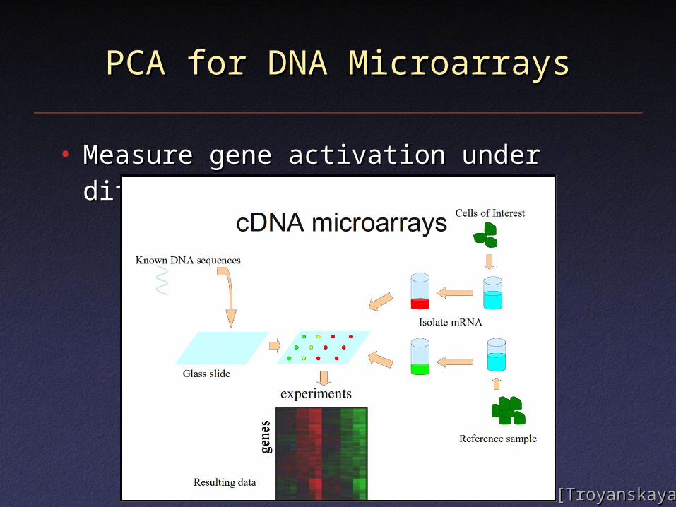
• Measure gene activation under different Measure gene activation under different conditionsconditions

[Troyanskaya][Troyanskaya]


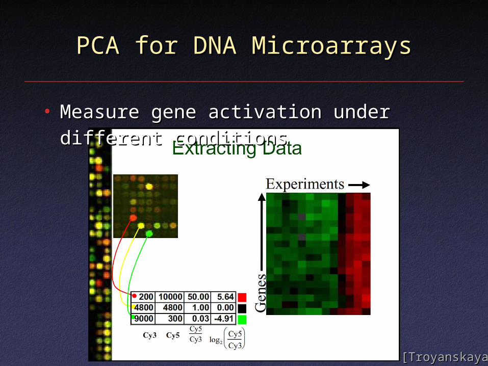
• Measure gene activation under different Measure gene activation under different conditionsconditions

[Troyanskaya][Troyanskaya]


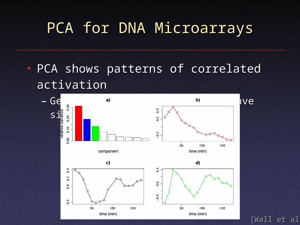
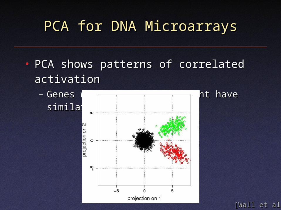
• PCA shows patterns of correlated PCA shows patterns of correlated activationactivation– Genes with same pattern might have similar Genes with same pattern might have similar

functionfunction

[Wall et al.][Wall et al.]


• PCA shows patterns of correlated PCA shows patterns of correlated activationactivation– Genes with same pattern might have similar Genes with same pattern might have similar

functionfunction

[Wall et al.][Wall et al.]

Multidimensional ScalingMultidimensional Scaling

• In some experiments, can only measure In some experiments, can only measure similarity or dissimilaritysimilarity or dissimilarity– e.g., is response to stimuli similar or e.g., is response to stimuli similar or

different?different?

– Frequent in psychophysical experiments,Frequent in psychophysical experiments,preference surveys, etc.preference surveys, etc.

• Want to recover absolute positions inWant to recover absolute positions ink-dimensional spacek-dimensional space


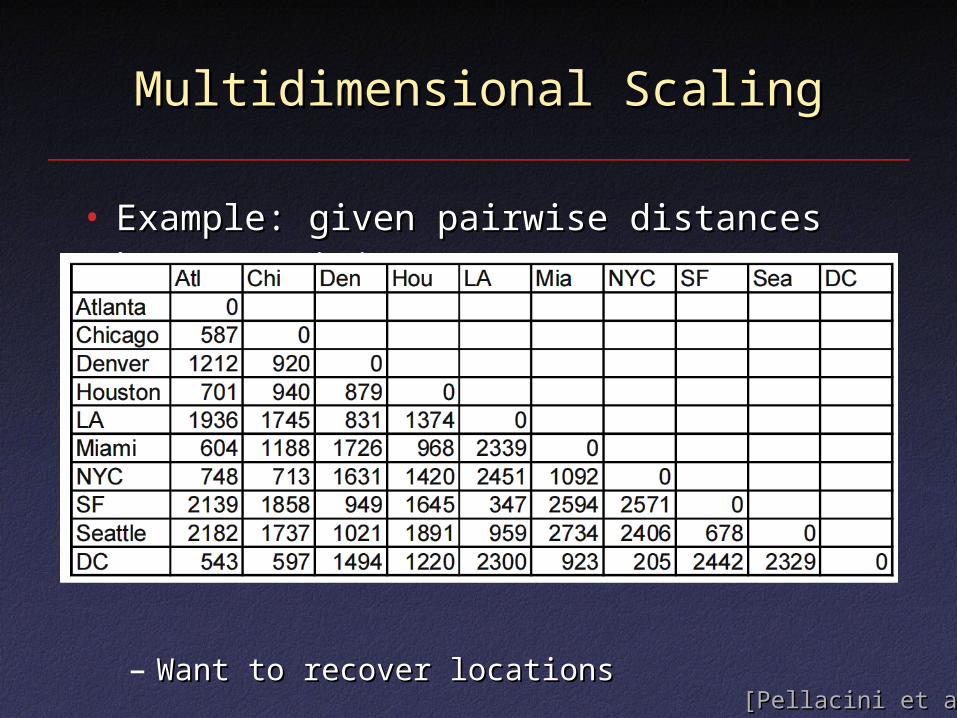
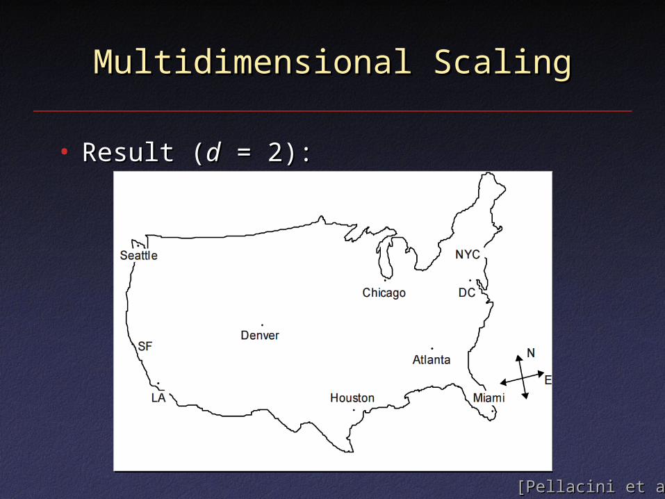
• Example: given pairwise distances Example: given pairwise distances between citiesbetween cities

– Want to recover locationsWant to recover locations [Pellacini et al.][Pellacini et al.]

Euclidean MDSEuclidean MDS

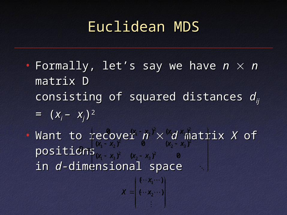
• Formally, let’s say we have Formally, let’s say we have nn nn matrix matrix DDconsisting of squared distances consisting of squared distances ddijij = ( = (xxi i – –

xxjj))22

• Want to recover Want to recover nn dd matrix matrix XX of of positionspositionsin in dd-dimensional space-dimensional space

)(

)(

0)()(

)(0)(

)()(0

2

1

232

231

232

221

231

221

x

x

X

xxxx

xxxx

xxxx

D

)(

)(

0)()(

)(0)(

)()(0

2

1

232

231

232

221

231

221

x

x

X

xxxx

xxxx

xxxx

D


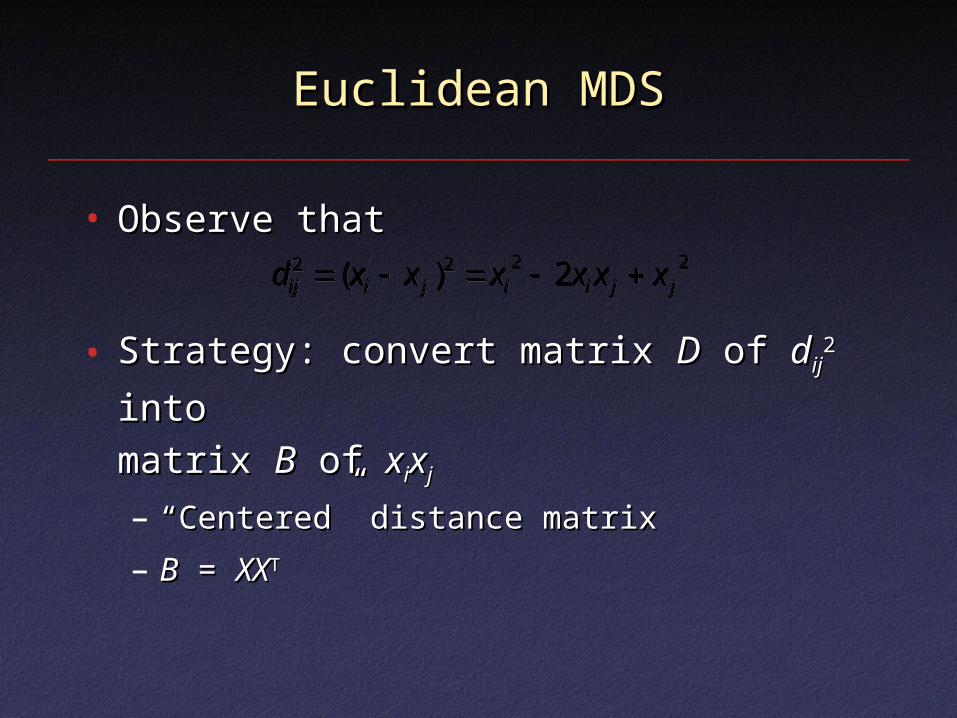
• Observe thatObserve that

• Strategy: convert matrix Strategy: convert matrix DD of of ddijij22 into into

matrix matrix BB of of xxiixxjj

– ““Centered” distance matrixCentered” distance matrix

– BB = = XXXXTT

2222 2)( jjiijiij xxxxxxd 2222 2)( jjiijiij xxxxxxd


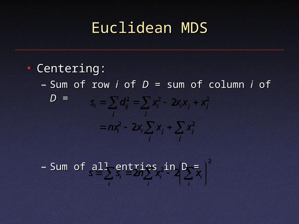
• Centering:Centering:– Sum of row Sum of row ii of of DD = sum of column = sum of column ii of of DD = =

– Sum of all entries in D =Sum of all entries in D =

jj

jjii

jjij j

iiji

xxxnx

xxxxds

22

222

2

2

jj

jjii

jjij j

iiji

xxxnx

xxxxds

22

222

2

2

2

2 22

ii

ii

ii xxnss

2

2 22

ii

ii

ii xxnss


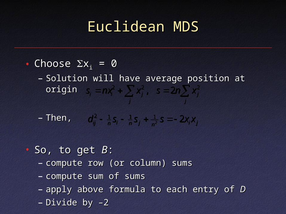
• Choose Choose xxii = 0 = 0– Solution will have average position at originSolution will have average position at origin

– Then,Then,

• So, to get So, to get BB::– compute row (or column) sumscompute row (or column) sums

– compute sum of sumscompute sum of sums

– apply above formula to each entry of apply above formula to each entry of DD

– Divide by –2Divide by –2

j

jj

jii xnsxnxs 222 2, j

jj

jii xnsxnxs 222 2,

jinjninij xxsssd 221112 jinjninij xxsssd 221112


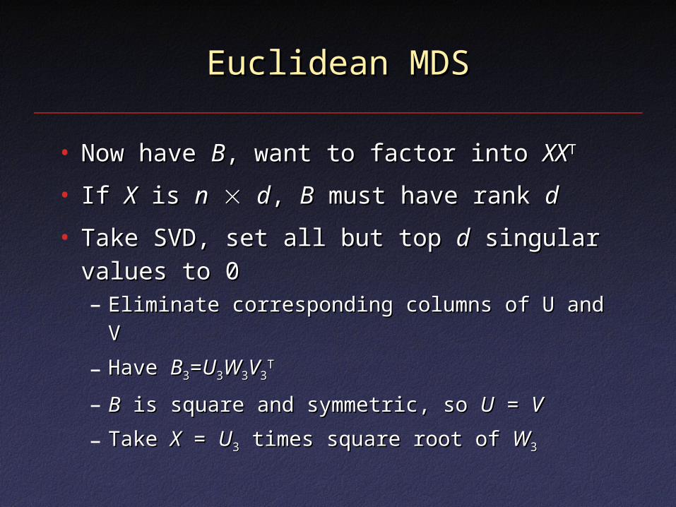
• Now have Now have BB, want to factor into , want to factor into XXXXTT

• If If XX is is nn dd, , BB must have rank must have rank dd

• Take SVD, set all but top Take SVD, set all but top dd singular singular values to 0values to 0– Eliminate corresponding columns of U and VEliminate corresponding columns of U and V

– Have Have BB33==UU33WW33VV33TT

– BB is square and symmetric, so is square and symmetric, so UU = = VV

– Take Take XX = = UU33 times square root of times square root of WW33


• Result (Result (dd = 2): = 2):

[Pellacini et al.][Pellacini et al.]


• Caveat: actual axes, center not necessarilyCaveat: actual axes, center not necessarilywhat you want (can’t recover them!)what you want (can’t recover them!)

• This is “classical” or “Euclidean” MDS This is “classical” or “Euclidean” MDS [Torgerson [Torgerson

52]52]

– Distance matrix assumed to be actual Euclidean Distance matrix assumed to be actual Euclidean distancedistance

• More sophisticated versions availableMore sophisticated versions available– ““Non-metric MDS”: not Euclidean distance,Non-metric MDS”: not Euclidean distance,

sometimes just sometimes just inequalitiesinequalities

– ““Weighted MDS”: account for observer biasWeighted MDS”: account for observer bias

ComputationComputation

• SVD very closely related to SVD very closely related to eigenvalue/vector computationeigenvalue/vector computation– Eigenvectors/values of AEigenvectors/values of ATTAA

– In practice, similar class of methods, butIn practice, similar class of methods, butoperate on A directlyoperate on A directly

Methods for Eigenvalue Methods for Eigenvalue ComputationComputation

• Simplest: Simplest: power methodpower method– Begin with arbitrary vector xBegin with arbitrary vector x00

– Compute xCompute xi+1i+1=Ax=Axii

– NormalizeNormalize

– IterateIterate

• Converges to eigenvector with Converges to eigenvector with maximum eigenvalue!maximum eigenvalue!

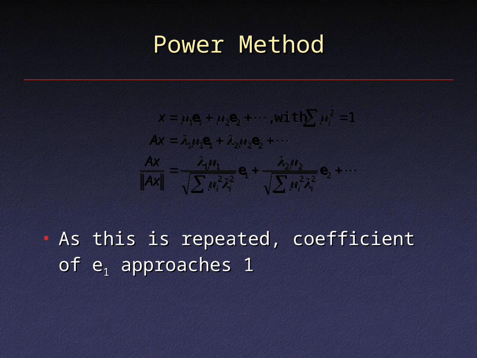
Power MethodPower Method

• As this is repeated, coefficient of eAs this is repeated, coefficient of e11

approaches 1approaches 1

222

22122

11

222111

22211 1with,

ee

ee

ee

iiii

i

Ax

Ax

Ax

x

222

22122

11

222111

22211 1with,

ee

ee

ee

iiii

i

Ax

Ax

Ax

x

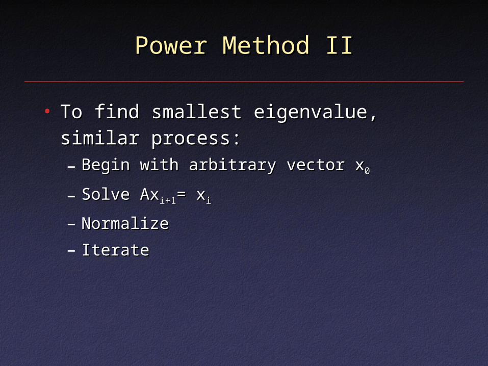
Power Method IIPower Method II

• To find smallest eigenvalue, similar To find smallest eigenvalue, similar process:process:– Begin with arbitrary vector xBegin with arbitrary vector x00

– Solve AxSolve Axi+1i+1= x= xii

– NormalizeNormalize

– IterateIterate

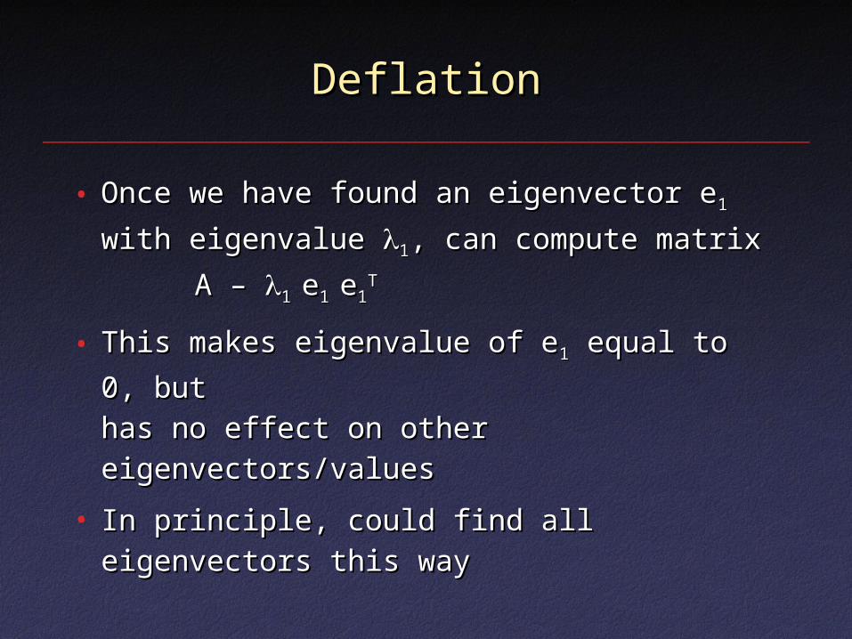
DeflationDeflation

• Once we have found an eigenvector eOnce we have found an eigenvector e11

with eigenvalue with eigenvalue 11, can compute matrix, can compute matrix

A – A – 1 1 ee1 1 ee11TT

• This makes eigenvalue of eThis makes eigenvalue of e11 equal to 0, equal to 0,

butbuthas no effect on other eigenvectors/valueshas no effect on other eigenvectors/values

• In principle, could find all eigenvectors this In principle, could find all eigenvectors this wayway

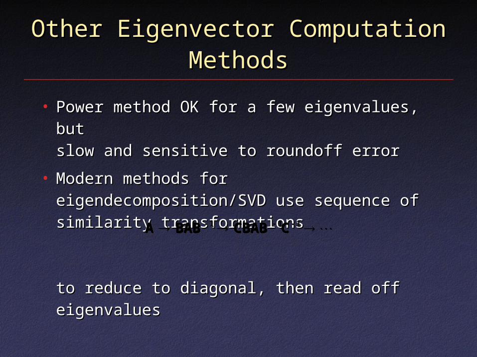
Other Eigenvector Computation Other Eigenvector Computation MethodsMethods

• Power method OK for a few eigenvalues, butPower method OK for a few eigenvalues, butslow and sensitive to roundoff errorslow and sensitive to roundoff error

• Modern methods for Modern methods for eigendecomposition/SVD use sequence of eigendecomposition/SVD use sequence of similarity transformationssimilarity transformations

to reduce to diagonal, then read off to reduce to diagonal, then read off eigenvalueseigenvalues

111 CCBABBABA 111 CCBABBABA

Documents

SVD and PCA COS 323. Dimensionality Reduction Map points in high-dimensional space to lower number of dimensionsMap points in high-dimensional space to