Embed Size (px)
Citation preview
A path-integral formalism of DNA looping
probability
Ludovica Cotta-Ramusino
January 7, 2008
Abstract
In this thesis we describe a path integral formalism to evaluate approximations to
the probability density function for the location and orientation of one end of a
continuum polymer chain at thermodynamic equilibrium with a heat bath. We
concentrate on those systems for which the associated energy density is at most
quadratic in its variables. Our main motivation is to exploit continuum elastic rod
models for the approximate computation of DNA looping probabilities.
We first re-derive, for a polymer chain system, an expression for the second
order correction term due to quadratic fluctuations about a unique minimal energy
configuration. The result, originally stated for a quantum mechanical system by G.
Papadopoulos (1975), relies on an elegant algebraic argument that carries over to the
real-valued path integrals of interest here. The conclusion is that the appropriate
expression can be evaluated in terms of the energy of the minimizer and the inverse
square root of the determinant of a matrix satisfying a certain non-linear system of
differential equations.
We then construct a change of variables, which establishes a mapping between
the solutions of the aforementioned non-linear Papadopoulos equations and a matrix
satisfying an initial value problem for the classic linear system of Jacobi equations
associated with the second variation of the energy functional. This conclusion is
trivial if no cross-term is present in the second variation, but ceases to be so oth-
erwise. Cross-terms are always present in the application of rod models to DNA.
We therefore can conclude that the second order fluctuation correction term to the
probability density function for a chain is always given by the inverse square root
of the determinant of a matrix of solutions to the Jacobi equations. We believe this
conclusion to be original for the real-valued case when the second-variation involves
cross-terms. Similar results are known for quantum mechanical systems, and, in
this context, a connection between the so called Van-Hove-Morette determinant,
which involves partial derivatives of the classical action with respect to the bound-
ary values of the configuration variable, and the Jacobi determinant have also been
ii
established.
We next apply the formula described above to the specific context of rods, for
which the configuration space is that of framed curves, or curves in R3×SO(3). An
immediate application of our theory is possible if the rod model encompasses bend,
twist, stretch and shear. However the constrained case, where the rod is considered
to be inextensible and unshearable, is more standard in polymer physics. In this last
case, our results are more delicate as the Lagrangian description breaks down, and
the Hamiltonian formulation must be invoked. It is known that the unconstrained
local minimizers approach constrained minimizers as the coefficients in the shear
and extension terms of the energy are sent to infinity. Here we observe that the
Hamiltonian form of the unconstrained Jacobi system similarly has a limit, so that
the fluctuation correction in the path integral can still be expressed as the square root
of the determinant of a matrix solution of a set of Jacobi equations appropriate to the
constrained problem. As in reality DNA or biological macromolecules are certainly
at least slightly shearable and extensible, the limit of the fluctuation correction is
undoubtedly physically appropriate.
The above theory provides a computationally highly tractable approach to the
estimation of the appropriate probability density functions. For application to
sequence-dependent models of DNA the associated systems of equations has non-
constant coefficients, which is of little consequence for a numerical treatment, but
precludes the possibility of finding closed form expressions. On the other hand the
theory also applies to simplified homogeneous models. Accordingly, we conclude by
applying our approach in a completely analytic and closed-form way to the compu-
tation of the approximate probability density function for a uniform, non-isotropic,
intrinsically straight and untwisted rod to form a circular loop.
Key-words: DNA looping and cyclization, path integrals.
iii
Riassunto
In questa tesi descriviamo un formalismo in termini di integrali di cammino atto
a determinare la densita di probabilita per un polimero semiflessibile, in equilibrio
termodinamico con una bagno termico, di avere un’estremita fissata nello spazio per
posizione ed orientamento. La nostra attenzione e principalmente rivolta a sistemi
per cui l’energia associata sia quadratica nelle relative variabili. L’obiettivo e la
motivazione generale consistono nell’utilizzare modelli di tipo corda elastica continua
per il calcolo approssimato della probabilita che un determinato frammento di DNA
formi un loop aperto o chiuso.
In prima istanza, seguendo l’approcio utilizzato da G.Papadopoulos (1975), ri-
caviamo un espressione per il contributo al secondo ordine dovuto alle fluttuazioni
armoniche attorno alla configurazione di minima energia. La conclusione, origina-
riamente tratta per un sistema quantistico, e che, al secondo ordine, la densita di
probabilita puo essere valutata come prodotto di due termini: il primo dipende es-
clusivamente dall’energia della configurazione di minima energia, mentre il secondo
e dato dall’inverso della radice quadrata del determinante di una matrice che sod-
disfa un’equazione differenziale non lineare. L’argomentazione seguita, di natura
algebrica, si adatta con naturalita al caso di interesse di integrali di cammino reali.
In seguito, costruiamo un cambiamento di variabile non lineare che permetta di
associare soluzioni della sopra menzionata equazione differenziale non lineare con
una matrice di soluzioni dell’equazione di Jacobi, e appropriate condizioni iniziali,
per la variazione seconda del funzionale di energia associato al sistema. Tale as-
sociazione risulta banale nel caso in cui non vi siano termini misti nella variazione
seconda, in quanto i due sistemi di equazioni coincidono. Nel caso invece in cui
siano presenti termini misti, come per modelli di corda elastica per il DNA, alcuna
relazione appare evidente. Concludiamo dunque che nella densita di probabilita
il contributo delle fluttuazioni quadratiche attorno alla configurazione di minimo e
sempre associato ad una matrice di soluzioni dell’equazione di Jacobi. Riteniamo che
questa conclusione sia originale nel caso di integrali di cammino reali per un’energia
iv
la cui variazione seconda contenga termini misti. Risultati analoghi sono noti in
contesti di meccanica quantistica dove anche una connessione tra il determinante
funzionali di Van-Hove-Morette, che coinvolge derivate parziali dell’azione valutata
sul cammino classico rispetto a valori specifici della configurazione iniziale o finale,
e il determinante della matrice di Jacobi.
Successivamente applichiamo la teoria ricavata al caso di una corda elastica lin-
eare in cui lo spazio delle configurazioni sia quello delle curve orientate. Un’applicazione
immediata e possibile qualora la corda possa essere sottoposta a piegamento, tor-
sione, allungamento e deformazioni della sezione in due direzioni ortogonali. Tut-
tavia nel caso piu comunemente trattato in letteratura in cui la corda non possa
ne essere allungata o compressa ne subire deformazioni della sezione, la descrizione
Lagrangiana da noi utilizzata non e piu valida e una descrizione Hamiltoniana deve
essere adottata. E ben noto che minimi locali di una corda non vincolata, tendano
ai minimi di una corda vincolata al tendere all’infinito delle rigidita associate alle
deformazioni che vengono precluse. Tuttavia, qui notiamo che anche la versione
Hamiltoniana dell’equazioni di Jacobi ha un limite, cosı che il termine di correzione
dovuto alla fluttuazioni quadratiche possa essere ancora espresso in funzione della
matrice di soluzioni dell’equazione di Jacobi opportuna. Poiche in realta il DNA o
altre macromolecole biologiche sono certamente estensibili e deformabili, per quanto
in maniera non sostanziale, l’approcio al limite seguito e senza dubbio almeno fisi-
camente quello corretto.
La teoria ricavata puo essere applicata a differenti situazioni. In particolare in
situazioni in cui la corda elastica venga utilizzata per descrivere frammenti di DNA
non omogenei e in cui l’interesse sia di evidenziare le proprieta meccaniche in fun-
zione della sequenza di basi. In questo caso, le equazioni di Jacobi sono a coefficienti
non costanti, e una trattazione di tipo numerico, per quanto di facile implemen-
tazione, si rende necessaria. Al contrario modelli omogenei possono essere risolti
analiticamente. Congruamente, concludiamo la tesi fornendo espressioni analitiche
per il calcolo approssimato della densita di probabilita per una corda uniforme, non
isotropa, intrinsicamente dritta e senza twist di formare una configurazione circolare.
Parole chiave: formazione di loop di DNA, integrali di cammino.
v
Acknowledgments
I wish to thank my supervisor Prof. John H. Maddocks, for proposing this topic of
research to me and giving me the opportunity to pursue it within his group, offering
continuous advice and support. I am looking forward to our future collaboration.
I also particularly thank Prof. Oliver Penrose, who after early discussions of the
problem, wrote a set of notes describing one approach to the cyclization problem,
that eventually lead us to the formalism adopted here. I greatly acknowledge Prof.
George Papadopoulos for discussions on his paper from which this work also has
started off.
I thank the committee: Prof. Philippe Choquard, Prof. Bertrand Duplantier,
Prof. Charles Pfister and Prof. Tudor Ratiu for carefully reading the thesis, spotting
errors and suggesting improvements.
I thank all present and former collegues at LCVMM. Particularly: Carine Tschanz
for always helping me with a smile; Philippe Caussignac, Mathias Carlen and Hen-
ryk Gerlach for their help in several computer emergencies; Angelo Rosa and Arnaud
Amzallag for scientific discussions.
I thank Prof. Douglas Arnold, Director of IMA at the University of Minneapolis,
for the hospitality in these last months.
I thank Daniela Silvano and Giovanni Costantini for their precious friendship and
for sharing the ups and downs of our PhDs until the very last day; Francesco Esposito
for his inspiring passion for mathematics and for helping me with the graphs; Chiara
Casella and Mauro Donega for being so close to family for me. I thank Valentina
Troncale, Davide Sarchi and Maria-Carola Colombo for many discussions on research
and life; Marc-Olivier Boldi and Lionel Pournin for the mornings and evenings in
our beautiful apartment in Lausanne.
Last, but not least, I thank my family, Paolo, Mariola, Cecilia and Giovanni.
Flic, we are all waiting for you! And my friends back in Italy and elsewhere. Giulia,
Laura, Silvia, Francesco, Davide, Amsicora, Blue, Jose, Marco, Adriana, Tommaso.
Without them, simply, I would not be.
vi
Contents
Introduction 1
1 Continuum elastic rod models for DNA 7
1.1 Special Cosserat model . . . . . . . . . . . . . . . . . . . . . . . . . . 7
1.1.1 Kinematics . . . . . . . . . . . . . . . . . . . . . . . . . . . . 9
1.1.2 Force and balance laws . . . . . . . . . . . . . . . . . . . . . . 10
1.1.3 Constitutive relations . . . . . . . . . . . . . . . . . . . . . . . 10
1.2 The variational formulation . . . . . . . . . . . . . . . . . . . . . . . 11
1.2.1 First order variation . . . . . . . . . . . . . . . . . . . . . . . 12
1.2.2 Second order variation . . . . . . . . . . . . . . . . . . . . . . 14
1.3 Constrained systems . . . . . . . . . . . . . . . . . . . . . . . . . . . 16
1.3.1 First order variation . . . . . . . . . . . . . . . . . . . . . . . 17
1.3.2 Second order variation . . . . . . . . . . . . . . . . . . . . . . 18
1.4 Conclusions and summary . . . . . . . . . . . . . . . . . . . . . . . . 19
2 General quadratic energy densities: a path integral approach for
computing conditional probabilities 21
2.1 Statement of the problem . . . . . . . . . . . . . . . . . . . . . . . . 22
2.2 Approximation about the minimal energy configuration . . . . . . . . 25
2.2.1 Recovering Papadopoulos equations . . . . . . . . . . . . . . . 27
2.3 A formula for the second order correction . . . . . . . . . . . . . . . . 35
2.3.1 Relating Papadopoulos to Jacobi . . . . . . . . . . . . . . . . 35
2.3.2 Riccati matrix equations . . . . . . . . . . . . . . . . . . . . . 39
2.3.3 The final formula . . . . . . . . . . . . . . . . . . . . . . . . . 41
2.4 Conclusions and discussion . . . . . . . . . . . . . . . . . . . . . . . . 42
3 Conditional probability densities of elastic rods 45
3.1 Configuration space and setting of the problem . . . . . . . . . . . . 46
vii

3.2 Measure . . . . . . . . . . . . . . . . . . . . . . . . . . . . . . . . . . 49
3.3 Unconstrained systems . . . . . . . . . . . . . . . . . . . . . . . . . . 51
3.3.1 Normalizing factor . . . . . . . . . . . . . . . . . . . . . . . . 52
3.3.2 Probability density function . . . . . . . . . . . . . . . . . . . 56
3.4 Constrained systems . . . . . . . . . . . . . . . . . . . . . . . . . . . 60
3.5 Conclusions and discussion . . . . . . . . . . . . . . . . . . . . . . . . 64
4 Non isotropic uniform rods 69
4.1 Shearable extensible rods . . . . . . . . . . . . . . . . . . . . . . . . . 69
4.1.1 A circular loop . . . . . . . . . . . . . . . . . . . . . . . . . . 70
4.2 Unshearable inextensible rods . . . . . . . . . . . . . . . . . . . . . . 89
4.2.1 A circular loop . . . . . . . . . . . . . . . . . . . . . . . . . . 90
4.3 Conclusions and discussion . . . . . . . . . . . . . . . . . . . . . . . . 96
Conclusions 101
Bibliography 107
viii
Introduction
Starting from the 1953 article of James Watson and Francis Crick [1] on the 3D
structure of the DNA double helix, which was made possible by the available X-rays
images of DNA fibers performed by Rosalind Franklin, a whole new area began of
both experiment and theoretical modeling on the macromolecule most essential to
life. The efforts, carried out by a large community of molecular biologists, physicists,
chemists and last, but not least, mathematicians and computer scientists, have gone
both in the direction of understanding how is DNA stored, how it replicates and
how it protects genetic information and also in the direction of setting a general
theoretical framework, both mathematical and biological, by which one hopes even-
tually be able to predict, to a good approximation, DNA’s behavior in given in-vivo
and in-vitro circumstances.
DNA is a long, thin, semi-flexible polymer and from a mathematical modeling
point of view its configuration in space can be determined by means of
• Atomistic models where DNA is described at an atomistic level
• Mechanical models where DNA is described at different levels of coarse-graining
which might vary from discrete models where DNA is a chain of rigid base-
pairs or rigid bases, to continuum models where DNA is a continuum elastic
rod (or worm-like chain) or a bi-rod.
Within these two categories of models, different methods might be used in order
to predict and understand the mechanics and structure of DNA: either seeking for the
mechanical minimal energy shape under given topological constraints, or computing
the Boltzmann distribution of equilibrium configurations in a finite temperature
environment, or finally obtaining deterministic trajectories by molecular dynamics
simulations within a specific assumed force field.
The main concern and motivation here is to formulate and compute, in an effi-
cient way, DNA looping probabilities. To this end we choose to describe DNA via a
continuum elastic rod model.
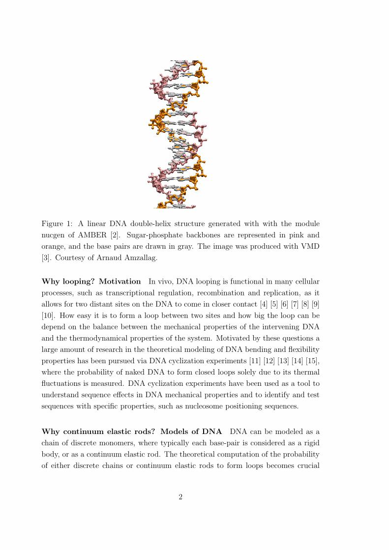
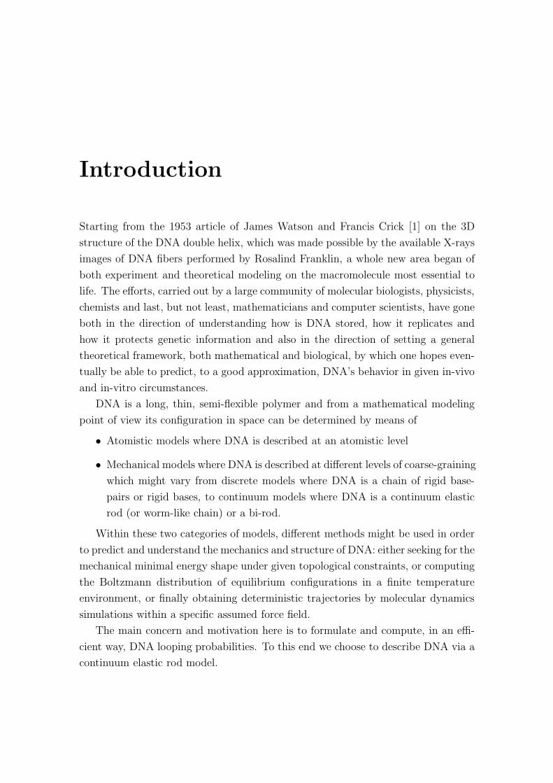
Figure 1: A linear DNA double-helix structure generated with with the module
nucgen of AMBER [2]. Sugar-phosphate backbones are represented in pink and
orange, and the base pairs are drawn in gray. The image was produced with VMD
[3]. Courtesy of Arnaud Amzallag.
Why looping? Motivation In vivo, DNA looping is functional in many cellular
processes, such as transcriptional regulation, recombination and replication, as it
allows for two distant sites on the DNA to come in closer contact [4] [5] [6] [7] [8] [9]
[10]. How easy it is to form a loop between two sites and how big the loop can be
depend on the balance between the mechanical properties of the intervening DNA
and the thermodynamical properties of the system. Motivated by these questions a
large amount of research in the theoretical modeling of DNA bending and flexibility
properties has been pursued via DNA cyclization experiments [11] [12] [13] [14] [15],
where the probability of naked DNA to form closed loops solely due to its thermal
fluctuations is measured. DNA cyclization experiments have been used as a tool to
understand sequence effects in DNA mechanical properties and to identify and test
sequences with specific properties, such as nucleosome positioning sequences.
Why continuum elastic rods? Models of DNA DNA can be modeled as a
chain of discrete monomers, where typically each base-pair is considered as a rigid
body, or as a continuum elastic rod. The theoretical computation of the probability
of either discrete chains or continuum elastic rods to form loops becomes crucial
2
to analyze and understand the available experimental data. A great variety of
literature is available on the topic, including analytical and numerical approaches
in both discrete and continuum models, for instance [13] [16] [17] [18] [19] [20] [21]
[22] [23] [24] [25] [26] [27]. Moreover, to capture a quantitative discrepancy between
theoretical predictions for the cyclization probabilities of short DNA constructs and
recent experimental data [14], several possible physical mechanisms, such as DNA
kinking and bubble formation along the DNA fragment, have been suggested and
analyzed within a generalization of worm like chain models [20] [23]. A less dramatic
breakdown of linear elasticity have also been proposed in [28], where a model, called
the sub-elastic chain, in which the bending energy density is an arbitrary function of
the curvature is considered and have been proven to give rise to greater cyclization
efficiency.
All these mechanisms should enhance the cyclization probability at small scales,
i.e. for short DNA fragments, and yet leave the probability distribution unchanged
at large scales, that is for long DNA fragments. Kinking in small DNA closed loops
has also been detected in molecular dynamic simulations [29]. On the other hand
the experimental data we are referring to is still under debate [15].
Within continuum elastic rod models DNA is pictured as a framed curve de-
scribed by the special Cosserat rod theory [19] [30] [31] [32] [33] [34]. In space, the
rod is an oriented curve defined by a configuration variable q(s) = (r(s),R(s)),
where r(s) (s ∈ [0, L]) is the centerline to the rod and R ∈ SO(3) is the proper
rotation relating a fixed, right-handed, orthonormal frame {ei} in IR3 to the co-
moving orthonormal frame {di(s)}, which changes as the rod is bent and twisted
under the action of an external load. For a linear elastic rod, the associated strain
energy density W (w, s) is quadratic in w, which is defined in terms of the shifted
strains (u− u) and (v− v), where u is the Darboux vector and v is the tangent to
the rod and u, v are their values in the minimum energy shape. Elastic rod models
have proven to be extremely well-suited [19] [32] [33] [34] to the determination of the
mechanical minimal energy configuration. The extension of this approach to include
the correction factor due to the fluctuations around the minimal energy configura-
tion, when a quadratic energy is associated to the system, is the main objective of
this thesis.
Why path integrals? This thesis At room temperature, DNA molecules in
solution are subjected to thermal motion and the polymer is randomly bending and
moving as water molecules and ions collide with it. Once thermal equilibrium is
3
reached with the surrounding medium, the ensemble of admissible configurations to
DNA will most presumably follow a Boltzmann distribution. Looping probability
can thus be expressed as a path integral restricted to a given subset of the admissible
configurations (for instance closed ones) each weighted with its Boltzmann weight
conveniently normalized by the path integral of all admissible configurations.
There are several methods by which computation at the lowest order of ap-
proximation of a path integral can be performed. Usually an expansion of the
action around a minimal energy configuration is considered, as is for instance done
within discrete models of DNA in [13]. However in [13] the equilibrium configura-
tion around which harmonic fluctuations are considered is found with an iterative
algorithm which can be computationally more expensive and manifest convergence
problems when compared to the method based on symmetry breaking and parameter
continuation exploited in [19] for a continuum rod model.
It is worth noting that the crucial assumption used when approximating a path
integral via consideration of only quadratic fluctuations around a minimal energy
configuration is that the energy required to deform the system is large with respect
to KBT . This in turn physically means that we should either consider short enough
fragments of DNA, or the temperature should be low enough. DNA has a char-
acteristic persistence length which is a length scale related to the rate of decay in
space of the correlation between the tangents to the DNA. It has been measured to
be approximately 150 base-pairs or 50 nm, corresponding to 15 helical turns of the
molecule. The approximation of quadratic fluctuations is presumably a reasonable
one if we intend to describe the mechanics of DNA at the length scale of a few per-
sistence lengths or less. This in turn is a length scale of great relevance in biology
as DNA is known frequently to be tightly bent at length scales shorter than the
persistence length [9] [10]. For instance, in a nucleosome particle a total of about
150 base-pairs of DNA is wrapped twice around the protein-complex histones, and
in the Lac-Operon the distance between the two operators may range between 60
and 100 base-pairs [7].
Starting from the assumed Boltzmann distribution for the configurations, our
objective is to incorporate in continuum elastic rod models the computation up to
second-order corrections of the conditioned probability density function for an end
point to be at a fixed point and orientation in space, subject to the other end being
held fixed at the origin of the coordinate framing (which choice involves no loss
of generality assuming invariance of the energy under rigid body motions). This
objective is achieved via analysis of a path-integral formulation of the problem.
4
The final formula for the conditional probability is given by two factors: the first
depends on the energy of a minimal energy configuration satisfying the prescribed
end conditions, while the second accounts for fluctuations around the minimal energy
configuration and is expressed in terms of a determinant of certain Jacobi fields
associated with the second variation of the energy. The formula is robust in that
it remains valid for all of the standard cases arising in DNA modelling, including
sequence-dependence etc. The formula is also highly amenable to a straightforward
numerical evaluation even in rather general cases.
To consider some completely analytically treatable examples we explicitly com-
puted the probability density function for cyclization up to second order corrections,
for the following cases:
• a uniform, not isotropic, extensible and shearable rod.
The stiffness matrix was assumed to be diagonal. The homogeneity assumption
guarantees that the linear differential equations to be solved are constant coef-
ficient ones: in contrast any non uniform model requires numerical treatment.
The formula so obtained has a nice limit for inextensible and unshearable rods,
with no remnant of the shear and extension degrees of freedom.
• a uniform, not isotropic, inextensible and unshearable rod.
Same conditions as in the extensible and shearable case where considered. A
natural transition to a Hamiltonian formulation was exploited as the coefficient
matrices in the Lagrangian formulation diverge as the constrained system is
reached. The formula obtained from the limiting equations is in agreement
with the limit of the previous formula.
5
The thesis is structured as follows.
In Chapter 1 we introduce the special Cosserat theory for rods and we discuss
the basic properties of elastic rods. We introduce the strain energy density for a
most general shearable, extensible elastic rod. We then discuss the optimization
problem in the variational formulation and we re-derive, following [36], the expres-
sions for the first and second variation of the strain energy functional for a shearable
and extensible rod. We also describe the constrained case of an inextensible and
unshearable rod, writing the first and second variation of the constrained energy
functional.
In Chapter 2 we present a path integral method for computing the conditional
probability density of a chain at thermal equilibrium with a heat bath whose en-
ergy density is at most quadratic in its variables. We assume the set of admissible
configurations for the chain to follow a Boltzmann distribution and the existence of
a unique minimal energy configuration. We further assume the temperature scale
to be conveniently small with respect to the mechanical energy stored in the chain.
Using [43], we show that up to quadratic fluctuations about the minimal energy
configuration, the probability density function can be computed by means of the
energy of the minimizer and of a basis of solutions to the Jacobi equations with
appropriate initial conditions.
In Chapter 3 we apply the method derived in Chapter 2 to the specific example
of a shearable and extensible continuum elastic rod. We discuss issues related to the
choice of a measure in the configuration space of oriented curves. We further extend
the method to consider constrained rods, where neither deformations in length nor in
the cross section of the rod are allowed. For this purpose, we exploit the Hamiltonian
version of the second variation of a slightly shearable and extensible rod and show
that, in the limit of negligible shears and extension, the Hamiltonian equations for
the second variation do indeed coincide with Jacobi equations derived in [33] for an
isoperimetrically constrained rod.
In Chapter 4 we consider the example of a uniform, non-isotropic, intrinsically
straight and untwisted linear elastic rod. We compute analytically our approximate
probability density function for the formation of a circular loop. The non-isotropicity
restriction is essential for the application of the method derived in Chapter 2 and 3,
as for this specific boundary conditions, only non-isotropic rod have isolated minima.
All the other assumptions are merely to render the problem solvable by hand.
Conclusions and future directions are discussed in Chapter 5.
6
Chapter 1
Continuum elastic rod models for
DNA
In this chapter we introduce the continuum elastic rod model for DNA, describing
the special Cosserat rod theory [35] by which means a complete treatment of the
rod’s static mechanical behavior is given.
In the special Cosserat rod theory not only deformations such as flexure and
torsion of the the rod are considered, but also deformations along the length of
the rod and in two orthogonal directions on the plane of the rod’s cross section
are allowed. After reviewing the kinematic equations, the balance laws and the
constitutive relations for the rod, we discuss the associated variational formulation.
We give the expressions for the first and second variation of the energy associated
to the rod, which rely on the approach exploited in [36] and will be used in the
following chapters. Finally, we discuss the inextensible and unshearable limit of the
Cosserat rod, which represents the currently preferred model for DNA.
All the material presented in this chapter is known in literature, although the
notation chosen here might differ with others elsewhere. A systematic and compre-
hensive overview on elastic rods can be found in [37], whereas more details on the
variational formulation can be found, in addition to the references already cited in,
for instance [38] [39].
1.1 Special Cosserat model
In space, the rod is an oriented curve defined by a configuration variable q(s) =
(r(s),R(s)), where r(s) (s ∈ [0, L]) is the centerline to the rod (or axis of the rod)
7
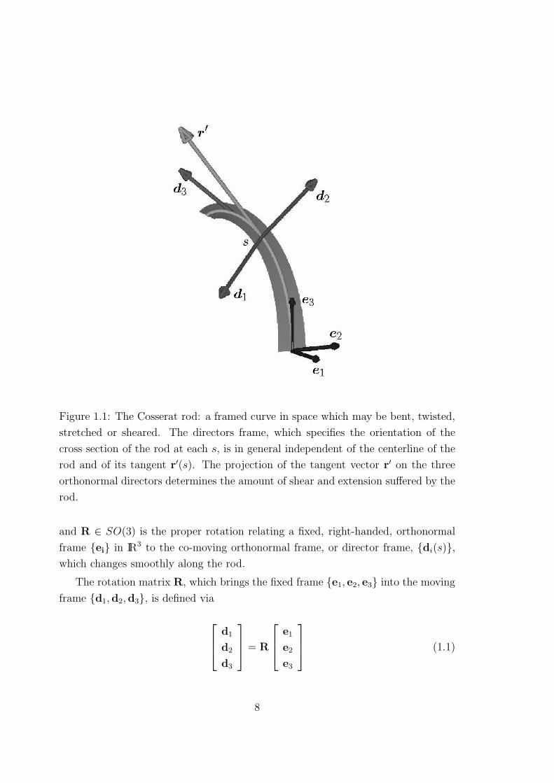
Figure 1.1: The Cosserat rod: a framed curve in space which may be bent, twisted,
stretched or sheared. The directors frame, which specifies the orientation of the
cross section of the rod at each s, is in general independent of the centerline of the
rod and of its tangent r′(s). The projection of the tangent vector r′ on the three
orthonormal directors determines the amount of shear and extension suffered by the
rod.
and R ∈ SO(3) is the proper rotation relating a fixed, right-handed, orthonormal
frame {ei} in IR3 to the co-moving orthonormal frame, or director frame, {di(s)},
which changes smoothly along the rod.
The rotation matrix R, which brings the fixed frame {e1, e2, e3} into the moving
frame {d1,d2,d3}, is defined via
d1
d2
d3
= R
e1
e2
e3
(1.1)
8
or
[d1 d2 d3] = [e1 e2 e3]RT . (1.2)
where [d1 d2 d3] is a matrix whose columns are the vectors d1,d2,d3 expressed in
the fixed frame. Thus, in our notation,
R =
d1 · e1 d1 · e2 d1 · e3
d2 · e1 d2 · e2 d2 · e3
d3 · e1 d3 · e2 d3 · e3
. (1.3)
Note that the role of RT and R can be inverted.
1.1.1 Kinematics
The kinematic equations are the equations defining the strains v(s) and u(s) through
derivatives with respect the parameter s of the directors and of the centerline. The
first equation defines v:
v(s) = r′(s), (1.4)
where r′(s) is the tangent to the centerline and ′ denotes the derivative with respect
to s. The first two components of v(s) with respect to the moving frame, v1(s) =
v(s) ·d1(s) and v2(s) = v(s) ·d2(s), are associated with transverse shearing, whereas
the third component, again with respect to the moving frame, v3(s) = v(s) · d3(s),
is associated with stretching or compression of the rod.
The second equation defines u(s). The orthonormality of the directors di(s)
implies the existence of a strain vector u(s), defined through
d′i(s) = u(s) × di(s), i = 1, 2, 3. (1.5)
The components of the strain vector u(s), often referred to as the Darboux vector,
with respect to the director, co-moving, frame read
ui =1
2ǫijkd
′j(s) · dk(s) (1.6)
if ǫijk is the totally antisymmetric tensor, and summation over equal indices is
understood. In (1.6) the first two components u1(s), u2(s) are the bending strains,
whereas the third component u3(s) is the twist strain. The physical meaning of the
Darboux vector is to indicate the rate at which the co-moving frame is rotating with
respect to the fixed frame. From (1.5) and (1.1) or (1.2) we may also derive
u× = RR′T , (1.7)
9
where u×ik = ǫijkuj reads
0 −u3 u2
u3 0 −u1
−u2 u1 0
, (1.8)
the components ui being with respect to the co-moving frame.
The initial configuration of the rod, typically a configuration in which there is no
external load, is either described through an intrinsic framing {di(s)} or character-
ized by certain intrinsic strains vi(s) and ui(s). Then, v1,2 are the intrinsic shears
whereas v3 is the intrinsic stretch. And u1,2 are the intrinsic curvatures and u3 is
the intrinsic twist. Up to an arbitrary choice of some initial conditions, for instance
the values of the intrinsic framing {di(0)} at s = 0, equations equivalent to (1.4),
(1.5) and (1.6) hold for the intrinsic framing and strains.
1.1.2 Force and balance laws
Assuming that the only external loads are momenta and forces applied at the ends
of the rod, the force and moment balance laws in the fixed frame read
n′ = 0, (1.9)
m′ + r′ × n = 0, (1.10)
where n(s) and m(s) denote respectively the resultant force and the resultant mo-
ment of the material on the side s+ acting on the material on the side s− at each
cross section labeled by s.
1.1.3 Constitutive relations
Constitutive relations are relations connecting the strain vectors u and v the forces
n and the moments m. Under the assumption of hyper-elasticity, there exists a
convex and coercive strain energy density function W (V,U, s) such that
∂W
∂V(0, 0, s) =
∂W
∂U(0, 0, s) = 0 (1.11)
and
ni =∂W
∂Vi
mi =∂W
∂Ui(1.12)
10
where
V = v − v U = u− u (1.13)
and ni, Vi and mi, Ui are respectively the components of the force and strain V and
moment and strain U with respect to the director frame. For linear elastic rods,
which can be extended in length and sheared in the cross section, the strain energy
density depends at most quadratically on the shifted strains V and U, that is
W ≡ W (V(s),U(s)) =1
2[VT (s) UT (s)] P(s)
[
V(s)
U(s)
]
(1.14)
where V and U are defined in (1.13) and P is the stiffness matrix, a positive definite
and symmetric (6 × 6) matrix.
Finally, the energy associated to the continuum linear elastic rod is given by
E[q(s)] =
∫ L
0
W (V,U, s)ds (1.15)
where q(s) is a configuration of the rod (so a certain centerline and a rotation
matrix expressed in some parametrization of SO(3), for example Euler angles or
quaternions as we will see later), L is the length of the rod, while W (V,U, s) is the
strain energy density (1.14).
1.2 The variational formulation
In this section we review the variational formulation of optimization problems for an
elastic rod subject to boundary conditions forcing both ends to be in a prescribed
point of the configuration space. In the context of continuum elastic rods, this in
turn means that position and orientation of the rod are fixed at both ends
q(0) = (r(0),R(0)) = q0 = (r0,R0)
q(L) = (r(L),R(L)) = qL = (rL,RL) . (1.16)
The first order variation of the strain energy (1.15) yields necessary conditions
for equilibrium configurations of (1.15) satisfying (1.16), in the form of the Euler-
Lagrange equations. The second variation of the strain energy (1.15) leads to further
necessary conditions for equilibrium configurations to minimize (1.15). These topics
have been largely addressed in [38] [39] [40] [36].
As is standard, given a configuration q(s) we define [42]
δq(s) (1.17)
11
to be the variation field and, given a parameter α, we define
δE [q(s), δq(s)] =d
dα
∣
∣
∣
∣
α=0
E [q(s) + αδq(s)] ,
δ2E [q(s), δq(s)] =d2
dα2
∣
∣
∣
∣
α=0
E [q(s) + αδq(s)] .
Our aim here is mainly to write an expression for the first and second variation
in order to refer to these expressions later on, rather than discussing extensively
the vast literature on the stability analysis for equilibrium configurations. We are
here concerned with shearable and extensible rods and we will treat the case of
constrained systems separately.
1.2.1 First order variation
In computing the first and second variations to (1.15), we have to introduce the
variation field or perturbation field (1.17). We will use the choice introduced in [36],
where a variation of the rotation matrix R is given through a vector δΘ defined via
the 3 × 3 skew-symmetric matrix
δΘ× = δRTR. (1.18)
Using equation (1.18), there is no need for the moment to worry about choosing a
parametrization of SO(3). The variation field δq(s) = h(s) ∈ R6 then reads
h =
[
δr
δΘ
]
, (1.19)
where the s dependence has been dropped for simplicity of notation but should
always be considered present.
The dependence on the rotation matrix in (1.14) can be read out directly from
(1.4) and (1.7).
Differentiating (1.4) and (1.7) we get
δv = R(δr′ + r′×δΘ), (1.20)
δu = RδΘ′, (1.21)
where δΘ× is defined in equation (1.18).
12
The first variation then reads
δE =
∫ L
0
[(
∂W
∂v
)
· δv +
(
∂W
∂u
)
· δu
]
ds
=
∫ L
0
[
(RTWv) · (δr′ + r′ × δΘ) + (RT Wu) · δΘ
′] ds
=
∫ L
0
[
(−RT Wv)′ · δr + (RTWv) · (r
′ × δΘ) − (RTWu)′ · δΘ
]
ds
= −
∫ L
0
[
(RTWv)′ · δr +
(
(RT Wu)′ + r′ × RT Wv
)
· δΘ]
ds
= −
∫ L
0
[n′ · δr + (m′ + r′ × n) · δΘ] ds, (1.22)
where the linearization of (1.16), which for (1.19) reads
(δr(0), δΘ(0)) = 0,
(δr(L), δΘ(L)) = 0, (1.23)
and the following definitions
n = RT ∂W
∂v(1.24)
m = RT ∂W
∂u(1.25)
are assumed.
At critical configurations
n′ = 0 (1.26)
m′ + r′ × n = 0. (1.27)
Note that as equations (1.26), (1.27) are written they have to be considered in the
fixed frame, as n(s) in (1.24) and m(s) in (1.25) are the resultant force and moment
in the fixed frame. As expected, equations (1.9) and (1.10) are recovered.
Moreover, if we vary RRT instead of RTR, so as to introduce a field
δΨ× = RδRT . (1.28)
from the first variation of the energy, we would get the equations
n′ + u× n = 0 (1.29)
m′ + u× m + v × n = 0 (1.30)
13
where
n = RT n (1.31)
m = RTm, (1.32)
and v, u are given in (1.4), (1.7) and are to be considered as components in the mov-
ing frame. In (1.31) and (1.32), n(s), m(s) are respectively the resultant force and
moment expressed in the moving frame. Equations (1.29), (1.30), are the balance
laws for the rod expressed in the moving frame.
1.2.2 Second order variation
The second variation reads
δ2E =1
2
∫ L
0
[(
∂2W
∂v2δv
)
· δv +
(
∂2W
∂u2δu
)
· δu
]
ds
+1
2
∫ L
0
[
2
(
∂2W
∂u∂vδu
)
· δv +
(
∂W
∂v
)
· δ2v +
(
∂W
∂u
)
· δ2u
]
ds (1.33)
where δv, δu are given in (1.21) and
δ2v = R[
2δr′ + (r′×δΘ)]
× δΘ (1.34)
δ2u = RδΘ′×δΘ. (1.35)
Using expressions in (1.21) and (1.35), the second variation (1.33) becomes
δ2E =1
2
∫ L
0
[(
RT WvvRδr′)
· δr′ +(
RTWuuRδΘ′) · δΘ′ + 2(
RTWuvRδΘ′) · δr′]
ds
+1
2
∫ L
0
[
2δr′ ·(
RT WvvRr′×)
δΘ −(
r′×RTWvvRr′×δΘ)
· δΘ]
ds
+1
2
∫ L
0
[
−2(
r′×RT WuvRδΘ′) · δΘ + RTWu · (δΘ′ × δΘ)
]
ds
+1
2
∫ L
0
[
RTWv · [(r′ × δΘ) × δΘ] + 2RT Wv · (δr
′ × δΘ)]
ds. (1.36)
Rearranging (1.36), one obtains an expression such as (see 2.22)
δ2Estat =1
2
∫ L
0
[
h′TP(s)h′ + hTQ(s)h + 2h′TC(s)h]
ds (1.37)
where h is given as in (1.19) and the 6 × 6 matrices P(s),Q(s),C(s) read
P =
(
RTW vvR RT W uvR
RT W vuR RT W uuR
)
(1.38)
14
Q =
(
0 0
0 −r′×RT W vvRr′× + 12(n×r′× + r′×n×)
)
(1.39)
C =
(
0 RT W vvRr′× − n×
0 RTWvuRr′× − 12m×
)
(1.40)
Note however that as they are written in (1.38), (1.39) and (1.40) the matrices
P(s),Q(s),C(s) are expressed in the fixed frame. Performing a proper orthogonal
rotation on the variable h
h → h = Rh (1.41)
where R is given by
R =
[
R 0
0 R
]
, (1.42)
the second variation becomes
δ2E =1
2
∫ L
0
[
h′TPm(s)h′ + 2h′T[
Pm(s)u×(s) + Cm(s)]
h]
ds
+1
2
∫ L
0
[
hT[
Qm(s) − u×Cm(s) + CTm(s)u× − u×Pm(s)u×] h
]
ds(1.43)
where, u× being defined in equation (1.8),
u× =
[
u× 0
0 u×
]
(1.44)
and Pm(s), Qm(s) and Cm(s) are respectively the matrices P(s),Q(s),C(s) ex-
pressed in the moving frame. In particular this means that for each matrix,
Afixed = RTAmovingR (1.45)
where R is given in (1.42). More specifically the matrices Pm(s), Qm(s) and Cm(s)
read
Pm(s) =
[
Wvv Wuv
Wvu Wuu
]
(1.46)
Qm(s) =
[
0 0
0 −v×Wvvv× + 1
2(n×v× + v×n)
]
(1.47)
Cm(s) =
(
0 Wvvv× − n×
0 Wvuv× − 1
2m×
)
(1.48)
15
where n and m are respectively the resultant force and moment in the moving frame,
as in equations (1.31) and (1.32). Finally, defining
P(s) = Pm(s)
Q(s) =[
Qm(s) − u×Cm(s) + CTm(s)u× − u×Pm(s)u×]
C(s) =[
Pm(s)u× + Cm(s)]
. (1.49)
the second variation (1.43) can be written in a more compact way,
δ2E =1
2
∫ L
0
[
h′T P(s)h′ + 2h′T C(s)h + hT Q(s)h]
ds. (1.50)
1.3 Constrained systems
In the following we consider inextensible and unshearable elastic rods as constrained
systems and we briefly review the constrained variational formulation.
For inextensible and unshearable rods, three degrees of freedom are suppressed
and the following constraints hold
|r′(s)| = 1 ∀s
v1(s) = 0 = v2(s), (1.51)
from which, combined with (1.4), we infer
r′(s) ≡dr
ds= d3(s). (1.52)
The strain energy density (1.14) is now purely a function of the strains u and
the intrinsic strains u so that the energy associated reads
E ≡
∫ L
0
W (U(s), s) ds, (1.53)
where U is defined in (1.13).
The constitutive relations (1.12) only define the moment m, and the force n
becomes a basic unknown to be determined by the equilibrium equations for the
system (1.53).
For inextensible and unshearable rods satisfying the boundary conditions (1.16),
the isoperimetric constraint∫ L
0
r′(s) ds = rL − r0 (1.54)
16
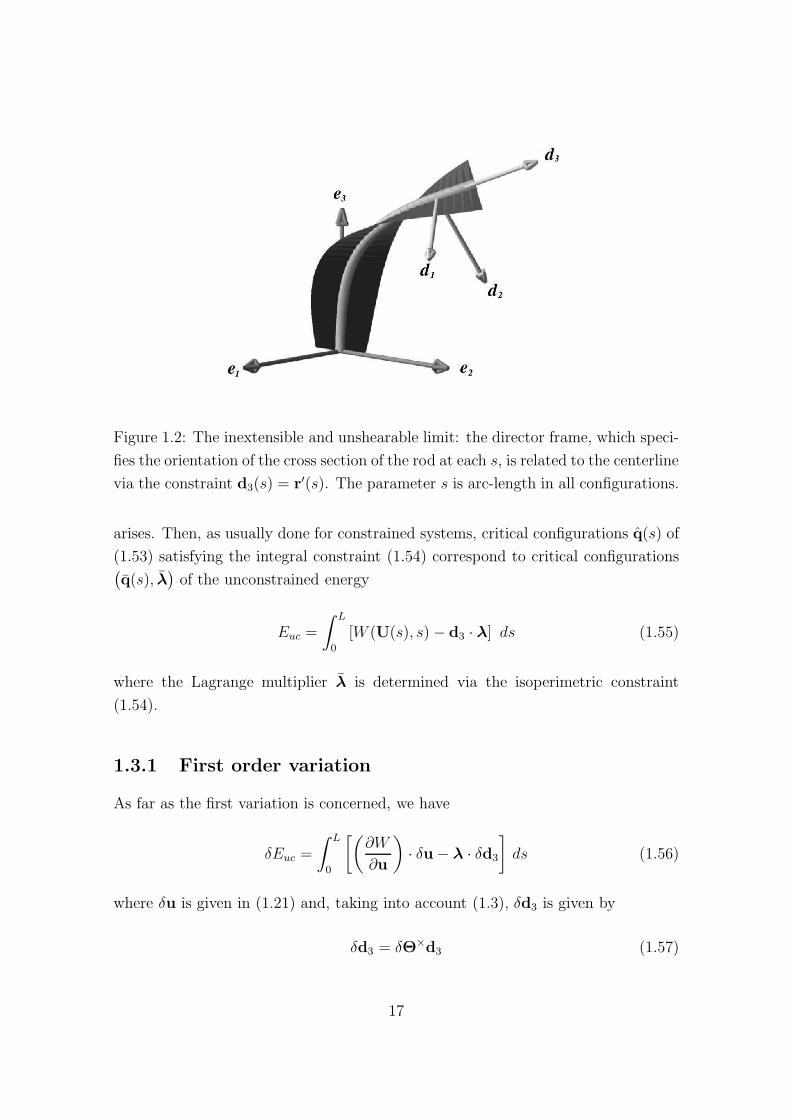
Figure 1.2: The inextensible and unshearable limit: the director frame, which speci-
fies the orientation of the cross section of the rod at each s, is related to the centerline
via the constraint d3(s) = r′(s). The parameter s is arc-length in all configurations.
arises. Then, as usually done for constrained systems, critical configurations q(s) of
(1.53) satisfying the integral constraint (1.54) correspond to critical configurations(
q(s), λ)
of the unconstrained energy
Euc =
∫ L
0
[W (U(s), s) − d3 · λ] ds (1.55)
where the Lagrange multiplier λ is determined via the isoperimetric constraint
(1.54).
1.3.1 First order variation
As far as the first variation is concerned, we have
δEuc =
∫ L
0
[(
∂W
∂u
)
· δu − λ · δd3
]
ds (1.56)
where δu is given in (1.21) and, taking into account (1.3), δd3 is given by
δd3 = δΘ×d3 (1.57)
17
as, in our notation (1.3), the column vector d3 = RTe3. With (1.21) and (1.57),
after performing an integration by parts, the first variation (1.56) becomes
δEuc =
∫ L
0
[((
RT ∂W
∂u
)′− λ × d3
)
· δΘ
]
ds (1.58)
so that the necessary condition for a configuration to be an equilibrium of (1.53)
reads
m′ + d3 × λ = 0 (1.59)
which again is exactly the balance equation (1.10) for the constrained system (1.55)
where λ plays the role of the unknown force n in the fixed frame.
1.3.2 Second order variation
The second variation for the system (1.55) has the same form of (1.37), where the
coefficient matrices are (3× 3) and where the matrix Q has now changed to include
an extra-term associated with the Lagrange multiplier λ. The variation field h has
to satisfy the linearized version of (1.54)
∫ L
0
δd3 ds = 0 (1.60)
so that the ensemble of allowed variation fields Aconst is characterized by
Aconst ≡
{
h ∈ R3 : h(0) = 0, h(L) = 0 and
∫ L
0
δΘ×d3 ds = 0
}
(1.61)
where the integral equation is a vector representation for a system of three scalar
equations, corresponding to the equation (1.60) for each component of δd3. The
second variation thus reads
δ2Euc =1
2
∫ L
0
[(
∂2W
∂u2δu
)
· δu
(
∂W
∂u
)
· δ2u − λ · δ2d3
]
ds (1.62)
where δ2u is defined in (1.35) and δ2d3 is given by
δ2d3 = Θ×Θ×d3. (1.63)
As a function of δΘ the second variation (1.62) has the following form
δ2Euc =1
2
∫ L
0
[
δΘ′T Pc(s) δΘ′ + δΘT Qc(s)δΘ + 2δΘ′T Cc(s)δΘ]
ds (1.64)
18
where
Pc = RT WuuR
Qc = −1
2
(
λ×d×3 + d×
3 λ×) = −
1
2RT(
n×e×3 + e×
3 n×)R
Cc = −1
2m× = −
1
2RTm×R. (1.65)
and the identity(
RT n)×
d×3 = RT n×Rd×
3 = RT n×e×3 R (1.66)
has been used. In (1.65), as in (1.58), the triple λ is intended as the triple of
components of the unknown force in the fixed frame (note that in the moving frame
the components of d3 are of course (0, 0, 1)).
As done for the shearable extensible case, one could then write the second vari-
ation (1.64) in the moving frame. Instead, let us consider the Jacobi system of
equations, which will be of relevance in the rest of the thesis, associated with the
second variation (1.64). The second order system would read
[
Pc (δΘ)′ −1
2m×δΘ
]′−
1
2m× (δΘ)′ −
1
2
(
λ×d×3 + d×
3 λ×) δΘ = 0 (1.67)
or in the Hamiltonian version (first order system)
(δΘ)′ =P−1
c
2m×δΘ + P−1
c δmΘ
(δmΘ)′ =1
2m×P−1
c m×δΘ −1
2
(
λ×d×3 + d×
3 λ×) δΘ
+1
2m×P−1
c δmΘ (1.68)
where
δmΘ = Pc (δΘ)′ −1
2m×δΘ (1.69)
and Pc is given in (1.65). In either case, (1.67) or(1.68), the linearized constraints
(1.60) should also be satisfied.
1.4 Conclusions and summary
In this chapter we have introduced the special Cosserat theory for elastic rods and set
notation for the rest of the thesis. More specifically we have introduced the general
model of an hyper-elastic shearable extensible rod, and re-derived the variational
19
formulation for the first and second variation of the energy functional associated to
the rod following the notation adopted in [36].
The expressions for the first variation can be found in equation (1.22). As far
as the second variation is concerned, the expression in the fixed frame is given in
equation (1.37) and the coefficient matrices in (1.38), (1.39) and (1.40). In the
moving frame the second variation reads as in equation (1.50) where the coefficient
matrices are this time defined in (1.49).
We have then considered an inextensible and unshearable rod, thereafter referred
to as the constrained system, where no stretch nor shear is allowed and the integral
constraint (1.54) must be satisfied. We have then derived the first and second
variation respectively in (1.58) and (1.64), where the coefficient matrices for the
second variation were given in (1.65) and the linearized constraints (1.60) must be
satisfied.
Finally, we have written the Jacobi system of equation for the unshearable and
inextensible case, associated with the second variation(1.64).
20
Chapter 2
General quadratic energy
densities: a path integral approach
for computing conditional
probabilities
In this chapter we focus on computing conditional probabilities for a statistical me-
chanical system at thermodynamical equilibrium. In particular we consider systems
in which the internal potential energy density is at most quadratic in the variables
associated with deviations from an unperturbed or intrinsic state.
We express the conditional probability in terms of a path integral, or functional
integral, and we reproduce the result of [43] for a statistical mechanical system
at equilibrium. In [43] a quantum mechanical system with a general quadratic
Lagrangian is investigated, and the propagator is explicitly computed in terms of
a pre-factor term depending solely on the energy of the classical solution and a
second factor due to quadratic fluctuations around the classical solution, which is
then proven to be equivalent to the inverse square root of the determinant of a
matrix satisfying a second-order non linear differential equation and specific initial
conditions. The proof is carried out via an elegant and concise algebraic argument.
For polymer chains or elastic rods we are interested in real-values path integrals but
the algebraic argument in [43] still applies.
Furthermore we show that the non-linear differential equation derived in [43]
may be transformed into a matrix Riccati equation, which is then known to be
locally equivalent to a second-order linear differential equation [44] [45]: the Jacobi
21
equations, or Euler Lagrange equations for the second order variation of the internal
potential energy. We show that the initial conditions to be satisfied by such Jacobi
fields can be chosen, up to a constant matrix, to be equivalent to those arising in
[43]. We then claim that for our statistical mechanical system the second factor
due to fluctuations around the minimal energy configuration, is given by the inverse
square root of the determinant of a matrix which columns are solutions to the Jacobi
equations for the system at hand.
We believe that the reduction to the Jacobi system is new for the level of general-
ity assumed here. And we remark that it is this level of generality that is necessary
for the application described in Chapter 4 or for any other application aimed at
modeling DNA.
2.1 Statement of the problem
The main objective is to derive the conditional probability density for the ends of a
statistical mechanical continuum chain at thermodynamical equilibrium to be in a
given state, specified by a point in configuration space.
In mathematical terms, our aim translates into computing
ρ[q0,qL; 0 , L ] :=Z (q(s) ∈ Γ)
Z(2.1)
where q(s) ∈ Rm is the configuration variable, s ∈ [0, L] a continuum parameter
defining the position along the length of the chain,
Γ := {q(s) s.t. q(L) = qL} (2.2)
and
Z (q(s) ∈ Γ) =
∫
e−βE[q(s)]D[q(s)]Γ (2.3)
is the conditional partition function, conditional on the end-point of the chain to be
at a fixed point in configuration space, whereas Z is the configurational partition
function
Z =
∫
e−βE[q(s)]D[q(s)]. (2.4)
In both (2.3) and (2.4), β = 1KB T
, KB being the Boltzmann constant and T the
temperature of the system, and E is the internal energy associated to configurations
of the system.
22
We note here that, in order to derive a probability from (2.1), one must integrate
(2.1) over an appropriate volume element in the configuration space of the end of
the chain.
The relation between the conditional (2.3) and the unconditional (2.4) partition
function is given by
Z =
∫
Rm
dqLZ (q(s) ∈ Γ) (2.5)
so that the partition function corresponds to integrating the conditional partition
function in (2.3) over all possible values of the end point of the chain.
Note that in (2.1) we assume the other or initial end of the chain to be held fixed
in configuration space, and we further assume this point to coincide with the origin
in configuration space. This last assumption is of no restriction as in general the
energy E is invariant under rigid body motions. So without loss of generality we
may re-define Γ to be
Γ0 := {q(s) s.t. q(0) = 0 and q(L) = qL} (2.6)
The integrals appearing in (2.3) and (2.4) are path integrals or functional inte-
grals, in that the integration must be carried out on a given (infinite dimensional)
space of functions, which describe the configuration state of the system. Mathemat-
ically path integrals can be viewed as an extension or generalization of the concept
of integral in infinite-dimensional spaces [46] [47] [48] [49].
It is always a delicate matter to define the appropriate path differential, that is
the measure by which the different paths are summed up. In fact one could say that
writing∫
(q0, qL)
e−βE[q(s)]D[q(s)], (2.7)
should corresponds to the action ’summing over all admissible configurations each
weighted with its statistical weight’ but a precise or mathematically rigorous mean-
ing of this action is not yet contained in (2.7).
Different procedures may be followed when performing a path integration as in
(2.7): a typical way is to replace the infinite-dimensional space integral with the
limit for N → ∞ of N copies of finite-dimensional integrals. In this case the path
integral is defined via a limiting procedure, as was done originally by Feynman [46],
and the path integral is in fact truly defined as the appropriate continuous limit of
a finite-dimensional approximation of it.
Otherwise one might, if dealing with Wiener integrals, define the Wiener measure
as a Gaussian-type proper measure on the ensemble of trajectories of the Brownian
23
.
.
.
.
.
.
0
ε
2ε
L
qL
q qq0 1 2
q q1 2
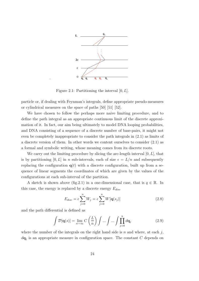
Figure 2.1: Partitioning the interval [0, L].
particle or, if dealing with Feynman’s integrals, define appropriate pseudo-measures
or cylindrical measures on the space of paths [50] [51] [52].
We have chosen to follow the perhaps more naive limiting procedure, and to
define the path integral as an appropriate continuous limit of the discrete approxi-
mation of it. In fact, our aim being ultimately to model DNA looping probabilities,
and DNA consisting of a sequence of a discrete number of base-pairs, it might not
even be completely inappropriate to consider the path integrals in (2.1) as limits of
a discrete version of them. In other words we content ourselves to consider (2.1) as
a formal and symbolic writing, whose meaning comes from its discrete roots.
We carry out the limiting procedure by slicing the arc-length interval [0, L], that
is by partitioning [0, L] in n sub-intervals, each of size ǫ = L/n and subsequently
replacing the configuration q(t) with a discrete configuration, built up from a se-
quence of linear segments the coordinates of which are given by the values of the
configurations at each sub-interval of the partition.
A sketch is shown above (fig.2.1) in a one-dimensional case, that is q ∈ R. In
this case, the energy is replaced by a discrete energy Edisc
Edisc = ǫn∑
j=0
Wj = ǫn∑
j=0
W [q(sj)] (2.8)
and the path differential is defined as∫
D[q(s)] = limn→∞
C
(
L
n
)∫
...
∫
...
∫ n∏
j=0
dqj (2.9)
where the number of the integrals on the right hand side is n and where, at each j,
dqj is an appropriate measure in configuration space. The constant C depends on
24
ǫ = L/n and in fact will be defined in such a way that the limit (2.9) makes sense
(in fact each of the integrals on the right hand side of (2.9) brings in a constant
factor depending on ǫ, for simplicity all these constant factors have been compacted
in C).
2.2 Approximation about the minimal energy con-
figuration
From the point of view of the limiting procedure, the conditional probability density
(2.1) is a ratio of two infinite products of finite-dimensional integrals: the denom-
inator (or normalizing factor) may be explicitly computed if the energy associated
with the system is quadratic in its variables, as then it would correspond to a (in-
finite) product of Gaussian integrals. For the numerator, the boundary conditions
enforcing the second end to be fixed in space complicate the matter, as the domain
of integration of each finite-dimensional integral is no longer Rm, and the Gaussian
integrals cannot be computed directly.
In the literature it is well known that, under specific hypotheses, it is possible
to approximate (2.1) by means of an expansion around the minimal energy config-
uration [43] [47] [48] [49] [52]. This approximation, essentially allows for replacing,
in specific circumstances, a given arbitrary energy with a quadratic energy, as, in
a Taylor expansion of the energy, all orders higher than the second are neglected.
Thus, it gives a first approximation to (2.1) for an arbitrary, and not necessarily
quadratic, energy functional.
In the following we will proceed in computing (2.1), assuming that the main con-
tributions to (2.1) come from the minimizer and the quadratic fluctuations around
it. This assumption is reasonable if β is large compared to the energy functional. In
other words the thermal energy should be small enough compared to the mechan-
ical energy stored in the system, although a precise statement about the range in
which the approximation is valid would require much more care. Practically, this
means that the chain should be stiff enough to resist large deviations due to thermal
motion, so that either the temperature is low enough, or the chain is short enough.
For finite and real integrals, such an approximation relies on the technique of
asymptotic approximation, usually referred as Laplace’s method, to evaluate inte-
grals of the form∫
A
e−N f(t) dt (2.10)
25
where N is a large positive number, f(t) is a continuous and twice differentiable
function which has a minimum at t ∈ A. When performing a Taylor expansion,
the first derivative being zero, one is left with only the second derivative, and the
integral is thus reduced to
e−Nf(t)
∫
A
e−N2
f ′′(t)(t−t)2 dt. (2.11)
The limits of the integral (2.11) are then heuristically extended to infinity, in order to
recover a Gaussian integral, the justification for doing so coming from the argument
that if N is large enough any contribution to the integral from the region other than
[t − δ, t + δ] is arbitrarily small for any fixed small δ.
We will assume that the configuration which minimizes the energy
E[q(s)] =
∫ L
0
W (q(s),q′(s), s)ds q(s) ∈ Rm (2.12)
associated to the system, under the specific boundary conditions in (2.6), is unique.
Of course the set Γ0 (2.6) is not restricted to the unique minimizer: on the contrary
it contains all other configurations which are not minimizers and yet satisfy (2.6).
We will refer to W in (2.12) as the energy density of the system.
If an expansion around the unique minimal energy configuration is performed,
q(s) ≃ q(s) + h(s) (2.13)
where q(s) is the minimal energy configuration and h(s) is the variation field de-
scribing fluctuations about it, we may approximate the energy (2.12) by
E ≃ E|q +1
2hT δ2E|qh (2.14)
as, by definition, on the minimal energy configuration
δE|q = 0. (2.15)
After the expansion (2.14) is performed, the probability density in (2.1) reads
ρ[q0,qL; 0 , L ] ≃e−βE|q
∫
e−β2δ2E|q D[h(s)]
∫
e−βE D[q(s)](2.16)
where now h(s) satisfy the linearized version of the original boundary conditions
(2.6)
h(0) = 0 = h(L). (2.17)
26
Consistent with the finite-dimensional approximation of (2.16), we consider the
following partition of the interval [0, L]
0 = s0 < s1.... < sj .... < sn = L (2.18)
and we define ǫ to be the step of the discretization
ǫ =L
n(2.19)
so that
sj = jǫ j = 0, 1, 2.....n . (2.20)
Finally, the conditional probability density for the chain to have its end-point
fixed in space can be written as
ρ[q0,qL; 0 , L ] ≃e−βE|q
∫
e−β2δ2E|q D[h(s)]
∫
e−βE D[q(s)]
≡ limn→∞
e−βE|q
∫
...∫
...∫
e−β ǫPn
j=0 δ2E[hj ]∏n−1
j=1 dhj∫
...∫
...∫
e−βǫPn
j=0 E[qj]∏n
j=1 dqj
, (2.21)
where we have used the boundary conditions on the configurations contributing to
the conditional probability density function (2.6), so that no integration in either
q0 nor h0 is needed, and moreover no integration on hn is needed (as after the
linearization about the minimal energy configuration, the condition (2.17) must be
satisfied). Here dqj is an appropriate measure in the discretized approximation to
the configuration space of the system, and dhj is an appropriate measure in the
discretized approximation of the tangent space to the configuration space of the
system.
The objective is now to compute explicitly the limit on the right hand side of
(2.21).
2.2.1 Recovering Papadopoulos equations
In this section we re-derive the result originally stated in [43] for a quantum me-
chanical system. For a general quadratic energy density, the second variation reads
δ2E =1
2
∫ L
0
[
h′TP(s)h′ + hTQ(s)h + 2h′TC(s)h]
ds (2.22)
where h satisfies (2.17) and matrices P, Q and C are matrices related to W as
follows
P(s) =∂2W
∂q′∂q′ , Q(s) =∂2W
∂q∂q, C(s) =
∂2W
∂q∂q′ (2.23)
27
Recall that whereas P(s) and Q(s) are symmetric matrices, the matrix C(s) is
neither symmetric nor antisymmetric.
The discretized version of (2.22) then reads
δ2Edisc =1
2ǫ
n−1∑
j=0
[
∆hTj Pj∆hj + ǫ2 hT
j Qjhj + ǫ ∆hTj (Cjhj + Cj+1hj+1)
]
(2.24)
where
∆hj = hj+1 − hj (2.25)
and the mid-point prescription has been used.
Here and afterwards the notation is:
hj = h(sj); Pj = P(sj); Qj = Q(sj); Cj = C(sj) (2.26)
Given the boundary conditions in (2.17),
h0 = h(0) = 0 = h(L) = hn (2.27)
individual terms
−ǫhTj Cjhj + ǫhT
j+1Cj+1hj+1 (2.28)
cancel in the sum, and (2.24) takes the form
1
2ε
n−1∑
j=1
(
hTj
[
Pj + Pj−1 + ε2Qj
]
hj − hTj+1 [Pj − εCj]hj − hT
j [Pj + εCj+1]hj+1
)
(2.29)
Finally, using
hTj+1Cjhj = hT
j CTj hj+1 (2.30)
equality (2.24) becomes
δ2Edisc =1
2ε
n−1∑
j=1
(
hTj
[
Pj + Pj−1 + ε2Qj
]
hj − hTj+1Ljhj − hT
j LTj hj+1
)
(2.31)
where, recalling that Pj is a symmetric matrix,
Lj =[
Pj +ε
2
(
CTj+1 − Cj
)
]
. (2.32)
The best would be to be able to transform (2.31) into a pure quadratic form, i.e. to
write
δ2Edisc =1
2ǫ
n−1∑
j=1
ΘTj AjΘj (2.33)
28
for some vector Θ in Rm and some (m × m) symmetric matrix A. Note however
that the quadratic form cannot be as simple as
(hj − hj+1)TAj(hj − hj+1) (2.34)
for then comparing with (2.31) we would get
Aj = Lj (2.35)
from the mixed terms, whereas
Aj =(
Pj + Pj−1 + ǫ2Qj
)
(2.36)
from the quadratic terms.
Papadopoulos cleverly proposes [43]
Θj = hj − Bjhj+1 (2.37)
where
BTj Aj = Lj
AjBj = LTj (2.38)
and
A1 = P0 + P1 + ǫ2Q1
Aj+1 = Pj + Pj+1 + ǫ2Qj+1 − BTj AjBj. (2.39)
Note that the definition (2.39) takes into account that at each successive step (j +1)
the unwanted term
hTj+1B
Tj AjBjhj+1
cancels.
Hopefully now that we have reduced (2.31) to (2.33) through definitions (2.38)
and (2.39), we can compute the limit on the right hand side of (2.21), which reads
limn→∞
ρ(n−1)[0, L] (2.40)
where, taking into account (2.33),
ρ(n−1)[0, L] ≡
√
detβ
2πǫP0
∫
Rm(n−1)
n−1∏
k=1
√
det
(
β
2πǫPk
)
e− β
2ǫ
n−1P
j=1ΘT
j AjΘjn−1∏
k=1
dΘk
(2.41)
29
where the integral is m(n − 1)-fold, so that (2.41) is in fact a product of (n − 1)
integrals each of which has to be computed in Rm and the factors involving the
determinant of the matrices Pk are due to the integration of the normalizing factor,
as we will explicitly show in Chapter 3 for elastic rods (3.61).
We remark that the change of variables (2.37) has the important feature that the
Jacobian of the transformation is one. In fact, as Θj only depends on hj and hj+1,
the Jacobian matrix is an m(n− 1)× m(n− 1) upper triangular matrix. Moreover,
the (m×m) block matrices on the diagonal all have ones on their diagonal, so that
the determinant of the Jacobian matrix for the transformation (2.37) is exactly one.
We will see later that the only useful changes of variables in path integrals are those
for which the Jacobian matrix of the discrete change of variables is a triangular
matrix.
Evaluating the Gaussian integrals as in equation (3.60), equation (2.41) becomes
ρ(n−1) =
√
detβ
2πǫP0
(
β
2πǫ
)m(n−1)/2 (2πǫ
β
)m(n−1)/2[
det
n−1∏
k=1
PkA−1k
]1/2
= ǫ−m/2
√
detβ
2πP0
[
detn−1∏
k=1
AkP−1k
]−1/2
=
√
detβ
2πP0
[
det ǫ
n−1∏
k=1
AkP−1k
]−1/2
=
√
√
√
√
√detβ
2π
(
ǫP−10
n−1∏
k=1
AkP−1k
)−1
(2.42)
where we have used the properties of determinants and in particular that the deter-
minant of a product of matrices is invariant under permutations of the matrices.
So, what is the message of (2.42)? The message is that ρ(n−1) can be computed
as the inverse square root of the determinant of some matrix which in fact is the
product of (n − 1), (m × m) matrices. One can therefore visualize ρ(n−1) as the
inverse square root of the determinant of huge block diagonal matrix,
A1 (P1)−1 . . . 0
.... . .
...
0 · · · A(n−1)P−1(n−1)
(2.43)
where each block is itself a (m×m) matrix (so that the total dimension of the matrix
is (m(n − 1) × m(n − 1)). As n goes to infinity, the matrix (2.43) becomes infinite,
30
so the idea is to use the fact that in (2.42) there is a factor ǫ in front of the infinite
productn−1∏
k=1
AkP−1k (2.44)
which somehow will help, and then to compute ρ as the limit of ρ(n−1) when n goes
to infinity through (2.40).
Defining the (m × m) matrix Dn to be
Dn ≡ ǫ P(0)−1n∏
k=1
AkP−1k , (2.45)
it is clear that
Dn+1 = DnAn+1P−1n+1 (2.46)
and this is the recurrence relation we are seeking. From (2.46), one immediately
gets
An+1 = D−1n Dn+1Pn+1
A−1n = P−1
n D−1n Dn−1. (2.47)
Furthermore equations (2.39), (2.38) and (2.32) yield
An+1 = Pn + Pn+1 + ǫ2Qn+1 − BTnAnBn
= Pn + Pn+1 − PnA−1n Pn + ǫ2Qn+1
− ǫ
[
CTn+1 − Cn
2
]
A−1n Pn − ǫPnA
−1n
[
Cn+1 − CTn
2
]
− ǫ2
[
CTn+1 −Cn
2
]
A−1n
[
Cn+1 −CTn
2
]
. (2.48)
Using the recurrence relation (2.47) and multiplying on the left by Dn, transforms
expression (2.48) into
Dn+1Pn+1 = DnPn + DnPn+1 − Dn−1Pn + ǫ2DnQn+1
− ǫDn
[
CTn+1 − Cn
2
]
P−1n D−1
n Dn−1Pn − ǫDn−1
[
Cn+1 − CTn
2
]
− ǫ2Dn
[
CTn+1 −Cn
2
]
P−1n D−1
n Dn−1
[
Cn+1 − CTn
2
]
(2.49)
For convenience, we rewrite (2.49) in the following way
A − B = −C − D (2.50)
31
where
A =(Dn+1 −Dn)
ǫ2Pn+1 −
(Dn − Dn−1)
ǫ2Pn (2.51)
B = DnQn+1 (2.52)
C = Dn
[
CTn+1 −Cn
2ǫ
]
P−1n D−1
n Dn−1Pn + Dn−1
[
Cn+1 −CTn
2ǫ
]
(2.53)
D = Dn
[
CTn+1 −Cn
2
]
P−1n D−1
n Dn−1
[
Cn+1 − CTn
2
]
. (2.54)
Adding and subtracting the term
(Dn − Dn−1)Pn+1
to (2.51) implies
A =
[
Dn+1 − 2Dn + Dn−1
ǫ2
]
Pn+1 +
[
Dn − Dn−1
ǫ
] [
Pn+1 − Pn
ǫ
]
. (2.55)
Defining
Csn =
Cn + CTn
2(2.56)
it follows that
Dn−1
[
Cn+1 − CTn
2ǫ
]
= Dn−1
[
Csn+1 − Cs
n
ǫ
]
+ Dn−1
[
CTn+1 −Cn
2ǫ
]
. (2.57)
Moreover taking into account
P−1n D−1
n DnPn = ]1
and adding and subtracting
Dn
[
CTn+1 − Cn
2ǫ
]
,
expression (2.53) becomes
C = Dn
[
Cn − CTn+1
2
]
P−1n D−1
n
[
Dn − Dn−1
ǫ
]
Pn
+ Dn−1
[
Csn+1 −Cs
n
ǫ
]
−
[
Dn −Dn−1
ǫ
] [
Cn − CTn+1
2
]
. (2.58)
32
Finally then equation (2.50) can be written as
[
Dn+1 − 2Dn + Dn−1
ǫ2
]
Pn+1 +
[
Dn − Dn−1
ǫ
] [
Pn+1 − Pn
ǫ
]
− DnQn+1 + Dn−1
[
Csn+1 −Cs
n
ǫ
]
=
[
Dn − Dn−1
ǫ
] [
Cn −CTn+1
2
]
− Dn
[
Cn −CTn+1
2
]
P−1n D−1
n
[
Dn −Dn−1
ǫ
]
Pn
+ Dn
[
Cn −CTn+1
2
]
P−1n D−1
n Dn−1
[
Cn+1 − CTn
2
]
. (2.59)
Taking the limit as n → ∞ or equivalently ǫ → 0, as (2.19) is valid, equation (2.59)
becomes the Papadopoulos equation [43]
d
ds
(
dD
dsP
)
+ DdCs
ds− D
[
Q + CaP−1Ca]
=
dD
dsCa − DCaP−1D−1dD
dsP, (2.60)
where
Cs =C + CT
2
Ca =C − CT
2. (2.61)
The initial conditions for the (matrix) solution D(s) of the second order differ-
ential equation (2.60) are the following
D(0) = 0[
dD(s)
ds
]∣
∣
∣
∣
0
= P(0)−1 (2.62)
because
limǫ→0
D1 = 0 (2.63)
limǫ→0
[
D1 −D0
ǫ
]
= P(0)−1. (2.64)
33
From definition (2.45)
D1 = ǫP−10 A1P
−11 (2.65)
and as ǫ → 0, given (2.32), (2.38) and (2.39), we have
A1 → [P0 + P1] (2.66)
so that
limǫ→0
D1 = limǫ→0
ǫP−10 [P0P
−11 + ]1 ] = lim
ǫ→02 ǫP−1
0 = 0, (2.67)
because
limǫ→0
P0P−11 = ]1 . (2.68)
For (2.64) a similar argument holds. Again from equation (2.45)
D2 − D1 = ǫP−10 A1P
−11 [A2P
−12 − ]1 ] (2.69)
and this time, as ǫ → 0,
A2 → [P1 + P2] − P1A−11 P1 (2.70)
so that
[A2P−12 − ]1 ] → [ ]1 − P1A
−11 ]P1P
−12 . (2.71)
Finally taking into account that (see (2.67))
limǫ→0
P1P−12 = ]1
limǫ→0
A1P−11 = 2 ]1 (2.72)
we obtain
limǫ→0
[
D1 − D0
ǫ
]
= limǫ→0
ǫP−10 A1P
−11
ǫ[A2P
−12 − ]1 ]
= 2P−10
1
2]1 = P−1
0 , (2.73)
and this completes the proof.
Following the approach of [43], the expression for (2.21) is thus given by
ρ[q0,qL; 0, L] ≃ e−βE|q∫
e−β2δ2E|q D[h(s)]
= e−βE|q
√
det
(
β
2πD−1(L)
)
(2.74)
where D(s) satisfies (2.60) with the initial conditions (2.62).
34
2.3 A formula for the second order correction
In this section we show that even in the presence of real cross terms, the Papadopou-
los matrix is intimately related to the Jacobi matrix, or matrix of Jacobi solutions,
so that the final formula for the second order correction to the probability density
function (2.1) can be expressed in terms of the inverse square root of Jacobi matrix
evaluated at the final end of the arc-length interval.
2.3.1 Relating Papadopoulos to Jacobi
We recall here, for sake of simplicity, the Papadopoulos equation
[
D′P + DCT]′− D′C − DQ
=
DCaP−1Ca − [DCa]′ −DCaP−1D−1D′P. (2.75)
Furthermore we recall that the Jacobi equations for the second variation (2.22) read
[Ph′ + Ch]′− CTh′ − Qh = 0 (2.76)
or
[Ph′]′= − (Cs)′ h− [Cah]′ − Cah′ + Qh, (2.77)
where the matrices P, Q and C are defined in (2.23) and h ∈ Rm. Here and in the
following: ′ = dds
.
We claim that the non-linear change of variables, for s 6= 0,
V−1V′ = D−1D′ + CaP−1 (2.78)
relates (2.75) to (2.76) in the sense that D satisfies (2.75) if and only if each column
of a matrix H = VT , where V is defined via (2.78), satisfies (2.76). Moreover if the
initial conditions for D are
D(0) = 0, D′(0) = P−1(0) (2.79)
then the initial conditions for V can be chosen, up to a left factor consisting in a
constant invertible matrix, the same
V(0) = 0, V′(0) = P−1(0). (2.80)
35
Before we continue, we make two quick remarks: first, the change of variable
(2.78) is well defined as long as V(s) and D(s) are invertible, which in particular,
given (2.79), immediately implies s 6= 0 and the requirement that s should not be a
conjugate point, where the matrix V(s) would become singular.
Second, due to the symmetry of the matrix P, the initial conditions (2.80) imply
the following initial conditions for the m independent solutions hj=1...m of the Jacobi
equations (2.76), constituting the columns of the matrix H,
hj(0) = 0
h′j(0) = P−1
j (0) (2.81)
where P−1j (0) is the jth column of matrix P−1(0).
We first prove our claim directly and then discuss the origin of transformation
(2.78). Assume D to be a matrix satisfying (2.75) and V to be a matrix defined
through (2.78), then differentiating both sides of (2.78), gives
−[
V−1V′]2 P + V−1V′′P +[
V−1V′]P′
=
−[
D−1D′]2 P + D−1D′′P +[
D−1D′]P′ + (Ca)′ , (2.82)
where we made use of the equality
dA−1
ds= −A−1dA
dsA−1 (2.83)
valid for a non singular square matrix A. Recalling (2.78) and the hypothesis that
D satisfies (2.75), gives on the right hand side of equation (2.82)
−[
V−1V′]2 P + 2[
V−1V′]Ca − (Cs)′ + Q + (Ca)′ (2.84)
so that, comparing the left and the right hand sides of (2.82), we derive the following
equation for V
[V′P]′= −V (Cs)′ + [VCa]′ + V′Ca + VQ, (2.85)
which exactly states that each column (or row) of a matrix H = VT must satisfy
(2.77).
Conversely, suppose now V satisfies (2.85) and define a matrix D via equation
(2.78). Then, analogously differentiating both sides of (2.78), on the left hand side
of (2.82) we obtain
−[
D−1D′]2 P−CaP−1D1D′P− (Cs)′ +(Ca)′ +D−1D′Ca +Q+CaP−1Ca. (2.86)
36
Finally, equating (2.86) with the right hand side of (2.78), forces D to satisfy (2.75).
Thus, we conclude that the non-linear transformation (2.78) allows for a map-
ping between solutions to the Papadopoulos equation (2.75) and solutions to the
Jacobi equation for the second variation of the energy functional for which the Pa-
padopoulos equation was derived.
As far as the initial conditions are concerned, the behavior for small values of s
of V−1V′ has to be the same of D−1D′ + CaP−1 which in turn, given the singular
initial conditions on D, is dominated by the behavior of D(s) in the proximity of
s = 0. Specifically, taking into account the initial conditions on D(s) given in (2.79),
we can consider the Taylor expansion of D(s) around s = 0,
D(s) ≃ P(0)−1 s +1
2D′′(0) s2 +
1
6D′′′(0) s3 + O(s3). (2.87)
Assuming the matrices V(s),Ca(s) and P(s) also to have a Taylor expansion in
s = 0, that is:
V(s) ≃ V(0) + V′(0) s +1
2V′′(0) s2 +
1
6V′′′(0) s3 + O(s3)
Ca(s) ≃ Ca(0) + (Ca)′ (0) s +1
2(Ca)′′ (0) s2 +
1
6(Ca)′′′ (0) s3 + O(s3)
P(s) ≃ P(0) + P′(0) s +1
2P′′(0) s2 +
1
6P′′′(0) s3 + O(s3), (2.88)
we should then equate, on each side of (2.78), the coefficient matrices of the different
powers of s. In particular on the right hand side of (2.78), we have
1
s: ]1
s0 :P(0)D′′(0)
2+ Ca(0)P−1(0)
s1 :P(0)D′′′(0)
3−
(P(0)D′′(0))2
4+ (Ca)′ (0)P−1(0) −Ca(0)P−1(0)P′(0)P−1(0)
· · · : · · · (2.89)
where we have used the fact that for all s P(s) is a positive definite matrix, and
therefore invertible. On the left hand side, assuming (2.88) with V(0) not singular,
there would be no term balancing 1/s, as
s0 : V−1(0)V′(0)
s1 : V−1(0)V′′(0) −(
V−1(0)V′(0))2
· · · : · · · (2.90)
37
Furthermore, if V(0) 6= 0 is a singular matrix, then multiplying (2.78) on the left
by V(s), then, as s → 0, on the left hand side we would have
s0 : V′(0)
s1 : V′′(0)
· · · : · · · (2.91)
whereas, on the right hand side we would have
1
s: V(0)
s0 : V′(0) + V(0)
[
P(0)D′′(0)
2+ Ca(0)P−1(0)
]
s1 :V′′(0)
2+ V′(0)
[
P(0)D′′(0)
2+ Ca(0)P−1(0)
]
+ V(0)
[
P(0)D′′′(0)
3−
(P(0)D′′(0))2
4+ (Ca)′ (0)P−1(0) − Ca(0)P−1(0)P′(0)P−1(0)
]
· · · : · · · (2.92)
so that again there would be no correct compensation of the different powers of s.
We therefore conclude that necessarily V(0) = 0. Finally, from the requirement
that the matrix V(s) constructed via (2.78) should be an invertible matrix except
for s = 0, we further conclude that necessarily V′(0) is a non singular matrix.
Of course the foreseen argument does not imply that there are no solutions to the
Jacobi equation (2.76) with an initial condition V(0) 6= 0. Instead, our conclusion is
that if the Jacobi solution is generated by a solution to the Papadopoulos equation
with initial conditions (2.79) through (2.78), then it must similarly start off from
V(0) = 0 and an invertible V′(0). The opposite implication is also true.
Assuming now V(0) = 0 and V′(0) invertible, on the left hand side we have:
1
s: ]1
s0 :[V′(0)]−1
V′′(0)
2
s1 :[V′(0)]−1
V′′′(0)
3−
(
[V′(0)]−1V′′(0)
)2
4· · · : · · · (2.93)
so that as long as (2.90) and (2.93) correctly counterbalance there is an arbitrariness
in the choice of V′(0). We shall then choose the initial value problem (2.80) for V.
38
We note here that both equations (2.75) and (2.76) are invariant under a trans-
formation of variables which multiplies on the left by a constant and invertible
matrix M, so that D and V are solutions to (2.75) and (2.76) related by (2.78),
then also MD and MV are solutions of the corresponding Papadopoulos and Jacobi
equations with initial conditions
D(0) = V(0) = 0, D′(0) = V′(0) = MP−1(0) (2.94)
2.3.2 Riccati matrix equations
We now discuss the origin of transformation (2.78). The key argument is that
equation (2.75) is in fact a matrix Riccati equation, which are known [44] [45] [53]
to be locally equivalent to second-order linear ordinary equations. This last result
is known since the late twenties and relies on the work of Radon [44] [53].
In the following we consider the case in which the coefficient matrices in (2.75)
are constant matrices: a similar argument can be carried out for the more general
case of equation (2.75) with non constant coefficient matrices. By a symmetric
Riccati matrix equation we mean the following equation [44] [53]
Y′ + YKY = G −BTY −YB (2.95)
where all the matrices appearing are assumed to be (n × n) and in principle could
depend on some independent variable s, and the matrices K and G are assumed to
be symmetric.
The Papadopoulos equation (2.75) with constant coefficient matrices reads
D′′P− D[
Q + CaP−1Ca]
= D′Ca − DCaP−1D−1D′P (2.96)
with initial conditions
D(0) = 0, D′(0) = P−1(0). (2.97)
We now show that equation (2.96) falls in the class of equations of the form
(2.95). Recalling that P is symmetric and positive definite, we may define Z to be
Z = DP1/2 (2.98)
in which case equation (2.96) becomes, after multiplying on the right by P−1/2,
Z′′ − Z[
Q +(
Ca)2]
= Z′Ca − ZCaZ−1Z′ (2.99)
39
where
Q = P−1/2QP−1/2
Ca = P−1/2CaP−1/2. (2.100)
and we are assuming s 6= 0. Finally, multiplying equation (2.99) on the right by Z−1
and defining
W = Z−1Z′ (2.101)
we obtain
W′ + W2 = J +[
W, Ca]
(2.102)
where J =[
Q +(
Ca)2]
is a symmetric matrix and
[
W, Ca]
= WCa − CaW. (2.103)
Equation (2.102) is then of the form (2.95) with K = ]1 , G = J and B = −Ca.
Following [45], if we write W as a function of a new non singular matrix variable X
W = FTX−1dX
dsF (2.104)
where F is an orthogonal matrix uniquely determined by the Cauchy problem
dF
ds= FCa F(0) = ]1 , (2.105)
then, given that W satisfies (2.102),
X′′ = XFJFT . (2.106)
Further defining
V = XF (2.107)
implies that V satisfies
V′′ − 2V′Ca − VQ = 0. (2.108)
Defining
V = P−1/2VP−1/2 (2.109)
we get the transposed Jacobi equation (2.76) for constant coefficient matrices
V′′P− 2V′Ca − VQ = 0. (2.110)
Finally, using (2.98), (2.101), (2.104) and (2.105), which in turn imply
W = V−1V′ − Ca, (2.111)
we obtain the non-linear change of variables between D and V
V−1V′ = D−1D′ + CaP−1. (2.112)
40
2.3.3 The final formula
In the previous subsections we have obtained a non-linear transformation of variables
(2.78) which relates a matrix solution of (2.75) to a matrix which columns are
solutions of (2.76): we shall now derive a relation for the determinants of the two
matrices. Taking the trace of both sides of (2.78), we obtain
tr
[
V−1dV
ds
]
= tr
[
D−1dD
ds
]
(2.113)
because, from the elementary properties of the trace, the symmetry of P, and the
asymmetry of Ca
tr[
CaP−1]
= tr[
P−1Ca]
= tr[
(
P−1Ca)T]
= −tr[
CaP−1]
(2.114)
⇓
tr[
CaP−1]
= 0. (2.115)
Moreover for a non-singular matrix,
tr[
A−1A′] =1
detA(detA)′ (2.116)
where equality (2.116) is easy to prove and well known. It suffices to write the
matrix A in Jordan form
A = PDJP−1, (2.117)
where DJ is an upper triangular matrix with the eigenvalues of A on the diagonal,
then
tr[
A−1A′] = tr[
(
DJ)−1 (
DJ)′]
=
∑
i
∏
k
(
dδik
dsλk
)
∏
l λl
=1
detA(detA)′. (2.118)
From (2.113) and (2.116), we have
1
detV(detV)′ =
1
detD(detD)′
⇓
detV(s) = c detD(s) (2.119)
41
where c is some constant. To prove now c ≡ 1, we consider
lims→0
det(
V(s)D−1(s))
. (2.120)
From the Taylor expansions (2.87) and (2.88) that we have considered before, we
obtain
V(s)D−1(s) ≃ V(s)1
s
[
P(0) −P(0)D′′(0)P(0)
2s + O(s)
]
≃
[
P−1(0) +V′′(0)
2s + O(s)
][
P(0) −P(0)D′′(0)P(0)
2s + O(s)
]
=
[
]1 + V′′(0)P(0) s−D′′(0)P(0)
2s + O(s)
]
(2.121)
which in turn implies that the limit (2.120) is 1. Finally if the limit (2.120) is 1,
then in an appropriate neighborhood of s = 0, c = 1, which proves c ≡ 1.
Finally, from (2.119) we can conclude that, although V(s) and D(s) are different
matrices satisfying different equations, their determinant is the same.
Thus, from (2.74), we can further conclude that the conditional probability den-
sity function for a chain to have its end at a fixed point q(L) = qL in space is given,
up to quadratic corrections, by
ρ[q0,qL; 0, L] ≃ e−βE|q∫
e−β2δ2E|q D[h(s)]
= e−βE|q
√
det
(
β
2πV−1(L)
)
(2.122)
where each column of VT (s) satisfies the linear equations (2.76) or Jacobi equations
and the initial conditions (2.81). Formula (2.122) is our main result.
2.4 Conclusions and discussion
In this chapter we have derived an expression for the conditional probability density
of a statistical mechanical chain to have its end point fixed in space, given that the
other end is held fixed at the origin of the configuration space.
The derivation relies on the assumption that, at equilibrium, the collection of
the configurations available to the system follows a Boltzmann distribution and on
the assumption that, at sufficiently low temperatures, there exists a unique minimal
energy configuration around which quadratic fluctuations are considered. We use an
42
algebraic argument first used in [43] to show that the contribution due to quadratic
fluctuations accounts for the square root of the inverse Jacobi matrix built with
solutions to the Jacobi equations with specific initial conditions.
We show that the Papadopoulos equations appearing in [43], whose non-linearity
arises from the presence of a cross term in the second order variation of the energy
functional, are connected via some Riccati equations to the Jacobi linear equations
of the system. This result is quite obvious if there are no cross terms present or if the
coefficient matrix of the cross term is symmetric, as in this case the Papadopoulos
equations simply collapse to the Jacobi equations. But other than these and other
special cases the non-linearity is unavoidable [55], making the connection to the
Jacobi field, satisfying the linear Jacobi equations, at least unclear.
For Feynman path integrals the connection between the Van-Hove-Morette de-
terminant and the Jacobi matrix is well-known: the Van-Hove-Morette determinant,
appearing in the semi-classical approximation to Feynman’s progator (correspond-
ing to the transition amplitude of a position-position transition) is the negative
inverse of a (2n × 2n) Jacobi matrix [48] [52] [54]. In [48] a direct proof, by using
the Gelfand-Yaglom method [56], is given for a one-dimensional system whose La-
grangian does not contain cross terms. In the handbook of Feynman path integrals
[57] one does indeed find the semi-classical approximation to the Feynman kernel
for a general quadratic Lagrangian with cross terms expressed as a function of the
Jacobi solutions, but no reference is made to the Papadopoulos equations and the
Papadopoulos matrix.
Moreover, we note here that although the analytical continuation to negative
imaginary time or space, may be useful to compare and point out analogies between
the real valued path integrals, or Wiener integrals, and complex valued path inte-
grals, or Feynman integrals, complex cross terms are not mapped to real cross terms.
In facti
~
∫
[
x′T Ax′ − xT Bx + x′TCx]
dt
⇓
for t → t = −iβ~
⇓
−β
∫
[
xT Ax + xT Bx − i xT Cx]
dt (2.123)
where ˙ := ddt
and M = M(t) for each coefficient matrix, so that a direct application
of the formula provided in [57] to the problem of computing (2.1) for a general
43

quadratic energy function is not straightforward.
To the best of our knowledge, our result, without being a surprise, provides a
new proof of the connection between the second order quadratic approximation to
conditional path integrals and the Jacobi fields.
44
Chapter 3
Conditional probability densities
of elastic rods
In this chapter we focus on the problem of computing conditional probability densi-
ties for an elastic rod subject to thermal fluctuations. We assume that, at thermal
equilibrium with the heat bath, the ensemble of admissible configurations of the rod
follows a Boltzmann probability distribution. We also assume the elastic rod to have
a unique minimal energy configuration between the prescribed boundary conditions
on the location and frame orientation at both end points.
The main result of the previous chapter is that, even in the presence of real cross
terms in the second variation, the second order correction to the probability density
function is given by the inverse square root of the determinant of a matrix of solutions
to the Jacobi equations for the functional energy associated to the system. Indeed
continuum elastic rods do in general exhibit a cross term in the second variation of
the strain energy.
For elastic rods the configuration space is the space of framed curves, as was seen
in Chapter 1. We discuss issues related to the choice of an appropriate invariant
measure in this configuration space, and we compute the conditional probability
density for an elastic rod to have its end fixed both in position and orientation, up
to quadratic corrections.
45
3.1 Configuration space and setting of the prob-
lem
In this section we first define the configuration space for continuum elastic rods and
we then set the context for the subsequent computations.
For elastic rods, the functional space over which the functional integrals in (2.1)
are integrated, is the space of framed curves, so that the variable q(s) is here a
couple (r(s),R(s)) where, ∀s, r(s) ∈ R3 and R(s) ∈ SO(3). We recall that the
smooth vector r(s) gives the position of a material point on the rod as a function
of s, whereas R(s) indicates the orientation in space of the cross section at s of the
rod. We can therefore think of q(s) as a couple of independent trajectories: one in
R3 and the second in SO(3).
Different parametrizations are possible for SO(3). In order to avoid difficulty that
can arise from the non simple connectivity of SO(3), it is often convenient to con-
sider, instead of SO(3) itself, its universal covering SU(2). Furthermore any matrix
in SU(2) can be parametrized by a quadruple of real numbers γ = (γ4, γ1, γ2, γ3)T
such that
γ · γ = γ24 + γ2
1 + γ22 + γ2
3 = 1. (3.1)
The quadruple γ = (γ4, γ1, γ2, γ3)T satisfying (3.1) is also called a set of Euler
parameters or quaternions.
If we regard the Euler parameters as Cartesian coordinates in a 4-dimensional
Euclidean space, the group parameter space is thus the surface of the unit sphere in
R4. However, if γ is a unit quaternion corresponding to a given rotation then −γ,
its opposite, corresponds to the same rotation, so that the correspondence from unit
quaternions (or SU(2)) to SO(3) is 2 to 1. This occurrence can be seen directly
if, recalling that by Euler’s theorem each element of the group manifold SO(3) is
equivalent to a rotation of an angle Φ about a unit vector y, the Euler parameter
are expressed as a function of Φ and y as follows
γ4 = cos
(
Φ
2
)
, γk = yk sin
(
Φ
2
)
∀ k = 1, 2, 3. (3.2)
From (3.2) it is in fact clear that if γ corresponds to the pair (y, Φ) then −γ
corresponds to the pair (y, Φ + 2π).
Restricting ourselves to consider one hemisphere of the unit sphere in R4 so as
to remove the double covering, we can introduce for the quaternions the following
46
global parametrization, adapted to the minimal energy configuration
γ(s) =
√
√
√
√1 −3∑
m=1
cm(s)2 γ(s) +3∑
m=1
cm(s)Bmγ(s) (3.3)
where γ(s) is the one-parameter family of quaternions associated with a minimal
energy configuration q(s) for the energy associated with the elastic rod and the
matrices Bm are defined as follows
B1 =
0 0 0 1
0 0 1 0
0 −1 0 0
−1 0 0 0
, B2 =
0 0 −1 0
0 0 0 1
1 0 0 0
0 −1 0 0
,
B3 =
0 1 0 0
−1 0 0 0
0 0 0 1
0 0 −1 0
, (3.4)
and satisfy the algebra
BiBk = −δik ]1 − ǫiklBl, (3.5)
where ǫikl is the total antisymmetric or Levi-Civita tensor and summation over equal
indices is intended.
After parametrization (3.3) and from now on, we consider the configuration
variable describing the elastic rod to be
q(s) = (r(s), c(s)) (3.6)
where r(s) ∈ R3 and c(s) lives in the unit ball in R
3.
We now follow the approach outlined in Chapter 2. The energy E associated to
a linear elastic rod is
E[q(s)] =
∫ L
0
W (V,U, s)ds, (3.7)
where the strain energy density function reads (cf. Chapter 1)
W (V(s),U(s)) =1
2[VT (s) UT (s)] P(s)
[
V(s)
U(s)
]
, (3.8)
V and U are defined in (1.13), and P is the stiffness matrix. The energy density
in (3.8) is quadratic in the shifted strains. We assume that there exists a unique
minimizer
q = (r(s), c(s)) (3.9)
47
for (3.7) with both position and orientation fixed at both ends.
We consider fluctuations around the unique minimal energy configuration (3.9)
as follows
r(s) ≃ r(s) + δr
c(s) ≃ c(s) + δc, (3.10)
and, consistently, we define the variation field h(s) to be
h(s) = (δr(s), δc(s)) . (3.11)
Performing an expansion of (3.7) around the minimal energy configuration, we
write
ρ[(0, 0) , (r(L), c(L)) ; 0 , L ] ≃e−βE
∫
e−β2δ2E D[h(s)]
∫
e−βE D[q(s)](3.12)
where E and δ2E are the strain energy and the second variation of the strain energy
(3.7) evaluated at the minimizer (3.9) and q(s) and h(s) are respectively defined in
(3.6) and (3.11).
In (3.12), the functional integral in the denominator is over all framed curves
satisfying the Dirichlet boundary condition at one end
q(0) = q0 = (0, 0) , (3.13)
whereas the functional integral in the numerator is over all framed curves satisfying
the Dirichlet boundary conditions at both ends
h(0) = h0 = (0, 0) = h(L) = hn = (0, 0) . (3.14)
It is worth noting that the boundary conditions (3.13) correspond physically to
setting
r(0) = 0, and R(0) = ]1 , (3.15)
which in turn implies that the director frame coincides with the fixed frame at s = 0.
In fact, since both by γ(s) and γ(s) must satisfy (3.13), requiring (3.15) implies
γ(0) = γ0 = γ(0) = γ0 =
0
0
0
1
(3.16)
48
which in turn, given (3.3), implies
c(0) = c0 = 0 ⇒ (cm)0 = 0 ∀m. (3.17)
According to Chapter 2, we interpret the approximate expression for the proba-
bility density function in (3.12) as the limit, for large n, of
e−βE
∫
...∫
...∫
e−β ǫPn
j=0 δ2E[hj ]∏n−1
j=1 dhj∫
...∫
...∫
e−βǫPn
j=0 E[qj]∏n
j=1 dqj
, (3.18)
where we assume a partition of the interval [0, L] as in (2.18) has been previously
accomplished. The step of the discretization and the finite values sj are respectively
given by (2.19) and (2.20).
We first define the appropriate measure dqj and then proceed to the computation
of the limit (3.18).
3.2 Measure
The measure on the whole space of framed curves can be chosen, up to a multiplica-
tive constant, to be the product of an invariant measure on E(3) and of an invariant
measure on S0(3) [58] [59]. A natural invariant measure on E(3) is the Lebesgue
measure. On S0(3), a Haar bi-invariant measure, that is right and left invariant,
may be uniquely defined up to a constant factor [59].
In both [59] and [60] a procedure is presented in order to define an invariant
measure on S0(3) for any given parametrization of the group. In particular for
unit quaternions, or Euler parameters, which provide a four dimensional global and
two-to-one parametrization of S0(3), the infinitesimal volume measure dqj at each
j would read [60]
dqj = drj δ
(
1 −∑
k
γ2k, j
)
dγj (3.19)
where γk, j = γk(sj), so that the volume measure on S0(3) becomes a surface
(Lebesgue) measure on the unit sphere in R4.
Taking into account the discretized version of (3.3)
γj =
√
√
√
√1 −3∑
m=1
(cm, j)2γj +
3∑
m=1
cm, jBmγj (3.20)
49
we may now consider rk, j = rk(sj) (k = 1, 2, 3) and cm, j = cm(sj) (m = 1, 2, 3) to
be the variables on which integration is carried out, so that, the volume measure
dqj at each j becomes
dqj =d r1, j d r2, j d r3, j d c1, j d c2, j d c3, j
√
1 −∑3
m=1 (cm, j)2
(3.21)
where for each j = 1...n the vector cj lives in the unit ball in R3:
3∑
m=1
(cm, j)2 < 1. (3.22)
The expression (3.21) can be obtained recalling that for any regular surface M
embedded in an Euclidean space parametrized by
ψ : B ∈ Rn → R
m (3.23)
where B is an open set, so that for any point p ∈ M : p = ψ(b1, b2, ...bn), a metric
tensor is naturally induced on the tangent space TpM at any point p ∈ M on the
surface, by
gik = ψi ·ψk (3.24)
where
ψi ≡∂ψ
∂bi(3.25)
are the coordinate vectors in TpM , which provide a basis for TpM , and (·) is the
scalar product defined in the ambient space. By means of (3.24), the area element
on the surface is given by
dA =√
det(gik) d b1 ∧ d b2 ∧ d b3... ∧ d bn (3.26)
where ∧ is the wedge product.
In this specific case, the parametrization (3.3) γ (c) defines the coordinate vectors
in the tangent space to be
∂γ
∂ci
= Biγ −ci
√
1 −∑3
m=1 (cm)2γ (3.27)
which in turn, given the orthonormality of the basis {B1γ, B2γ, B3γ, γ} of R4,
implies the metric (3.24) to be
gik =ci ck
(
1 −∑3
m=1 c2m
) + δik, for i, k = 1, 2, 3. (3.28)
50
Finally, from (3.28) we obtain
√
det(gik) =1
√
1 −∑3
m=1 c2m
(3.29)
so that on each j-slice, the expression (3.21) is recovered.
Lastly, for reasons that will become clearer in the next paragraph, we prefer to
perform the following change of variable
y(s) =c(s)
√
1 −∑3
m=1 (cm, (s))2(3.30)
after which the parametrization (3.3) becomes
γ(s) =1
√
1 +∑3
m=1 ym(s)2
[
γ(s) +
3∑
m=1
ym(s)Bmγ(s)
]
(3.31)
or
γj =1
√
1 +∑3
m=1 (ym, j)2
[
γj +3∑
m=1
ym, jBmγj
]
. (3.32)
Our final expression for the measure (3.21) thus reads
dqj =d r1, j d r2, j d r3, j d y1, j d y2, j d y3, j
[
1 +∑3
m=1 (ym, j)2]2
. (3.33)
Note that as the change of variable (3.30) is introduced, the domain of integration
for each of the variables y1, y2, y3, given (3.22), is effectively all of R.
From now on, we will assume the measure to be (3.33).
3.3 Unconstrained systems
Having define the appropriate measure on the configuration space of framed curves,
our objective is now the computation of the approximate probability density function
as defined in (3.18) where the measure dqj is given in (3.21) and where, assuming
(3.10), the linearized measure dhj is defined as
dµhj =d δr1, j d δr2, j d δr3, j d δc1, j d δc2, j d δc3, j
√
1 −∑3
m=1 (δcm, j)2
. (3.34)
We will now compute the limit (3.18), first computing the normalizing factor.
51
3.3.1 Normalizing factor
In order to compute the limit (3.18), we first integrate explicitly the normalizing
product of integrals
∫
...
∫
...
∫
e−βǫPn
j=0 W [qj ]n∏
j=1
dqj . (3.35)
Change of coordinates
Taking into account the form of the strain energy density (3.8), the discretized
version of (3.7) reads
Edisc =ǫ
2
n−1∑
j=0
[VTj UT
j ] Pj
[
Vj
Uj
]
(3.36)
where we have defined, as in Chapter 2,
Vj = v(sj) − v(sj), Uj = u(sj) − u(sj), Pj = P(sj), (3.37)
and have adopted the convention that the shifted strains at the index j are those
locating qj+1 with respect to qj, recalling that the strains and intrinsic strains are
associated with the relative position of two subsequent slices of the framed curve.
Recalling that the intrinsic strains v(s), u(s) are assigned functions of s, describing
the intrinsic state (curvature, twist, stretch and shear) of the rod, we regard v(sj)
and u(sj) as prescribed at each j.
Thus, in order to complete the integration of the integrals in (3.35), we need
to insert the Jacobian of the transformation from the discretized strains {(vj ,uj)}j
to the discretized variables {(rj, cj)}j where the index j now runs from j = 0 to
j = (n − 1). Note that whereas the variable cj was constrained to live in a 3-
dimensional ball of unit radius, at each j the strains, as the vector yj , may take any
real value. This in turn is relevant for the feasibility of evaluation of the integrals
in (3.35), which will be shown to be Gaussian integrals.
From Chapter 1 we have learned that the strain v depends on both the centerline
and the rotation matrix R(s), whereas the strain u depends solely on the rotation
matrix. The (6n × 6n) Jacobian matrix J will then be an upper triangular block
matrix, where each block is a (3n × 3n) matrix
J =
(
J1(vj , rj) J∗(vj,yj)
0 J2(uj ,yj)
)
. (3.38)
52
The aim being the computation of the determinant of J, we will only need to compute
the (3n×3n) Jacobian matrix J1 of the discretized strains {vj}j with respect to the
discretized variables {rj}j and the (3n × 3n) Jacobian matrix J2 of the discretized
strains {uj}j with respect to the discretized variables {yj}j. We stress that as the
change of coordinates involved are global ones, a priori we will have to verify whether
the determinant of J (and therefore the determinants of J1,2) can be factorized in
the product of n determinants, one for each measure j. This indeed will be the case.
Computation of J1
From (1.4), we have
vj = Rjrj+1 − rj
ǫ(3.39)
so that, for each j, vj only depends on rj+1 and rj (as follows directly from the
definition of v in terms of the tangent vector r′). Therefore, J1 is itself an upper
triangular block matrix, and the computation of the determinant only involves the
computation of the determinants of the diagonal block matrices. In fact the matrix
J1 reads
J1 =
∂v0i
∂r0k
∂v0i
∂r1k
0 0 0 ... ... 0
0∂v1
i
∂r1k
∂v1i
∂r2k
0 0 ... ... 0
......
0 ... ... ...∂v
ji
∂rjk
∂vji
∂rj+1k
... 0
0 ... ... ... ...∂v
j+1i
∂rj+1k
... 0
......
0 ... ... ... ... ...∂v
n−2i
∂rn−2k
∂vn−2i
∂rn−1k
0 ... ... ... ... ... ...∂v
n−1i
∂rn−1k
. (3.40)
The diagonal blocks of J1 are the (3 × 3) matrices
∂vi, j
∂rk, j
= −1
ǫRik (3.41)
so that the determinant of J1 simply becomes
(n−1)∏
j=0
∣
∣
∣
∣
∂vi, j
∂rk, j
∣
∣
∣
∣
=
(n−1)∏
j=0
1
ǫ3. (3.42)
Computation of J2
The dependence of the strain u on the quaternions γ can be read from the following
identity [40] (and references therein)
ui = u · di = 2γ ′ · Biγ (3.43)
53
where {di} is the director frame (cf. Chapter 1) and the skew symmetric matrices
Bi are defined in (3.4). Note that the scalar product is again the scalar product of
the ambient space R4 which is inherited by the tangent space at each point of the
smooth manifold. Discretizing (3.43), yields
ui, j =2
ǫ[(γj+1 − γj) · Biγj]
=2
ǫ[γj+1 · Biγj] (3.44)
where in the last equivalence we have used the properties of the matrices Bi (3.5).
From (3.44) and (3.32) it is evident that J2, as J1, is once again an upper triangular
block matrix, so that its determinant is simply the product of the determinants of
the diagonal block (3 × 3) matrices. The diagonal block matrices of J2 read
∂ui, j
∂yk, j= −
2
ǫ αj
[
Bi γj+1 ·
(
Bkγj −yk, j γj
αj
)]
. (3.45)
where we have defined
αj =
√
√
√
√1 +3∑
m=1
(ym, j)2. (3.46)
We note that
∣
∣
∣
∣
∂ui, j
∂ck, j
∣
∣
∣
∣
=23
ǫ3
∣
∣
∣
∣
∣
∣
∣
∣
∣
(B1γj+1)T
(B2γj+1)T
(B3γj+1)T
(γj)T
((
B1γj −y1, jγj
αj
) (
B2γj −y2, jγj
αj
) (
B3γj −y3, jγj
αj
)
γj
)
∣
∣
∣
∣
∣
∣
∣
∣
∣
(3.47)
as, recalling (3.20) and the orthonormality of the basis {B1γ, B2γ, B3γ, γ} of R4,
for each fixed k
γj ·
(
Bkγj −yk, j γj
αj
)
= −yk, j
αj
+1
αj
(
3∑
m=1
ym, jBmγj · Bkγj
)
= 0, (3.48)
where αj was defined in (3.46).
As far as the computation of the determinant of the right matrix in (3.47) is con-
cerned, we first notice that the linear parts in γj do not contribute to the determi-
nant. In fact, recursively developing the determinant by the first column containing
54
a multiple of γj we obtain:∣
∣
∣
∣
(
B1γj −y1, jγj
αj
) (
B2γj −y2, jγj
αj
) (
B3γj −y3, jγj
αj
)
γj
∣
∣
∣
∣
= |B1γj B2γj B3γj γj| .
(3.49)
Then, developing the determinant remaining in (3.49) by the last column and using
(3.32) as well as the orthormality of the basis {B1γ, B2γ, B3γ, γ} of R4, gives
1
αj+
∣
∣
∣
∣
∣
B1γj B2γj B3γj1
αj
3∑
m=1
ym, jBmγj
∣
∣
∣
∣
∣
=1
αj. (3.50)
For the left matrix in (3.47), it is convenient to write
γj+1 = ηj γj +ǫ
2
3∑
k=1
uk, jBkγj (3.51)
where ηj is fixed by the normalization
ηj =
√
√
√
√1 −ǫ2
4
3∑
k=1
(uk, j)2. (3.52)
Referring to (3.51) and (3.52), the determinant of the left matrix in (3.47) reads
(ηj)3 +
ǫ2
4ηj
3∑
k=1
(uk, j)2 (3.53)
which then, again by definition (3.52), is equivalent to ηj .
In conclusion, the determinant of J2 reads
(n−1)∏
j=0
∣
∣
∣
∣
∂ui, j
∂yk, j
∣
∣
∣
∣
=
(n−1)∏
j=0
23
ǫ3
ηj
α4j
. (3.54)
Gaussian integrals
Finally, we are able to compute the discretized version of the functional integral
corresponding the normalizing factor, as in (3.35)
∫
...
∫
...
∫
e−βPn−1
j=0 W (Vj ,Uj)n−1∏
j=0
[
ǫ6
23ηj
]
dVj dUj (3.55)
where now
dVj dUj = dvj duj = d v1, j d v2, j d v3, j d u1, j d u2, j d u3, j , (3.56)
55
and the discretized energy is defined in (3.36). We notice that for each j the αj
appearing in (3.54) cancels with the αj appearing in (3.33). As far as the factor η−1j
is concerned, we use the hypothesis on ǫ to be small, in order to write
η−1j ≃ 1 +
ǫ2
8
[
VTj UT
j
]
E
[
Vj
Uj
]
(3.57)
where
E =
(
0 0
0 ]1
)
. (3.58)
Recalling that, in n dimensions and if M is a real and symmetric (n × n) matrix,
the integral∫
Rn
e−xT Mxxl xm dx (3.59)
is finite and that the Gaussian integral reads
GD(M) =
∫
Rn
e−xT Mx dx = πn/2(
detM−1)1/2
, (3.60)
(3.35) is computed to yield
(n−1)∏
j=0
1
23
√
det
(
2πǫ
βP−1
j
)
(
1 + 0(
ǫ2))
. (3.61)
3.3.2 Probability density function
Taking into account the result in (3.61), we are left with the computation of the
following limit
limǫ→0
∫
...
∫
...
∫ (n−1)∏
j=0
23
√
det
(
β Pj
2πǫ
)
e−β ǫPn
j=0 δ2E[hj ]n−1∏
j=1
dhj , (3.62)
where dhj is given in (3.34). We remark here an important point: under the hypoth-
esis made that the energy functional depends at most quadratically on its variables,
the matrices Pj do not depend on the specific minimal energy around which an ex-
pansion of the functional energy is considered. In fact, for elastic rods, recalling both
expressions (1.38) and (1.46), it appears clear that the matrix P contains informa-
tion only on the specificity of the material under consideration (i.e. the stiffnesses)
and not on the specificity of the configuration assumed by the system. Similarly for
any given energy functional which is at most quadratic in its variables the matrix P
56
defined in (2.23) will not depend on the configuration variable q nor on q′, although
it might still depend on the independent variable s. It is this occurance that allows
for a simplification between the matrices Pj coming from the integration of the par-
tition function and the matrices Pj arising from the integration of the conditional
partition function, which is computed by means of an approximation around the
minimal energy configuration. In fact for the case of general quadratic functional
energies, although the coefficient matrices of the second variation of the functional
energy are to be considered evaluated at the minimal energy configuration, the coef-
ficient matrix P will be equivalent, at each s, to the coefficient matrix P evaluated at
any other configuration. If the assumption of a general quadratic functional energy
is removed, the simplification is no longer possible, and different Pj will arise from
the integration of the numerator and denominator in equation (2.21).
Recalling the expressions derived for the second variation of the energy functional
(3.7) in Chapter 1, given in (1.37) if with respect to the fixed frame or in (1.50) if
expressed with respect to the moving frame, and the definition of the variation field
(1.19), we realize that, in order to evaluate (3.62), we need first to compute a final
change of coordinates.
Change of coordinates
In the following paragraph we compute the Jacobian associated with the change of
coordinates from the linearized variables δΘ to the linearized variables δy. This
computation is necessary as we have chosen to express the second variation in terms
of the variables δΘ, as exploited in [36]. We regard the rotation matrix R as a
function of the quaternion γ, and taking into account (3.3), we can write
R(γ) = R(γ) +∂R
∂γ
∣
∣
∣
∣
γ
δγ (3.63)
where we define R(γ) ≡ R to be the rotation matrix associated with the minimal
energy configuration and from (3.31)
δγ =3∑
s=1
δysBsγ (3.64)
. Recalling our notation (1.3) and (1.18), we thus have
δΘ× = δRT R = δRT R. (3.65)
57
In the following, as before, summation over repeated indices is intended. Therefore
δΘ1 = RT2kδRk3 = 2
[
δy1(d2 × d3)1 + δy2(d3 × d1)1 + δy3(d1 × d2)1
]
δΘ2 = RT3kδRk1 = 2
[
δy1(d2 × d3)2 + δy2(d3 × d1)2 + δy3(d1 × d2)2
]
δΘ3 = RT1kδRk2 = 2
[
δy1(d2 × d3)3 + δy2(d3 × d1)3 + δy3(d1 × d2)3
]
(3.66)
where we have used the definition of the rotation matrix (1.3)
Rik = di · ek (3.67)
and [40] (and references therein)
(
∂d1
∂γ
)T
= 2 [B3γ ⊗ d2 −B2γ ⊗ d3]
(
∂d2
∂γ
)T
= 2 [B1γ ⊗ d3 −B3γ ⊗ d1]
(
∂d3
∂γ
)T
= 2 [B2γ ⊗ d1 −B1γ ⊗ d2] (3.68)
so that, recalling (3.64), for each fixed k, j,
δRkj =∂Rkj
∂γ
∣
∣
∣
∣
γ
· δγ
=∂(dk · ej)
∂γ
∣
∣
∣
∣
γ
· δγ
= 2[
ǫkmlBlγ(
dm · ej
)]
· δγ
= 2ǫkml
(
dm · ej
)
δyl. (3.69)
From (3.66) it is easy to see that the (3(n−1)×3(n−1)) matrix J of the coordinate
transformation Θi, j → y, j is a block diagonal matrix where each block on the
diagonal is the (3 × 3) matrix
Jjd = 2
[
dj1 d
j2 d
j3
]
(3.70)
which has as columns the components of the intrinsic director frame {dk}k with
respect to the fixed basis. The Jacobian therefore reads
n−1∏
j=1
23 = 23(n−1). (3.71)
58
Final expression
We are now able to provide the final expression for the probability density function
conditional on one end of the elastic rod being fixed in location and orientation, and
up to quadratic fluctuations around the minimal energy configuration. Taking into
account (3.61) and (3.71), we can write
ρ[(0, 0) , (r(L), c(L)) ; 0 , L ] ≃ e−βE
∫
...∫
...∫
e−β ǫPn
j=0 δ2E[hj ]∏n−1
j=1 dhj∫
...∫
...∫
e−βǫPn
j=0 E[qj ]∏n
j=1 dqj
=
limǫ→0
2 e−βE
√
det
(
β (P0)
2πǫ
)∫
R6 (n−1)
(n−1)∏
j=1
√
det
(
β Pj
2πǫ
)
e−β ǫPn
j=0 δ2E[hj ]
n−1∏
j=1
dhj
(3.72)
where hj and the measure dhj are now given by
hj = (δrj, δΘj)
dhj =d δr1, j d δr2, j d δr3, j d δΘ1, j d δΘ2, j d δΘ3, j
[
1 + 14
∑3m=1 (δΘm, j)
2]2(3.73)
where (3.66) and the orthonormality of the directors frame have been used. We are
now in the position to apply the algebraic machinery described in Chapter 2, and
correspondingly to compute the limit (3.72) as in section (2.2.1), where now the
coefficients of the discretized second variation of the energy (3.7) are the discretized
version of the matrices (1.38), (1.39) and (1.40) if the second variation is expressed
in the fixed frame (1.37) or are given by the discretized version of the matrices (1.49)
if the second variation is expressed in the moving frame (1.50). We note however
that a novelty here is represented by the correction term, or weight factor at each j
given by1
[
1 + 14
(
δΘTj δΘj
)]2 (3.74)
which, in our approximation would account for a modified, with respect to the
procedure followed in section (2.2.1), differential path
n−1∏
j=1
dhj
(
1 −1
2hT
j Ehj + 0(
hTj hj
)2)
(3.75)
where E is defined in (3.58). The exact physical meaning of correction term (3.74)
is not entirely clear, although, evidently it arises from the topology of SO(3), nor
59
is it clear under which conditions it can be neglected. Its presence could change
the derivation of the Papadopoulos equations, and perhaps lead to a different set of
Jacobi equations. Observing that (3.74) is always smaller than one (as ΘTj δΘj > 0),
and for the purpose of this thesis, we have set the approximation of the probability
density to correspond to the upper limit of (3.72). Accordingly to Chapter 2, we
can thus compute the upper limit approximation of the probability density function
for an elastic rod to have one end fixed in location and orientation as
ρ[(0, 0) , (r(L), c(L)) ; 0 , L ] ≃ 2 e−βE|q
√
det
(
β
2πV−1(L)
)
(3.76)
where the matrix VT satisfies the standard Jacobi system associated with the second
variation (1.37) or (1.50) depending on whether the fixed frame or the moving frame
are chosen (this choice is completely free as no additional Jacobian is involved, given
that the moving frame is merely a rotation of the fixed one). Note that in (3.76)
the additional factor 2 is a vestige of the choice (3.19) for the measure: in fact
quaternions correspond to half angles, as is clear from (3.2). In order to get the
correct (approximate) probability function, it is necessary to integrate over a volume
with the same measure expressed in quaternions.
3.4 Constrained systems
In the previous paragraphs we have applied the result (2.122) derived for a gen-
eral statistical mechanical chain subject to thermal fluctuations, to a shearable and
extensible elastic rod. Although DNA is certainly shearable and extensible, the
stiffnesses associated with deformations in the cross section and in extension are
higher than those associated with bending and twisting, for which reason models
of DNA are normally considered to be inextensible and unshearable discrete chains
and continuum rods. We thus wish to consider a slightly extensible and shearable
rod and to investigate the limit of the probability density function (2.122) as the
shear and extension degrees of freedom become negligible.
To this end, we first start with a remark. If we were to scale the shears by a
factor ω > 0, then the stiffness matrix in the moving frame would read
P =
(
A/ω2 B/ω
BT /ω K
)
(3.77)
60
where B is an arbitrary matrix. As the limit ω → 0 is considered some of the entries
of the stiffness matrix will diverge, whereas the inverse stiffness matrix
P−1 =
(
ω2A−1[
]1 + B(
K − BTA−1B)−1
BTA−1]
−ωA−1B(
K −BTA−1B)−1
−ω(
K − BTA−1B)−1
BTA−1(
K − BTA−1B)−1
)
(3.78)
will stay finite, as
limω→0
P−1 =
(
0 0
0(
K − BTA−1B)−1
)
. (3.79)
Note that the stiffness matrix P in (3.77) is positive definite if and only if the
matrices A and its Schur complement(
K− BTA−1B)
are so, and in this case, the
inverse matrix (3.78) is well-defined.
The main result of our derivation is the reduction of the computation of the ap-
proximate conditional probability density function to the computation of the Jacobi
field associated with the second variation of the energy. We are thus interested in
looking at what happens to such Jacobi fields in the limit ω → 0. In particular we
notice that once the scaling (3.77) is introduced, some of the entries of the coeffi-
cient matrices of the second variation either expressed as in (1.37) or (1.50) for a
shearable extensible rod, will explode as ω is sent to zero, and that the Lagrangian
form of the Jacobi system of equation is not well-defined.
Instead, according to (3.77), the Hamiltonian form of the system of Jacobi equa-
tion is well-behaved.
For sake of simplicity we now consider the example of a diagonal stiffness matrix
(3.77) so that in particular B = 0. The Jacobi equations associated to the second
variation (1.37) read
−[Ph′ + Ch]′ + CTh′ + Qh = 0 (3.80)
where the matrices P, Q and C are given in (1.38), (1.39) and (1.40). As follows
from the derivation of the approximate probability density function, we need 6
independent solutions to (4.14) and we require the following initial value conditions
for the independent Jacobi fields ∀j = 1...6
hj(0) = 0 (3.81)
h′j(0) = P−1
j (0). (3.82)
However with P of the form (3.77), the equation (3.80) has no limit as ω → 0.
61
In contrast, the Hamiltonian form of (3.80) reads
z′ = JSz (3.83)
where
J =
[
0 ]1
− ]1 0
]
, S =
[
−(
Q −CTP−1C)
−CTP−1
−P−1C P−1
]
(3.84)
and
z =
[
h
µ
]
(3.85)
where
µ = Ph′ + Ch (3.86)
is the conjugate variable to the perturbation field h of the configuration variable
q. Moreover, given the initial conditions on the variation field h (3.82) we have the
following initial condition for zj, ∀j = 1...6
zj(0) =
[
hj(0)
µj(0)
]
=
[
0
ej
]
. (3.87)
The matrices in (3.84) are of the form seen in (1.38), (1.39) and (1.40) but now
with the assumption that the stiffness matrix is (3.77) in the moving frame and
B = 0. Thus, they read
P =
(
RT AωR 0
0 RTKR
)
(3.88)
Q =
(
0 0
0 −r′×RT AωRr′× + 1
2(n×r′× + r′×n×)
)
(3.89)
C =
(
0 RT AωRr′× − n×
0 −12m×
)
(3.90)
From (3.88), (3.89) and (3.90), we can now verify that the product of the matrices
J and S defined in (3.84) has a finite limit as ω → 0
limω→0
JS
=
62
0 −r′× 0 0
0 12RTK−1Rm× 0 RTK−1R
0 0 0 0
0 −12(r′×n× + n×r′) + 1
4m×RTK−1Rm× −r′× 1
2m×RTK−1R
(3.91)
Correspondingly the system of Jacobi equations reads
(δr)′ = δΘ×r′
(δΘ)′ =1
2RTK−1Rm×δΘ + RTK−1RδmΘ
(δmr)′ = 0
(δmΘ)′ =1
4m×RTK−1Rm×δΘ
−1
2
(
n×r′×
+ r′×n×)
δΘ
+1
2m×RTK−1RδmΘ − r′
×δmr (3.92)
The system of equations (3.92) is completely equivalent to the system (1.68)
taken with the linearized integral constraint (1.60). The equivalence is evident if we
recall that, in the inextensible unshearable case, the Lagrange multiplier λ plays the
role of the unknown force (and the triplet λ corresponds to the components of the
force in the fixed frame, here n); r′ = d3, and that RTK−1R corresponds to P−1c
defined in (1.65).
Moreover, the first equation in (3.92) is stating
δd3 = δΘ × d3 (3.93)
which we have already computed in (1.57), whereas the third equation is fixing the
linearization of the forces to be constant in the fixed frame. Thus, given the initial
conditions (3.87), of the six independent solutions of (3.92), three will correspond
to vanishing linearized forces, and the three constant linearized forces e1, e2 and e3.
In other words for three solutions
(δmr) (s) = 0, (3.94)
and for the other three
(δmr)i (s) = ei i = 1, ...3. (3.95)
The system of equation (3.92) in fact coincides with the system of equations
introduced in [40] [33] to define an isoperimetric conjugate point method for testing
the stability of the critical configurations of a constrained rod. Therein a (6 ×
63
6) constrained stability matrix M(s) is defined, whose determinant vanishes at
isoperimetric conjugate points and whose construction requires the solutions of three
homogeneous first order Jacobi equations, and three non-homogeneous first Jacobi
equations. The initial value problem considered there to determine the matrix M(s)
corresponds to (3.92) with (3.87), taking into account (3.94) and (3.95). With
respect to the notation of [33], for the three non-homogeneous solutions
Ti = r′×
(δmr)i = d3×ei. (3.96)
We thus conclude that the limiting Jacobi system in (3.92) does indeed corre-
spond to the constrained Jacobi system one could derive from (1.55) as in (1.68).
Furthermore the initial value problem (3.87) is exactly the initial value problem to
consider when constructing the constrained stability matrix M(s) for isoperimetri-
cally constrained systems.
3.5 Conclusions and discussion
In this chapter we have applied the results of Chapter 2 to linear elastic rods, which
are described as curves in R3 × SO(3), to compute the probability density function
conditioned on the end of the rod being fixed in location and orientation. The main
concern in the particular case of framed curves or elastic rods, is to define a measure
on the semi-direct product of E(3) with SO(3). This measure can be chosen to be,
up to an arbitrary constant, the product of the Lebesgue measure on E(3) with the
Haar measure on the compact Lie group SO(3). We note that the choice of the
arbitrary constant will be washed away when integrating over a volume to obtain
the conditional probability.
Once a measure is chosen, we can proceed as in Chapter 2. However, due to
the specific properties of SO(3), as shown in (3.72), (3.73) and (3.74), a correction
factor in the measure appears. We have not dealt with this issue, and instead have
chosen to define an upper limit for the approximation (3.72), using the fact that the
correction factor (3.74) is always smaller than one. We then concluded
ρ[(0, 0) , (r(L), c(L)) ; 0 , L ] ≃ 2 e−βE|q
√
det
(
β
2πV−1(L)
)
(3.97)
where VT satisfies the ordinary system of Jacobi equations for the second variation
associated the functional energy (3.7). We expect the effects of the neglected part
64
of the correction factor (3.74) to be small. Nevertheless a clearer understanding of
the term, its consequences and its geometrical origins is undoubtedly needed.
We note that if we assume the rod to have a planar minimal energy configuration
(as we will in the next Chapter) and if we allow only perturbations to occur in this
plane, then the correction factor can be reabsorbed by an appropriate change of
variables, and has no effect.
Indeed, assuming the plane to be (y, z), we have
γ4 = cos
(
φ
2
)
γ1 = sin
(
φ
2
)
γ2 = γ3 = 0 (3.98)
where φ is the angle of rotation about the x axis (and depends on s). In this case
the parametrization (3.3) becomes
sin
(
φ
2
)
=√
1 − c21 sin
(
φ
2
)
+ c1 cos
(
φ
2
)
cos
(
φ
2
)
=√
1 − c21 cos
(
φ
2
)
− c1 sin
(
φ
2
)
. (3.99)
At each j, the measure is
dqj =d yj d zj d c1, j√
1 − c21
(3.100)
or, with the change of variable
tan ξ1 =c1
√
1 − c21
, (3.101)
dqj = d yj d zj d ξ1, j(3.102)
where we have simply used
(
1 + tan2 ξ1
)
d ξ1 =d c1
(1 − c21)
3/2. (3.103)
Note that as c1 approaches ±1, ξ1 varies between (−π/2, π/2). We remark that we
could have analogously taken sin ξ1 = c1: the reason for instead introducing (3.101)
relies in the congruency with the transformation (3.30), which then would imply
tan ξ1 = y1 or (3.101).
Considering now an expansion around the minimal energy configuration
y = y + δy, z = z + δz, ξ1 = ξ1 + δξ1 (3.104)
from (3.102) we have
dhj = dδ yj dδ zj dδ ξ1, j(3.105)
65

with no geometrical correction factor. The rest of the derivation would be left
unchanged because,
δγ = δξ1B1γ. (3.106)
One of the reasons for which the term (3.74) could appear is related to the as-
sumption that the ensemble of admissible configurations follows a Boltzmann distri-
bution at thermodynamic equilibrium. In fact in taking the equilibrium distribution
to be Boltzmann, we are implicitly assuming the Hamiltonian to be separable, in
which case the Gibbs distribution reduces to the Boltzmann one, after integration
over the momenta. However when the ‘kinetic’ energy depends on the configuration
variable as well as the momenta, as is typically the case for SO(3), the Hamiltonian
is no longer separable, and the Gibbs distribution will not reduce to the Boltzmann
one.
Finally we conclude by remarking that although the method presented to com-
pute looping probability densities is an approximate one, valid within a range of
length scale in which the elastic rod or polymer chain is stiff enough, with respect
to the available literature it represents the only alternative derivation to [13] for
computing the correction due to thermal fluctuations around the minimal energy
configuration when the hypothesis of homogeneity of the rod is removed. For a
homogeneous chain, the exact statistical mechanical theory of both the worm-like
chain, where no twist is considered, [22] [61] and the helical worm-like chain [22] has
been derived. In particular in [62] a uniform, isotropic, intrinsically straight and
helical worm-like chain twisting at a constant rate is considered. The chain orienta-
tion Green function, which gives the the probability that a chain with known initial
orientation will have a given end orientation, is expressed in terms of a complete
set of eigenfunctions (Wigner functions) whereas the full Green function, giving
the probability that the end is fixed in location and orientation, is computed via
an average with respect to the chain orientation Green function. In Fourier space,
the Taylor expansion of the Fourier-space Green function gives an infinite sum of
moments of the end-to-end distribution function with fixed end orientations. The
results of [22] for the worm-like chain, have then been generalized to include devi-
ations from linear elasticity: in [23] kinks are allowed and the DNA described by
such a kinking-worm-like chain is assumed to rapidly become very soft to bending
beyond a critical stress. In [28] a toy model, the sub-elastic-chain model, where
the effective bending energy density is a convex but otherwise arbitrary function of
curvature, is discussed. Both of the exact theories presented in [23] and [28] are
for uniform, isotropic and untwistable chains. A clear advantage of the approach
66
exploited in [22] [61] and [62] is that the theory is valid for any given chain length
and persistence length.
Conversely the method presented in [13] firstly used to provide quantitative com-
parison with cyclization experiments and later generalized to consider other looping
problems where the protein flexibility has to be taken into account [63], is the first
example of a theory considering the thermal fluctuations of a helical discrete chain
which bending and torsional flexibility depend on the steps of the chain. To do so,
the authors first search iteratively for the minimum energy configuration of DNA,
and then consider harmonic fluctuations around it. The model is intrinsically dis-
crete, where each base-pair is viewed as a rigid body. The approach presented in
[13] for computing the correction due to the thermal activity of the heat bath, has
then been adopted to circumstances in which sequence-dependence is considered, for
example in [26] and [64]. In [16] the ring-closure probabilities for a uniform helical
worm-like chain, at small length scales was obtained by replacing the continuous
chain by an equivalent discrete chain and then by expanding the energy about the
minimal energy configuration, whereas for large length scales its evaluation was per-
formed by means of the Daniels approximation and the weighting function method.
Thus in the current panorama, our result for a general elastic rod for DNA, which
may be extended and sheared, and in which the stiffnesses and shears as well as the
intrinsic shape might depend on the sequence of basis, represents a complete and
elegant continuum formalism generalizing [13], within which the correction due to
the thermal fluctuation of the macromolecule can be computed in a highly efficient
manner.
67

68
Chapter 4
Non isotropic uniform rods
In this chapter we present an example of a particular application of the theory
developed in the previous chapters. We consider a uniform, non isotropic rod with
a diagonal stiffness matrix and a straight, untwisted intrinsic configuration.
In the following, the only crucial assumption for applying our method is the non
isotropy. In fact, as we will later discuss, there are delicate issues related to non
isolation of the minimal energy configurations, which case can arise for isotropic rods.
Specifically, the approximation for the probability density function (3.12) is valid in
the absence of conjugate points. However, for isotropic rods, a one-parameter family
of circular equilibria exists, all related by a rotation, and this forces the end-point
of the rod always to be a conjugate point.
The remaining hypotheses simply present the advantage of rendering the problem
analytically treatable in closed form. The purpose of this chapter is thus to provide
an example which can be completely worked out by hand to illustrate the theory. In
contrast more biologically relevant applications will require that both the minimizing
configuration and the solutions to the Jacobi equations be found numerically.
We compute the second-order correction to the probability density for a rod to
form a circular loop both for the unconstrained case, when the rod is allowed to be
extensible and shearable, and for the constrained case, when the rod is assumed to
be inextensible and unshearable.
4.1 Shearable extensible rods
For linearly elastic, shearable, extensible and uniform rods the strain energy density
reads as in (1.14), where the intrinsic strains u, v are constant functions and no
69
explicit dependence on s is present.
If no coupling between deformations in shear and extension and in bending and
twisting of the rod is allowed, the stiffness matrix takes a diagonal form, and in the
moving frame it reads
P =
(
A 0
0 K
)
(4.1)
where
A =
A1 0 0
0 A2 0
0 0 A3
(4.2)
K =
K1 0 0
0 K2 0
0 0 K3
(4.3)
and Ai, Ki are respectively the shear stiffnesses and the bending stiffnesses.
Finally, for an intrinsically straight and untwisted rod
U = u − u = (u1, u2, u3)
V = v − v = (v1, v2, (v3 − 1)). (4.4)
so that for linear elastic, extensible, shearable, uniform, instrinsically straight and
untwisted rods with a diagonal stiffness matrix (4.1), the strain energy density (1.14)
becomes
W (V,U) ≡1
2
[
K1 u21 + K2 u2
2 + K3 u23 + A1 v2
1 + A2 v22 + A3 (v3 − 1)2
]
(4.5)
where everything in (4.5) should be considered expressed in the director frame
{d1,d2,d3}.
We will assume the rod not to be isotropic. Specifically, we will assume K1 6= K2.
4.1.1 A circular loop
For a circular loop, the boundary conditions to be considered are the following
r(L) = r(0) = 0
di(L) = di(0) = ei i = 1, 2, 3.. (4.6)
For a non isotropic uniform rod, the only circular solution is an untwisted circle for
which n(s) = 0, i.e. the shear angle α, defined through [38]
sin α =−2(λ/A1)
1 +√
1 + 4(1 − A1/A3)(λ/A1)2, (4.7)
70
should also be zero. It can be shown that if the rod is non isotropic but intrinsically
straight and untwisted, there exist four such circular solutions to the Euler Lagrange
equations associated with the strain energy density in (4.5), two of which correspond
to unstable equilibria, if the rod is bending in the stiff direction, and two of which
correspond to stable ones, if the rod is bending in the soft direction [36] [41]. In the
following we assume K1 < K2 so that the stable solution corresponding to a circular
minimal energy configuration lies in the (y, z) plane. Furthermore we fix y ≤ 0.
For such a solution then
u1 =2π
Lu2 = 0
u3 = 0 (4.8)
and
v1 = 0
v2 = 0
v3 = 1. (4.9)
where as before ui = u · di and vi = v · di and L is the length of the rod.
The centerline and directors are expressed with respect to the fixed frame in the
following equalities
r(s) =1
c(0, cos c s − 1, sin c s)T (4.10)
and
d1 =
1
0
0
, d2 =
0
cos c s
sin c s
, d3 =
0
− sin c s
cos c s
(4.11)
where we have defined c to be
c =2π
L. (4.12)
Thus, the rotation matrix R which brings the fixed frame into the moving frame,
as in (1.2), is in this case
R =
1 0 0
0 cos c s sin c s
0 − sin c s cos c s
(4.13)
and so we could then build the matrix R given in (1.42). The equilibrium solu-
tion described by (4.10) and (4.11) satisfies the boundary conditions in (4.6). In
71
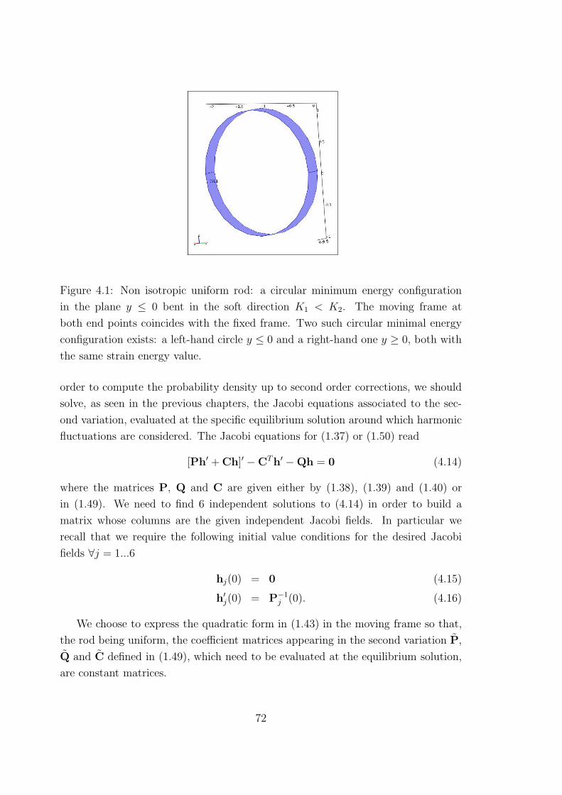
Figure 4.1: Non isotropic uniform rod: a circular minimum energy configuration
in the plane y ≤ 0 bent in the soft direction K1 < K2. The moving frame at
both end points coincides with the fixed frame. Two such circular minimal energy
configuration exists: a left-hand circle y ≤ 0 and a right-hand one y ≥ 0, both with
the same strain energy value.
order to compute the probability density up to second order corrections, we should
solve, as seen in the previous chapters, the Jacobi equations associated to the sec-
ond variation, evaluated at the specific equilibrium solution around which harmonic
fluctuations are considered. The Jacobi equations for (1.37) or (1.50) read
[Ph′ + Ch]′ − CTh′ − Qh = 0 (4.14)
where the matrices P, Q and C are given either by (1.38), (1.39) and (1.40) or
in (1.49). We need to find 6 independent solutions to (4.14) in order to build a
matrix whose columns are the given independent Jacobi fields. In particular we
recall that we require the following initial value conditions for the desired Jacobi
fields ∀j = 1...6
hj(0) = 0 (4.15)
h′j(0) = P−1
j (0). (4.16)
We choose to express the quadratic form in (1.43) in the moving frame so that,
the rod being uniform, the coefficient matrices appearing in the second variation P,
Q and C defined in (1.49), which need to be evaluated at the equilibrium solution,
are constant matrices.
72
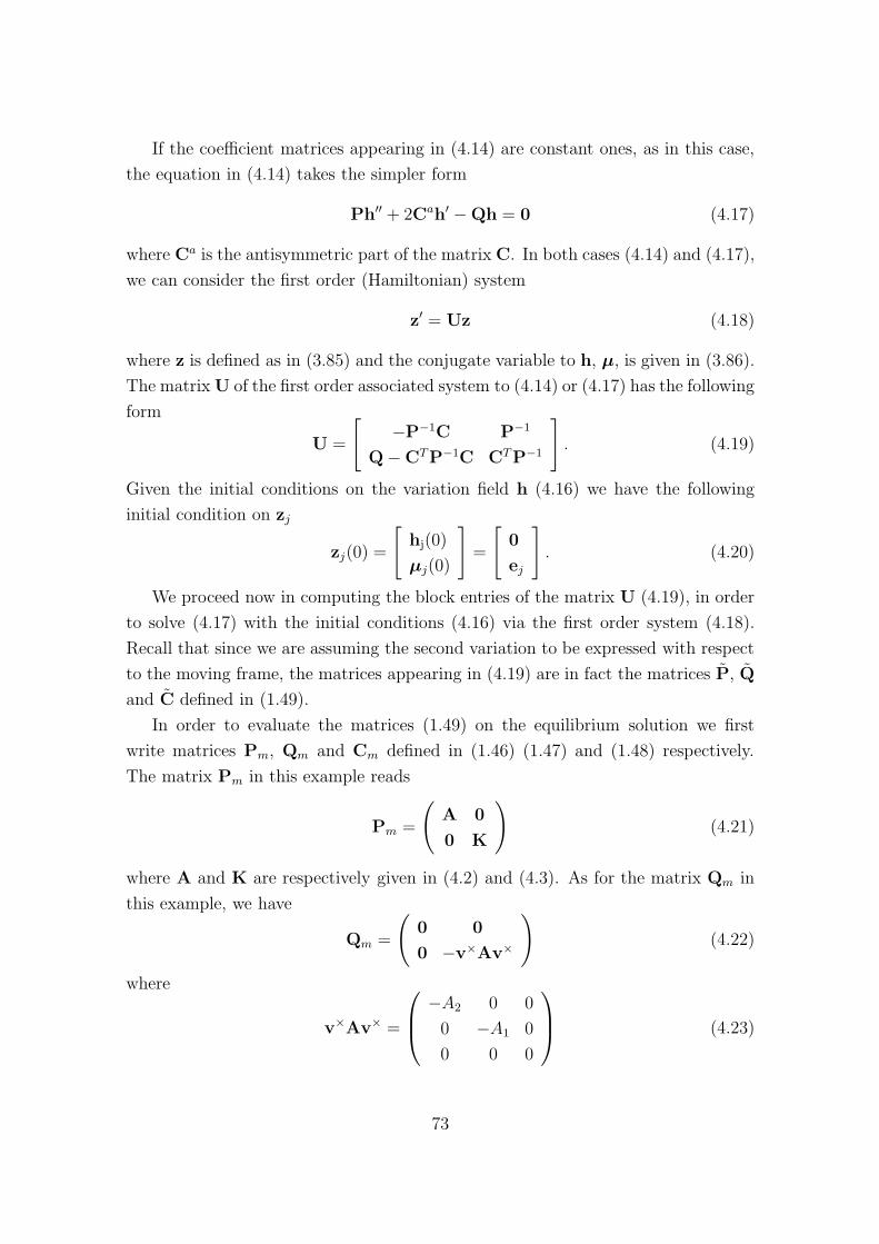
If the coefficient matrices appearing in (4.14) are constant ones, as in this case,
the equation in (4.14) takes the simpler form
Ph′′ + 2Cah′ − Qh = 0 (4.17)
where Ca is the antisymmetric part of the matrix C. In both cases (4.14) and (4.17),
we can consider the first order (Hamiltonian) system
z′ = Uz (4.18)
where z is defined as in (3.85) and the conjugate variable to h, µ, is given in (3.86).
The matrix U of the first order associated system to (4.14) or (4.17) has the following
form
U =
[
−P−1C P−1
Q − CTP−1C CTP−1
]
. (4.19)
Given the initial conditions on the variation field h (4.16) we have the following
initial condition on zj
zj(0) =
[
hj(0)
µj(0)
]
=
[
0
ej
]
. (4.20)
We proceed now in computing the block entries of the matrix U (4.19), in order
to solve (4.17) with the initial conditions (4.16) via the first order system (4.18).
Recall that since we are assuming the second variation to be expressed with respect
to the moving frame, the matrices appearing in (4.19) are in fact the matrices P, Q
and C defined in (1.49).
In order to evaluate the matrices (1.49) on the equilibrium solution we first
write matrices Pm, Qm and Cm defined in (1.46) (1.47) and (1.48) respectively.
The matrix Pm in this example reads
Pm =
(
A 0
0 K
)
(4.21)
where A and K are respectively given in (4.2) and (4.3). As for the matrix Qm in
this example, we have
Qm =
(
0 0
0 −v×Av×
)
(4.22)
where
v×Av× =
−A2 0 0
0 −A1 0
0 0 0
(4.23)
73
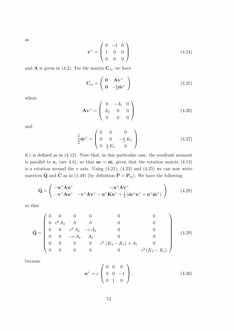
as
v× =
0 −1 0
1 0 0
0 0 0
(4.24)
and A is given in (4.2). For the matrix Cm, we have
Cm =
(
0 Av×
0 −12m×
)
(4.25)
where
Av× =
0 −A1 0
A2 0 0
0 0 0
(4.26)
and
1
2m× =
0 0 0
0 0 − c2K1
0 c2K1 0
, (4.27)
if c is defined as in (4.12). Note that, in this particular case, the resultant moment
is parallel to e1 (see 4.8), so that m = m, given that the rotation matrix (4.13)
is a rotation around the x axis. Using (4.21), (4.23) and (4.25) we can now write
matrices Q and C as in (1.49) (by definition P = Pm). We have the following
Q =
(
−u×Au× −u×Av×
−v×Au× −v×Av× − u×Ku× + 12(m×u× + u×m×)
)
(4.28)
so that
Q =
0 0 0 0 0 0
0 c2 A3 0 0 0 0
0 0 c2 A2 −c A2 0 0
0 0 −c A2 A2 0 0
0 0 0 0 c2 (K3 − K1) + A1 0
0 0 0 0 0 c2 (K2 − K1)
(4.29)
because
u× = c
0 0 0
0 0 −1
0 1 0
, (4.30)
74
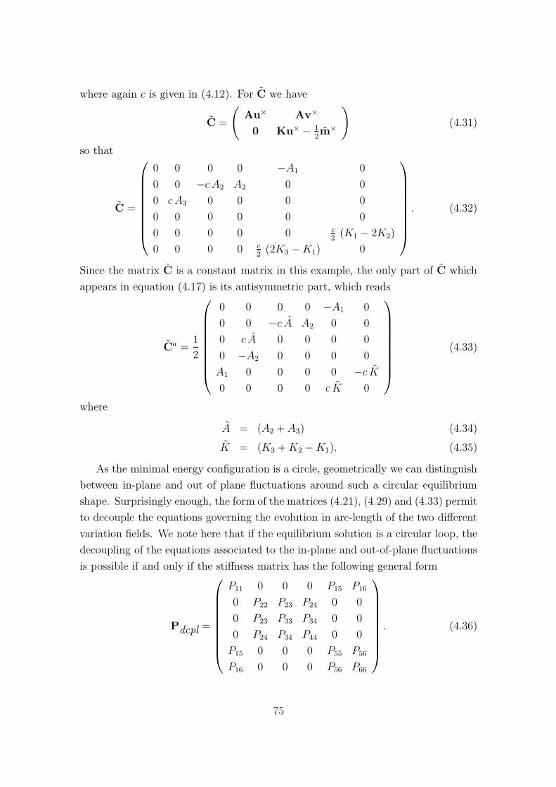
where again c is given in (4.12). For C we have
C =
(
Au× Av×
0 Ku× − 12m×
)
(4.31)
so that
C =
0 0 0 0 −A1 0
0 0 −c A2 A2 0 0
0 c A3 0 0 0 0
0 0 0 0 0 0
0 0 0 0 0 c2
(K1 − 2K2)
0 0 0 0 c2
(2K3 − K1) 0
. (4.32)
Since the matrix C is a constant matrix in this example, the only part of C which
appears in equation (4.17) is its antisymmetric part, which reads
Ca =1
2
0 0 0 0 −A1 0
0 0 −c A A2 0 0
0 c A 0 0 0 0
0 −A2 0 0 0 0
A1 0 0 0 0 −c K
0 0 0 0 c K 0
(4.33)
where
A = (A2 + A3) (4.34)
K = (K3 + K2 − K1). (4.35)
As the minimal energy configuration is a circle, geometrically we can distinguish
between in-plane and out of plane fluctuations around such a circular equilibrium
shape. Surprisingly enough, the form of the matrices (4.21), (4.29) and (4.33) permit
to decouple the equations governing the evolution in arc-length of the two different
variation fields. We note here that if the equilibrium solution is a circular loop, the
decoupling of the equations associated to the in-plane and out-of-plane fluctuations
is possible if and only if the stiffness matrix has the following general form
Pdcpl =
P11 0 0 0 P15 P16
0 P22 P23 P24 0 0
0 P23 P33 P34 0 0
0 P24 P34 P44 0 0
P15 0 0 0 P55 P56
P16 0 0 0 P56 P66
. (4.36)
75
Furthermore assuming that the bending and twist stiffnesses are not coupled implies
P15 = P16 = P24 = P34 = 0, so that the allowed stiffness matrix has the form
Pdcpl2 =
A11 0 0 0 0 0
0 A22 A23 0 0 0
0 A23 A33 0 0 0
0 0 0 K11 0 0
0 0 0 0 K22 K23
0 0 0 0 K23 K33
. (4.37)
In particular, recalling that the circular solution lies in the (y, z) plane with y ≤ 0,
we may define the two vector fields associated with the in-plane fluctuations and
the out-of-plane fluctuations to be respectively
hp =
0
δry
δrz
δΘx
0
0
, hop =
δrx
0
0
0
δΘy
δΘz
. (4.38)
Accordingly, the second variation (1.50) can be written as the sum of two distin-
guished terms
δ2Sstat =1
2
∫ L
0
[
h′T Ph′ + 2h′T Ch + hT Qh]
=1
2
∫ L
0
[
h′Tp P|ph
′p + 2h′T
p C|php + hTpQ|php
]
+1
2
∫ L
0
[
h′TopP|oph
′op + 2h′T
opC|ophop + hTopQ|ophop
]
. (4.39)
where we have removed the s dependency in the coefficient matrices as in this case
they are constant, and
hp = R
δry
δrz
δΘx
(4.40)
hop = R
δrx
δΘy
δΘz
(4.41)
76
where R is given in (4.13). The coefficient matrices in (4.39) read respectively
P|p =
A2 0 0
0 A3 0
0 0 K1
, (4.42)
C|p =
0 −c A2 A2
c A3 0 0
0 0 0
, (4.43)
Q|p =
c2 A3 0 0
0 c2 A2 −c A2
0 −c A2 A2
(4.44)
and
P|op =
A1 0 0
0 K2 0
0 0 K3
, (4.45)
C|op =
0 −A1 0
0 0 − c2(2K2 − K1)
0 c2(2K3 − K1) 0
, (4.46)
Q|op =
0 0 0
0 c2 (K3 − K1) + A1 0
0 0 c2 (K2 − K1)
. (4.47)
where once again c is defined in (4.12). In the probability density function, the
factor due to the harmonic fluctuations around the equilibrium solution can thus be
factorized in two different contributions: one deriving from the planar fluctuations
and one from the off plane fluctuations. We shall compute these contributions
separately.
In plane fluctuations
For the contribution associated with the in-plane fluctuations, we need to solve the
Jacobi equations in (4.17), where the variable h is now the R3 vector (4.40) and
the coefficient matrices are (3 × 3) matrices (4.42), (4.43) and (4.44). We look for
three independent solutions of the projected Jacobi equations, satisfying the initial
77
conditions in (3.82) but where
hj ≡(
hp
)
j
P−1ij ≡
(
P|−1p
)
ij(4.48)
and i, j = 1, 2, 3. For the sake of simplicity of notation in the following we omit all
super and sub scripts, and we assume (4.48). The first order associated Hamiltonian
system is of the form (4.18) where now
µ ≡ P|ph′p + C|php (4.49)
with initial conditions (4.20), if again (4.48) and (4.49) are assumed. The solution
to (4.18) is
z(s) = z(0)eUps (4.50)
where
Up =
0 c −1 1A2
0 0
−c 0 0 0 1A3
0
0 0 0 0 0 1K1
0 0 0 0 c 0
0 0 0 −c 0 0
0 0 0 1 0 0
(4.51)
and c is given in (4.12). The eigenvalues of (4.51) are 0,±i c each of algebraic
multiplicity 2 and geometrical multiplicity 1, so that the solution (4.50) can be
written as
z(s) = MeUBpz(0)F (4.52)
where M = [f1 f2 f3 f4 f5 f6] is the matrix of change of basis between the basis F
of the proper and generalized eigenvectors and the canonical one, UBp is the block
diagonal Jordan form of the matrix Up and z(0)F is the initial value vector expressed
in the basis F . The basis F reads
f1 =
0
1
c
0
0
0
, f2 =
−1c
1
c
0
0
c K1
78
f3 =
1
i
0
0
0
0
, f4 =
−i 2[
A2+c2 K1
A2 c W
]
1c
− 2W
2 c2 K1
W2 i c2 K1
W
−2 i c K1
W
(4.53)
where we have defined
W =
[
1 + c2 K1A2 + A3
A2 A3
]
=
[
1 +
(
2π
L
)2
K1
(
1
A2+
1
A3
)
]
(4.54)
and f1,2 are the proper/generalized eigenvectors associated with the eigenvalue 0, f3,4
are the proper/generalized eigenvectors associated with the eigenvalue ic (of course
f5 = f3, f6 = f4). Note that W as defined in (4.54) is dimensionless, as ∀i = 1, 2, 3
[Ai] =[E]
[l]⇒
[
A2 + A3
A2 A3
]
= [l]/[E]
[Ki] = [E][l] ⇒ [c2 K1] = [E]/[l] (4.55)
where E stands for energy and l for length. The general solution to (4.17) in this
case can thus be written as
h(s) = α
0
1
c
+ β
−1c
1
c
+ s
0
1
c
+ γ eics
1
i
0
+ δ eics
−i 2[
A2+c2 K1
A2 c W
]
1c
− 2W
+ s
1
i
0
+ ǫ e−ics
1
−i
0
+ η e−ics
i 2[
A2+c2 K1
A2 c W
]
1c
− 2W
+ s
1
−i
0
(4.56)
where the constants α, β, γ, δ, ǫ, η depend on the initial conditions imposed. In con-
clusion, the three independent solutions of (4.17) satisfying (4.16) with the assump-
tion (4.48) are:
h1(s) =
[
A2 W (cs cos cs − sin cs) + 2 c2 K1 sin cs
2 A2 c3 K1
2 (1 − cos cs) − W cs sin cs
2 c3 K1
1 − cos cs
c2 K1
]T
79
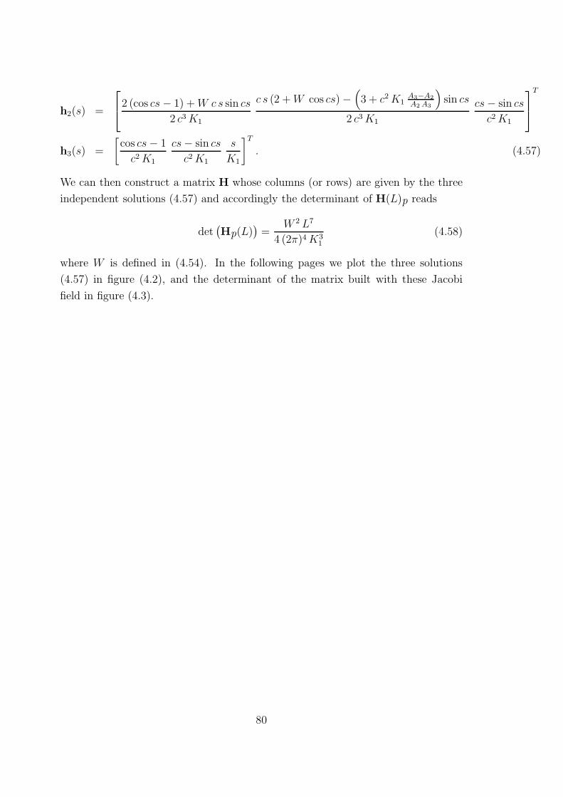
h2(s) =
2 (cos cs − 1) + W c s sin cs
2 c3 K1
c s (2 + W cos cs) −(
3 + c2 K1A3−A2
A2 A3
)
sin cs
2 c3 K1
cs − sin cs
c2 K1
T
h3(s) =
[
cos cs − 1
c2 K1
cs − sin cs
c2 K1
s
K1
]T
. (4.57)
We can then construct a matrix H whose columns (or rows) are given by the three
independent solutions (4.57) and accordingly the determinant of H(L)p reads
det(
Hp(L))
=W 2 L7
4 (2π)4 K31
(4.58)
where W is defined in (4.54). In the following pages we plot the three solutions
(4.57) in figure (4.2), and the determinant of the matrix built with these Jacobi
field in figure (4.3).
80
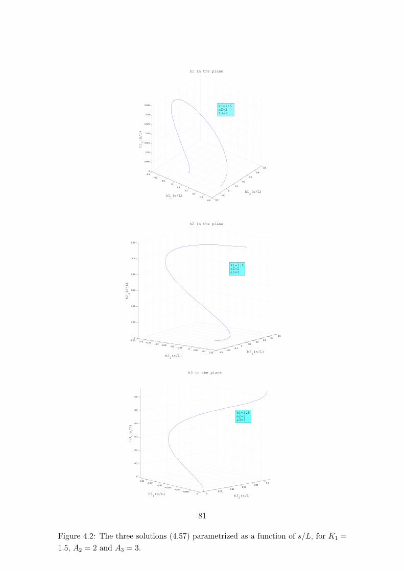
−0.3
−0.2
−0.1
0
0.1
0.2
0.3
0.4
0.5 −0.2
−0.1
0
0.1
0.2
0.3
0.4
0.5
0
0.005
0.01
0.015
0.02
0.025
0.03
0.035
h12(s/L)
h1 in the plane
h11(s/L)
h13(s/L)
k1=1/5a2=2a3=3
−0.35−0.3
−0.25−0.2
−0.15−0.1
−0.050
0.050.1
0.15 −0.3−0.2
−0.10
0.10.2
0.30.4
0.50
0.02
0.04
0.06
0.08
0.1
0.12
h22(s/L)
h2 in the plane
h21(s/L)
h23(s/L)
k1=1.5a2=2a3=3
−0.03−0.025
−0.02−0.015
−0.01−0.005
0 00.02
0.040.06
0.080.1
0
0.1
0.2
0.3
0.4
0.5
0.6
h32(s/L)
h3 in the plane
h31(s/L)
h33(s/L)
k1=1.5a2=2a3=3
Figure 4.2: The three solutions (4.57) parametrized as a function of s/L, for K1 =
1.5, A2 = 2 and A3 = 3.
81
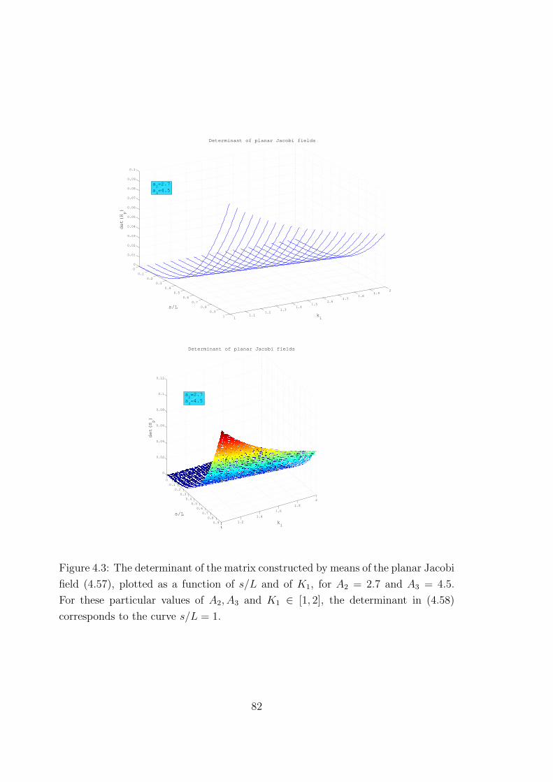
0
0.1
0.2
0.3
0.4
0.5
0.6
0.7
0.8
0.9
1 11.1
1.21.3
1.41.5
1.61.7
1.81.9
2
0
0.01
0.02
0.03
0.04
0.05
0.06
0.07
0.08
0.09
0.1
k1
Determinant of planar Jacobi fields
s/L
det(Hp)
a2=2.7
a3=4.5
0
0.1
0.2
0.3
0.4
0.5
0.6
0.7
0.8
0.9
11
1.2
1.4
1.6
1.8
2
0
0.02
0.04
0.06
0.08
0.1
0.12
k1
Determinant of planar Jacobi fields
s/L
det(Hp)
a2=2.7
a3=4.5
Figure 4.3: The determinant of the matrix constructed by means of the planar Jacobi
field (4.57), plotted as a function of s/L and of K1, for A2 = 2.7 and A3 = 4.5.
For these particular values of A2, A3 and K1 ∈ [1, 2], the determinant in (4.58)
corresponds to the curve s/L = 1.
82
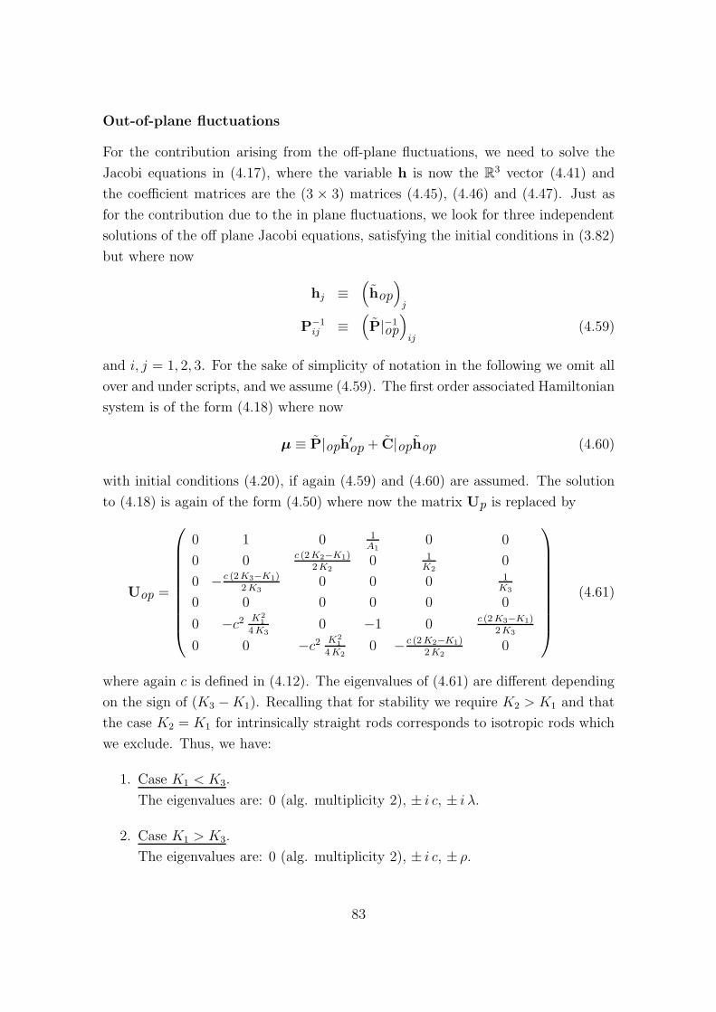
Out-of-plane fluctuations
For the contribution arising from the off-plane fluctuations, we need to solve the
Jacobi equations in (4.17), where the variable h is now the R3 vector (4.41) and
the coefficient matrices are the (3 × 3) matrices (4.45), (4.46) and (4.47). Just as
for the contribution due to the in plane fluctuations, we look for three independent
solutions of the off plane Jacobi equations, satisfying the initial conditions in (3.82)
but where now
hj ≡(
hop
)
j
P−1ij ≡
(
P|−1op
)
ij(4.59)
and i, j = 1, 2, 3. For the sake of simplicity of notation in the following we omit all
over and under scripts, and we assume (4.59). The first order associated Hamiltonian
system is of the form (4.18) where now
µ ≡ P|oph′op + C|ophop (4.60)
with initial conditions (4.20), if again (4.59) and (4.60) are assumed. The solution
to (4.18) is again of the form (4.50) where now the matrix Up is replaced by
Uop =
0 1 0 1A1
0 0
0 0 c (2 K2−K1)2 K2
0 1K2
0
0 − c (2 K3−K1)2 K3
0 0 0 1K3
0 0 0 0 0 0
0 −c2 K21
4 K30 −1 0 c (2 K3−K1)
2 K3
0 0 −c2 K21
4 K20 − c (2 K2−K1)
2 K20
(4.61)
where again c is defined in (4.12). The eigenvalues of (4.61) are different depending
on the sign of (K3 − K1). Recalling that for stability we require K2 > K1 and that
the case K2 = K1 for intrinsically straight rods corresponds to isotropic rods which
we exclude. Thus, we have:
1. Case K1 < K3.
The eigenvalues are: 0 (alg. multiplicity 2), ± i c, ± i λ.
2. Case K1 > K3.
The eigenvalues are: 0 (alg. multiplicity 2), ± i c, ± ρ.
83
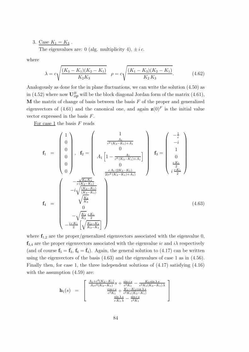
3. Case K1 = K3 .
The eigenvalues are: 0 (alg. multiplicity 4), ± i c.
where
λ = c
√
(K3 − K1)(K2 − K1)
K2K3
ρ = c
√
(K1 − K3)(K2 − K1)
K2 K3
. (4.62)
Analogously as done for the in plane fluctuations, we can write the solution (4.50) as
in (4.52) where now UBop will be the block diagonal Jordan form of the matrix (4.61),
M the matrix of change of basis between the basis F of the proper and generalized
eigenvectors of (4.61) and the canonical one, and again z(0)F is the initial value
vector expressed in the basis F .
For case 1 the basis F reads
f1 =
1
0
0
0
0
0
, f2 =
1A1
c2 (K3−K1)+A1
0
A1
[
1 − A1
c2 (K3−K1)+A1
]
0c A1 (2K3−K1)
2(c2 (K3−K1)+A1)
f3 =
−1c
−i
1
0c K1
2
i c K1
2
f4 =
−√
K2 K3
c (K3−K1)
−i√
(K2−K1)(K3−K1)√
K2
K3
0
−√
K2
K3
c K1
2
− i c K1
2
[√
K2−K1
K3−K1
]
(4.63)
where f1,2 are the proper/generalized eigenvectors associated with the eigenvalue 0,
f3,4 are the proper eigenvectors associated with the eigenvalue ic and iλ respectively
(and of course f5 = f3, f6 = f4). Again, the general solution to (4.17) can be written
using the eigenvectors of the basis (4.63) and the eigenvalues of case 1 as in (4.56).
Finally then, for case 1, the three independent solutions of (4.17) satisfying (4.16)
with the assumption (4.59) are:
h1(s) =
A1+c2(K3−K1)A1c2(K3−K1)
s + sin c sc3K1
− K3 sin λ sc2K1(K3−K1) λ
cos c sc2K1
+ K1−K3 cos λ sc2K1(K3−K1)
sinλ sc K1 λ
− sin c sc2K1
84
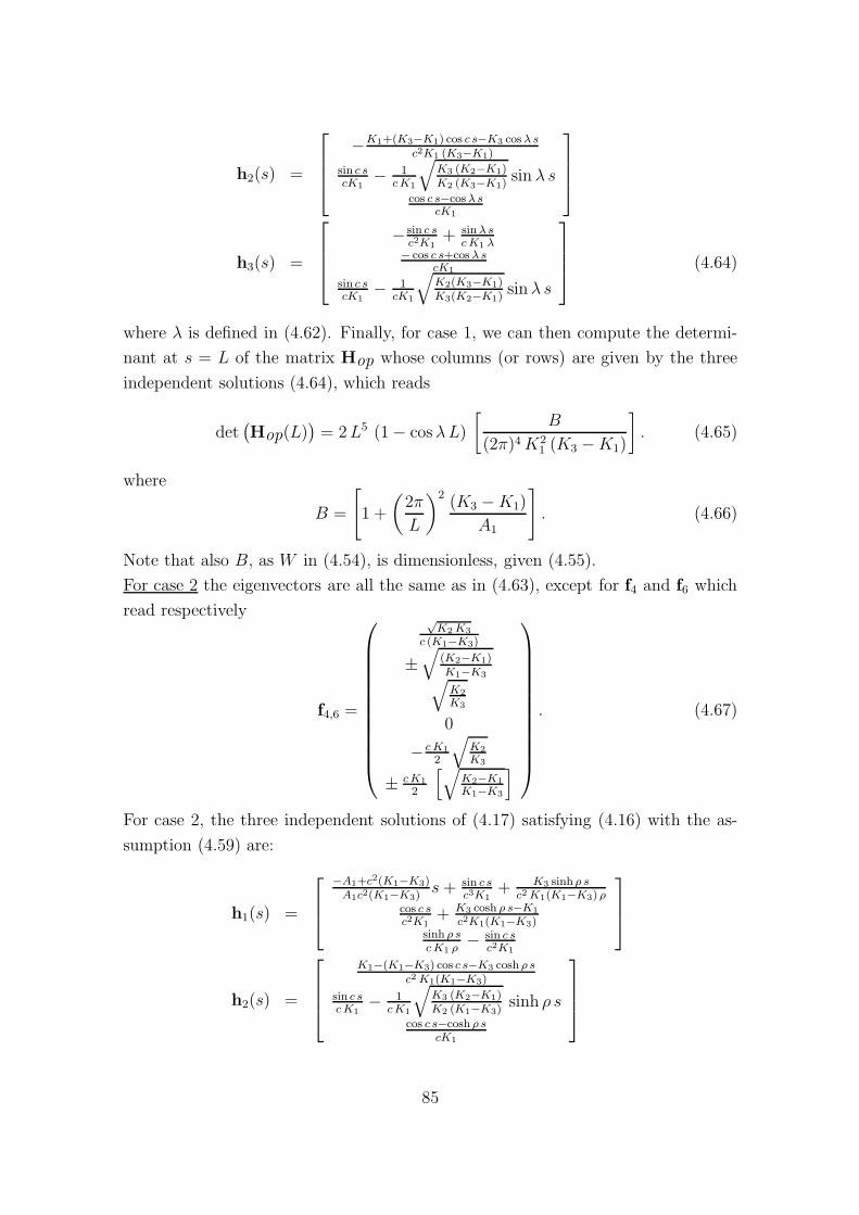
h2(s) =
−K1+(K3−K1) cos c s−K3 cos λ sc2K1 (K3−K1)
sin c scK1
− 1c K1
√
K3 (K2−K1)K2 (K3−K1)
sin λ scos c s−cos λ s
cK1
h3(s) =
− sin c sc2K1
+ sin λsc K1 λ
− cos c s+cos λ scK1
sin c scK1
− 1cK1
√
K2(K3−K1)K3(K2−K1)
sin λ s
(4.64)
where λ is defined in (4.62). Finally, for case 1, we can then compute the determi-
nant at s = L of the matrix Hop whose columns (or rows) are given by the three
independent solutions (4.64), which reads
det(
Hop(L))
= 2 L5 (1 − cos λ L)
[
B
(2π)4 K21 (K3 − K1)
]
. (4.65)
where
B =
[
1 +
(
2π
L
)2(K3 − K1)
A1
]
. (4.66)
Note that also B, as W in (4.54), is dimensionless, given (4.55).
For case 2 the eigenvectors are all the same as in (4.63), except for f4 and f6 which
read respectively
f4,6 =
√K2 K3
c (K1−K3)
±√
(K2−K1)K1−K3
√
K2
K3
0
− c K1
2
√
K2
K3
± c K1
2
[√
K2−K1
K1−K3
]
. (4.67)
For case 2, the three independent solutions of (4.17) satisfying (4.16) with the as-
sumption (4.59) are:
h1(s) =
−A1+c2(K1−K3)A1c2(K1−K3)
s + sin c sc3K1
+ K3 sinh ρ sc2 K1(K1−K3) ρ
cos c sc2K1
+ K3 cosh ρ s−K1
c2K1(K1−K3)sinh ρ sc K1 ρ
− sin c sc2K1
h2(s) =
K1−(K1−K3) cos c s−K3 cosh ρ sc2 K1(K1−K3)
sin c sc K1
− 1c K1
√
K3 (K2−K1)K2 (K1−K3)
sinh ρ scos c s−cosh ρ s
cK1
85
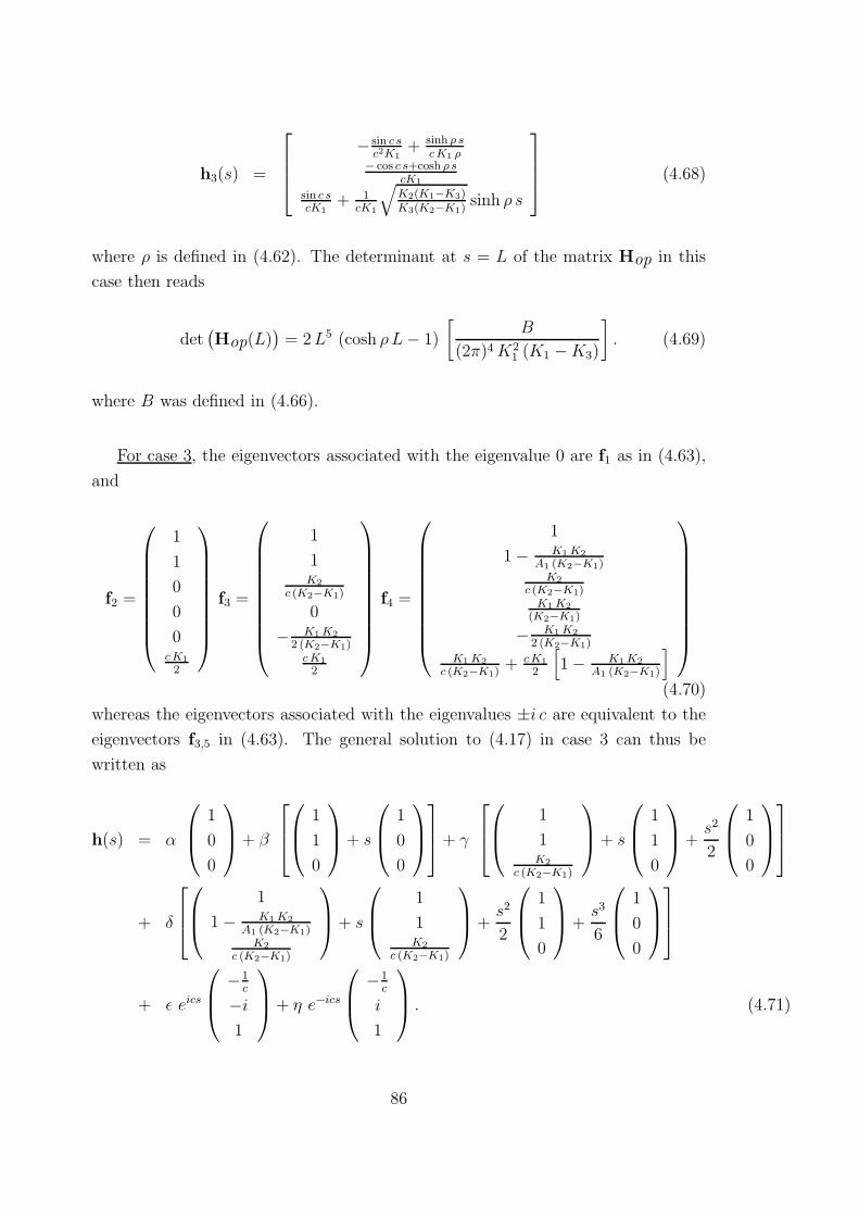
h3(s) =
− sin c sc2K1
+ sinh ρ sc K1 ρ
− cos c s+cosh ρ scK1
sin c scK1
+ 1cK1
√
K2(K1−K3)K3(K2−K1)
sinh ρ s
(4.68)
where ρ is defined in (4.62). The determinant at s = L of the matrix Hop in this
case then reads
det(
Hop(L))
= 2 L5 (cosh ρ L − 1)
[
B
(2π)4 K21 (K1 − K3)
]
. (4.69)
where B was defined in (4.66).
For case 3, the eigenvectors associated with the eigenvalue 0 are f1 as in (4.63),
and
f2 =
1
1
0
0
0c K1
2
f3 =
1
1K2
c (K2−K1)
0
− K1 K2
2 (K2−K1)c K1
2
f4 =
1
1 − K1 K2
A1 (K2−K1)K2
c (K2−K1)K1 K2
(K2−K1)
− K1 K2
2 (K2−K1)
K1 K2
c (K2−K1)+ c K1
2
[
1 − K1 K2
A1 (K2−K1)
]
(4.70)
whereas the eigenvectors associated with the eigenvalues ±i c are equivalent to the
eigenvectors f3,5 in (4.63). The general solution to (4.17) in case 3 can thus be
written as
h(s) = α
1
0
0
+ β
1
1
0
+ s
1
0
0
+ γ
1
1K2
c (K2−K1)
+ s
1
1
0
+
s2
2
1
0
0
+ δ
1
1 − K1 K2
A1 (K2−K1)K2
c (K2−K1)
+ s
1
1K2
c (K2−K1)
+
s2
2
1
1
0
+
s3
6
1
0
0
+ ǫ eics
−1c
−i
1
+ η e−ics
−1c
i
1
. (4.71)
86
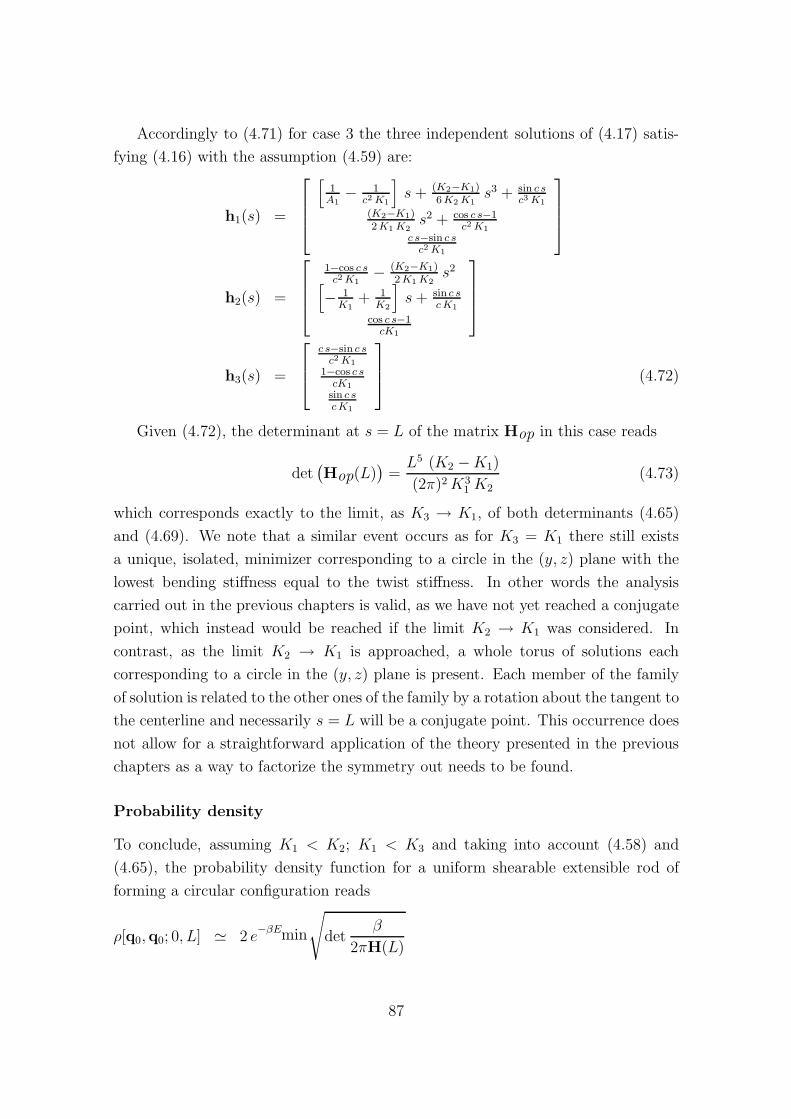
Accordingly to (4.71) for case 3 the three independent solutions of (4.17) satis-
fying (4.16) with the assumption (4.59) are:
h1(s) =
[
1A1
− 1c2 K1
]
s + (K2−K1)6 K2 K1
s3 + sin c sc3 K1
(K2−K1)2 K1 K2
s2 + cos c s−1c2 K1
c s−sin c sc2 K1
h2(s) =
1−cos c sc2 K1
− (K2−K1)2 K1 K2
s2
[
− 1K1
+ 1K2
]
s + sin c sc K1
cos c s−1cK1
h3(s) =
c s−sin c sc2 K1
1−cos c scK1
sin c sc K1
(4.72)
Given (4.72), the determinant at s = L of the matrix Hop in this case reads
det(
Hop(L))
=L5 (K2 − K1)
(2π)2 K31 K2
(4.73)
which corresponds exactly to the limit, as K3 → K1, of both determinants (4.65)
and (4.69). We note that a similar event occurs as for K3 = K1 there still exists
a unique, isolated, minimizer corresponding to a circle in the (y, z) plane with the
lowest bending stiffness equal to the twist stiffness. In other words the analysis
carried out in the previous chapters is valid, as we have not yet reached a conjugate
point, which instead would be reached if the limit K2 → K1 was considered. In
contrast, as the limit K2 → K1 is approached, a whole torus of solutions each
corresponding to a circle in the (y, z) plane is present. Each member of the family
of solution is related to the other ones of the family by a rotation about the tangent to
the centerline and necessarily s = L will be a conjugate point. This occurrence does
not allow for a straightforward application of the theory presented in the previous
chapters as a way to factorize the symmetry out needs to be found.
Probability density
To conclude, assuming K1 < K2; K1 < K3 and taking into account (4.58) and
(4.65), the probability density function for a uniform shearable extensible rod of
forming a circular configuration reads
ρ[q0,q0; 0, L] ≃ 2 e−βEmin
√
detβ
2πH(L)
87
= 2 e−2βπ2K1
L
[
(
β
2π
)3/2√
4 (2π)4K31
L7W 2
]
p
[
(
β
2π
)3/2√
(2π)4K21 (K3 − K1)
L5B(1 − cos λL)
]
op
= 2 e−2βπ2K1
L4π β3
L6 W
[√
K51 (K3 − K1)
B (1 − cos λ L)
]
(4.74)
where W was defined in (4.54), B in (4.66) and λ in (4.62). Recalling that W in
(4.54) and B in (4.66) are dimensionless, the whole correction term has dimensions
[correction] =1
[E]3[L]6
√
[E]6[L]6 =1
[L]3. (4.75)
Defining
Lp = βK1, L = L/Lp (4.76)
the formula (4.74) becomes
ρ[q0,q0; 0, L] ≃ 2 e−2π2
L4π
L6 A
[√
γ − 1
B (1 − cos α)
]
1
L3p
(4.77)
where
α = 2π
√
(K3 − K1) (K2 − K1)
K2 K3(4.78)
and
A =
[
1 + 4π2
(
1
Sh2
+1
Ex
)
1
L2
]
B =
[
1 + 4π2
(
(γ − 1)
Sh1
)
1
L2
]
(4.79)
with
Sh1 = β2 A1 K1, Sh2 = β2 A2 K1, Ex = β2 A3 K1, γ =K3
K1. (4.80)
Furthermore, we could consider the limit as Ai are sent to infinity of the probability
density function in (4.77) to get
ρ[q0,q0; 0, L]Lim ≃ 2 e−2π2
L4π
L6
[√
(K3 − K1)
K1 (1 − cos α)
]
1
L3p
(4.81)
In the limiting case where K1 = K3, taking into account (4.58) and (4.73), the
probability density function is given by
ρ[q0,q0; 0, L] ≃ 2 e−βEmin
√
detβ
2πH(L)
88
= 2 e−2βπ2K1
L
[
(
β
2π
)3/2√
4 (2π)4K31
L7 W 2
]
p
[
(
β
2π
)3/2√
(2π)2K31 K2
L5(K2 − K1)
]
op
= 2 e−2βπ2K1
L2 β3 K3
1
L6 W
[√
K2
(K2 − K1)
]
(4.82)
where again W is defined in (4.54). Making use of the definitions (4.76) yields to
ρ[q0,q0; 0, L] ≃ 2 e−2π2
L2
L6 W
[√
K2
(K2 − K1)
]
1
L3p
(4.83)
and again taking the limit as the shears are sent to infinity leads to
ρ[q0,q0; 0, L]lim ≃ 2 e−2π2
L2
L6
[√
K2
(K2 − K1)
]
1
L3p
(4.84)
which in fact corresponds to the limit of (4.81) as K3 approaches K1.
4.2 Unshearable inextensible rods
As we have already discussed in Chapter 1 and 3, inextensible and unshearable rods
are constrained to have their length fixed and not to deform along an orthogonal
plane to the rod’s cross section. For these rods the shear stiffnesses rise to infinity,
indicating the prohibition for the rod to explore configurations in which deformations
associated with the shear stiffnesses are present and the director d3(s) corresponds
to the tangent vector to the centerline, as in (1.52). In any configuration of an
inextensible and unshearable rod the parameter s is arc-length, so that the vector
V defined in (1.13) is identically equal to zero. The constraint (1.52) is an integral
constraint, as is clear in (1.54), which complicates matters as far as the derivations
in Chapter 2 and 3 are concerned. Moreover, our ultimate aim being the modeling
of DNA, it is not inappropriate to consider instead of a constrained rod, a slightly
shearable and extensible one and define the inextensible unshearable rod to coincide
with the limit of the unconstrained rod as the shear stiffnesses approach infinity.
Accordingly, we scale the stiffness matrix by an arbitrary factor ω > 0, so that
the stiffness matrix in the moving frame reads
P =
(
A/ω 0
0 K
)
(4.85)
89
where the matrices A and K are respectively defined in (4.2) and (4.3). The con-
strained system of an inextensible and unshearable rod, corresponds to the limit in
which, for finite shears, ω → 0 and P−1 has a finite limit:
P−1 → P−1inext
=
(
0 0
0 K−1
)
. (4.86)
4.2.1 A circular loop
As in the shearable extensible case, the boundary conditions for a circular loop are
(4.6). We will again assume the circular loop to be stable and to be in the (y, z)
plane, so that the condition K1 < K2 is forced. In particular, we will again assume
y ≤ 0. The strains are given in (4.8) and (4.9). The centerline and the director
frame of the circular loop are defined in (4.10) and (4.11), whereas the rotation
matrix relating the fixed frame to the moving frame is given in (4.13). According to
Chapter 3, we will directly proceed to considering the first order Hamiltonian system
(3.83), where the variable z is defined in (3.85). In this specific example, the limiting
matrix (3.91) allows again for a decoupling between the evolution equations along
the rod of the in-plane and off-plane fluctuations and their respective conjugate
momenta (3.86). Therefore we shall keep in mind the definitions (4.38) and imagine
an analogous definition for the in-plane and out-of-plane conjugate momenta: we
will then need to solve two different equations of the form
z′ = [JS]inext
z = Uinext z (4.87)
where in each case the variable z ∈ R6 and the matrix Uinext = [JS]inext will be given
either by, for the in-plane fluctuations,
Uinext
p = limω→0
0 c −1 ωA2
0 0
−c 0 0 0 ωA3
0
0 0 0 0 0 1K1
0 0 0 0 c 0
0 0 0 −c 0 0
0 0 0 1 0 0
=
0 c −1 0 0 0
−c 0 0 0 0 0
0 0 0 0 0 1K1
0 0 0 0 c 0
0 0 0 −c 0 0
0 0 0 1 0 0
(4.88)
90
or by, for the out-of-plane fluctuations,
Uinext
op = limω→0
0 1 0 ωA1
0 0
0 0 c (2 K2−K1)2 K2
0 1K2
0
0 − c (2 K3−K1)2 K3
0 0 0 1K3
0 0 0 0 0 0
0 −c2 K21
4 K30 −1 0 c (2 K3−K1)
2 K3
0 0 −c2 K21
4 K20 − c (2 K2−K1)
2 K20
=
0 1 0 0 0 0
0 0 c (2 K2−K1)2 K2
0 1K2
0
0 − c (2 K3−K1)2 K3
0 0 0 1K3
0 0 0 0 0 0
0 −c2 K21
4 K30 −1 0 c (2 K3−K1)
2 K3
0 0 −c2 K21
4 K20 − c (2 K2−K1)
2 K20
. (4.89)
In particular we can conclude that the analysis carried out in the previous sec-
tion concerning the eigenvectors and proper/generalized eigenvectors of each of the
matrices (4.51) and (4.61), is enough to complete the spectral analysis of the ma-
trices given in (4.88) and (4.89). In fact the parameter ω can be thought of as a
perturbation parameter, so that the unperturbed system would correspond to the
inextensible/unshearable system, whereas the perturbed system would correspond
to the extensible/shearable system. In this sense we could write
Up(ω) = Uinext
p + ωU1p
Uop(ω) = Uinext
op + ωU1op (4.90)
where Up(ω), Uop(ω) correspond to matrices (4.51) and (4.61) once the scaling
(4.85) is introduced; matrices Uinext
p and Uinext
op are given in (4.88) and (4.89); and
U1p, U1
op are constant matrices. Even with the scaling (4.85), the eigenvalues of
(4.51) and (4.61) do not depend on ω, so that they will be identical to the eigenval-
ues of their correspondending zero order or unperturbed matrices (4.88) and (4.89).
The proper and generalized eigenvectors of (4.88) and (4.89) in turn will just co-
incide to the limit, as the perturbation parameter approaches zero, of the proper
and generalized eigenvectors of the scaled version of matrices (4.51) and (4.61). The
only substantial difference is that the Jacobi equations (4.17) do not have an ap-
propriate limit in the unperturbed system, so that only the associated first order
Hamiltonian equations (4.87) can be considered and solved. In the following, as for
91
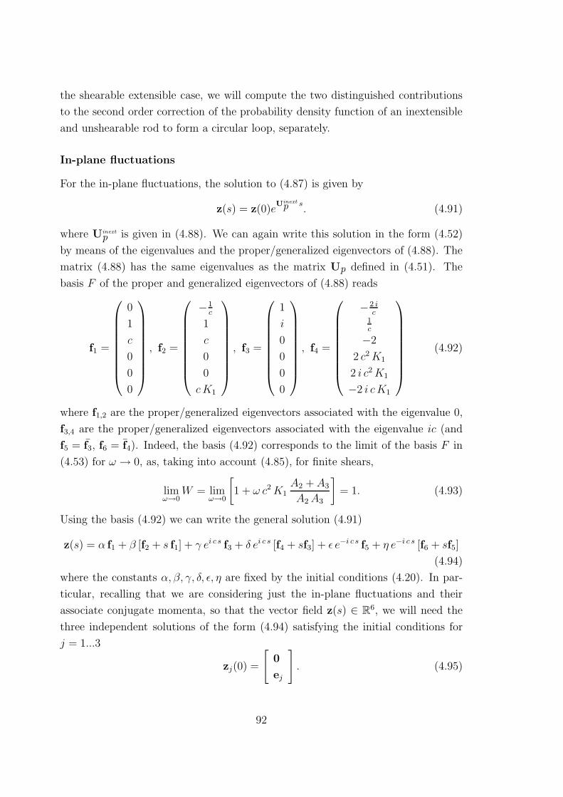
the shearable extensible case, we will compute the two distinguished contributions
to the second order correction of the probability density function of an inextensible
and unshearable rod to form a circular loop, separately.
In-plane fluctuations
For the in-plane fluctuations, the solution to (4.87) is given by
z(s) = z(0)eUinext
p s. (4.91)
where Uinext
p is given in (4.88). We can again write this solution in the form (4.52)
by means of the eigenvalues and the proper/generalized eigenvectors of (4.88). The
matrix (4.88) has the same eigenvalues as the matrix Up defined in (4.51). The
basis F of the proper and generalized eigenvectors of (4.88) reads
f1 =
0
1
c
0
0
0
, f2 =
−1c
1
c
0
0
c K1
, f3 =
1
i
0
0
0
0
, f4 =
−2 ic
1c
−2
2 c2 K1
2 i c2 K1
−2 i c K1
(4.92)
where f1,2 are the proper/generalized eigenvectors associated with the eigenvalue 0,
f3,4 are the proper/generalized eigenvectors associated with the eigenvalue ic (and
f5 = f3, f6 = f4). Indeed, the basis (4.92) corresponds to the limit of the basis F in
(4.53) for ω → 0, as, taking into account (4.85), for finite shears,
limω→0
W = limω→0
[
1 + ω c2 K1A2 + A3
A2 A3
]
= 1. (4.93)
Using the basis (4.92) we can write the general solution (4.91)
z(s) = α f1 + β [f2 + s f1] + γ ei c s f3 + δ ei c s [f4 + sf3] + ǫ e−i c s f5 + η e−i c s [f6 + sf5]
(4.94)
where the constants α, β, γ, δ, ǫ, η are fixed by the initial conditions (4.20). In par-
ticular, recalling that we are considering just the in-plane fluctuations and their
associate conjugate momenta, so that the vector field z(s) ∈ R6, we will need the
three independent solutions of the form (4.94) satisfying the initial conditions for
j = 1...3
zj(0) =
[
0
ej
]
. (4.95)
92
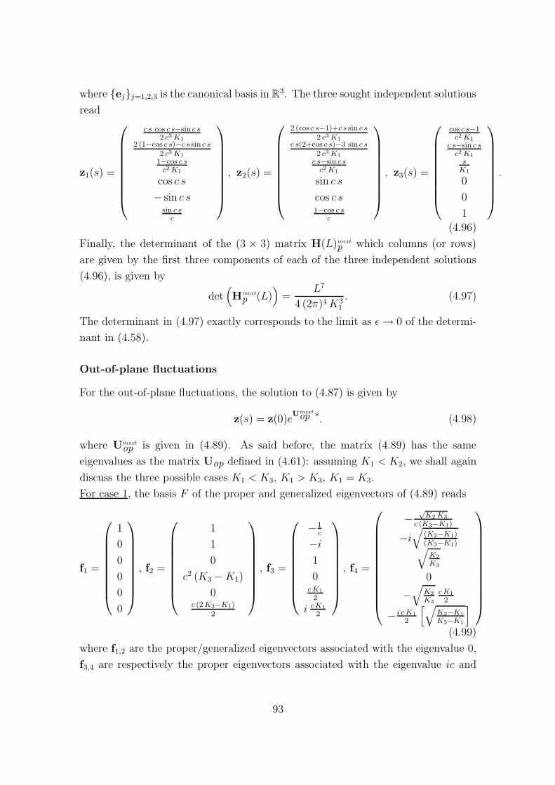
where {ej}j=1,2,3 is the canonical basis in R3. The three sought independent solutions
read
z1(s) =
c s cos c s−sin c s2 c3 K1
2 (1−cos c s)−c s sin c s2 c3 K1
1−cos c sc2 K1
cos c s
− sin c ssin c s
c
, z2(s) =
2 (cos c s−1)+c s sin c s2 c3 K1
c s(2+cos c s)−3 sin c s2 c3 K1
c s−sin c sc2 K1
sin c s
cos c s1−cos c s
c
, z3(s) =
cos c s−1c2 K1
c s−sin c sc2 K1
sK1
0
0
1
.
(4.96)
Finally, the determinant of the (3 × 3) matrix H(L)inext
p which columns (or rows)
are given by the first three components of each of the three independent solutions
(4.96), is given by
det(
Hinext
p (L))
=L7
4 (2π)4 K31
. (4.97)
The determinant in (4.97) exactly corresponds to the limit as ǫ → 0 of the determi-
nant in (4.58).
Out-of-plane fluctuations
For the out-of-plane fluctuations, the solution to (4.87) is given by
z(s) = z(0)eUinext
op s. (4.98)
where Uinext
op is given in (4.89). As said before, the matrix (4.89) has the same
eigenvalues as the matrix Uop defined in (4.61): assuming K1 < K2, we shall again
discuss the three possible cases K1 < K3, K1 > K3, K1 = K3.
For case 1, the basis F of the proper and generalized eigenvectors of (4.89) reads
f1 =
1
0
0
0
0
0
, f2 =
1
1
0
c2 (K3 − K1)
0c (2 K3−K1)
2
, f3 =
−1c
−i
1
0c K1
2
i c K1
2
, f4 =
−√
K2 K3
c (K3−K1)
−i√
(K2−K1)(K3−K1)√
K2
K3
0
−√
K2
K3
c K1
2
− i c K1
2
[√
K2−K1
K3−K1
]
(4.99)
where f1,2 are the proper/generalized eigenvectors associated with the eigenvalue 0,
f3,4 are respectively the proper eigenvectors associated with the eigenvalue ic and
93
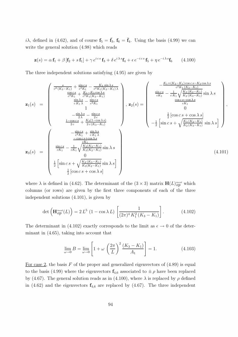
iλ, defined in (4.62), and of course f5 = f3, f6 = f4. Using the basis (4.99) we can
write the general solution (4.98) which reads
z(s) = α f1 + β [f2 + s f1] + γ ei c s f3 + δ ei λ sf4 + ǫ e−i c s f5 + η e−i λ sf6 (4.100)
The three independent solutions satisfying (4.95) are given by
z1(s) =
sc2 (K3−K1)
+ sin c sc3K1
− K3 sinλ sc2K1(K3−K1) λ
cos c sc2K1
+ K1−K3 cos λ sc2K1(K3−K1)
sin λ sc K1 λ
− sin c sc2K1
1
− sin λs2 λ
− sin c s2 c
1−cos c s2 c
+ K3(1−cos λ s)2 c (K3−K1)
, z2(s) =
−K1+(K3−K1) cos c s−K3 cos λ sc2K1 (K3−K1)
sin c scK1
− 1c K1
√
K3 (K2−K1)K2 (K3−K1)
sin λ scos c s−cos λ s
cK1
012[cos c s + cos λ s]
−12
[
sin c s +√
K3 (K2−K1)K2 (K3−K1)
sin λ s]
,
z3(s) =
− sin c sc2K1
+ sinλ sc K1 λ
− cos c s+cos λ scK1
sin c scK1
− 1cK1
√
K2(K3−K1)K3(K2−K1)
sin λ s
0
12
[
sin c s +√
K2 (K3−K1)K3(K2−K1)
sin λ s]
12[cos c s + cos λ s]
(4.101)
where λ is defined in (4.62). The determinant of the (3 × 3) matrix H(L)inext
op which
columns (or rows) are given by the first three components of each of the three
independent solutions (4.101), is given by
det(
Hinext
op (L))
= 2 L5 (1 − cos λ L)
[
1
(2π)4 K21 (K3 − K1)
]
. (4.102)
The determinant in (4.102) exactly corresponds to the limit as ǫ → 0 of the deter-
minant in (4.65), taking into account that
limω→0
B = limω→0
[
1 + ω
(
2π
L
)2(K3 − K1)
A1
]
= 1. (4.103)
For case 2, the basis F of the proper and generalized eigenvectors of (4.89) is equal
to the basis (4.99) where the eigenvectors f4,6 associated to ± ρ have been replaced
by (4.67). The general solution reads as in (4.100), where λ is replaced by ρ defined
in (4.62) and the eigenvectors f4,6 are replaced by (4.67). The three independent
94
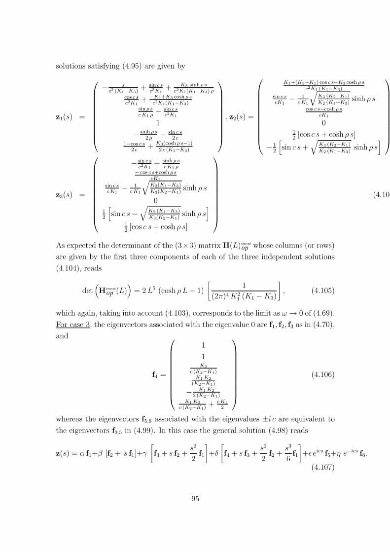
solutions satisfying (4.95) are given by
z1(s) =
− sc2 (K1−K3)
+ sin c sc3K1
+ K3 sinh ρ sc2K1(K1−K3) ρ
cos c sc2K1
+ −K1+K3 cosh ρ sc2K1(K1−K3)
sin ρ sc K1 ρ
− sin c sc2K1
1
− sinh ρ s2 ρ
− sin c s2 c
1−cos c s2 c
+ K3(cosh ρ s−1)2 c (K1−K3)
, z2(s) =
K1+(K3−K1) cos c s−K3 cosh ρ sc2K1 (K1−K3)
sin c scK1
− 1c K1
√
K3 (K2−K1)K2 (K1−K3)
sinh ρ scos c s−cosh ρ s
cK1
012[cos c s + cosh ρ s]
−12
[
sin c s +√
K3 (K2−K1)K2 (K1−K3)
sinh ρ s]
z3(s) =
− sin c sc2K1
+ sinh ρ sc K1 ρ
− cos c s+cosh ρ scK1
sin c sc K1
− 1c K1
√
K2(K1−K3)K3(K2−K1)
sinh ρ s
0
12
[
sin c s −√
K2 (K1−K3)K3(K2−K1)
sinh ρ s]
12[cos c s + cosh ρ s]
(4.104)
As expected the determinant of the (3×3) matrix H(L)inext
op whose columns (or rows)
are given by the first three components of each of the three independent solutions
(4.104), reads
det(
Hinext
op (L))
= 2 L5 (cosh ρ L − 1)
[
1
(2π)4 K21 (K1 − K3)
]
, (4.105)
which again, taking into account (4.103), corresponds to the limit as ω → 0 of (4.69).
For case 3, the eigenvectors associated with the eigenvalue 0 are f1, f2, f3 as in (4.70),
and
f4 =
1
1K2
c (K2−K1)K1 K2
(K2−K1)
− K1 K2
2 (K2−K1)K1 K2
c (K2−K1)+ c K1
2
(4.106)
whereas the eigenvectors f5,6 associated with the eigenvalues ±i c are equivalent to
the eigenvectors f3,5 in (4.99). In this case the general solution (4.98) reads
z(s) = α f1+β [f2 + s f1]+γ
[
f3 + s f2 +s2
2f1
]
+δ
[
f4 + s f3 +s2
2f2 +
s3
6f1
]
+ǫ eics f5+η e−ics f6.
(4.107)
95
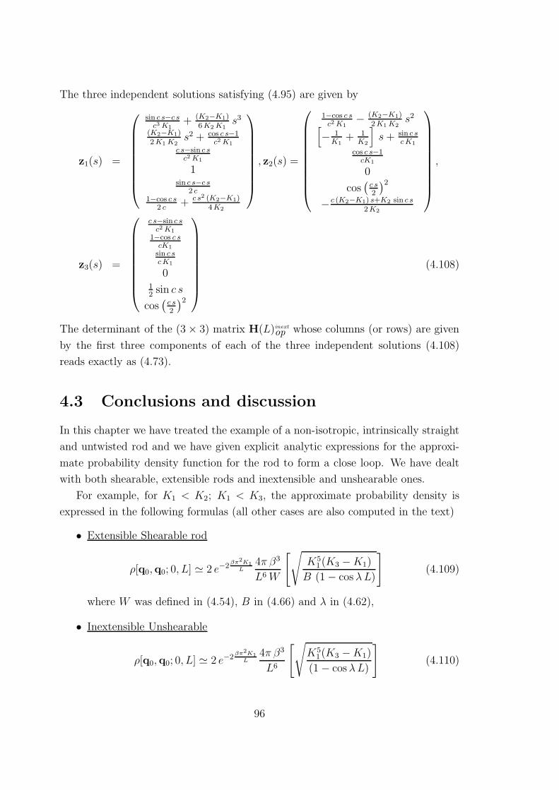
The three independent solutions satisfying (4.95) are given by
z1(s) =
sin c s−c sc3 K1
+ (K2−K1)6 K2 K1
s3
(K2−K1)2 K1 K2
s2 + cos c s−1c2 K1
c s−sin c sc2 K1
1sin c s−c s
2 c1−cos c s
2 c+ c s2 (K2−K1)
4 K2
, z2(s) =
1−cos c sc2 K1
− (K2−K1)2 K1 K2
s2
[
− 1K1
+ 1K2
]
s + sin c sc K1
cos c s−1cK1
0
cos(
c s2
)2
− c (K2−K1) s+K2 sin c s2 K2
,
z3(s) =
c s−sin c sc2 K1
1−cos c scK1
sin c sc K1
012sin c s
cos(
c s2
)2
(4.108)
The determinant of the (3 × 3) matrix H(L)inext
op whose columns (or rows) are given
by the first three components of each of the three independent solutions (4.108)
reads exactly as (4.73).
4.3 Conclusions and discussion
In this chapter we have treated the example of a non-isotropic, intrinsically straight
and untwisted rod and we have given explicit analytic expressions for the approxi-
mate probability density function for the rod to form a close loop. We have dealt
with both shearable, extensible rods and inextensible and unshearable ones.
For example, for K1 < K2; K1 < K3, the approximate probability density is
expressed in the following formulas (all other cases are also computed in the text)
• Extensible Shearable rod
ρ[q0,q0; 0, L] ≃ 2 e−2βπ2K1
L4π β3
L6 W
[√
K51 (K3 − K1)
B (1 − cos λ L)
]
(4.109)
where W was defined in (4.54), B in (4.66) and λ in (4.62),
• Inextensible Unshearable
ρ[q0,q0; 0, L] ≃ 2 e−2βπ2K1
L4π β3
L6
[√
K51(K3 − K1)
(1 − cos λ L)
]
(4.110)
96
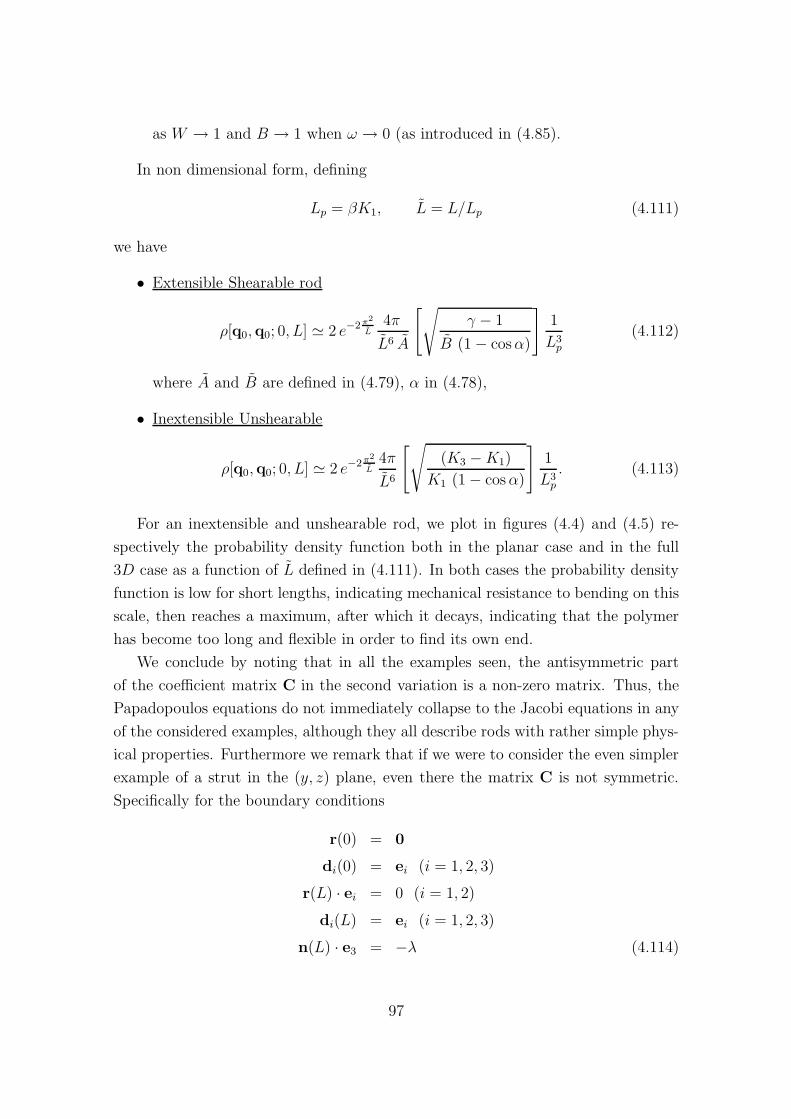
as W → 1 and B → 1 when ω → 0 (as introduced in (4.85).
In non dimensional form, defining
Lp = βK1, L = L/Lp (4.111)
we have
• Extensible Shearable rod
ρ[q0,q0; 0, L] ≃ 2 e−2π2
L4π
L6 A
[√
γ − 1
B (1 − cos α)
]
1
L3p
(4.112)
where A and B are defined in (4.79), α in (4.78),
• Inextensible Unshearable
ρ[q0,q0; 0, L] ≃ 2 e−2π2
L4π
L6
[√
(K3 − K1)
K1 (1 − cos α)
]
1
L3p
. (4.113)
For an inextensible and unshearable rod, we plot in figures (4.4) and (4.5) re-
spectively the probability density function both in the planar case and in the full
3D case as a function of L defined in (4.111). In both cases the probability density
function is low for short lengths, indicating mechanical resistance to bending on this
scale, then reaches a maximum, after which it decays, indicating that the polymer
has become too long and flexible in order to find its own end.
We conclude by noting that in all the examples seen, the antisymmetric part
of the coefficient matrix C in the second variation is a non-zero matrix. Thus, the
Papadopoulos equations do not immediately collapse to the Jacobi equations in any
of the considered examples, although they all describe rods with rather simple phys-
ical properties. Furthermore we remark that if we were to consider the even simpler
example of a strut in the (y, z) plane, even there the matrix C is not symmetric.
Specifically for the boundary conditions
r(0) = 0
di(0) = ei (i = 1, 2, 3)
r(L) · ei = 0 (i = 1, 2)
di(L) = ei (i = 1, 2, 3)
n(L) · e3 = −λ (4.114)
97
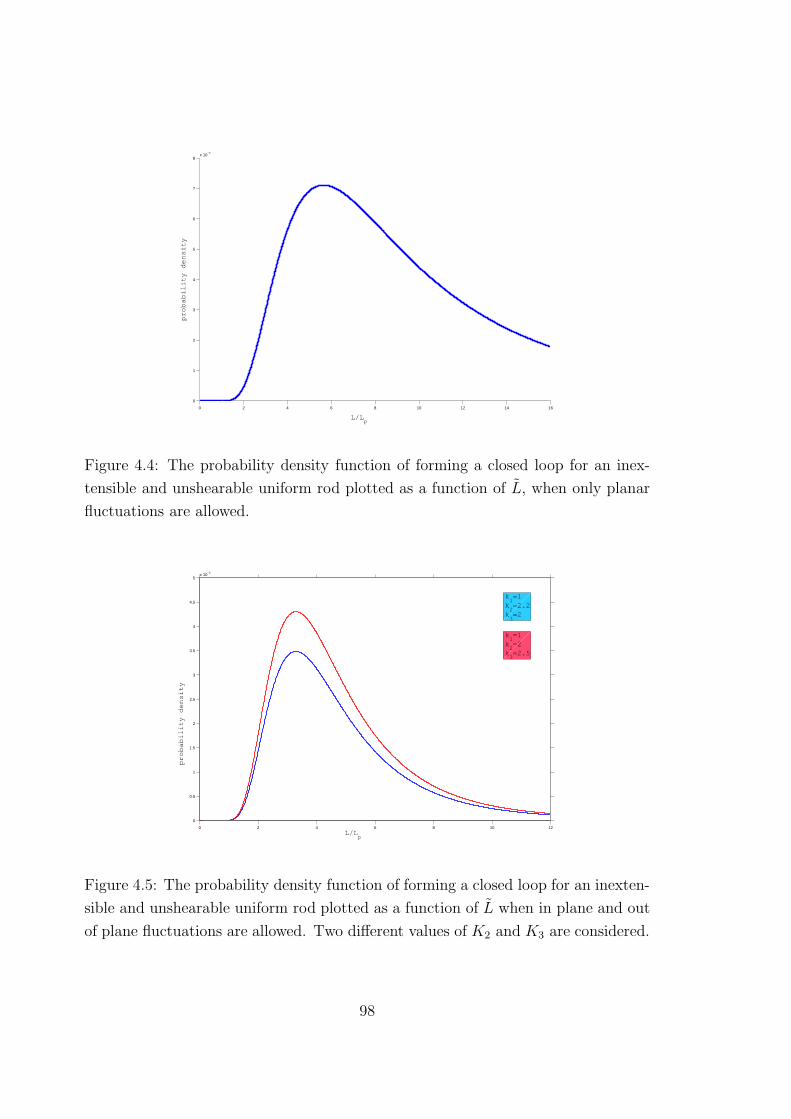
0 2 4 6 8 10 12 14 16
0
1
2
3
4
5
6
7
8x 10
−4
L/Lp
probability density
Figure 4.4: The probability density function of forming a closed loop for an inex-
tensible and unshearable uniform rod plotted as a function of L, when only planar
fluctuations are allowed.
0 2 4 6 8 10 12
0
0.5
1
1.5
2
2.5
3
3.5
4
4.5
5x 10
−5
L/Lp
probability density
k1=1
k2=2.2
k3=2
k1=1
k2=2
k3=2.5
Figure 4.5: The probability density function of forming a closed loop for an inexten-
sible and unshearable uniform rod plotted as a function of L when in plane and out
of plane fluctuations are allowed. Two different values of K2 and K3 are considered.
98
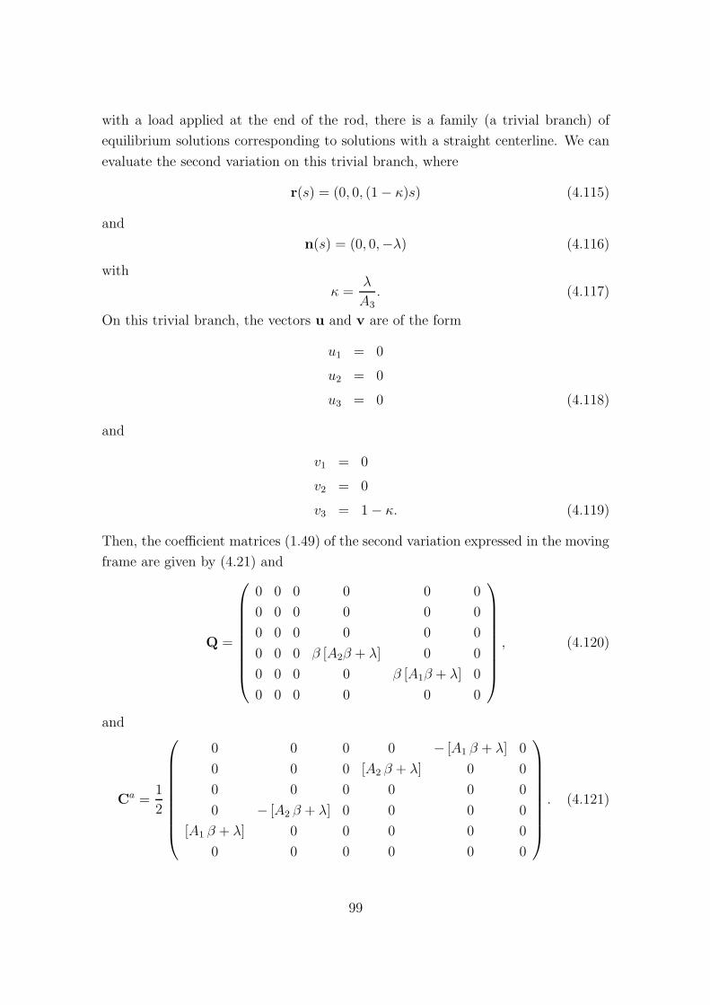
with a load applied at the end of the rod, there is a family (a trivial branch) of
equilibrium solutions corresponding to solutions with a straight centerline. We can
evaluate the second variation on this trivial branch, where
r(s) = (0, 0, (1 − κ)s) (4.115)
and
n(s) = (0, 0,−λ) (4.116)
with
κ =λ
A3. (4.117)
On this trivial branch, the vectors u and v are of the form
u1 = 0
u2 = 0
u3 = 0 (4.118)
and
v1 = 0
v2 = 0
v3 = 1 − κ. (4.119)
Then, the coefficient matrices (1.49) of the second variation expressed in the moving
frame are given by (4.21) and
Q =
0 0 0 0 0 0
0 0 0 0 0 0
0 0 0 0 0 0
0 0 0 β [A2β + λ] 0 0
0 0 0 0 β [A1β + λ] 0
0 0 0 0 0 0
, (4.120)
and
Ca =1
2
0 0 0 0 − [A1 β + λ] 0
0 0 0 [A2 β + λ] 0 0
0 0 0 0 0 0
0 − [A2 β + λ] 0 0 0 0
[A1 β + λ] 0 0 0 0 0
0 0 0 0 0 0
. (4.121)
99

From (4.121) it is then clear that even in this extremely simple example the approach
we have derived in Chapter 2 and 3 is unavoidable.
100
Conclusions
In this thesis we have demonstrated that a functional integral formulation allows
an approximate evaluation of DNA looping probabilities when the DNA is modeled
as a continuum elastic rod in thermodynamic equilibrium with a solvent (or heat
bath). In particular we have shown that if the energy scale β is large with respect to
the mechanical energy stored within the chain, and if the minimal energy configura-
tion between specified end conditions is locally unique, then the probability density
function for the chain to have its end-point at a fixed configuration q(L) = qL
in configuration space, including up to quadratic fluctuations about the associated
minimal energy configuration q, can be expressed as
ρ[q0,qL; 0, L] ≃ e−βE|q
√
det
(
β
2πV−1(L)
)
where each column of VT satisfies the linear system of Jacobi equations for the
second variation of the functional energy E associated to the configuration.
The first part of the proof is a translation to the case of real-valued path-integrals
of results of Papadopoulos [43] derived for the imaginary path-integrals arising in
quantum mechanical system. The second part of the proof is the introduction of the
non-linear change of variables
V−1dV
dsP = D−1dD
dsP + Ca
associating solutions D of the non-linear Papadopoulos matrix equation to the ma-
trix of Jacobi fields VT satisfying the linear Jacobi equations and appropriate initial
conditions. These two matrices trivially coincide (and the nonlinear terms in the
Papadopoulos equations vanish) in the absence of cross terms (Ca = 0) in the sec-
ond variation of the functional energy. However, in the presence of cross-terms, as
is typical for elastic rods modeling DNA, the change of variables is both necessary
and nontrivial. The third part of the proof is the observation that the two matrix
solutions D(s) and VT (s) share the same determinant, which is the only ingredient
appearing in our formula for the approximation of the probability density function.
Thus the path-integral formulation of the approximate, or semi-classical, probability
density function including quadratic fluctuations can be evaluated in terms of the
assumed local energy minimizer satisfying the prescribed end-point conditions and
the solution of an initial value problem for the associated linear Jacobi differential
equations.
Furthermore, we have shown that for shearable, extensible elastic rods that are
described in configuration space as framed curves, and therefore by pairs of inde-
pendent variables q(s) = (r(s),R(s)), with r(s) ∈ R3 and R(s) ∈ SO(3), the
probability density can be expressed as in the formula above, where the measure
in configuration space is provided by means of an appropriate parametrization of
the Euler parameters or quaternions. Within the context of elastic rods we have
thus provided a method to evaluate, up to second order corrections, the probability
density function of finding one end of the rod at a fixed location and orientation
as a function of the associated minimum energy configuration and the Jacobi fields
associated with the second variation.
In rod theory, and in particular in models of DNA, it is common to assume a con-
strained theory in which the variable r(s) is slaved to R(s) through the constraints
of inextensibility and unshearability, with the only vestige of the centerline r(s) be-
ing three scalar, isoperimetric constraints on R(s) expressing boundary conditions
on r. We also showed that our semi-classical path integral formulation extends
to this constrained problem merely by dint of taking the appropriate inextensible,
unshearable limit in the Hamiltonian form of the associated Jacobi equations.
For someone familiar with the path-integral literature, the fact that the semi-
classical approximation involves a determinant of a set of solutions to the Jacobi
equations is unsurprising [48] [52] [54] [57] . Nevertheless we believe the proof of this
fact for real-valued path integrals, and in the presence of cross terms in the second
variation to be original. As regards the application, the problem of DNA looping
including models involving rods is currently a rather active research domain, but
there is nothing in the literature that refers to the Jacobi field as a means to evaluate
probability density functions. This may in part be due to the fact that it is typical to
adopt an inextensible, unshearable model of DNA for which the appropriate system
of Jacobi equations are not widely known–the only modern citation of which we are
aware is [33]. We were only able to realize the appropriate semi-classical result for
this constrained model from the limit (in the Hamiltonian version) of the appropriate
102
Jacobi system in the unconstrained model.
In the last chapter of the thesis, we provide completely explicit, analytic expres-
sions for the semi-classical probability density function for the particular case of
a uniform, non-isotropic, intrinsically straight and untwisted rod to form a closed
loop.
The main theoretical concerns which are not discussed in this thesis are related
to the existence of
• multiple, but isolated minima,
• conjugate points,
• non-isolated minima.
Throughout the derivation we have assumed the existence of a unique minimizer
of the energy E for the given boundary data. However it is known that the boundary
value problems for elastic rods modeling DNA frequently do exhibit multiple minima.
Around each isolated minimizer the analysis presented here could still be applied,
and consequently, a second order correction as expressed in the formulas above may
be computed. The total probability density of forming a loop with boundary condi-
tions which admit distinct isolated minimizers, will thus be given by the sum of each
individual probability density as computed around the respective minimizers. For
instance, in the example of Chapter 4, closed loops could be formed with both left
and right handed circles (because the director framing allows a distinction between
these two cases), and in our theoretical derivation the two circles are considered as
distinct minimizers, so that (in this case by symmetry) the total probability density
of any circular loop forming would be twice that predicted by the semi-classical
computation at one of the circles. Similarly, in principle, the total looping proba-
bility of any closed configuration would have contributions from double and triple
covered circles, and single and multiple covered figure eight configurations, although
the comparatively high energy of these equilibria and the associated small value of
the pre-factor in the semi-classical probability density function would presumably
mean that their contribution is negligible.
The absence of conjugate points, that is points 0 < s < L where a non trivial
solution to the Jacobi equations vanishes, is a completely natural restriction in the
theory described here. As a conjugate point is approached the semi-classical prob-
ability density will diverge. In fact at that specific s, the matrix of Jacobi fields
will have linearly dependent columns, and the matrix itself will be singular with
103
vanishing determinant. If the conjugate point occurs within the interval considered,
the whole algebraic argument used to derive the Papadopoulos equations [43] fails,
as well as the non-linear change of variables, which relies on the non-singularity of
the matrices D(s) and V(s), ∀s 6= 0. That this is the case is completely natural,
as absence of a conjugate point is intrinsically associated with the stability proper-
ties of equilibrium configurations. For unconstrained problems it is well-known that
when Legendre’s strengthened condition is satisfied, in our case whenever the sym-
metric stiffness matrix is positive definite, then the absence of any conjugate point
is a necessary condition for a given equilibrium configuration to actually be a local
minimizer for the energy. Analogous results have been proven for isoperimetrically
constrained systems, including the case of inextensible, unshearable rods that is of
interest here [33], [40]. In other words, the theory should break down as soon as
a conjugate point is reached, as the configuration around which perturbations are
being considered ceases to be a local minimizer for the associated energy.
We remark that in the quantum mechanics literature for the case of imaginary
path-integrals, the presence of conjugate points is a much more delicate issue. In
the context of semi-classical quantum mechanics, the singularities of the Van-Hove-
Morette determinant have been discussed for the first time by P. Choquard [57]. In
this context there are results such as the Gutzwiller formula [65], which provides a
correction to the semi-classical kernel through a phase factor related to the Maslov-
Morse index, which in turn quantifies the dimension of the space over which the
second variation is negative.
In the case of real path-integrals and the application of looping of DNA, one
context where the presence of conjugate points is to be expected and should be
treated is that of isotropic boundary value problems, where the equilibria are local
minima, but are non-isolated because of a continuous symmetry that generates a
family of local minima. Perhaps the simplest case of this is the three-dimensional
looping problem described in Chapter 4 for an isotropic rod, for example the case
K1 = K2 and A1 = A2. Then there are not only right and left circular equilibria, but
a one-parameter family of circular loops with left and right pairs lying in each dif-
ferent plane containing the prescribed tangent. In that example s = L is necessarily
a conjugate point because of the non-isolation, so that the semi-classical formula as
stated does not apply. To handle this problem in future work it should be possible to
restrict fluctuations to those orthogonal to the null eigenfunction corresponding to
the conjugate point to obtain a finite semi-classical correction, and then to integrate
around the orbit of all equilibria to obtain an overall probability density function.
104
As far as biologically relevant applications of the theory developed here are con-
cerned, further research should go in at least three distinct directions, namely
• understanding regimes in which the semi-classical approximation is valid,
• implementing sequence dependence,
• extending the theory to more general looping problems.
Each of these directions appears to require the addition of numerical computation.
It has thus far not been stressed, but one of the major benefits of the semi-classical
formulas developed here is that they are highly amenable to numerics. The numerical
computation of the energy minimizer involves the solution of the Euler-Lagrange
equations, i.e. a nonlinear two-point boundary value problem. This is a nontrivial
numerical task, but various methods involving symmetry breaking and parameter
continuation have now been sufficiently developed [19] [32] [34] that it can now
be regarded as routine in the context of DNA looping equilibria. In any case,
computation of the equilibrium shape is an unavoidable part of any simulation.
An attractive feature of the fluctuation correction term is that it involves only the
numerical solution of a matrix, linear, ordinary differential equation with appropriate
initial value conditions.
We are unaware of any analytic result, or error estimate, quantifying the level of
approximation involved in considering only quadratic fluctuations. In the context of
DNA, the expectation is that for sufficiently short segments the elastic energy in the
pre-factor will dominate the fluctuation correction. The simple examples considered
in Chapter 4 would be useful to further analyze and quantify this expectation. In
these examples the semi-classical probability density function is known explicitly
as a function of all the parameters in the problem, so that numerical implementa-
tions of code to evaluate the formula can be found. More interestingly the problems
are simple enough that direct comparison with a relatively small number of com-
putationally intensive Monte Carlo simulations could be carried out for ranges of
parameter values to gain insight into the accuracy of the semi-classical formulas.
To include sequence dependence in a computational evaluation of the semi-
classical formula is relatively straightforward. The only critical point is that ac-
curate sequence-dependent parameter sets for DNA are not known, or at least are
not generally accepted. In particular, although the theory that has been derived is
for energy densities at most quadratic in their variables, this quadratic energy could
be regarded as the first terms in a Taylor expansion of any given energy functional.
105
Until at least these quadratic coefficients are known for DNA to a reasonable level
of accuracy an extension of our theory to non-quadratic energy densities does not
appear to be a pressing issue.
A more interesting generalization lies in other conditional probability densities
that could reasonably be interpreted as looping in a biological context. Specifically
one could study the probability that the two ends r(0) and r(L) coincide with no
requirement on the orientations R(0) and R(L). An analysis of this problem would
require a relaxation of the assumption of Dirichlet boundary conditions on location
and orientation at both ends. Such a generalization seems to be analytically quite
feasible.
To conclude, the semi-classical probability density function formulas that we
have obtained are of quite general applicability, especially as, in contrast to prior
theories for predicting looping, no assumption is made on uniformity of the chain,
or on isotropy, or on the presence or absence of the integral constraints that arise in
inextensible, unshearable models for DNA. Thus, we believe that the theory derived
here to be rather robust and to have the potential to describe a variety of different
situations which are of relevance to understanding DNA looping in vivo and in
analyzing ongoing experiments aimed at understanding sequence-dependent effects
in the mechanical properties of DNA.
106
Bibliography
[1] J. Watson and F. Crick, “Molecular structure of nucleic acids: a structure for
deoxyribose nucleic acid”, Nature 171 (4356), 737-738 (1953).
[2] D. A. Perlman et al. “AMBER, a package of computer programs for ap-
plying molecular mechanics, normal mode analysis, molecular dynamics and
free energy calculations to simulate the structural and energetic properties of
molecules”, Comp. Phys. Commun, 91, 1-41.
[3] W. Humphrey, A. Dalke and K. Schulten, “VMD-Visual Molecular Dynamics”,
Journal of Molecular Graphics, 14, 33-38 (1996).
[4] R. Schleif, “DNA looping”, Science 240 (4849), 127-128 (1988). R. Schleif,
“DNA looping”, Ann. Rev. Biochem. 61, 199-223 (1992).
[5] K. S. Matthews, “DNA looping”, Microbiol. Rev. 56, 123-136 (1992).
[6] L. Saiz and J. M. G. Vilar, “DNA looping: the consequences and its control”,
Curr. Opin. Struct. Biol, 16, 344-350 (2006).
[7] J. M. G. Vilar and S. Leibler, “DNA looping and physical constraints on tran-
scription regulation”, J. Mol. Biol. 331, 981-989 (2003).
[8] S. Jun and J. Bechhoefer, “Role of polymer loops in DNA replication”, Physics
in Canada 59(2), 85-92 (2003).
[9] R. Metzler et al., “Single DNA conformations and biological function”, J. Comp.
Theor. Nanoscience 4 (1), 1-49 (2007).
[10] H. Garcia et al., “Biological consequences of tightly bent DNA: the other life
of a macromolecular celebrity”, Biopolymers 85 (2), 115-130 (2006).
107
[11] D. Shore, J. Langowski and R. L. Baldwin, “DNA flexibility studied by covalent
closure of short fragments into circles”, Proc. Natl. Acad. Sci. 78, 4833-4837
(1981). D. Shore and R. L. Baldwin, “Energetics of DNA twisting. I. Relation
between twist and cyclization probability”, J. Mol. Biol. 170, 957-981 (1983).
[12] J. D. Kahn and D. M. Crothers, “Protein-induced bending and DNA cycliza-
tion”, Proc. Natl. Acad. Sci. 89, 6343-6347 (1992).
[13] Y. Zhang, D. M. Crothers, “Statistical mechanics of sequence-dependent cir-
cular DNA and its application for DNA cyclization”, Biophys. J. 84, 136-153
(2003).
[14] T. E. Cloutier and J. Widom, “Spontaneous sharp bending of double stranded
DNA”, Molecular Cell 14, 355-362 (2004).
[15] Q. Du et al., “Cyclization of short DNA fragments and bending fluctuations of
the double helix”, Proc. Natl. Acad. Sci. 102, 5397-5402(2005).
[16] J. Shimada, H. Yamakawa, “Ring-closure probabilities for twisted wormlike
chains”, Macromolecules 17, 689-698 (1984).
[17] H. Yamakawa and W. H. Stockmayer, “Statistical mechanics of wormlike chains.
II. Excluded volume effects”, J. Chem. Phys. 57, 2843-2854 (1972).
[18] H. Jacobson and W. H. Stockmayer, “Intramolecular reaction in polycondensa-
tions. I. The theory of linear systems”, J. Chem. Phys. 18, 1600-1606 (1950).
[19] R. S. Manning, J. H. Maddocks and J. D. Kahn, “A continuum rod model
of sequence-dependent DNA structure”, J. Chem. Phys. 105 (13), 5626-5646
(1996).
[20] J. Yan and J. F. Marko, “Localized single-stranded bubble mechanism for cy-
clization of short double helix DNA”, Phys. Rev. Lett. 93 108108-1/4 (2004).
[21] S. Rappaport and Y. Rabin, “Effect of spontaneous curvature and sequence
disorder on cyclization of fluctuating filaments”, Macromolecules 37 (21), 7847-
7849 (2004). S. Rappaport and Y. Rabin, “Effect of spontaneous curvature and
twist rigidity on cyclization of fluctuating filaments”, Biophys. J. 88 (1), 59A-
59A Suppl. S (2005).
108
[22] A. J. Spakowitz and Z. G. Wang,“Exact results for a semiflexible polymer chain
in an aligning field”, Macromolecules 37, 5814-5823 (2004). A. J. Spakowitz and
Z. G. Wang,“End-to-end distance vector distribution with fixed end orientations
for the wormlike chain model”, Phys. Rev. E 72, 041802-1-13 (2005)
[23] P. A. Wiggins, R. Phillips and P. C. Nelson, “Exact theory of kinkable elastic
polymers”, Phys. Rev. 71 021909 (2005).
[24] E. Villa, A. Balaeff and K. Schulten, “Structural dynamics of the Lac-repressor
DNA complex revealed by a multiscale simulation”, Proc. Natl. Acad. Sci. 102,
6783-6788 (2005).
[25] L. Czapla, D. Swigon and W. K. Olson, “Sequence-dependent effects in the
cyclization of short DNA”, J. Chem. Theory Comput. 2, 685-695 (2006).
[26] D. Swigon, B. D. Coleman and W. K. Olson, “Modeling the Lac-repressor oper-
ator assembly. I, The influence of DNA looping on Lac-repressor conformation”,
Proc. Natl. Acad. Sci. 103, 9879-9884 (2006).
[27] P. K. Purohit and P. C. Nelson, “Effect of supercoiling on formation of protein-
mediated DNA loops”, Phys. Rev. E 74, 061907-1-14 (2006).
[28] P. A. Wiggins and P. C. Nelson, “A generalized theory of semiflexible polymers”,
Phys. Rev. E, 73, 0319061-1-13 (2006).
[29] F. Lankas, R. Lavery and J. H. Maddocks, “Kinking occurs during molecular
dynamics simulations of small DNA minicircles”, Structure 14 (10) 1527-1534
(2006).
[30] C. J. Benham, “An elastic model of the large-scale structure of duplex DNA”,
Biopolymers 18, 609-623 (1979). C. J. Benham, “Elastic model of supercoiling”,
Proc. Natl. Acad. Sci. 77, 2397-2401 (1977).
[31] B. D. Coleman, W. K. Olson and D. Swigon, “Theory of sequence-dependent
DNA elasticity”, J. Chem. Phys. 188, 7127-7140 (2003).
[32] R. S. Manning and J. H. Maddocks, “Symmetry breaking and the twisted elastic
ring”, Comput. Methods. Appl. Mech. Engrg. 170, 313-330 (1999).
[33] R. S. Manning, K. A. Rogers and J. H. Maddocks, “Isoperimetric conjugate
points with application to the stability of DNA minicircles”, Proc. R. Soc.
Lond. A 454, 3047-3074 (1998).
109
[34] P. B. Furrer, R. S. Manning and J. H. Maddocks, “DNA rings with multiple
energy minima”, Biophysical Journal 79 (1), 116-136 (2000).
[35] E. and F. Cosserat, “Theorie des Corps Deformables”, Hermann, Paris (1909).
[36] N. Chouaieb, “Kirchhoff’s problem of helical solutions of uniform rods and their
stability properties”, These 2717, Ecole Polytecnique Federale de Lausanne
(2003).
[37] S. S. Antman, Nonlinear Problems of Elasticity, Springer-Verlag, New-York
(1995).
[38] D. J. Dichmann, Y. Li and J. H. Maddocks, “Hamiltonian Formulations and
Symmetries in Rod Mechanics”, IMA Volumes in Mathematics and its Appli-
cations, ed. J. P. Mesirov, K. Schulten, D. Sumners 82 (1996) Springer Verlag,
71-113.
[39] Y. Li and J. H. Maddocks, “On the computation of equilibria of elastic
rods. Part I: integrals, symmetry and a hamiltonian formulation”, unpublished
(1996).
[40] K. A. Rogers, “Stability exchange in parameter-dependent constrained varia-
tional principles with applications to elastic rod models of DNA minicircles”,
PhD dissertation, University of Maryland, College Park (1997).
[41] N. Chouaieb and J. H. Maddocks, “Kirchhoff’s problem of helical equilibria of
uniform rods”, J. Elasticity 77, 221-247 (2004).
[42] I. M. Gelfand and S. V. Fomin, “Calculus of variations”, ed. Prentice-Hall,
1963.
[43] G. J. Papadopoulos, “Gaussian path integrals”, Phys. Rev. D 11, 2870-2875
(1975).
[44] W. T. Reid, Riccati Differential equations, Academic Press, New York and
London (1972).
[45] R. W. R. Darling, “Converting Matrix Riccati Equations to second-order linear
ODE”, SIAM Rev. Vol. 39 No. 3, 508-510 (1997).
[46] R. P. Feynman and A. R. Hibbs, “Quantum mechanics and path integrals”, ed.
McGraw-Hill, 1965.
110
[47] M. Chaichian and A. Demichev, Path Integrals in Physics. Volume I: Stochastic
Processes and Quantum Mechanics, Institute of Physics Publishing, 2001.
[48] L. S. Schulman, “Techniques and applications of path integration”, ed. John
Wiley & Sons, 1981.
[49] F. W. Wiegel, Introduction to Path Integral Methods in Physics and Polymer
Science, World Scientific Publishing, 1986.
[50] C. Morette, “On the definition and approximation of Feynman’s path integrals”,
Phys. Rev. 81, 848-852 (1951).
[51] C. DeWitt-Morette, “Feynman’s path integral. Definition without limiting pro-
cedure”, Commun. Math. Phys. 28, 47-67 (1972).
[52] C. DeWitt-Morette, “The semiclassical expansion”, Ann. Phys. 97, 367-399
(1976).
[53] G. Freiling, “A survey of nonsymmetric Riccati equations”, Linear Algebra and
its Applications, 351-352 (2002) 243-270.
[54] Ph. Choquard and F. Steiner, The story of Van Vleck’s and Morette-Van Hove’s
determinants, Helv. Phys. Acta 69, 636-652, 1996.
[55] G. J. Papadopoulos, private comunication.
[56] I. M. Gelfand and A. M. Yaglom, “Integration in functional spaces and its
applications in quantum physics”, J. Math. Phys. 1, 48-69 (1960).
[57] C. Grosche and F. Steiner, “Handbook of Feynman path integrals”, ed.
Springer, 1998.
[58] L. Nachbin, The Haar integral, D. Van Nostrand Company, 1965.
[59] D. H. Sattinger and O. L. Weaver, Lie Groups and Algebras with Applications
to Physics, Geometry and Mechanics, Springer-Verlag New York Inc, 1986.
[60] Wu-Ki Tung, Group Theory in Physics, World Scientific Publishing, (1985).
[61] S. Stepanow, “Statistical mechanics of semiflexible polymers”, Eur. Phys. J. B.
39, 499-512 (2004).
111
[62] A. J. Spakowitz, “Wormlike chain statistics with twist and fixed ends”, Euro-
phys. Lett. 73 (5), 684-690 (2006).
[63] Y. Zhang et al., “Statistical mechanical theory of DNA looping”, Biolphysical
Journal 90, 1903-1912 (2006).
[64] C. Vaillant et al, “Formation and positioning of nucleosomes: effect of sequence-
dependent long-range correlated structural disorder”, Eur. Phys. J. E. 19, 263-
277 (2006).
[65] M. C. Gutzwiller, Chaos in Classical and Quantum Mechanics, Springer-Verlag,
1980.
112

Curriculum Vitae
I was born in that lovely polluted city of Milano, Italy. I was raised happily among an
extended family of scientists and music lovers. As far as my education is concerned
• 2003-
PhD student and assistante doctorante under the supervision of Prof. John
H. Maddocks, Chaire d’Analyse Appliquee, Ecole Polytecnique de Lausanne,
Switzerand.
• 2004
MPhil, Insitute of Cosmology and Gravitation, Portsmouth University. Dis-
sertation title: Low-energy effective theory for brane-world models. Advisor:
Prof. David Wands, Insitute of Cosmology and Gravitation, Portsmouth Uni-
versity.
• 2002
Degree in Physics with honors (110/110 cum laude), Universita degli Studi
di Milano, Italy. Dissertation title: Cosmological implications of scenarios
with infinite extra-dimensions. Advisors: Prof. Daniela Zanon, Universita
degli Studi di Milano, Italy; Prof. Sabino Matarrese, Universita degli Studi
di Padova, Italy and Prof. Antonio Riotto, Universita degli Studi di Padova,
Italy.
Pubblications:
• Ludovica Cotta-Ramusino and David Wands, Low-energy effective theory for a
Randall-Sundrum scenario with a moving bulk brane, Phys. Rev. D, 75 104001-
1-9 (2007).
Awards:
• 2006
Teaching Award: Prime de rendiment , EPFL Lausanne, CH.
113
• 2002
Research Award: Introduction to Research in Mathematics, Department of
Mathematics Universita degli Studi di Milano, IT.
114

![1 –cosa: worldview(s) · (Parmenide, Poema sulla Natura, frammento 2) SeedQuestions (b) ... Subjectarea of design: pattern [schemi di relazioni] Relazionismo SeedQuestions](https://img.pdfslide.us/doc/110x75/5c6925e109d3f242168c91fa/1-cosa-worldviews-parmenide-poema-sulla-natura-frammento-2-seedquestions.jpg)


![Home []all. 10...2009/04/16 · e-mail: Fraqcesco.pinto-1949@poste.it On.le CONSIGLIO DELL'ORDINE AVVOCATI Palazzo di Giustizia CATANZARO Oggetto: Prot. n. 1904/2009 — Istanza di](https://img.pdfslide.us/doc/110x75/60916e1a6c97c15814777ada/home-all-10-20090416-e-mail-fraqcescopinto-1949posteit-onle-consiglio.jpg)