Embed Size (px)
Citation preview

Lower bounds for small depth arithmetic circuits
Chandan Saha
Joint work with Neeraj Kayal (MSRI) Nutan Limaye (IITB)
Srikanth Srinivasan (IITB)

Arithmetic Circuit: A model of computation
+
x x x x
+ + + +
x x x x
….
…..
x1 x2 xn-1 xn
f(x1, x2, …, xn) --> multivariate polynomial in x1, …, xn
x
g h
gh
+
g h
g+h
Product gate
Sum gate
There are `field constants’ on the wires

Arithmetic Circuit: A model of computation
+
x x x x
+ + + +
x x x x
….
…..
x1 x2 xn-1 xn
f(x1, x2, …, xn)
Depth = 4

Arithmetic Circuit: A model of computation
+
x x x x
+ + + +
x x x x
….
…..
x1 x2 xn-1 xn
f(x1, x2, …, xn)
Size = no. of gates and wires

The lower bound question
Is there an explicit family of n-variate, poly(n) degree polynomials fn that requires…
…super-polynomial in n circuit size ?

The lower bound question
Is there an explicit family of n-variate, poly(n) degree polynomials fn that requires…
…super-polynomial in n circuit size ?
Note : A random polynomial has super-poly(n) circuit size

The Permanent – an explicit family
Permn = ∑ ∏ xi σ(i)σ є Sn i є [n]

The Permanent – an explicit family
• Degree of Permn is low. i.e. bounded by poly(n)
Permn = ∑ ∏ xi σ(i)σ є Sn i є [n]

The Permanent – an explicit family
• Degree of Permn is low.
• Coefficient of any given monomial can be found efficiently. …given a monomial, there’s a poly-time algorithm to determine the coefficient of the monomial.
Permn = ∑ ∏ xi σ(i)σ є Sn i є [n]

The Permanent – an explicit family
• Degree of Permn is low.
• Coefficient of any given monomial can be found efficiently.
These two properties characterize explicitness
Permn = ∑ ∏ xi σ(i)σ є Sn i є [n]

The Permanent – an explicit family
• Degree of Permn is low.
• Coefficient of any given monomial can be found efficiently.
Define class VNP
Permn = ∑ ∏ xi σ(i)σ є Sn i є [n]

The Permanent – an explicit family
• Degree of Permn is low.
• Coefficient of any given monomial can be found efficiently.
Define class VNP
Permn = ∑ ∏ xi σ(i)σ є Sn i є [n]
Class VP: Contains families of low degree polynomials fn that can be computed by poly(n)-size circuits.

The Permanent – an explicit family
• Degree of Permn is low.
• Coefficient of any given monomial can be found efficiently.
Permn = ∑ ∏ xi σ(i)σ є Sn i є [n]
VP vs VNP: Does Permn family require super-poly(n) size circuits?

A strategy for proving arithmetic circuit lower bound
Step 1: Depth reduction
Step 2: Lower bound for small depth circuits

A strategy for proving arithmetic circuit lower bound
Step 1: Depth reduction
Step 2: Lower bound for small depth circuits

Notations and Terminologies
Notations: n = no. of variables in fn
d = degree bound on fn = nO(1)
Homogeneous polynomial: A polynomial is homogeneous if all its monomials have the same degree (say, d).
Homogeneous circuits: A circuit is homogeneous if every gate outputs/computes a homogeneous polynomial.
Multilinear polynomial: In every monomial, degree of every variable is at most 1.

Reduction to depth ≈ log d
Valiant, Skyum, Berkowitz, Rackoff (1983). Homogeneous, degree d, fn computed by poly(n) circuit
fn computed by homogeneous poly(n) circuit of depth O(log d)
arbitrary depth≈ log d
poly(n) poly(n)

Reduction to depth 4
Agrawal, Vinay (2008); Koiran (2010); Tavenas (2013).
Homogeneous, degree d, fn computed by poly(n) circuit
fn computed by homogeneous depth 4 circuit of size nO(√d)
≈ log d4
nO(√d) poly(n)

Reduction to depth 4
Agrawal, Vinay (2008); Koiran (2010); Tavenas (2013).
Homogeneous, degree d, fn computed by poly(n) circuit
fn computed by homogeneous depth 4 circuit of size nO(√d)
≈ log d4
nO(√d) poly(n)
… fn can have nO(d) monomials !

A depth 4 circuit
+
x x x x
+ + + +
x x x x
….
…..
x1 x2 xn-1 xn
∑
∏
∑
∏

A depth 4 circuit
+
x x x x
+ + + +
x x x x
….
…..
x1 x2 xn-1 xn
∑ ∏ Qiji j
sum of monomialsQij

Reduction to depth 3
Gupta, Kamath, Kayal, Saptharishi (2013); Tavenas (2013).
Homogeneous, degree d, fn computed by poly(n) circuit
fn computed by depth 3 circuit of size nO(√d)
3
nO(√d) nO(√d)
4

Reduction to depth 3
Gupta, Kamath, Kayal, Saptharishi (2013); Tavenas (2013).
Homogeneous, degree d, fn computed by poly(n) circuit
fn computed by depth 3 circuit of size nO(√d)
3
nO(√d) nO(√d)
4
not homogeneous!

A depth 3 circuit
+
x x x x
+ + + +….
x1 x2 xn-1 xn
∑ ∏ liji j
linear polynomiallij
bottom fanin

Implication of the depth reductions
Let fn be an explicit family of polynomials.
if fn takes nω(√d) size homogeneous
if fn takes nω(√d) size
VP ≠ VNP or
4
3
A strategy for proving arithmetic circuit lower bound
Step 1: Depth reduction
Step 2: Lower bound for small depth circuits

Lower bound for homogeneous depth 4
Theorem: There is a family of homogeneous polynomials fn in VNP (with deg fn = d) such that…
…any homogeneous depth-4 circuit computing fn has size nΩ(√d)
size = nΩ(√d)
4
fn

Lower bound for homogeneous depth 4
Theorem: There is a family of homogeneous polynomials fn in VNP (with deg fn = d) such that…
…any homogeneous depth-4 circuit computing fn has size nΩ(√d)
size = nΩ(√d)
4
fn
fn = i
∑ ∏ Qij
… has size nΩ(√d)
j
sum of monomials

Lower bound for homogeneous depth 4
Theorem: There is a family of homogeneous polynomials fn in VNP (with deg fn = d) such that…
…any homogeneous depth-4 circuit computing fn has size nΩ(√d)
size = nΩ(√d)
4
fn
…joint work with Kayal, Limaye , Srinivasan

Lower bound for homogeneous depth 4
Theorem: There is a family of homogeneous polynomials fn in VNP (with deg fn = d) such that…
…any homogeneous depth-4 circuit computing fn has size nΩ(√d)
size = nΩ(√d)
4
fn
…the technique appears to be using homogeneity crucially

Lower bound for depth 3
Theorem: There is a family of homogeneous polynomials fn in VNP (with deg fn = d) such that…
any depth-3 circuit (bottom fanin ≤ √d) computing fn has size nΩ(√d)
size = nΩ(√d)
3
fn

Lower bound for depth 3
Theorem: There is a family of homogeneous polynomials fn in VNP (with deg fn = d) such that…
any depth-3 circuit (bottom fanin ≤ √d) computing fn has size nΩ(√d)
size = nΩ(√d)
3
fn
needn’t be homogeneous

Lower bound for depth 3
Theorem: There is a family of homogeneous polynomials fn in VNP (with deg fn = d) such that…
any depth-3 circuit (bottom fanin ≤ √d) computing fn has size nΩ(√d)
size = nΩ(√d)
3
fn Note: Even for bottom fanin ≤ √d, depth-3 circuits nω(√d) VP ≠ VNP

Lower bound for depth 3
Theorem: There is a family of homogeneous polynomials fn in VNP (with deg fn = d) such that…
any depth-3 circuit (bottom fanin ≤ t) computing fn has size nΩ(d/t)
size = nΩ(d/t)
3
fn
…joint work with Kayal

Lower bound for depth 3
Theorem: There is a family of homogeneous polynomials fn in VNP (with deg fn = d) such that…
any depth-3 circuit (bottom fanin ≤ t) computing fn has size nΩ(d/t)
size = nΩ(d/t)
3
fn
… answers a question by Shpilka & Wigderson (1999)

Proof ideas

Homogeneous depth-4 lower bound

Complexity measure• A measure is a function μ: F[x1, …, xn] -> R.
• We wish to find a measure μ such that
1. If C is a circuit (say, a depth 4 circuit) then μ(C) ≤ s. “small quantity” , where s = size(C)
2. For an “explicit” polynomial fn , μ(fn) ≥ “large quantity”
• Implication: If C = fn then s ≥ “large quantity”
“small quantity”
Upper bound
Lower bound

Some complexity measures Measure Model
Partial derivatives (Nisan & Wigderson) homogeneous depth-3 circuits
Evaluation dimension (Raz) multilinear formulas
Hessian (Mignon & Ressayre) determinantal complexity permanent
Jacobian (Agrawal et. al.) occur-k, depth-4 circuits
Incomplete list ?

Some complexity measures Measure Model
Partial derivatives (Nisan & Wigderson) homogeneous depth-3 circuits
Evaluation dimension (Raz) multilinear formulas
Hessian (Mignon & Ressayre) determinantal complexity permanent
Jacobian (Agrawal et. al.) occur-k, depth-4 circuits
Shifted partials (Kayal; Gupta et. al.) homog. depth-4 with low bottom fanin
Projected shifted partials homogeneous depth-4 circuits;
depth-3 circuits (with low bottom fanin)

Space of Partial Derivatives Notations:
∂=k f : Set of all kth order derivatives of f(x1, …, xn)
< S > : The vector space spanned by F-linear combinations of polynomials in S
Definition: PDk(f) = dim(< ∂=k f >)
Sub-additive property: PDk(f1 + f2) ≤ PDk(f1) + PDk(f2)

Space of Shifted Partials
Notation: x=ℓ = Set of all monomials of degree ℓ
Definition: SPk,ℓ (f) := dim (< x=ℓ . ∂=k f >)
Sub-additivity: SPk,ℓ (f1 + f2) ≤ SPk,ℓ (f1) + SPk,ℓ (f2)

Space of Shifted Partials
Notation: x=ℓ = Set of all monomials of degree ℓ
Definition: SPk,ℓ (f) := dim (< x=ℓ . ∂=k f >)
Sub-additivity: SPk,ℓ (f1 + f2) ≤ SPk,ℓ (f1) + SPk,ℓ (f2)
Why do we expect SP(C) to be small ?

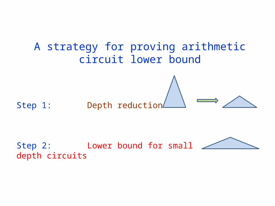
Shifted partials – the intuition C = Q11Q12…Q1m + … + Qs1Qs2…Qsm (homog. depth 4)
Qij = Sum of monomials

Shifted partials – the intuition C = Q11Q12…Q1m + … + Qs1Qs2…Qsm (homog. depth 4)
Observation: ∂=k Qi1…Qim has “many roots” if k << m << n
… any common root of Qi1…Qim is also a common root of ∂=k Qi1…Qim

Shifted partials – the intuition C = Q11Q12…Q1m + … + Qs1Qs2…Qsm (homog. depth 4)
Observation: Dimension of the variety of ∂=k Qi1…Qim is large if k << m << n
Shifted partials – the intuition C = Q11Q12…Q1m + … + Qs1Qs2…Qsm (homog. depth 4)
Observation: Dimension of the variety of ∂=k Qi1…Qim is large if k << m << n
[Hilbert’s] Theorem (informal): If dimension of the variety of g is large then dim (< x=ℓ . g >) is small.

Shifted partials – the intuition C = Q11Q12…Q1m + … + Qs1Qs2…Qsm (homog. depth 4)
Observation: Dimension of the variety of ∂=k Qi1…Qim is large if k << m << n
[Hilbert’s] Theorem (informal): If dimension of the variety of g is large then dim (< x=ℓ . g >) is small.
… so we expect SPk,ℓ (Qi1…Qim) to be a `small quantity’

Shifted partials – the intuition C = Q11Q12…Q1m + … + Qs1Qs2…Qsm (homog. depth 4)
Observation: Dimension of the variety of ∂=k Qi1…Qim is large if k << m << n
[Hilbert’s] Theorem (informal): If dimension of the variety of g is large then dim (< x=ℓ . g >) is small.
… by subadditivity, SPk,ℓ (C) ≤ s . `small quantity’

Depth-4 with low bottom degree C = Q11Q12…Q1m + … + Qs1Qs2…Qsm (homog. depth 4)
Qij = Sum of monomials of degree ≤ t(w.l.o.g m ≤ 2d/t )

Depth-4 with low bottom degree C = Q11Q12…Q1m + … + Qs1Qs2…Qsm
∂=k Qi1…Qim = Qi1 Qi2…Q ik …Qim + Qi1 Qi2…Q ik Q i k+1…Qim + … X
. . . . ..
= Qi k+1 … Qim + Qi1 Qi k+2 … Qim + …
degree ≤ k.t

Depth-4 with low bottom degree C = Q11Q12…Q1m + … + Qs1Qs2…Qsm
∂=k Qi1…Qim = Qi1 Qi2…Q ik …Qim + Qi1 Qi2…Q ik Q i k+1…Qim + … X
. . . . ..
= Qi k+1 … Qim + Qi1 Qi k+2 … Qim + …
at most ( ) termsmk

Depth-4 with low bottom degree C = Q11Q12…Q1m + … + Qs1Qs2…Qsm
∂=k Qi1…Qim = Qi1 Qi2…Q ik …Qim + Qi1 Qi2…Q ik Q i k+1…Qim + … X
. . . . ..
= Qi k+1 … Qim + Qi1 Qi k+2 … Qim + …
u . ∂=k Qi1…Qim = Qi k+1 … Qim + Qi1 Qi k+2 … Qim + …X
degree = ℓ degree ≤ ℓ + k.t

Depth-4 with low bottom degree C = Q11Q12…Q1m + … + Qs1Qs2…Qsm
∂=k Qi1…Qim = Qi1 Qi2…Q ik …Qim + Qi1 Qi2…Q ik Q i k+1…Qim + … X
. . . . ..
= Qi k+1 … Qim + Qi1 Qi k+2 … Qim + …
u . ∂=k Qi1…Qim = Qi k+1 … Qim + Qi1 Qi k+2 … Qim + …X
n + ℓ + ktn
mkSPk,ℓ
(Qi1…Qim) ≤ ( ) . ( )

Depth-4 with low bottom degree C = Q11Q12…Q1m + … + Qs1Qs2…Qsm
∂=k Qi1…Qim = Qi1 Qi2…Q ik …Qim + Qi1 Qi2…Q ik Q i k+1…Qim + … X
. . . . ..
= Qi k+1 … Qim + Qi1 Qi k+2 … Qim + …
u . ∂=k Qi1…Qim = Qi k+1 … Qim + Qi1 Qi k+2 … Qim + …X
n + ℓ + ktn
mkSPk,ℓ
(C) ≤ s. ( ) . ( ) Upper bound

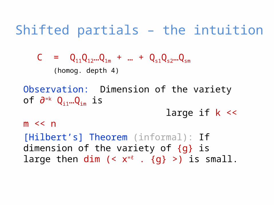
Reduction to low bottom degreeC = Q11Q12…Q1m + … + Qs1Qs2…Qsm (homog. depth 4)
Qij = Sum of monomials (NO degree restriction)

Reduction to low bottom degreeC = Q11Q12…Q1m + … + Qs1Qs2…Qsm
Idea: Reduce to the case of low bottom degree using
• Random restriction
• Multilinear projection

Reduction to low bottom degreeC = Q11Q12…Q1m + … + Qs1Qs2…Qsm
Random restriction: Set every variable to zero independently at random with a certain probability.
…denoted naturally by a map σ

Reduction to low bottom degreeC = Q11Q12…Q1m + … + Qs1Qs2…Qsm
Random restriction: Set every variable to zero independently at random with a certain probability.
…denoted naturally by a map σ
σ(C) = σ(Q11) σ(Q12)…σ(Q1m) + … + σ(Qs1) σ(Qs2)…σ(Qsm)
Obs: If a monomial u has many variables (high support) then σ(u) = 0 w.h.p

Reduction to low bottom degreeC = Q11Q12…Q1m + … + Qs1Qs2…Qsm
Random restriction: Set every variable to zero independently at random with a certain probability.
…denoted naturally by a map σ
σ(C) = σ(Q11) σ(Q12)…σ(Q1m) + … + σ(Qs1) σ(Qs2)…σ(Qsm)
w.l.o.g σ(Qij) = sum of ‘low support’ monomials

Reduction to low bottom degreeC = Q11Q12…Q1m + … + Qs1Qs2…Qsm
Random restriction: Set every variable to zero independently at random with a certain probability.
Homogeneous depth 4 homogenous depth 4 with low bottom support
… w.l.o.g assume that C has low bottom support
Reduction to low bottom degreeC = Q11Q12…Q1m + … + Qs1Qs2…Qsm
Projection map: π (g) = sum of the multilinear monomials in g

Reduction to low bottom degreeC = Q11Q12…Q1m + … + Qs1Qs2…Qsm
Projection map: π (g) = sum of the multilinear monomials in g
Observation: π (sum of ‘low support’ monomials) = sum of ‘low degree’ monomials

Reduction to low bottom degreeC = Q11Q12…Q1m + … + Qs1Qs2…Qsm
Projection map: π (g) = sum of the multilinear monomials in g
Observation:
π (Qij ) = sum of ‘low degree’ monomials

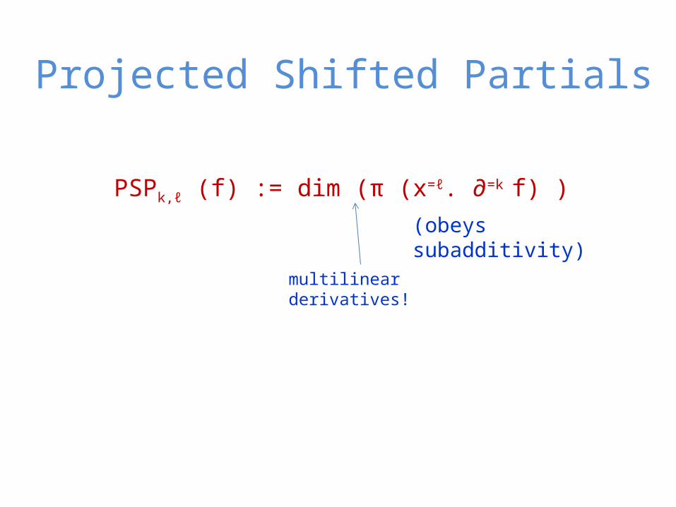
Projected Shifted Partials
PSPk,ℓ (f) := dim (π (x=ℓ. ∂=k f) )(obeys subadditivity)

Projected Shifted Partials
PSPk,ℓ (f) := dim (π (x=ℓ. ∂=k f) )(obeys subadditivity)
multilinear shifts only!
Projected Shifted Partials
PSPk,ℓ (f) := dim (π (x=ℓ. ∂=k f) )(obeys subadditivity)
multilinear derivatives!

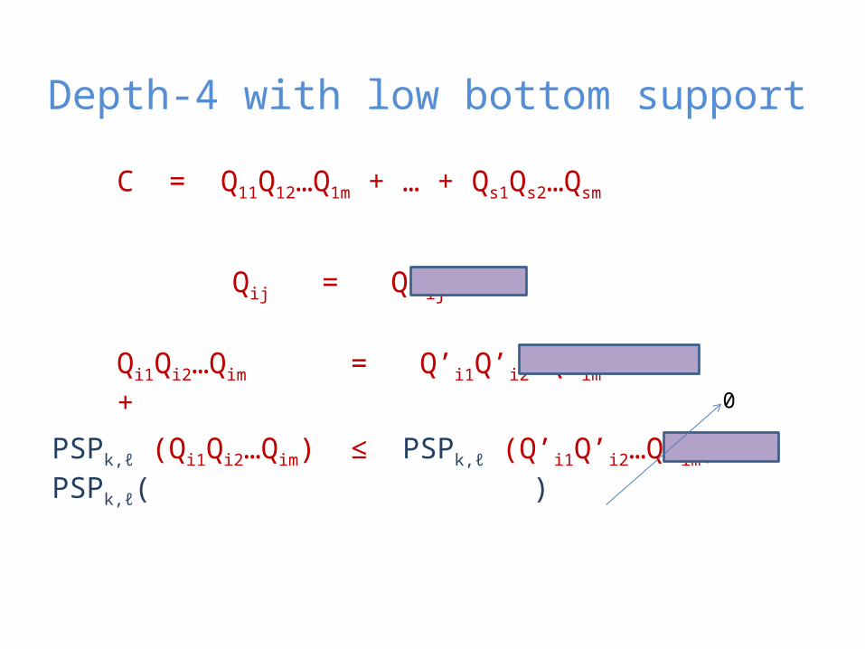
Depth-4 with low bottom support C = Q11Q12…Q1m + … + Qs1Qs2…Qsm
support of every monomial bounded by t

Depth-4 with low bottom support C = Q11Q12…Q1m + … + Qs1Qs2…Qsm
Qij = Q’ij +
Every variable in every monomial has degree 2 or less

Depth-4 with low bottom support C = Q11Q12…Q1m + … + Qs1Qs2…Qsm
Qij = Q’ij +
Every monomial has a variable with degree 3 or more

Depth-4 with low bottom support C = Q11Q12…Q1m + … + Qs1Qs2…Qsm
Qij = Q’ij +
Qi1Qi2…Qim = Q’i1Q’i2…Q’im +
Every monomial has a variable with degree 3 or more

Depth-4 with low bottom support C = Q11Q12…Q1m + … + Qs1Qs2…Qsm
Qij = Q’ij +
Qi1Qi2…Qim = Q’i1Q’i2…Q’im +
PSPk,ℓ (Qi1Qi2…Qim) ≤ PSPk,ℓ (Q’i1Q’i2…Q’im) + PSPk,ℓ( )
Depth-4 with low bottom support C = Q11Q12…Q1m + … + Qs1Qs2…Qsm
Qij = Q’ij +
Qi1Qi2…Qim = Q’i1Q’i2…Q’im +
PSPk,ℓ (Qi1Qi2…Qim) ≤ PSPk,ℓ (Q’i1Q’i2…Q’im) + PSPk,ℓ( )
0

Depth-4 with low bottom support C = Q11Q12…Q1m + … + Qs1Qs2…Qsm
Qij = Q’ij +
Qi1Qi2…Qim = Q’i1Q’i2…Q’im +
PSPk,ℓ (Qi1Qi2…Qim) ≤ PSPk,ℓ (Q’i1Q’i2…Q’im) + PSPk,ℓ( )
0
degree ≤ 2t

Depth-4 with low bottom support C = Q11Q12…Q1m + … + Qs1Qs2…Qsm
Qij = Q’ij +
Qi1Qi2…Qim = Q’i1Q’i2…Q’im +
PSPk,ℓ (Qi1Qi2…Qim) ≤ PSPk,ℓ (Q’i1Q’i2…Q’im)
Abusing notation: Call Q’ij as Qij

Depth-4 with low bottom support
∂=k Qi1…Qim = Qi1 Qi2…Q ik …Qim + Qi1 Qi2…Q ik Q i k+1…Qim + … X
. . . . ..
= Qi k+1 … Qim + Qi1 Qi k+2 … Qim + …
degree ≤ 2kt

Depth-4 with low bottom support
∂=k Qi1…Qim = Qi1 Qi2…Q ik …Qim + Qi1 Qi2…Q ik Q i k+1…Qim + … X
. . . . ..
= Qi k+1 … Qim + Qi1 Qi k+2 … Qim + …
u . ∂=k Qi1…Qim = u. Qi k+1 … Qim + u. Qi1 Qi k+2 … Qim +X
degree = ℓ degree ≤ 2kt

Depth-4 with low bottom support
∂=k Qi1…Qim = Qi1 Qi2…Q ik …Qim + Qi1 Qi2…Q ik Q i k+1…Qim + … X
. . . . ..
= Qi k+1 … Qim + Qi1 Qi k+2 … Qim + …
π(u.∂=k Qi1…Qim) = π( Qi k+1 … Qim) + π( Qi1 Qi k+2 … Qim) +X
multilinear, degree ≤ ℓ + 2k.t

Depth-4 with low bottom support
∂=k Qi1…Qim = Qi1 Qi2…Q ik …Qim + Qi1 Qi2…Q ik Q i k+1…Qim + … X
. . . . ..
= Qi k+1 … Qim + Qi1 Qi k+2 … Qim + …
π(u.∂=k Qi1…Qim) = π( Qi k+1 … Qim) + π( Qi1 Qi k+2 … Qim) +X
Upper bound ℓ + 2kt
n mkSPk,ℓ
(C) ≤ s. ( ) . ( )

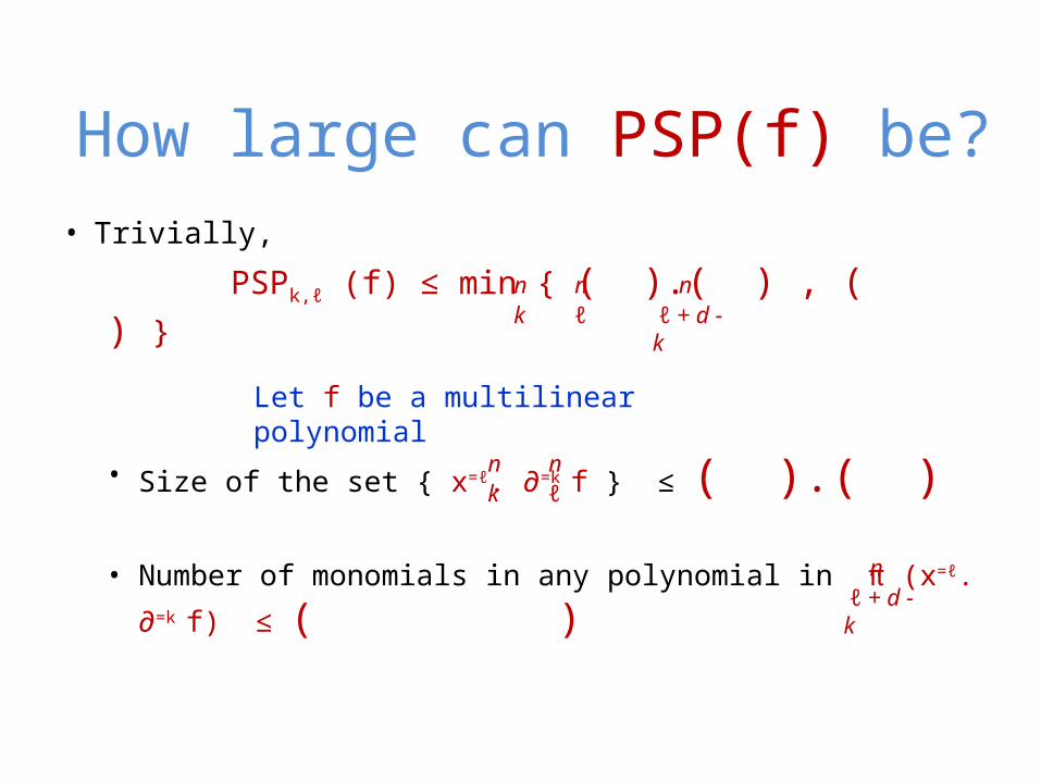
How large can PSP(f) be?• Trivially,
PSPk,ℓ (f) ≤ min ( ).( ) , ( ) nk
nℓ
n ℓ + d - k
How large can PSP(f) be?• Trivially,
PSPk,ℓ (f) ≤ min ( ).( ) , ( ) nk
nℓ
n ℓ + d - k
• Size of the set x=ℓ. ∂=k f ≤ ( ).( )
• Number of monomials in any polynomial in π (x=ℓ. ∂=k f) ≤ ( )
nk
nℓ
n ℓ + d - k
Let f be a multilinear polynomial

How large can PSP(f) be?• Trivially,
PSPk,ℓ (f) ≤ min ( ).( ) , ( )
• Best lower bound for s
s ≥
nk
nℓ
nℓ + d - k
min ( ).( ) , ( ) ( ).( ) m
kn
ℓ + 2kt
nk
nℓ
nℓ + d - k = nΩ(d/t)
After setting k and ℓ appropriately
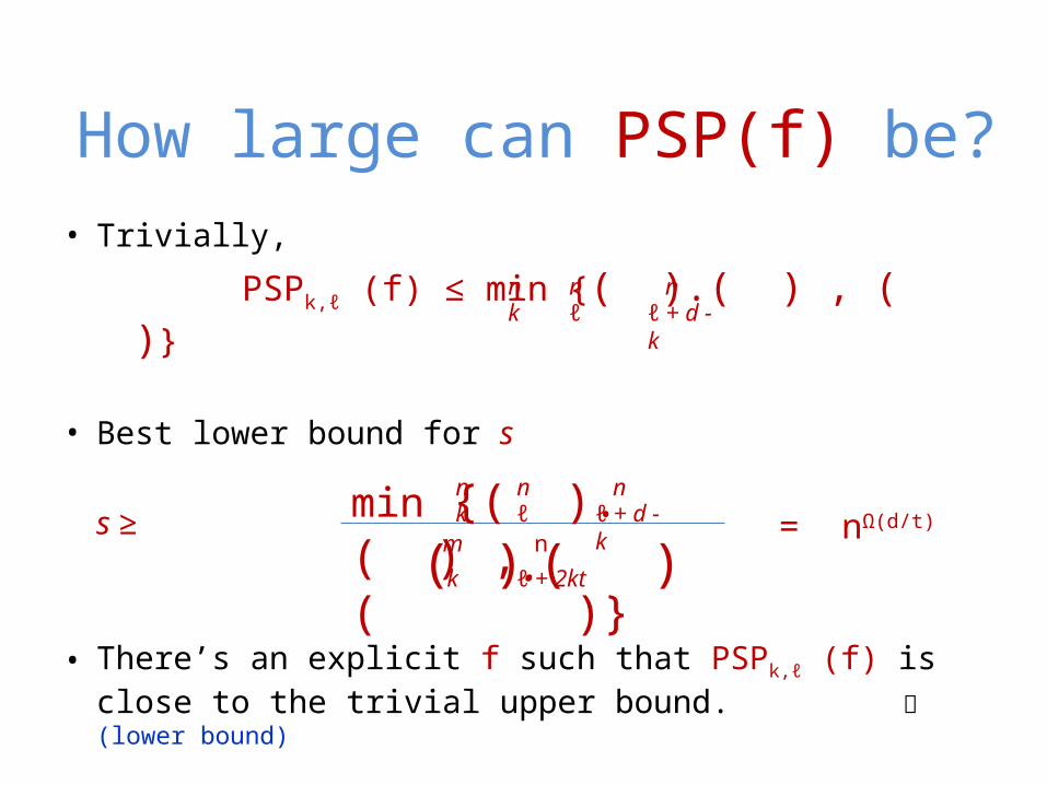
How large can PSP(f) be?• Trivially,
PSPk,ℓ (f) ≤ min ( ).( ) , ( )
• Best lower bound for s
s ≥
• There’s an explicit f such that PSPk,ℓ (f) is close to the trivial upper bound. (lower bound)
nk
nℓ
nℓ + d - k
min ( ).( ) , ( ) ( ).( ) m
kn
ℓ + 2kt
nk
nℓ
nℓ + d - k = nΩ(d/t)

Depth-3 lower bound

Trading depth for homogeneity
Idea: Depth-3 with low bottom fanin
Homogeneous depth-4 with low bottom support
Size = sBottom fanin = t
3
fn
4 (homogeneous)
fn
Size = s . 2O(√d)
Bottom support = t

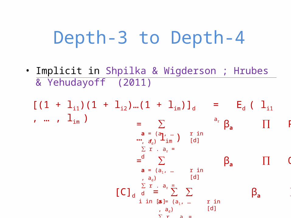
Depth-3 to Depth-4
• Implicit in Shpilka & Wigderson ; Hrubes & Yehudayoff (2011)
C = α1.(1 + l11)(1 + l12)…(1 + l1m) + …. + αs.(1 + ls1)(1 + ls2)…(1 + lsm)
linear formsfield constants

Depth-3 to Depth-4
• Implicit in Shpilka & Wigderson ; Hrubes & Yehudayoff (2011)
C = (1 + l11)(1 + l12)…(1 + l1m) + …. + (1 + ls1)(1 + ls2)…(1 + lsm)
Notation: [g]d = d-th homogeneous part of g
Easy observation: If C = f , which is homogeneous deg d polynomial, then [C]d = f.

Depth-3 to Depth-4
• Implicit in Shpilka & Wigderson ; Hrubes & Yehudayoff (2011)
C = (1 + l11)(1 + l12)…(1 + l1m) + …. + (1 + ls1)(1 + ls2)…(1 + lsm)
[C]d = [(1 + l11)(1 + l12)…(1 + l1m)]d +….+ [(1 + ls1)(1 + ls2)…(1 + lsm)]d
idea: transform these to homogeneous depth-4

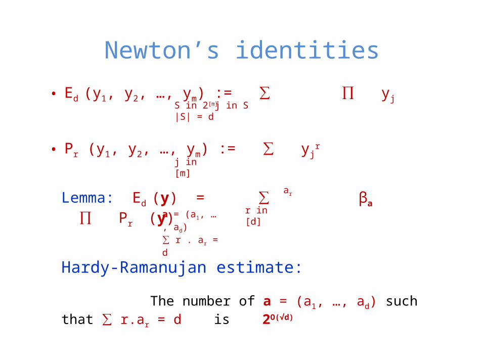
Newton’s identities
• Ed (y1, y2, …, ym) := ∑ ∏ yj
• Pr (y1, y2, …, ym) := ∑ yjr
S in 2[m] |S| = d
j in S
(elementary symmetric polynomial of degree d)
j in [m]
(power symmetric polynomial of degree r)

Newton’s identities
• Ed (y1, y2, …, ym) := ∑ ∏ yj
• Pr (y1, y2, …, ym) := ∑ yjr
S in 2[m] |S| = d
j in S
j in [m]
Lemma: Ed (y) = ∑ βa ∏ Pr (y) a = (a1, … , ad)∑ r . ar = d
r in [d]
ar
e.g. 2y1y2 = (y1 + y2)2 – y12 – y2
2 = P1
2 – P2
field constant
Newton’s identities
• Ed (y1, y2, …, ym) := ∑ ∏ yj
• Pr (y1, y2, …, ym) := ∑ yjr
S in 2[m] |S| = d
j in S
j in [m]
Lemma: Ed (y) = ∑ βa ∏ Pr (y) a = (a1, … , ad)∑ r . ar = d
r in [d]
ar
Hardy-Ramanujan estimate:
The number of a = (a1, …, ad) such that ∑ r.ar = d is 2O(√d)

Depth-3 to Depth-4
• Implicit in Shpilka & Wigderson ; Hrubes & Yehudayoff (2011)
[(1 + li1)(1 + li2)…(1 + lim)]d = Ed ( li1 , … , lim )
= ∑ βa ∏ Pr ( li1 , … , lim ) a = (a1, … , ad)∑ r . ar = d
r in [d]
ar
2O(√d) summands

Depth-3 to Depth-4
• Implicit in Shpilka & Wigderson ; Hrubes & Yehudayoff (2011)
[(1 + li1)(1 + li2)…(1 + lim)]d = Ed ( li1 , … , lim )
= ∑ βa ∏ Pr ( li1 , … , lim ) a = (a1, … , ad)∑ r . ar = d
r in [d]
ar
2O(√d) summands
Suppose every lij has at most t variables, then…

Depth-3 to Depth-4
• Implicit in Shpilka & Wigderson ; Hrubes & Yehudayoff (2011)
[(1 + li1)(1 + li2)…(1 + lim)]d = Ed ( li1 , … , lim )
= ∑ βa ∏ Pr ( li1 , … , lim ) a = (a1, … , ad)∑ r . ar = d
r in [d]
ar
= ∑ βa ∏ Qi,a,r a = (a1, … , ad)∑ r . ar = d
r in [d]
every monomial has support ≤ t
Depth-3 to Depth-4
• Implicit in Shpilka & Wigderson ; Hrubes & Yehudayoff (2011)
[(1 + li1)(1 + li2)…(1 + lim)]d = Ed ( li1 , … , lim )
= ∑ βa ∏ Pr ( li1 , … , lim ) a = (a1, … , ad)∑ r . ar = d
r in [d]
ar
= ∑ βa ∏ Qi,a,r a = (a1, … , ad)∑ r . ar = d
r in [d]
[C]d = ∑ ∑ βa ∏ Qi,a,r a = (a1, … , ad)∑ r . ar = d
r in [d]i in [s]
Homogeneous depth-4 with low bottom support and size s.2Ω(√d)

An explicit family with high PSPk,ℓ

An explicit family of polynomials• Nisan-Wigderson family of polynomials:
NWr := ∑ ∏ xi, h(i)d2 h(z) in F [z],
deg(h) ≤ ri in [d]
identifying the elements of F with 1,2, … , d2d2

An explicit family of polynomials• Nisan-Wigderson family of polynomials:
NWr := ∑ ∏ xi, h(i)d2 h(z) in F [z],
deg(h) ≤ ri in [d]
`Disjointness’ property: Two monomials can share at most r ≈ d/3 variables.
= + + …
d
r r
d2(r+1) monomials

Projected Shifted Partials of NWr
• The set π (x=ℓ. ∂=k NWr) has ( ).( ) elements.
• Every polynomial in π (x=ℓ. ∂=k NWr) is multilinear & homogeneous of degree (ℓ + d – k).
nk
nℓ

Projected Shifted Partials of NWr
• The set π (x=ℓ. ∂=k NWr) has ( ).( ) elements.
• Every polynomial in π (x=ℓ. ∂=k NWr) is multilinear & homogeneous of degree (ℓ + d – k).
• PSPk,ℓ (NWr) = rank (M)
nk
nℓM := ( ).( ) rows
π (x=ℓ. ∂=k NWr)
(0/1)-matrix of coefficients
nℓ + d - k ( ) columns
nk
nℓ

Projected Shifted Partials of NWr
• Because of the `disjointness property’ of NWr , the columns of M are almost orthogonal.
• Hence, B := MT M is diagonally dominant.
• Observe, rank (M) ≥ rank (B) .

Projected Shifted Partials of NWr
• Because of the `disjointness property’ of NWr , the columns of M are almost orthogonal.
• Hence, B := MT M is diagonally dominant.
• Observe, rank (M) ≥ rank (B) .
Alon’s rank bound (for diagonally dominant matrix):
If B is a real symmetric matrix then
rank (B) ≥ Tr (B)2
Tr (B2)

Projected Shifted Partials of NWr
[Main lemma]: Using Alon’s bound and settings r , k and ℓ appropriately,
PSPk,ℓ (NWr) ≥ η. min ( ).( ) , ( )nk
nℓ
nℓ + d - k
small factor

An explicit family in VP• [Kumar-Saraf (2014)] : Showed the same lower bound using
the Iterated Matrix multiplication polynomial, which is in VP

An explicit family in VP• [Kumar-Saraf (2014)] : Showed the same lower bound using
the Iterated Matrix multiplication polynomial, which is in VP
VNP
Circuits (VP)
ABPs
Formulas
Depth-4
exponential separation

An explicit family in VP• [Kumar-Saraf (2014)] : Showed the same lower bound using
the Iterated Matrix multiplication polynomial, which is in VP
VNP
Circuits (VP)
ABPs
FormulasOpen: separation ?
…known in the multilinear setting[Dvir, Malod, Perifel, Yehudayoff (2012)]

An explicit family in VP• [Kumar-Saraf (2014)] : Showed the same lower bound using
the Iterated Matrix multiplication polynomial, which is in VP
VNP
Circuits (VP)
ABPs
Formulas
Open: separation ?
…improve nΩ(√d) to nω(√d)

Some other open questions
1. Prove a nΩ(√d) lower bound for general depth-3 circuits (i.e. without the low bottom fanin restriction).

Some other open questions
1. Prove a nΩ(√d) lower bound for general depth-3 circuits.
2. Prove a nΩ(√d) lower bound for homogeneous depth-5 circuits. [open problem in Nisan & Wigderson (1996)]
(2) (1)

Some other open questions
1. Prove a nΩ(√d) lower bound for general depth-3 circuits.
2. Prove a nΩ(√d) lower bound for homogeneous depth-5 circuits.
3. Prove a nΩ(d) lower bound for multilinear depth-3 circuits. (current best is 2Ω(d) )
…interestingly, one can get this using PSP measure

Some other open questions
1. Prove a nΩ(√d) lower bound for general depth-3 circuits.
2. Prove a nΩ(√d) lower bound for homogeneous depth-5 circuits.
3. Prove a nΩ(d) lower bound for multilinear depth-3 circuits.
4. A separation between homogeneous formulas and homogeneous depth-4 formulas.

Some other open questions
1. Prove a nΩ(√d) lower bound for general depth-3 circuits.
2. Prove a nΩ(√d) lower bound for homogeneous depth-5 circuits.
3. Prove a nΩ(d) lower bound for multilinear depth-3 circuits.
4. A separation between homogeneous formulas and homogeneous depth-4 formulas.
5. A separation between homogeneous formulas and multilinear homogeneous formulas.
…exhibiting the power of non-multilinearity

Some other open questions
1. Prove a nΩ(√d) lower bound for general depth-3 circuits.
2. Prove a nΩ(√d) lower bound for homogeneous depth-5 circuits.
3. Prove a nΩ(d) lower bound for multilinear depth-3 circuits.
4. A separation between homogeneous formulas and homogeneous depth-4 formulas.
5. A separation between homogeneous formulas and multilinear homogeneous formulas.
Thanks!