Advances in Powertrains and Automotives, 2015, Vol. 1, No. 1, 12-23 Available online at http://pubs.sciepub.com/apa/1/1/2 © Science and Education Publishing DOI:10.12691/apa-1-1-2

Low Noise Intake System Development for Turbocharged I.C. Engines Using Compact High

Frequency Side Branch Resonators

Sabry Allam*

Automotive Technology Department, Faculty of Industrial Education, Helwan University, Cairo, Egypt *Corresponding author: allam@kth.se

Received April 20, 2015; Revised May 04, 2015; Accepted May 19, 2015

Abstract Turbochargers have become common in passenger cars as well as commercial vehicles. They have an excellent mechanism to effectively increase fuel efficiency and engine power, but they unfortunately cause several noise problems. Its noise are mainly classified as structure-borne noises, generated from the vibration of rotating shaft modules (cartridges), and air-borne noises, from air flow inside turbochargers or their coupling ducts. In this study an attempt to reduce the pulsation noise generated from the compressor wheels, whose frequency is the same as the whine noise is presented. This attempt is based on using the compact high frequency side branch resonators to develop low intake noise system. The design of such system, which is mainly based on the developed 1D linear acoustic theory and theoretical investigations to use more than one resonator connected to the main duct in series and/or in parallel are introduced. An optimization strategy to choose the appropriate resonator axis offset is presented. In case of complex unsymmetrical geometry in real resonators, a 3 D finite element is used. The presented models are validated via comparison with the measured results at room temperatures. The validated models are used to improve the acoustic performance of the real resonators. Based on the developed models and the optimization results, the internal design of resonators improves its acoustic performance; the serial arrangements increase the damping at the same peak frequency while the parallel arrangements make it wider. The amount of extra damping added to the intake system depends on the resonators geometry and their axis offset which can be around 50 dB at the peaks, and 30 dB between peeks at normal operating engine conditions. Extra improvement to the intake system noise reduction can be achieved by redesigning and optimizing the entire system with used resonators under both space and shape constrains.

Keywords: Engine Intake system, noise reduction, Turbocharger, resonators, serial and parallel arrangement, 1D linear frequency domain, 3D FEM Simulation, shape optimization

Cite This Article: Sabry Allam, “Low Noise Intake System Development for Turbocharged I.C. Engines Using Compact High Frequency Side Branch Resonators.” Advances in Powertrains and Automotives, vol. 1, no. 1 (2015): 12-23. doi: 10.12691/apa-1-1-2.

1. Introduction Turbochargers use engine exhaust gas energy to

compress more fresh air into cylinders, aiming to improve combustion efficiency. A turbocharger can increase engine power and torque by 30% against a naturally aspirated engine of the same size, it can also greatly improves fuel economy and emission. Therefore turbocharging technologies are more and more widely used on engines, especially on those downsized [1,2,3]. However, turbochargers have a number of negative impacts on engine and vehicle evaluation and performance, one of the issues is turbo noise.

The intake noise of naturally aspirated automobile is normally induced by firing of an engine or by flow separation [3]. The piston pumping generates pressure pulsation travel upstream through different wall components and emitted either through the wall as shell

noise or through the intake orifice as flow generated noise. The amplitude of the intake noise source can be high enough to make it a significant contributor to the interior noise especially when it matches the acoustic resonance at certain frequencies due to the length of the intake system.

Turbochargers often add noise with much higher frequency due to the high speed revolution of the compressor wheel and generally higher flow velocity.

There are different types of turbo noise due to different mechanisms such as rotor vibration, airflow pulsation and oil film oscillation etc. For small turbochargers rotating at speeds up to 300,000 rpm which are normally used in passenger vehicles, the so-called synchronous noise, which is identical to turbo speed is biggest issue to achieve the customer satisfaction.

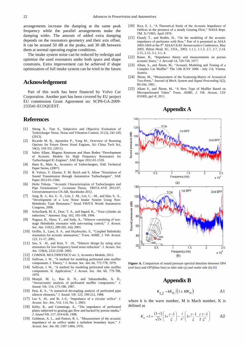
The turbo synchronous noise lies between 1000 to 5000 Hz, and it is much higher than that of engine noise, it can be easy detected in car cab [4,5,6], and sounds very sharp and annoying see for example Appendix A.

Advances in Powertrains and Automotives 13

Turbo synchronous noise can be generated by two mechanisms. The first is the residual unbalances of the rotor, which causes the entire turbocharger and connecting pipework to vibrate and radiate noise. Therefore rotors must be properly balanced. The other mechanism is pressure pulsation that is caused by the non-uniformity between impeller blades and as well as by the eccentric motion of the entire impeller in charged air, which excite the pipe and intercooler downstream the compressor outlet to vibrate and radiate noise. Thus reduction of the synchronous noise becomes very argent for turbocharger manufacturers and this the main aims of this paper. One way to reduce pulsation-induced turbo synchronous noise as well as to reduce the tonal noise is to install a suitable resonator just downstream the compressor outlet [3,7,8].

Several types of resonators are commonly used by directly connecting to the engine induction system which use gas inertia and compressibility, to build an acoustic filter to block the noise transfer from source to the connected pipe system. However, the problem usually has to be solved with the range of a number of important parameters strongly restricted.

If the resonant frequency of the resonator can be tuned dynamically or statically to the noise frequency, the resonator will work for a wide range of frequencies [9]. Due to the complexity of the dynamic method, the easiest and more applicable way is to tune the resonant frequency of the resonators statically, which can be done, using an array of resonators. This array can be arranged in series to give high damping, and also can also be parallel for wide frequency range and combination of both inside one cavity can be used, it will be capable of suppressing the intake and exhaust noise using one resonator [3,10,11].

Considering the modelling of sound transmission in intake systems, there are different types of simulation approaches that can be used based on, non-linear time domain and linear frequency domain models [8,9,10,11].

Based on the liner frequency domain, an attempt to develop efficient acoustic models to be used to design low noise intake system for turbocharged IC-engine will be presented in this paper. Throughout, this study, a 1D acoustic model to study compact resonators, which used to control turbo generated noise over a wide frequency range is developed, a combination of resonators in series and parallel arrangements inside a single cavity or multi cavities to cover a wide frequency range from 1 to 2 KHz have been investigated and optimized aiming at understanding the acoustic interaction between the cavities and improving the acoustic performance of the inter system. A 3D Finite Element COMSOL Multiphysics [12] will be also built and used in case of complex resonators to be able to catch the 3D acoustic effect for the proposed resonators. Comparison between the proposed models and the measured results at room temperature will be also presented.

1.1. Structure of the Paper This paper describes the design of compact side branch

resonators which is mounted in the I.C Engine intake system close to the compressor outlet to reduce turbo synchronous noise. Analytical investigation of the of sound transmission through resonators, optimization process to choose the best configuration and position are

presented in section 2, an application to real case is also introduced in the same section. Based on the results it has been shown that the 3D effect must be included using FEM and it is introduced in section 3. Summary of the measurement procedure and the tested objects are presented in section 4. Employments of the analytical and numerical methods to determine the acoustic performance of the required resonators are presented and compared with the measured results in section 5. In section 6 some conclusions and recommendations for future work are presented.

2. Theoritical Modelling

2.1. Sound Transmission through Side Branch Resonators

Resonator reduces noise by an impedance mismatch that causes reflection of the incident acoustic energy and attenuation in the resonators neck. When a resonator is attached to a duct by a side branch, as depicted in Figure 1, the basic assumption is that plane waves propagate in the duct and the reflected waves from downstream are eliminated by using an anechoic termination in the absence of mean flow.

Figure 1. Side branch resonators in a duct. A & B incident, and reflected wave amplitudes, S & L cavity cross sectional area and height, S1 & S2 cross sectional area of upstream and downstream duct, and D & Ln are the neck diameter and length

Considering effects of grazing flow, if the mean flow velocity is less than M ≤ 0.1, where M is the Mach number, this effect can be neglected.

Based on the plane wave theory and with the reference to Figure 1, the sound pressure (p) and volume velocity (q) can be expressed as

1 2

1 2

e

e e

i K x i K xi i i

i K x i K xii i i

p A e B

Sq A B

cρ

−

−

= +

= −

(1)

14 Advances in Powertrains and Automotives

Where, A and B are incident, and reflected wave amplitude, i=1, 2, and 3, K1, K2 are the complex wave numbers and they are defined in Appendix B. Using x=0 in equation 1, the incident and the reflected amplitudes can be written as

( ) ( ) ( )

1 1 2 2 3 3

1 1 11 1 1 2 2 2 3 3 3

A B A B A B

Z A B Z A B Z A B

+ = + = +

− = − + − (2)

The rigid boundary condition at the end of the side-branch forces the volume velocity to vanish i.e. q3=0 gives

1 23 3e e 0i K x i K xA B− − =

(3)

With the help of the nonreflecting boundary condition at the duct outlet, B2=0. Combining equations (2), and (3) yield

( )

( )

31 21

1 1

2 2 31 23

e 112 2

2 e 1

i K K L

K K L

ZA ZA Z

Z

+

+

− = + + +

(4)

If the impedance Zi (i=1,2, and 3) can be defined as Zi=ρoco/Si, the transmission coefficient τ=A1/A2 can be written as

( )

( )

31 23

2

1 31 21

e 112 2

2 e 1

i K K L

K K L

SSS

S

τ

+

+

− = + + +

(5)

If K1=K2=k, S2=S1, τ can be simplified as

2 33

2 31

e 1

1

2 e 1

i k L

i k L

S

Sτ

−

= +

+

(6)

The transmission loss(TL) can be calculated using

21010TL log τ= (7)

To drive the preferable 2-port matrix, with the assumption of incompressible mean flow and applying conservation of momentum and mass across the side-branch (with an opening assumed to be much smaller than a wavelength), equation (2) can be written as

1 2

1 2

ˆ ˆ 0ˆ ˆ ˆin

p pq q q

− ≈ = +

(8)

where the acoustic pressure is assumed to be approximately constant across the side-branch. This implies that acoustic near fields and flow induced losses are neglected. Inserting the definition of impedance ( ˆ ˆ /in in tq p Z= ) into the above equations gives

1 0

1 1T

Zt

=

(9)

The TL can be calculated as [3]

1

2

21

1 410 log10 2

12 1 2211 1 21

2 2

M ZinM Zout

TLT Z T

T Z TZ Z

+

+=

× + + +

(10)

Substituting the T matrix elements from equation (8) in equation (9), the final form can be calculated and it will be equal to the same in equation (7) in case of without flow.

For the case of a quarter-wave resonator (QWR) that is shown in Figure 1. (a), the input impedance can be obtained from the straight pipe transfer-matrix, by assuming a rigid termination. This gives the input impedance at (M =0)

( )31

coto ot

c

cZ i kL

Sρ

= − (11)

Where, M=U/co is the flow Mach number, U is flow speed, co is the sound speed.

The transmitted pressure is infinite small when 2 2e

i k Lnπ= , where n= 1, 3, 5,…, thus

24r of nc L= (12)

where fr is the resonance frequency. On the other hand, to yield a TL peak at a certain frequency, the length of the side-branch cavity is required to be L2 = nco/4fr.

In case of helmholtz resonator (HR) as shown in Figure 1(b), Z Z Zt ch= + , are the total impedance, Zh hole impedance and cavity impedance respectively. The normalized cavity impedance can be calculated as

( )cotZ i kLc i= − , where, Li is defined as the cavity height. More details about the hole impedance will be presented in the following text. The expression for the resonance frequency of a HR is

f2

Sc nr V Lc nπ

= (13)

where, Sn is the cross-sectional area of the neck, co is the speed of sound in a gas, Ln is the length of the neck and Vc is the static volume of the cavity and it can be calculated as

( )

2V 22

c Scc

f Lr cπ= (14)

2.2. Wall Impedance In spite of this large number of publications for the wall

impedance model see as examples [13-21] a single verified global model does not exist. So for circular holes, it is decided to depend on the formula presented by Bauer [22] that was verified by Allam and Åbom [23] to calculate transmission loss data for simple straight through and cross flow and complicated mufflers. The normalized impedance of a perforate with circular holes combined grazing and through flow can be written as

Advances in Powertrains and Automotives 15

0.381

0 0

1.15int

Mt go hZh c C dD h

M jkb t F FhC CD D

µρ ω

ρ σ σ

δ δσ σ

= + + +

+ + × ×

(15)

where Zh is the normalized impedance of the perforate, µ is the dynamic viscosity, σ is the perforate porosity and it equaled to one in case of a single hole, M g is the grazing

flow Mach number, Mb is the bias (through) flow Mach number, CD is the orifice discharge coefficient, ht is the wall thickness and hd is the hole diameter. The factor δ is the acoustic end correction for both side of the hole and put equal to 0.62dh and Fδ is the flow effect on acoustic reactance assumed to be 0.38 according to Rice [20]. For slit like hole, the impedance formula presented in the Appendix C is used.

2.3. Serial Arrangement If more than one resonator are connected in serial and

used together, the transfer matrix can be written as

. . ....1 2 3T T T TNT = (16)

where N, is the number of the elements in the system (resonators and any other acoustic element in the system, pipe, muffler, etc..). T1, T3 are the transfer matrices for the two resonators and T2 is the pipe transfer matrix.

P1

q1 PN qN

…..

X=0 X=L

X=0 X=L

PN qN

P1 q1

AN

A1

B1 Zeq

Z1 Z2

Zduct Zduct

ZN ….

qN q1

P1 PN

Z1 Z2 ZN

P1 q1

PN qN

Z1 Z2 Z3

…..

X=0 X=L S1 S2 SN

Figure 2. Serial resonator arrangement representation: (a) Quarter wave resonator, (b) Helmholtz resonator, (c) Equivalent circuit, (d) Electric circuit

2.4. Parallel Arrangement With refrence to Figure 3, The transfer matrix for

parallel arrangement can be written as

1 0

1T Zeq=

(17)

P1 q1

P2 q2

Z1

Z2

Lx

S1 S2 hc2

hc1

W2

W1

Figure 3. Serial resonator arrangement representation

The equivalent impedance Zeq for a parallel arrangement is obtained as follows:

1 1 1.....

1 2Zeq Z Z Ztnt t

= + +

(18)

Considering a number (N) of identical resonators in parallel, the transfer matrix between point 1 and point 2 can be written as

1 01

TN Zt

=

(19)

Figure 4 and Figure 5 illustrate the effect of the serial and parallel arrangement on the resonators acoustic performance. Regarding the change of TL when the number of resonators is increased, the serial identical arrangement mainly increases the magnitude of TL rapidly at the same resonance frequency while the parallel arrangement increases the magnitude of TL and the bandwidth. These characteristics together give the resonator array high TL in a wide frequency band. In this sense, a resonators or silencer can be designed by using multiple array of resonators having different resonance frequencies, which are included in the target frequency band.

1000 1200 1400 1600 1800 20000

10

20

30

40

50

60

70

80

90

100

Frequency (Hz)

Tra

nsm

issio

n L

oss

(dB

)

S QWR, M=0

N=1N=2N=3N=4

Figure 4. TL versus frequency using an array of resonators in a serial arrangement

16 Advances in Powertrains and Automotives

1000 1200 1400 1600 1800 20000

5

10

15

20

25

30

35

40

45

50

Frequency (Hz)

Tra

nsm

issio

n L

oss

(dB

)P QWR, M=0

N=1N=2N=3N=4

Figure 5. TL versus frequency using an array of resonators in a parallel arrangement

2.5. Serial Arrangement Application An application of the serial arrangments on real

compact side branch resonator is shown in Figure 6. It can be seen that the the presented 1D model give acceptable results, where the resonance frequencies and it maximum values are picked. But there are same shift at high frequecy and in case of flow due to the complixity of the resonators chamber which bring 3D effect.

Figure 6. Transmission loss versus frequency for real resonator in serial arrangement

2.6. Axis Offset Optimization To study the effect of axis offset in case of serial

arrangement on the acoustic performance of QWR that are

shown in Figure 7, where 2 QWR are connected to a pipe from one side or from two sides and all dimensions are listed below, numerical maximization to the transmission loss is needed.

Figure 7. Constructer drawing of serial arrangement used in the illustration. L1=0.042, L2=0.059, S1=0.002 m2, S2=0.002 m2, W1=0.0138 m, W2=0.0106 m, pipe diameter 0.05 m

To maximize the transmission loss (TL), the minimal value of -f(X) is planned and proceeded. Minimize F(X) = -f(X) is the Objective function, where ( )( ) 1F X TL X= , where X1 is design variables (axis offset).

1000 1200 1400 1600 1800 20000

10

20

30

40

50

60

Frequency (Hz)

Tra

nsm

issio

n L

oss

(dB

)

2 S QWR M=0.0

OptimizationFrequency

Range

OptimizedResults

PossibleSolutions

Figure 8. Sound transmission loss versus frequency using 2 QWR in serial arrangement during the optimization process. Lx=0.0201 m is the optimum choice

The transmission loss was evaluated, by using plane wave analysis, at increments of 5 Hz over a frequency range of 1200-1800 Hz. The resulting objective function is therefore

1

1( ) ( )N

TL f TL fNN

= ∑ (20)

Advances in Powertrains and Automotives 17

where, f is the frequency (Hz) and NN is the number of frequency point. The results of such optimization process are shown in Figure 8 and the optimum TL value is obtained at Lx=0.0201 m.

2.7. General Arrangement To take the binifit of both serial and parallel

arrangemets, a series of parallel arrangement an be used which can be presented as

..1 0 1 0

. . ..1 1 1 11 2

T TNTubeZ Zt tT =

(21)

where, Zt1 is the equaivlent impedance as shown in equation (17) of the parallel arrangments and Zt2 is the impedance of the resonator 3 and is defined in the test after equation (9).

Figure 9. The coupling effect between two sub-chambers C1 and C2

Based on equation 21, the overall TL of the system exhibits a combined behavior that superposes the TL peaks provided by the two resonators in the non-overlapping frequency range. This indicates that designing a resonator by cascading different sub-chambers can potentially achieve a broadband attenuation performance, provided that the sub-chambers are properly designed and optimized to be effective in different frequency bands.

The axis offset or the distance between the two parallel resonators in a serial arrangement can be chosen numerically to achieve the best acoustic performance of the resonator which is performed using equations (10), (17), (21), and (22). The optimum results which is shown

at Lx =0.0282 and all the other possible solutions are presented in Figure 11.

Figure 10. Transmission loss versus frequency for general arrangement. (a) M=0, (b) M=0.10

1000 1200 1400 1600 1800 20000

10

20

30

40

50

60

70

Frequency (Hz)

Tra

nsm

issio

n L

oss

(dB

)

M=0

PossibleSolutions

OptimizedResults

OptimizationFrequency

Range

Figure 11. Sound transmission loss versus frequency using 2 parallel QWR in serial arrangement during the optimization process. Lx=0.0282 m is the optimum choice

18 Advances in Powertrains and Automotives

3. FE Model Summary In order to make a complete model to deal with

complex shapes a 3D acoustic FEM approach was chosen. The Mach-number in an intake or exhaust pipe is normally less than 0.3 which means that inside a resonator /mufflers where the flow has expanded the average Mach-number is normally much smaller than 0.1. Therefore one can expect convective mean flow effects on the sound propagation to be small and possible to neglect. The main effect of the flow for a complex resonator and perforated muffler is the effect on the perforate and hole impedances.

For the predictions the 3D FEM software COMSOL MULTIPHYSICS [12] has been used. Assuming a negligible mean flow the sound pressure p will then satisfy the Helmholtz equation:

21

0o o

k pp

ρ ρ∇ ⋅ ∇ − + =

q (22)

where, k = 2πf /co is the wave number, ρo is the fluid density and co is the speed of sound. The q term is a dipole source term corresponding to acceleration/unit volume which here can be put to zero. Using this formulation one can compute the frequency response using a parametric solver to sweep over a frequency range. Through the COMSOL MULTIPHYSICS software different boundary conditions are available; sound-hard boundaries (walls), sound-soft boundaries (zero acoustic pressure), specified acoustic pressure, specified normal acceleration, impedance boundary conditions, and radiation boundary conditions.

The boundary conditions used in this paper include, sound-hard boundaries ( ( ). n 0op ρ∇ − = ), where, n is the unit normal pointing into the fluid domain and radiation boundary conditions at the inlet and outlet. The boundary condition at the inlet involves a combination of incoming and outgoing plane waves:

( )( ) ( )

0 0

.00

k r

1.2

1 .2

n

k n

T

ikT

o

p ip ik pk

pi p ik ek

ρ ρ

ρ−

∇ + + ∆

= ∆ + −

(23)

In this equation, p0 represents the applied outer pressure, ΔT is the boundary tangential Laplace operator, and i equal the imaginary unit. This boundary condition is valid as long as the frequency is kept below the cutoff frequency for the second propagating mode in the tube. At the outlet boundary, the model specifies an outgoing plane wave:

1n. 0

2o o

k ip i p pTkρ ρ

∇ + + ∆ = (24)

Also, a specified normal acceleration ( n. ( 1 ).o p anρ− − ∇ = ) is used, where the continuity of normal nu velocity combined with: ( ) /1 2 hp p Z un− = , where Zh is the perforate impedance and 1 and 2 denotes the acoustic pressures on each side of the perforate, was used. It can be noted that the use of continuity of normal velocity is consistent with our assumption that mean flow effects are small and can be neglected.

The wave numbers and mode shapes through a cross section of the chamber are found as the solution of a related eigenvalue problem:

( ) ( )22

2,

. , 0o oo

p y z kx p y zc

ωρ ρρ

∇∇ − − − =

(25)

For a given angular frequency ω = 2π f, only modes such that 2

xk is positive can propagate. The cutoff frequency of each mode is calculated as

2 2 2

2

c kxf jω

π

−= (26)

Assuming nonreflecting B.C. on the outlet side. The transmission loss (in dB) of the acoustic energy can be defined as:

10 ,10PITL LogPo

=

(27)

Here PI and PO denote the incoming power at the inlet and the outgoing power at the outlet, respectively. You can calculate each of these quantities using an integral over the corresponding surface as

,

2

2

2

| |2

o

o o

outo o

o oA

pP dAI IcAp

P dAc

ρ

ρ∂

= ∫∂

= ∫ (28)

where, p0 represents the applied inlet pressure amplitude and pout is the calculated pressure at the outlet.

4. Summary of Experimental Procedure Experiments were carried out at room temperature

using the flow acoustic test facility at the Marcus Wallenberg Laboratory (MWL) for Sound and Vibration research at KTH. The test duct used during the experiments consisted of a standard steel-pipe with a wall thickness of 3 mm, duct inner diameter di=51 mm and overall length of around 7 meters. Four loudspeakers were used as external acoustic sources, and they were divided equally between the upstream and downstream side as shown in Figure 12. The distances between the loudspeakers were chosen carefully to avoid any pressure minima at the source position. Six flush mounted condenser microphones (B&K 4938) were used, three upstream and three downstream of the test object for the plane wave decomposition, the microphone separations are chosen to fulfill the frequency ranges of interest from 30 to 3000 Hz.

All measurements are performed using the source switching technique [24] and the TL is calculated based on the measured results. The flow speed was measured upstream of the test section using a small pitot-tube connected to an electronic manometer SWEMA AIR 300 fixed at a distance of 1000 mm from the upstream loudspeakers section. The test objects are connected to the main duct via suitable conical section and its effect on the measured results is removed through the analysis.

Advances in Powertrains and Automotives 19

Figure 12. Measurement set up used during the T- Port Experimental procedure

4.1. Case Studies

4.1.1. Case 1: Converting the geometric model of a resonator to an

acoustic model is an important step in linear acoustic modeling and with the reference to Figure 13, it can be seen that resonator mainly consists of two compact side branch resonators with slit opening and one circular pipe in between. The dimensions of the elements are listed below.

Figure 13. Dimensions of the resonator ( Case 1). Neck Length 0.002 m, Sc1 =10.6e-4 m2, Sc2=19e-4m2,S1=S2=1.9e-3, L1=0.042m, L2=.059m

4.1.2 Case 2: It is divided into three Helmholtz resonators and two

expansion chambers connected with each other as shown in Figure 14. The thickness of the inner pipe is considered as the neck length of the resonators while the opening area is treated as the neck area. The chamber which is connected with the inlet pipe has an outlet pipe extension. Also, the divergences are taken into account during the modeling.

Figure 14. Photo and dimensional details of test object 2

20 Advances in Powertrains and Automotives

4.1.3 Case 3: As shown in Figure 15, Case 3 consists of 7 resonators

are arranged in parallel and series. The dimensions of the chambers are listed below.

Figure 15. Photo and dimensional details of test object 3. (b) Chamber wall thickness 3 mm, chamber main width 17.8, 21.7, 15, 14.4, 14, 15.2,20 mm, inner diameter 34mm

5. Results and Discussion Figure 16 shows the comparison between measured and

simulated results using 1D simulation with the help of the slit like hole impedance model presented in Appendix C. It can be seen from the results there is a good agreement for the no flow case while the agreement is less good in case of flow. This can be due to the un-symmetry of the second chamber of the resonator and can be also due to the uncertainty in the end correction especially with flow [3].

0 200 400 600 800 1000 1200 1400 1600 1800 20000

5

10

15

20

25

30

35

40

45

50

Frequency (Hz)

TL (d

B)

Measured at M=0.00Predicted at M=0.00Measured at M=0.05Predicted at M=0.05Measured at M=0.10Predicted at M=0.10

Figure 16. Measured and predicted TL at different flow speed.

It can also be stated that the quality of the simulation depends on the choice of the impedance model. The choice of the impedance model affects the resonance peak

frequency and strength, it means that if the hole impedance model presented in equation (15) is used instead of correct impedance model presented in Appendix C, the simulation results will be shifted.

Figure 17 (b), shows the improvement in the simulation when FEM is used, but there are also some deviations especially with flow due to neglecting convective effect and the uncertainty in the end correction used with the impedance model.

Figure 17. Measured and predicted TL using FEM at different flow speed

To take the advantage of the parallel effect and serial effect at same time, the first resonator in the test object is divided into 2 and 4 small resonator consequently as shown in Figure 18(a). Its effect on the TL is shown in Figure 18 (d). Even if the volume of the first resonator is still constant, dividing it to four small parallel resonators makes the TL curves wider that improves the performance of the resonator. It can be also, from Figure 18 (b) and (c) seen that the first peak comes from the second resonator and the second peak comes from the first resonator, it be also seen that the changes mainly occurs at the second peak but if the second resonator is divided the TL curve will be even wider.

It has been check the possibility of using the 1D theory to model the complex geometry which is presented by Resonator case study 2 shown in Figure 14, it has be found that using 1D model one can predict the TL at the peak and the resonance frequency but there is a mismatch between the measured and simulated results away from the peak. So, it has been decided to use a 3D FEM solution. Big improvements have been add to simulated results using the 3D FEM compared with the measured

Advances in Powertrains and Automotives 21

data as shown in Figure 19 (b), but the mismatch can be seen as well due to the simplification in the CAD drawing that is used in through simulation and is shown in Figure 12(a).

Also, it can be due to the detail geometry of the hole which has a certain inclination, which is not included in the impedance model.

Figure 18. Effect of parallel arrangement on real resonator acoustic performance

Figure 19. Measured and predicted TL using FEM at different flow speed for Case study 2

Extra improvements have been added to the simulation of the test case 3 that is shown in Figure 14 when full CAD drawing is imported and 513000 elements with fine mesh and relative tolerance 1e-6 are used, that give very good agreement with the measurement as Figure 20.

0 500 1000 1500 20000

5

10

15

20

25

30

35

40

45

50

Frequency (Hz)

Tra

nsm

issio

n L

oss

(dB

)

Case3 Measured at M=0.00Case 3 Measured at M=0.10Case3 Predicted at M=0.00Case3 Predicted at M=0.10

Figure 20. Measured and predicted TL using FEM at different flow speed for Case study 3. The convergence analysis has been checked using finer mesh and higher number of elements and it gave the same TL results

6. Conclosion and Future Work In this paper, the acoustic behavior of the sound

transmission in simple and complex side branch resonators has been characterized, both experimentally and theoretically aiming at improving the acoustic performance of the I.C. Engine intake system.

Throughout this paper, two different analytical approaches have been developed; the first approach is based on 1D model and while the second is based on 3D FEM. The first approach is used though the resonator’ arrangements, demonstration and optimization while the second is used to study the real complex resonators where the 3D effect is important. The 1D model works fine with simple geometries and it is still useful in the early stage design to get an overview of the resonance frequencies and maximum damping. The second approach is the 3D FEM, which gives better results but is very sensitive to the object dimensions, so it requires an accurate input in both CAD drawings and the boundary conditions.

By rearrange the internal design of existing resonators, it will improve its acoustic performance; the serial

22 Advances in Powertrains and Automotives

arrangements increase the damping at the same peak frequency while the parallel arrangements make the damping wider. The amount of added extra damping depends on the resonators geometry and their axis offset. It can be around 50 dB at the peaks, and 30 dB between them at normal operating engine conditions.

The intake system noise can be reduced by redesign and optimize the used resonators under both space and shape constrains. Extra improvement can be achieved if shape optimization of full intake system can be tried in the future.

Acknowledgement Part of this work has been financed by Volvo Car

Corporation. Another part has been covered by EU project EU commission Grant Agreement no: SCP8-GA-2009-233541-ECOQUEST.

References [1] Sheng X., Tian S., Subjective and Objective Evaluation of

Turbocharger Noise, Noise and Vibration Control, 33 (3), 241-245, (2013).

[2] Ricardo M. B., Apostolos P., Yang M., Overview of Boosting Options for Future Down Sized Engines, Sci China Tech Sci, 54(2), 318-331, (2011).

[3] Sabry Allam, Magnus Knutsson and Hans Boden “Development of Acoustic Models for High Frequency Resonators for Turbocharged IC-Engines”. SAE Paper 2012-01-1559.

[4] Hans R., Mats A., Acoustics of Turbochargers, SAE Technical Paper Series, (2007).

[5] R. Veloso, Y. Elnemr, F. M. Reich and S. Allam “Simulation of Sound Transmission through Automotive Turbochargers”. SAE Paper 2012-01-1560.

[6] Heiki Tiikoja. ‘‘Acoustic Characterization of Turbochargers and Pipe Terminations’’. Licentiate Thesis, TRITA-AVE 2012:07, Universitetsservice US-AB, Stockholm 2012.

[7] Jung, B, -I., Ko, U. -S., Lim, J. -M., Lee, C. –M., and Han, S, -S., “Development of a Low Noise Intake System Using Non-Helmholtz Type Resonator,” Seoul FISITA World Automotive Congress, 2000.

[8] Schuchardt, M. E., Dear, T. A., and Ingard, K., ‘‘Four-cylinder air induction,’’ Automot. Eng. 102, 105-108, 1994.

[9] Nagaya, K., Hano, Y., and Suda, A., “Silencer consisting of two-stage Helmholtz resonator with auto-tuning control,” J. Acoust. Soc. Am. 110(1), 289-265, July 2001.

[10] Griffin, S., Lane, S. A., and Huybrechts, S., “Coupled Helmholtz resonators for acoustic attenuation,” Trans. ASME, J. Vib. Acoust. 123, 11-17, 2001.

[11] Seo, S. –H., and Kim, Y. –H., “Silencer design by using array resonators for low-frequency band noise reduction”. J. Acoust. Soc. Am. 118(4), 2332-2338. 2005.

[12] COMSOL MULTIPHYSICS ver. 5, Acoustics Module, 2015. [13] Sullivan, J. W., “A method for modeling perforated tube muffler

components. I. Theory,” J. Acoust. Soc. Am. 66, 772-778, 1979. [14] Sullivan, J. W., “A method for modeling perforated tube muffler

components. II. Application,” J. Acoust. Soc. Am. 66, 779-788, 1979.

[15] Munjal, M. L., Rao K. N., and Sahasrabudhe, A. D., “Aeroacoustic analysis of perforated muffler components,” J. Sound. Vib. 114, 173-188, 1987.

[16] Peat, K. S., “A numerical decoupling analysis of perforated pipe silencer elements,” J. Sound. Vib. 123, 199-212, 1988.

[17] Lee S. -H., and Ih, J.-G. “Impedance of a circular orifice” J. Acoust. Soc. Am., Vol. 114, No. 1, 2003.

[18] Kirby, R., and Cummings, A., “The impedance of perforated plates subjected to grazing gas flow and backed by porous media,” J. Sound Vib. 217, 619-636, 1998.

[19] Goldman, A. L., and Panton, R. L. “Measurement of the acoustic impedance of an orifice under a turbulent boundary layer,” J. Acoust. Soc. Am. 60, 1397-1404, 1976.

[20] Rice, E. J., “A Theoretical Study of the Acoustic Impedance of Orifices in the presence of a steady Grazing Flow,” NASA Rept. TM. X-71903, April 1976.

[21] Elnady T., and Bodén, H., “On the modeling of the acoustic impedance of perforates with flow,” Part of it presented as AIAA 2003-3304 at the 9th AIAA/CEAS Aeroacoustics Conference, May 2003, Hilton Head, SC, USA., 2003. 1.1.1, 1.1.3, 2.7, 2.7, 2.14, 2.15, 2.15, 3.1, 3.1, 4.

[22] Bauer, B., “Impedance theory and measurements on porous acoustic liners,” J. Aircraft 14, 720-728, 1977.

[23] Allam, S., and Åbom, M., “Acoustic Modeling and Testing of a Complex Car Muffler” The 13th ICSV 2006 - July 2-6, Vienna, Austria.

[24] Åbom, M., “Measurement of the Scattering-Matrix of Acoustical Two-Ports,” Journal of Mech. System and Signal Proceeding 5(2), 89-104, 1991.

[25] Allam S., and Åbom, M., “A New Type of Muffler Based on Microperforated Tubes” Trans. ASME, J. Vib. Acoust, 133/ 031005, pp1-8, 2011.

Appendix A

Figure A. Comparison of sound pressure spectral densities between OP4 (red line) and OP5(blue line) in inlet side (a) and outlet side (b) [6]

Appendix B

( )11,2K kK MKo o= ± A1

where k is the wave number, M is Mach number, K is defined as

( )2 2

1 1 1 11 1 12 2oi i

Kss

γ γ γ γξ ξ ξ

− − − −= + + − + −

A2

Advances in Powertrains and Automotives 23

γ is the specific heat value, / 4ds ω η= , d is the duct

diameter, η is the dynamic viscosity, ξ2 is Prandtl umber.

Appendix C For the slit like holes it was decided to use the formula

presented in Ref. [25] is used which is summarized below: The normalized resistance can be written as

( ) 1

0.32Re 1

tanh k j Mj t Rs gszc k j co s o o

ω α

σ σρ σ

−

= − + +

B1

The normalized reactance can be written as

( ) 1

Im 1tanh k j Fj t s

zc k j co s o

δωω δ

σ σ

−

= − +

B2

where, / 4k ds ω η= is the Stokes number relating the hole diameter to the viscous boundary layer thickness, η is the kinematic viscosity, J0 and J1 are the Bessel function of the first kind and zero and first order

receptively, α is 4 for sharp edges, 2 2R oS ηρ ω= .