LOSING TRACK OF THE ASSET MARKETS: THE CASE OF HOUSING … · LOSING TRACK OF THE ASSET MARKETS: THE CASE OF HOUSING AND STOCK ... Carl Hempel, 1942, The Function of General Laws

Discussion Paper No. 932

LOSING TRACK OF

THE ASSET MARKETS:

THE CASE OF HOUSING AND STOCK

Kuang-Liang Chang

Nan-Kuang Chen

Charles Ka Yui Leung

April 2015

The Institute of Social and Economic Research

Osaka University

6-1 Mihogaoka, Ibaraki, Osaka 567-0047, Japan

Losing track of the asset markets: The case of housing

and stock∗

Kuang-Liang Chang Nan-Kuang Chen Charles Ka Yui Leung†

April 17, 2015

∗Acknowledgement: An earlier version of the paper was circulated as “Would some models please give

me some hints?”. The current version is revised after receiving helping comments from (alphabetical

order) Gianni Amisano, Wing Hong Chan, Marcelle Chauvet, Andrew Filrado, Xu Han, Ivan Jaccard,

Yuichiro Kawaguchi, Kyung-Hwan Kim, Fred Kwan, Rose Lai, Giovanni Lombardo, Thomas Lubik,

Joe Ng, Liang Peng, Daniel Preve, John Quigley, Tim Riddiough, Douglas Rolph, Anna Samarina, Jim

Shilling, Edward Tang, an anonymous referee, seminar participants at the Asian Econometric Society

meeting, AsRES-AREUEA meeting, Bank of International Settlements, City University of Hong Kong,

European Central Bank, European Real Estate Society meeting, NUS, and WEAI. Chen thanks the

National Science Council (Taiwan) for financial support. The work in this paper was partially supported

by a grant from the Research Grants Council of the Hong Kong Special Administrative Region, China

[Project No. CityU 144709]. We are grateful for all their support. The usual disclaimer applies.†Correspondence: Chang: Department of Applied Economics, National Chiayi University, 580 Sinmin

Road, Chiayi City 60054, Taiwan. Tel.: 886-5-2732852, E-mail: [email protected]. Chen: De-

partment of Economics, National Taiwan University, 21 Shuchow Road, Taipei 10021, Taiwan. Tel.: 886-

2-2351-9641 ext. 471, E-mail: [email protected]. Leung: Department of Economics and Finance,

City University of Hong Kong, Kowloon Tong, Hong Kong. Tel.: 852-2788-9604, Fax: 852-2788-8806,

E-mail: [email protected].

1

Abstract

This paper revisits the relationships among macroeconomic variables and asset re-

turns. Based on recent developments in econometrics, we categorize competing models

of asset returns into different “Equivalence Predictive Power Classes” (EPPC). During

the pre-crisis period (1975-2005), some models that emphasize imperfect capital mar-

kets outperform an AR(1) for the forecast of housing returns. After 2006, a model

that includes both an external finance premium (EFP) and the TED spread “learns and

adjusts” faster than competing models. Models that encompass GDP experience a signif-

icant decay in predictive power. We also demonstrate that a simulation-based approach

is complementary to the EPPC methodology.

Key words: monetary policy, financial market variables, Uni-variate Single-regime

Benchmark, Markov Regime Switching, forecasting

JEL classification: E50, G00, R00

2

“In view of the structural equality of explanation and prediction, it may be said that an

explanation ... is not complete unless it might as well have functioned as a prediction.”

Carl Hempel, 1942, The Function of General Laws in History.

1 Introduction

This paper contributes to the literature in a number of ways. First, it revisits the re-

lationship between some macroeconomic variables and asset prices (housing and stock).

On the one hand, based on the efficient market hypothesis (EMH), relevant information

has been summarized in the asset prices and hence introducing macroeconomic variables

should not improve our prediction for these asset prices.1 On the other hand, there is an

emerging strand in the literature suggesting that there are non-trivial interactions among

macroeconomic variables and asset prices, and therefore including macroeconomic vari-

ables would enhance our understanding of the asset prices.2 A simple way to distinguish

these two bodies of theory above would be to set the asset prices as the dependent vari-

ables and introduce the macroeconomic variables as independent variables, in addition to

including lagged asset prices. If the coefficients of the macroeconomic variables are statis-

tically insignificant, then the efficient market hypothesis is confirmed. Conversely, if the

coefficients of the macroeconomic variables are statistically significant, then the efficient

market hypothesis is rejected and the macroeconomic variable-asset prices interactions

are indeed important.

While such an approach is intuitive and easy to improve, there are several shortcom-

ings. First, if the asset price movements indeed generate a wealth effect or collateral

effect,3 then there is a feedback effect from asset prices to macroeconomic variables.

1Clearly, there are different views about the EMH and how we can test it. Among others, see Fama

(1970), Darrat and Glascock (1989), LeRoy (1989).2Among others, see Green (2002), Case, Quigley and Shiller (2005), Campbell and Cocco (2007) for

a discussion of the wealth effect that can be created by the asset price fluctuations; Leung (2004), Chen

and Leung (2008), Jin et al. (2012) and the reference therein for the interaction between housing prices

and macroeconomic variables through the collateral effect.3Since the aggregate consumption constitutes almost 70% of the total GDP of the USA, and since

many countries target their export to the USA, the wealth effect generated by asset price swings can

have important implications to the economies of both the U.S. and many of its trade partners. The

3

Thus, an endogeneity bias may occur. The minimum model that can embed the po-

tential feedback among asset prices and macroeconomic variables would be the vector

autoregressive (VAR) models,4 but comparing VAR models is not always a trivial task.5

A common practice is to apply the test proposed by Diebold and Mariano (1995), which

allows for a bilateral model comparison. In the context of asset price movements, we may

want to compare more than two models as the rationale is quite clear. Different theories

are “represented” by different econometric models, in the sense of different variables and

different possible relationships among variables being highlighted.6 To compare which

“theory” of asset price movements, it is important to employ an appropriate procedure

to select the “best performing model” among competing ones. Our second major contri-

bution of the literature thus combines the work on multi-model performance comparison

by Mariano and Preve (2012) and the work on “model confidence set” by Hansen et

al. (2011) in order to “eliminate” less competitive models sequentially. As a result,

we can categorize models into several “Equivalence Predictive Power Classes” (EPPC).

collateral effect refers to the scenario that continuous declines in house prices can cause a quick decay

of collateral quality and value, potentially leading to a credit crunch and subsequent rise in bankruptcy

and foreclosures.4Sims (1980b) makes a strong case why in a macroeconometric context, estimating a system of

equations, especially in the context of a dynamically interacting system, is econometrically more sensible

than single equation estimation.5It is well known that under some conditions, we can view a VAR model as a collection of uni-variate

regression. In fact, some standard computer packages deliver a separate 2 measure for each of the

equation within a multi-variate VAR. Therefore, it is possible that one VAR model produces a higher

“2” in the “stock price equation” and yet a lower “2” in the “house price equation” than the other

VAR. Yet both the “stock price equation” and “house price equation” are part of a dynamic system and

hence it seems that reading the “individual equation 2” may not be sufficient.6Notice that the reduced form dynamics of many dynamic, stochastic general equilibrium models

(DSGE) have a VAR representation (for instance, see Kan et al., 2004; Leung, 2014). While identification

can be an issue and we might not be able to recover the underlying DSGE model from estimated VAR,

comparing the empirical performance of a collection of VAR models might still provide an indirect test

for the models’ capacity to account for the data. In the current context, a VAR at least could provide

us some hints about whether regime-switching is important, which variables should be included in the

DSGE, etc. See Kapetanios et al. (2007), among others, for more discussion on this point. See also

Pagan and Robinson (2014) which show that some existing DSGE with imperfect capital market may

not explain the data very well.

4

Effectively, we may be able to provide indirect evidence about which theories have the

same explanatory powers and which theories have a lower explanatory power than some

rivals. Thus, the empirical results obtain herein might provide some reference for the

future development of theoretical modeling. The method is very simple, can be applied

to any finite number of models and very different contexts, and hence it may have some

independent interests.7

This paper specifically focuses on U.S. aggregate data during the period 19752 −20121 and studies various versions of Vector Auto-Regressive (VAR) models, with and

without regime-switching, which arguably represent different views on the driving force

of the asset markets.8 While we have explained why VAR models should be used, our

choice of regime switching model also seems non-controversial. First, the possibility of

regime switching in the macroeconomic and financial time series has long been studied

and verified.9 Among others, Chen and Leung (2008) show that in the presence of

collateral constraints, bankruptcy possibility and asset price spillover, the relationship

between aggregate output and the real estate price can be very non-linear (piece-wise

continuous with different slopes in different segments) and hence may not be well captured

by widely used linear VAR model. In addition, Chang, Chen and Leung (2011) argue

that the regime switching model can be consistent with two stylized facts in the housing

market: (1) short-run predictability, which has been repeatedly documented since Case

and Shiller (1990), and (2) long-run non-profitability, which is a prerequisite of the long

run efficiency of the housing market.10 The inclusion of some monetary policy variable

would further justify the use of regime-switching model.11

7For instance, see Kwan et al. (2015) for an application of this model comparison method on structural

models.8The National Bureau of Economic Research, among others, has also admitted that an economic

recession has started in the first quarter of 2008. When it will end, however, is still a topic for debate.9Again, the literature is too large to be reviewed here. Among others, see Hamilton (1994), Maheu

and McCurdy (2000).10Notice that if the true model is single-regime, if short-run predictability holds, then we cannot have

the long-run non-profitability at the same time. And there is a large literature on testing the housing

market efficiency based on this simple relationship. Among others, see Chang et al. (2012, 2013) for

more discussion.11For instance, Sims and Zha (2006) find that the changes of monetary policy “were of uncertain

5

In this paper we focus on the return stock price index (SRET) and the house price

index (HRET), as well as variables that may affect the two asset returns. Our choices of

variables are mainly guided by the previous literature on asset price dynamics and will be

explained in further details in the following section.12 For a more balance understanding,

we conduct both in-sample forecasting (ISF) and out-of-sample forecasting (OSF) herein.

Our OSF takes two different approaches: conditional expectations and simulation-based

methods.13 The merits of using the former approach have been widely discussed in the

previous literature. On the other hand, the confidence intervals may not be available

from the former approach. It is an important issue for the regime switching models,

because the system not only receive shocks within a regime, but also experiences the

stochastic switching from one regime to another. Following Sargent, Williams and Zha

(2006), we adopt the simulation-based approach to calculate the median path and the

confidence interval, with regular model updating.

There is clearly a large and recent literature on asset pricing.14 For instance, Maheu,

McCurdy and Song (2012) study the daily returns of equity indices for 125 years and

focus on the regime-dependence of the transition probability matrices. Grishchenko and

timing, not permanent, and not easily understood, even today” and that models which “treat policy

changes as permanent, nonstochastic, transparent regime changes are not useful in understanding this

history.” Casual observation also suggests that the conduct of monetary policy has changed over time

along changes in the chairman of the Fed and several episodes that dramatically affect inflation and

economic activity (such as oil price shocks). Thus it may be appropriate to explicitly allow for regime-

switching behavior in the study of asset returns and monetary policy.12For instance, there is a large class of dynamic equilibrium models suggesting that the house prices

and stock prices should be correlated. Among others, see Leung (2007), Kwan et al. (2015) and the

reference therein.

13We will provide more justifications on why this would be appropriate in later sections.14For instance, Welch and Goyal (2008), among others, argue that most if not all models fail to

predict equity premium. Recently, Phillips (2013) proves that the confidence intervals in some of the

predictive regressions have zero converge probability and the corresponding statistics Q would indicate

predictability even when there is none.

The focus of this paper is different. First, we emphasize on the model ability to account for both stock

price and housing price, rather than the equity premium. Second, we emphasize on how different models

“learn and adopt” since the 2006 housing price decline. Therefore, we will adopt a different approach,

as it will be explained in later sections.

6

Rossi (2012) employ the monthly data from Consumer Expenditure Survey from 1984 to

2012 to estimate the asset price model. Clark (2011) takes real-time data from 1985Q1

to 2009Q1 and shows that stochastic volatility improves the real time forecast of macro-

economic variables. There is also a strand of literature comparing the rate of returns

of real estate versus the stock market from an investment perspective.15 This paper

differs from the literature in several dimensions. First, this paper takes a “dynamical

system approach”. Our estimation is multivariate and when regime-switching occurs in

our equation, it is actually the whole dynamical system switch from one regime to an-

other. This clearly differs from, and hence complements, some of the literature taking a

univariate approach. Second, we focus on aggregate data starting from 1975 and hence

we can cover a longer period. Since the official, aggregate data of housing is in quarterly

frequency, we adjust the frequency of other variables to quarterly frequency, and hence

our work may complement earlier works that focus on the higher frequency movements of

asset returns. Third, we focus on the application of classical econometrics. Perhaps more

importantly, this paper compares not only how different models predict for the in-sample

period (or, the “pre-crisis period”), but also how different model performances evolve as

we recursively update the parameter estimates with new data in the out-of-sample period

(or, the “post-crisis period”). To some extent, we examine the ability of different models

to “learn and adopt” within changing asset markets. To our knowledge, these features

are not emphasized by the previous literature and our paper can supplement that.

The rest of the paper is organized as follows. Section 2 describes the econometric

model and gives a statistical summary of the data. Section 3 presents the empirical

estimation results with the baseline model. Section 4 compare forecasting performances

across models. Section 5 concludes.

15Among others, see Ibbotson and Siegel (1984), Quan and Titman (1997, 1999).

7

2 The Econometric Analysis

2.1 Data

The analysis of this paper is based on the U.S. data covering the period 19752−20121.Limited by data availability, the dimensionality constraint of the econometric model, we

focus on the returns of the stock price index (SRET) and the house price index (HRET),

as stock and house are the most important assets for a typical household in the United

States. Focus is placed on the asset return rather than the asset prices, because the latter

tend to be non-stationary while the former may be mean-reverting. Figure 1 provides

a visualization of these variables and clearly demonstrates two stylized facts: (1) the

negativity of the housing return in the recent years, and (2) the high volatility of stock

returns (relative to the housing returns).

(figure 1 about here)

The previous literature on asset price dynamics guides our choices of variables to be

included, on top of the asset returns. They include: the (3-month) federal funds rates

(hereafter FFR) which is a measure of the US monetary policy; the term spreads (SPR)

which is a measure of the difference between long-term and short-term interest rates16;

external finance premium (EFP), which is a measure of the degree of credit market

imperfect from non-financial firms’ perspective;17 the TED spread (TED), which is a

16In this paper, SPR is defined as the discrepancy of the long term (10 years) interest rate and the

short term (3-month) counterpart.17In this paper, EFP is defined as the spread between high-rating corporate bond and the low-rating

one (Baa-Aaa).

There are a number of available series that have been used as the measure external finance premium.

Among these are the prime spread (prime loan rate - federal funds rate) and the corporate bond spread

(Baa-Aaa), and the high-yield bond spread (Bbb-Aaa). De Graeve (2007) argues that the prime loan

spread provides a poor indication of financing conditions of firms which are typically considered vulnera-

ble to credit market frictions, because it focuses on firms of the highest credit quality, to which financial

constraints pertain the least. Gertler and Lown (1999) show that the high-yield bond spread is strongly

8

measure of the degree of credit market imperfect from banks’ perspective;18 and GDP

growth rates (GDP). The choices can be easily justified. For instance, our inclusion

of monetary policy variable in the study of asset price dynamics is consistent with the

literature.19 On the one hand, the monetary policy is widely perceived to be influential

to both the stock and housing market. On the other hand, the Federal Reserve may

react to the stock market movement in some instances (e.g. Rigobon and Sack, 2003).

In this paper, we follow Sims (1980a) and choose FFR to represent the movement of

the monetary policy. Similarly, the GDP growth rate (GDP) seems to be a natural

choice for a proxy of “economic fundamental.”20 The term spread (SPR) is well-known

to contain information about future inflation, future real economic activities as well as

asset returns.21 Thus, it may be instructive to include the term structure as a (partly)

“forward-looking variable” in the regression without taking any stand on the formation of

future inflation or interest rate expectation.22 The external finance premium (EFP) and

associated with both general financial conditions and the business cycle (as predicted by the financial

accelerator). However, the series started only in the early 1980s. Therefore, we choose corporate bond

spread (Baa-Aaa) to be our measure of the external finance premium.18In this paper, the TED spread is defined as the difference between the 3-month Eurodollar deposit

rate and the 3-month T-bill rate.

The widely-used BBA LIBOR, compiled by the British Bankers’ Association, started only from Jan-

uary 1986. Therefore, we replace the 3-month LIBOR rate by 3-month Eurodollar deposit rate. These

two series are highly correlated. Both the corporate bond spread and the 3-month Eurodollar deposit

rate are from H.15 statistical release (“Selected Interest Rates”) issued by the Federal Reserve Board of

Governors.19For instance, audiance in different occasions suggest us to adopt the “financial stress index” (FSI).

However, FSI is available only from 1990 onwards, while other variables in our dataset are available since

1975. Using FSI will force us to lose much information, including how the system react to dramatic events

such as the 1987 stock market crash. Furthermore, FSI may have higher predictive power with higher

frequency data, while this paper focuses on the quarterly frequency where GDP data is available.20In contrast, the aggregate consumption may be “too smooth” to account for the movement of stock

return very well. Thus, we use the GDP instead. The literature is too large to be reviewed here. Among

others, see Mehra and Prescott (2003).21This statement has been confirmed by the data of the U.S. as well as other advanced countries. For

a review of the more recent literature, see Estrella (2005), Estrella and Turbin (2006), among others.22In the literature of term structure, a lot of efforts have been devoted to verify the “expectation

hypothesis.” However, Collin-Dufresne (2004) shows that there are several versions of the expectation

hypothesis and they are not consistent with one another. Thus, the explicit formulation of the expecta-

9

the TED spread (TED) are included in the analysis because some recent literature which

highlights the role of imperfect capital market find these variables important proxies for

the degree of capital market imperfection-ness.23 While EFP may capture the degree of

capital market tightness faced by non-financial firms, TED spread, which is the difference

between the interbank rate and the riskfree rate, can be interpreted as a proxy for the

capital market tightness faced by banks. For instance, in a collateral-constrained economy

such as Kiyotaki and Moore (1997) present, the borrowing constraint, which holds at the

equilibrium, would take the following form,

debt ≤

µfuture col lateral value

discount factor

¶

Clearly, there are other variables that may be important in explaining the asset returns

during the sampling period. Unfortunately, not every potentially important variable is

available since 1975, and some other variable may not be as useful as it may seem. For

instance, it has been suggested to us that the 30 year mortgage rate would improve the

performance of our models. In the appendix, we provide empirical evidence it may not

be the case, at least not for our sampling period. In addition, our “system approach”

also limit the total number of variables that could be included in the empirical analysis.

Thus, the current list tries to balance the economic validity and the data availability.

Our choice of sampling period is also constrained by data availability, as 1975 is

the earliest date that the U.S. quarterly data of housing price is available.24 Given our

selected group of VAR models, we examine the in-sample fitting for the period 19751−tion may matter to the final empirical result.23For instance, Jin et al (2012) show that the movement of EFP can be related to the housing returns

in a DSGE model recently. In general, as surveyed by Bernanke and Gertler (1995), EFP is perceived as

a measure of the “risk premium” and hence a reflection of the credit market conditions that faced by non-

financial firms in the literature. For models which emphasize the role of imperfect capital market in the

propagation of shocks over the business cycles, see Bernanke, Gertler and Gilchrist (1999), Christiano,

Motto and Rostagno (2007), Davis (2010), among others. These papers did not explicitly model housing

though.24Another merit of choosing 1975 as the starting point is that it also avoids the first oil price crisis,

which may be a period of “indeterminacy,” especially in respect to the monetary policy, which will make

the empirical identification difficult. Among others, see Lubik and Schorfheide (2004) for more analysis

on this.

10

20054 and the out-of-sample forecasts for the period beginning with 20061. We choose

20054 as the cut-off point, because the rise in the house price growth rate starting 1990s

peaked around the end of 2005.25 Furthermore, we allow the models to “learn” in later

sections in the sense that we would recursively re-estimate the model, for instance, from

1975 to 2006, and use it to predict the asset prices in 2007, and then re-estimate again

by using the data from 1975 to 2007 in order to predict the asset prices in 2008, and so

on. Thus, the in-sample we choose initially may not affect our results as much as some

related studies.

To be compatible with the quarterly house price index provided by the Office of

Federal Housing Enterprise Oversight (OFHEO), variables that are originally available

in monthly are transformed into quarterly. The S&P 500 stock price index is obtained

from the DataStream. We compute stock and housing returns by taking the growth rates

of the stock price index and housing price index respectively. Real GDP is taken from

the Department of Commerce, Bureau of Economic Analysis. The federal funds rate

is taken from H.15 statistical release (“Selected Interest Rates”) issued by the Federal

Reserve Board of Governors. As for the term spread, we follow Estrella and Trubin

(2006) by choosing the difference between ten-year Treasury bond yield and three-month

T-bill rate, both of which are released by the Federal Reserve Board of Governors. Since

the constant maturity rates are available only after 1982 for 3-month T-bills, we use the

secondary market three-month T-bill rate expressed on a bond-equivalent basis.26

While these time series have all been studied in the literature, it may nevertheless be

instructive to present some “stylized facts” before any formal modeling. Table 1 gives

a statistical summary for the variables in the data. The stock returns have a higher

mean than housing returns (1.9 versus 1.1), and have an even larger volatility than the

housing returns (8.2 versus 1.3). The simple correlation coefficients in Table 2 show that

25Clearly, there are substantial diversity in terms of when the asset price cycle ends. In this paper,

we would experiment different end-dates in the robustness check section and the appendix also discusses

the related literature in more details.26The 3-month secondary market T-bill rate provided by the Federal Reserve System is on a discount

basis. We follow Estrella and Trubin (2006) by converting the three-month discount rate () to a

bond-equivalent rate (): =365×100

360−91×100 × 100. They argue that this spread provides an accurateand robust measure in predicting U.S. real activity over long periods of time.

11

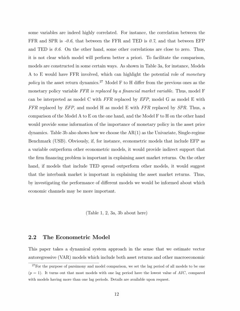
some variables are indeed highly correlated. For instance, the correlation between the

FFR and SPR is -0.6, that between the FFR and TED is 0.7, and that between EFP

and TED is 0.6. On the other hand, some other correlations are close to zero. Thus,

it is not clear which model will perform better a priori. To facilitate the comparison,

models are constructed in some certain ways. As shown in Table 3a, for instance, Models

A to E would have FFR involved, which can highlight the potential role of monetary

policy in the asset return dynamics.27 Model F to H differ from the previous ones as the

monetary policy variable FFR is replaced by a financial market variable. Thus, model F

can be interpreted as model C with FFR replaced by EFP, model G as model E with

FFR replaced by EFP, and model H as model E with FFR replaced by SPR. Thus, a

comparison of the Model A to E on the one hand, and the Model F to H on the other hand

would provide some information of the importance of monetary policy in the asset price

dynamics. Table 3b also shows how we choose the AR(1) as the Univariate, Single-regime

Benchmark (USB). Obviously, if, for instance, econometric models that include EFP as

a variable outperform other econometric models, it would provide indirect support that

the firm financing problem is important in explaining asset market returns. On the other

hand, if models that include TED spread outperform other models, it would suggest

that the interbank market is important in explaining the asset market returns. Thus,

by investigating the performance of different models we would be informed about which

economic channels may be more important.

(Table 1, 2, 3a, 3b about here)

2.2 The Econometric Model

This paper takes a dynamical system approach in the sense that we estimate vector

autoregressive (VAR) models which include both asset returns and other macroeconomic

27For the purpose of parsimony and model comparison, we set the lag period of all models to be one

( = 1). It turns out that most models with one lag period have the lowest value of , compared

with models having more than one lag periods. Details are available upon request.

12

and financial variables and allow them to interact with one another. Some justifications

have been discussed and we simply re-organize them here. First, much of the literature

takes a univariate approach and hence this paper, which takes an alternative approach, is

complementary. Second, it is well-known that when the regressors are not distinguishable

from integrated processes, the conclusions about return predictability could be altered.28

Under the VAR approach, this issue would become less severe because it is less likely that

the whole vector follows a unit root process than in the case of an individual variable. And

as we argued in the introduction, the reduced form dynamics of some dynamic, stochastic

general equilibrium models (DSGE) actually have a VAR representation. Hence, testing

the ability of a class of VAR models may provide an indirect test for a class of DSGE

models. Thus, the results in this paper could offer some hints for the future development

of DSGE models. In addition, while some of the existing literature tends to take one

of the returns as given and to use its movement to explain the other return, the VAR

approach naturally allows for dynamic interactions between the asset returns (housing

and stock) and other variables, as well as the feedback effects among asset returns. In

other words, it avoids assigning one of the asset returns as an “exogenous variable”, which

could lead to potential endogeneity bias.29

Our econometric model is a regime-switching VAR, with lag length for a (vector)

process :

0 () = () +

X=1

() − + () (1)

where we allow for all parameters, including intercept coefficients, autoregressive coeffi-

cients, and covariance matrix of stochastic terms to be contingent on the unobservable

state variable ∈ . The regime-dependent coefficients capture possible nonlinearities

or time variation in the lag structure of the model. The stochastic volatility allows for

possible heteroskedasticity of the stochastic terms.

The variables of interest = (1 2 )0 is a × 1 vector. The stochastic

intercept term () = (1 () 2 () ())0captures the difference in the intercept

28Among others, see Torous et al (2004), Cochrane (2008).29Among others, see Sims (1980a, b) for more discussion on these issues and the potential biases that

could be eliminated by the VAR method.

13

under different states. 0 () is a × state-dependent matrix that measures the

contemporaneous relationship between variables, and the econometric identification of

the model is obtained through restrictions on 0 (). In addition, () is a ×

matrix with each element state-dependent ()

(), = 1 = 1 . The

stochastic error term will be explained below.

The corresponding reduced form of the above model can be obtained by pre-multiplying (1)

by −10 (), which yields:

= () +

X=1

Φ () − + () (2)

where () = −10 () (), Φ () = −10 () (), and () = −10 () (),

= 1 2 . Φ () is a × matrix with each element which is state-dependent

()

(), = 1 = 1 . We further define

() ≡ + ()

which will be explained below. The vector of stochastic error term can be further

expressed as

= −10 () = Λ ()12 ()

where is a × diagonal matrix with diagonal elements 2 , = 1 , Λ () is a

× diagonal matrix with diagonal elements (), = 1 ,

Λ () =

⎡⎢⎢⎢⎢⎢⎣1 () 0 · · · 0

0 2 () · · · 0...

.... . .

...

0 0 · · · ()

⎤⎥⎥⎥⎥⎥⎦

which captures the difference in the intensity of volatility, and () is a vector of stan-

dard normal distribution, () ∼ (0Σ ()), where the covariance matrix is given

by

Σ () =

⎡⎢⎢⎢⎢⎢⎣1 21 () · · · 1 ()

12 () 1 · · · 2 ()...

.... . .

...

1 () 2 () · · · 1

⎤⎥⎥⎥⎥⎥⎦ (3)

14

We also include an “atheoretical benchmark,” which is the AR(), i.e. an order- auto-

regressive process that is labelled as the Univariate, Single-regime Benchmark (USB).

This is clearly motivated by the “efficient market hypothesis,” which conjectures that

all “relevant information” has been reflected in current (and potentially previous) period

price whereby additional variables, such as those provided by the VAR, are considered

insignificant. This could be the case of the stock return. On the other hand, the housing

market is always being accused of not being as efficient as the stock market, and hence the

housing market prediction can be improved with additional variables, including the stock

return. Hence, a comparison of model performance with USB provides not only a form

of “efficient market test,” but also an indirect test of the “cross-market informational

spillover.”30 For the linear VAR model, we include all 7 variables. For the regime-

switching models, we can only afford to include 4 variables, which is a much shorter

list than the linear model, as we need to estimate parameters in each regime, plus the

transition probabilities. By design, it puts regime-switching models in a disadvantageous

position. If, however, the regime-switching models still outperform the widely used linear

model, then it suggests that regime changes may indeed be very important in the data.

In addition, if models with certain variable(s) consistently outperform alternatives, then

such variable(s) may be important to account for in the asset return movements. Thus,

it may be important to include different combinations of our listed variables in different

models and test for the performance of those models.

For the linear VAR model, we include all 7 variables. For the regime switching

models, we can only afford to include 4 variables, which is a much shorter list than

the linear model, as we need to estimate parameters in each regime, plus the transition

probabilities. By design, this puts regime switching models in a disadvantageous position.

If, however, the regime switching models still outperform the widely used linear model,

then it suggests that regime changes may indeed be very important in the data. In

addition, if models with certain variable(s) consistently outperform alternatives, then

such variable(s) may be important to account for in the asset return movements. Thus,

it may be important to include different combinations of our listed variables in different

30Even for the case of aggregate output, it may still be a good idea to use an uni-variate AR(p) as the

benchmark. Among others, see Chauvet and Potter (2012) for more discussion.

15

models and test for the performance of those models.

2.3 Two-state Markov Process

Being severely constrained by the sample size, we assume that there are only two states,

i.e., ∈ = 1 2. The procedure for the identification of the regime of the economyfor a given period will be discussed below. The Markov switching process relates the

probability that regime prevails in to the prevailing regime in − 1, ( = |−1 = ) = . The transition probabilities are assumed to be constant and the transition

matrix is given by:31

=

⎛⎝ 11 1− 22

1− 11 22

⎞⎠

Given that the economy can be either in state 1 or state 2, the term () =

1 , defined above, captures the difference in the intercept under different states. For

convenience, we set (1) = 0 for = 1, thus (2) measures the difference in the

intercept between state 2 and state 1. Furthermore, we set the diagonal element of Λ ()

at state 1 to be unity, i.e., (1) = 1 so that if (2) 1, then the intensity of volatility

in state 2 is larger than that in state 1, and vice versa. Since () is a vector of standard

normal distribution and (1) is set to be one, the variance of = 1 , at state

1 is 2 , and the variance is 2 (2)

2 .

2.4 Identification of Regimes

Since the state of the economy is unobservable, we identify the regime for given a time

period by Hamilton’s (1989, 1994) smoothed probability approach, in which the proba-

bility of being state at time is given by ( | Ω ), where Ω = 1 2 .The idea is that we identify the state of the economy from an ex post point of view, and

thus the full set of information is utilized. Notice that we only allow for two regimes

31In principle, we could allow the transition probabilities to depend on the observed variables. However,

the time series we have assess to are relatively short and hence we make compromise in the modelling

choice.

16

in this paper, i.e., ∈ = 1 2. Thus, if ( = | Ω ) 05, then we identify the

economy most likely to be in state , = 1 2.32

2.5 Forecasting

After we estimate all the above models, we use the calculated probabilities of regime

switching for evaluating the forecasting performances of house and stock prices across

various models, and then examine both in-sample and out-of-sample forecasting perfor-

mances. We divide the sample into in-sample period 19752−20054 and out-of-sampleperiod 20061 and after. In any econometric model assessment, the calculation of confi-

dence interval is important, because it provides a quantitative sense on whether the point

estimate of the coefficient and predicted path of variables are “off the mark.” Clearly,

there is a large body of literature on “predictive regression” in asset pricing which have

applied different techniques to construct the confidence intervals. Phillips (2014) shows

through an analytical method and simulations that some commonly used methods in that

literature may be misleading. In particular, Phillips presents that “the commonly used Q

test is biased towards accepting predictability and associated confidence intervals for the

regressor coefficient asymptotically have zero converge probability in the stationary case.”

In light of these potential shortfalls, we conduct out-of-sample forecasting (OSF) in two

different approaches. The first approach is the conventional conditional moment method.

Given the estimation window 19752−20054 and a forecasting horizon = 1 4, theestimated parameters are used to forecast house and stock prices -step ahead outside

the estimation window, using the smoothed transition probabilities. The -step ahead

forecasted value of + based on model and information at time , Ω, is given by

(+ | Ω) =

2X=1

[+ | + = Ω]× (+ = | Ω)

where is the index for the state, and ∈ . The estimation window is then updated

consecutively with one observation and the parameters are re-estimated. Again the -

step ahead forecasts of house and stock prices are computed outside the new estimation

32In addition, we follow Francq and Zakoian (2001) to use spectrual radius to determine the stationarity

of the regime-switching models. Due to the space limit, we report the results in the appendix. We find

that most models are stationary. Only Model B and C are marginally non-stationary.

17

window. The procedure is iterated until the final observation. The forecasts based on

this method is basically to compute the -step ahead conditional expectations of the

variable being predicted. Most existing (non-Bayesian) works follow this method.

The second approach is the simulation method. A merit of this approach is that

we effectively simulate a “confidence interval” (CI) for ourselves and hence do not need

employ other approximation technique to construct the CI. In a sense, we avoid the

critique of Phillips (2013). The idea is simple. We simulate the path of the forecasted

values by repeated drawings. The procedure is as follows.

• (Step 1) We estimate the model using the estimation window 19752−20054 andobtain the parameters, transition probabilities, and variance-covariance matrix. Given

the estimation results we compute the smoothed probabilities to identify the regime at

the period 20054.

• (Step 2) Given the regime at the period 20054, we simulate the path of -stepahead regimes by random drawing, = 1 4.33 Given this particular path of -step

ahead regimes, we can obtain the path of predicted values of ∈ from (2).

• (Step 3) We iterate step 1 and 2 for 50 001 times to obtain the median of the -step ahead forecasted values during 20061−20064 and their corresponding confidenceintervals.

• We then update the sample with four more quarterly observations and repeat Step1-3, including re-estimating the model, in order to simulate the path of predicted values

for the subsequent four quarters. This procedure is repeated till the end of our sample.

An advantage of the second approach over the first one is that this method takes full

account of the regime switching model by determining the path of future regimes using

random drawing, rather than simply taking expectations over transition probabilities.

Another advantage is that a confidence interval is naturally generated, which enhances

33For example, suppose the regime identified at the time 20055 is state 1, we use the transition

probabilities 11 and 12 to generate the state at the period 20061. Specifically, we draw a value

from a uniform distribution [0 1]. The state at 20061 is state 1 if ∈ (0 11), and is state 2 ifotherwise. Suppose we have identified the state at 20061 to be state 2, then we use the transition

probabilities 21 and 22 to generate the state at the period 20062. Therefore, we will be able to

simulate the path of -step ahead regimes.

18

the evaluation of different models’ forecasting performance. It should be noticed that the

regime-switching nature of the model implies that the future forecast is path-dependent

and hence the conventional way to construct confidence interval may not be valid.

To evaluate the performances of in-sample and out-of-sample forecasts, we follow the

literature to compute two widely-used loss function for ∈ , which are the square loss

function, ³+|

´=P³

+|

´2and the absolute loss function,

³+|

´=P¯

+|

¯,

where +| be the -step forecast error of model , +| ≡ + − (+ | Ω). For

future reference, when we employ the square loss function as criteria to select models,

we label it as “the square loss criterion” (SLC). Similarly, when we use the absolute loss

function as criteria to select models, we label it as “the absolute loss criterion” (ALC).

Clearly, the SLC tends to penalize “big mistakes” more than the ALC. As it will be

clear later, our main conclusions do not depend on which criteria is used. We will then

combine these results with our newly proposed model comparison procedure, which will

be explained in more details in the following section.

2.6 Multi-lateral Model Comparison Procedures

On top of computing the differences in the loss functions for each model on the prediction

of both assets (housing and stock), we need a statistical procedure to compare whether

those differences are significant. Before we explain our procedure, it would be helpful

to provide a quick review of the current practice. The existing literature of applied

works adopt the Diebold-Mariano test (henceforth DM test) and its variants to assess

the “relative performance” of two models in a bilateral manner.34 While Diebold and

Mariano (1995), Zivot (2004) provide the details, it is nevertheless instructive to outline

the test here, as our procedure is closely related to the DM test. In our notations, the

Diebold-Mariano (henceforth DM) test is based on the “loss differential” ,

= ¡1+|

¢− ¡2+|

¢

34Diebold and Mariano test has been widely used in the literature. Among others, see Mariano and

Preve (2011) for a review of the literature.

19

where () is some loss function. Clearly, if the two models have roughly the same

predictive power, the expectation of the loss differential will be zero, [] = 0 If, instead,

Model 1 predicts better (worse) Model 2, the expected value of the loss differential will

be negative (positive).35 In practice, is unlikely to be exactly zero. The question is

then how we can decide whether Model 1 is in fact “significantly better (or worse)” than

Model 2. One of the contributions of DM test is that it shows that some function of

follows the standard normal distribution. Hence, a test statistics can be constructed so

that we can make judgement on models scientifically.

In application, researchers may need to choose among many alternatives. Typically,

researchers need execute the DM test repeatedly, and therefore the issue of ordering

naturally arises. For instance, consider the case of three competing models, A, B and

C. One may compare A against B first, and then compare the “winner” with C. One

may also compare A against C first and then compare the winner with B. Do these two

slightly different ordering deliver the same final winner? Clearly, as the number of models

increase, the number of possible ordering increases significantly and the importance of

ordering in model comparison might matter.36 Hansen et al (2011) develop a procedure

named as “model confidence set” (MCS). The idea is that we start with one model

and put that in the MCS. One then applies the DM test to compare that model with an

alternative. If both have the same predictive power in the sense that the “loss differential”

is smaller than certain critical value, then both models will be kept in the MCS;

otherwise, only the one with high predictive power will stay in the MCS. We repeat the

procedure until we exhaust all the models we have. The models in the remaining MCS

35The DM statistics will depend which is an average value of for different period , and the

co-variance of and − = 1 2 3 As shown by Zivot (2004), other things being equal, if model

1 which consistently over-predict in some sub-period and then consistently under-predict in other sub-

period, it is more likely to get not only a lower value of in different period t, but also a higher value

of co-variance and − = 1 2 3 As a result, model 1 is would be classified as under-perform the

alternative model. See Zivot (2004) for more details.36In fact, the situation is analogous to the old Condorcet Paradox, in which the candidate who wins

in every pair-wise situation may not be the winner when all candidates can be selected in one time. In

the present context, it means that the order of which model compares with which model would actually

affect the final outcome. For more discussion, see Austen-Smith and Banks (2000), among others.

20

will therefore have the same predictive power, and by construction they are better than

the models that are not selected into the MCS. Hence, while we still compare models in

a bilateral manner, we can still compare any finite set of models.

Mariano and Preve (2012), on the other front, generalize the idea of the DM test

and compare several models simultaneously (MP test). The idea is simple. Consider the

situation with ( + 1) models. We then define the “j-th loss differential”

= ³

+|

´−

³+1

+|

´, = 1 2 ,

where () continues to denote some loss function. We collect these loss differential in a

vector, = , = 1 2 . We then take average of it,

≡ 1

X=1

Mariano and Preve (2012) prove that ¡−

¢0 ³bΩ´−1 ¡− ¢ −→ 2 (in distribution),

where is the mean of the distribution, bΩ is a consistent estimator of the population

variance-covariance matrix Ω and is the degree of freedom. Thus, MP test enables us

to test whether all models of concern have the same predictive power.

In this paper we differentiate competing theories of asset prices, which are represented

by different econometrics models. Therefore, it is natural to use the MP test rather than

the DM test. Moreover, we need to define a procedure which enable us to categorize the

models into different “equivalent classes,” each of them contains model with (statistically

speaking) the same predictive power. The procedure needs to be “robust” in the sense

that the final outcome (i.e. the ranking of different models) would not be affected by the

ordering of which models are being compared first. Our procedures are similar to Hansen

et al (2011) and here are the steps.

1. We consider models that make predictions on the same economic variable. We

first rank models according to a criterion, such as SLC. Without loss of generality,

we assume that according to the chosen criteria, the predictive performance of

Model 1 is better than that of Model 2, which in turn is better than of Model 3,

and so on.

21

2. We conduct the MP test, in which the null hypothesis is that all models have the

same predictive power. If the hypothesis is not rejected, then by definition, all N

models have the same predictive power on a particular variable according to the

chosen criteria.

3. If the null hypothesis is rejected, then we eliminate the model with the least predic-

tive power. It can be easily identified as the models have been ranked according to

the predictive power in Step (1). We then repeat Step (2) until the null hypothesis

of equal predictive power is accepted.

4. Assume that in Step (3), there are 1 models which are found to possess the equal

predictive power, 1 0. For future reference, they are referred to as Class 1

among the models. By construction, there are ( − 1) models which do not

have the same predictive power as the models in Class 1. We now repeat Step (1)

on these ( −1) models until the null of equal predictive power is not rejected.

Assume that there are 2 models, 2 0, in the final list and they are identified

as Class 2.

5. If = 1 +2, then the procedure stops. The set of models are divided into two

classes, and models within each class have the same predictive power. Every model

in Class 1 has higher predictive power than any model in Class 2.

6. Now we consider the case that 1 + 2. Again, by construction, there are

( −1−2) models which do not have the same predictive power as the models

in Class 1 or Class 2. We now repeat Step (1) on these ( − 1 − 2) models

until the null of equal predictive power is not rejected. Assume that there are 3

models, 3 0, in the final list, and they are identified as Class 3.

7. If = 1 +2 +3, the the procedure stops.

8. If not, we repeat Step (6) and construct Class 4.

9. We repeat Step (8) until all N models are categorized into different classes. If there

are totally class, then it must be that = 1 +2 + +

22

10. We repeat the whole process with a change in the model evaluation criteria, e.g.

SLC being replaced by ALC.

Several remarks are in order. First, by definition, , = 1 2 3. . . must be positive.

In other words, each “Equivalent Predictive Power Class” (EPPC) is non-empty. In

addition, since models are first ranked according to a given criteria, our elimination

procedure is easy to implement. Second, by construction, all models within the same

class have the same predictive power, and any model in Class will always have higher

predictive power than any model in Class , for any , such that . Third, it

is possible that for the same set of models, the ranking will vary as the criteria

changes (say, from SLC to ALC), and hence the model can be categorized differently.

In other words, the classification of EPPC is criteria-dependent. In case the same set

of models have predictions on several economic variables (for instance, stock return

and housing return in this paper), it is also possible that the ranking of models also

varies with the variable we would like to predict. In other words, EPPC is also variable-

dependent. Notice also that this procedure still employs conventional criteria such as

SLC and ALC, and hence it facilitates a comparison with the literature. On the other

hand, our procedure allows us to compare a large number of competing models on a “fair

ground.” As computers become increasingly powerful and data availability improves over

time, we believe that comparison among a large number of alternative models may be

inevitable and the procedure we propose here can facilitate such a comparison. As we

present our empirical results, these features will become clear.

3 Estimation Results

Limited by data availability, we keep the model as parsimonious as possible. The details

of the estimation results for the whole sampling period 1975Q2-2012Q1 are presented in

the appendix, and Table 4a provides a summary. In general, a model allowing for regime

switching attains a lower value of Akaike’s information criterion (AIC) and a higher log-

likelihood value. Among all these models, the regime switching model G (EFP, TED,

23

SRET, HRET) has the best goodness of fit, i.e., a significantly lower value of AIC than

other models, suggesting that the credit market frictions and asset returns are indeed

significantly inter-related.

(Table 4a about here)

For the Markov switching model, recall that we set the volatility at regime 1 (1) = 1,

thus the element (2) measures the relative volatility of regime 2 over regime 1. In the

appendix the figures show that the estimated values of relative volatility (2) are all

significantly less than one for = 1 and 2, which means that for both federal funds rate

and the spread the volatility in regime 2 is lower than in regime 1. On the other hand,

almost all of the 3 (2) and 4 (2) are insignificant, suggesting that for the quarterly

stock and housing returns there is no significant difference in volatility across regimes.

Thus, we identify two regimes for this monetary policy tool: a high volatility regime

(regime 1) and a low volatility regime (regime 2). Table 4b provides a summary of the

estimated transition probabilities. It is clear that regimes are highly persistent, regardless

the models. In particular, most models suggest 11 to be close to 080 and all models

suggest 22 to be higher than 093. They imply that the expected duration of regime 1 to

be around 1(1−08) = 50 quarters and that for regime 2 is not less than 1(1−093) =14 3 quarters.

(Table 4b about here)

Given the estimated parameters, transition probabilities, and variance-covariance ma-

trices, we estimate the classification of regimes under different models and report the

results in Table 5. Basically, these models show similar classifications of the regimes. For

those periods identified as regime 1, all models include the aftermath of the second oil

crises and P. Volcker being appointed as Chairman of the Federal Reserve.37 Interest-

ingly, when the TED spread (TED) is included in Model E, G and H, the regime 1 also

includes the stock market crash in the 1987, suggesting that TED picks up the volatility

in the credit market after the stock market crash. It is also interesting that under Model

37Among others, Goodfriend and King (2005), Goodfriend (2007) provides a summary of the history

of monetary policy during that period.

24

E, which is like Model D except that EFP is replaced by the TED spread, the changes in

regimes are much more frequent. In general, models that involve TED would experience

more regime switching, suggesting higher variability of the risk premium faced by finan-

cial intermediations. We also compute the smoothed probabilities for all from Model B

to Model H, as shown in Figure 2. It shows the probabilities of the economy being in

regime 1 (high volatility regime) at a given period. Since there are only 2 regimes, the

probabilities of being in regime 2 would be suppressed.

(Table 5, Figure 2 about here)

4 Forecasting

We now proceed to forecast stock and housing returns. As discussed above we first

conduct in-sample forecasting for the period 1975Q2-2005Q4 and then examine the out-

of-sample forecasts for the period 2006Q1-2011Q4, using respectively the expectations-

based and simulation-based methods.

4.1 In-Sample Forecasting

We compute the loss functions based on SLC and ALC of in-sample -step ahead fore-

casts, = 1 4, for each variable across all models. Several findings are in order. First,

as shown in table 6a, the in-sample forecasts of asset returns are mixed. For the stock

returns, the model C (FFR, SPR, SRET, HRET) has the best performance. For housing

return, however, it is the Model E (FFR, TED, SRET, HRET) that out-perform all

others. Notice that both models contain the monetary policy variable FFR. It is true for

whether we use SLC or ALC. On the other hand, it seems that the performances in pre-

dicting stock returns across models are similar. We therefore implement our multi-lateral

model comparison procedures and attempt to categorize models into different “equivalent

predictive power class” (EPPC).38 Table 6b confirms our intuition. Whether we use SLC

38As a robustness check, we also use the conventional Diebold-Mariano test bilaterally and obtain very

similar results. The details are in the appendix.

25

or ALC, we find that all models have the same predictive power in terms of explaining

the stock return during the in-sample period. In particular, no model has superior per-

formance than an AR(1) process, which is the USB. It is consistent with the notion that

the stock market is very efficient in reflecting all the relevant information that adding

other variables in the statistical model does not provide any extra predictive power.

(Tables 6a, 6b about here)

For housing return, the situation is very different. Several observations are in order.

First, whether we use SLC or ALC, model D, E, F, H have the same predictive power

and they are always in Group 1, meaning that they are at least as good as the other

models. Second, whether we use SLC or ALC, model B (FFR, GDP, SRET, HRET)

and USB are always in the lowest group. This suggests that using the monetary policy

(FFR) and economic growth rate alone are not sufficient in understanding the housing

market, at least for the in-sample period (1975Q2-2005Q4). Alternatively, we may say

that the information in monetary policy and economic growth has been reflected in the

housing return itself. The fact that AR(1) (which is also USB for the housing return)

is always inferior to the four “good models” (Model D, E, F, H) suggests that there are

important information in the financial market that enhances our ability to account for the

housing market. Notice however that such “cross-market informational spillover” is very

subtle. Table 6c also shows that Model G (EFP, TED, SRET, HRET) is always inferior

to the four good models (Model D, E, F, H). However, Table 3 shows that Model F is

simply Model G with TED spread replaced by the term spread (SPR), and Model H is

simply Model G with the external finance premium (EFP) replaced by the term spread

(SPR). Does it mean that the term spread is so crucial in understanding the housing

return during that period? It does not seem to be the case, as both Model D and E,

which have the same predictive power as model F and H, do not contain SPR. Notice

that financial variables are correlated and hence some other variables may also contain

the information that is relevant in predicting future housing returns. To summarize, our

estimations indicate that the fact that the “efficient market hypothesis” does not apply

to the housing market during the in-sample period (1975 to 2005). The data are more

26

consistent with models which emphasize on imperfect capital market, such as Christiano,

Motto and Rostagno (2007), Davis (2010), Jin et al. (2012), among others.

4.2 Out-of-Sample Forecasting via Conditional-Expectation Es-

timation

We now turn to the out-of-sample forecasting (OSF) of housing and stock returns be-

ginning 20061, at the time when the growth of housing returns began to decline and

the sub-prime crisis started to unfold. Following the literature, we first conduct OSF

by using the conditional-expectations predictions. The appendix provides details of the

out-of-sample -step ahead forecasts, = 1 4, for each variable across all models.

Tables 6c summarize the results. In terms of forecasting stock returns, Model H (SPR,

TED, SRET, HRET) performs better than other models, both in terms of SLC and

ALC. In terms of forecasting housing returns, Model D (FFR, EFP, SRET, HRET) per-

forms better than other models, also both in terms of SLC and ALC. Naturally we ask

whether the difference is statistically significant. Again, we adopt the same procedure

and categorize models into different “equivalent predictive power class” (EPPC). Table

6d reports the results, and several observations are in order. In terms of stock return

forecasting, we find that (1) Model B, E, H and USB are always in Group 1, which means

that they are at least as good as other models, and (2) Model D and F are always in the

lower group. This is true whether we use SLC or ALC. The ranking of Model A, C, and

G will depend on which criteria is used, implying that there are models (especially D

an F) which under-perform the USB, which is the simple AR(1), in the out-of-sampling

forecasting of the stock return. Recall that for the in-sample forecasting, using the same

set of procedures and same set of models, we have found that all models have the same

predictive power. In other words, some models have actually deteriorated relative to the

USB (i.e. AR(1)) in terms of the ability of predicting the stock return. Notice that

both model D and F involve EFP, it may suggest that the ability of EFP to track the

aggregate stock return after the crisis is not as good as before.

(Tables 6c, 6d about here)

27

The case of OSF for the housing return is perhaps equally interesting. Table 6d clearly

shows that whether we use SLC or ALC, (1) Model C, D, F, G, H and USB are always

in Group 1, meaning that they have better predictive power, and (2), Model A, B, E are

always in Group 2, meaning that their predictive powers are not as good. Notice that

for in-sample forecasting, whether we use SLC or ALC, Model B (FFR, GDP, SRET,

HRET) and USB are always in the lowest group. For the out-of-sample forecasting,

Model B remains in the lowest group, yet the USB is “promoted” to the higher group. It

means that whether for the linear VAR with 7 variables (Model A), or regime-switching

VAR, no model in our list can out-perform the simple USB in terms of out-of-sample

forecasting of the housing return. Similar to the case of stock return forecasting, this

suggests that some models have deteriorated in terms of forecasting the housing return,

at least relative to the simple AR(1) process. In particular, model A and B are the only

models that involve GDP and yet they are always in group 2, suggesting that GDP may

not be as useful in predicting the house price as before. Clearly, the model comparison

here are far from conclusive and future research can revisit the issue with more rigorous

tools.

Another interesting observation is that, perhaps the forecasting ability of a model has

become more asset-specific for the out-of-sample forecast.39 For instance, while model

D and F are always the inferior models for stock return out-of-sample forecasting, they

are always in the Group 1 for the housing return forecasting. Similarly, while Model B

and E are always the “better” models in terms of out-of-sample forecast for the stock

return, they are always the “not-as-good” models in terms of out-of-sample forecast

for the housing return. Future research may investigate further on this phenomenon of

asset-dependent forecasting performance.

39Interestingly, this is also the case for structural models comparison. See Kwan et al. (2015), among

others, for more details.

28

4.3 Out-of-Sample Forecasting via Simulation

The results presented in the current section differ in at least two important dimensions

from the results presented in the previous section. First, the previous sections provide

only information of the “relative performance” of different models, as we use different sta-

tistical tools and procedures to assess whether some models have more superior predictive

power than the others. In this section, we attempt to assess the “absolute performance”

of different models by using simulation-based forecasting. Second, we aggregate the fore-

casting performance of each models during the whole out-of-sample period (2006 and

after) into some statistics and then compare across models in the previous section. In

the current section, we will compare the forecasting performance of different periods in

each year, and then allow the model to be re-estimated with updated data, and then

compare again in the subsequent year. Thus, we allow models to “learn and improve”

and would like to see which model(s) are more successful in adjust the parameter with

new data and hence provide more accurate forecasting over time.

We more specifically consider a forecasting window of 4 quarters starting 20061,

with -quarter ahead forecasts, = 1 4. After simulating the out-of-sample path

20061− 20064 based on observations up to 20054, the data are updated with fourobservations and the parameters are re-estimated. The procedure is repeated until we

have updated the sample to include all observations from 1975 to 2010 to predict the

asset returns in 2011. The purpose of this exercise is to see how the performances of the

models change when information is updated. The simulated paths together with their

80-percent confidence intervals can be visualized in Figure 3 for stock returns and Figure

4 for housing returns. Table 7a and 7b provide a summary of the performance of different

models

(Figure 3 and 4, Table 7a, 7b about here)

As shown in Figure 3a and 3b, the actual stock return and the predicted paths by

different models are well within the boundaries of the 80% confidence intervals for all five

models. Thus, although the models do not predict what have actually happened in 2006

and 2007, the models’ predictions are not that “far off the mark.” Unfortunately, with the

29

collapse of the Lehman Brothers, virtually all models are disappointing in the prediction

of 2008 returns (Figure 3c). Among them, Model G (EFP, TED, SRET, HRET) performs

worst in the sense that its 80-percent confidence interval does not even contain any of the

actual quarterly return in 2008. As we include the data up to 20084 and re-estimate

the models, the prediction of 2009 by models significantly improve. As shown by Figure

3d, each model’s confidence interval contains at least one quarter of stock return within

the confidence interval. Among them, Model D (FFR, EFP, SRET, HRET), Model E

(FFR, TED, SRET, HRET), Model F (EFP, SPR, SRET, HRET) and Model G contain

almost the path of the whole year stock return. With the data of 2009 included and

model updated, the prediction of 2010 is even better. As Figure 3e shows, each model’s

confidence interval contains at least one quarter of stock return. Interestingly, Model G,

which has the worst performance in 2008, becomes the best model of 2010 in the sense

that it is the only model whose confidence interval contains the whole path of quarterly

return of the year. The prediction of 2011 is similar. As Figure 3f shows, virtually all

models contain most of the year return, and all models unfortunately “miss” the drop

of stock return in 20113, as no model is able to generate a confidence interval which

contains the stock return in 20113.

As shown in Table 7b and Figure 4, the prediction of housing returns is worse than

the stock counterpart. Figure 4a shows that every models generates a confidence interval

that contains the path of the quarterly housing return of 2006yet as early as 2007, Figure

4b shows that the confidence intervals generated by our models fail to contain at least one

quarter of housing return. It should be notice that the same set of models successfully

contain the whole year path of stock return of the same year (2007). With 2007 data

included and model updated, the failure of 2008 is in a sense unexpected. Both Table

7b and Figure 4c show that the confidence intervals generated by more than half of our

models - namely, Model A (linear VAR with all 7 variables), Model B (FFR, GDP, SRET,

HRET), Model D (FFR, EFP, SRET, HRET), Model E (FFR, TED, SRET, HRET),

Model G (EFP, TED, SRET, HRET) - fail to contain any quarterly housing return in

2008. The remaining 4 models all miss at least one quarterly return of housing of the

year. Thus, while our models do not perform well in 2008 in predicting the stock return,

30

the prediction of housing return in the same year is much worse. With the information of

2008 included and model updated again, the prediction of 2009 is improved but perhaps

still disappointing. Recall that for the year 2009, the confidence interval generated by all

our models all contain some quarterly return of stock, suggesting that the enlargement

of the sample with model updating might improve the stock return forecasting. In the

case of housing, Figure 4d shows that Model B continues to fail to contain any quarterly

return of housing in 2009. While Model A, D, E, G make some improvements, the

confidence interval generated by the Model F (EFP, SPR, SRET, HRET) fail to contain

any quarterly housing return. And if the year 2008 and 2009 are disappointing year of

housing return forecasting, the year 2010 is a year with positive surprises. As shown

by Table 7b and Figure 4e show that all models successfully contain some quarterly

return of housing. Moreover, Model C (FFR, SPR, SRET, HRET), D, E and G are

able to generate confidence intervals that contain the whole year housing return. For

the case of stock return, only Model G contains the whole year of stock return in the

confidence interval. In this sense, the prediction of housing returns in 2010 is a success.

Unfortunately, Figure 4f shows that all models fail to contain the drop in housing return

in 20111, although they contain at least some quarterly return in the later part of the

same year. It is comparable to the performance of stock return prediction of the same

year (2011).

In sum, it seems that the OSF of asset returns is particularly difficult during this

period. In the case of stock return, Table 7a suggest that since 2008, most models will

miss at least one quarter of stock return, and while Model G “fails” in 2008, it becomes

very successful in 2010. This confirms the intuition that regularly incorporating new data

and re-estimating the model lead to better forecasting. In the case of the housing return,

most of our models, namely, Model A, B, D, E, F, G all experience at least one “missing

year” on either 2008 or 2009, i.e. a year in which the confidence interval generated by

the model does not contain any quarterly return of the year. At the same time, when we

re-estimate the model with data up to the end of 2009, model C, D, E, G successfully

capture the year 2010. In this sense, model G (EFP, TED, SRET, HRET) seems to be

the “best learner” in the sense that while it made mistakes in the 2008 or 2009, when it is

31

re-estimated with the data up to the end of 2009, it successfully captures the movements

in both stock return and housing return in 2010. Notice that according to table 7a

and 7b, neither the USB for stock return nor the USB for the housing return enjoys a

“perfect” year (i.e. the whole year asset return movement within the 80% confidence

interval) since 2006, suggesting that while the USB may be classified in the same EPPC

as other models during the out-of-sample period (2006 and after) as a whole, it may not

“learn” as much and as fast as other models which incorporate other macroeconomic and

financial variables.

4.4 Some Robustness Checks

Thus far, our analysis is based on using the data from 1975 to 2005 as in-sample, and

the periods after as out-of-sample, and then we progressively update the in-sample. As

a robustness check, we also re-estimate our models when we use the period from 1975

to 2006 as in-sample. Table 8 provides a summary and the details can be found in the

appendix. Notice that Table 8 is constructed analogous to Table 6 in order to facilitate

comparison. A few observations are in order. Table 8a shows that the best in-sample

forecasting performance comes from model C (FFR, SPR, SRET, HRET) for stock and

model E (FFR, TED, SRET, HRET) for housing, which is the same as the results in

Table 6a. While the details of the model classifications in Table 8b slightly differ from

Table 6b, some principal findings sustain. First, most, if not all, models are equally good

in predicting stock return during the in-sample period. Second, in terms of predicting

housing return, model B (FFR, GDP, SRET, HRET) and the USB are often the worst.

Again, this supports the idea that GDP is not very helpful even for in-sample prediction

of the housing return, and information about the future housing returns are reflected

in economic variables other than the current housing return. Table 8c shows that the

principal result of Table 6c also sustains, namely, model H (SPR, TED, SRET, HRET)

out-performs other models in terms of out-of-sample forecasting of stock returns, and

model D (FFR, EFP, SRET, HRET) out-performs other models in terms of out-of-

sample forecasting of housing returns. Table 8d, which provides the model classification

32

in terms of out-of-sample forecasts is also similar to Table 6d. More specifically, the

model classification in terms of out-of-sample 4-quarter ahead forecasts of stock return

are identical. In terms of the counterpart of housing returns forecast, model A (linear

VAR with all 7 variables), model B which contains FFR and GDP and model E which

contains FFR and TED are inferior to models C, D, F, G. A noticeable difference is that

now model H which contains SPR and TED, and USB are also in the second class. Thus,

it seems that while the choice of choosing 2005 as the end of the in-sample might not be

the consensus among researchers, the results are not as sensitive as one may think. In

addition, the previous section has also presented our results based on a recursive approach

of allowing models to “update and re-estimate” in terms of the out-of-sample forecasting.

(Tables 8a, 8b, 8c, 8d about here)

5 Concluding Remarks

Dramatic movements in asset prices often occupy media headlines and carry implications

in real economic activities, even political personnel changes. Yet in media and even aca-

demic circles are full of competing and sometimes even conflicting explanations. This

paper attempts to bring some explanations for these events to formal testing. Notice

that while an econometric model comparison is not equivalent to an explanation compar-

ison, the exercise in this paper may provide us hints for future model development. It is

especially true if models contain certain variables consistently out-perform other models

which do not contain those variables. From a policy point of view, identifying the em-

pirically more relevant model does not only satisfies intellectual curiosity, but may also

assist governments making more appropriate policy decisions. Thus, this paper attempts

to establish some stylized facts about the asset return dynamics in the aggregate level. In

particular, this paper separates the data into the pre-crisis period 1975-2005 (in-sample)

and the period after (2006-2011), and examines whether an estimated model based on

the pre-crisis period can have reasonable forecasting for the crisis period (out-of-sample

33

forecasting), with the effect of other variables such as GDP growth and monetary policy

taken into consideration.

Our first contribution is to demonstrate how to categorize competing models into dif-

ferent “Equivalence Predictive Power Classes” (EPPC). We find that it can shed light on

the Efficient Market Hypothesis (EMH) debate, as well as the structural-break discussion

on the asset markets. During the in-sample period, all models have the same predictive

power as the USB (Univariate, Single-regime Benchmark, i.e. AR()) on stock return.

It is consistent with the EMH that all information about the future stock returns has

been reflected in the current period stock return and hence additional variables do not

enhance the forecasting. For the housing return, the situation is different. Model D, E,

F, H consistently outperform the USB, suggest the existence of cross-market information

flow and the value of multi-variate modeling. For the out-of-sample period as a whole,

the picture changes. No model has superior predictive power than the USB on either

the stock return of housing return forecast. Whether we use the “square loss criterion”

(SLC) or the “absolute loss criterion” (ALC), and Model A, B and E are shown to have

lower predictive power than the USB in the housing return forecast. Thus, these results

seem to be consistent with the notion that there are some “structural changes” in the

determinants of asset return dynamics since 2006. In particular, since both Model A

and B are the only models which contain GDP as a variable in the dynamical system,

the evidence then points to the possibility that GDP has lost its power in predicting the

housing return after the crisis period, perhaps due to the deep recession. Obviously, it

does not mean that “economic fundamentals” such as GDP is not important. One inter-

pretation is that the information contained in the GDP has already been reflected in other

financial variables that we include in the econometric model, such as TED spread. This

is consistent with the theoretical result in Telmer and Zin (2002) that with incomplete

markets, asset returns can predict (future) asset prices well.

Our second contribution shows that all models do not have the same capacity to “learn

and update.” Notice that the results based on EPPC clearly treat the model performance

during the out-of-sample period as a whole. However, it is possible that some models

make more mistake in the beginning of the financial crisis, and later improves significantly

34

with new data is supplied. To investigate such possibility, we conduct out-of-sampling

forecasting based on the simulation approach. We find that the USB of either the stock

return or the housing return never enjoys a perfect year (i.e. a year that the asset return

is totally inclusive within the confidence interval) since 2006. On the other hand, after

revising with data by the end of 2009, Model G, which includes both the EFP and TED

spread, can include the actual asset returns of 2010 in the confidence intervals. In other

words, while uni-variate models may be as good as any model in predicting asset returns

in the “long run,” they may learn “slower” than multi-variate ones in the “short-run”. It

also suggests that macroeconomic models, which emphasize the role of imperfect capital

market faced by non-financial firms as well as those faced by banks, may be promising

in enhancing the understanding of the stock and housing returns.40

In addition,we also methodologically demonstrate a few things in terms of multi-

variate modeling. First, the widely used linear VAR model (i.e. single regime) with 7

variables can actually under-perform than the regime-switching counterparts with only

4 variables most of the time. Perhaps more importantly, we demonstrate that we can

combine the multi-model comparison test of Mariano and Preve (2012) with the “Model

Confidence set” procedure developed by Hansen et al. (2011) to classify models into

different EPPC. We also demonstrate that such EPPC approach can be complemented

by the simulation-based method used by Sargent, Williams and Zha (2006) and others to

further distinguish the empirical performance of models within the same EPPC. Future

research may want to further explore along these lines.

This research can clearly be extended in several dimensions. First, it would be in-

teresting to apply the current econometric framework to other economies, such as the

European Union countries. The current framework can also be applied to more disag-

gregate data. Also, it would be interesting to incorporate higher frequency variables and

study the (potential) price discovery processes among different asset markets. Needless

to say, one can re-examine the two asset markets with Bayesian econometrics. Finally,

one could develop a theoretical framework that mimics the stylized facts found in this

paper, which will further enhance our understanding of the interactions between the real

40Among others, see Gertler and Kiyotaki (2010), Davis (2010), Andres and Arce (2012), Jin et al.

(2012).

35

economy and the asset markets.

36

References

[1] Andres, J. and O. Arce, 2012, Banking competition, housing prices and macroeco-nomic stability, Economic Journal, 122, 1346-372.

[2] Austen-Smith, D. and J. Banks, 2000, Positive Political Theory I: Collective Pref-erence, Ann Arbor: University of Michigan Press.

[3] Bank for International Settlements, 2003, 73rd Annual Report, Basle.

[4] Bernanke, B. and M. Gertler,1995, Inside the black box: The credit channel ofmonetary policy transmission, Journal of Economic Perspectives 9, 27-48.

[5] Bernanke, B. and M. Gertler, 2001, Should central banks respond to movements inasset prices? American Economic Review, 91, 253-257.

[6] Bernanke, B., M. Gertler and S. Gilchrist, 1999, The Financial Accelerator in AQuantitative Business Cycle Framework, in John Taylor and Michael Woodford(ed.), Handbook of Macroeconomics, Vol. 1, New York: Elsevier.

[7] Bertay, A. C. and D. Gong, 2014, Securitization, financial stability and macroecon-omy: Evidence from an international panel, mimeo.

[8] Campbell, J. Y. and J. F. Cocco, 2007, How do house prices affect consumption?Evidence from micro data, Journal of Monetary Economics, 54, 591-621.

[9] Case, K. E. and R. J. Shiller, 1990, Forecasting prices and excess returns in thehousing market, Real Estate Economics, 18, 253-73.

[10] Case, K. E., J. Quigley and R. J. Shiller, 2005, Comparing wealth effects: the stockmarket versus the housing market, Advances in Macroeconomics, 5, 1235-1235.

[11] Cetorelli, N. and L. Goldberg, 2011, Global banks and international shock transmis-sion: Evidence from the crisis, IMF Economic Review, 59, 41-76.

[12] Cetorelli, N. and L. Goldberg, 2012, Banking globalization and monetary transmis-sion, Journal of Finance, 67, 1811-1843.

[13] Chang, K. L., N. K. Chen and C. K. Y. Leung, 2011, Monetary policy, term structureand real estate return: Comparing REIT, housing and stock, Journal of Real EstateFinance and Economics, 43, 221-257.

[14] Chang, K. L., N. K. Chen and C. K. Y. Leung, 2012, The dynamics of housing re-turns in Singapore: How important are the international transmission mechanisms?Regional Science and Urban Economics, 42, 516-530.

[15] Chang, K. L., N. K. Chen and C. K. Y. Leung, 2013, In the shadow of the UnitedStates: The international transmission effect of asset returns, Pacific Economic Re-view, 18(1), 1-40.

[16] Chauvet, M. and S. Potter, 2013, Forecasting output, G. Elliot and A. Timmenmannet., Handbook of Economic Forecasting, volume 2, part A, 141-194.

37

[17] Chen, N. K., H. L. Cheng and C. S. Mao, 2014, Identifying and forecasting houseprices: A macroeconomic perspective, Quantitative Finance, 14, 2105-2120.

[18] Chen, N. K. and C. K. Y. Leung, 2008, Asset price spillover, collateral and crises:With an application to property market policy, Journal of Real Estate Finance andEconomics, 37, 351-385.

[19] Christiano, L., R. Motto and M. Rostagno, 2007, Financial factors in business cycles,Northwestern University, mimeo.

[20] Clapp, J. M. and C. Giaccotto, 1994, The influence of economic variables on localhouse price dynamics, Journal of Urban Economics 36, 161-83.

[21] Clark, T., 2011, Real-time density forecasts from Bayesian vector autoregressionswith stochastic volatility, Journal of Business and Economic Statistics, 29, 327-341.

[22] Cochrane, J., 2001, Asset Pricing, Princeton: Princeton University Press.

[23] Cooley, T. and M. Dwyer, 1998. Business cycle analysis without much theory: Alook at structural VARs. Journal of Econometrics, 83(1-2), 57-88.

[24] Davis, S., 2010, The adverse feedback loop and the real effects of financial sectoruncertainty, Vanderbilt University, mimeo.

[25] De Walque, G., O. Pierrard and A. Rouabah, 2010, Financial (in)stability, super-vision and liquidity injections: A dynamic general equilibrium approach, EconomicJournal, 120(549), 1234-1261.

[26] Darrat, A. and J. Glascock, 1989, Real estate returns, money and fiscal deficits: Isthe real estate market efficient? Journal of Real Estate Finance and Economics, 2,197-208.

[27] Diebold, F. and R. Mariano, 1995, Comparing predictive accuracy, Journal of Busi-ness & Economic Statistics, 13, 253-263.

[28] Emiris, M., 2006, The term structure of interest rates in a DSGE model, NationalBank of Belgium, mimeo.

[29] Estrella, A., 2005, Why does the yield curve predict output and inflation? EconomicJournal, 115, 722-44.

[30] Estrella, A. and M. R. Trubin, 2006, The yield curve as a leading indicator: Somepractical issues, Current Issues in Economics and Finance 12, Federal Reserve Bankof New York.

[31] Fama, E., 1970, Efficient capital markets: A review of theory and empirical work,Journal of Finance, 25(2), 383-417.

[32] Ferreira, F., J. Gyourko and J. Tracy, 2010, Housing busts and household mobility,Journal of Urban Economics, 68(1), 34—45.

[33] Francq, C. and J. M. Zakoian, 2001, Stationary of multivariate Markov-switchingARMA models, Journal of Econometrics 10, 339-364.

[34] Gertler, M. and C. Lown, 1999, The information in the high-yield bond spread forthe business cycle: Evidence and some implications, Oxford Review of EconomicPolicy, 15, 132-150.

38

[35] Gertler, M. and N. Kiyotaki, 2010, Financial intermediation and credit policy inbusiness cycle analysis, in B. M. Friedman and M. Woodford ed., Handbook ofMonetary Economics, Vol. 3, 547-599.

[36] Goodhart, C., 2001, What weight should be given to asset prices in the measurementof inflation? Economic Journal 111, 335-356.

[37] Goodhart, C. and B. Hofmann, 2007, House Prices and the Macroeconomy: Impli-cations for Banking and Price Stability, Oxford: Oxford University Press.

[38] Green, R., 2002, Stock prices and house prices in California: New evidence of awealth effect? Regional Science and Urban Economics, 32, 775-783.

[39] De Graeve, F., 2007, The external finance premium and the macroeconomy: USPost-WWII evidence, working paper.

[40] Grishchenko, O. V. and M. Rossi, 2012, The role of heterogeneity in asset pricing:The effect of a clustering approach, Journal of Business and Economic Statistics, 30,297-311.

[41] Hamilton, J., 1994, Time series analysis, Princeton: Princeton University Press.

[42] Hansen, P., A. Lunde and J. Nason, 2011, The model confidence set, Econometrica,79(2), 453-497.

[43] Hempel, C. G., 1942, The function of general laws in history, Journal of Philosophy,39(2), 35-48.

[44] Himmelberg, C., C. Mayer and T. Sinai, 2005, Assessing high house prices: Bubbles,fundamentals and misperceptions, Journal of Economic Perspective, 19, 67-92.

[45] Hott, C. and P. Monnin, 2008, Fundamental real estate prices: An empirical esti-mation with international data, Journal of Real Estate Finance and Economics, 36,427-450.

[46] Huang, H., and Y. Tang, 2012, Residential land use regulation and the US housingprice cycle between 2000 and 2009, Journal of Urban Economics, 71(1), 93—99.

[47] Huang, M., 2014, Bubble-like housing boom—bust cycles: Evidence from the predic-tive power of households’ expectations, Quarterly Review of Economics and Finance,54, 2-16

[48] Ibbotson, R. G. and L. B. Siegel, 1984, Real estate returns: A comparison with otherinvestments, Journal of American Real Estate and Urban Economics Association,12, 219-242.

[49] In’t-Veld, J., R. Raciborski, M. Ratto and W. Roeger, 2011, The recent boom—bustcycle: The relative contribution of capital flows, credit supply and asset bubbles.European Economic Review, 55(3), 386—406.

[50] Jin, Y., C. K. Y. Leung and Z. Zeng 2012, Real estate, the external finance premiumand business investment: A quantitative dynamic general equilibrium analysis, RealEstate Economics, 40(1), 167-195.

[51] Kan, K., S. K. S. Kwong and C. K. Y. Leung, 2004, The dynamics and volatilityof commercial and residential property prices: Theory and evidence, Journal ofRegional Science, 44(1), 95-123.

39

[52] Kapetanios, G., A. Pagan and A. Scott, 2007, Making a match: Combining theoryand evidence in policy-oriented macroeconomic modeling, Journal of Econometrics,136, 565-594.

[53] Khandani, A. E., A. W. Lo and R. C. Merton, 2013, Systemic risk and the refinancingratchet effect, Journal of Financial Economics, 108(1), 29—45.

[54] King, R., C. Plosser and S. Rebelo, 2002, Production, growth and business cycles:Technical appendix, Computational Economics, 20, 87—116.

[55] Kiyotaki, N. and J. Moore, 1997, Credit cycles, Journal of Political Economy, 105,211-248.

[56] Kouwenberg, R. and R. Zwinkels, 2014, Forecasting the US housing market, Inter-national Journal of Forecasting, 30, 415-425.

[57] Kwan, Y. K., C. K.Y. Leung and J. Dong, 2015, Comparing consumption-basedasset pricing models: The case of an Asian city, Journal of Housing Economics, 28,18-41.

[58] LeRoy, S., 1989, Efficient capital markets and Martingales, Journal of EconomicLiterature, 27(4), 1583-1621.

[59] Lettau, M. and S. C. Ludvigson, 2005, Expected returns and expected dividendgrowth, Journal of Financial Economics,76, 583-626.

[60] Leung, C., 2004, Macroeconomics and housing: a review of the literature, Journalof Housing Economics, 13, 249-267.

[61] Leung, C. K. Y., 2007, Equilibrium correlations of asset price and return, Journalof Real Estate Finance and Economics, 34, 233-256.

[62] Leung, C. K. Y., 2014, Error correction dynamics of house pice: An equilibriumbenchmark, Journal of Housing Economics, 25, 75-95.

[63] Lubik, T., and F. Schorfheide, 2004, Testing for indeterminacy: An application toU.S. monetary policy, American Economic Review, 94(1), 190-217.

[64] Lustig, H. and S. Van Nieuwerburgh, 2005, Housing collateral, consumption insur-ance and risk premia: An empirical perspective, Journal of Finance, 60, 1167—1219.

[65] Lutz, B., R. Molloy, and H. Shan, 2011, The housing crisis and state and localgovernment tax revenue: Five channels. Regional Science and Urban Economics,41(4), 306—319.

[66] Maheu, J. and T. McCurdy, 2000, Identifying bull and bear markets in stock returns.Journal of Business and Economic Statistics 18, 100—112.

[67] Maheu, J., T. McCurdy, Y. Song, 2012, Components of Bull and Bear markets:Bull corrections and Bear rallies, Journal of Business and Economic Statistics 30,391-403.

[68] Mariano, R. and D. Preve, 2012, Statistical tests for multiple forecast comparison,Journal of Econometrics, 169, 123-130.

[69] Menzly, L., T. Santos and P. Veronesi, 2004, Understanding predictability, Journalof Political Economy, 112, 1-47.

40

[70] Mishkin, F., 2001, The transmission mechanism and the role of asset prices in mon-etary policy, NBER Working Paper 8617.

[71] Nichols, J. B., S. D. Oliner and M. R. Mulhall, 2013, Swings in commercial andresidential land prices in the United States. Journal of Urban Economics, 73(1),57-76.

[72] Pagan, A. and T. Robinson, Methods for assessing the impact of financial effects onbusiness cycles in macroeconometric models, Journal of Macroeconomics, 41, 94-106.

[73] Phillips, P., 2014, On confidence intervals for autoregressive roots and predictiveregression, Econometrica, 82(3), 1177-1195.

[74] Piazzesi, M., M. Schneider and S. Tuzel, 2007, Housing, consumption, and assetpricing, Journal of Financial Economics, 83, 531-569.

[75] Plosser, C. and K. G. Rouwenhorst, 1994, International term structures and realeconomic growth, Journal of Monetary Economics, 33, 133-155.

[76] Quan, D. and S. Titman, 1997. Commercial real estate prices and stock marketreturns: An international analysis, Financial Analysts Journal, 53(3), 21-34.

[77] Quan, D. and S. Titman, 1999. Do real estate prices and stock prices move together?An international analysis, Real Estate Economics, 27, 183-207.

[78] Rigobon, R. and B. Sack, 2003. Measuring the reaction of monetary policy to thestock market, Quarterly Journal of Economics, 118, 639—669.

[79] Rosenberg, J. V. and S. Maurer, 2008, Signal or noise? Implications of the termpremium for recession forecasting, FRBNY Economic Policy Review, 14(3), 1-11.

[80] Sargent, T., N. Williams and T. Zha, 2006, Shocks and government beliefs: The riseand fall of American inflation, American Economic Review, 96, 1193-1224.

[81] Shiller, R., 2007, Understanding recent trends in house prices and home owner-ship. Retrieved fromhttp://www.kc.frb.org/publicat/sympos/2007/pdf/2007.09.27.shiller.pdf.

[82] Shiller, R., 2008, The Subprime Solution, Princeton: Princeton University Press.

[83] Sims, C., 1980a, Comparison of interwar and postwar business cycles: Monetarismreconsidered, American Economic Review, 70(2), 250-257.

[84] Sims, C., 1980b, Macroeconomics and reality, Econometrica, 48, 1-48.

[85] Sims, C. and T. Zha, 2006, Were there regime switches in U.S. monetary policy?American Economic Review, 96, 54-81.

[86] Sutton, G. D., 2002, Explaining changes in house prices, BIS Quarterly Review,September, 46-55.

[87] Telmer, C. and S. Zin, 2002, Prices as factors: Approximate aggregation with in-complete markets, Journal of Economic Dynamics and Control, 26, 1127-1157.

[88] Torous, W., R. Valkanov and S. Yan, 2004, On predicting stock returns with nearlyintegrated explanatory variables, Journal of Business, 77, 937-966.

41

[89] Tsatsaronis, K. and H. Zhu, 2004, What dirves housing price dynamics: Cross-country evidence, BIS Quarterly Review, March, 65-78.

[90] Welch, I. and A. Goyal, 2008, A comprehensive look at the empirical performanceof equity premium prediction, Review of Financial Studies, 21(4), 1455-1508.

[91] Yoshida, J., 2008, Technology shocks and asset price dynamics: The role of housingin general equilibrium, University of Tokyo, mimeo.

[92] Zivot, E., 2004, Notes on forecasting, University of Washington at Seattle, mimeo.

42

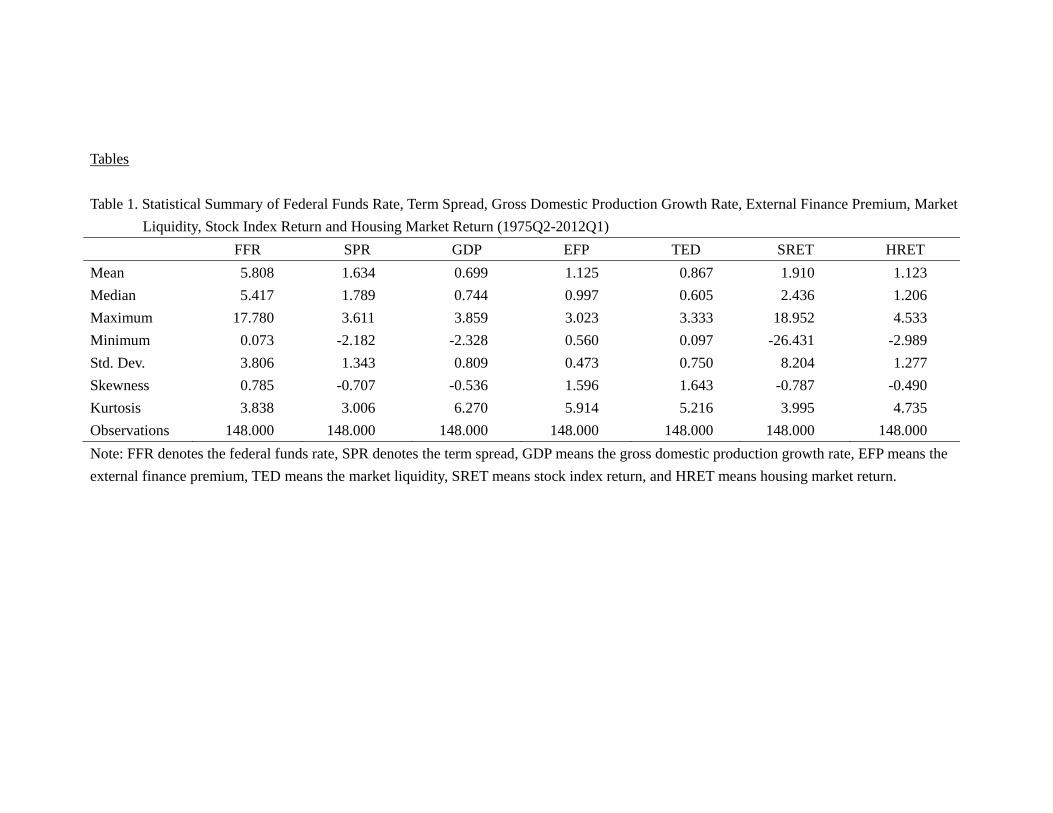
Tables Table 1. Statistical Summary of Federal Funds Rate, Term Spread, Gross Domestic Production Growth Rate, External Finance Premium, Market

Liquidity, Stock Index Return and Housing Market Return (1975Q2-2012Q1) FFR SPR GDP EFP TED SRET HRET Mean 5.808 1.634 0.699 1.125 0.867 1.910 1.123 Median 5.417 1.789 0.744 0.997 0.605 2.436 1.206 Maximum 17.780 3.611 3.859 3.023 3.333 18.952 4.533 Minimum 0.073 -2.182 -2.328 0.560 0.097 -26.431 -2.989 Std. Dev. 3.806 1.343 0.809 0.473 0.750 8.204 1.277 Skewness 0.785 -0.707 -0.536 1.596 1.643 -0.787 -0.490 Kurtosis 3.838 3.006 6.270 5.914 5.216 3.995 4.735 Observations 148.000 148.000 148.000 148.000 148.000 148.000 148.000 Note: FFR denotes the federal funds rate, SPR denotes the term spread, GDP means the gross domestic production growth rate, EFP means the external finance premium, TED means the market liquidity, SRET means stock index return, and HRET means housing market return.

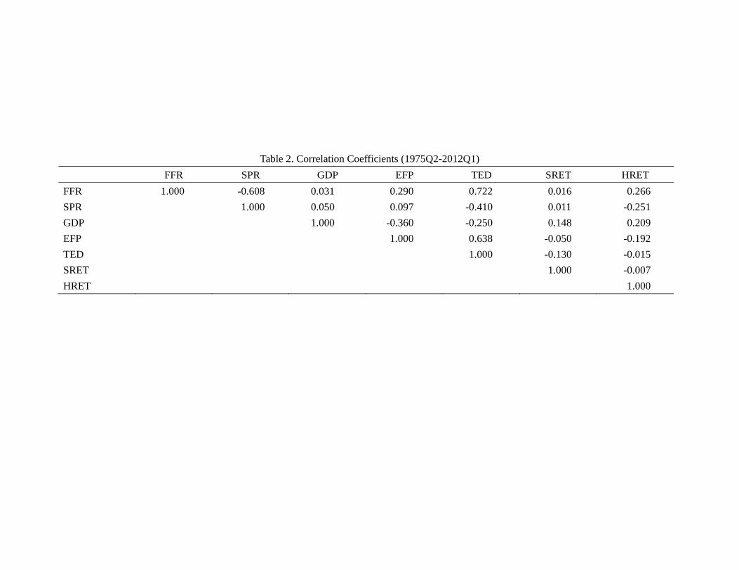
Table 2. Correlation Coefficients (1975Q2-2012Q1) FFR SPR GDP EFP TED SRET HRET FFR 1.000 -0.608 0.031 0.290 0.722 0.016 0.266 SPR 1.000 0.050 0.097 -0.410 0.011 -0.251 GDP 1.000 -0.360 -0.250 0.148 0.209 EFP 1.000 0.638 -0.050 -0.192 TED 1.000 -0.130 -0.015 SRET 1.000 -0.007 HRET 1.000

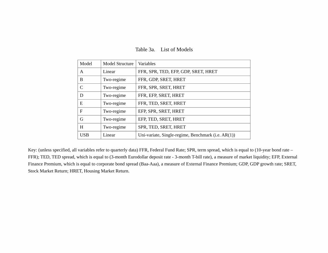
Table 3a. List of Models

Model Model Structure Variables

A Linear FFR, SPR, TED, EFP, GDP, SRET, HRET

B Two-regime FFR, GDP, SRET, HRET

C Two-regime FFR, SPR, SRET, HRET

D Two-regime FFR, EFP, SRET, HRET

E Two-regime FFR, TED, SRET, HRET

F Two-regime EFP, SPR, SRET, HRET

G Two-regime EFP, TED, SRET, HRET

H Two-regime SPR, TED, SRET, HRET

USB Linear Uni-variate, Single-regime, Benchmark (i.e. AR(1))

Key: (unless specified, all variables refer to quarterly data) FFR, Federal Fund Rate; SPR, term spread, which is equal to (10-year bond rate – FFR); TED, TED spread, which is equal to (3-month Eurodollar deposit rate - 3-month T-bill rate), a measure of market liquidity; EFP, External Finance Premium, which is equal to corporate bond spread (Baa-Aaa), a measure of External Finance Premium; GDP, GDP growth rate; SRET, Stock Market Return; HRET, Housing Market Return.

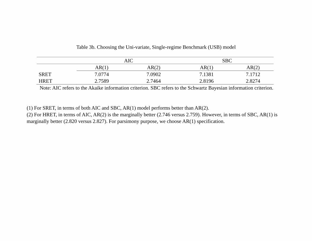
Table 3b. Choosing the Uni-variate, Single-regime Benchmark (USB) model

AIC SBC AR(1) AR(2) AR(1) AR(2) SRET 7.0774 7.0902 7.1381 7.1712 HRET 2.7589 2.7464 2.8196 2.8274 Note: AIC refers to the Akaike information criterion. SBC refers to the Schwartz Bayesian information criterion.

(1) For SRET, in terms of both AIC and SBC, AR(1) model performs better than AR(2). (2) For HRET, in terms of AIC, AR(2) is the marginally better (2.746 versus 2.759). However, in terms of SBC, AR(1) is marginally better (2.820 versus 2.827). For parsimony purpose, we choose AR(1) specification.

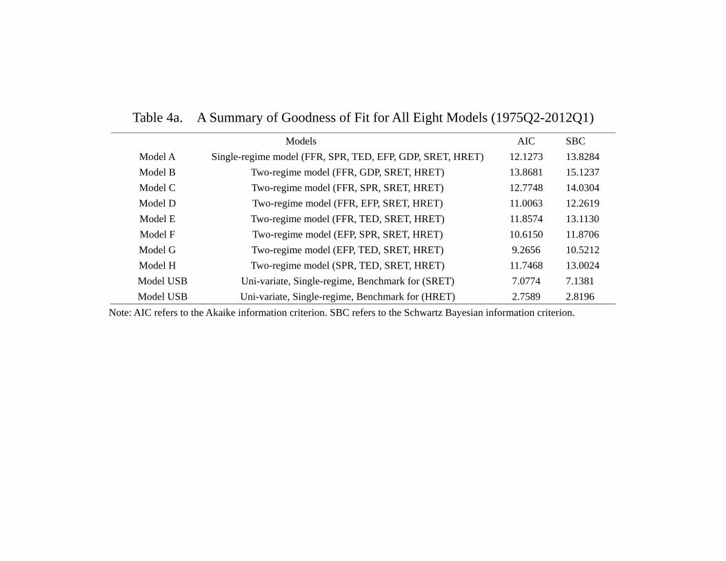
Table 4a. A Summary of Goodness of Fit for All Eight Models (1975Q2-2012Q1) Models AIC SBC

Model A Single-regime model (FFR, SPR, TED, EFP, GDP, SRET, HRET) 12.1273 13.8284 Model B Two-regime model (FFR, GDP, SRET, HRET) 13.8681 15.1237 Model C Two-regime model (FFR, SPR, SRET, HRET) 12.7748 14.0304 Model D Two-regime model (FFR, EFP, SRET, HRET) 11.0063 12.2619 Model E Two-regime model (FFR, TED, SRET, HRET) 11.8574 13.1130 Model F Two-regime model (EFP, SPR, SRET, HRET) 10.6150 11.8706 Model G Two-regime model (EFP, TED, SRET, HRET) 9.2656 10.5212 Model H Two-regime model (SPR, TED, SRET, HRET) 11.7468 13.0024

Model USB Uni-variate, Single-regime, Benchmark for (SRET) 7.0774 7.1381 Model USB Uni-variate, Single-regime, Benchmark for (HRET) 2.7589 2.8196

Note: AIC refers to the Akaike information criterion. SBC refers to the Schwartz Bayesian information criterion.

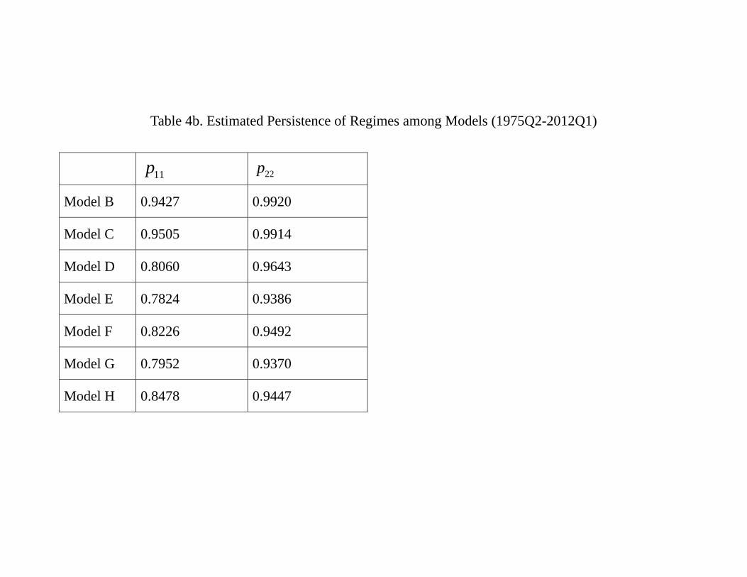
Table 4b. Estimated Persistence of Regimes among Models (1975Q2-2012Q1)

11p 22p

Model B 0.9427 0.9920

Model C 0.9505 0.9914

Model D 0.8060 0.9643

Model E 0.7824 0.9386

Model F 0.8226 0.9492

Model G 0.7952 0.9370

Model H 0.8478 0.9447

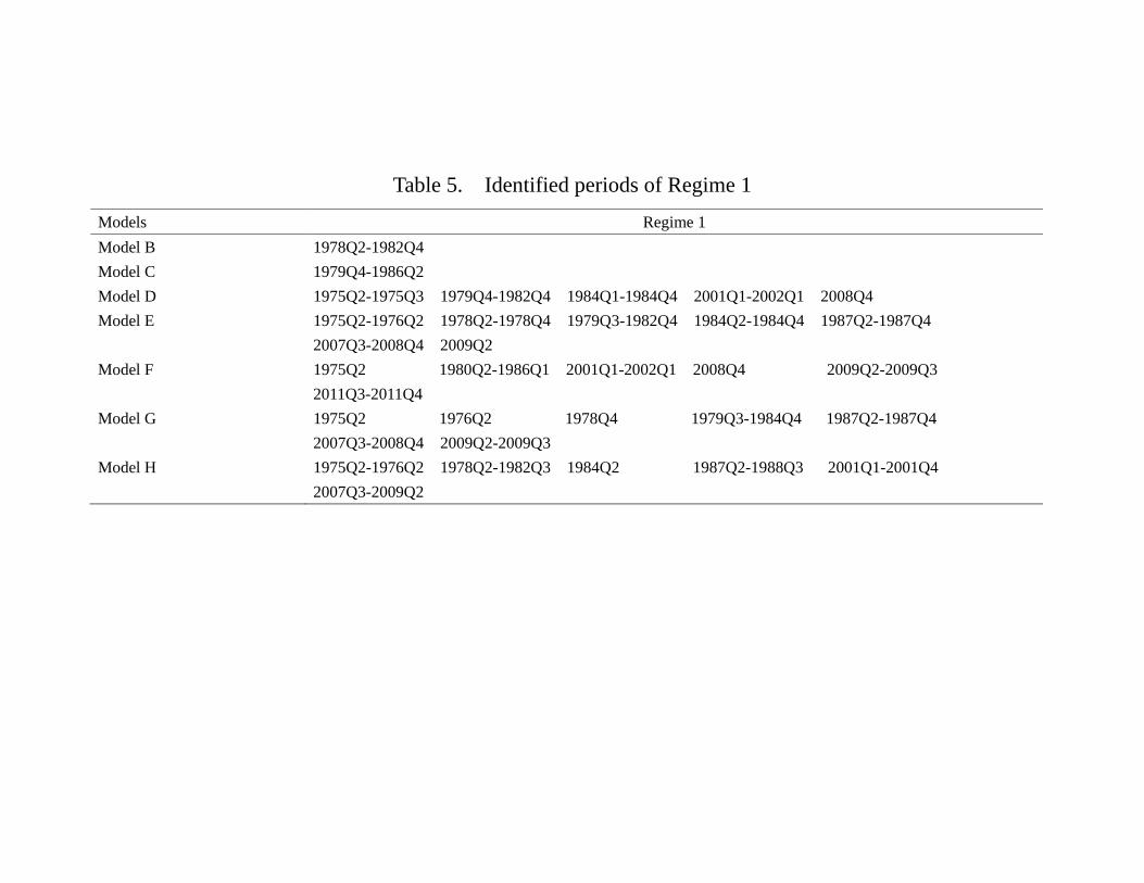
Table 5. Identified periods of Regime 1 Models Regime 1 Model B 1978Q2-1982Q4 Model C 1979Q4-1986Q2 Model D 1975Q2-1975Q3 1979Q4-1982Q4 1984Q1-1984Q4 2001Q1-2002Q1 2008Q4 Model E 1975Q2-1976Q2 1978Q2-1978Q4 1979Q3-1982Q4 1984Q2-1984Q4 1987Q2-1987Q4

2007Q3-2008Q4 2009Q2 Model F 1975Q2 1980Q2-1986Q1 2001Q1-2002Q1 2008Q4 2009Q2-2009Q3

2011Q3-2011Q4 Model G 1975Q2 1976Q2 1978Q4 1979Q3-1984Q4 1987Q2-1987Q4

2007Q3-2008Q4 2009Q2-2009Q3 Model H 1975Q2-1976Q2 1978Q2-1982Q3 1984Q2 1987Q2-1988Q3 2001Q1-2001Q4

2007Q3-2009Q2

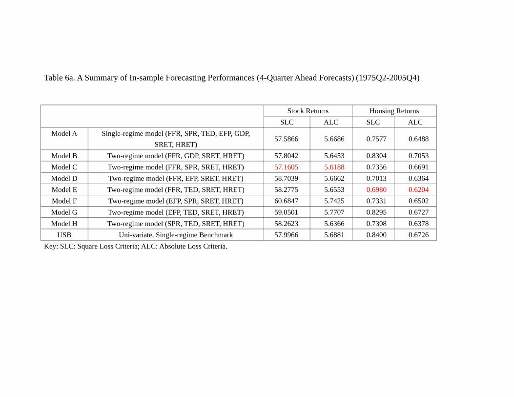
Table 6a. A Summary of In-sample Forecasting Performances (4-Quarter Ahead Forecasts) (1975Q2-2005Q4)

Stock Returns Housing Returns

SLC ALC SLC ALC Model A Single-regime model (FFR, SPR, TED, EFP, GDP,

SRET, HRET) 57.5866 5.6686 0.7577 0.6488

Model B Two-regime model (FFR, GDP, SRET, HRET) 57.8042 5.6453 0.8304 0.7053 Model C Two-regime model (FFR, SPR, SRET, HRET) 57.1605 5.6188 0.7356 0.6691 Model D Two-regime model (FFR, EFP, SRET, HRET) 58.7039 5.6662 0.7013 0.6364 Model E Two-regime model (FFR, TED, SRET, HRET) 58.2775 5.6553 0.6980 0.6204 Model F Two-regime model (EFP, SPR, SRET, HRET) 60.6847 5.7425 0.7331 0.6502 Model G Two-regime model (EFP, TED, SRET, HRET) 59.0501 5.7707 0.8295 0.6727 Model H Two-regime model (SPR, TED, SRET, HRET) 58.2623 5.6366 0.7308 0.6378

USB Uni-variate, Single-regime Benchmark 57.9966 5.6881 0.8400 0.6726 Key: SLC: Square Loss Criteria; ALC: Absolute Loss Criteria.

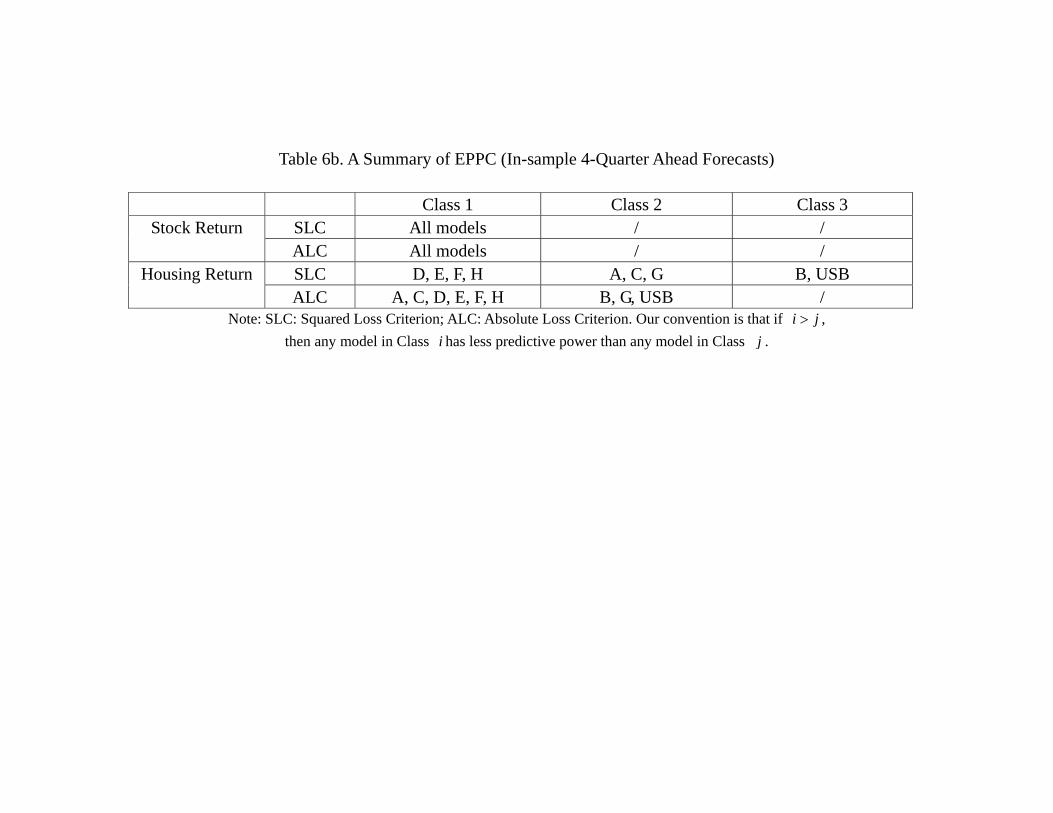
Table 6b. A Summary of EPPC (In-sample 4-Quarter Ahead Forecasts)

Class 1 Class 2 Class 3 Stock Return SLC All models / /

ALC All models / / Housing Return SLC D, E, F, H A, C, G B, USB

ALC A, C, D, E, F, H B, G, USB / Note: SLC: Squared Loss Criterion; ALC: Absolute Loss Criterion. Our convention is that if i j ,

then any model in Class i has less predictive power than any model in Class j .

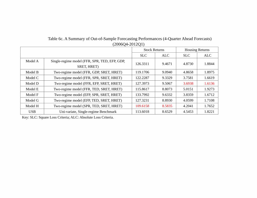
Table 6c. A Summary of Out-of-Sample Forecasting Performances (4-Quarter Ahead Forecasts) (2006Q4-2012Q1)

Stock Returns Housing Returns SLC ALC SLC ALC

Model A Single-regime model (FFR, SPR, TED, EFP, GDP, SRET, HRET)

126.3311 9.4671 4.8730 1.8844



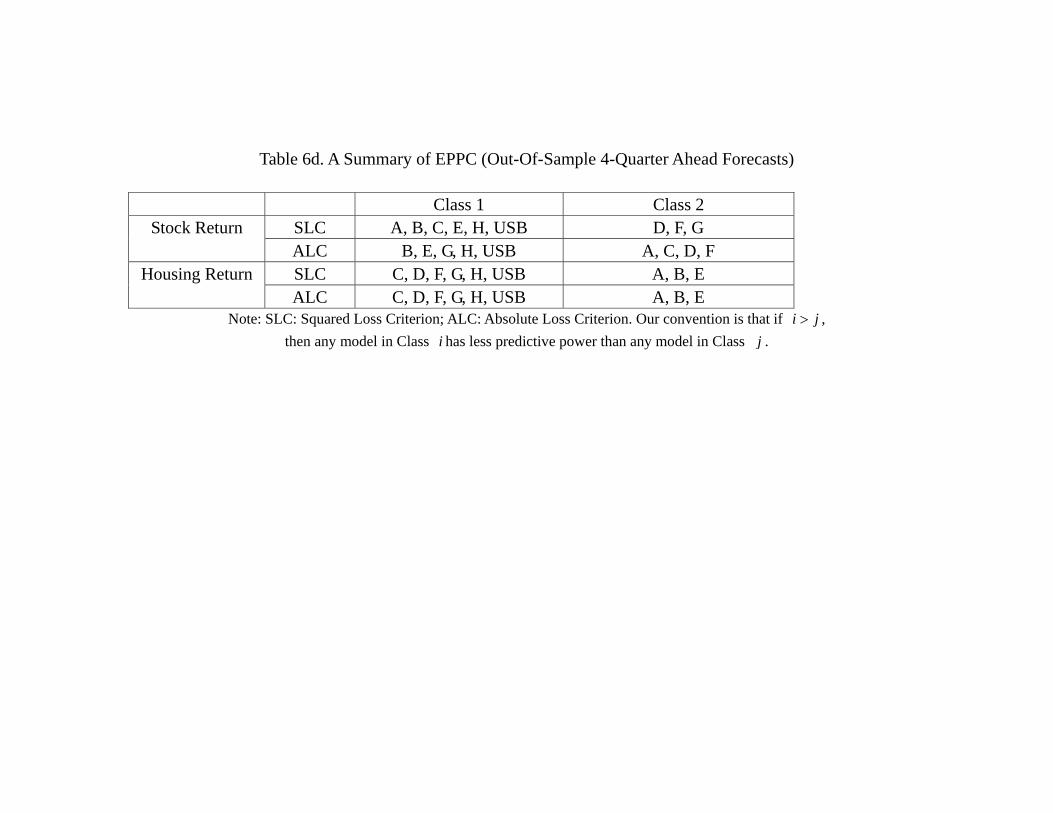
Table 6d. A Summary of EPPC (Out-Of-Sample 4-Quarter Ahead Forecasts)

Class 1 Class 2 Stock Return SLC A, B, C, E, H, USB D, F, G

ALC B, E, G, H, USB A, C, D, F Housing Return SLC C, D, F, G, H, USB A, B, E

ALC C, D, F, G, H, USB A, B, E Note: SLC: Squared Loss Criterion; ALC: Absolute Loss Criterion. Our convention is that if i j ,


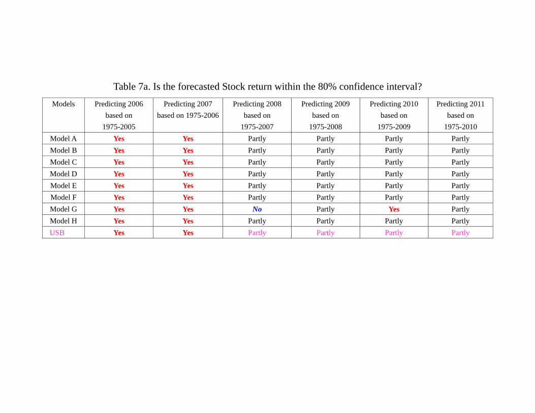
Table 7a. Is the forecasted Stock return within the 80% confidence interval?

Models Predicting 2006 based on

1975-2005

Predicting 2007 based on 1975-2006

Predicting 2008 based on

1975-2007


1975-2008


1975-2009


1975-2010 Model A Yes Yes Partly Partly Partly Partly Model B Yes Yes Partly Partly Partly Partly Model C Yes Yes Partly Partly Partly Partly Model D Yes Yes Partly Partly Partly Partly Model E Yes Yes Partly Partly Partly Partly Model F Yes Yes Partly Partly Partly Partly Model G Yes Yes No Partly Yes Partly Model H Yes Yes Partly Partly Partly Partly USB Yes Yes Partly Partly Partly Partly

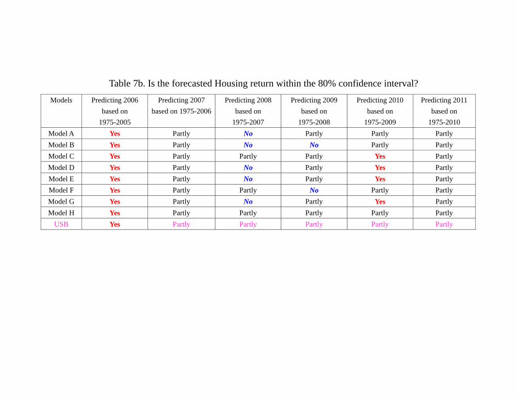
Table 7b. Is the forecasted Housing return within the 80% confidence interval? Models Predicting 2006

based on 1975-2005

Predicting 2007 based on 1975-2006


1975-2007


1975-2008


1975-2009


1975-2010 Model A Yes Partly No Partly Partly Partly Model B Yes Partly No No Partly Partly Model C Yes Partly Partly Partly Yes Partly Model D Yes Partly No Partly Yes Partly Model E Yes Partly No Partly Yes Partly Model F Yes Partly Partly No Partly Partly Model G Yes Partly No Partly Yes Partly Model H Yes Partly Partly Partly Partly Partly

USB Yes Partly Partly Partly Partly Partly

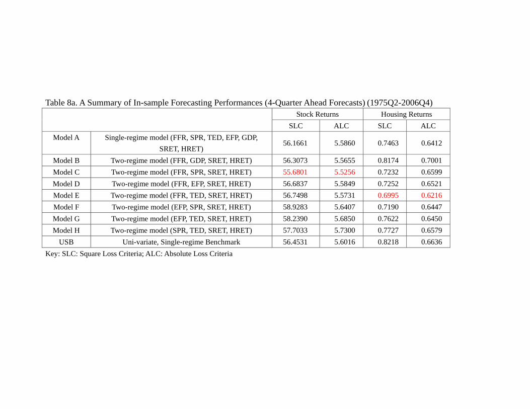
Table 8a. A Summary of In-sample Forecasting Performances (4-Quarter Ahead Forecasts) (1975Q2-2006Q4) Stock Returns Housing Returns

SLC ALC SLC ALC Model A Single-regime model (FFR, SPR, TED, EFP, GDP,

SRET, HRET) 56.1661 5.5860 0.7463 0.6412


USB Uni-variate, Single-regime Benchmark 56.4531 5.6016 0.8218 0.6636 Key: SLC: Square Loss Criteria; ALC: Absolute Loss Criteria

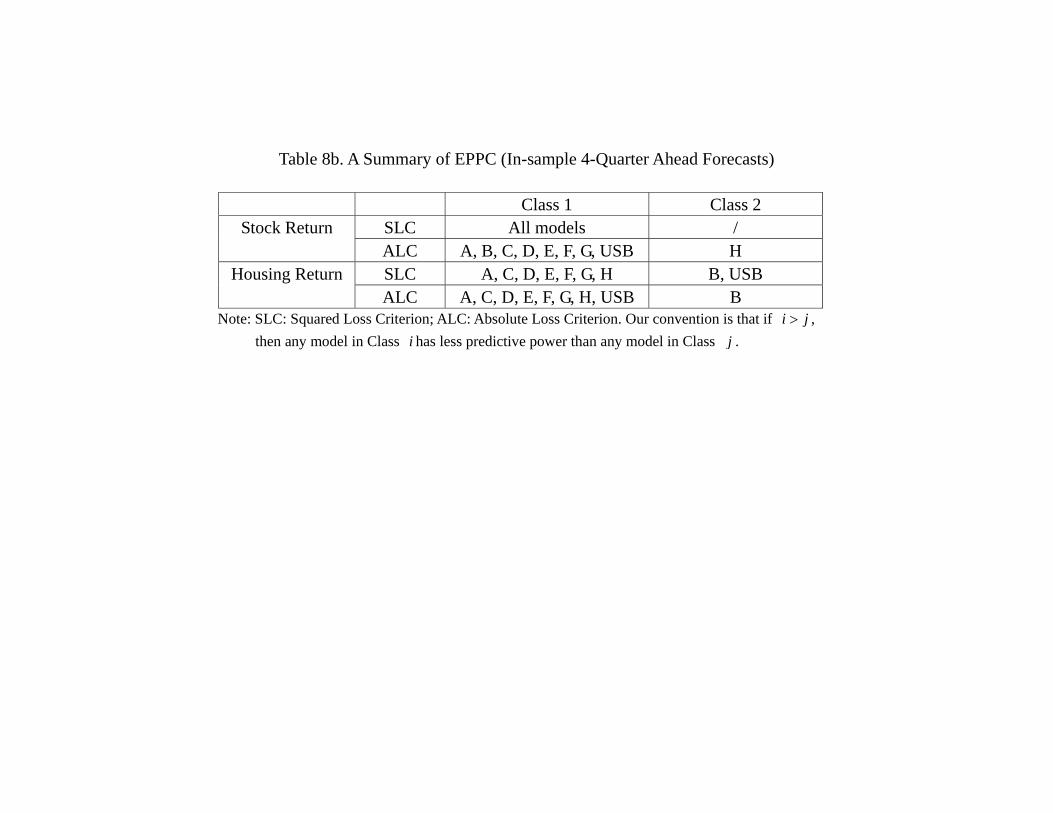
Table 8b. A Summary of EPPC (In-sample 4-Quarter Ahead Forecasts)

Class 1 Class 2 Stock Return SLC All models /

ALC A, B, C, D, E, F, G, USB H Housing Return SLC A, C, D, E, F, G, H B, USB

ALC A, C, D, E, F, G, H, USB B Note: SLC: Squared Loss Criterion; ALC: Absolute Loss Criterion. Our convention is that if i j ,


Table 8c. A Summary of Out-of-Sample Forecasting Performances (4-Quarter Ahead Forecasts) (2007Q4-2012Q1)


Model A Single-regime model (FFR, SPR, TED, EFP, GDP, SRET, HRET)

152.4294 11.0135 5.3034 1.9487



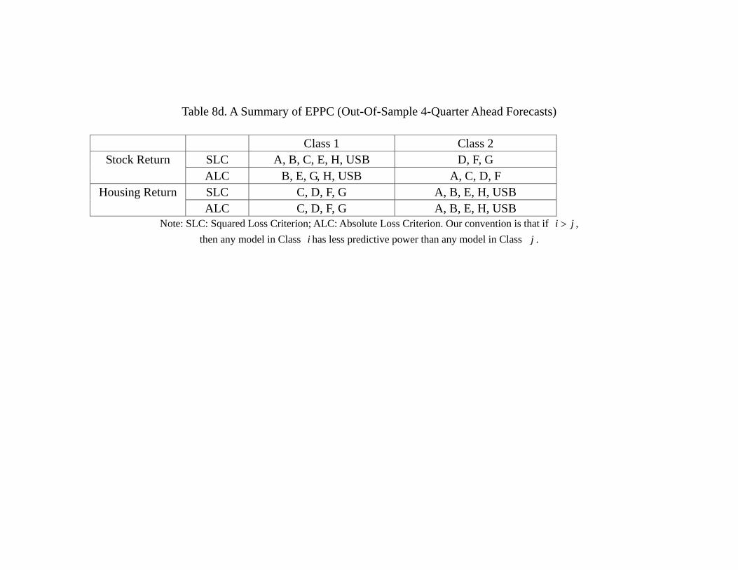
Table 8d. A Summary of EPPC (Out-Of-Sample 4-Quarter Ahead Forecasts)

Class 1 Class 2 Stock Return SLC A, B, C, E, H, USB D, F, G

ALC B, E, G, H, USB A, C, D, F Housing Return SLC C, D, F, G A, B, E, H, USB

ALC C, D, F, G A, B, E, H, USB Note: SLC: Squared Loss Criterion; ALC: Absolute Loss Criterion. Our convention is that if i j ,


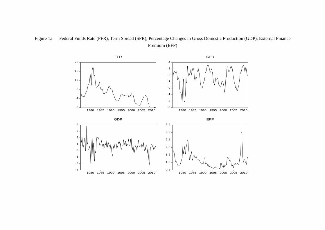
Figure 1a Federal Funds Rate (FFR), Term Spread (SPR), Percentage Changes in Gross Domestic Production (GDP), External Finance Premium (EFP)

0

4

8

12

16

20

1980 1985 1990 1995 2000 2005 2010

FFR

-3

-2

-1

0

1

2

3

4

1980 1985 1990 1995 2000 2005 2010

SPR

-3

-2

-1

0

1

2

3

4

1980 1985 1990 1995 2000 2005 2010

GDP

0.5

1.0

1.5

2.0

2.5

3.0

3.5

1980 1985 1990 1995 2000 2005 2010

EFP

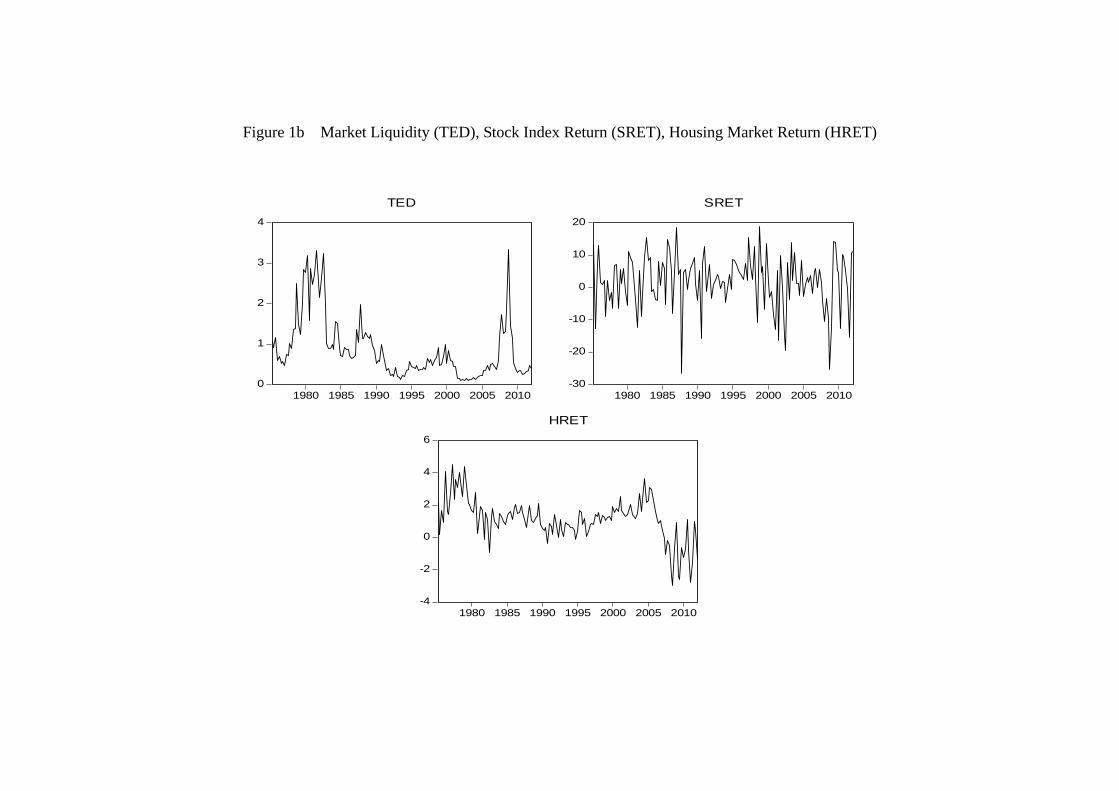
Figure 1b Market Liquidity (TED), Stock Index Return (SRET), Housing Market Return (HRET)

0

1

2

3

4

1980 1985 1990 1995 2000 2005 2010

TED

-30

-20

-10

0

10

20

1980 1985 1990 1995 2000 2005 2010

SRET

-4

-2

0

2

4

6

1980 1985 1990 1995 2000 2005 2010

HRET

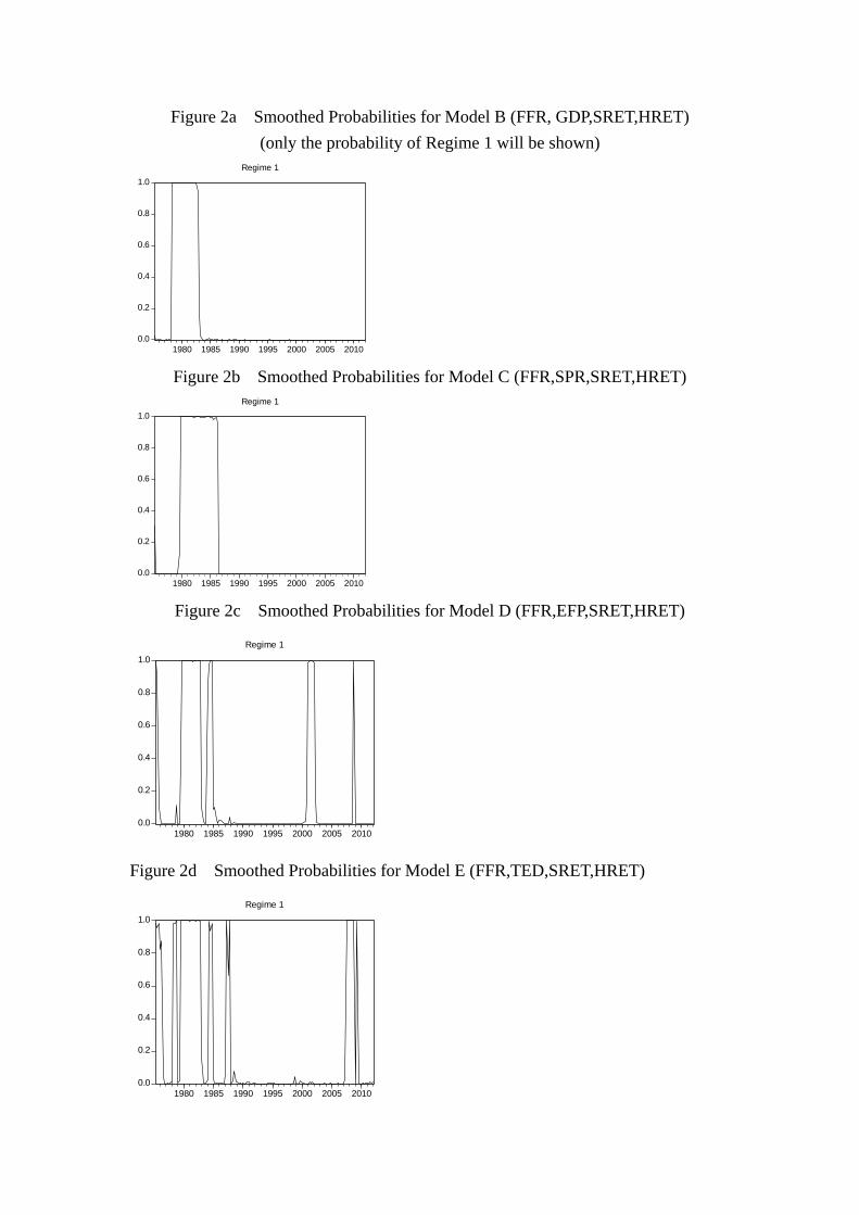
Figure 2a Smoothed Probabilities for Model B (FFR, GDP,SRET,HRET) (only the probability of Regime 1 will be shown)

0.0

0.2

0.4

0.6

0.8

1.0

1980 1985 1990 1995 2000 2005 2010

Regime 1

Figure 2b Smoothed Probabilities for Model C (FFR,SPR,SRET,HRET)

0.0

0.2

0.4

0.6

0.8

1.0

1980 1985 1990 1995 2000 2005 2010

Regime 1

Figure 2c Smoothed Probabilities for Model D (FFR,EFP,SRET,HRET)

0.0

0.2

0.4

0.6

0.8

1.0

1980 1985 1990 1995 2000 2005 2010

Regime 1

Figure 2d Smoothed Probabilities for Model E (FFR,TED,SRET,HRET)

0.0

0.2

0.4

0.6

0.8

1.0

1980 1985 1990 1995 2000 2005 2010

Regime 1

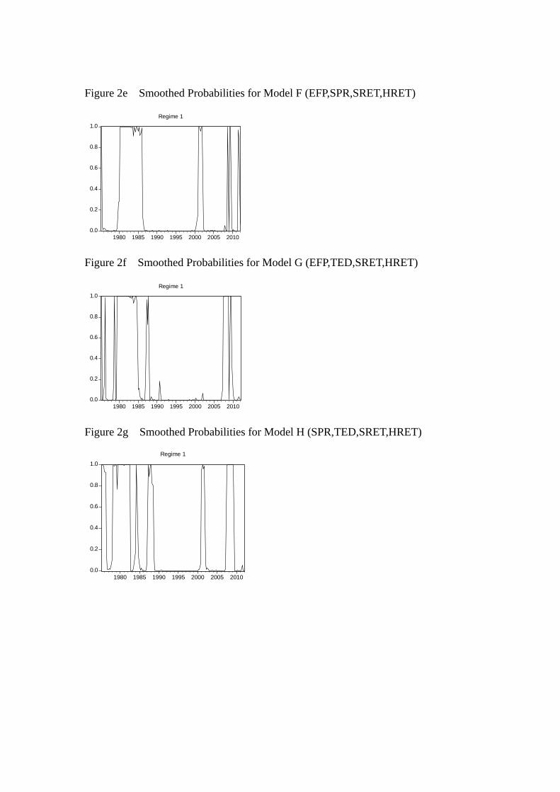
Figure 2e Smoothed Probabilities for Model F (EFP,SPR,SRET,HRET)

0.0

0.2

0.4

0.6

0.8

1.0

1980 1985 1990 1995 2000 2005 2010

Regime 1

Figure 2f Smoothed Probabilities for Model G (EFP,TED,SRET,HRET)

0.0

0.2

0.4

0.6

0.8

1.0

1980 1985 1990 1995 2000 2005 2010

Regime 1

Figure 2g Smoothed Probabilities for Model H (SPR,TED,SRET,HRET)

0.0

0.2

0.4

0.6

0.8

1.0

1980 1985 1990 1995 2000 2005 2010

Regime 1

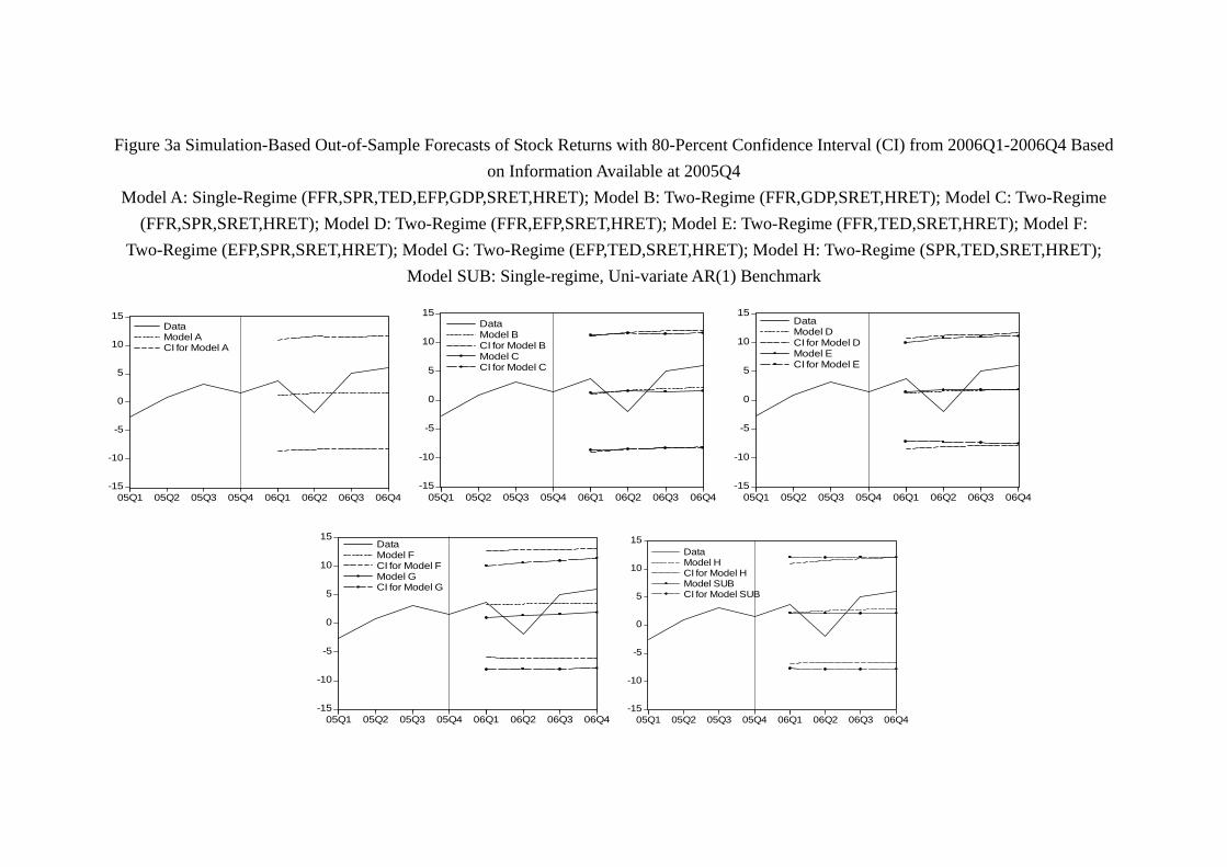
Figure 3a Simulation-Based Out-of-Sample Forecasts of Stock Returns with 80-Percent Confidence Interval (CI) from 2006Q1-2006Q4 Based on Information Available at 2005Q4

Model A: Single-Regime (FFR,SPR,TED,EFP,GDP,SRET,HRET); Model B: Two-Regime (FFR,GDP,SRET,HRET); Model C: Two-Regime (FFR,SPR,SRET,HRET); Model D: Two-Regime (FFR,EFP,SRET,HRET); Model E: Two-Regime (FFR,TED,SRET,HRET); Model F:

Two-Regime (EFP,SPR,SRET,HRET); Model G: Two-Regime (EFP,TED,SRET,HRET); Model H: Two-Regime (SPR,TED,SRET,HRET); Model SUB: Single-regime, Uni-variate AR(1) Benchmark

-15

-10

-5

0

5

10

15

05Q1 05Q2 05Q3 05Q4 06Q1 06Q2 06Q3 06Q4

DataModel ACI for Model A

-15

-10

-5

0

5

10

15

05Q1 05Q2 05Q3 05Q4 06Q1 06Q2 06Q3 06Q4

DataModel BCI for Model BModel CCI for Model C

-15

-10

-5

0

5

10

15

05Q1 05Q2 05Q3 05Q4 06Q1 06Q2 06Q3 06Q4

DataModel DCI for Model DModel ECI for Model E

-15

-10

-5

0

5

10

15

05Q1 05Q2 05Q3 05Q4 06Q1 06Q2 06Q3 06Q4

DataModel FCI for Model FModel GCI for Model G

-15

-10

-5

0

5

10

15

05Q1 05Q2 05Q3 05Q4 06Q1 06Q2 06Q3 06Q4

DataModel HCI for Model HModel SUBCI for Model SUB

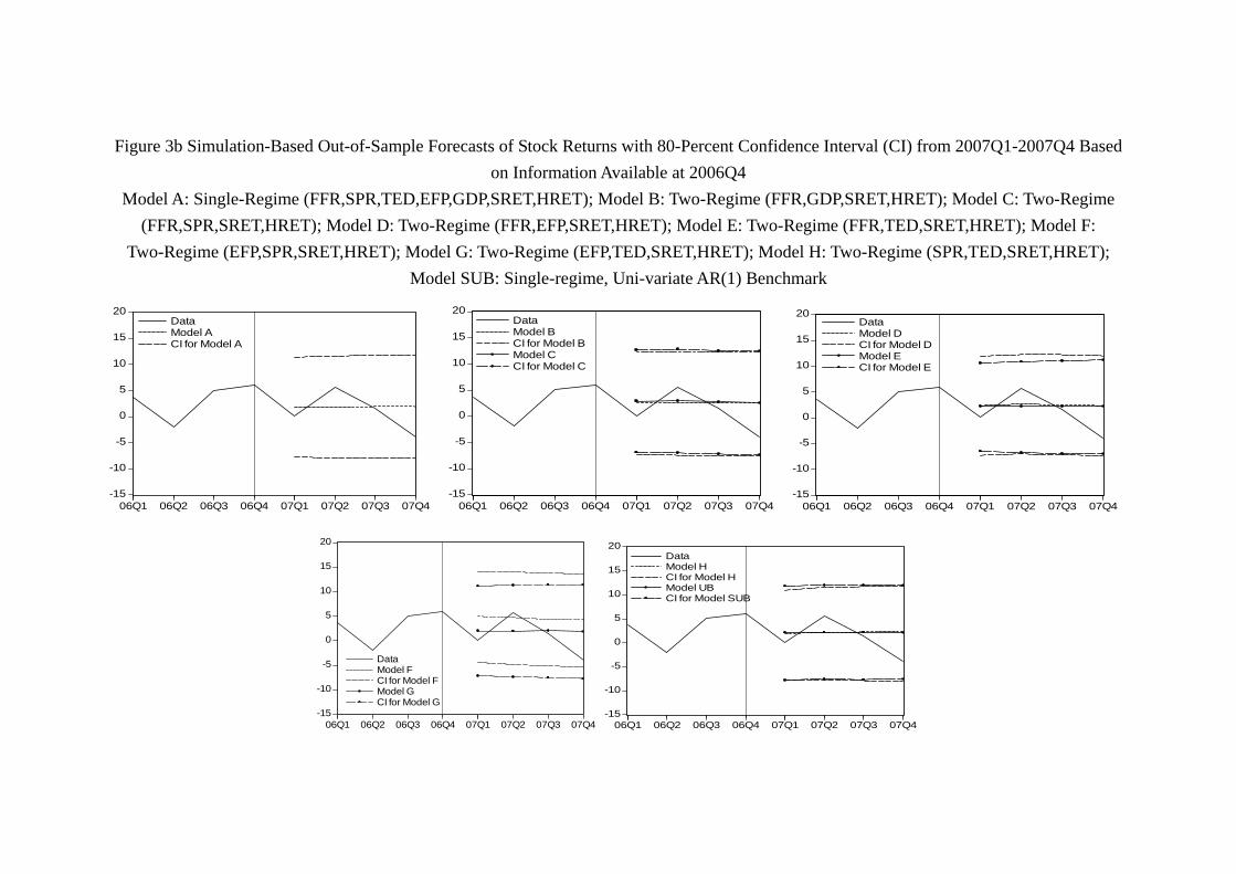
Figure 3b Simulation-Based Out-of-Sample Forecasts of Stock Returns with 80-Percent Confidence Interval (CI) from 2007Q1-2007Q4 Based on Information Available at 2006Q4



-15

-10

-5

0

5

10

15

20

06Q1 06Q2 06Q3 06Q4 07Q1 07Q2 07Q3 07Q4


-15

-10

-5

0

5

10

15

20

06Q1 06Q2 06Q3 06Q4 07Q1 07Q2 07Q3 07Q4


-15

-10

-5

0

5

10

15

20

06Q1 06Q2 06Q3 06Q4 07Q1 07Q2 07Q3 07Q4


-15

-10

-5

0

5

10

15

20

06Q1 06Q2 06Q3 06Q4 07Q1 07Q2 07Q3 07Q4


-15

-10

-5

0

5

10

15

20

06Q1 06Q2 06Q3 06Q4 07Q1 07Q2 07Q3 07Q4

DataModel HCI for Model HModel UBCI for Model SUB

Figure 3c Simulation-Based Out-of-Sample Forecasts of Stock Returns with 80-Percent Confidence Interval (CI) from 2008Q1-2008Q4 Based on Information Available at 2007Q4



-30

-20

-10

0

10

20

30

07Q1 07Q2 07Q3 07Q4 08Q1 08Q2 08Q3 08Q4


-30

-20

-10

0

10

20

30

07Q1 07Q2 07Q3 07Q4 08Q1 08Q2 08Q3 08Q4


-30

-20

-10

0

10

20

30

07Q1 07Q2 07Q3 07Q4 08Q1 08Q2 08Q3 08Q4


-30

-20

-10

0

10

20

30

07Q1 07Q2 07Q3 07Q4 08Q1 08Q2 08Q3 08Q4


-30

-20

-10

0

10

20

30

07Q1 07Q2 07Q3 07Q4 08Q1 08Q2 08Q3 08Q4


Figure 3d Simulation-Based Out-of-Sample Forecasts of Stock Returns with 80-Percent Confidence Interval (CI) from 2009Q1-2009Q4 Based on Information Available at 2008Q4



-30

-20

-10

0

10

20

30

08Q1 08Q2 08Q3 08Q4 09Q1 09Q2 09Q3 09Q4


-30

-20

-10

0

10

20

30

08Q1 08Q2 08Q3 08Q4 09Q1 09Q2 09Q3 09Q4


-30

-20

-10

0

10

20

30

08Q1 08Q2 08Q3 08Q4 09Q1 09Q2 09Q3 09Q4


-30

-20

-10

0

10

20

30

08Q1 08Q2 08Q3 08Q4 09Q1 09Q2 09Q3 09Q4


-30

-20

-10

0

10

20

30

08Q1 08Q2 08Q3 08Q4 09Q1 09Q2 09Q3 09Q4


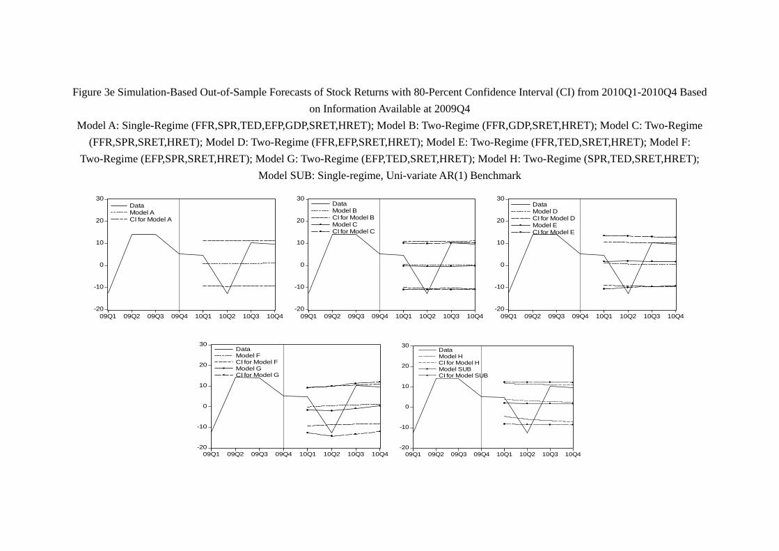
Figure 3e Simulation-Based Out-of-Sample Forecasts of Stock Returns with 80-Percent Confidence Interval (CI) from 2010Q1-2010Q4 Based on Information Available at 2009Q4



-20

-10

0

10

20

30

09Q1 09Q2 09Q3 09Q4 10Q1 10Q2 10Q3 10Q4


-20

-10

0

10

20

30

09Q1 09Q2 09Q3 09Q4 10Q1 10Q2 10Q3 10Q4


-20

-10

0

10

20

30

09Q1 09Q2 09Q3 09Q4 10Q1 10Q2 10Q3 10Q4


-20

-10

0

10

20

30

09Q1 09Q2 09Q3 09Q4 10Q1 10Q2 10Q3 10Q4


-20

-10

0

10

20

30

09Q1 09Q2 09Q3 09Q4 10Q1 10Q2 10Q3 10Q4


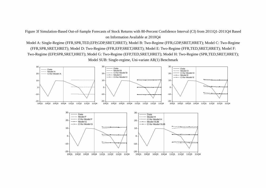
Figure 3f Simulation-Based Out-of-Sample Forecasts of Stock Returns with 80-Percent Confidence Interval (CI) from 2011Q1-2011Q4 Based on Information Available at 2010Q4



-20

-10

0

10

20

30

10Q1 10Q2 10Q3 10Q4 11Q1 11Q2 11Q3 11Q4


-20

-10

0

10

20

30

10Q1 10Q2 10Q3 10Q4 11Q1 11Q2 11Q3 11Q4


-20

-10

0

10

20

30

10Q1 10Q2 10Q3 10Q4 11Q1 11Q2 11Q3 11Q4


-20

-10

0

10

20

30

10Q1 10Q2 10Q3 10Q4 11Q1 11Q2 11Q3 11Q4


-20

-10

0

10

20

30

10Q1 10Q2 10Q3 10Q4 11Q1 11Q2 11Q3 11Q4


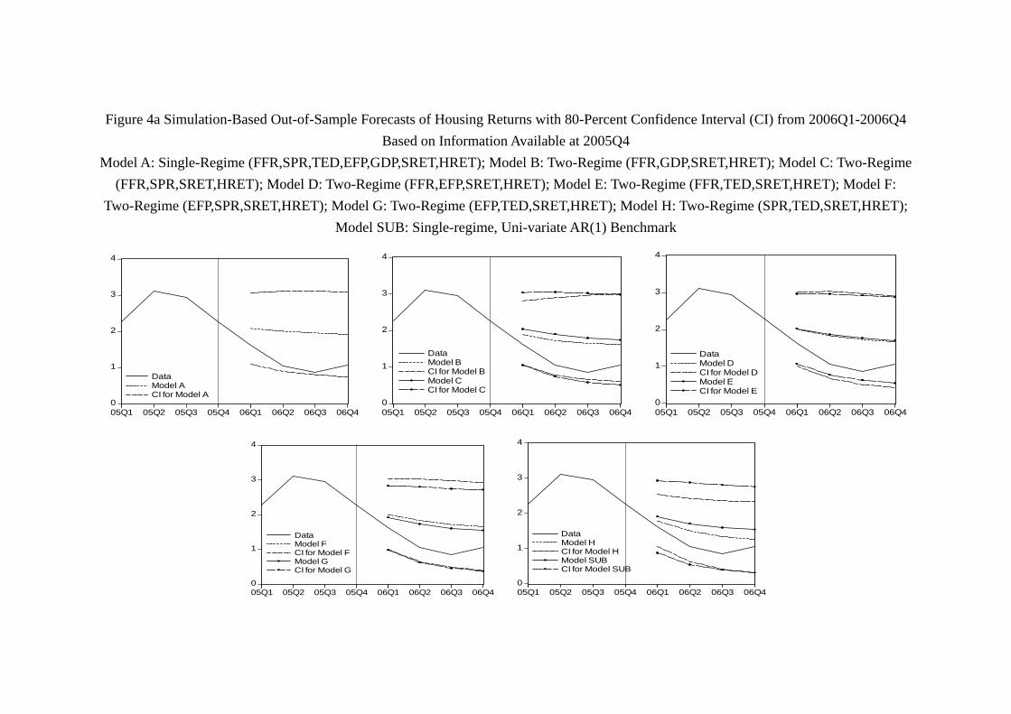
Figure 4a Simulation-Based Out-of-Sample Forecasts of Housing Returns with 80-Percent Confidence Interval (CI) from 2006Q1-2006Q4 Based on Information Available at 2005Q4



0

1

2

3

4

05Q1 05Q2 05Q3 05Q4 06Q1 06Q2 06Q3 06Q4


0

1

2

3

4

05Q1 05Q2 05Q3 05Q4 06Q1 06Q2 06Q3 06Q4


0

1

2

3

4

05Q1 05Q2 05Q3 05Q4 06Q1 06Q2 06Q3 06Q4


0

1

2

3

4

05Q1 05Q2 05Q3 05Q4 06Q1 06Q2 06Q3 06Q4


0

1

2

3

4

05Q1 05Q2 05Q3 05Q4 06Q1 06Q2 06Q3 06Q4


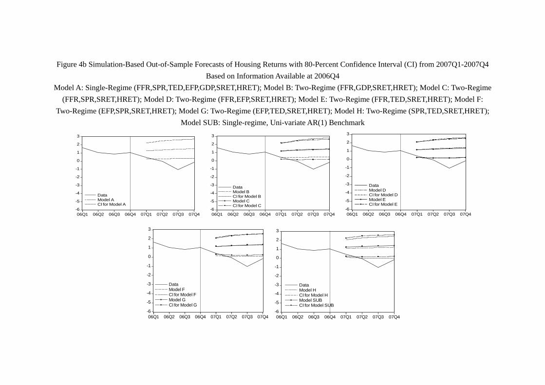
Figure 4b Simulation-Based Out-of-Sample Forecasts of Housing Returns with 80-Percent Confidence Interval (CI) from 2007Q1-2007Q4 Based on Information Available at 2006Q4



-6

-5

-4

-3

-2

-1

0

1

2

3

06Q1 06Q2 06Q3 06Q4 07Q1 07Q2 07Q3 07Q4


-6

-5

-4

-3

-2

-1

0

1

2

3

06Q1 06Q2 06Q3 06Q4 07Q1 07Q2 07Q3 07Q4


-6

-5

-4

-3

-2

-1

0

1

2

3

06Q1 06Q2 06Q3 06Q4 07Q1 07Q2 07Q3 07Q4


-6

-5

-4

-3

-2

-1

0

1

2

3

06Q1 06Q2 06Q3 06Q4 07Q1 07Q2 07Q3 07Q4


-6

-5

-4

-3

-2

-1

0

1

2

3

06Q1 06Q2 06Q3 06Q4 07Q1 07Q2 07Q3 07Q4


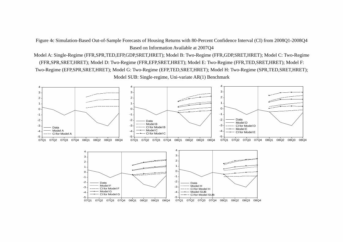
Figure 4c Simulation-Based Out-of-Sample Forecasts of Housing Returns with 80-Percent Confidence Interval (CI) from 2008Q1-2008Q4 Based on Information Available at 2007Q4



-5

-4

-3

-2

-1

0

1

2

3

4

07Q1 07Q2 07Q3 07Q4 08Q1 08Q2 08Q3 08Q4


-5

-4

-3

-2

-1

0

1

2

3

4

07Q1 07Q2 07Q3 07Q4 08Q1 08Q2 08Q3 08Q4


-5

-4

-3

-2

-1

0

1

2

3

4

07Q1 07Q2 07Q3 07Q4 08Q1 08Q2 08Q3 08Q4


-5

-4

-3

-2

-1

0

1

2

3

4

07Q1 07Q2 07Q3 07Q4 08Q1 08Q2 08Q3 08Q4


-5

-4

-3

-2

-1

0

1

2

3

4

07Q1 07Q2 07Q3 07Q4 08Q1 08Q2 08Q3 08Q4


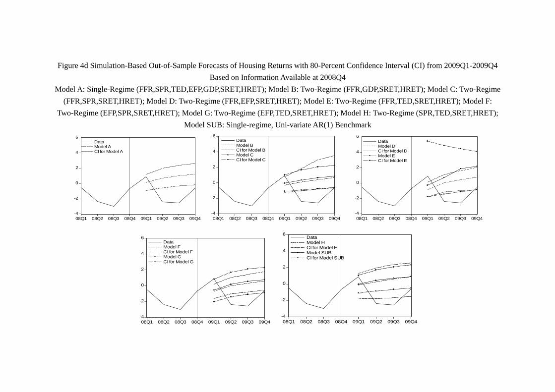
Figure 4d Simulation-Based Out-of-Sample Forecasts of Housing Returns with 80-Percent Confidence Interval (CI) from 2009Q1-2009Q4 Based on Information Available at 2008Q4



-4

-2

0

2

4

6

08Q1 08Q2 08Q3 08Q4 09Q1 09Q2 09Q3 09Q4


-4

-2

0

2

4

6

08Q1 08Q2 08Q3 08Q4 09Q1 09Q2 09Q3 09Q4


-4

-2

0

2

4

6

08Q1 08Q2 08Q3 08Q4 09Q1 09Q2 09Q3 09Q4


-4

-2

0

2

4

6

08Q1 08Q2 08Q3 08Q4 09Q1 09Q2 09Q3 09Q4


-4

-2

0

2

4

6

08Q1 08Q2 08Q3 08Q4 09Q1 09Q2 09Q3 09Q4


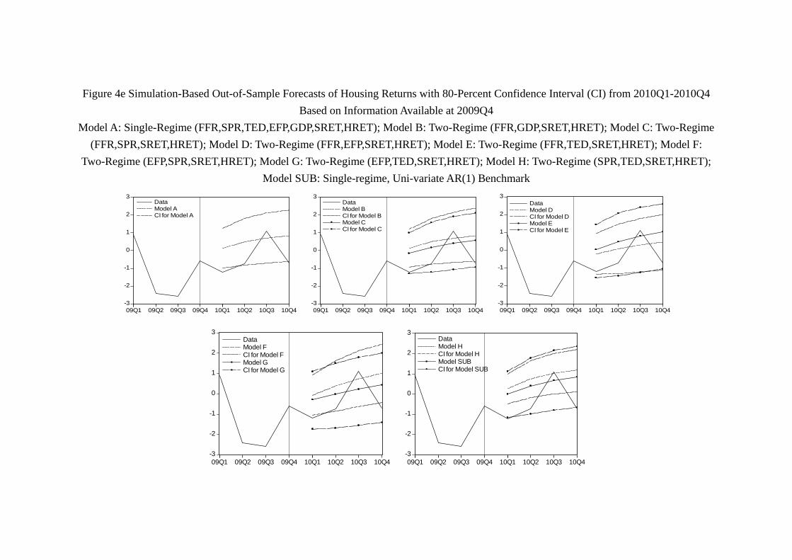
Figure 4e Simulation-Based Out-of-Sample Forecasts of Housing Returns with 80-Percent Confidence Interval (CI) from 2010Q1-2010Q4 Based on Information Available at 2009Q4



-3

-2

-1

0

1

2

3

09Q1 09Q2 09Q3 09Q4 10Q1 10Q2 10Q3 10Q4


-3

-2

-1

0

1

2

3

09Q1 09Q2 09Q3 09Q4 10Q1 10Q2 10Q3 10Q4


-3

-2

-1

0

1

2

3

09Q1 09Q2 09Q3 09Q4 10Q1 10Q2 10Q3 10Q4


-3

-2

-1

0

1

2

3

09Q1 09Q2 09Q3 09Q4 10Q1 10Q2 10Q3 10Q4


-3

-2

-1

0

1

2

3

09Q1 09Q2 09Q3 09Q4 10Q1 10Q2 10Q3 10Q4


Figure 4f Simulation-Based Out-of-Sample Forecasts of Housing Returns with 80-Percent Confidence Interval (CI) from 2011Q1-2011Q4 Based on Information Available at 2010Q4



-3

-2

-1

0

1

2

3

10Q1 10Q2 10Q3 10Q4 11Q1 11Q2 11Q3 11Q4


-3

-2

-1

0

1

2

3

10Q1 10Q2 10Q3 10Q4 11Q1 11Q2 11Q3 11Q4


-3

-2

-1

0

1

2

3

10Q1 10Q2 10Q3 10Q4 11Q1 11Q2 11Q3 11Q4


-3

-2

-1

0

1

2

3

10Q1 10Q2 10Q3 10Q4 11Q1 11Q2 11Q3 11Q4


-3

-2

-1

0

1

2

3

10Q1 10Q2 10Q3 10Q4 11Q1 11Q2 11Q3 11Q4


Losing track of the asset markets: the case of housing and stock (April 2015) APPENDIX

We are grateful to all suggestions and feedback. In response, we provide more details and some supplementary results in this appendix, which has different parts. Appendix A provides the details of the estimation results. Appendix B provides the non-stationarity test for the regime-switching models. Appendix C provides the results of the Diebold-Mariano tests. Appendix D provides the LM test results of the residuals from different models. Appendix E discusses the suggestion of using Case-Shiller index. Appendix F shows that the consideration of mortgage rate may not be necessary once our variables, such as FFR, and others are included. Appendix G shows all the graphs of smoothed probabilities for different regimes in different models. Appendix H provides the detailed results of the Mariano-Preve test. Appendix I provides a simple review of the literature which chooses a similar boom-bust date as we do. Appendix J provides the detailed results when the in-sample is chosen to be 1975 to 2006. Appendix K provides the detailed results when the in-sample is chosen to be 1975 to 2007.

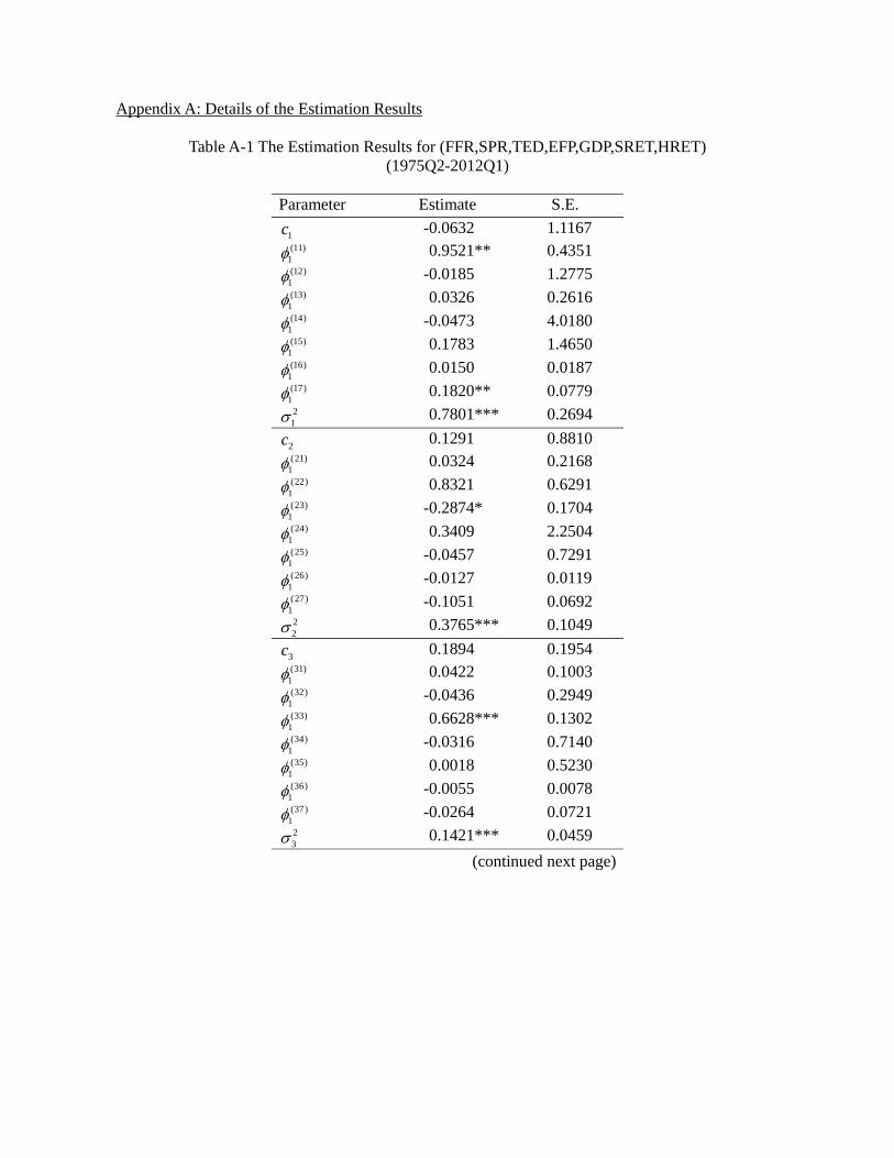
Appendix A: Details of the Estimation Results

Table A-1 The Estimation Results for (FFR,SPR,TED,EFP,GDP,SRET,HRET) (1975Q2-2012Q1)

Parameter Estimate S.E.

1c -0.0632 1.1167 (11)

1 0.9521** 0.4351 (12)

1 -0.0185 1.2775 (13)

1 0.0326 0.2616 (14)

1 -0.0473 4.0180 (15)

1 0.1783 1.4650 (16)

1 0.0150 0.0187 (17)

1 0.1820** 0.0779 21 0.7801*** 0.2694

2c 0.1291 0.8810 (21)

1 0.0324 0.2168 (22)

1 0.8321 0.6291 (23)

1 -0.2874* 0.1704 (24)

1 0.3409 2.2504 (25)

1 -0.0457 0.7291 (26)

1 -0.0127 0.0119 (27)

1 -0.1051 0.0692 22 0.3765*** 0.1049

3c 0.1894 0.1954 (31)

1 0.0422 0.1003 (32)

1 -0.0436 0.2949 (33)

1 0.6628*** 0.1302 (34)

1 -0.0316 0.7140 (35)

1 0.0018 0.5230 (36)

1 -0.0055 0.0078 (37)

1 -0.0264 0.0721 23 0.1421*** 0.0459

(continued next page)

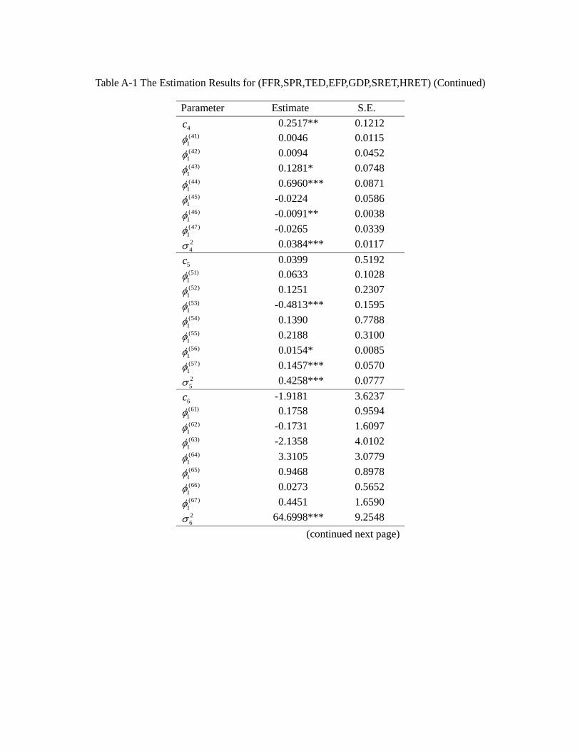
Table A-1 The Estimation Results for (FFR,SPR,TED,EFP,GDP,SRET,HRET) (Continued)


4c 0.2517** 0.1212 (41)

1 0.0046 0.0115 (42)

1 0.0094 0.0452 (43)

1 0.1281* 0.0748 (44)

1 0.6960*** 0.0871 (45)

1 -0.0224 0.0586 (46)

1 -0.0091** 0.0038 (47)

1 -0.0265 0.0339 24 0.0384*** 0.0117

5c 0.0399 0.5192 (51)

1 0.0633 0.1028 (52)

1 0.1251 0.2307 (53)

1 -0.4813*** 0.1595 (54)

1 0.1390 0.7788 (55)

1 0.2188 0.3100 (56)

1 0.0154* 0.0085 (57)

1 0.1457*** 0.0570 25 0.4258*** 0.0777

6c -1.9181 3.6237 (61)

1 0.1758 0.9594 (62)

1 -0.1731 1.6097 (63)

1 -2.1358 4.0102 (64)

1 3.3105 3.0779 (65)

1 0.9468 0.8978 (66)

1 0.0273 0.5652 (67)

1 0.4451 1.6590 26 64.6998*** 9.2548


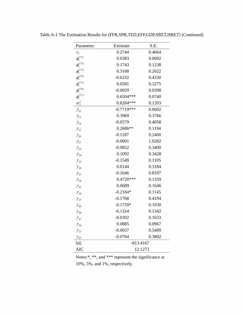
Table A-1 The Estimation Results for (FFR,SPR,TED,EFP,GDP,SRET,HRET) (Continued)


7c 0.2744 0.4664 (71)

1 0.0383 0.0692 (72)

1 0.1743 0.1238 (73)

1 0.3168 0.2622 (74)

1 -0.6332 0.4330 (75)

1 0.0581 0.3275 (76)

1 -0.0029 0.0398 (77)

1 0.6504*** 0.0740 27 0.8264*** 0.1203

12 -0.7719*** 0.0692 13 0.3969 0.3766 14 -0.0579 0.4058 15 0.2686** 0.1194 16 -0.1187 0.2400 17 -0.0001 1.0282 23 -0.0852 0.3400 24 0.1092 0.3428 25 -0.1549 0.1105 26 0.0144 0.3184 27 -0.1646 0.8197 34 0.4720*** 0.1359 35 0.0689 0.1646 36 -0.2184* 0.1145 37 -0.1768 0.4194 45 -0.1759* 0.1030 46 -0.1324 0.1342 47 -0.0302 0.1633 56 0.0885 0.0967 57 -0.0037 0.5499 67 -0.0764 0.3802

lnL -813.4167 AIC 12.1273

Notes:*, **, and *** represent the significance at 10%, 5%, and 1%, respectively.

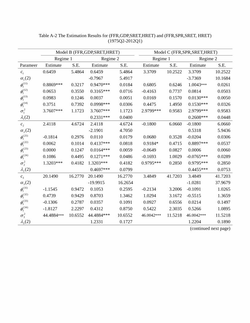
Table A-2 The Estimation Results for (FFR,GDP,SRET,HRET) and (FFR,SPR,SRET, HRET)

(1975Q2-2012Q1)

Model B (FFR,GDP,SRET,HRET) Model C (FFR,SPR,SRET,HRET) Regime 1 Regime 2 Regime 1 Regime 2 Parameer Estimate S.E. Estimate S.E. Estimate S.E. Estimate S.E.

1c 0.6459 5.4864 0.6459 5.4864 3.3709 10.2522 3.3709 10.25221(2) -0.7967 5.4917 -3.7369 10.1684(11)

1 0.8869*** 0.3217 0.9470*** 0.0184 0.6805 0.6246 1.0043*** 0.0261(12)

1 0.0653 0.3550 0.3165*** 0.0716 -0.4163 0.7737 0.0814 0.0503(13)

1 0.0983 0.1246 0.0037 0.0051 0.0169 0.1570 0.0130*** 0.0050(14)

1 0.3751 0.7392 0.0998*** 0.0306 0.4475 1.4950 0.1530*** 0.032621 3.7607*** 1.1723 3.7607*** 1.1723 2.9799*** 0.9583 2.9799*** 0.95831(2) 0.2331*** 0.0400 0.2608*** 0.0448

2c 2.4118 4.6724 2.4118 4.6724 -0.1800 6.0660 -0.1800 6.06602 (2) -2.1901 4.7050 0.5318 5.9436(21)

1 -0.1814 0.2976 0.0110 0.0179 0.0680 0.3528 -0.0204 0.0306(22)

1 0.0062 0.1014 0.4137*** 0.0818 0.9184* 0.4715 0.8897*** 0.0537(23)

1 0.0000 0.1247 0.0164*** 0.0059 -0.0649 0.0827 0.0006 0.0060(24)

1 0.1086 0.4495 0.1271*** 0.0486 -0.1693 1.0029 -0.0765*** 0.028922 1.3203*** 0.4182 1.3203*** 0.4182 0.9795*** 0.2850 0.9795*** 0.28502 (2) 0.4697*** 0.0799 0.4455*** 0.0753

3c 20.1490 16.2770 20.1490 16.2770 3.4849 41.7203 3.4849 41.72033(2) -19.9915 16.2654 -1.0281 37.9679(31)

1 -1.1545 0.9472 0.1053 0.2595 -0.2134 3.2006 -0.1091 1.0265(32)

1 0.4739 0.9429 0.8703 1.3462 1.0294 3.1672 -0.5515 1.3659(33)

1 -0.1306 0.2787 0.0357 0.1091 0.0927 0.6556 0.0214 0.1497(34)

1 -1.8127 2.2297 0.4312 0.8750 0.5422 2.3035 0.5266 1.089523 44.4884*** 10.6552 44.4884*** 10.6552 46.0042*** 11.5218 46.0042*** 11.52183 (2) 1.2331 0.1727 1.2204 0.1890


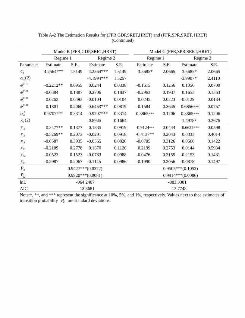
Table A-2 The Estimation Results for (FFR,GDP,SRET,HRET) and (FFR,SPR,SRET, HRET)

(Continued)

Model B (FFR,GDP,SRET,HRET) Model C (FFR,SPR,SRET,HRET) Regime 1 Regime 2 Regime 1 Regime 2 Parameter Estimate S.E. Estimate S.E. Estimate S.E. Estimate S.E.

4c 4.2564*** 1.5149 4.2564*** 1.5149 3.5685* 2.0665 3.5685* 2.0665

4 (2) -4.1994*** 1.5257 -3.9907* 2.4110 (41)

1 -0.2212** 0.0955 0.0244 0.0338 -0.1615 0.1256 0.1056 0.0700 (42)

1 -0.0384 0.1887 0.2706 0.1837 -0.2963 0.1937 0.1653 0.1363 (43)

1 -0.0262 0.0493 -0.0104 0.0104 0.0245 0.0223 -0.0129 0.0134 (44)

1 0.1801 0.2060 0.6453*** 0.0819 -0.1584 0.3645 0.6856*** 0.0757 24 0.9707*** 0.3314 0.9707*** 0.3314 0.3865*** 0.1206 0.3865*** 0.1206

4 (2) 0.8945 0.1664 1.4978* 0.2676

12 0.3477** 0.1377 0.1335 0.0919 -0.9124*** 0.0444 -0.6622*** 0.0598

13 -0.5269** 0.2073 -0.0201 0.0918 -0.4137** 0.2043 0.0333 0.4014

14 -0.0587 0.3935 -0.0565 0.0820 -0.0705 0.3126 0.0660 0.1422

23 -0.2109 0.2778 0.1670 0.1126 0.2199 0.2753 0.0144 0.5934

24 -0.0523 0.1523 -0.0783 0.0988 -0.0476 0.3155 -0.2153 0.1431

34 -0.2987 0.2067 -0.1145 0.0986 -0.1990 0.2056 -0.0878 0.1497

11P 0.9427***(0.0372) 0.9505***(0.1053)

22P 0.9920***(0.0081) 0.9914***(0.0086) lnL -964.2407 -883.3381 AIC 13.8681 12.7748 Note:*, **, and *** represent the significance at 10%, 5%, and 1%, respectively. Values next to thee estimates of transition probability iiP are standard deviations.

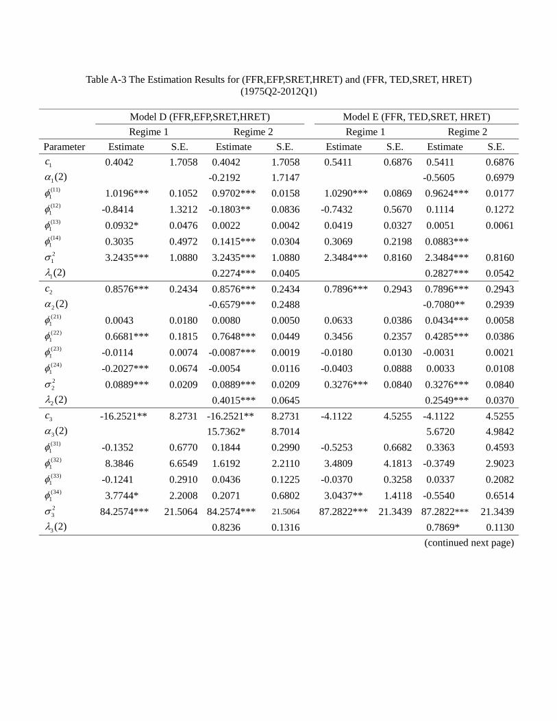
Table A-3 The Estimation Results for (FFR,EFP,SRET,HRET) and (FFR, TED,SRET, HRET)

(1975Q2-2012Q1)

Model D (FFR,EFP,SRET,HRET) Model E (FFR, TED,SRET, HRET) Regime 1 Regime 2 Regime 1 Regime 2 Parameter Estimate S.E. Estimate S.E. Estimate S.E. Estimate S.E.

1c 0.4042 1.7058 0.4042 1.7058 0.5411 0.6876 0.5411 0.6876

1(2) -0.2192 1.7147 -0.5605 0.6979(11)

1 1.0196*** 0.1052 0.9702*** 0.0158 1.0290*** 0.0869 0.9624*** 0.0177(12)

1 -0.8414 1.3212 -0.1803** 0.0836 -0.7432 0.5670 0.1114 0.1272(13)

1 0.0932* 0.0476 0.0022 0.0042 0.0419 0.0327 0.0051 0.0061(14)

1 0.3035 0.4972 0.1415*** 0.0304 0.3069 0.2198 0.0883*** 21 3.2435*** 1.0880 3.2435*** 1.0880 2.3484*** 0.8160 2.3484*** 0.8160

1(2) 0.2274*** 0.0405 0.2827*** 0.0542

2c 0.8576*** 0.2434 0.8576*** 0.2434 0.7896*** 0.2943 0.7896*** 0.2943

2 (2) -0.6579*** 0.2488 -0.7080** 0.2939(21)

1 0.0043 0.0180 0.0080 0.0050 0.0633 0.0386 0.0434*** 0.0058(22)

1 0.6681*** 0.1815 0.7648*** 0.0449 0.3456 0.2357 0.4285*** 0.0386(23)

1 -0.0114 0.0074 -0.0087*** 0.0019 -0.0180 0.0130 -0.0031 0.0021(24)

1 -0.2027*** 0.0674 -0.0054 0.0116 -0.0403 0.0888 0.0033 0.010822 0.0889*** 0.0209 0.0889*** 0.0209 0.3276*** 0.0840 0.3276*** 0.0840

2 (2) 0.4015*** 0.0645 0.2549*** 0.0370

3c -16.2521** 8.2731 -16.2521** 8.2731 -4.1122 4.5255 -4.1122 4.5255

3(2) 15.7362* 8.7014 5.6720 4.9842(31)

1 -0.1352 0.6770 0.1844 0.2990 -0.5253 0.6682 0.3363 0.4593(32)

1 8.3846 6.6549 1.6192 2.2110 3.4809 4.1813 -0.3749 2.9023(33)

1 -0.1241 0.2910 0.0436 0.1225 -0.0370 0.3258 0.0337 0.2082(34)

1 3.7744* 2.2008 0.2071 0.6802 3.0437** 1.4118 -0.5540 0.651423 84.2574*** 21.5064 84.2574*** 21.5064 87.2822*** 21.3439 87.2822*** 21.3439

3(2) 0.8236 0.1316 0.7869* 0.1130(continued next page)

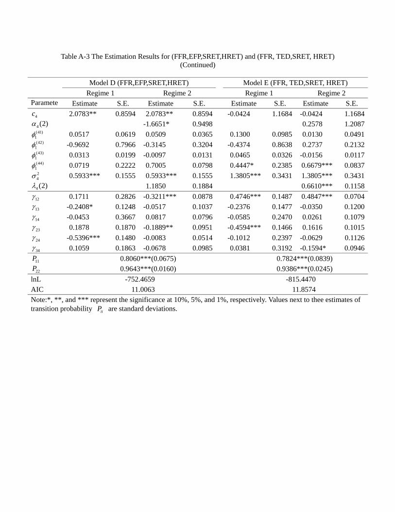
Table A-3 The Estimation Results for (FFR,EFP,SRET,HRET) and (FFR, TED,SRET, HRET)

(Continued)

Model D (FFR,EFP,SRET,HRET) Model E (FFR, TED,SRET, HRET) Regime 1 Regime 2 Regime 1 Regime 2 Paramete Estimate S.E. Estimate S.E. Estimate S.E. Estimate S.E.

4c 2.0783** 0.8594 2.0783** 0.8594 -0.0424 1.1684 -0.0424 1.16844 (2) -1.6651* 0.9498 0.2578 1.2087(41)

1 0.0517 0.0619 0.0509 0.0365 0.1300 0.0985 0.0130 0.0491(42)

1 -0.9692 0.7966 -0.3145 0.3204 -0.4374 0.8638 0.2737 0.2132(43)

1 0.0313 0.0199 -0.0097 0.0131 0.0465 0.0326 -0.0156 0.0117(44)

1 0.0719 0.2222 0.7005 0.0798 0.4447* 0.2385 0.6679*** 0.083724 0.5933*** 0.1555 0.5933*** 0.1555 1.3805*** 0.3431 1.3805*** 0.34314 (2) 1.1850 0.1884 0.6610*** 0.1158

12 0.1711 0.2826 -0.3211*** 0.0878 0.4746*** 0.1487 0.4847*** 0.070413 -0.2408* 0.1248 -0.0517 0.1037 -0.2376 0.1477 -0.0350 0.120014 -0.0453 0.3667 0.0817 0.0796 -0.0585 0.2470 0.0261 0.107923 0.1878 0.1870 -0.1889** 0.0951 -0.4594*** 0.1466 0.1616 0.101524 -0.5396*** 0.1480 -0.0083 0.0514 -0.1012 0.2397 -0.0629 0.112634 0.1059 0.1863 -0.0678 0.0985 0.0381 0.3192 -0.1594* 0.0946

11P 0.8060***(0.0675) 0.7824***(0.0839) 22P 0.9643***(0.0160) 0.9386***(0.0245)

lnL -752.4659 -815.4470 AIC 11.0063 11.8574 Note:*, **, and *** represent the significance at 10%, 5%, and 1%, respectively. Values next to thee estimates of transition probability iiP are standard deviations.

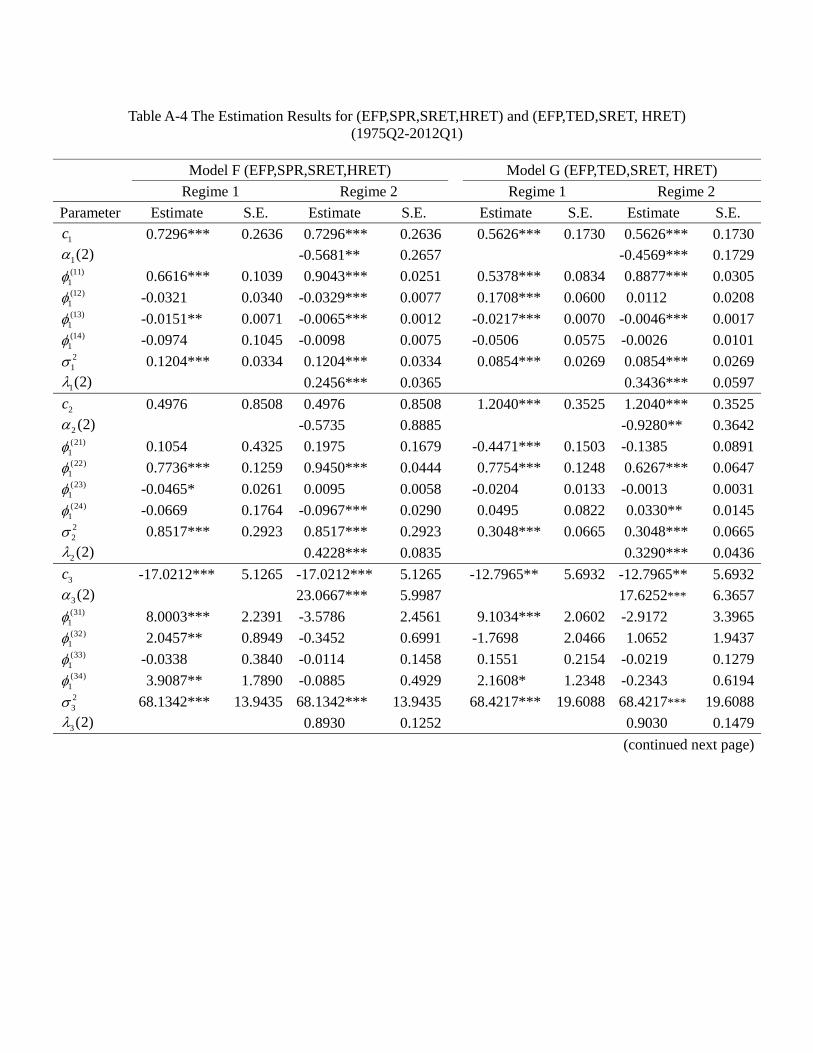
Table A-4 The Estimation Results for (EFP,SPR,SRET,HRET) and (EFP,TED,SRET, HRET)

(1975Q2-2012Q1)

Model F (EFP,SPR,SRET,HRET) Model G (EFP,TED,SRET, HRET) Regime 1 Regime 2 Regime 1 Regime 2 Parameter Estimate S.E. Estimate S.E. Estimate S.E. Estimate S.E.

1c 0.7296*** 0.2636 0.7296*** 0.2636 0.5626*** 0.1730 0.5626*** 0.17301(2) -0.5681** 0.2657 -0.4569*** 0.1729(11)

1 0.6616*** 0.1039 0.9043*** 0.0251 0.5378*** 0.0834 0.8877*** 0.0305(12)

1 -0.0321 0.0340 -0.0329*** 0.0077 0.1708*** 0.0600 0.0112 0.0208(13)

1 -0.0151** 0.0071 -0.0065*** 0.0012 -0.0217*** 0.0070 -0.0046*** 0.0017(14)

1 -0.0974 0.1045 -0.0098 0.0075 -0.0506 0.0575 -0.0026 0.010121 0.1204*** 0.0334 0.1204*** 0.0334 0.0854*** 0.0269 0.0854*** 0.02691(2) 0.2456*** 0.0365 0.3436*** 0.0597

2c 0.4976 0.8508 0.4976 0.8508 1.2040*** 0.3525 1.2040*** 0.35252 (2) -0.5735 0.8885 -0.9280** 0.3642(21)

1 0.1054 0.4325 0.1975 0.1679 -0.4471*** 0.1503 -0.1385 0.0891(22)

1 0.7736*** 0.1259 0.9450*** 0.0444 0.7754*** 0.1248 0.6267*** 0.0647(23)

1 -0.0465* 0.0261 0.0095 0.0058 -0.0204 0.0133 -0.0013 0.0031(24)

1 -0.0669 0.1764 -0.0967*** 0.0290 0.0495 0.0822 0.0330** 0.014522 0.8517*** 0.2923 0.8517*** 0.2923 0.3048*** 0.0665 0.3048*** 0.06652 (2) 0.4228*** 0.0835 0.3290*** 0.0436

3c -17.0212*** 5.1265 -17.0212*** 5.1265 -12.7965** 5.6932 -12.7965** 5.69323(2) 23.0667*** 5.9987 17.6252*** 6.3657(31)

1 8.0003*** 2.2391 -3.5786 2.4561 9.1034*** 2.0602 -2.9172 3.3965(32)

1 2.0457** 0.8949 -0.3452 0.6991 -1.7698 2.0466 1.0652 1.9437(33)

1 -0.0338 0.3840 -0.0114 0.1458 0.1551 0.2154 -0.0219 0.1279(34)

1 3.9087** 1.7890 -0.0885 0.4929 2.1608* 1.2348 -0.2343 0.619423 68.1342*** 13.9435 68.1342*** 13.9435 68.4217*** 19.6088 68.4217*** 19.60883(2) 0.8930 0.1252 0.9030 0.1479


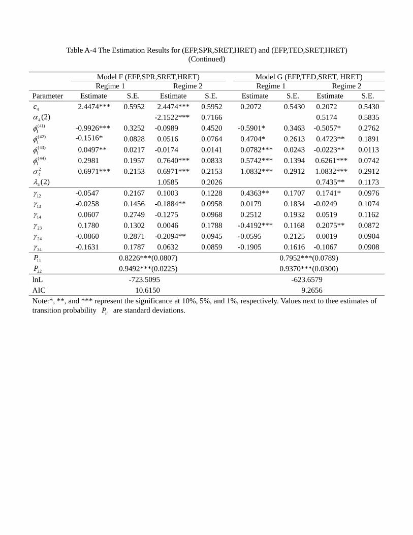
Table A-4 The Estimation Results for (EFP,SPR,SRET,HRET) and (EFP,TED,SRET,HRET) (Continued)

Model F (EFP,SPR,SRET,HRET) Model G (EFP,TED,SRET, HRET) Regime 1 Regime 2 Regime 1 Regime 2

Parameter Estimate S.E. Estimate S.E. Estimate S.E. Estimate S.E. 4c 2.4474*** 0.5952 2.4474*** 0.5952 0.2072 0.5430 0.2072 0.5430 4 (2) -2.1522*** 0.7166 0.5174 0.5835 (41)

1 -0.9926*** 0.3252 -0.0989 0.4520 -0.5901* 0.3463 -0.5057* 0.2762 (42)

1 -0.1516* 0.0828 0.0516 0.0764 0.4704* 0.2613 0.4723** 0.1891 (43)

1 0.0497** 0.0217 -0.0174 0.0141 0.0782*** 0.0243 -0.0223** 0.0113 (44)

1 0.2981 0.1957 0.7640*** 0.0833 0.5742*** 0.1394 0.6261*** 0.0742 24 0.6971*** 0.2153 0.6971*** 0.2153 1.0832*** 0.2912 1.0832*** 0.2912 4 (2) 1.0585 0.2026 0.7435** 0.1173

12 -0.0547 0.2167 0.1003 0.1228 0.4363** 0.1707 0.1741* 0.0976 13 -0.0258 0.1456 -0.1884** 0.0958 0.0179 0.1834 -0.0249 0.1074 14 0.0607 0.2749 -0.1275 0.0968 0.2512 0.1932 0.0519 0.1162 23 0.1780 0.1302 0.0046 0.1788 -0.4192*** 0.1168 0.2075** 0.0872 24 -0.0860 0.2871 -0.2094** 0.0945 -0.0595 0.2125 0.0019 0.0904 34 -0.1631 0.1787 0.0632 0.0859 -0.1905 0.1616 -0.1067 0.0908

11P 0.8226***(0.0807) 0.7952***(0.0789) 22P 0.9492***(0.0225) 0.9370***(0.0300)

lnL -723.5095 -623.6579 AIC 10.6150 9.2656 Note:*, **, and *** represent the significance at 10%, 5%, and 1%, respectively. Values next to thee estimates of transition probability iiP are standard deviations.

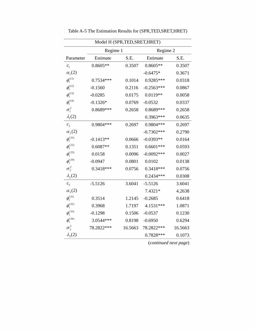
Table A-5 The Estimation Results for (SPR,TED,SRET,HRET)

Model H (SPR,TED,SRET,HRET) Regime 1 Regime 2

Parameter Estimate S.E. Estimate S.E.

1c 0.8605** 0.3507 0.8605** 0.3507

1(2) -0.6475* 0.3671 (11)

1 0.7534*** 0.1014 0.9285*** 0.0318 (12)

1 -0.1560 0.2116 -0.2563*** 0.0867 (13)

1 -0.0285 0.0175 0.0119** 0.0058 (14)

1 -0.1326* 0.0769 -0.0532 0.0337 21 0.8689*** 0.2658 0.8689*** 0.2658

1(2) 0.3963*** 0.0635

2c 0.9804*** 0.2697 0.9804*** 0.2697

2 (2) -0.7302*** 0.2790 (21)

1 -0.1413** 0.0666 -0.0393** 0.0164 (22)

1 0.6087** 0.1351 0.6601*** 0.0593 (23)

1 0.0158 0.0096 -0.0092*** 0.0027 (24)

1 -0.0947 0.0801 0.0102 0.0138 22 0.3418*** 0.0756 0.3418*** 0.0756

2 (2) 0.2434*** 0.0308

3c -5.5126 3.6041 -5.5126 3.6041

3(2) 7.4321* 4.2638 (31)

1 0.3514 1.2145 -0.2685 0.6418 (32)

1 0.3968 1.7197 4.1531*** 1.0871 (33)

1 -0.1298 0.1506 -0.0537 0.1230 (34)

1 3.0544*** 0.8198 -0.6950 0.6294 23 78.2822*** 16.5663 78.2822*** 16.5663

3(2) 0.7828*** 0.1073 (continued next page)

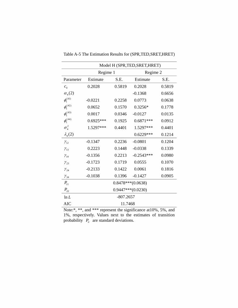
Table A-5 The Estimation Results for (SPR,TED,SRET,HRET)

Model H (SPR,TED,SRET,HRET) Regime 1 Regime 2 Parameter Estimate S.E. Estimate S.E.

4c 0.2028 0.5819 0.2028 0.5819

4 (2) -0.1368 0.6656 (41)

1 -0.0221 0.2258 0.0773 0.0638 (42)

1 0.0652 0.1570 0.3256* 0.1778 (43)

1 0.0017 0.0346 -0.0127 0.0135 (44)

1 0.6925*** 0.1925 0.6871*** 0.0912 24 1.5297*** 0.4401 1.5297*** 0.4401

4 (2) 0.6229*** 0.1214

12 -0.1347 0.2236 -0.0801 0.1204

13 0.2223 0.1448 -0.0338 0.1339

14 -0.1356 0.2213 -0.2543*** 0.0980

23 -0.1723 0.1719 0.0555 0.1070

24 -0.2133 0.1422 0.0061 0.1816

34 -0.1038 0.1396 -0.1427 0.0905

11P 0.8478***(0.0638)

22P 0.9447***(0.0230)

ln L -807.2657 AIC 11.7468 Note:*, **, and *** represent the significance at10%, 5%, and 1%, respectively. Values next to the estimates of transition probability iiP are standard deviations.

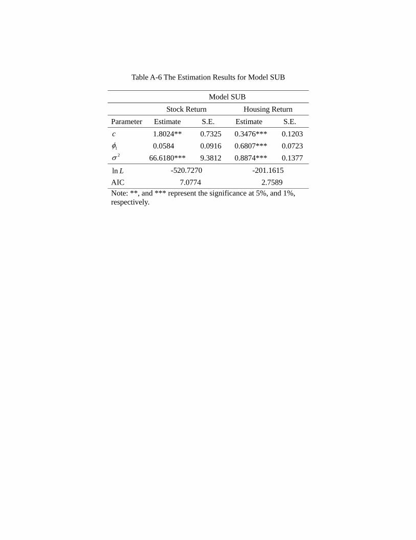
Table A-6 The Estimation Results for Model SUB

Model SUB Stock Return Housing Return Parameter Estimate S.E. Estimate S.E. c 1.8024** 0.7325 0.3476*** 0.1203

1 0.0584 0.0916 0.6807*** 0.0723 2 66.6180*** 9.3812 0.8874*** 0.1377

ln L -520.7270 -201.1615 AIC 7.0774 2.7589 Note: **, and *** represent the significance at 5%, and 1%, respectively.

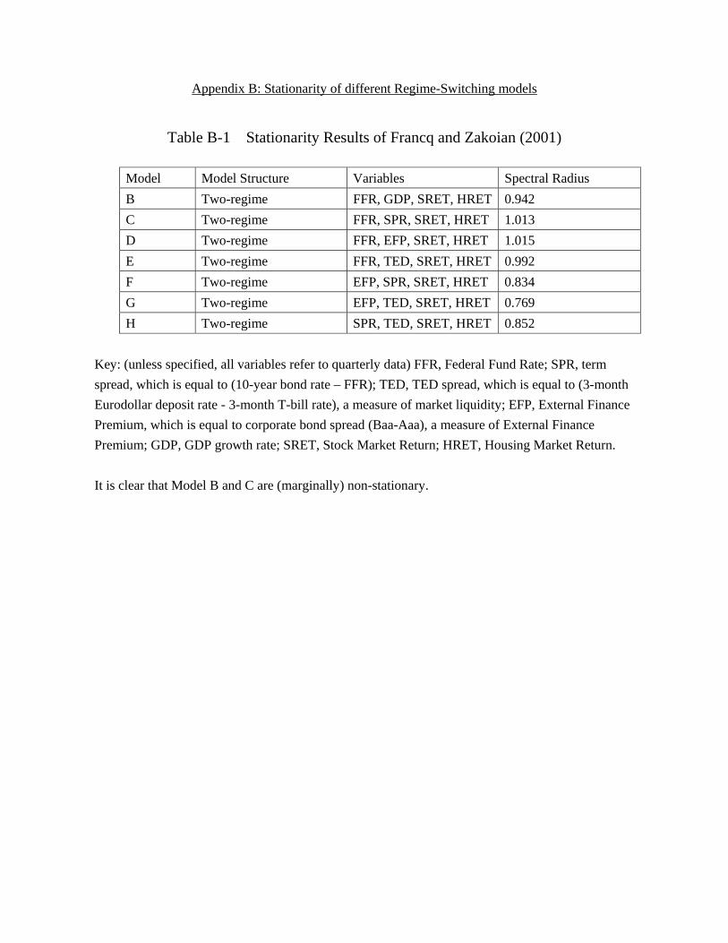
Appendix B: Stationarity of different Regime-Switching models

Table B-1 Stationarity Results of Francq and Zakoian (2001)

Model Model Structure Variables Spectral Radius B Two-regime FFR, GDP, SRET, HRET 0.942 C Two-regime FFR, SPR, SRET, HRET 1.013 D Two-regime FFR, EFP, SRET, HRET 1.015 E Two-regime FFR, TED, SRET, HRET 0.992 F Two-regime EFP, SPR, SRET, HRET 0.834 G Two-regime EFP, TED, SRET, HRET 0.769 H Two-regime SPR, TED, SRET, HRET 0.852

Key: (unless specified, all variables refer to quarterly data) FFR, Federal Fund Rate; SPR, term spread, which is equal to (10-year bond rate – FFR); TED, TED spread, which is equal to (3-month Eurodollar deposit rate - 3-month T-bill rate), a measure of market liquidity; EFP, External Finance Premium, which is equal to corporate bond spread (Baa-Aaa), a measure of External Finance Premium; GDP, GDP growth rate; SRET, Stock Market Return; HRET, Housing Market Return. It is clear that Model B and C are (marginally) non-stationary.

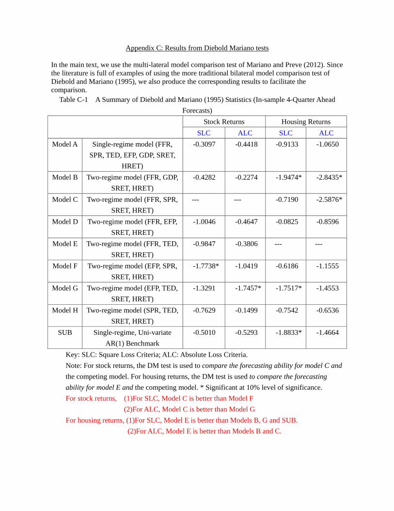
Appendix C: Results from Diebold Mariano tests In the main text, we use the multi-lateral model comparison test of Mariano and Preve (2012). Since the literature is full of examples of using the more traditional bilateral model comparison test of Diebold and Mariano (1995), we also produce the corresponding results to facilitate the comparison.

Table C-1 A Summary of Diebold and Mariano (1995) Statistics (In-sample 4-Quarter Ahead Forecasts)


Model A Single-regime model (FFR, SPR, TED, EFP, GDP, SRET,

HRET)

-0.3097 -0.4418 -0.9133 -1.0650

Model B Two-regime model (FFR, GDP, SRET, HRET)

-0.4282 -0.2274 -1.9474* -2.8435*

Model C Two-regime model (FFR, SPR, SRET, HRET)

--- --- -0.7190 -2.5876*

Model D Two-regime model (FFR, EFP, SRET, HRET)

-1.0046 -0.4647 -0.0825 -0.8596

Model E Two-regime model (FFR, TED, SRET, HRET)

-0.9847 -0.3806 --- ---

Model F Two-regime model (EFP, SPR, SRET, HRET)

-1.7738* -1.0419 -0.6186 -1.1555

Model G Two-regime model (EFP, TED, SRET, HRET)

-1.3291 -1.7457* -1.7517* -1.4553

Model H Two-regime model (SPR, TED, SRET, HRET)

-0.7629 -0.1499 -0.7542 -0.6536

SUB Single-regime, Uni-variate AR(1) Benchmark

-0.5010 -0.5293 -1.8833* -1.4664

Key: SLC: Square Loss Criteria; ALC: Absolute Loss Criteria. Note: For stock returns, the DM test is used to compare the forecasting ability for model C and the competing model. For housing returns, the DM test is used to compare the forecasting ability for model E and the competing model. * Significant at 10% level of significance. For stock returns, (1)For SLC, Model C is better than Model F

(2)For ALC, Model C is better than Model G For housing returns, (1)For SLC, Model E is better than Models B, G and SUB.

(2)For ALC, Model E is better than Models B and C.

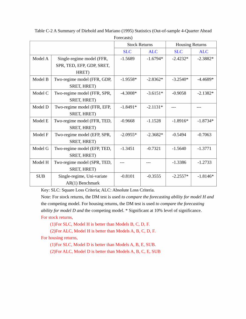
Table C-2 A Summary of Diebold and Mariano (1995) Statistics (Out-of-sample 4-Quarter Ahead Forecasts)


Model A Single-regime model (FFR, SPR, TED, EFP, GDP, SRET,

HRET)

-1.5689 -1.6794* -2.4232* -2.3882*

Model B Two-regime model (FFR, GDP, SRET, HRET)

-1.9558* -2.8362* -3.2540* -4.4689*

Model C Two-regime model (FFR, SPR, SRET, HRET)

-4.3008* -3.6151* -0.9058 -2.1382*

Model D Two-regime model (FFR, EFP, SRET, HRET)

-1.8491* -2.1131* --- ---

Model E Two-regime model (FFR, TED, SRET, HRET)

-0.9668 -1.1528 -1.8916* -1.8734*

Model F Two-regime model (EFP, SPR, SRET, HRET)

-2.0955* -2.3682* -0.5494 -0.7063

Model G Two-regime model (EFP, TED, SRET, HRET)

-1.3451 -0.7321 -1.5640 -1.3771

Model H Two-regime model (SPR, TED, SRET, HRET)

--- --- -1.3386 -1.2733

SUB Single-regime, Uni-variate AR(1) Benchmark

-0.8101 -0.3555 -2.2557* -1.8146*

Key: SLC: Square Loss Criteria; ALC: Absolute Loss Criteria. Note: For stock returns, the DM test is used to compare the forecasting ability for model H and the competing model. For housing returns, the DM test is used to compare the forecasting ability for model D and the competing model. * Significant at 10% level of significance. For stock returns,

(1)For SLC, Model H is better than Models B, C, D, F. (2)For ALC, Model H is better than Models A, B, C, D, F.

For housing returns, (1)For SLC, Model D is better than Models A, B, E, SUB. (2)For ALC, Model D is better than Models A, B, C, E, SUB

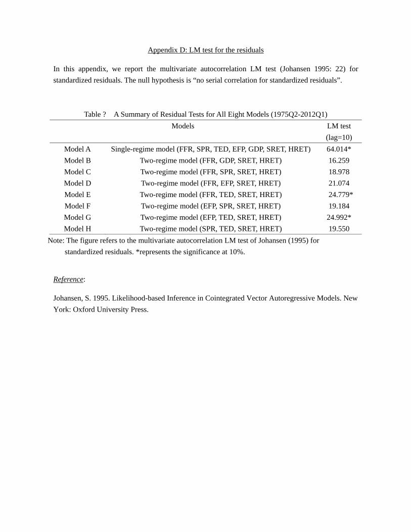
Appendix D: LM test for the residuals In this appendix, we report the multivariate autocorrelation LM test (Johansen 1995: 22) for standardized residuals. The null hypothesis is “no serial correlation for standardized residuals”.

Table ? A Summary of Residual Tests for All Eight Models (1975Q2-2012Q1) Models LM test

(lag=10) Model A Single-regime model (FFR, SPR, TED, EFP, GDP, SRET, HRET) 64.014* Model B Two-regime model (FFR, GDP, SRET, HRET) 16.259 Model C Two-regime model (FFR, SPR, SRET, HRET) 18.978 Model D Two-regime model (FFR, EFP, SRET, HRET) 21.074 Model E Two-regime model (FFR, TED, SRET, HRET) 24.779* Model F Two-regime model (EFP, SPR, SRET, HRET) 19.184 Model G Two-regime model (EFP, TED, SRET, HRET) 24.992* Model H Two-regime model (SPR, TED, SRET, HRET) 19.550

Note: The figure refers to the multivariate autocorrelation LM test of Johansen (1995) for standardized residuals. *represents the significance at 10%.

Reference: Johansen, S. 1995. Likelihood-based Inference in Cointegrated Vector Autoregressive Models. New York: Oxford University Press.

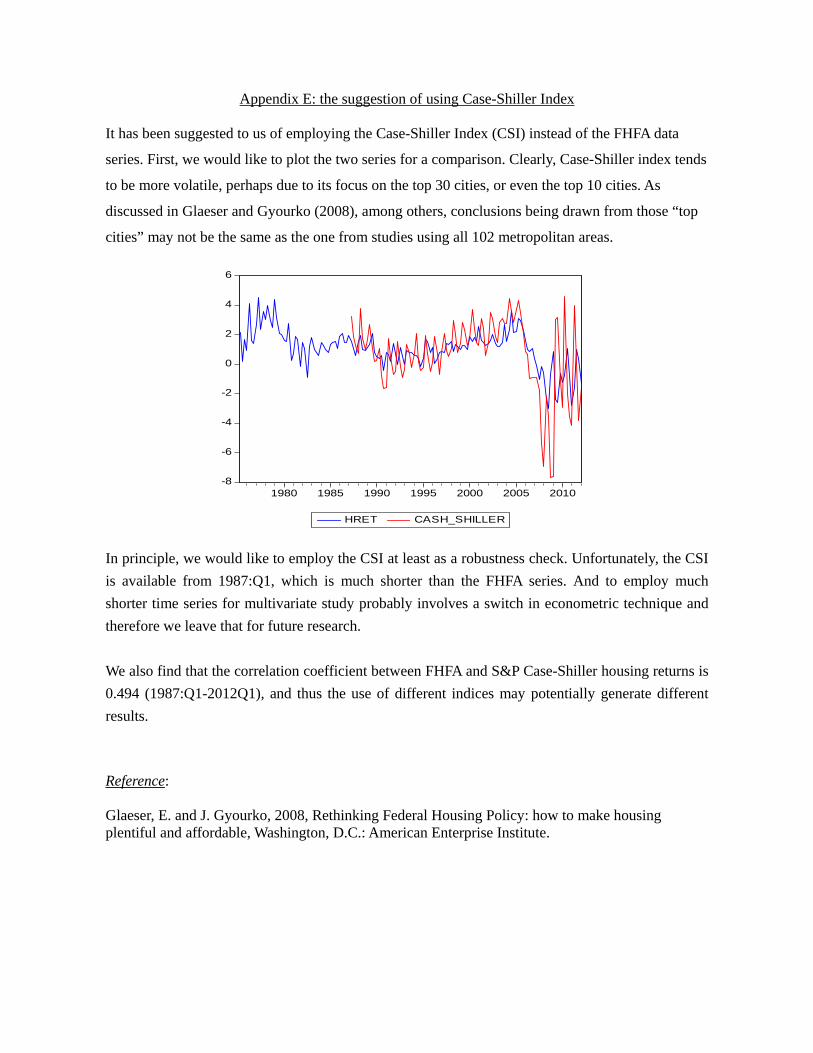
Appendix E: the suggestion of using Case-Shiller Index

It has been suggested to us of employing the Case-Shiller Index (CSI) instead of the FHFA data

series. First, we would like to plot the two series for a comparison. Clearly, Case-Shiller index tends

to be more volatile, perhaps due to its focus on the top 30 cities, or even the top 10 cities. As

discussed in Glaeser and Gyourko (2008), among others, conclusions being drawn from those “top

cities” may not be the same as the one from studies using all 102 metropolitan areas.

-8

-6

-4

-2

0

2

4

6

1980 1985 1990 1995 2000 2005 2010

HRET CASH_SHILLER

In principle, we would like to employ the CSI at least as a robustness check. Unfortunately, the CSI is available from 1987:Q1, which is much shorter than the FHFA series. And to employ much shorter time series for multivariate study probably involves a switch in econometric technique and therefore we leave that for future research. We also find that the correlation coefficient between FHFA and S&P Case-Shiller housing returns is 0.494 (1987:Q1-2012Q1), and thus the use of different indices may potentially generate different results. Reference: Glaeser, E. and J. Gyourko, 2008, Rethinking Federal Housing Policy: how to make housing plentiful and affordable, Washington, D.C.: American Enterprise Institute.

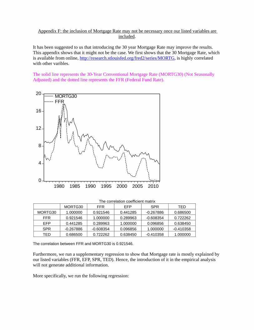
Appendix F: the inclusion of Mortgage Rate may not be necessary once our listed variables are included.

It has been suggested to us that introducing the 30 year Mortgage Rate may improve the results. This appendix shows that it might not be the case. We first shows that the 30 Mortgage Rate, which is available from online, http://research.stlouisfed.org/fred2/series/MORTG, is highly correlated with other varibles. The solid line represents the 30-Year Conventional Mortgage Rate (MORTG30) (Not Seasonally Adjusted) and the dotted line represents the FFR (Federal Fund Rate).

0

4

8

12

16

20

1980 1985 1990 1995 2000 2005 2010

MORTG30FFR

The correlation coefficient matrix MORTG30 FFR EFP SPR TED

MORTG30 1.000000 0.921546 0.441285 -0.267886 0.686500 FFR 0.921546 1.000000 0.289963 -0.608354 0.722262 EFP 0.441285 0.289963 1.000000 0.096856 0.638450 SPR -0.267886 -0.608354 0.096856 1.000000 -0.410358 TED 0.686500 0.722262 0.638450 -0.410358 1.000000

The correlation between FFR and MORTG30 is 0.921546. Furthermore, we run a supplementary regression to show that Mortgage rate is mostly explained by our listed variables (FFR, EFP, SPR, TED). Hence, the introduction of it in the empirical analysis will not generate additional information. More specifically, we run the following regression:

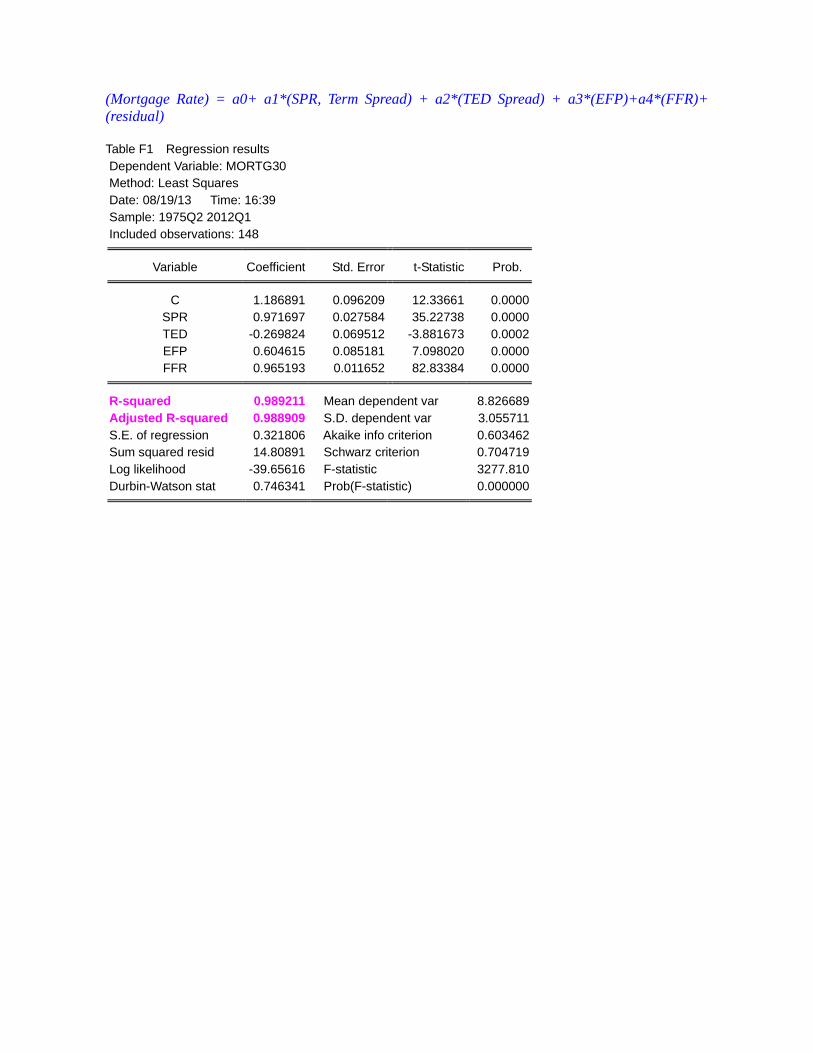
(Mortgage Rate) = a0+ a1*(SPR, Term Spread) + a2*(TED Spread) + a3*(EFP)+a4*(FFR)+ (residual) Table F1 Regression results Dependent Variable: MORTG30 Method: Least Squares Date: 08/19/13 Time: 16:39 Sample: 1975Q2 2012Q1 Included observations: 148

Variable Coefficient Std. Error t-Statistic Prob.

C 1.186891 0.096209 12.33661 0.0000SPR 0.971697 0.027584 35.22738 0.0000TED -0.269824 0.069512 -3.881673 0.0002EFP 0.604615 0.085181 7.098020 0.0000FFR 0.965193 0.011652 82.83384 0.0000

R-squared 0.989211 Mean dependent var 8.826689Adjusted R-squared 0.988909 S.D. dependent var 3.055711S.E. of regression 0.321806 Akaike info criterion 0.603462Sum squared resid 14.80891 Schwarz criterion 0.704719Log likelihood -39.65616 F-statistic 3277.810Durbin-Watson stat 0.746341 Prob(F-statistic) 0.000000

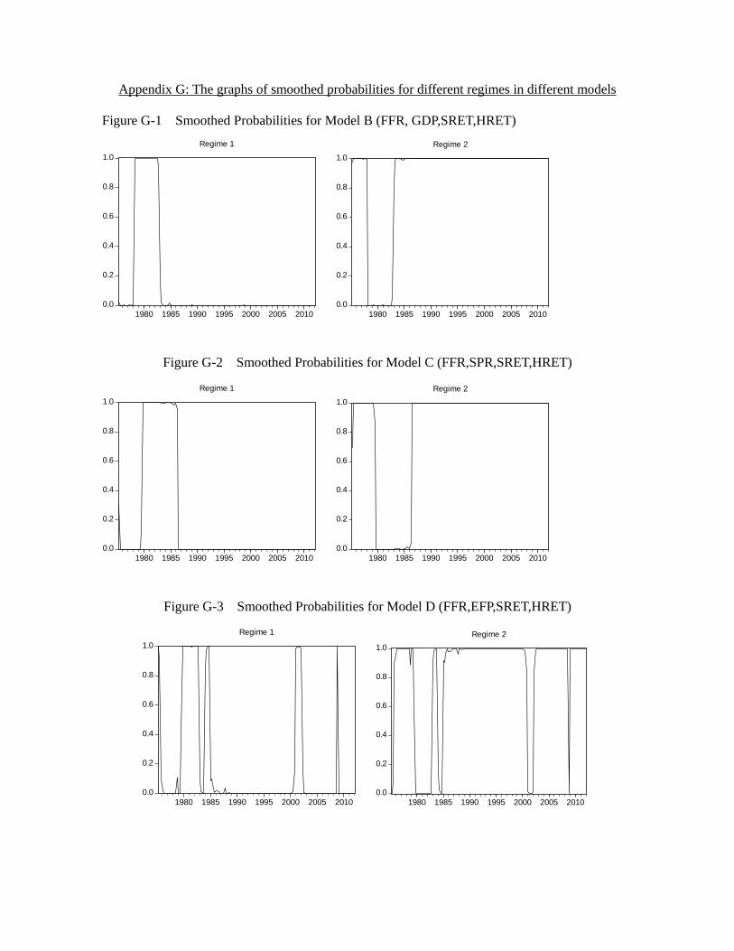
Appendix G: The graphs of smoothed probabilities for different regimes in different models Figure G-1 Smoothed Probabilities for Model B (FFR, GDP,SRET,HRET)

0.0

0.2

0.4

0.6

0.8

1.0

1980 1985 1990 1995 2000 2005 2010

Regime 1

0.0

0.2

0.4

0.6

0.8

1.0

1980 1985 1990 1995 2000 2005 2010

Regime 2

Figure G-2 Smoothed Probabilities for Model C (FFR,SPR,SRET,HRET)

0.0

0.2

0.4

0.6

0.8

1.0

1980 1985 1990 1995 2000 2005 2010

Regime 1

0.0

0.2

0.4

0.6

0.8

1.0

1980 1985 1990 1995 2000 2005 2010

Regime 2

Figure G-3 Smoothed Probabilities for Model D (FFR,EFP,SRET,HRET)

0.0

0.2

0.4

0.6

0.8

1.0

1980 1985 1990 1995 2000 2005 2010

Regime 1

0.0

0.2

0.4

0.6

0.8

1.0

1980 1985 1990 1995 2000 2005 2010

Regime 2

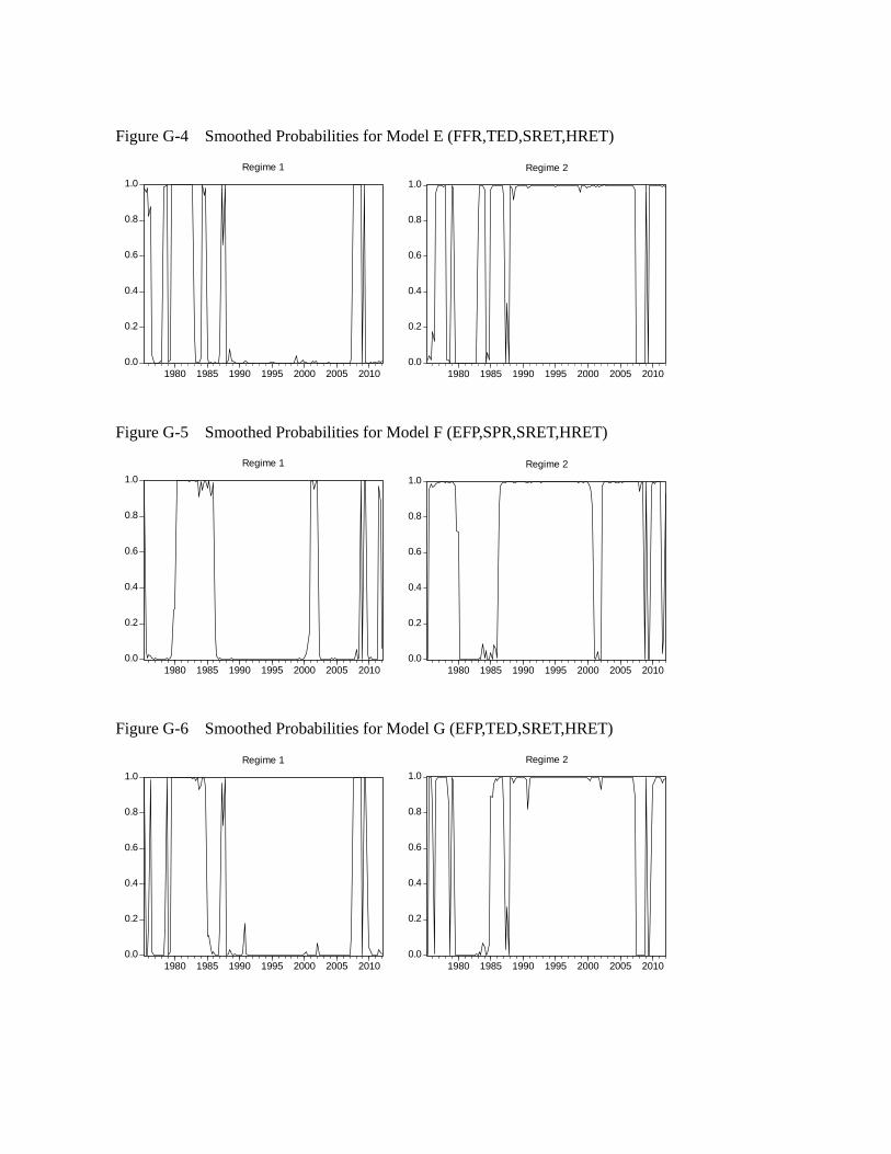
Figure G-4 Smoothed Probabilities for Model E (FFR,TED,SRET,HRET)

0.0

0.2

0.4

0.6

0.8

1.0

1980 1985 1990 1995 2000 2005 2010

Regime 1

0.0

0.2

0.4

0.6

0.8

1.0

1980 1985 1990 1995 2000 2005 2010

Regime 2

Figure G-5 Smoothed Probabilities for Model F (EFP,SPR,SRET,HRET)

0.0

0.2

0.4

0.6

0.8

1.0

1980 1985 1990 1995 2000 2005 2010

Regime 1

0.0

0.2

0.4

0.6

0.8

1.0

1980 1985 1990 1995 2000 2005 2010

Regime 2

Figure G-6 Smoothed Probabilities for Model G (EFP,TED,SRET,HRET)

0.0

0.2

0.4

0.6

0.8

1.0

1980 1985 1990 1995 2000 2005 2010

Regime 1

0.0

0.2

0.4

0.6

0.8

1.0

1980 1985 1990 1995 2000 2005 2010

Regime 2

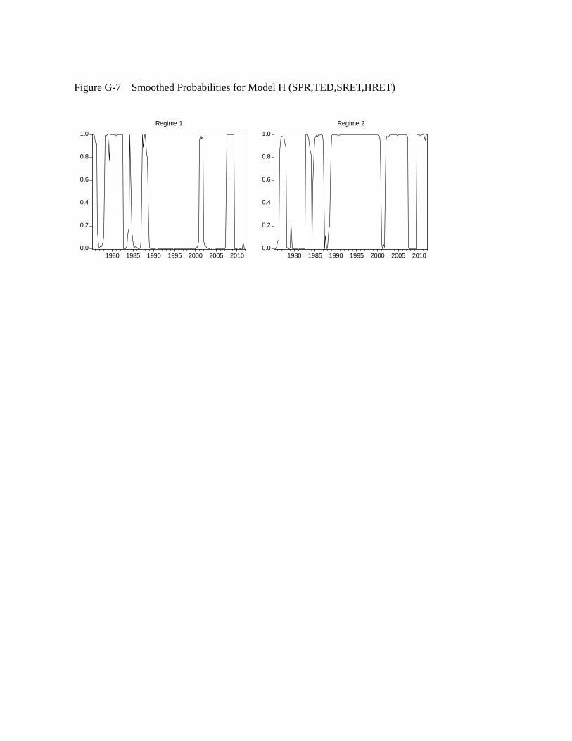
Figure G-7 Smoothed Probabilities for Model H (SPR,TED,SRET,HRET)

0.0

0.2

0.4

0.6

0.8

1.0

1980 1985 1990 1995 2000 2005 2010

Regime 1

0.0

0.2

0.4

0.6

0.8

1.0

1980 1985 1990 1995 2000 2005 2010

Regime 2

Appendix H: This appendix provides more details of the results which have been summarized in the text.

Table H-1. A Summary of Mariano and Preve (2011) Statistics for Stock Returns (In-sample 4-Quarter Ahead Forecasts)

Selected models S statistic cS statistic

Panel A: Squared loss criterion A, B, C, D, E, F, G, H, USB 7.2842 7.2230 Panel B: Absolute loss criterion A, B, C, D, E, F, G, H, USB 7.9727 7.9057 Note: The test statistics S and cS are used to compare the forecasting ability for various competing models. * Significant at 10% level of significance. Conclusion: All models have the same forecasting ability.

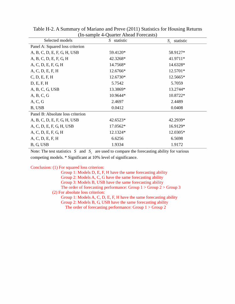
Table H-2. A Summary of Mariano and Preve (2011) Statistics for Housing Returns (In-sample 4-Quarter Ahead Forecasts)

Selected models S statistic cS statistic Panel A: Squared loss criterion A, B, C, D, E, F, G, H, USB 59.4120* 58.9127* A, B, C, D, E, F, G, H 42.3268* 41.9711* A, C, D, E, F, G, H 14.7568* 14.6328* A, C, D, E, F, H 12.6766* 12.5701* C, D, E, F, H 12.6730* 12.5665* D, E, F, H 5.7542 5.7059 A, B, C, G, USB 13.3869* 13.2744* A, B, C, G 10.9644* 10.8722* A, C, G 2.4697 2.4489 B, USB 0.0412 0.0408 Panel B: Absolute loss criterion A, B, C, D, E, F, G, H, USB 42.6523* 42.2939* A, C, D, E, F, G, H, USB 17.0562* 16.9129* A, C, D, E, F, G, H 12.1324* 12.0305* A, C, D, E, F, H 6.6256 6.5698 B, G, USB 1.9334 1.9172 Note: The test statistics S and cS are used to compare the forecasting ability for various competing models. * Significant at 10% level of significance. Conclusion: (1) For squared loss criterion:

Group 1: Models D, E, F, H have the same forecasting ability Group 2: Models A, C, G have the same forecasting ability Group 3: Models B, USB have the same forecasting ability The order of forecasting performance: Group 1 > Group 2 > Group 3

(2) For absolute loss criterion: Group 1: Models A, C, D, E, F, H have the same forecasting ability Group 2: Models B, G, USB have the same forecasting ability

The order of forecasting performance: Group 1 > Group 2

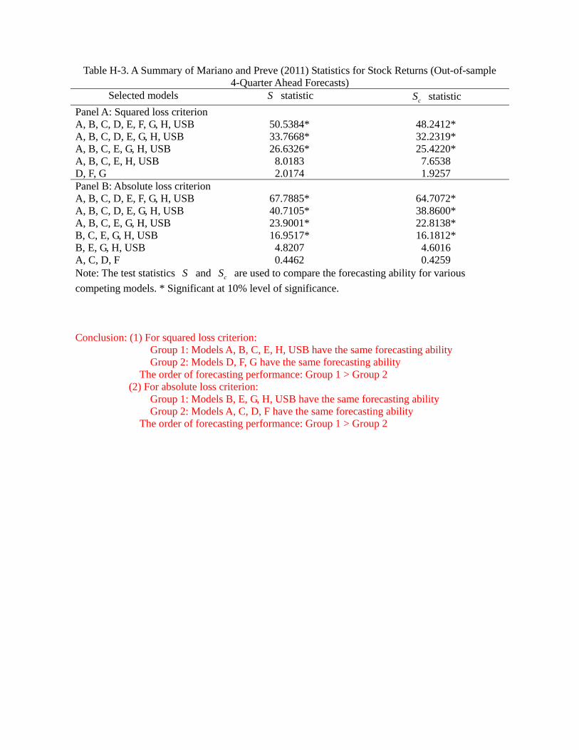
Table H-3. A Summary of Mariano and Preve (2011) Statistics for Stock Returns (Out-of-sample 4-Quarter Ahead Forecasts)

Selected models S statistic cS statistic Panel A: Squared loss criterion A, B, C, D, E, F, G, H, USB 50.5384* 48.2412* A, B, C, D, E, G, H, USB 33.7668* 32.2319* A, B, C, E, G, H, USB 26.6326* 25.4220* A, B, C, E, H, USB 8.0183 7.6538 D, F, G 2.0174 1.9257 Panel B: Absolute loss criterion A, B, C, D, E, F, G, H, USB 67.7885* 64.7072* A, B, C, D, E, G, H, USB 40.7105* 38.8600* A, B, C, E, G, H, USB 23.9001* 22.8138* B, C, E, G, H, USB 16.9517* 16.1812* B, E, G, H, USB 4.8207 4.6016 A, C, D, F 0.4462 0.4259 Note: The test statistics S and cS are used to compare the forecasting ability for various competing models. * Significant at 10% level of significance. Conclusion: (1) For squared loss criterion:

Group 1: Models A, B, C, E, H, USB have the same forecasting ability Group 2: Models D, F, G have the same forecasting ability The order of forecasting performance: Group 1 > Group 2

(2) For absolute loss criterion: Group 1: Models B, E, G, H, USB have the same forecasting ability

Group 2: Models A, C, D, F have the same forecasting ability The order of forecasting performance: Group 1 > Group 2

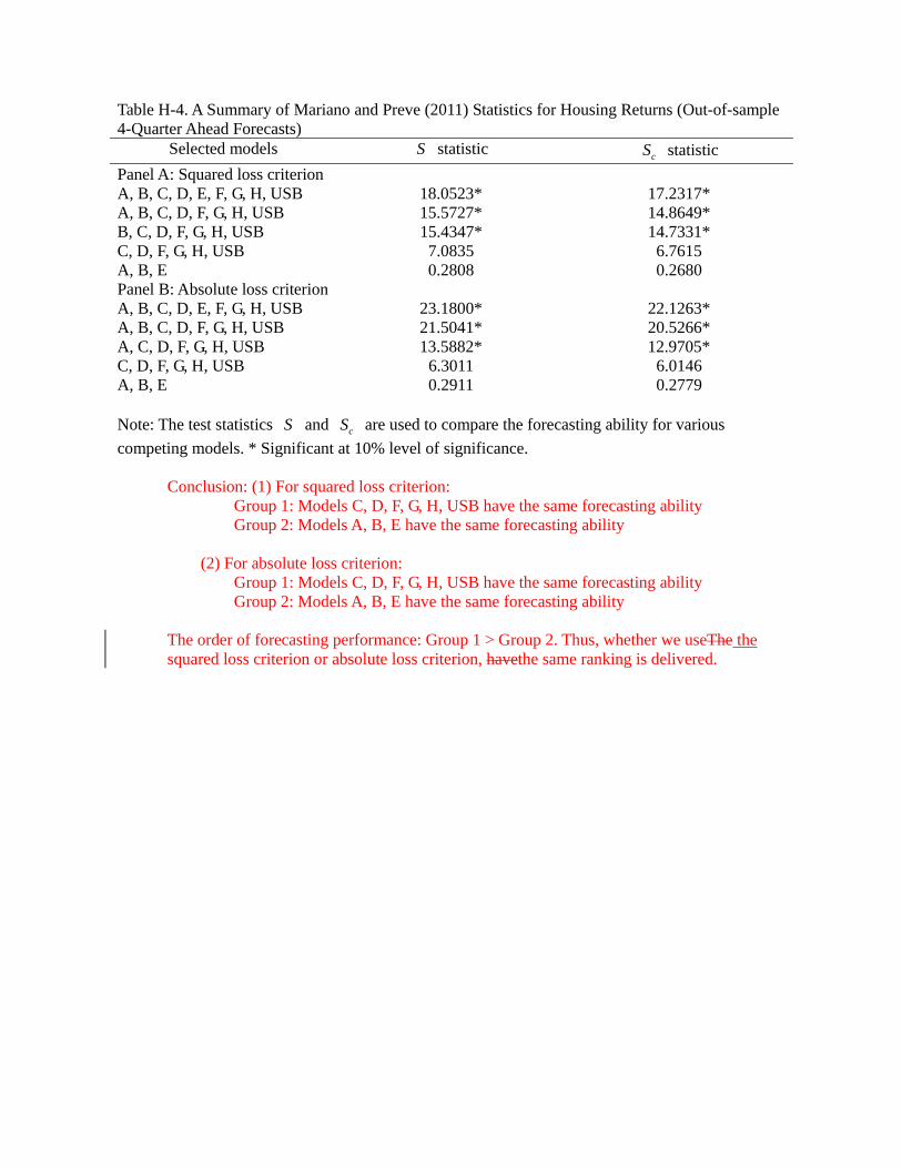
Table H-4. A Summary of Mariano and Preve (2011) Statistics for Housing Returns (Out-of-sample 4-Quarter Ahead Forecasts)

Selected models S statistic cS statistic Panel A: Squared loss criterion A, B, C, D, E, F, G, H, USB 18.0523* 17.2317* A, B, C, D, F, G, H, USB 15.5727* 14.8649* B, C, D, F, G, H, USB 15.4347* 14.7331* C, D, F, G, H, USB 7.0835 6.7615 A, B, E 0.2808 0.2680 Panel B: Absolute loss criterion A, B, C, D, E, F, G, H, USB 23.1800* 22.1263* A, B, C, D, F, G, H, USB 21.5041* 20.5266* A, C, D, F, G, H, USB 13.5882* 12.9705* C, D, F, G, H, USB 6.3011 6.0146 A, B, E 0.2911 0.2779 Note: The test statistics S and cS are used to compare the forecasting ability for various competing models. * Significant at 10% level of significance.

Conclusion: (1) For squared loss criterion: Group 1: Models C, D, F, G, H, USB have the same forecasting ability

Group 2: Models A, B, E have the same forecasting ability

(2) For absolute loss criterion: Group 1: Models C, D, F, G, H, USB have the same forecasting ability

Group 2: Models A, B, E have the same forecasting ability The order of forecasting performance: Group 1 > Group 2. Thus, whether we useThe the squared loss criterion or absolute loss criterion, havethe same ranking is delivered.

Appendix I: This appendix provides a simple review of the literature which chooses a similar boom-bust date as we do. AS it can be expected, the dating of bust regime varies across research papers, reflecting the difference in modelling techniques as well as research focuses. Nevertheless, there seems to be a collection of studies which also select the beginning of 2006 as the start of bust phase of the cycle. 1. Huang (2014) extends Galvão’s (2006) SBTVAR framework and shows that a persistent

housing-bust phase in US begins in March 2006. This finding is in line with prior studies that identify 2006 as the starting period of the recent housing bust in the U.S.

2. Ferreira, Gyourko, and Tracy (2010) point out that loan-to-value ratios of some local housing markets are higher than 85% in 2006, and specify that the housing bust starts in 2006.

3. Huang and Tang (2012) argue that tight housing supply constraints, which result in supply inelasticity, magnify the recent housing price bust since 2006.

4. In’t-Veld, Raciborski, Ratto, and Roeger (2011) propose that the decline in residential investment since the early-2006 led to the economic recession, and identify the bust of the housing bubble in 2006.

5. Khandani, Lo, and Merton (2013) estimate the potential losses of the US housing market due to a housing price bust from 2006.

6. Lutz, Molloy, and Shan (2011) address five channels through which the US housing market influences state and local tax revenues. They provide estimates of a fall in sales tax revenue from 2006 to 2009 and find that housing prices peak in the first quarter of 2006, followed by a collapse of housing price growths.

7. Nichols, Oliner, and Mulhall (2013) show that residential and commercial land price indexes plunge after peaking in 2006.

8. Chen et al. (2014): According to FHFA house price index, the U.S. average house price has grown consecutively around 1.6% for the period 1995Q4 – 2005Q4, reaching a total of 89% in capital gains. The returns on housing started to decline around 2006q1 and then precipitated in the following quarters when the subprime mortgage problem aggravated. Using RW model, they identify the boom-bust regime capturing the periods where housing returns exhibited high volatility before mid-1980s and after 2005q4.

9. Kouwenberg and Zwinkels (2014): The real house price index reached a maximum in the first quarter of 2006, when it was 48% higher than the fundamental value estimate, and the prolonged period of overvaluation ended in the first quarter of 2009, as the price eventually dropped below the fundamental value.

10. Cetorelli and Goldberg (2012) show that internal capital markets of global banks also contribute to the international propagation of shocks. Using balance sheets data for chartered US banks over the period 1980-2009, the sample is split over two samples, a pre-crisis period using quarterly data on individual banks from “Call reports” from 1980Q1 to 2005Q4, and a crisis period sample using weekly series on aggregate Assets and Liabilities of Commercial Banks in the United States (Fed. H.8 Statistical Release).

11. Cetorelli and Goldberg (2010) confirm that global banks played a significant role in the crisis transmission to emerging market economies. Using banking statistics data from the BIS and IMF’s International Financial Statistics for 17 source countries from the OECD and 94 destination countries from emerging Europe, Asia, and Latin from 2006 to 2009 they examine the relationships between adverse liquidity shocks on main developed-country banking systems to emerging markets, isolating loan supply from loan demand effects. The sample is split in to a pre-crisis period from 2006Q2 to 2007Q2 and a post-crisis period from 2008Q3 to 2009Q2,

leaving out the crisis event period between 2007Q3 and 2008Q2 when market functioning was disrupted by the Lehman shock. Alternative datings were considered in robustness tests.

12. Bertay and Gong (2014) use an international panel to analyze the relationship between securitization and macroeconomic performance. Our findings suggest that economic growth is negatively related to country-level securitization activities, even before the 2007-2009 financial crisis. The annual sample is split into 1995-2006 and 2006-2012.

13. Shiller (2007): Between the bottom in the 4th quarter of 1996 and the peak in the first quarter of 2006, real home prices rose 86% nationally in the United States.

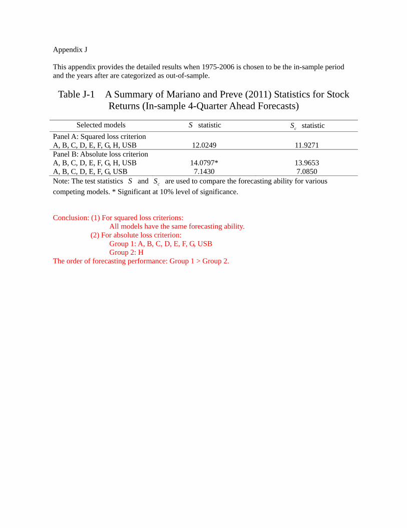
Appendix J This appendix provides the detailed results when 1975-2006 is chosen to be the in-sample period and the years after are categorized as out-of-sample.

Table J-1 A Summary of Mariano and Preve (2011) Statistics for Stock Returns (In-sample 4-Quarter Ahead Forecasts)


Panel A: Squared loss criterion A, B, C, D, E, F, G, H, USB 12.0249 11.9271 Panel B: Absolute loss criterion A, B, C, D, E, F, G, H, USB 14.0797* 13.9653 A, B, C, D, E, F, G, USB 7.1430 7.0850 Note: The test statistics S and cS are used to compare the forecasting ability for various competing models. * Significant at 10% level of significance.

Conclusion: (1) For squared loss criterions:

All models have the same forecasting ability. (2) For absolute loss criterion:

Group 1: A, B, C, D, E, F, G, USB Group 2: H The order of forecasting performance: Group 1 > Group 2.

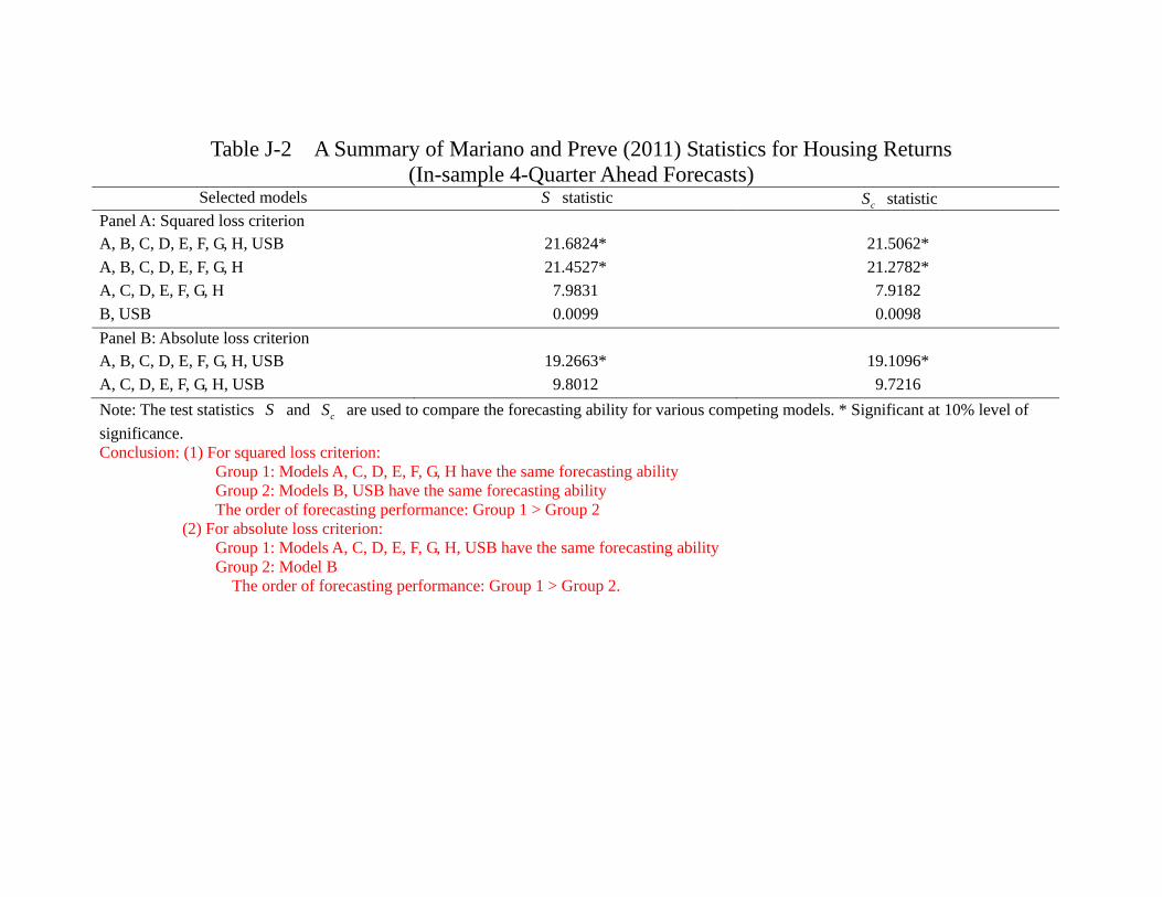
Table J-2 A Summary of Mariano and Preve (2011) Statistics for Housing Returns

(In-sample 4-Quarter Ahead Forecasts) Selected models S statistic cS statistic

Panel A: Squared loss criterion A, B, C, D, E, F, G, H, USB 21.6824* 21.5062* A, B, C, D, E, F, G, H 21.4527* 21.2782* A, C, D, E, F, G, H 7.9831 7.9182 B, USB 0.0099 0.0098 Panel B: Absolute loss criterion A, B, C, D, E, F, G, H, USB 19.2663* 19.1096* A, C, D, E, F, G, H, USB 9.8012 9.7216 Note: The test statistics S and cS are used to compare the forecasting ability for various competing models. * Significant at 10% level of significance. Conclusion: (1) For squared loss criterion:

Group 1: Models A, C, D, E, F, G, H have the same forecasting ability Group 2: Models B, USB have the same forecasting ability The order of forecasting performance: Group 1 > Group 2

(2) For absolute loss criterion: Group 1: Models A, C, D, E, F, G, H, USB have the same forecasting ability Group 2: Model B

The order of forecasting performance: Group 1 > Group 2.

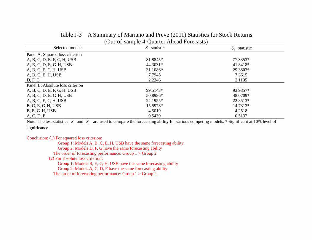
Table J-3 A Summary of Mariano and Preve (2011) Statistics for Stock Returns (Out-of-sample 4-Quarter Ahead Forecasts)

Selected models S statistic cS statistic Panel A: Squared loss criterion A, B, C, D, E, F, G, H, USB 81.8845* 77.3353* A, B, C, D, E, G, H, USB 44.3031* 41.8418* A, B, C, E, G, H, USB 31.1086* 29.3803* A, B, C, E, H, USB 7.7945 7.3615 D, F, G 2.2346 2.1105 Panel B: Absolute loss criterion A, B, C, D, E, F, G, H, USB 99.5143* 93.9857* A, B, C, D, E, G, H, USB 50.8986* 48.0709* A, B, C, E, G, H, USB 24.1955* 22.8513* B, C, E, G, H, USB 15.5978* 14.7313* B, E, G, H, USB 4.5019 4.2518 A, C, D, F 0.5439 0.5137 Note: The test statistics S and cS are used to compare the forecasting ability for various competing models. * Significant at 10% level of significance. Conclusion: (1) For squared loss criterion:

Group 1: Models A, B, C, E, H, USB have the same forecasting ability Group 2: Models D, F, G have the same forecasting ability The order of forecasting performance: Group 1 > Group 2


Group 2: Models A, C, D, F have the same forecasting ability The order of forecasting performance: Group 1 > Group 2.

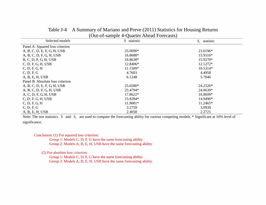
Table J-4 A Summary of Mariano and Preve (2011) Statistics for Housing Returns (Out-of-sample 4-Quarter Ahead Forecasts)

Selected models S statistic cS statistic Panel A: Squared loss criterion A, B, C, D, E, F, G, H, USB 25.0090* 23.6196* A, B, C, D, F, G, H, USB 16.8688* 15.9316* B, C, D, F, G, H, USB 16.8638* 15.9270* C, D, F, G, H, USB 12.8406* 12.1272* C, D, F, G, H 11.1509* 10.5314* C, D, F, G 4.7603 4.4958 A, B, E, H, USB 6.1248 5.7846 Panel B: Absolute loss criterion A, B, C, D, E, F, G, H, USB 25.6580* 24.2326* A, B, C, D, F, G, H, USB 25.4794* 24.0639* A, C, D, F, G, H, USB 17.8622* 16.8699* C, D, F, G, H, USB 15.8284* 14.9490* C, D, F, G, H 11.9081* 11.2465* C, D, F, G 3.2759 3.0939 A, B, E, H, USB 2.4058 2.2721 Note: The test statistics S and cS are used to compare the forecasting ability for various competing models. * Significant at 10% level of significance.

Conclusion: (1) For squared loss criterion: Group 1: Models C, D, F, G have the same forecasting ability

Group 2: Models A, B, E, H, USB have the same forecasting ability

(2) For absolute loss criterion: Group 1: Models C, D, F, G have the same forecasting ability

Group 2: Models A, B, E, H, USB have the same forecasting ability.

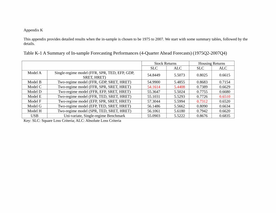
Appendix K This appendix provides detailed results when the in-sample is chosen to be 1975 to 2007. We start with some summary tables, followed by the details. Table K-1 A Summary of In-sample Forecasting Performances (4-Quarter Ahead Forecasts) (1975Q2-2007Q4)


Model A Single-regime model (FFR, SPR, TED, EFP, GDP, SRET, HRET) 54.8449 5.5073 0.8025 0.6615


USB Uni-variate, Single-regime Benchmark 55.0903 5.5222 0.8676 0.6835 Key: SLC: Square Loss Criteria; ALC: Absolute Loss Criteria

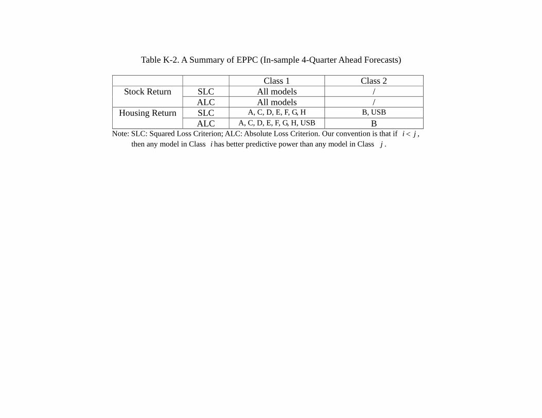
Table K-2. A Summary of EPPC (In-sample 4-Quarter Ahead Forecasts)

Class 1 Class 2 Stock Return SLC All models /

ALC All models / Housing Return SLC A, C, D, E, F, G, H B, USB

ALC A, C, D, E, F, G, H, USB B Note: SLC: Squared Loss Criterion; ALC: Absolute Loss Criterion. Our convention is that if i j ,

then any model in Class i has better predictive power than any model in Class j .

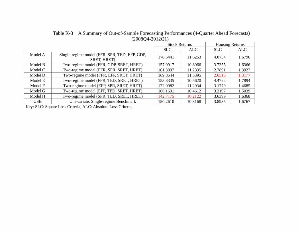
Table K-3 A Summary of Out-of-Sample Forecasting Performances (4-Quarter Ahead Forecasts) (2008Q4-2012Q1)





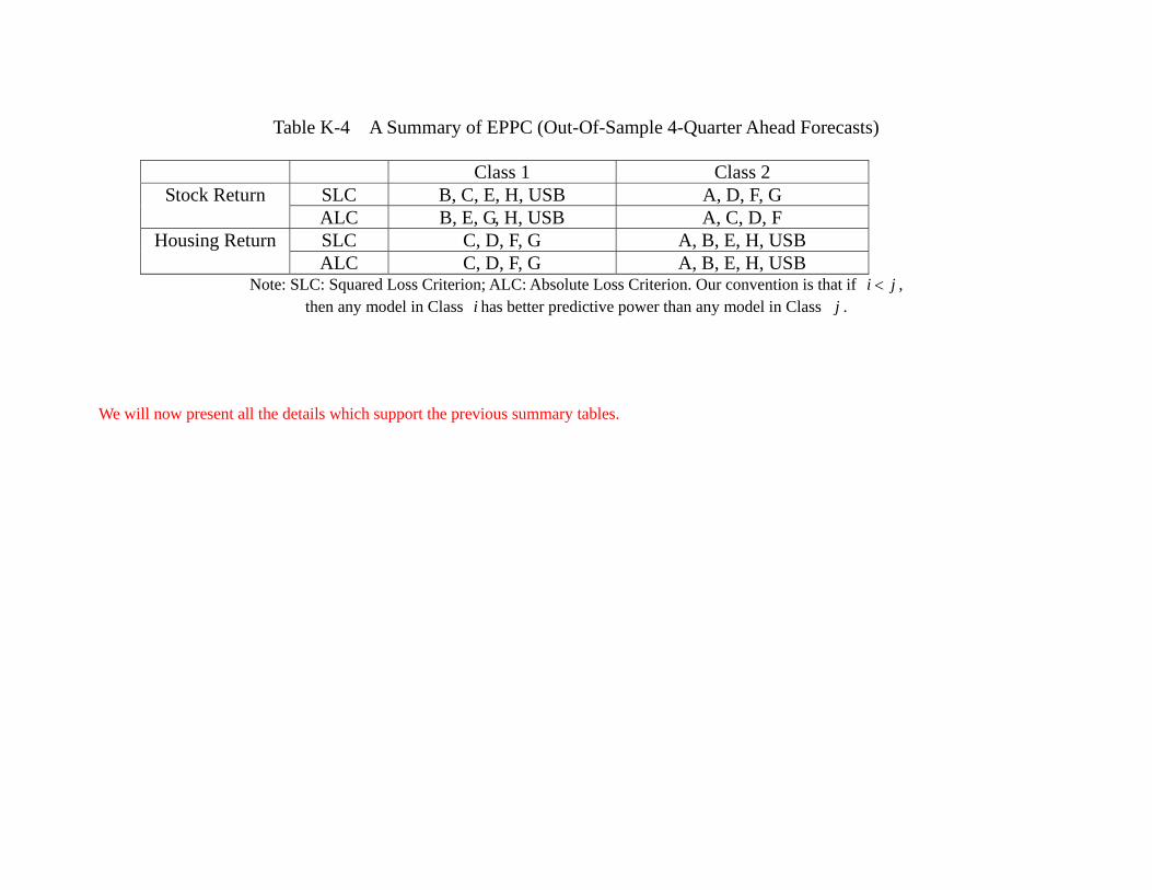
Table K-4 A Summary of EPPC (Out-Of-Sample 4-Quarter Ahead Forecasts)

Class 1 Class 2 Stock Return SLC B, C, E, H, USB A, D, F, G

ALC B, E, G, H, USB A, C, D, F Housing Return SLC C, D, F, G A, B, E, H, USB

ALC C, D, F, G A, B, E, H, USB Note: SLC: Squared Loss Criterion; ALC: Absolute Loss Criterion. Our convention is that if i j ,

then any model in Class i has better predictive power than any model in Class j .

We will now present all the details which support the previous summary tables.

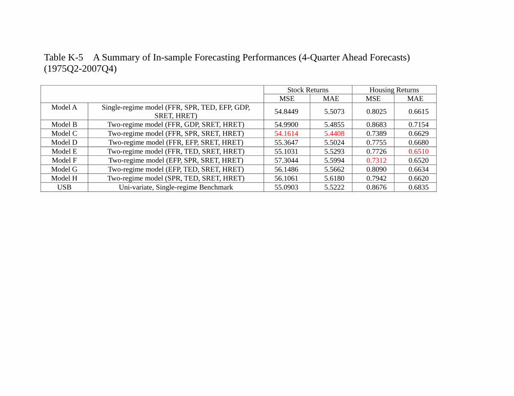
Table K-5 A Summary of In-sample Forecasting Performances (4-Quarter Ahead Forecasts) (1975Q2-2007Q4)

Stock Returns Housing Returns

MSE MAE MSE MAE Model A Single-regime model (FFR, SPR, TED, EFP, GDP,

SRET, HRET) 54.8449 5.5073 0.8025 0.6615


USB Uni-variate, Single-regime Benchmark 55.0903 5.5222 0.8676 0.6835

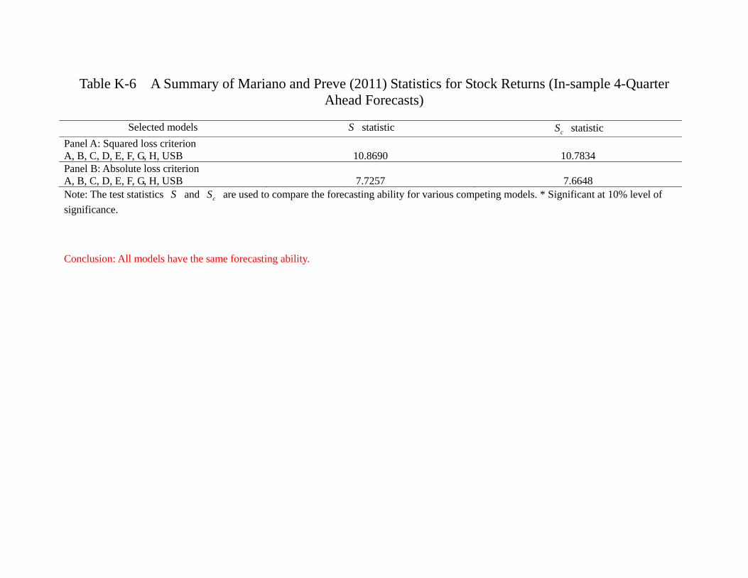
Table K-6 A Summary of Mariano and Preve (2011) Statistics for Stock Returns (In-sample 4-Quarter Ahead Forecasts)


Panel A: Squared loss criterion A, B, C, D, E, F, G, H, USB 10.8690 10.7834 Panel B: Absolute loss criterion A, B, C, D, E, F, G, H, USB 7.7257 7.6648 Note: The test statistics S and cS are used to compare the forecasting ability for various competing models. * Significant at 10% level of significance.

Conclusion: All models have the same forecasting ability.

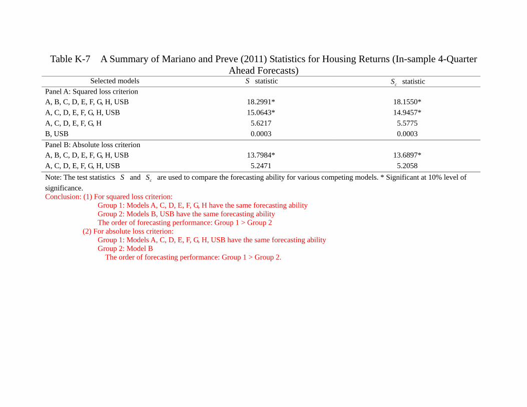
Table K-7 A Summary of Mariano and Preve (2011) Statistics for Housing Returns (In-sample 4-Quarter Ahead Forecasts)

Selected models S statistic cS statistic Panel A: Squared loss criterion A, B, C, D, E, F, G, H, USB 18.2991* 18.1550* A, C, D, E, F, G, H, USB 15.0643* 14.9457* A, C, D, E, F, G, H 5.6217 5.5775 B, USB 0.0003 0.0003 Panel B: Absolute loss criterion A, B, C, D, E, F, G, H, USB 13.7984* 13.6897* A, C, D, E, F, G, H, USB 5.2471 5.2058 Note: The test statistics S and cS are used to compare the forecasting ability for various competing models. * Significant at 10% level of significance. Conclusion: (1) For squared loss criterion:

Group 1: Models A, C, D, E, F, G, H have the same forecasting ability Group 2: Models B, USB have the same forecasting ability The order of forecasting performance: Group 1 > Group 2

(2) For absolute loss criterion: Group 1: Models A, C, D, E, F, G, H, USB have the same forecasting ability Group 2: Model B

The order of forecasting performance: Group 1 > Group 2.

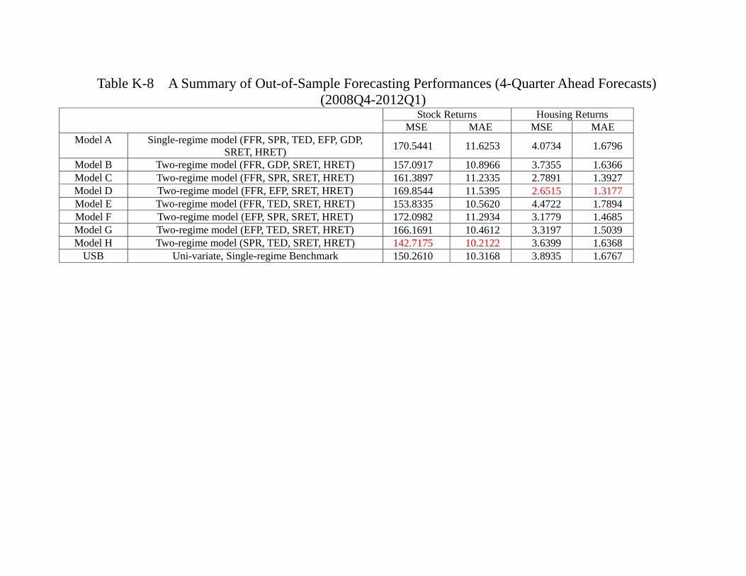
Table K-8 A Summary of Out-of-Sample Forecasting Performances (4-Quarter Ahead Forecasts) (2008Q4-2012Q1)

Stock Returns Housing Returns MSE MAE MSE MAE



USB Uni-variate, Single-regime Benchmark 150.2610 10.3168 3.8935 1.6767

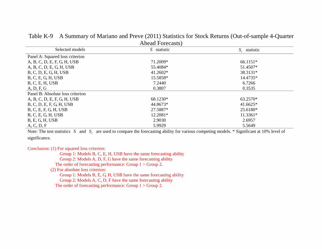
Table K-9 A Summary of Mariano and Preve (2011) Statistics for Stock Returns (Out-of-sample 4-Quarter Ahead Forecasts)

Selected models S statistic cS statistic Panel A: Squared loss criterion A, B, C, D, E, F, G, H, USB 71.2009* 66.1151* A, B, C, D, E, G, H, USB 55.4084* 51.4507* B, C, D, E, G, H, USB 41.2602* 38.3131* B, C, E, G, H, USB 15.5858* 14.4735* B, C, E, H, USB 7.2440 6.7266 A, D, F, G 0.3807 0.3535 Panel B: Absolute loss criterion A, B, C, D, E, F, G, H, USB 68.1230* 63.2570* B, C, D, E, F, G, H, USB 44.8673* 41.6625* B, C, E, F, G, H, USB 27.5887* 25.6180* B, C, E, G, H, USB 12.2081* 11.3361* B, E, G, H, USB 2.9030 2.6957 A, C, D, F 5.9929 5.5649 Note: The test statistics S and cS are used to compare the forecasting ability for various competing models. * Significant at 10% level of significance. Conclusion: (1) For squared loss criterion:

Group 1: Models B, C, E, H, USB have the same forecasting ability Group 2: Models A, D, F, G have the same forecasting ability The order of forecasting performance: Group 1 > Group 2.


Group 2: Models A, C, D, F have the same forecasting ability The order of forecasting performance: Group 1 > Group 2.

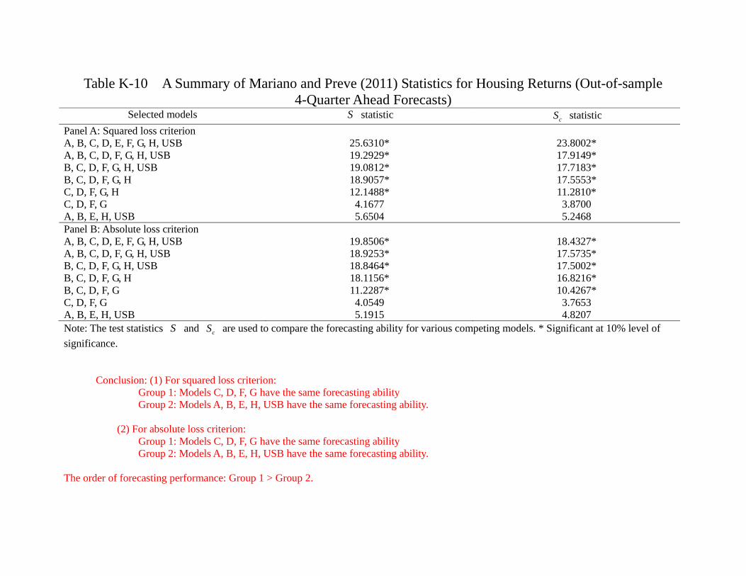
Table K-10 A Summary of Mariano and Preve (2011) Statistics for Housing Returns (Out-of-sample 4-Quarter Ahead Forecasts)

Selected models S statistic cS statistic Panel A: Squared loss criterion A, B, C, D, E, F, G, H, USB 25.6310* 23.8002* A, B, C, D, F, G, H, USB 19.2929* 17.9149* B, C, D, F, G, H, USB 19.0812* 17.7183* B, C, D, F, G, H 18.9057* 17.5553* C, D, F, G, H 12.1488* 11.2810* C, D, F, G 4.1677 3.8700 A, B, E, H, USB 5.6504 5.2468 Panel B: Absolute loss criterion A, B, C, D, E, F, G, H, USB 19.8506* 18.4327* A, B, C, D, F, G, H, USB 18.9253* 17.5735* B, C, D, F, G, H, USB 18.8464* 17.5002* B, C, D, F, G, H 18.1156* 16.8216* B, C, D, F, G 11.2287* 10.4267* C, D, F, G 4.0549 3.7653 A, B, E, H, USB 5.1915 4.8207 Note: The test statistics S and cS are used to compare the forecasting ability for various competing models. * Significant at 10% level of significance.

Conclusion: (1) For squared loss criterion:

Group 1: Models C, D, F, G have the same forecasting ability Group 2: Models A, B, E, H, USB have the same forecasting ability.

(2) For absolute loss criterion: Group 1: Models C, D, F, G have the same forecasting ability

Group 2: Models A, B, E, H, USB have the same forecasting ability. The order of forecasting performance: Group 1 > Group 2.

Documents

LOSING TRACK OF THE ASSET MARKETS: THE CASE OF HOUSING … · LOSING TRACK OF THE ASSET MARKETS: THE CASE OF HOUSING AND STOCK ... Carl Hempel, 1942, The Function of General Laws