1

Long-term Estimates of U.S. Productivity and Growth

by

Dale W. Jorgenson, Harvard University,

Mun S. Ho, Harvard University,

and

Jon D. Samuels, Bureau of Economic Analysis1

May 12, 2014

Prepared for Presentation at Third World KLEMS Conference Growth and Stagnation in the World Economy Tokyo, May 19-20, 2014

1The views expressed in this paper are solely those of the authors and not necessarily those of the U.S. Bureau of Economic Analysis or the U.S. Department of Commerce.

2

1. Introduction

The objective of this paper is to provide a new historical perspective on postwar US

economic growth. For this purpose we have constructed a data set on the growth of output and

productivity by industry for the period 1947-2010. This covers 65 industries and uses the North

American Industry Classification System (NAICS). We incorporate output for each industry as well

as inputs of capital (K), labor (L), energy (E), materials (M), and services (S). We describe the

postwar evolution in the primary factors of production, capital and labor services, in greater detail.

Productivity is the ratio of output to input.

Productivity growth is the key economic indicator of innovation. Economic growth can take

place without innovation through replication of established technologies. Investment increases the

availability of these technologies, while the labor force expands as population grows. With only

replication and without innovation, output will increase in proportion to capital and labor inputs. By

contrast the successful introduction of new products and new or altered processes, organization

structures, systems, and business models generates growth of output that exceeds the growth of

capital and labor inputs. This results in growth in productivity or output per unit of input.

We show that the great preponderance of economic growth in the US since 1947 involves

the replication of existing technologies through investment in equipment, structures, and software

and expansion of the labor force. Contrary to the well-known views of Robert Solow (1957) and

Simon Kuznets (1971), innovation accounts for only about twenty percent of US economic growth.

This is the most important empirical finding from the recent research on productivity measurement

surveyed by Jorgenson (2009).

The predominant role of replication of existing technologies in US economic growth is

crucial to the formulation of economic policy. During the protracted recovery from the Great

3

Recession of 2007-2009, US economic policy should focus on maintaining the growth of

employment and reviving investment. Policies that concentrate on enhancing the rate of innovation

will have a very modest impact. However, the long-run growth of the US economy depends

critically on the performance of a relatively small number of sectors where innovation takes place,

mainly in information technology.

We begin with a brief summary of the methodology for productivity measurement at the

industry level. The focus of productivity measurement has shifted from the economy as a whole to

individual industries, especially those involved in the production and use of IT. Paul Schreyer’s

OECD (2001) manual, Measuring Productivity, has established international standards for

economy-wide and industry-level productivity measurement. Our methodology is consistent with

the OECD standards.

We illustrate the application of the prototype industry-level production account by

analyzing data for the postwar US for three broad periods. These are the Postwar Recovery, 1947-

1973, the Long Slump after the 1973 energy crisis, 1973-1995, and the period of Growth and

Recession, 1995-2010. To provide more detail on the period of Growth and Recession, we consider

the sub-periods 1995-2000, 2000-2005, and 2005-2010 – the Investment Boom, the Jobless

Recovery, and the Great Recession.

Finally, we consider the outlook for future US economic growth. For this purpose we have

adapted the methodology for projecting economic growth originated by Jorgenson, Ho, and Stiroh

(2008) and employed for recent projections of economic growth for the US and the world economy

by Jorgenson and Khuong Vu (2013). We utilize historical data on the sources of US economic

growth at the industry level and aggregate over industries to compare the results with projections

4

by David Byrne, Steven Oliner and Daniel Sichel (2013) and others summarized by them. The final

section of the paper presents our conclusions.

2. Measuring Productivity at the Industry Level.

In Information Technology and the American Growth Resurgence. Jorgenson, Ho, and

Stiroh (2005) have analyzed the economic impact of IT at the aggregate level for 1948-2002 and

the industry level for 1977-2000. They have also provided a concise history of the main

technological innovations in information technology during the postwar period, beginning with the

invention of the transistor in 1947. Jorgenson, Ho, and Samuels (2012) have converted the

industrial classification to NAICS and updated and extended the data to cover 70 industries for the

period 1960-2007.

We aggregate industries by means of the production possibility frontier introduced by

Jorgenson (1966) and employed by Jorgenson, Ho, and Stiroh (2005) and Jorgenson and Schreyer

(2013). This provides a link between industry-level data and macro-economic data like those

reported by Michael Harper, Brent Moulton, Steven Rosenthal, and David Wasshausen (2009).2

Our data for individual industries could also be linked to firm-level data to incorporate differences

in productivity levels among businesses that are the subject of the micro-economic research

reviewed by Chad Syverson (2011).

The hallmark of the framework for productivity measurement summarized by Jorgenson

(2009) is the concept of capital services, including the services provided by IT equipment and

software. The economics of IT begins with the staggering rates of decline in the prices of IT

2The most recent data set is available at: http://www.bea.gov/national/integrated_prod.htm

5

equipment used for storage of information and computing. The “killer application” of the new

framework is accounting for the impact of IT investment.

Schreyer’s (2009) OECD Manual, Measuring Capital, provides detailed recommendations

on methods for the construction of prices and quantities of capital services. Incorporation of data on

labor and capital inputs in constant prices into the national accounts is described in Chapters 19 and

20 of the United Nations 2008 System of National Accounts (2009). In Chapter 20 of SNA 2008

(page 415), estimates of capital services are described as follows: “By associating these estimates

with the standard breakdown of value added, the contribution of labor and capital to production can

be portrayed in a form ready for use in the analysis of productivity in a way entirely consistent with

the accounts of the System.”

Swiftly falling IT prices have provided powerful economic incentives for the rapid diffusion

of IT through investment in hardware and software. A substantial acceleration in the IT price

decline occurred in 1995, triggered by a much sharper acceleration in the price decline for

semiconductors. The IT price decline after 1995 signaled even faster innovation in the main IT-

producing industries – semiconductors, computers, communications equipment, and software– and

ignited a boom in IT investment.

The KLEMS framework for productivity measurement provides the basis for distinguishing

the economic impacts of innovation and investment. Jorgenson and Schreyer (2013) have shown

how to integrate a complete system of production accounts at the industry level, like that provided

by KLEMS data sets, into the 2008 System of National Accounts. To illustrate the application of

these data sets they present a summary of the prototype production account for the United States for

1947-2010 discussed in the following section.

6

3. A Prototype Industry-Level Production Account for the United States, 1947-2010.

In December 2011 the Bureau of Economic Analysis (BEA) released a new industry-level

data set. This integrates three separate industry programs: benchmark input-output tables released

every five years, annual input-output tables, and gross domestic product by industry, also released

annually. The annual input-output tables and gross domestic product data by industry form

consistent time series. The input-output tables provide data on the output side of the national

accounts along with intermediate inputs in current and constant prices. BEA’s new industry-level

data set is described in more detail by Nicole Mayerhauser and Erich Strassner (2010).

BEA’s annual input-output data are employed in the industry-level production accounts

presented by Susan Fleck, Steven Rosenthal, Matthew Russell, Strassner, and Lisa Usher (2014) in

their paper, “A Prototype BEA/BLS Industry-Level Production Account for the United States.”

This covers the period 1998-2010 for the 65 industrial sectors used in the NIPAs. The capital and

labor inputs are provided by BLS, while output and intermediate inputs are generated by BEA.3

Labor quality estimates are based on an earlier version of our data set.

Our estimates of output and intermediate input for 1998-2010 are consistent with the

BEA/BLS industry-level production accounts. For the period 1947-1997 we employ a time series of

input-output tables in current prices on a NAICS basis constructed by Mark Planting, formerly

heard of the input-output accounts at BEA. This incorporates all earlier benchmark input-output

tables for the US, including the first benchmark table for 1947. BEA has linked these input-output

tables to the official tables for 1998-2010.

3 For current data, see: http://www.bea.gov/.

7

We have constructed input-output tables in constant prices for 1947-2010, based on

Jorgenson, Gollop, and Fraumeni for 1948-1979, Jorgenson, Ho, and Stiroh for 1977-2000, and

Jorgenson, Ho, and Samuels (2012) for 1960-2007.4 We have revised, extended, and updated data

on capital and labor inputs in constant prices from the same sources to obtain an industry-level

production account for the United States, covering the period 1947-2010 in current and constant

prices. This KLEMS data set is consistent with BEA’s annual input-output tables for 1998-2010.

The NAICS industry classification includes the industries identified by Jorgenson, Ho, and

Samuels (2012) as IT-producing industries, namely, computers and electronic products,

information and data processing, and computer systems design. Software is part of publishing and

is not included. Jorgenson, Ho and Samuels (2012) have classified industries as IT-using if the

intensity of IT capital input is greater than the median for all US industries that do not produce IT

equipment, software and services.

Value added in the IT-producing industries during 1947-2010 averaged only 1.7 percent of

the US economy. The IT-using industries averaged 49.6 percent and the Non-IT industries 48.7

percent. The IT-using industries are mainly in trade and services and most manufacturing industries

are in the Non-IT sector. The NAICS industry classification provides much more detail on services

and trade, compared to the Standard Industrial Classification (SIC) that preceded it, especially for

the industries that are intensive users of IT. We begin by discussing the results for the IT-producing

sectors, now defined to include the two IT-services sectors.

4Our data are posted on the World KLEMS website: http://www.worldklems.net/data/index.htm

8

The contribution of each industry to aggregate value added is the growth rate of value added

for the industry, weighted by its share in nominal GDP5. Prices of computers and electronic

products have declined rapidly, relative to the GDP deflator, since the commercialization of the

electronic computer in 1959. This trend accelerated with the switch from vacuum tubes to

semiconductors around 1970. The price of computers and peripheral equipment output fell 6.4%

per year during 1973-1995 and 10.0% per year during 1995-2010. The price of information and

data processing output rose 0.95% per year during 1973-95 but fell 1.4% per year during 1995-

2010, while that computer system design output changed from 0.98% to -1.6% per year.

Figure 1 reveals a steady increase in the share of IT-producing industries in the growth of

value added since 1947. This is paralleled by a decline in the contribution of the Non-IT industries,

while the share of IT-using industries has remained relatively constant through 1995. Figure 2

decomposes the growth of value added for the period 1995-2010. The contributions of the IT-

producing and IT-using industries peaked during the Investment Boom of 1995-2000 and have

declined since then. However, the contribution of the Non-IT industries has also declined sharply

and became negative during the Great Recession.

Figure 3 gives the contributions to value added for the 65 individual industries over the

period 1947-2010. Real estate, wholesale trade, retail trade, and computers are the leading

contributors. The contributions to value added are negative, but small in magnitude for federal

general government, rail transportation, primary metals, transit and ground passenger

transportation, non-energy mining, and oil mining.

5 Let Vjt denote the real value added of industry j. Our growth of aggregate value added (Vt) is given by

j jt

Vjtt VwV lnln , where V

jtw is j’s share of aggregate nominal value added, averaged between t-1 and t

9

In order to assess the relative importance of productivity growth at the industry level as a

source of US economic growth, we utilize the production possibility frontier of Jorgenson (1966).

This gives the growth rate of aggregate productivity as a weighted average of industry productivity

growth rates, using the ingenious weighting scheme originated by Evsey Domar (1961)6. The

Domar weight is the ratio of the industry’s gross output to aggregate value added and they sum to

more than one. This reflects the fact that an increase in the rate of growth of the industry’s

productivity has a direct effect on the industry’s output and a second indirect effect via the output

delivered to other industries as intermediate inputs.

The rate of growth of aggregate productivity also depends on the reallocations of capital and

labor inputs among industries. The rate of aggregate productivity growth exceeds the Domar-

weighted sum of industry productivity growth rates when these reallocations are positive. This

occurs when capital and labor inputs are paid different prices in different industries and industries

with higher prices have more rapid growth rates of the inputs. When industries with lower prices

for inputs grow more rapidly, the reallocations are negative.

Figure 4 shows that the contributions of IT-producing, IT-using, and Non-IT industries to

aggregate productivity growth are similar in magnitude for the period 1947-2010. The Non-IT

industries greatly predominated in the growth of value added during the Postwar Recovery, 1947-

1973, but this contribution became negative after 1973. The contribution of IT-producing industries

was relatively small during this Postwar Recovery, but became the predominant source of growth

during the Long Slump, 1973-1995, and increased considerably during the period of Growth and

Recession of 1995-2010. The IT-using industries contributed substantially to US economic growth

. 6 The formula is given in Jorgenson, Ho and Stiroh (2005), equation 8.34

10

during the postwar recovery, but disappeared during the Long Slump, 1973-1995, before reviving

after 1995.

The reallocation of capital input made a small but positive contribution to growth of the US

economy for the period 1947-2010, while the contribution of reallocation of labor input was

negligible. Both reallocations were positive during the Postwar Recovery. Reallocation of capital

input contributed positively to US productivity growth during the Long Slump, while reallocation

of labor contributed negatively during this period. Both were negative but very small in magnitude

during the period of Growth and Recession.

Considering the period 1995-2010 in more detail in Figure 5, the IT-producing industries

predominated as a source of productivity growth during the period as a whole. The contribution of

these industries remained substantial during each of sub-periods – 1995-2000, 2000-2005, and

2005-2010 – despite the strong contraction of economic activity during the Great Recession of

2007-2009. The contribution of the IT-using industries was slightly greater than that of the IT-

producing industries during the first two sub-periods, but became negative and small in magnitude

during the Great Recession.

The Non-IT industries contributed positively to productivity growth during the Investment

Boom of 1995-2000, but these contributions were almost negligible during the Jobless Recovery

and became substantially negative during the Great Recession. The contributions of reallocations of

capital and labor inputs were very small and negative during the period as a whole and fluctuated

from negative in 1995-2000 to positive in 2000-2005. Figure 6 gives the contributions of each of

the 65 industries to productivity growth for the period as a whole. Wholesale and retail trade,

farms, computer and peripheral equipment, and semiconductors and other electronic components

were the leading contributors to US economic growth during the postwar period.

11

Negative contributions to aggregate productivity for the period 1947-2010 as a whole were

made by about half the 65 industries. These include non-market services, such as health, education,

and general government, as well as resource industries, such as oil and gas extraction and mining,

except for oil and gas, affected by resource depletion. Other negative contributions reflect the

growth of barriers to resource mobility in product and factor markets due, in some cases, to more

stringent environmental regulation.

4. Sources of US Economic Growth

The prices of capital inputs are essential for assessing the contribution of investment in IT

equipment and software to economic growth. This contribution is the share of IT equipment and

software in the value of output, multiplied by the rate of growth of IT capital input. A substantial

part of the growing contribution of capital input in the US can be traced to the change in

composition of investment associated with the growing importance of IT equipment and software.

The most distinctive features of IT assets are the rapid declines in prices of these assets, as well as

relatively high rates of depreciation. Figure K1 shows that the price of computers fell at 21.1% per

year between 1960 and 2010 relative to the GDP deflator, while communications equipment fell at

3.2%. By contrast the price of non-residential structures rose at 1.1% per year.

The price of an asset is transformed into the price of the corresponding capital input by the

cost of capital, introduced by Jorgenson (1963). The cost of capital includes the nominal rate of

return, the rate of depreciation, and the rate of capital loss due to declining prices. The distinctive

characteristics of IT prices – high rates of price decline and rates of depreciation – imply that the

12

cost of capital per dollar of IT investment is very large relative to the cost of capital per dollar of

Non-IT investment.

The contributions of college-educated and non-college-educated workers to US economic

growth are given by the relative shares of these workers in the value of output, multiplied by the

corresponding growth rates of hours worked. Personnel with a college degree or higher level of

education correspond closely with “knowledge workers” who deal with information. Of course, not

every knowledge worker is college-educated and not every college graduate is a knowledge worker.

Productivity growth is the key economic indicator of innovation. Although Solow (1957)

and Kuznets (1971) have attributed most of US economic growth to growth in productivity, Figure

7 shows that the productivity growth was far less important than the contributions of capital and

labor inputs. For the period 1947-2010 productivity accounts for about twenty percent of US

economic growth. The contribution of capital input accounts for the largest share of growth for the

period as a whole, while the contribution of labor input accounts for the rest.

The great preponderance of US economic growth is due to replication of established

technologies rather than innovation. Innovation is obviously far more challenging and subject to

much greater risk. The diffusion of successful innovation requires mammoth financial

commitments. These fund the investments that replace outdated products and processes and

establish new organization structures, systems, and business models. Although innovation accounts

for a relatively modest portion of economic growth, we re-emphasize that this portion is vital for

maintaining gains in the US standard of living in the long run.

The contribution of capital input exceeded that of innovation, while the contribution of

labor input was similar to that of innovation during the Postwar Recovery, 1947-1973. The standard

explanation for the relative importance of innovation during this period is the backlog of new

13

civilian technologies available at the end of the World War II. During the Long Slump of 1973-

1995, growth of inputs remained about the same. The “slump” was due to the sharp slowdown in

productivity growth.

The contribution of labor input increased in importance during the Great Recession, relative

to the contribution of capital input. The contributions of college-educated workers and investment

in information technology grew substantially, while the contributions of non-college workers and

non-information technology declined. After 1995 the rate of US growth continued to decline and

the contribution of non-college workers almost disappeared. Productivity growth revived, but failed

to attain the high growth rate of the Postwar Recovery. Investment in IT became the predominant

source of the contribution of capital input.

Figure 8 reveals that all of the sources of economic growth contributed to the US growth

resurgence after 1995, relative to the Long Slump. Jorgenson, Ho, and Stiroh (2005) have analyzed

the sources of the US growth resurgence in greater detail. After the dot-com crash in 2000 the

overall growth rate of the US economy dropped to well below the long-term average of 1947-2010.

The contribution of investment also declined below the long-term average, but the shift from Non-

IT to IT capital input continued. Jorgenson, Ho, and Stiroh (2008) have shown that the rapid pace

of US economic growth after 1995 was not sustainable.

The contribution of labor input dropped precipitously during the period of Growth and

Recession, accounting for most of the decline in the rate of US economic growth during the Jobless

Recovery. The contribution to growth by college-educated workers continued at a reduced rate, but

that of non-college workers was negative. The most remarkable feature of the Jobless Recovery

was the continued growth in productivity, indicating a continuing surge of innovation.

14

Both IT and Non-IT investment continued to contribute substantially to US economic

growth during the Great Recession period after 2005. Productivity growth became negative,

reflecting a widening gap between actual and potential growth of output. The contribution of

college-educated workers remained positive and substantial, while the contribution of non-college

workers became strongly negative. These trends represent increased rates of substitution of capital

for labor and college-educated workers for non-college workers.

Combining the results presented in Figures 2, 5, and 8, we arrive at an interpretation of the

sources of the substantial growth deceleration during the Great Recession. A substantial part of the

explanation is the collapse of aggregate productivity growth. However, this was distributed very

differently than during the Long Slump, when the Non-IT industries accounted for almost all of the

slowdown in aggregate productivity growth.

During the Great Recession period 2005-2010, aggregate productivity growth became

modestly negative. Only a minor portion of the drop in the growth rate was due to the IT-producing

industries. Sharp declines took place in the contributions of IT-using industries and Non-IT

industries. On balance, the negative contribution of productivity to US economic growth reflected

the rising gap between actual and potential output during the Great Recession, especially during the

recession period 2007-2009.

Continuing with our interpretation of the sources of the Great Recession, Figure 8 reveals a

modest slowdown in investment in IT equipment and software and Non-IT capital. However, the

contribution of college-educated workers increased, while the decline in the contribution of non-

college workers accelerated. The important contributors to the sharp slowdown in US economic

growth during the Great Recession also included the decline in the contribution of productivity

15

growth in the IT-using industries from large and positive to slightly negative and a total collapse in

the contribution of productivity growth in the Non-IT industries.

Our overall conclusion is that the decline in the relative contribution of the Non-IT

industries to aggregate growth continued a trend that has been evident throughout the postwar

period, 1947-2010. The contribution of these industries became negative during the Great

Recession, resulting in a sharp acceleration in Creative Destruction. This is a term employed by

Joseph Schumpeter (1942) to capture the offsetting trends in rising and declining industries,

especially during deep recessions.7

The interpretation of the Great Recession as Accelerated Creative Destruction is rounded

out by the collapse of productivity growth in the Non-IT industries and the negative and declining

contributions of growth in labor input from non-college workers after the dot-com crash of 2000.

The contribution of the IT-producing industries to aggregate productivity growth diminished only

modestly. The revival of US economic growth will require falling unemployment, especially of

college-educated workers, and the recovery of investment, especially in IT equipment and software,

but also in Non-IT capital. We consider prospects for future US economic growth in Section 6

below.

5. The Changing Quality of Capital and Labor Input

In Figure 7 we have decomposed the annual growth rate of GDP of 2.95% for the period

1947-2010 into the following contributions: capital input 1.40% , labor input 0.87% and

productivity 0.68%. The growth of capital input may be further decomposed into the growth of . 7 Schumpeter’s approach has been revived and greatly extended by Philippe Aghion and Peter Howitt (1998).

16

capital stock and capital quality, while the growth of labor input may be decomposed into the

growth of hours worked and labor quality. Capital quality and labor quality reflect changes in the

composition of capital stock and hours worked, respectively. The contribution of capital input of

1.40% consists of the contribution of capital stock of 1.02% and capital quality of 0.38%. The

contribution of labor input of 0.87% may be divided into 0.61% due to hours worked and 0.26%

due to labor quality. We next describe the key features of the contributions of capital and labor

quality to postwar US economic growth.

Changing Structure of Capital Input

We have noted that the rapid decline in IT equipment prices and the high depreciation rates

for IT equipment make it particularly important to distinguish between the flow of capital services

and the stock of capital. Figure K2 gives the share of IT in the value of total capital stock and the

share of IT capital services in total capital input. The IT stock share rose from 1.4% in 1960 to

5.3% in 1995 on the eve of the IT boom and reached a high of 6.4% in 2001 after the dot-com

bubble. This share fell to 5.1% during the Jobless Recovery when there was a plunge in IT

investment and only a partial recovery.

The share of the IT service flow in total capital input is much higher than the IT share in

total capital stock, due to the high depreciation rates of IT equipment and the rapid decline in IT

prices. The share of the IT service flow in total capital input was 5-7% during 1960-84. The share

of the IT service flow rose with the rapid growth in IT investment during 1995-2000, reaching a

peak of 15.8% in 2000. The IT service flow then declined with the fall in the IT stock, ending with

a sharp plunge in the Great Recession.

17

By contrast with the production of IT equipment, the IT services industries – information

and data processing and computer system design – showed more persistent growth. The share of the

gross output of these two industries in the value of total gross output, shown in Figure K2, declined

slightly from 1.45% in 2000 to 1.29% in 2005 and then continued to rise, hitting a high of 1.60% in

2010. This reflects the displacement of in-house hardware and software by the growth of IT

services like cloud computing.

The intensity of the use of IT capital input differs substantially by industry. Figure K3

shows the share of IT in total capital input for each of the 65 industries on the eve of the Great

Recession in 2005. There is an enormous range from less than half percent in farms and real estate

to about 90% for computer system design and information and data processing. The sectors with

the higher valued added growth have mostly high IT shares – the two IT service industries just

noted, air transportation (31%), pipelines (21%), publishing (72%), wholesale trade (20%),

broadcasting and telecommunications (61%), securities (76%), professional and technical services

(47%) and administrative services (59%). The high growth industries with low IT shares are

petroleum products (3.9%), truck transportation (12%), rental and leasing (12%), social assistance

(17%).

Stiroh (2002) found a positive relation between US industry TFP growth and IT intensity

for the 1977-2000 period. In Figure K5 we give a scatter plot of TFP growth during 1995-2010 and

the 2005 share of IT capital services in total capital. The industries with the high IT intensity and

high productivity growth are computer products, securities and commodities, computer system

design, publishing, broadcasting and telecommunications, and administrative services. Industries

with moderate IT intensity and high TFP growth include wholesale trade, water transportation, air

18

transportation, miscellaneous manufacturing. The sectors with moderate IT intensity and negative

TFP growth are educational services and legal services.

Changing Structure of Labor Input

Our labor input index recognizes that workers of different ages, educational attainment and

gender earn different wages, as described in detail by Jorgenson, Ho and Stiroh (2005, Chapter 6).

Labor quality growth is the difference between the growth of labor input and the growth of hours

worked. For example, shifts in the composition of labor input toward more highly educated

workers, who receive higher wages, contribute to the growth of labor quality. Of the 1.45% annual

growth rate of labor input over 1947-2010, hours worked contributed 1.01 points and labor quality

0.43 points. Figure L1 shows the decomposition of changes in labor quality into age, education, and

gender components.

During the Post-War Boom of 1947-1973, the massive entry of young, lower wage, workers

contributed -0.04 percent annually to labor quality change, while increasing female workforce

participation contributed -0.10 percent, reflecting the lower average wages of female workers. The

improvement in labor quality is due to rising educational attainment, which contributed 0.37 perent.

During the Long Slump of 1973-1995, the rise of female workers accelerated and the gender

composition change contributed -0.15 points, while the aging of the work force contributed 0.17

points and education 0.40.

The change in the educational attainment of workers is the main driver of changes in labor

quality and this is plotted in Figure L2. In 1947 only 6.6% of the US work force had four or more

19

years of college. By 1973 this proportion had risen to 14.5% and by 1991 to 24.8%. There was a

change in classification in 1992 from years enrolled in school to years of schooling completed.

By 2010 32.7% of US workers had a BA degree or higher. The fall in the share of workers with

lower educational attainment accelerated during the Great Recession.

The increase in the “college premium,” the difference between wages earned by workers

with college degrees compared to the wages of those without degrees, has been widely noted. In

Figure L3 we plot the compensation of workers by educational attainment, relative to those with a

high school diploma (four years of high school). We see that the four-year college premium was

stable at about 1.4 in the 1960s and 1970s, but rose to 1.6 in 1995 and 1.8 in 2000. The college

premium stalled throughout the 2000s. The Masters-and-higher degree premium rose even faster

than the BA premium between 1980 and 2000 and continued to rise through the mid-2000s.

An important reason often put forward for the rise in relative wages for college workers

during a period with a rising share of such workers is that they are complementary to the use of

information technology. The most rapid growth of the college premium occurred during the 1995-

2000 boom when IT capital made its highest contribution to GDP growth. Our industry-level view

of US economic history allows us to also consider the role of changing industry composition in

determining relative wages.

Table 1 gives the workforce characteristics by industry for 2010. The industries with the

higher share of college-educated workers are also those that expanded rapidly—computer and

electronic products, publishing (including software), information and data processing, securities

and commodity contracts, legal services, computer systems design, professional and technical

services, and educational services. Not all sectors that expanded faster than average, such as retail

trade and truck transportation, are dominated by highly educated workers. However, the work force

20

in declining sectors like mining, primary metals, textiles consists, predominantly, of less educated

workers.

After educational attainment the most important determinant of labor quality is the age of

the worker. We have noted that the entry of the baby boomers into the labor force contributed

negatively to labor quality growth during 1947-73 and that the aging of these workers contributed

positively after 1973. We show the relative wages of the different age groups, relative to the wages

of the 25-34 age group, in Figure L4. The wages the prime age group, 45-54, rose steadily relative

to the young from 1.11 in 1970 to 1.41 in 1994. During the peak of the Information Age, the wages

of the younger workers surged and the prime-age premium fell to 1.32.

The wage premium of the 35-44 and 55-64 groups showed the same pattern as the premium

of prime age workers, first rising relative to the 25-34 year olds, then falling or flattening out

during the IT boom. The wage premium of the oldest workers is the most volatile but showed a

general upward trend throughout the postwar period 1947-2010. We should note that the share of

workers aged 65+ has been rising steadily since the mid-1990s during a period of large swings in

the wage premium. The relative wages of the very young, 18-24, has been falling steadily since

1970, reflecting the rising demand for education and experience.

6. Future US Economic Growth

Byrne, Oliner and Sichel (2013) have provided a recent survey of contributions to the

debate over prospects for future US economic growth. Tyler Cowen (2011) presented a pessimistic

outlook in his book, The Great Stagnation: How America Ate All the Low-Hanging Fruit, Got Sick,

and Will (Eventually) Feel Better: His views were supported by Robert Gordon (2012, 2014), who

21

analyzed six headwinds facing the US economy, including the end of productivity growth in IT-

producing industries. Cowen (2013) has expressed a more sanguine view in his book, Average is

Over: Powering America Beyond the Age of the Great Stagnation.

Gordon’s pessimism about the future of IT has been strongly countered by Erik

Brynjolfsson and Andrew McAfee (2014) in the Second Machine Age: Work, Progress, and

Prosperity in a Time of Brilliant Technologies.8 Martin Baily, James Manyika, and Shalabh Gupta

(2013) have summarized an extensive series of studies of technological prospects for American

industries, including IT, conducted by the McKinsey Global Institute and summarized by Manyika,

et al. (2011). These studies also provide a more optimistic view.

Byrne, Oliner and Sichel present detailed evidence on the recent behavior of IT prices from

research done at the Federal Reserve Board to provide deflators for IT components of the Index of

Industrial Production. This fails to support Gordon’s pessimism about the future of IT. Chad

Syverson (2013) points out that a more detailed view of developments in semiconductor technology

supports the view of Byrne, Oliner and Sichel that the size of transistors has continued to shrink.

However, performance of semiconductors devices has improved much less rapidly, severing a close

link that had characterized Moore’s Law as a description of the development of semiconductor

technology.9 Unni Pillai (2013) estimated that the TFP growth in the microprocessor industry fell

from 50.2% per year during 1990-2000 to 22.9% during 2001-08. This view is also supported by

the computer scientists John Hennessey and David Patterson (2012).10

8 Brynjolfsson and Gordon have debated the future of information technology on TED. See: http://blog.ted.com/2013/02/26/debate-erik-brynjolfsson-and-robert-j-gordon-at-ted2013/ 9 Moore’s Law is discussed by Jorgenson, Ho, and Stiroh (2005), ch. 1. 10 See John Hennessey and David Patterson (2012), Figure 1.16, p. 46. An excellent journalistic account of the turning point in the development of Intel microprocessors is presented by John Markoff in the New York Times for May 17, 2004. See http://www.nytimes.com/2004/05/17/business/technology-intel-s-big-shift-after-hitting-technical-wall.html

22

John Fernald analyzes the growth of potential output and productivity before, during, and

after the Great Recession and reaches the conclusion that half the shortfall in the rate of growth of

output, relative to pre-recession trends, is due to slower growth in potential output. Byrne, Oliner

and Sichel present projections of future US productivity growth for the nonfarm business sector and

compare their results with others, including Fernald and Gordon. They show that there is

substantial agreement among the alternative projections.

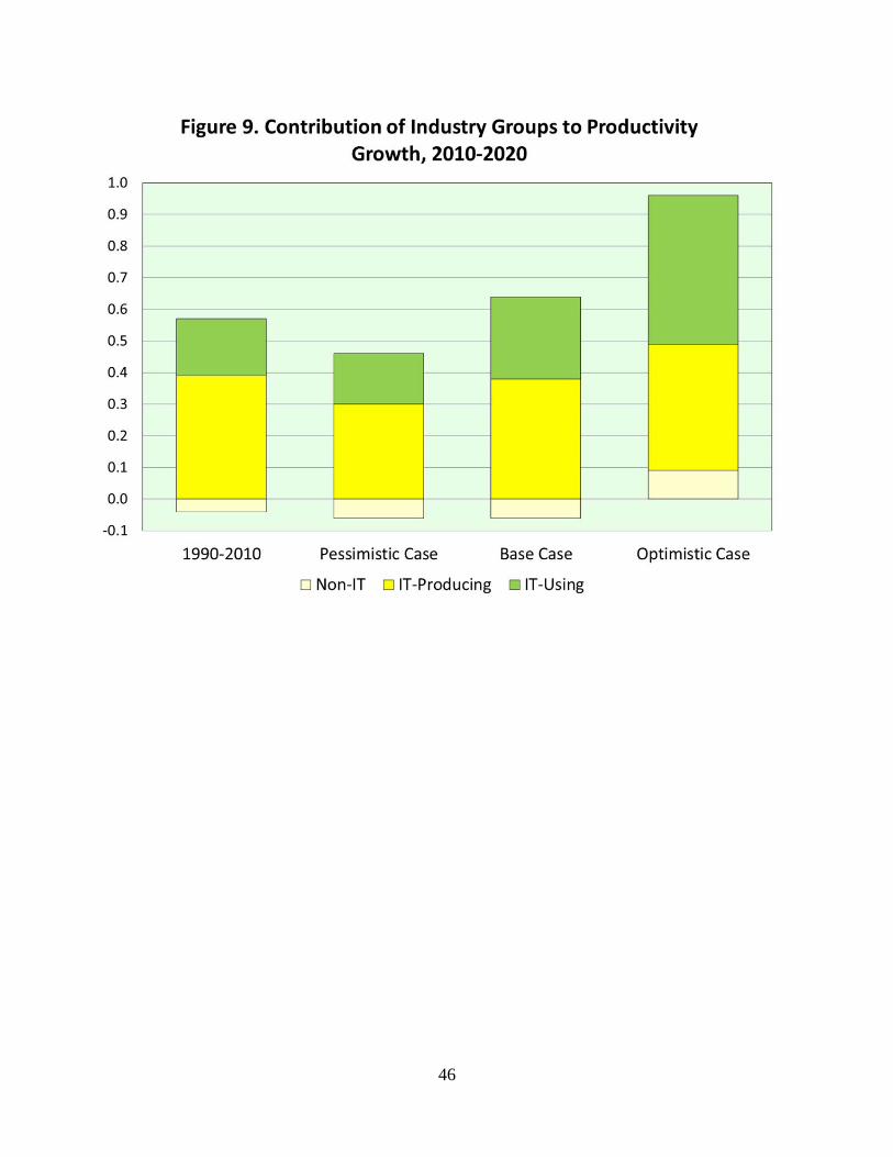
Our projections for the period 2010-2020 are summarized in Figures 9, 10 and 11. The

methodology is adapted from Jorgenson, Ho, and Stiroh (2008) to incorporate projections of total

factor productivity growth for IT-producing, IT-using, and Non-IT industries. Like Jorgenson, Ho,

and Stiroh, we present base case, pessimistic, and optimistic projections of future growth in

potential GDP. Our base case projections are based on the average contributions of total factor

productivity growth for the three sectors for the period 1995-2010. Our optimistic projections omit

the Great Recession period of 2005-2010, while our pessimistic projection includes the final five

years of the Long Slump, 1990-1995. We compare our projections with actual growth for 1990-

2010.

Our base case projection of growth in potential GDP in 2010-2020 is 1.93 percent per year,

compared with growth for 1990-2010 of 2.33 percent. The difference is due mainly to the projected

slowdown in the growth of labor quality. Actual labor quality growth is driven mainly by increases

in average educational attainment. Rising educational attainment has been a major driver of US

economic growth throughout the postwar period. However, educational attainment will reach a

plateau early in our projection period 2010-2020. Reduced labor quality growth will fall from 0.465

percent per year during 1990-2010 to only 0.077 percent per year in 2010-2020.

23

Our optimistic projection for potential US GDP growth is 2.63 percent per year during

2010-2020, compared with actual growth of 2.33 percent per year in 1990-2010. The contributions

of IT-using and Non-IT industries along with more rapid growth in capital quality are mainly

responsible for the increase in potential growth relative to actual growth. Our pessimistic projection

for potential growth is only 1.61 percent per year. The difference from our base case is due mainly

to a reduction in the projected growth of productivity in IT-producing and IT-using sectors and

slower improvement in capital quality.11

7. Conclusions

Our industry-level data set reveals that replication of established technologies through

growth of capital and labor inputs, recently through the growth of college-educated workers and

investments in both IT and Non-IT capital, explains by far the largest proportion of US economic

growth. International productivity comparisons reveal similar patterns for the world economy, its

major regions, and leading industrialized, developing, and emerging economies.12 Studies are now

underway to extend these comparisons to individual industries for the countries included in the

World KLEMS Initiative.13

Industry-level production accounts are now prepared on a regular basis by national

statistical agencies in Australia, Canada, Denmark, Finland, Italy, Mexico, The Netherlands, and

Sweden, as well as the United States. Augmented by production accounts from the EU (European

Union)-KLEMS (capital, labor, energy, materials, and services) study, described by Marcel

11 These projections are not directly comparable with those summarized by Byrne, Oliner and Sichel (2013), which are limited to nonfarm business. 12 See Jorgenson and Vu (2013). 13 See Jorgenson (2012), “The World KLEMS Initiative,” International Productivity Monitor, Fall, pp. 5-19.

24

Timmer, Robert Inklaar, Mary O’Mahony and Bart van Ark (2010), these accounts can be used in

international comparisons of sources of economic growth and patterns of structural change like

those presented by Jorgenson and Timmer (2011). The World-KLEMS Initiative will make it

possible to extend these comparisons to forty countries around the world, including important

developing and transition economies.

Conflicting interpretations of the Great Recession can be evaluated from the perspective of

our new data set. We do not share the technological pessimism of Cowen (2011) and Gordon

(2014), especially for the IT-producing industries. However, careful studies of developments of

semiconductor and computer technology show that the accelerated pace of innovation that began in

1995 reverted to the lower, but still substantial, rates of innovation in IT during the Long Slump

that ended in 1995.

Our findings also contribute to an understanding of the future potential for US economic

growth. Our new projections corroborate the perspective of Jorgenson, Ho, and Stiroh (2008), who

showed that the peak growth rates of the US Investment Boom of 1995-2000 were not sustainable.

However, our projections are less optimistic, due mainly to the slowing growth of the US labor

force and the virtual disappearance of improvements in labor quality. Negative productivity growth

during the Great Recession is transitory, but productivity growth is unlikely to return to the high

rates of the Investment Boom and the Jobless Recovery.

Finally, we conclude that the new findings presented in this paper have important

implications for US economic policy. Maintaining the gradual recovery from the Great Recession

will require a revival of investment in IT equipment and software and Non-IT capital as well.

Enhancing opportunities for employment is also essential, but this is likely to be most successful

25

for college-educated workers. These measures will contribute to closing the substantial remaining

gap between potential and actual output.

References

Aghion, Philippe, and Peter W. Howitt. 1998. Endogenous Growth Theory. Cambridge, MA: The

MIT Press.

Baily, Martin, James Manyika, and Shalabh Gupta. 2013. U.S. Productivity Growth: An

Optimistic Perspective. International Productivity Monitor25: 3-12.

Brynjolfsson, Erik, and Andrew McAfee.2014. The Second Machine Age: Work, Progress, and

Prosperity in a Time of Brilliant Technologies. New York: W. W. Norton.

Byrne, David, Steven Oliner, and Dan Sichel.2013.Is the Information Technology Revolution

Over? International Productivity Monitor 25: 20-36.

Cowen, Tyler. 2011.The Great Stagnation: How America Ate All the Low-Hanging Fruit, Got

Sick, and Will (Eventually) Feel Better.New York: Dutton.

Cowen, Tyler. 2013. Average is Over: Powering America Beyond the Age of the Great Stagnation,

New York: Dutton.

Domar, Evsey. 1961. On the Measurement of Technological Change. Economic Journal 71(284):

709-729.

Fernald, John. 2012. Productivity and Potential Output before, during, and after the Great

Recession. San Francisco: Federal Reserve Bank of San Francisco, September.

Fleck, Susan, Steven Rosenthal, Matthew Russell, Erich Strassner, and Lisa Usher. 2014. A

26

Prototype BEA/BLS Industry-Level Production Account for the United States.In Dale W.

Jorgenson, J. Steven Landefeld, and Paul Schreyer, eds., Measuring Economic Stability and

Progress. Chicago: University of Chicago Press: forthcoming.

Gordon, Robert. 2012. Is U.S. Economic Growth Over? Faltering Innovation and the Six

Headwinds. Cambridge, MA, National Bureau of Economic Research, Working Paper No

18315, August.

Gordon, Robert. 2014.The Demise of U.S. Economic Growth: Restatement, Rebuttal, and

Reflections. Cambridge, MA, National Bureau of Economic Research, Working Paper No

19895, February.

Harper, Michael, Brent Moulton, Steven Rosenthal, and David Wasshausen. 2009. Integrated

GDP-Productivity Accounts. American Economic Review 99(2): 74-79.

Hennessey, John L., and David A. Patterson. 2012. Computer Organization and Design, 4thed.

Waltham, MA: Morgan Kaufmann.

Jorgenson, Dale W. 1963. Capital Theory and Investment Behavior. American Economic Review

53(2): 247-259.

Jorgenson, Dale W. 1966. The Embodiment Hypothesis. Journal of Political Economy 74(1): 1-

17

Jorgenson, Dale W., ed., 2009. The Economics of Productivity. Northampton, MA: Edward Elgar.

Jorgenson, Dale W. 2012. The World KLEMS Initiative. International Productivity Monitor,

Fall: 5-19.

Jorgenson, Dale W., Frank M. Gollop, and Barbara M. Fraumeni. 1987. Productivity and U.S.

Economic Growth. Cambridge MA: Harvard University Press.

Jorgenson, Dale W., Mun S. Ho, and Jon Samuels. 2012. Information Technology and U.S.

27

Productivity Growth. In Matilde Mas and Robert Stehrer, eds., Industrial Productivity in

Europe, Northampton, MA, Edward Elgar: 34-65.

Jorgenson, Dale W., Mun S. Ho, and Kevin J. Stiroh. 2005. Information Technology and the

American Growth Resurgence. Cambridge, MA: The MIT Press.

Jorgenson, Dale W., Mun S. Ho, and Kevin J. Stiroh. 2008. A Retrospective Look at the U.S.

Productivity Growth Resurgence. Journal of Economic Perspectives 22(1): 3-24.

Jorgenson, Dale W., and Paul Schreyer. 2013. Industry-Level Productivity Measurement and the

2008 System of National Accounts. Review of Income and Wealth 58(4): 185-211.

Jorgenson, Dale W., and Marcel P. Timmer. 2011. Structural Change in Advanced Nations: A

New Set of Stylized Facts. Scandinavian Economic Journal 113(1): 1-29.

Jorgenson, Dale W., and Khuong M. Vu. 2013. The Emergence of the New Economic Order:

Economic Growth in the G7 and the G20. Journal of Policy Modeling, 35(2): 389-399.

Kuznets, Simon. 1971. Economic Growth of Nations: Total Output and Production Structure.

Cambridge, MA: Harvard University Press.

Manyika, James, David Hunt, Scott Nyquest, Jaana Remes, Vikrram Malhotra, Lenny Mendonca,

Byron August, and Samantha Test. 2011. Growth and Renewal in the United States, Washington, DC, McKinsey Global Institute, February.

Markoff, John. 2004. Intel’s Big Shift after Hitting Technical Wall. New York Times 153(52): 888.

Mas, Matilde, and Robert Stehrer, eds. 2012. Industrial Productivity in Europe.Northampton, MA,

Edward Elgar.

Mayerhauser, Nicole, and Erich Strassner. 2010.Preview of the Comprehensive Revision of the

Annual Industry Accounts. Survey of Current Business, 90(3): 21-34.

28

Pillai, Unni. 2013. A Model of Technological Progress in the Microprocessor Industry. Journal of

Industrial Economics 61(4): 877-912.

Schreyer, Paul. 2001. OECD Manual: Measuring Productivity: Measurement of Aggregate and

Industry-Level Productivity Growth. Paris: Organisation for Economic Development and

Cooperation.

Schreyer, Paul. 2009. OECD Manual: Measuring Capital. Paris: Organisation for Economic

Development and Cooperation.

Schumpeter, Joseph A. 1942. Capitalism, Socialism, and Democracy. New York: Harper.

Solow, Robert M. 1957. Technical Change and the Aggregate Production Function. Review of

Economics and Statistics 39(3):312-320.

Stiroh, Kevin J. 2002. Are ICT Spillovers Driving the New Economy? Review of Income and

Wealth 48(1): 33-57.

Syverson, Chad. 2011. What Determines Productivity? Journal of Economic Literature 49(2): 325-

365.

Syverson, Chad. 2013. Will History Repeat Itself? Comments on ‘Is the Information

Technology Revolution Over?’ International Productivity Monitor 25: 37-40.

Timmer, Marcel, Robert Inklaar, Mary O’Mahony, and Bart van Ark. 2010. Economic Growth in

Europe: A Comparative Industry Perspective, Cambridge, Cambridge University Press.

United Nations, Commission of the European Communities, International Monetary Fund,

Organisation for Economic Co-operation and Development, and World Bank. 2009.

System of National Accounts2008. New York, United Nations.

See: http://unstats.un.org/unsd/nationalaccount/sna2008.asp.

29

Table 1: Labor Characteristics by Industry, year 2010.

%college educated

price ($/hour)

% aged 16-35

% females

1 Farms 15.1 19.5 20.3 14.7

2 Forestry, fishing 16.4 16.6 30.8 15.3

3 Oil and gas extraction 38.6 79.5 14.6 22.2

4 Mining except oil and gas 11.8 39.2 20.2 8.8

5 Support activities for mining 26.0 37.6 25.8 13.8

6 Utilities 24.0 64.0 22.0 23.4

7 Construction 14.0 31.6 33.9 8.9

8 Wood products 12.2 26.0 32.9 15.1

9 Nonmetallic mineral products 18.1 32.3 26.0 19.7

10 Primary metals 17.7 39.7 26.0 13.5

11 Fabricated metal products 15.2 32.2 27.7 17.7

12 Machinery 24.5 38.7 25.6 19.4

13 Computer and electronic 62.3 56.7 31.0 30.3

14 Electrical equipment 44.2 52.5 26.4 30.9

15 Motor vehicles 23.6 37.9 28.4 21.8

16 Other transportation equip. 31.4 50.6 22.6 17.3

17 Furniture 15.6 26.3 31.5 24.3

18 Miscellaneous manufacturing 32.1 40.7 26.8 35.6

19 Food and tobacco 23.8 27.2 24.3 31.5

20 Textiles 14.0 25.6 26.5 45.2

21 Apparel and leather 17.6 27.0 27.4 55.9

22 Paper products 18.8 37.3 23.9 20.7

23 Printing 22.0 29.5 28.7 32.2

24 Petroleum and coal products 32.9 81.5 17.7 17.4

25 Chemical products 49.5 54.1 27.4 35.2

26 Plastics and rubber 16.4 30.7 30.2 28.5

27 Wholesale Trade 32.0 41.2 29.1 26.0

28 Retail Trade 15.8 23.0 35.4 42.0

29 Air transportation 38.2 49.5 28.6 35.9

30 Rail transportation 13.2 50.7 14.0 8.3

31 Water transportation 31.1 51.6 19.1 19.6

32 Truck transportation 8.6 28.0 24.6 11.1

33 Transit, ground psngr transportation 16.3 22.8 18.4 23.5

34 Pipeline transportation 32.8 65.6 17.5 18.4

35 Other transportation 19.7 33.5 34.1 20.7

36 Warehousing and storage 12.6 29.2 35.6 26.3

37 Publishing (incl. software) 60.2 52.5 38.1 42.8

38 Motion picture, sound recording 45.9 46.4 47.9 31.6

39 Broadcasting and telecom. 39.5 46.7 37.9 39.0

40 Information and data processing 55.4 55.0 47.7 40.8

41 Banks, credit intermediation 42.4 42.1 36.5 60.1

42 Securities, commodity contracts 71.9 120.6 38.3 35.2

43 Insurance carriers 46.6 48.7 28.5 56.4

44 Funds, trusts 71.0 99.4 40.7 37.3

45 Real estate 40.6 31.1 18.6 46.6

46 Rental and leasing 25.4 31.1 45.0 28.8

30

47 Legal services 65.5 57.5 29.0 53.1

48 Computer systems design 68.6 56.7 41.1 28.5

49 Professional and technical services 65.3 46.9 31.1 42.3

50 Management of companies 53.4 62.2 28.9 51.4

51 Administrative services 20.1 24.8 37.7 40.4

52 Waste management 10.2 32.5 33.9 14.3

53 Educational services 64.2 28.8 27.5 65.9

54 Ambulatory health care services 38.8 39.2 27.5 74.2

55 Hospitals and Nursing 30.4 28.4 28.1 79.5

56 Social assistance 30.0 18.8 36.1 86.7

57 Performing arts, spectator sports 48.7 53.8 29.1 43.8

58 Amusements and recreation 21.7 20.1 39.4 41.0

59 Accommodation 18.6 22.1 35.8 52.7

60 Food and drinking places 11.1 14.8 53.5 47.9

61 Other services except government 17.9 25.7 26.7 64.8

62 Federal General government 52.0 63.3 19.5 54.6

63 Federal Government enterprises 19.6 42.0 14.5 34.6

64 S&L Government enterprises 29.9 40.9 25.4 40.2

65 S&L General Government 48.6 36.3 23.5 61.2

31

32

33

34

35

36

37

38

39

40

41

42

43

44

45

46

47

48