Industry-Specific Productivity and Spatial Spillovers through

input-output linkages: evidence from Asia-Pacific Value Chain1

Weilin Liu

Institute of Economic and Social Development

Nankai University

Tianjin, China

liuwl@nankai.edu.cn

Robin C. Sickles

Department of Economics

Rice University

Houston, Texas USA

rsickles@rice.edu

Cambridge, MA 02138

October 17, 2019

1 We would like to thank Harry X. Wu for making available to us the China KLEMS data, Jaepil Han for providing the

code for the spatial-CSS estimations, and Will Grimme for his assistance in developing the graphical mapping software

and resulting figures that we have used to display the global value chains.

Abstract

This paper develops a theoretical growth model which combines spatial spillovers and

productivity growth heterogeneity at the industry-level. We exploit the global value chain

(GVC) linkages from inter-country input-output tables to describe the spatial

interdependencies in technology. The spillover effects from factor inputs and

Hicks-neutral technical change are separately identified in the model and decomposed

into domestic and international effects respectively. Country-specific production

functions are estimated using a spatial econometric specification for the industries of the

sample. Most of the spillover effects of factor inputs, which we measure in terms of

external factor elasticities, are found to be statistically and economically significant. The

spillover effects of technical change offered and received vary widely across industries

and contain information about the technological diffusion in GVC. Most prominently, the

spillover of productivity growth offered by US Electrical and Optical Equipment is

5.05%, which is the highest of all industries in our sample. Chinese Electrical and Optical

Equipment absorbs the spillover of productivity growth of 1.04% annually, with the

international component a relatively low 0.12%, which is substantially smaller than

Korea’s absorption of international spillovers that add 0.53% annually to this key

industry.

Keywords: Industry-specific productivity, spatial panel model, technological spillovers,

global value chain

JEL classification codes: C23, C51, C67, D24, O47, R15

1

1 Introduction

Over the past two decades the world economy has evolved rapidly and the network

structure of the global specialization has been dramatically transformed. The growth and

structure of individual national economies appear to depend critically on the growth rates

of other countries. Through the increasingly enhanced linkages of the production network,

a shock in one country can trigger misallocations of resources in other countries.

However, the way in which and the extent to which this complex and sophisticated

network of domestic and cross-border production-sharing activities impacts national

growth largely has been missing in the empirical economic growth literature.

Global value chains (GVCs) are the most important drivers of globalization (World

Bank et al., 2017). Currently nearly 70% of world trade in goods is composed of

intermediate inputs such as raw materials and capital components that are used to

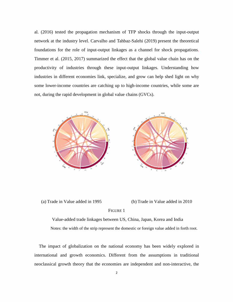
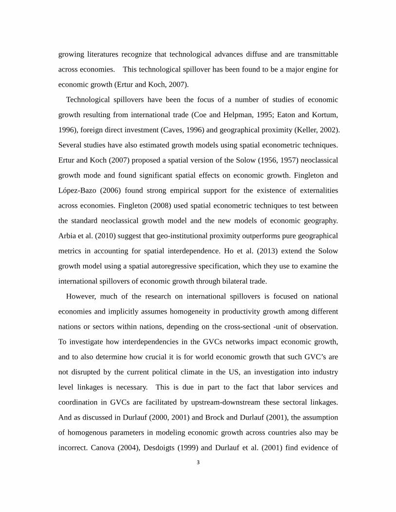
produce finished products.2. The linkages among major economies in the Asia-Pacific

area, which along with the US are the foci of our empirical analyses, measured by value

added exports based on the work of Johnson and Noguera (2012) are presented in

Figure13. The share of domestic linkages has declined for all the five countries from 1995

to 2010, the period we study, while foreign value added occupies an increasingly larger

share. The linkages between those countries and China from both the input and output

directions has expanded, implying significant changes in the pattern of the use of labor

services. Koopman et al. (2012, 2014) develop a detailed accounting framework to trace

the value-added flow based on a vertical specialization model and use the World

Input-Output tables to estimate domestic and foreign components in export. Acemoglu et

2 The UNSD Commodity Trade (UN Comtrade) database 3 Instead of the conventional measurement of trade by gross value of goods that may cause the “double-counting”

problem, we use Trade in Value added to construct the graph.

2

al. (2016) tested the propagation mechanism of TFP shocks through the input-output

network at the industry level. Carvalho and Tahbaz-Salehi (2019) present the theoretical

foundations for the role of input-output linkages as a channel for shock propagations.

Timmer et al. (2015, 2017) summarized the effect that the global value chain has on the

productivity of industries through these input-output linkages. Understanding how

industries in different economies link, specialize, and grow can help shed light on why

some lower-income countries are catching up to high-income countries, while some are

not, during the rapid development in global value chains (GVCs).

(a) Trade in Value added in 1995 (b) Trade in Value added in 2010

FIGURE 1

Value-added trade linkages between US, China, Japan, Korea and India

Notes: the width of the strip represent the domestic or foreign value added in forth root.

The impact of globalization on the national economy has been widely explored in

international and growth economics. Different from the assumptions in traditional

neoclassical growth theory that the economies are independent and non-interactive, the

3

growing literatures recognize that technological advances diffuse and are transmittable

across economies. This technological spillover has been found to be a major engine for

economic growth (Ertur and Koch, 2007).

Technological spillovers have been the focus of a number of studies of economic

growth resulting from international trade (Coe and Helpman, 1995; Eaton and Kortum,

1996), foreign direct investment (Caves, 1996) and geographical proximity (Keller, 2002).

Several studies have also estimated growth models using spatial econometric techniques.

Ertur and Koch (2007) proposed a spatial version of the Solow (1956, 1957) neoclassical

growth mode and found significant spatial effects on economic growth. Fingleton and

López-Bazo (2006) found strong empirical support for the existence of externalities

across economies. Fingleton (2008) used spatial econometric techniques to test between

the standard neoclassical growth model and the new models of economic geography.

Arbia et al. (2010) suggest that geo-institutional proximity outperforms pure geographical

metrics in accounting for spatial interdependence. Ho et al. (2013) extend the Solow

growth model using a spatial autoregressive specification, which they use to examine the

international spillovers of economic growth through bilateral trade.

However, much of the research on international spillovers is focused on national

economies and implicitly assumes homogeneity in productivity growth among different

nations or sectors within nations, depending on the cross-sectional -unit of observation.

To investigate how interdependencies in the GVCs networks impact economic growth,

and to also determine how crucial it is for world economic growth that such GVC’s are

not disrupted by the current political climate in the US, an investigation into industry

level linkages is necessary. This is due in part to the fact that labor services and

coordination in GVCs are facilitated by upstream-downstream these sectoral linkages.

And as discussed in Durlauf (2000, 2001) and Brock and Durlauf (2001), the assumption

of homogenous parameters in modeling economic growth across countries also may be

incorrect. Canova (2004), Desdoigts (1999) and Durlauf et al. (2001) find evidence of

4

parameter heterogeneity using different statistical methodologies. However, a

proliferation of free parameters in empirical modeling also may not allow one to explain

the structural factors and economic conditions behind the long-run growth phenomenon

(Durlauf and Quah, 1999, Ertur and Koch, 2007). Heterogeneity in productivity growth

among industries should be considered as such heterogeneity is intrinsic due to

techno-economical features of each distinct sector. Jorgenson et al. (2012) note the

influential power of some key industries and reveal the predominate role of IT-producing

and IT-using industries as sources of productivity growth. This industry perspective on

productivity and spillovers is particularly valuable as it provides intuitive information for

the policy design of selecting preferential industries and bridging the development gap

through encouraging the interaction in GVCs in order to promote technological advances.

A major contribution of this paper is to propose a new model for measuring the

industry-specific productivity and spillovers based on a spatial production function which

allows the productivity growth varies over the industries. We consider a neoclassical

output per worker growth model (Solow, 1956, 1957) as augmented, for example, by

Ertur and Koch (2007) to include spatial externalities in knowledge. Instead of using

geographical distance to construct the spatial weights matrix, we extract the input and

output flows based on the World Input-Output tables to measure economic distance

between industries within/across national economies. In so doing we are able to lift the

assumption of identical technical progress in all cross-sections by allowing for an

industry-specific function of time based on the estimation technique developed by

Cornwell et al. (1990) and Han and Sickles (2019).

We also provide more explicit insights on the spatial spillovers process in our empirical

analysis using a flexible spatial production function. The direct, indirect and total

marginal effects of the input factors and time trends are calculated to describe the role of

spillovers from input factors as well as how technical changes are distributed within the

GVCs network using both spatial autoregressive (SAR) and spatial Durbin (SDM)

5

production functions. We follow Glass et al. (2015) who estimate these effects based on

spatial translog production functions but calculate the industry-specific productivity

growth spillovers by distinguishing between knowledge receiving and offering, which

represent the two distinct directions of knowledge diffusion. Furthermore, in our global

value chain settings, we use local Ghosh matrices to identify the portion of indirect

effects that are transmitted within a country as well as the indirect effects that are

transferred across the borders respectively. Through our decomposition method, we are

able to distinguish between domestic and international spillovers.

This paper is organized as follows. In section 2 we set out the spatial production model

with heterogeneity in technical progress using SAR and SDM specifications, and then

explain our approach to measure the spatial spillovers of the inputs and Hicks-neutral

technical change. We also provide the methodology to decompose the domestic and

international spillovers using the local Ghosh matrices. Section 3 discusses our estimation

strategy. Section 4 presents the industry-level data of the countries we study and the

World Input-Output tables we used to construct the spatial weight matrix. In section 5 we

estimate the production function using our methodology and discuss the productivity

spillovers through Asia-Pacific value chain. Section 6 concludes.

2 Model

2.1 A production function with heterogeneity in technical progress

Consider an aggregate Cobb–Douglas production function with Hicks-neutral technical

change for industry i at time t exhibiting constant returns to scale in labor, capital and

intermediate input:

𝑌𝑌𝑖𝑖(𝑡𝑡) = 𝐴𝐴𝑖𝑖(𝑡𝑡)𝐾𝐾𝑖𝑖(𝑡𝑡)𝛼𝛼𝑀𝑀𝑖𝑖(𝑡𝑡)𝛽𝛽𝐿𝐿𝑖𝑖(𝑡𝑡)𝛾𝛾, 𝑖𝑖 = 1,⋯ ,𝑁𝑁, 𝑡𝑡 = 1,⋯ ,𝑇𝑇, (1)

6

where 𝑌𝑌𝑖𝑖(𝑡𝑡) is the total output, 𝐾𝐾𝑖𝑖(𝑡𝑡), 𝑀𝑀𝑖𝑖(𝑡𝑡) and 𝐿𝐿𝑖𝑖(𝑡𝑡) are the capital, labor and

intermediate input respectively and 𝛼𝛼 + 𝛽𝛽 + 𝛾𝛾 = 1. 𝐴𝐴𝑖𝑖(𝑡𝑡) is the aggregate level of

technology, which differs among industries and time periods.

The technology 𝐴𝐴𝑖𝑖(𝑡𝑡) can be described in the following form:

𝐴𝐴𝑖𝑖(𝑡𝑡) = Ω𝑖𝑖(t) = Ω(0)𝑖𝑖𝑒𝑒𝑅𝑅(𝑡𝑡)′𝛿𝛿𝑖𝑖 (2)

where 𝑅𝑅(𝑡𝑡) is an L×1 time-varying component that globally affects all industries, and

𝛿𝛿𝑖𝑖 is an L×1 the coefficients that depend on i. Ω𝑖𝑖(0) is the individual initial technology

state. We extend the Solow model (Solow, 1956; Swan, 1956; Ertur and Koch, 2007) of

identical technical progress in all industries by allowing for an industry-specific time

trend. We can then write the non-spatial production function per worker as:

𝑦𝑦𝑖𝑖(𝑡𝑡) = 𝐴𝐴𝑖𝑖(𝑡𝑡)𝑘𝑘𝑖𝑖(𝑡𝑡)𝛼𝛼𝑚𝑚𝑖𝑖(𝑡𝑡)𝛽𝛽 = Ω𝑖𝑖(0)𝑒𝑒𝑅𝑅(𝑡𝑡)′𝛿𝛿𝑖𝑖𝑘𝑘𝑖𝑖(𝑡𝑡)𝛼𝛼𝑚𝑚𝑖𝑖(𝑡𝑡)𝛽𝛽 (3)

where 𝑦𝑦𝑖𝑖(𝑡𝑡) = 𝑌𝑌𝑖𝑖(𝑡𝑡)/𝐿𝐿𝑖𝑖(𝑡𝑡), 𝑘𝑘𝑖𝑖(𝑡𝑡) = 𝐾𝐾𝑖𝑖(𝑡𝑡)/𝐿𝐿𝑖𝑖(𝑡𝑡), 𝑚𝑚𝑖𝑖(𝑡𝑡) = 𝑀𝑀𝑖𝑖(𝑡𝑡)/𝐿𝐿𝑖𝑖(𝑡𝑡).

Decomposing 𝑅𝑅(𝑡𝑡)′𝛿𝛿𝑖𝑖 into a global time trend 𝑅𝑅(𝑡𝑡)′𝛿𝛿𝑔𝑔 and an industry-specific term

𝑅𝑅(𝑡𝑡)′𝑢𝑢𝑖𝑖 and then taking the logarithm of Eq. (3), we have the following linear regression

model in the form of Cornwell et al. (1990)4:

ln𝑦𝑦𝑖𝑖𝑡𝑡 = ln𝑘𝑘𝑖𝑖𝑡𝑡𝛼𝛼 + ln𝑚𝑚𝑖𝑖𝑡𝑡𝛽𝛽 + lnΩ𝑖𝑖(0) + 𝑅𝑅𝑡𝑡′𝛿𝛿𝑔𝑔 + 𝑅𝑅𝑡𝑡′𝑢𝑢𝑖𝑖 + 𝑣𝑣𝑖𝑖𝑡𝑡 (4)

where 𝑢𝑢𝑖𝑖 are assumed to be iid zero mean random variables with covariance matrix Δ,

and 𝑣𝑣𝑖𝑖𝑡𝑡 is the usual disturbance term assumed to a random noise following iid N(0, σ𝑣𝑣2).

This model assumes the heterogeneous initial state and progress of technology. However,

we note that if there are no heterogeneities, i.e., Ω𝑖𝑖(0) and 𝑢𝑢𝑖𝑖 are constant, then the

production function can be written in the usual form and the Eq. (4) reduces to the

standard panel data model with a time trend.

4 In a series of papers Park, Sickles, and Simar (1998, 2003, 2007) showed, among other things, that the time varying

CSS and time invariant Schmidt and Sickles (1984) panel data estimators for the stochastic panel frontier were

semiparametric efficient for the slope coefficients in the class of linear panel data models with correlated random

effects. See also Sickles and Zelenuyk (2019) for a more extensive discussion of these and many other estimators for

average and frontier production models.

7

2.2 Spatial model with technology spillover

To account for the technology spillover through the linkage of industries, the effect of

cross-sectional dependence should be considered in the production functions. Ertur and

Koch (2009) modeled the technology as a function of a common global time trend, per

worker capital and a spatial lag of a country’s neighbor’s technology. Here we relax the

assumption of Hicks-neutral technical change by allowing each industry i to have

industry-specific technical progress Ω𝑖𝑖(t) while at the same time allowing the industry

to absorb knowledge diffusion from its neighbors. We assume that knowledge diffusion is

influenced by the strength of linkage 𝑤𝑤𝑖𝑖𝑖𝑖 with neighbor-industry j and neighbor-industry

j’s labor productivity 𝑦𝑦𝑖𝑖(𝑡𝑡). The Solow residual then can be written as

𝐴𝐴𝑖𝑖(t) = Ω𝑖𝑖(t)∏ 𝑦𝑦𝑖𝑖(𝑡𝑡)𝜌𝜌𝜌𝜌𝑖𝑖𝑖𝑖𝑁𝑁𝑖𝑖≠𝑖𝑖 = Ω𝑖𝑖(0)𝑒𝑒𝑅𝑅(𝑡𝑡)′𝛿𝛿𝑖𝑖 ∏ 𝑦𝑦𝑖𝑖(𝑡𝑡)𝜌𝜌𝜌𝜌𝑖𝑖𝑖𝑖𝑁𝑁

𝑖𝑖≠𝑖𝑖 ,

(5)

And this leads to the following production function per worker:

𝑦𝑦𝑖𝑖(𝑡𝑡) = Ω𝑖𝑖(0)𝑒𝑒𝑅𝑅(𝑡𝑡)′𝛿𝛿𝑖𝑖 ∏ 𝑦𝑦𝑖𝑖(𝑡𝑡)𝜌𝜌𝜌𝜌𝑖𝑖𝑖𝑖𝑁𝑁𝑖𝑖≠𝑖𝑖 𝑘𝑘𝑖𝑖(𝑡𝑡)𝛼𝛼𝑚𝑚𝑖𝑖(𝑡𝑡)𝛽𝛽. (6)

Taking the logarithms of the expression, we obtain a Spatial Autoregressive form

regression model as follows:

ln𝑦𝑦𝑖𝑖𝑡𝑡 = 𝜌𝜌∑ 𝑤𝑤𝑖𝑖𝑖𝑖ln𝑦𝑦𝑖𝑖𝑡𝑡𝑁𝑁𝑖𝑖=1 + ln𝑘𝑘𝑖𝑖𝑡𝑡𝛼𝛼 + ln𝑚𝑚𝑖𝑖𝑡𝑡𝛽𝛽 + lnΩ𝑖𝑖0 + 𝑅𝑅𝑡𝑡′𝛿𝛿𝑔𝑔 + 𝑅𝑅𝑡𝑡′𝑢𝑢𝑖𝑖 + 𝑣𝑣𝑖𝑖𝑡𝑡, (7)

which we rewrite in matrix form as

𝑦𝑦 = 𝜌𝜌(𝑊𝑊𝑁𝑁⨂𝐼𝐼𝑇𝑇)𝑦𝑦 + 𝑘𝑘𝛼𝛼 + 𝑚𝑚𝛽𝛽 + ω0 + 𝑟𝑟𝛿𝛿𝑔𝑔 + 𝑞𝑞𝑞𝑞 + 𝑉𝑉, (8)

where 𝑦𝑦 , 𝑘𝑘 , 𝑚𝑚 and 𝑉𝑉 are 𝑁𝑁𝑇𝑇 × 1 vectors, ω0 = Ω𝑖𝑖0⨂𝜄𝜄𝑇𝑇 , 𝜄𝜄𝑇𝑇 is 𝑇𝑇 dimensional

vector of ones, 𝑟𝑟 = 𝜄𝜄𝑁𝑁⨂𝑅𝑅 , 𝜄𝜄𝑁𝑁 is 𝑁𝑁 dimensional vector of ones,

𝑅𝑅 = (𝑅𝑅1,𝑅𝑅2,⋯ ,𝑅𝑅𝑇𝑇)′, 𝑞𝑞 = 𝜄𝜄𝑁𝑁⨂𝑑𝑑𝑖𝑖𝑑𝑑𝑑𝑑(𝑅𝑅), is 𝑁𝑁𝑇𝑇 × 𝐿𝐿𝑁𝑁 matrix, 𝛿𝛿𝑔𝑔 is 𝐿𝐿 × 1 vector, and

𝑞𝑞 is a 𝐿𝐿𝑁𝑁 × 1 vector.

In a more general case, we can assume technical spillovers are not just influenced by

the neighbor’s labor productivity, but by the neighbor’s technology 𝐴𝐴𝑖𝑖(𝑡𝑡), input levels of

8

per-worker physical capital 𝑘𝑘𝑖𝑖(𝑡𝑡), and per-worker intermediate input 𝑚𝑚𝑖𝑖(𝑡𝑡). We also can

consider the spatial linkages that may have effects on an industry’s output when its

neighbor changes its input. This leads to the following expression for technology:

𝐴𝐴𝑖𝑖(t) = Ω𝑖𝑖(t)∏ 𝐴𝐴𝑖𝑖(𝑡𝑡)𝜌𝜌𝜌𝜌𝑖𝑖𝑖𝑖𝑁𝑁𝑖𝑖≠𝑖𝑖 ∏ 𝑘𝑘𝑖𝑖(𝑡𝑡)𝜙𝜙𝜌𝜌𝑖𝑖𝑖𝑖𝑁𝑁

𝑖𝑖≠𝑖𝑖 ∏ 𝑚𝑚𝑖𝑖(𝑡𝑡)𝜑𝜑𝜌𝜌𝑖𝑖𝑖𝑖𝑁𝑁𝑖𝑖≠𝑖𝑖

= Ω𝑖𝑖(t)∏ 𝑦𝑦𝑖𝑖(𝑡𝑡)/𝑘𝑘𝑖𝑖(𝑡𝑡)𝛼𝛼𝑚𝑚𝑖𝑖(𝑡𝑡)𝛽𝛽𝜌𝜌𝜌𝜌𝑖𝑖𝑖𝑖𝑁𝑁

𝑖𝑖≠𝑖𝑖 ∏ 𝑘𝑘𝑖𝑖(𝑡𝑡)𝜙𝜙𝜌𝜌𝑖𝑖𝑖𝑖𝑁𝑁𝑖𝑖≠𝑖𝑖 ∏ 𝑚𝑚𝑖𝑖(𝑡𝑡)𝜑𝜑𝜌𝜌𝑖𝑖𝑖𝑖𝑁𝑁

𝑖𝑖≠𝑖𝑖

= Ω𝑖𝑖(0)𝑒𝑒𝑅𝑅(𝑡𝑡)′𝛿𝛿𝑖𝑖 ∏ 𝑦𝑦𝑖𝑖(𝑡𝑡)𝜌𝜌𝜌𝜌𝑖𝑖𝑖𝑖𝑁𝑁𝑖𝑖≠𝑖𝑖 ∏ 𝑘𝑘𝑖𝑖(𝑡𝑡)(𝜙𝜙−𝛼𝛼𝜌𝜌)𝜌𝜌𝑖𝑖𝑖𝑖𝑁𝑁

𝑖𝑖≠𝑖𝑖 ∏ 𝑚𝑚𝑖𝑖(𝑡𝑡)(𝜑𝜑−𝛽𝛽𝜌𝜌)𝜌𝜌𝑖𝑖𝑖𝑖𝑁𝑁𝑖𝑖≠𝑖𝑖 . (9)

Replacing this expression in the production function, then take logarithms, we obtain

the production function in a Spatial Durbin form5:

ln𝑦𝑦𝑖𝑖𝑡𝑡 = 𝜌𝜌∑ 𝑤𝑤𝑖𝑖𝑖𝑖ln𝑦𝑦𝑖𝑖𝑡𝑡𝑁𝑁𝑖𝑖=1 + ln𝑘𝑘𝑖𝑖𝑡𝑡𝛼𝛼 + ln𝑚𝑚𝑖𝑖𝑡𝑡𝛽𝛽 + lnΩ𝑖𝑖0 + 𝑅𝑅𝑡𝑡′𝛿𝛿𝑔𝑔 + 𝑅𝑅𝑡𝑡′𝑢𝑢𝑖𝑖 + 𝑣𝑣𝑖𝑖𝑡𝑡

+∑ 𝑤𝑤𝑖𝑖𝑖𝑖ln𝑘𝑘𝑖𝑖𝑡𝑡𝑁𝑁𝑖𝑖=1 (𝜙𝜙 − 𝜌𝜌𝛼𝛼) + ∑ 𝑤𝑤𝑖𝑖𝑖𝑖ln𝑚𝑚𝑖𝑖𝑡𝑡

𝑁𝑁𝑖𝑖=1 (𝜑𝜑 − 𝜌𝜌𝛽𝛽). (10)

Likewise, the matrix form of (10) is given by

𝑦𝑦 = 𝜌𝜌(𝑊𝑊𝑁𝑁⨂𝐼𝐼𝑇𝑇)𝑦𝑦 + 𝑘𝑘𝛼𝛼 + 𝑚𝑚𝛽𝛽 + ω0 + 𝑟𝑟𝛿𝛿𝑔𝑔 + 𝑞𝑞𝑞𝑞 + 𝑉𝑉

+(𝜙𝜙 − 𝜌𝜌𝛼𝛼)(𝑊𝑊𝑁𝑁⨂𝐼𝐼𝑇𝑇)𝑘𝑘 + (𝜑𝜑 − 𝜌𝜌𝛽𝛽)(𝑊𝑊𝑁𝑁⨂𝐼𝐼𝑇𝑇)𝑚𝑚. (11)

2.3 Technology Spillovers and Spatial Elasticities

As demonstrated in LeSage and Pace (2009), for spatial models the usual interpretation of

𝛼𝛼 and 𝛽𝛽 as elasticities of input factors is not valid. They instead suggest the following

approach to calculate direct, indirect, and total marginal effects. First resolve the linear

system for 𝑦𝑦, if 𝜌𝜌 ≠ 0 and if 1/𝜌𝜌 is not an eigenvalue of 𝑊𝑊𝑁𝑁⨂𝐼𝐼𝑇𝑇, and rewrite Eq. (8)

and (11) as (12) and (13):

𝑦𝑦 = 𝛼𝛼(𝛪𝛪 − 𝜌𝜌𝑊𝑊𝑁𝑁⨂𝐼𝐼𝑇𝑇)−1𝑘𝑘 + 𝛽𝛽(𝛪𝛪 − 𝜌𝜌𝑊𝑊𝑁𝑁⨂𝐼𝐼𝑇𝑇)−1𝑚𝑚

+(𝛪𝛪 − 𝜌𝜌𝑊𝑊𝑁𝑁⨂𝐼𝐼𝑇𝑇)−1 ω0 + 𝑟𝑟𝛿𝛿𝑔𝑔 + 𝑞𝑞𝑞𝑞 + 𝑉𝑉 (12)

𝑦𝑦 = (𝛪𝛪 − 𝜌𝜌𝑊𝑊𝑁𝑁⨂𝐼𝐼𝑇𝑇)−1[𝛼𝛼𝐼𝐼 + (𝜙𝜙 − 𝜌𝜌𝛼𝛼)𝑊𝑊𝑁𝑁⨂𝐼𝐼𝑇𝑇]𝑘𝑘 + (𝛪𝛪 − 𝜌𝜌𝑊𝑊𝑁𝑁⨂𝐼𝐼𝑇𝑇)−1 5 Strictly Eq.(12) is a partial spatial Durbin model, the local spatial function of Hicks-neutral technological change is

omitted since the introduction of ∑ 𝑤𝑤𝑖𝑖𝑖𝑖𝑅𝑅𝑡𝑡′𝛿𝛿𝑔𝑔𝑁𝑁𝑖𝑖=1 would be perfect collinearity with 𝑅𝑅𝑡𝑡′𝛿𝛿𝑔𝑔.

9

[𝛽𝛽𝐼𝐼 + (𝜑𝜑 − 𝜌𝜌𝛽𝛽)𝑊𝑊𝑁𝑁⨂𝐼𝐼𝑇𝑇]𝑚𝑚 + (𝛪𝛪 − 𝜌𝜌𝑊𝑊𝑁𝑁⨂𝐼𝐼𝑇𝑇)−1 ω0 + 𝑟𝑟𝛿𝛿𝑔𝑔 + 𝑞𝑞𝑞𝑞 + 𝑉𝑉. (13)

Differentiating Eq. (13) with respect to per-worker capital yields the following matrix

of direct and indirect effects for each industry, where the right-hand side of Eq. (14b) is

independent of the time index:

𝐸𝐸𝑘𝑘 ≡ 𝜕𝜕ln𝑦𝑦𝜕𝜕ln𝑘𝑘1

, 𝜕𝜕ln𝑦𝑦𝜕𝜕ln𝑘𝑘2

,⋯ , 𝜕𝜕ln𝑦𝑦𝜕𝜕ln𝑘𝑘𝑁𝑁

𝑡𝑡

=

⎣⎢⎢⎢⎢⎡

𝜕𝜕ln𝑦𝑦1𝜕𝜕ln𝑘𝑘1

𝜕𝜕ln𝑦𝑦1𝜕𝜕ln𝑘𝑘2

⋯ 𝜕𝜕ln𝑦𝑦1𝜕𝜕ln𝑘𝑘𝑁𝑁

𝜕𝜕ln𝑦𝑦2𝜕𝜕ln𝑘𝑘1

𝜕𝜕ln𝑦𝑦2𝜕𝜕ln𝑘𝑘2

⋯ 𝜕𝜕ln𝑦𝑦2𝜕𝜕ln𝑘𝑘𝑁𝑁

⋮ ⋮ ⋱ ⋮ 𝜕𝜕ln𝑦𝑦𝑁𝑁𝜕𝜕ln𝑘𝑘1

𝜕𝜕ln𝑦𝑦𝑁𝑁𝜕𝜕ln𝑘𝑘2

⋯ 𝜕𝜕ln𝑦𝑦𝑁𝑁𝜕𝜕ln𝑘𝑘𝑁𝑁 ⎦

⎥⎥⎥⎥⎤

𝑡𝑡

(14a)

= (𝛪𝛪𝑁𝑁 − 𝜌𝜌𝑊𝑊𝑁𝑁)−1

𝛼𝛼 𝑤𝑤12(𝜙𝜙 − 𝜌𝜌𝛼𝛼) … 𝑤𝑤21(𝜙𝜙 − 𝜌𝜌𝛼𝛼) 𝛼𝛼 …

⋮ ⋮ ⋱

𝑤𝑤1𝑁𝑁(𝜙𝜙 − 𝜌𝜌𝛼𝛼)𝑤𝑤2𝑁𝑁(𝜙𝜙 − 𝜌𝜌𝛼𝛼)

⋮𝑤𝑤𝑁𝑁1(𝜙𝜙 − 𝜌𝜌𝛼𝛼) 𝑤𝑤𝑁𝑁2(𝜙𝜙 − 𝜌𝜌𝛼𝛼) ⋯ 𝛼𝛼

. (14b)

Then the mean direct effect of per-worker capital for all the industries, which we

denote 𝑒𝑒𝑘𝑘𝐷𝐷𝑖𝑖𝐷𝐷, is the average of the diagonal elements of the matrix in Eq. (14b) for the

SDM model. The indirect effects of per-worker capital, which we denote 𝑒𝑒𝑘𝑘𝐼𝐼𝐼𝐼𝐼𝐼, are the

average row-sum of the off-diagonal elements of the matrix in Eq. (14b). The mean total

effects of per-worker capital is 𝑒𝑒𝑘𝑘𝑇𝑇𝑇𝑇𝑡𝑡 = 𝑒𝑒𝑘𝑘𝐷𝐷𝑖𝑖𝐷𝐷 + 𝑒𝑒𝑘𝑘𝐼𝐼𝐼𝐼𝐼𝐼 (LeSage and Pace, 2009). In the SAR

model, the direct, indirect and total effects can also be calculated using Eq. (14b) but with

the off-diagonal elements set equal to zero. Likewise, we can calculate the effects for

per-worker intermediate 𝑒𝑒𝑚𝑚𝐷𝐷𝑖𝑖𝐷𝐷 , 𝑒𝑒𝑚𝑚𝐼𝐼𝐼𝐼𝐼𝐼 and 𝑒𝑒𝑚𝑚𝑇𝑇𝑇𝑇𝑡𝑡 . Under the assumption of constant

returns to scale, the effect for 𝑘𝑘 and 𝑚𝑚 are equivalent to the elasticities of capital and

intermediate inputs. However, in the spatial model the direct elasticity also includes

feedback effects when the input changes in industry 𝑖𝑖 affect a neighbor industry’s output,

and this effect on neighbor industries rebounds and affects industry 𝑖𝑖’s output via the

inter-industry linkage. The indirect elasticity refers to the percentage change in

industry 𝑖𝑖’s output due to a percentage increase in the sum of the input across all the other

𝑁𝑁 − 1 industries. Finally, the calculation of total elasticity is based on all 𝑁𝑁 industries

10

in the sample simultaneously changing their input, not just industry 𝑖𝑖 or the other 𝑁𝑁 − 1

units (Glass, et al., 2015). It can be shown that the direct elasticity of labor is 𝑒𝑒𝑙𝑙𝐷𝐷𝑖𝑖𝐷𝐷 =

1 − 𝑒𝑒𝑘𝑘𝐷𝐷𝑖𝑖𝐷𝐷 − 𝑒𝑒𝑚𝑚𝐷𝐷𝑖𝑖𝐷𝐷 and the indirect elasticity of labor is 𝑒𝑒𝑙𝑙𝐼𝐼𝐼𝐼𝐼𝐼 = −𝑒𝑒𝑘𝑘𝐼𝐼𝐼𝐼𝐼𝐼 − 𝑒𝑒𝑚𝑚𝐼𝐼𝐼𝐼𝐼𝐼. Therefore

the total elasticity of labor 𝑒𝑒𝑙𝑙𝑇𝑇𝑇𝑇𝑡𝑡 = 1 − 𝑒𝑒𝑘𝑘𝑇𝑇𝑇𝑇𝑡𝑡 − 𝑒𝑒𝑚𝑚𝑇𝑇𝑇𝑇𝑡𝑡 and constant returns to scale still

holds in the spatial settings6.

In the same way, we can describe the Hicks-neutral technical change over time and the

magnitude of spillovers between the industries through spatial correlation. By

differentiating Eq. (13) with respect to the time trend, this productivity change spillover

can be measured by the indirect marginal effect from the spatial model:

𝑑𝑑𝑡𝑡 ≡ 𝜕𝜕ln𝑦𝑦𝜕𝜕𝑡𝑡𝑡𝑡

= (𝛪𝛪𝑁𝑁 − 𝜌𝜌𝑊𝑊𝑁𝑁)−1

⎣⎢⎢⎢⎢⎡

𝜕𝜕𝑅𝑅𝑡𝑡′

𝜕𝜕𝑡𝑡𝛿𝛿1 0 ⋯ 0

0 𝜕𝜕𝑅𝑅𝑡𝑡′

𝜕𝜕𝑡𝑡𝛿𝛿2 ⋯ 0

⋮ ⋮ ⋱ ⋮ 0 0 ⋯ 𝜕𝜕𝑅𝑅𝑡𝑡

′

𝜕𝜕𝑡𝑡𝛿𝛿𝐼𝐼⎦⎥⎥⎥⎥⎤

𝑡𝑡

(15a)

=

⎣⎢⎢⎢⎢⎡ 𝑤𝑤11

𝜕𝜕𝑅𝑅𝑡𝑡′

𝜕𝜕𝑡𝑡𝛿𝛿1 𝑤𝑤12

𝜕𝜕𝑅𝑅𝑡𝑡′

𝜕𝜕𝑡𝑡𝛿𝛿2 ⋯ 𝑤𝑤1𝐼𝐼 𝜕𝜕𝑅𝑅𝑡𝑡

′

𝜕𝜕𝑡𝑡𝛿𝛿𝐼𝐼

𝑤𝑤21𝜕𝜕𝑅𝑅𝑡𝑡′

𝜕𝜕𝑡𝑡𝛿𝛿1 𝑤𝑤22

𝜕𝜕𝑅𝑅𝑡𝑡′

𝜕𝜕𝑡𝑡𝛿𝛿2 ⋯ 𝑤𝑤2𝐼𝐼 𝜕𝜕𝑅𝑅𝑡𝑡

′

𝜕𝜕𝑡𝑡𝛿𝛿𝐼𝐼

⋮ ⋮ ⋱ ⋮ 𝑤𝑤𝐼𝐼1

𝜕𝜕𝑅𝑅𝑡𝑡′

𝜕𝜕𝑡𝑡𝛿𝛿1 𝑤𝑤𝐼𝐼2

𝜕𝜕𝑅𝑅𝑡𝑡′

𝜕𝜕𝑡𝑡𝛿𝛿2 ⋯ 𝑤𝑤𝐼𝐼𝐼𝐼 𝜕𝜕𝑅𝑅𝑡𝑡

′

𝜕𝜕𝑡𝑡𝛿𝛿𝐼𝐼⎦⎥⎥⎥⎥⎤

𝑡𝑡

, (15b)

where 𝑤𝑤𝑖𝑖𝑖𝑖 is the element of (𝛪𝛪𝑁𝑁 − 𝜌𝜌𝑊𝑊𝑁𝑁)−1. The diagonal elements of the matrix in Eq.

(15b), which we denote as 𝑑𝑑𝐷𝐷𝑖𝑖𝑟𝑟𝑡𝑡, is the direct effect, which represents the productivity

change for industry 𝑖𝑖 itself at time 𝑡𝑡. However, the indirect effect has two different

interpretations depending on which directions to sum the off-diagonal elements. The

row-sum of off-diagonal elements, which we denote 𝑑𝑑𝐼𝐼𝑔𝑔𝑑𝑑𝑡𝑡𝐷𝐷, represents the aggregate

spillover that each industry received from all of its neighbors through the spatial linkages

while the compound productivity change for industry 𝑖𝑖, measured by the summation of

the direct effect and indirect effect received from all other industries, is denoted as

6 Please see Appendix A for the derivations of the elasticities.

11

𝑑𝑑𝑇𝑇𝑔𝑔𝑡𝑡𝑡𝑡𝐷𝐷 = 𝑑𝑑𝐷𝐷𝑖𝑖𝑟𝑟𝑡𝑡 + 𝑑𝑑𝐼𝐼𝑔𝑔𝑑𝑑𝑡𝑡𝐷𝐷. The column-sum of off-diagonal elements, which we denote

𝑑𝑑𝐼𝐼𝑔𝑔𝑑𝑑𝑡𝑡𝑇𝑇 , represents the aggregate spillover that each industry provides its neighbors.

Likewise, the compound productivity change for industry 𝑖𝑖 measured by the summation

of direct effect and indirect effect provided to all other industries is denoted as

𝑑𝑑𝑇𝑇𝑔𝑔𝑡𝑡𝑡𝑡𝑇𝑇 = 𝑑𝑑𝐷𝐷𝑖𝑖𝑟𝑟𝑡𝑡 + 𝑑𝑑𝐼𝐼𝑔𝑔𝑑𝑑𝑡𝑡𝑇𝑇.

2.4 Decomposition of technology spillovers by domestic and international effect

In the production system of the global value chain, knowledge spillovers not only involve

industries within a country, but knowledge spillovers also cross national borders. Suppose

there are two countries 𝑠𝑠 and 𝑟𝑟 , with 𝑄𝑄𝑠𝑠 and 𝑄𝑄𝐷𝐷 industries respectively, in a

production system with a global value chain, then the spatial weight matrix 𝑊𝑊𝑁𝑁 can be

split into a block structure such as:

𝑊𝑊𝑁𝑁 ≡ 𝑊𝑊𝑠𝑠𝑠𝑠 𝑊𝑊𝑠𝑠𝐷𝐷𝑊𝑊𝐷𝐷𝑠𝑠 𝑊𝑊𝐷𝐷𝐷𝐷

, (16)

where 𝑊𝑊𝑠𝑠𝑠𝑠 is 𝑄𝑄𝑠𝑠 × 𝑄𝑄𝑠𝑠 matrix, 𝑊𝑊𝑠𝑠𝐷𝐷 is 𝑄𝑄𝑠𝑠 × 𝑄𝑄𝐷𝐷 matrix, 𝑊𝑊𝐷𝐷𝑠𝑠 is 𝑄𝑄𝐷𝐷 × 𝑄𝑄𝑠𝑠 matrix and

𝑊𝑊𝐷𝐷𝐷𝐷 is 𝑄𝑄𝐷𝐷 × 𝑄𝑄𝐷𝐷 matrix. 𝑊𝑊𝑠𝑠𝑠𝑠 and 𝑊𝑊𝐷𝐷𝐷𝐷 represent the linkages of the industries within

the border of each country, and 𝑊𝑊𝑠𝑠𝐷𝐷 and 𝑊𝑊𝐷𝐷𝑠𝑠 represent the linkages of industries across

country borders.

In order to decompose the different spillover effects into portion involving the

domestic value chain and a portion involving the international value chain, we define the

left multiplier in Eq.(14b) as the global multiplier 𝐺𝐺 ≡ (𝛪𝛪𝑁𝑁 − 𝜌𝜌𝑊𝑊𝑁𝑁)−1, which represents

the global interactions that include the feedbacks through higher order of linkages though

neighbors, and define the local multiplier of country 𝑠𝑠 as 𝐻𝐻𝑠𝑠𝑠𝑠 ≡ 𝛪𝛪𝑄𝑄 − 𝜌𝜌𝑊𝑊𝑠𝑠𝑠𝑠−1

. This

latter term we call the local multiplier of a country and it represents the domestic

interactions of industries within the border of country 𝑠𝑠. We can define the local

12

multiplier of country 𝑟𝑟 as 𝐻𝐻𝐷𝐷𝐷𝐷 in the same way. Then the global multiplier 𝐺𝐺 can be

decomposed into7:

𝐺𝐺 ≡ 𝐺𝐺𝑠𝑠𝑠𝑠 𝐺𝐺𝑠𝑠𝐷𝐷𝐺𝐺𝐷𝐷𝑠𝑠 𝐺𝐺𝐷𝐷𝐷𝐷

= 𝐻𝐻𝑠𝑠𝑠𝑠 00 𝐻𝐻𝐷𝐷𝐷𝐷

+ 𝜌𝜌𝑊𝑊𝑠𝑠𝐷𝐷𝐺𝐺𝐷𝐷𝑠𝑠𝐻𝐻𝑠𝑠𝑠𝑠 𝐺𝐺𝑠𝑠𝐷𝐷𝐺𝐺𝐷𝐷𝑠𝑠 𝜌𝜌𝑊𝑊𝐷𝐷𝑠𝑠𝐺𝐺𝑠𝑠𝐷𝐷𝐻𝐻𝐷𝐷𝐷𝐷

, (17)

where the first matrix composed by 𝐻𝐻𝑠𝑠𝑠𝑠 and 𝐻𝐻𝐷𝐷𝐷𝐷 in the diagonal in the right of Eq.(17)

corresponds to the domestic multiplier, and the second matrix corresponds to the

international multiplier which captures the international spillover processes: the

off-diagonal blocks represent the diffusions between the two countries and the diagonal

blocks represent the country’s diffusion firstly go aboard and then feedback to itself.

That is, the sub-matrix of 𝜌𝜌𝑊𝑊𝑠𝑠𝐷𝐷𝐺𝐺𝐷𝐷𝑠𝑠𝐻𝐻𝑠𝑠𝑠𝑠 corresponds to the process of the technology

firstly transmitted from country 𝑠𝑠 to country 𝑟𝑟 directly and then retransmitted back to

country 𝑠𝑠 and diffused among the industries within country 𝑠𝑠.

Following Eq.(14b), the matrix 𝐸𝐸𝑘𝑘 measuring the direct and indirect effects of

per-worker capital can be decomposed into a domestic effect, 𝐸𝐸𝐷𝐷𝑘𝑘, and an international

effect, 𝐸𝐸𝐼𝐼𝑘𝑘.

𝐸𝐸𝐷𝐷𝑘𝑘 ≡ 𝐻𝐻𝑠𝑠𝑠𝑠 00 𝐻𝐻𝐷𝐷𝐷𝐷

𝛼𝛼 𝑤𝑤12(𝜙𝜙 − 𝜌𝜌𝛼𝛼) … 𝑤𝑤21(𝜙𝜙 − 𝜌𝜌𝛼𝛼) 𝛼𝛼 …

⋮ ⋮ ⋱

𝑤𝑤1𝑁𝑁(𝜙𝜙 − 𝜌𝜌𝛼𝛼)𝑤𝑤2𝑁𝑁(𝜙𝜙 − 𝜌𝜌𝛼𝛼)

⋮𝑤𝑤𝑁𝑁1(𝜙𝜙 − 𝜌𝜌𝛼𝛼) 𝑤𝑤𝑁𝑁2(𝜙𝜙 − 𝜌𝜌𝛼𝛼) ⋯ 𝛼𝛼

(18)

𝐸𝐸𝐼𝐼𝑘𝑘 ≡

𝜌𝜌𝑊𝑊𝑠𝑠𝐷𝐷𝐺𝐺𝐷𝐷𝑠𝑠𝐻𝐻𝑠𝑠𝑠𝑠 𝐺𝐺𝑠𝑠𝐷𝐷𝐺𝐺𝐷𝐷𝑠𝑠 𝜌𝜌𝑊𝑊𝐷𝐷𝑠𝑠𝐺𝐺𝑠𝑠𝐷𝐷𝐻𝐻𝐷𝐷𝐷𝐷

𝛼𝛼 𝑤𝑤12(𝜙𝜙 − 𝜌𝜌𝛼𝛼) … 𝑤𝑤21(𝜙𝜙 − 𝜌𝜌𝛼𝛼) 𝛼𝛼 …

⋮ ⋮ ⋱

𝑤𝑤1𝑁𝑁(𝜙𝜙 − 𝜌𝜌𝛼𝛼)𝑤𝑤2𝑁𝑁(𝜙𝜙 − 𝜌𝜌𝛼𝛼)

⋮𝑤𝑤𝑁𝑁1(𝜙𝜙 − 𝜌𝜌𝛼𝛼) 𝑤𝑤𝑁𝑁2(𝜙𝜙 − 𝜌𝜌𝛼𝛼) ⋯ 𝛼𝛼

. (19)

With the matrices of 𝐸𝐸𝐷𝐷𝑘𝑘 and 𝐸𝐸𝐼𝐼𝑘𝑘, we can calculate the mean direct, indirect and

total domestic effects of per-worker capital expressed as 𝑒𝑒𝑑𝑑𝑘𝑘𝐷𝐷𝑖𝑖𝐷𝐷 , 𝑒𝑒𝑑𝑑𝑘𝑘𝐼𝐼𝐼𝐼𝐼𝐼 and 𝑒𝑒𝑑𝑑𝑘𝑘𝑇𝑇𝑇𝑇𝑡𝑡

7 With the definition of 𝐺𝐺, we have: (𝛪𝛪𝑁𝑁 − 𝜌𝜌𝑊𝑊𝑁𝑁) 𝐺𝐺 = 𝛪𝛪𝑄𝑄 − 𝜌𝜌𝑊𝑊𝑠𝑠𝑠𝑠 𝑊𝑊𝑠𝑠𝐷𝐷

𝑊𝑊𝐷𝐷𝑠𝑠 𝛪𝛪𝑄𝑄 − 𝜌𝜌𝑊𝑊𝐷𝐷𝐷𝐷 𝐺𝐺𝑠𝑠𝑠𝑠 𝐺𝐺𝑠𝑠𝐷𝐷𝐺𝐺𝐷𝐷𝑠𝑠 𝐺𝐺𝐷𝐷𝐷𝐷

= 𝛪𝛪𝑄𝑄 00 𝛪𝛪𝑄𝑄

then we can

get the relationship of 𝐺𝐺𝑠𝑠𝑠𝑠 and 𝐻𝐻𝑠𝑠𝑠𝑠 as 𝛪𝛪𝑄𝑄 + 𝜌𝜌𝑊𝑊𝑠𝑠𝐷𝐷𝐺𝐺𝐷𝐷𝑠𝑠𝐻𝐻𝑠𝑠𝑠𝑠 = 𝐺𝐺𝑠𝑠𝑠𝑠 and the relationship of 𝐺𝐺𝐷𝐷𝐷𝐷 and 𝐻𝐻𝐷𝐷𝐷𝐷 𝛪𝛪𝑄𝑄 +

𝜌𝜌𝑊𝑊𝐷𝐷𝑠𝑠𝐺𝐺𝑠𝑠𝐷𝐷𝐻𝐻𝐷𝐷𝐷𝐷 = 𝐺𝐺𝐷𝐷𝐷𝐷.

13

respectively, and direct, indirect and total international effects of per-worker capital

expressed as 𝑒𝑒𝑖𝑖𝑘𝑘𝐷𝐷𝑖𝑖𝐷𝐷 , 𝑒𝑒𝑖𝑖𝑘𝑘𝐼𝐼𝐼𝐼𝐼𝐼 and 𝑒𝑒𝑖𝑖𝑘𝑘𝑇𝑇𝑇𝑇𝑡𝑡 respectively. Correspondingly, we can get the

decomposition results for other inputs and the time trend of productivity.

This two-country setting easily can be extended to a multi-country scenario by setting

𝐸𝐸𝐷𝐷𝑘𝑘 as a block diagonal matrix composed of any given number of country blocks.

With 𝐸𝐸𝐼𝐼𝑘𝑘 = 𝐸𝐸𝑘𝑘 − 𝐸𝐸𝐷𝐷𝑘𝑘, one can calculate the corresponding effects for the capital input.

3 Estimation

We outline the estimator for the SAR specification developed in the previous section.

The SAR specification associated with Eq.(7) is:

01

,N

it ij jt it i t t i itj

y w y X Z R R u vρ β γ δ=

′ ′ ′ ′= + + + + +∑ (20)

where wij is the ijth element of the (N×N) spatial weights matrix WN, to be given

exogenously, ui is assumed to be an iid zero mean random variable with covariance

matrix∆ , and itν is an iid disturbance term that follows a 2(0, )N νσ distribution. The

matrix form of Eq. (20) is given by8:

0( ) ,N Ty W I y X QU Vρ β γ δ= ⊗ + + + + +Z R (21)

where y and V are 1NT × vectors, X is an NT K× matrix,

( )TZ ι= ⊗Z , Z is an N J× matrix, Tι is a T dimensional vector of

ones, ( )N Rι= ⊗R , 1 2( , , , )TR R R R ′= , ( )NQ diag Rι= ⊗ is an NT LN×

8The observations are stacked with t being the fast-running index and i the slow-running index, i.e.,

11 12 1 1( , , , , , , , )T N NTy y y y y y ′= . The order of observations is very important for writing correct codes.

In typical spatial analysis literature, the slower index is over time, the faster index is over individuals.

14

matrix, β is a 1K × vector, γ is a 1J × vector, 0δ is an 1L×

vector, and U is an 1LN × vector.

The Spatial Durbin specification associated with Eq. (10) is:

01 1

,N N

it ij jt it ij jt i t t i itj j

y w y X w X Z R R u vρ β λ γ δ= =

′ ′ ′ ′ ′= + + + + + +∑ ∑ (22)

where ijw is the ij th element of ( )N N× spatial weights matrix NW , to be

given exogenously, iu is assumed as iid zero mean random variables with

covariance matrix ∆ , and itv , is a random noise following 2(0, )vN σ 9. In

addition, the matrix form of Eq.(22) is given by:

0( ) ( ) ,N T N Ty W I y X W I X QU Vρ β γ δ= ⊗ + + ⊗ + + + +Z Rλ (23)

where y and V are 1NT × vectors, X is an NT K× matrix,

( )TZ ι= ⊗Z , Z is N J× matrix, Tι is a T dimensional vector of ones,

( )N Rι= ⊗R , 1 2( , , , )TR R R R ′= , ( )NQ diag Rι= ⊗ is an NT LN× matrix,

β is a 1K × vector, γ is a 1J × vector, 0δ is an 1L× vector, and

U is an 1LN × vector.

Production functions are typically estimated by using various parametric,

nonparametric, and semi-parametric techniques. A standard approach to production

function estimation is to adhere to the average production technology instead of the

best-practice technology, which is accomplished in the stochastic frontier literature by

neglecting the assumption that all producers are cost or profit efficient. Minimal

differences, if any differences exist at all, usually appear in the estimates of the basic

production model parameters, such as in output elasticities, among others. However, the 9We may want to specify different spatial correlation structures on dependent variable and independent variables.

However, we use the same dependence structure for both variables.

15

stochastic frontier analysis (SFA) approach can decompose the Solow-type residual into

two components. The identification of the decomposition of TFP growth into separate

efficiency and technical change components is based on the assumption that the average

production function represents the maximum level of output given the levels of inputs on

the average. Shifts in this average level of productivity over time, which are usually

represented as a common trend by using either a time variable or a time index, indicates

technical change. Inefficiency is interpreted as the productivity of a unit at a specific time

period relative to the average best-practice production frontier, and it typically includes a

one-sided term (negative) that represents the short-fall in a firm's average production

relative to a benchmark set by the most efficient firm. One-sided distributions, such as

half-normal, truncated normal, exponential, or gamma distribution, are often used in

parametric models. Schmidt and Sickles (SS) (1984) and Cornwell, Schmidt, and Sickles

(CSS) (1990) suggested the avoidance of strong distributional assumptions by utilizing

the structure of a panel production frontier. Schmidt and Sickles (1984) assumed

inefficiency to be time-invariant and unit-specific, while Cornwell et al. (1990) relaxed

the time-invariant assumption by introducing a flexibly parametrized function of time,

thereby replacing individual fixed effects. In the present study, we follow the CSS

method as it allows us to estimate time-varying efficiency without requiring further

distributional assumptions on the one-sided efficiency term.

The non-spatial CSS model, given in Eq. (4) can be estimated via three techniques:

within transformation, generalized least squares, and efficient instrumental variable

approach. However, the extended models (Eqs.7 and 10) have several difficulties in

estimation because they include additional spatially correlated variables. A

quasi-maximum likelihood estimation (QMLE) is thus used in our analysis. QMLE can

provide robust standard errors against misspecification of the error distributions. QMLE

enables us to minimize the number of parameters to be estimated via the concentrated

likelihood function instead of using the full likelihood function. We typically substitute

16

the closed-form solutions of a set of parameters into the likelihood function, and the

resultant concentrated likelihood function becomes a function of spatial coefficient

parameters only. The optimization with the concentrated likelihood is known to give the

same maximum likelihood estimates after maximizing the full likelihood. We will

outline the estimation procedure here briefly. The details are presented in Appendix B

and are from Han (2016).

We can find closed-form solutions for the parameters, except for the spatial

autoregressive parameter ρ , by using the first-order conditions of the likelihood

functions of Eqs.7 and 10. The spatial parameters of λ are the coefficients of the

spatially weighted independent variables. We treat the spatially weighted independent

variables as additional regressors. The substitution of the closed-form solutions into the

likelihood functions gives the concentrated likelihood functions with ρ as the only

unknown variable. However, ρ can be obtained by maximizing the concentrated

likelihood function. Hence, all other parameters can be found by using ρ . Once we

obtain the estimates of the parameters , , iβ ρ δ , and 2vσ , we can recursively solve

for an estimate of itα , although we cannot separately identify 0δ and iu . By

using the estimate of itα , we can obtain the relative inefficiency measure following SS

and CSS. In particular, from Eq.??, we know the estimate of itα is ˆˆ .it t iRα δ′=

Estimates of the frontier intercept tα and the time-dependent relative inefficiency

measure itu can be derived as10:

10Hence, the relative efficiency score can be written as ˆitu

itEFF e−= .

17

ˆ ˆmax( ),

ˆ ˆˆ .

t jtj

it t itu

α α

α α

=

= −

4 Data

International comparisons of the patterns of output, input and productivity are very

challenging (Jorgenson, et al., 2012). We integrate several databases for the empirical

analysis of the productivities under the global value chain labor-division network. The

countries in our sample are United States, China, Japan, Korea and India, which are the

main economies in the Asia & Pacific area. The international production network has

rapidly developed among these countries since 1980’s. We extract the output measures of

gross output and input measures of capital service, labor service and intermediate input

from the KLEMS database.

The WORLD KLEMS database provided the quantity and price indices data for the

United States, Japan, Korea and India. 2005 is the reference year11. Data for China

are collected from the China Industrial Productivity (CIP) Database, which provided the

real and nominal gross output and intermediate input by reconstructing China’s

input-output table (Wu and Keiko, 2015; Wu, 2015; Wu, et al, 2015). We calculate the

growth rates for gross output and intermediate input in constant prices by single deflation.

CIP also provided the capital and labor input indices which are consistent with the

KLEMS database and we converted the reference year from 1990 to 2005.

The inter-country input-output data are draw from the World Input-Output database

(WIOD) database. We match and aggregate some industries since there are some

difference in the industry classification across the databases of KLEMS, WIOD and CIP,

although they are all broadly consistent with the ISIC revision 3. The nominal volumes

11 In Asia KLEMS database, the reference years of the indices for Korea is 2000, and the labor and capital indices for

Korea is 1981. The reference years for other indices are 2005, which is in accordance with US KLEMS data.

18

for each index are used to generate the weights for calculating the input and output

indices of the aggregated industries. We omitted non-market economy industries, which

are mostly local public services that include Housing, Public Administration and Defense,

Education, Health and Social Work, Other Community, Social and Personal Services12.

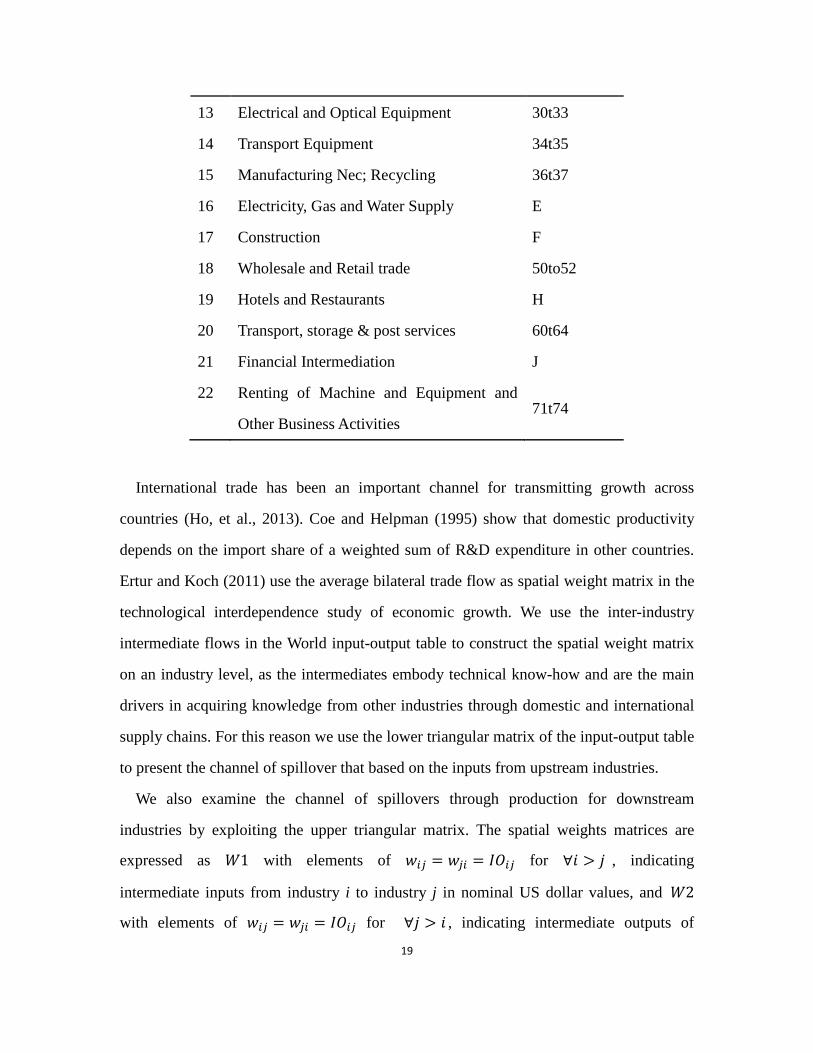
The industry classifications we use are listed in Table 1. The sample period is 1980-2010.

We extract industry-level linkages among the five countries from the input-output table

for 1995, which is the mid-year of the sample period.

Table 1: Industry classifications and codes

No. Industry ISIC Rev. 3

1 Agriculture, Hunting, Forestry and Fishing AtB

2 Mining and Quarrying C

3 Food , Beverages and Tobacco 15t16

4 Textiles and Textile, Leather, leather and

footwear

17t19

5 Wood and of Wood and Cork 20

6 Pulp, Paper, Paper , Printing and

Publishing

21t22

7 Coke, Refined Petroleum and Nuclear Fuel 23

8 Chemicals and Chemical 24

9 Rubber and Plastics 25

10 Other Non-Metallic Mineral 26

11 Basic Metals and Fabricated Metal 27t28

12 Machinery, Nec 29

12 We also remove the whole and retail trade, Renting of Machine and Equipment and Other Business Activities in

India for the data are missing.

19

13 Electrical and Optical Equipment 30t33

14 Transport Equipment 34t35

15 Manufacturing Nec; Recycling 36t37

16 Electricity, Gas and Water Supply E

17 Construction F

18 Wholesale and Retail trade 50to52

19 Hotels and Restaurants H

20 Transport, storage & post services 60t64

21 Financial Intermediation J

22 Renting of Machine and Equipment and

Other Business Activities 71t74

International trade has been an important channel for transmitting growth across

countries (Ho, et al., 2013). Coe and Helpman (1995) show that domestic productivity

depends on the import share of a weighted sum of R&D expenditure in other countries.

Ertur and Koch (2011) use the average bilateral trade flow as spatial weight matrix in the

technological interdependence study of economic growth. We use the inter-industry

intermediate flows in the World input-output table to construct the spatial weight matrix

on an industry level, as the intermediates embody technical know-how and are the main

drivers in acquiring knowledge from other industries through domestic and international

supply chains. For this reason we use the lower triangular matrix of the input-output table

to present the channel of spillover that based on the inputs from upstream industries.

We also examine the channel of spillovers through production for downstream

industries by exploiting the upper triangular matrix. The spatial weights matrices are

expressed as 𝑊𝑊1 with elements of 𝑤𝑤𝑖𝑖𝑖𝑖 = 𝑤𝑤𝑖𝑖𝑖𝑖 = 𝐼𝐼𝐼𝐼𝑖𝑖𝑖𝑖 for ∀𝑖𝑖 > 𝑗𝑗 , indicating

intermediate inputs from industry i to industry j in nominal US dollar values, and 𝑊𝑊2

with elements of 𝑤𝑤𝑖𝑖𝑖𝑖 = 𝑤𝑤𝑖𝑖𝑖𝑖 = 𝐼𝐼𝐼𝐼𝑖𝑖𝑖𝑖 for ∀𝑗𝑗 > 𝑖𝑖 , indicating intermediate outputs of

20

industry i to industry j. The diagonal elements of 𝑊𝑊1 and 𝑊𝑊2 are all 0. Elhorst (2001)

propose a normalization method by dividing the matrix by the maximum eigenvalue

when row normalization may cause the matrix to lose its economic interpretation of

distance decay. However, in this paper, we assumes that the productivity spillover is

dependent on the share weighted sum of the productivity of their intermediate suppliers

(or users)13, which is consistent with the seminal article of Coe and Helpman (1995).

Therefore, 𝑊𝑊1 and 𝑊𝑊2 are row normalized to generate the spatial weight matrix.

5 Empirical results

We model the industry-specific productivity growth with 𝑅𝑅(𝑡𝑡)′𝛿𝛿𝑖𝑖 = 𝛿𝛿𝑖𝑖𝑡𝑡 to and country

dummies to control for different technology states in different countries. To avoid

possible endogeneity problems between input factor levels and productivity, we lag the

inputs one period (Ackerberg, et al., 2015). In order to control for possible endogeneity

between spatial linkages and output, we use the input-output table in the mid-year of the

sample period (i.e. 1995) to construct the spatial weight matrices following the spatial

literature that address the constructions of socioeconomic weight matrices (Case, et al.,

1993; Cohen and Paul, 2004).

13 This is more intuitive than assuming spillover to be proportional to the value of linkage, by normalizing

the weight matrix by maximum eigenvalue, i.e. small enterprise may be more influenced by its major

supplier or customer than big enterprise, although big company may use more products from the same

supplier (or sell more products to the same customer) than the small company.

21

5.1 Estimations of Production Functions

In Table 1, we provide estimates of the Solow-type production function for the

industries for our selected countries, without a spatial specification in Eq. (4). We use

the Cornwell, Schmidt, Sickles (CSS) (1990) estimator. The CSS estimator with

time-varying fixed effects (CSSW), and its special case of time-invariant fixed effects

introduced by Schmidt and Sickles (SS), are based on standard projections used in the

average production approach but with the added option to decompose the error term from

the within residuals after, e.g., a fixed effects regression. In the stochastic frontier

analysis paradigm, when no scale economies exist, and they do not appear to be in this

analysis, TFP change = technical change (coefficient of year dummies) + technical

efficiency change (CSS estimated efficiency). When estimating the average production

function, we estimate the coefficients and TFP as the Solow residual. One other aspect of

the SS and the CSS slope estimates is that they also are semiparametric efficient when the

joint distribution of the effects and the regressors are specified non-parametrically and are

equivalent to the standard panel fixed effect estimates when the fixed effects and means

of the regressors are correlated, such as in the Mundlak and Pesaran setups (Park, Sickles,

and Simar (JOE, 1998, 2003, 2007). However, use of the decomposition of TFP into

efficiency and an innovation component is often useful and informative.

The dependent variable is gross-output index. All coefficient estimates for the factor

inputs are statistically significant. The coefficients of inputs can be interpreted as output

elasticities. The elasticity of intermediate input is the largest, while capital is the smallest.

We also can estimate the parameters for the time trend of productivity in the CSS random

effects model (CSSG). Hausman-Wu statistic for the fixed effects v. random effects

specification of the CSS estimator is 22.408 with a p-value of 0.803 and thus we do not

reject the time-varying random effects specification. The coefficient on the Time

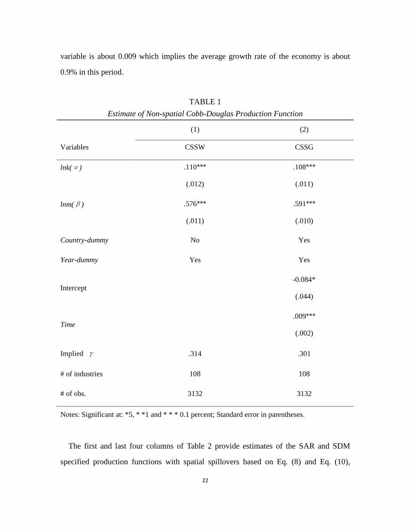
22

variable is about 0.009 which implies the average growth rate of the economy is about

0.9% in this period.

TABLE 1 Estimate of Non-spatial Cobb-Douglas Production Function

(1) (2)

Variables CSSW CSSG

lnk(α) .110***

(.012)

.108***

(.011)

lnm(β) .576***

(.011)

.591***

(.010)

Country-dummy No Yes

Year-dummy Yes Yes

Intercept -0.084*

(.044)

Time .009***

(.002)

Implied γ .314 .301

# of industries 108 108

# of obs. 3132 3132

Notes: Significant at: *5, * *1 and * * * 0.1 percent; Standard error in parentheses.

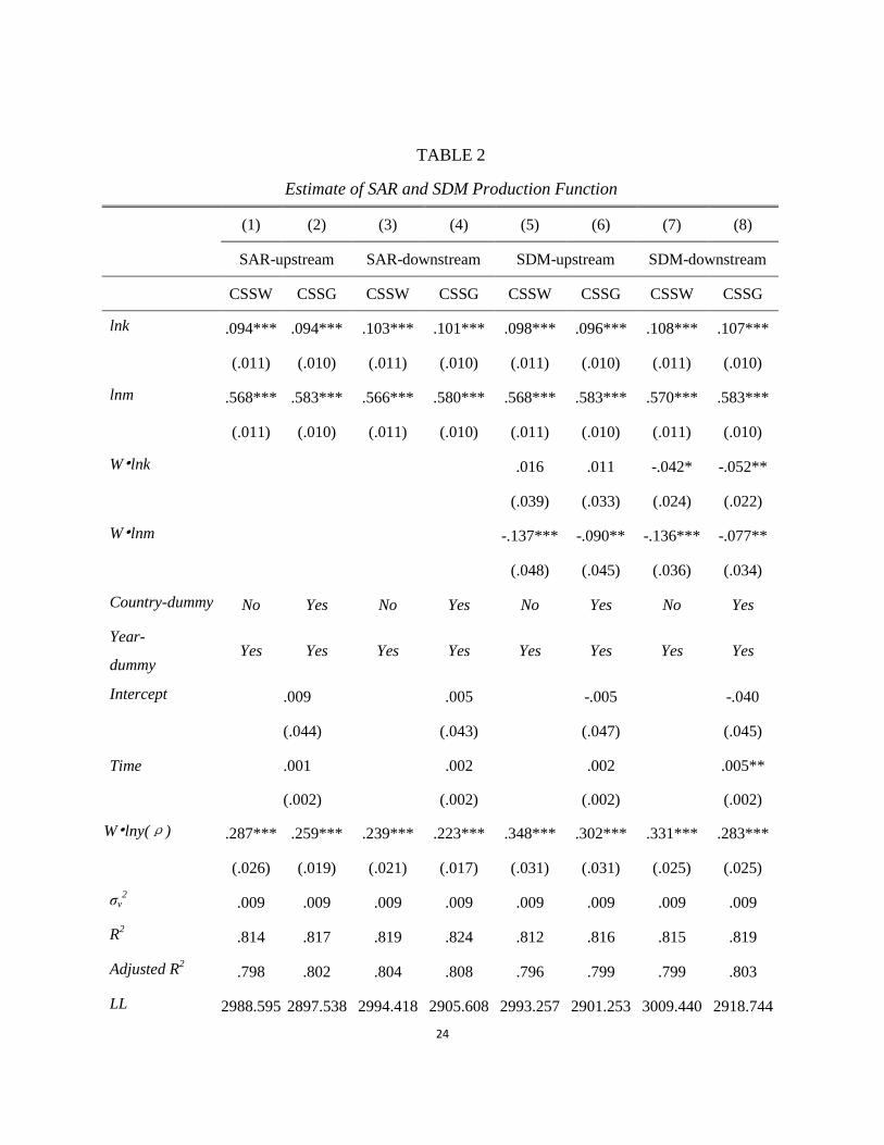
The first and last four columns of Table 2 provide estimates of the SAR and SDM

specified production functions with spatial spillovers based on Eq. (8) and Eq. (10),

23

respectively. All of the coefficients for the factor inputs in the SAR and SDM

specifications are statistically significant at the 1% significance level. The coefficient of

the spatially lagged dependent variableρ is estimated in a range of 0.223 to 0.287 for

SAR and 0.283 to 0.348 for SDM.. The parameters of ϕ and φ, which represent the local

spatial relationships of factor inputs, can be calculated based on the expressions in Eq.

(10). In the SDM-upstream model, ϕ and φ are both positive, whereas the coefficient of

the spatially weighted capital input is not significant. In the SDM-downstream model, the

coefficients of the spatially weighted independent variables are significant, and ϕ and φ

are negative and positive respectively, which suggests that the neighbour’s capital and

intermediate inputs have a negative and positive effect respectively for the productivity of

an industry. The intuitive implication for a negative effect is related to the indirect effect

that we more fully explain in Section 5.2 below.

24

TABLE 2

Estimate of SAR and SDM Production Function

(1) (2) (3) (4) (5) (6) (7) (8)

SAR-upstream SAR-downstream SDM-upstream SDM-downstream

CSSW CSSG CSSW CSSG CSSW CSSG CSSW CSSG

lnk .094*** .094*** .103*** .101*** .098*** .096*** .108*** .107***

(.011) (.010) (.011) (.010) (.011) (.010) (.011) (.010)

lnm .568*** .583*** .566*** .580*** .568*** .583*** .570*** .583***

(.011) (.010) (.011) (.010) (.011) (.010) (.011) (.010)

W•lnk .016 .011 -.042* -.052**

(.039) (.033) (.024) (.022)

W•lnm -.137*** -.090** -.136*** -.077**

(.048) (.045) (.036) (.034)

Country-dummy No Yes No Yes No Yes No Yes

Year-

dummy Yes Yes Yes Yes Yes Yes Yes Yes

Intercept .009 .005 -.005 -.040

(.044) (.043) (.047) (.045)

Time .001 .002 .002 .005**

(.002) (.002) (.002) (.002)

W•lny(ρ) .287*** .259*** .239*** .223*** .348*** .302*** .331*** .283***

(.026) (.019) (.021) (.017) (.031) (.031) (.025) (.025)

σv2 .009 .009 .009 .009 .009 .009 .009 .009

R2 .814 .817 .819 .824 .812 .816 .815 .819

Adjusted R2 .798 .802 .804 .808 .796 .799 .799 .803

LL 2988.595 2897.538 2994.418 2905.608 2993.257 2901.253 3009.440 2918.744

25

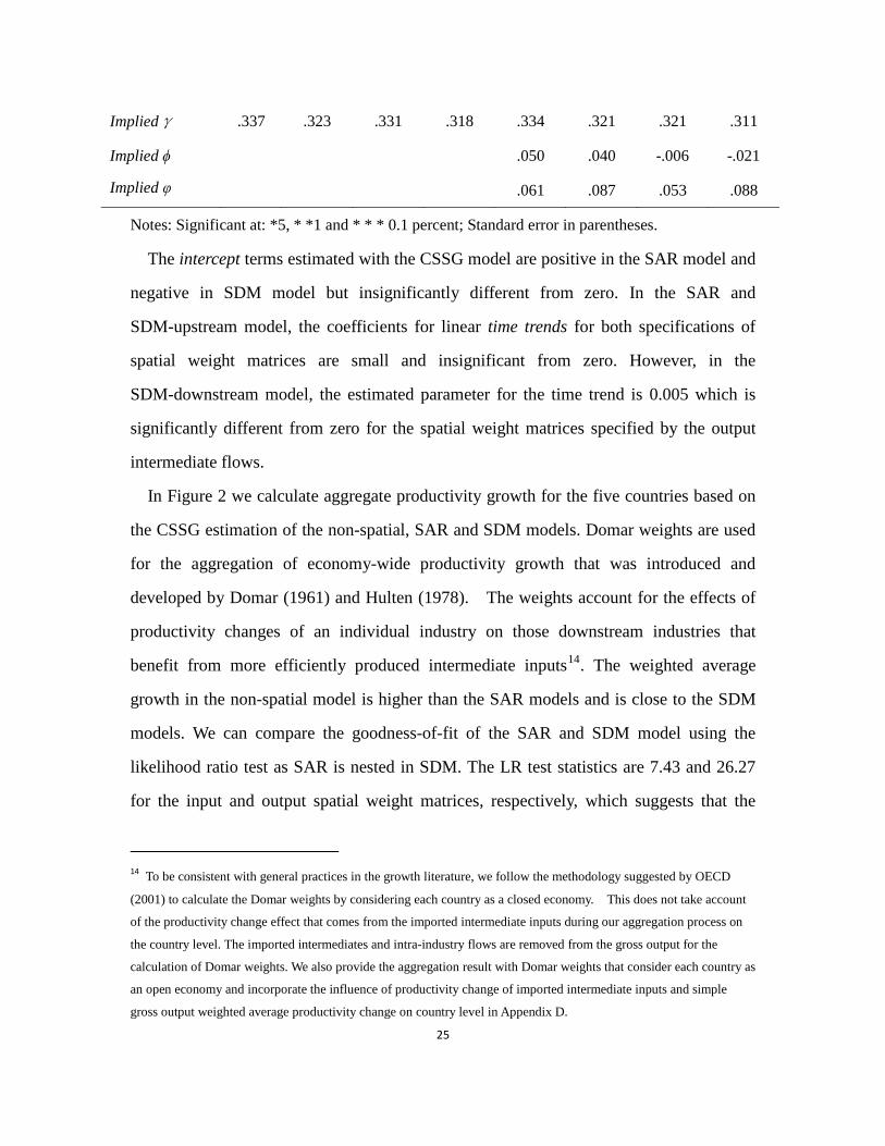
Impliedγ .337 .323 .331 .318 .334 .321 .321 .311

Implied ϕ .050 .040 -.006 -.021

Implied φ .061 .087 .053 .088

Notes: Significant at: *5, * *1 and * * * 0.1 percent; Standard error in parentheses.

The intercept terms estimated with the CSSG model are positive in the SAR model and

negative in SDM model but insignificantly different from zero. In the SAR and

SDM-upstream model, the coefficients for linear time trends for both specifications of

spatial weight matrices are small and insignificant from zero. However, in the

SDM-downstream model, the estimated parameter for the time trend is 0.005 which is

significantly different from zero for the spatial weight matrices specified by the output

intermediate flows.

In Figure 2 we calculate aggregate productivity growth for the five countries based on

the CSSG estimation of the non-spatial, SAR and SDM models. Domar weights are used

for the aggregation of economy-wide productivity growth that was introduced and

developed by Domar (1961) and Hulten (1978). The weights account for the effects of

productivity changes of an individual industry on those downstream industries that

benefit from more efficiently produced intermediate inputs14. The weighted average

growth in the non-spatial model is higher than the SAR models and is close to the SDM

models. We can compare the goodness-of-fit of the SAR and SDM model using the

likelihood ratio test as SAR is nested in SDM. The LR test statistics are 7.43 and 26.27

for the input and output spatial weight matrices, respectively, which suggests that the

14 To be consistent with general practices in the growth literature, we follow the methodology suggested by OECD

(2001) to calculate the Domar weights by considering each country as a closed economy. This does not take account

of the productivity change effect that comes from the imported intermediate inputs during our aggregation process on

the country level. The imported intermediates and intra-industry flows are removed from the gross output for the

calculation of Domar weights. We also provide the aggregation result with Domar weights that consider each country as

an open economy and incorporate the influence of productivity change of imported intermediate inputs and simple

gross output weighted average productivity change on country level in Appendix D.

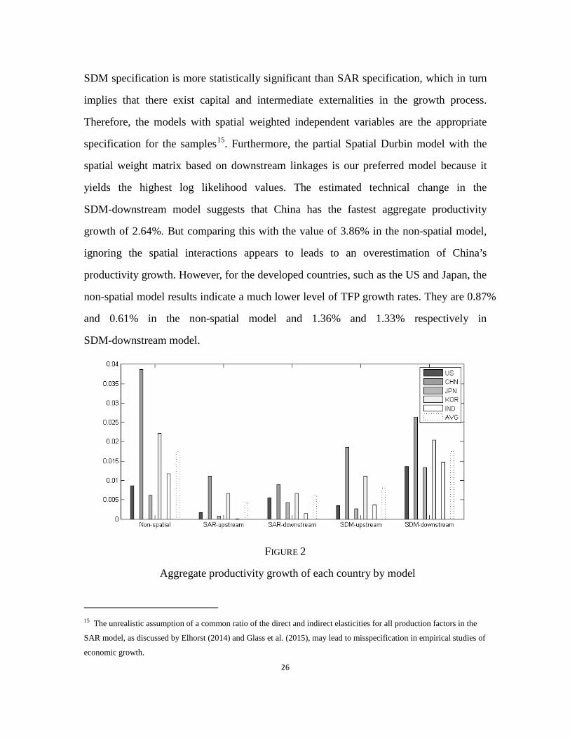
26

SDM specification is more statistically significant than SAR specification, which in turn

implies that there exist capital and intermediate externalities in the growth process.

Therefore, the models with spatial weighted independent variables are the appropriate

specification for the samples15. Furthermore, the partial Spatial Durbin model with the

spatial weight matrix based on downstream linkages is our preferred model because it

yields the highest log likelihood values. The estimated technical change in the

SDM-downstream model suggests that China has the fastest aggregate productivity

growth of 2.64%. But comparing this with the value of 3.86% in the non-spatial model,

ignoring the spatial interactions appears to leads to an overestimation of China’s

productivity growth. However, for the developed countries, such as the US and Japan, the

non-spatial model results indicate a much lower level of TFP growth rates. They are 0.87%

and 0.61% in the non-spatial model and 1.36% and 1.33% respectively in

SDM-downstream model.

FIGURE 2

Aggregate productivity growth of each country by model

15 The unrealistic assumption of a common ratio of the direct and indirect elasticities for all production factors in the

SAR model, as discussed by Elhorst (2014) and Glass et al. (2015), may lead to misspecification in empirical studies of

economic growth.

27

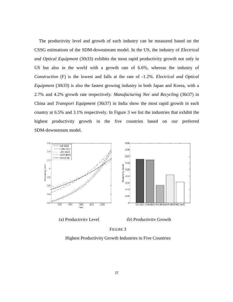
The productivity level and growth of each industry can be measured based on the

CSSG estimations of the SDM-downstream model. In the US, the industry of Electrical

and Optical Equipment (30t33) exhibits the most rapid productivity growth not only in

US but also in the world with a growth rate of 6.6%, whereas the industry of

Construction (F) is the lowest and falls at the rate of -1.2%. Electrical and Optical

Equipment (30t33) is also the fastest growing industry in both Japan and Korea, with a

2.7% and 4.2% growth rate respectively. Manufacturing Nec and Recycling (36t37) in

China and Transport Equipment (36t37) in India show the most rapid growth in each

country at 6.5% and 3.1% respectively. In Figure 3 we list the industries that exhibit the

highest productivity growth in the five countries based on our preferred

SDM-downstream model.

FIGURE 3

Highest Productivity Growth Industries in Five Countries

(a) Productivity Level (b) Productivity Growth

28

5.2 The elasticity of input factors and spatial spillovers

The coefficients of the independent variables represent the output elasticities of input

factors in a non-spatial production function setting. Whereas, when cross-section

interaction exists, the output change of one industry due to the adjustment of the factor

input should not only consider changes in the factor input itself, but also induced changes

in its neighbor’s inputs. Therefore the output elasticity for the all the industries should be

a 𝑁𝑁 × 𝑁𝑁 matrix. As suggested by LeSage and Pace (2009), we diagonalize the

coefficient of independent variables and add the local interaction from neighbor’s inputs,

then multiply the inverse matrix, (𝛪𝛪𝑁𝑁 − 𝜌𝜌𝑊𝑊)−1 , to derive the expressions for the

matrix-formed output elasticity of input factors given in Eq. (14). Hence, an elasticity in a

spatial setting includes two parts: the internal elasticity expressed by the direct effect,

which is the average along the diagonal, and external elasticity measured by the indirect

effect, which is the average of the row (or column) sums of the off-diagonal elements.

Average total output elasticity is expressed by the sum of the direct and indirect effects.

We calculate the direct, indirect and total effects. To test for the significance of these

effects, we follow the algorithms LeSage and Pace (2009) suggested by drawing

parameter estimates 1000 times based on the variance-covariance matrix of the

parameters to get the corresponding distribution of these effects, and then we compute

their means and standard deviations based on the simulation.

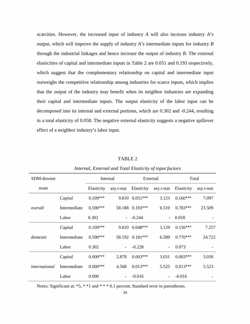
The top row of Table 2 shows the internal, external and total output elasticity of each

factor input in the SDM-downstream model. The internal elasticities of capital and

intermediate inputs are 0.109 and 0.590 respectively and both are statistically significant,

which is approximately consistent with the results in the non-spatial model. The external

elasticities reflect the spillover effects of the input factors. From the perspective of

industry production, the spillover effects are two-fold. When the factor input of industry

A is increased, the output of its neighbor, industry B, may decrease because of factor

29

scarcities. However, the increased input of industry A will also increase industry A’s

output, which will improve the supply of industry A’s intermediate inputs for industry B

through the industrial linkages and hence increase the output of industry B. The external

elasticities of capital and intermediate inputs in Table 2 are 0.051 and 0.193 respectively,

which suggest that the complementary relationship on capital and intermediate input

outweighs the competitive relationship among industries for scarce inputs, which implies

that the output of the industry may benefit when its neighbor industries are expanding

their capital and intermediate inputs. The output elasticity of the labor input can be

decomposed into its internal and external portions, which are 0.302 and -0.244, resulting

in a total elasticity of 0.058. The negative external elasticity suggests a negative spillover

effect of a neighbor industry’s labor input.

TABLE 2

Internal, External and Total Elasticity of input factors

SDM-downst

ream

Internal External Total

Elasticity asy.t-stat Elasticity asy.t-stat Elasticity asy.t-stat

Capital 0.109*** 9.810 0.051*** 3.123 0.160*** 7.097

overall Intermediate 0.590*** 58.188 0.193*** 6.510 0.783*** 23.509

Labor 0.302 - -0.244 - 0.058 -

Capital 0.109*** 9.810 0.048*** 3.129 0.156*** 7.257

domestic Intermediate 0.590*** 58.192 0.181*** 6.589 0.770*** 24.722

Labor 0.302 - -0.228 - 0.073 -

Capital 0.000*** 2.878 0.003*** 3.031 0.003*** 3.030

international Intermediate 0.000*** 4.568 0.013*** 5.525 0.013*** 5.523

Labor 0.000 - -0.016 - -0.016 -

Notes: Significant at: *5, * *1 and * * * 0.1 percent; Standard error in parentheses.

30

We next decompose the elasticities based on Eq. (18) and Eq. (19) in order to measure

the spillovers that spread among domestic and international industries separately. As

shown in the last 2 rows of Table 2, for the internal elasticity, the international part is

negligible because only a small part of the feedback component in the direct effect can be

attributed to the international linkage. From the decomposition of the external elasticity,

however, we find that international spillovers constitute about 6.5% of the external

elasticity for each of the factor inputs. Since the calculation is based on a time-invariant

specification of the spatial weight matrix in 1995, and the growth of international

intermediate trade has been much higher than the growth of world GDP since then, we

may expect an increasing trend for the international part in the overall spillover16.

5.3 Hicks-neutral technical change and spatial spillovers

One advantage of our spatial model with heterogenetic technical change is that we can

estimate the industry-specific Hicks-neutral technical change and its direct and indirect

effect in the global value chain setting. Complete empirical results of Hicks-neutral

technical change in the SDM-downstream model for all cross-sectional samples are

displayed in Table 3. The Domar-weighted aggregate of the five countries are shown in

Figure 4. The direct and indirect effects, and their decompositions into domestic and

international spillovers, are constructed from Eq. (15b) and Eq. (19). Standard errors for

the direct and indirect effects are based on simulations wherein we bootstrap 1000 times

to calculate the variance-covariance matrix for 𝛿𝛿𝑖𝑖 and other parameters in SDM model,

then follow same process as LeSage and Pace (2009) to get significance levels.

16 We estimate the model with spatial weight matrix constructed by the world input-output table of 2010. The

international spillovers constitute about 9.8% of the external elasticity of each factor inputs. The elasticity results are

given in Appendix C.

31

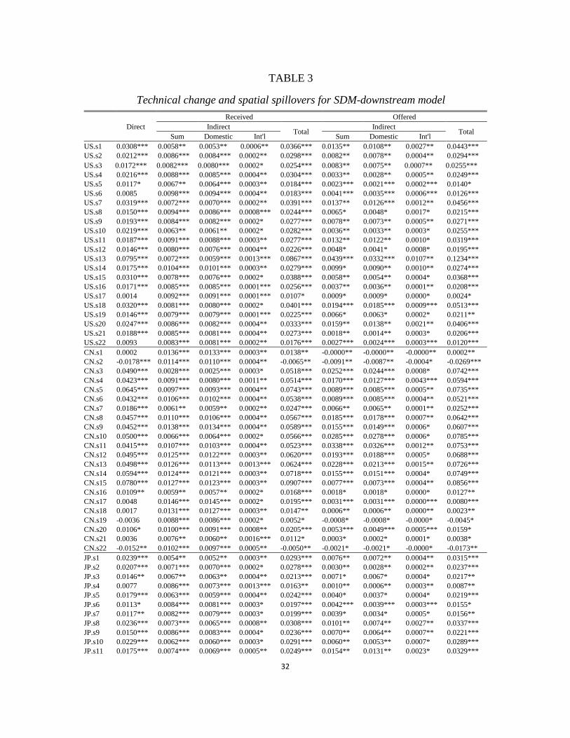
The left side of Figure 4 represents the technological growth measured by the direct

and indirect effects from the receiving perspective. The direct effect represents the

technological growth by the industry itself that mostly comes from the independent

innovation or improvement within the industry. On country level, China exhibits the most

rapid internal technological growth measured by the direct effect at 5.92%, while the

growth rates for Korea, India, Japan and US are 4.78%, 4.09%, 3.89% and 3.84%,

respectively. The indirect effects represent the Hicks-neutral technology spillovers that

industries receive through producing intermediate inputs for their user industries. The

weighted average indirect effects for China, Korea, India, US and Japan are 2.68%,

1.90%, 1.60%, 1.56% and 1.44%, respectively. The spillovers received account for 27%

to 31% of the total technological growth of the countries in our sample.

32

TABLE 3

Technical change and spatial spillovers for SDM-downstream model

Direct Received Offered

Indirect Total Indirect Total Sum Domestic Int'l Sum Domestic Int'l US.s1 0.0308*** 0.0058** 0.0053** 0.0006** 0.0366*** 0.0135** 0.0108** 0.0027** 0.0443*** US.s2 0.0212*** 0.0086*** 0.0084*** 0.0002** 0.0298*** 0.0082** 0.0078** 0.0004** 0.0294*** US.s3 0.0172*** 0.0082*** 0.0080*** 0.0002* 0.0254*** 0.0083** 0.0075** 0.0007** 0.0255*** US.s4 0.0216*** 0.0088*** 0.0085*** 0.0004** 0.0304*** 0.0033** 0.0028** 0.0005** 0.0249*** US.s5 0.0117* 0.0067** 0.0064*** 0.0003** 0.0184*** 0.0023*** 0.0021*** 0.0002*** 0.0140* US.s6 0.0085 0.0098*** 0.0094*** 0.0004** 0.0183*** 0.0041*** 0.0035*** 0.0006*** 0.0126*** US.s7 0.0319*** 0.0072*** 0.0070*** 0.0002** 0.0391*** 0.0137** 0.0126*** 0.0012** 0.0456*** US.s8 0.0150*** 0.0094*** 0.0086*** 0.0008*** 0.0244*** 0.0065* 0.0048* 0.0017* 0.0215*** US.s9 0.0193*** 0.0084*** 0.0082*** 0.0002* 0.0277*** 0.0078** 0.0073** 0.0005** 0.0271*** US.s10 0.0219*** 0.0063** 0.0061** 0.0002* 0.0282*** 0.0036** 0.0033** 0.0003* 0.0255*** US.s11 0.0187*** 0.0091*** 0.0088*** 0.0003** 0.0277*** 0.0132** 0.0122** 0.0010* 0.0319*** US.s12 0.0146*** 0.0080*** 0.0076*** 0.0004** 0.0226*** 0.0048* 0.0041* 0.0008* 0.0195*** US.s13 0.0795*** 0.0072*** 0.0059*** 0.0013*** 0.0867*** 0.0439*** 0.0332*** 0.0107** 0.1234*** US.s14 0.0175*** 0.0104*** 0.0101*** 0.0003** 0.0279*** 0.0099* 0.0090** 0.0010** 0.0274*** US.s15 0.0310*** 0.0078*** 0.0076*** 0.0002* 0.0388*** 0.0058** 0.0054** 0.0004* 0.0368*** US.s16 0.0171*** 0.0085*** 0.0085*** 0.0001*** 0.0256*** 0.0037** 0.0036** 0.0001** 0.0208*** US.s17 0.0014 0.0092*** 0.0091*** 0.0001*** 0.0107* 0.0009* 0.0009* 0.0000* 0.0024* US.s18 0.0320*** 0.0081*** 0.0080*** 0.0002* 0.0401*** 0.0194*** 0.0185*** 0.0009*** 0.0513*** US.s19 0.0146*** 0.0079*** 0.0079*** 0.0001*** 0.0225*** 0.0066* 0.0063* 0.0002* 0.0211** US.s20 0.0247*** 0.0086*** 0.0082*** 0.0004** 0.0333*** 0.0159** 0.0138** 0.0021** 0.0406*** US.s21 0.0188*** 0.0085*** 0.0081*** 0.0004** 0.0273*** 0.0018** 0.0014** 0.0003* 0.0206*** US.s22 0.0093 0.0083*** 0.0081*** 0.0002** 0.0176*** 0.0027*** 0.0024*** 0.0003*** 0.0120*** CN.s1 0.0002 0.0136*** 0.0133*** 0.0003** 0.0138** -0.0000** -0.0000** -0.0000** 0.0002** CN.s2 -0.0178*** 0.0114*** 0.0110*** 0.0004** -0.0065** -0.0091** -0.0087** -0.0004* -0.0269*** CN.s3 0.0490*** 0.0028*** 0.0025*** 0.0003* 0.0518*** 0.0252*** 0.0244*** 0.0008* 0.0742*** CN.s4 0.0423*** 0.0091*** 0.0080*** 0.0011** 0.0514*** 0.0170*** 0.0127*** 0.0043*** 0.0594*** CN.s5 0.0645*** 0.0097*** 0.0093*** 0.0004** 0.0743*** 0.0089*** 0.0085*** 0.0005** 0.0735*** CN.s6 0.0432*** 0.0106*** 0.0102*** 0.0004** 0.0538*** 0.0089*** 0.0085*** 0.0004** 0.0521*** CN.s7 0.0186*** 0.0061** 0.0059** 0.0002** 0.0247*** 0.0066** 0.0065** 0.0001** 0.0252*** CN.s8 0.0457*** 0.0110*** 0.0106*** 0.0004** 0.0567*** 0.0185*** 0.0178*** 0.0007** 0.0642*** CN.s9 0.0452*** 0.0138*** 0.0134*** 0.0004** 0.0589*** 0.0155*** 0.0149*** 0.0006* 0.0607*** CN.s10 0.0500*** 0.0066*** 0.0064*** 0.0002* 0.0566*** 0.0285*** 0.0278*** 0.0006* 0.0785*** CN.s11 0.0415*** 0.0107*** 0.0103*** 0.0004** 0.0523*** 0.0338*** 0.0326*** 0.0012** 0.0753*** CN.s12 0.0495*** 0.0125*** 0.0122*** 0.0003** 0.0620*** 0.0193*** 0.0188*** 0.0005* 0.0688*** CN.s13 0.0498*** 0.0126*** 0.0113*** 0.0013*** 0.0624*** 0.0228*** 0.0213*** 0.0015** 0.0726*** CN.s14 0.0594*** 0.0124*** 0.0121*** 0.0003** 0.0718*** 0.0155*** 0.0151*** 0.0004* 0.0749*** CN.s15 0.0780*** 0.0127*** 0.0123*** 0.0003** 0.0907*** 0.0077*** 0.0073*** 0.0004** 0.0856*** CN.s16 0.0109** 0.0059** 0.0057** 0.0002* 0.0168*** 0.0018* 0.0018* 0.0000* 0.0127** CN.s17 0.0048 0.0146*** 0.0145*** 0.0002* 0.0195*** 0.0031*** 0.0031*** 0.0000*** 0.0080*** CN.s18 0.0017 0.0131*** 0.0127*** 0.0003** 0.0147** 0.0006** 0.0006** 0.0000** 0.0023** CN.s19 -0.0036 0.0088*** 0.0086*** 0.0002* 0.0052* -0.0008* -0.0008* -0.0000* -0.0045* CN.s20 0.0106* 0.0100*** 0.0091*** 0.0008** 0.0205*** 0.0053*** 0.0049*** 0.0005*** 0.0159* CN.s21 0.0036 0.0076** 0.0060** 0.0016*** 0.0112* 0.0003* 0.0002* 0.0001* 0.0038* CN.s22 -0.0152** 0.0102*** 0.0097*** 0.0005** -0.0050** -0.0021* -0.0021* -0.0000* -0.0173** JP.s1 0.0239*** 0.0054** 0.0052** 0.0003** 0.0293*** 0.0076** 0.0072** 0.0004** 0.0315*** JP.s2 0.0207*** 0.0071*** 0.0070*** 0.0002* 0.0278*** 0.0030** 0.0028** 0.0002** 0.0237*** JP.s3 0.0146** 0.0067** 0.0063** 0.0004** 0.0213*** 0.0071* 0.0067* 0.0004* 0.0217** JP.s4 0.0077 0.0086*** 0.0073*** 0.0013*** 0.0163** 0.0010** 0.0006** 0.0003** 0.0087** JP.s5 0.0179*** 0.0063*** 0.0059*** 0.0004** 0.0242*** 0.0040* 0.0037* 0.0004* 0.0219*** JP.s6 0.0113* 0.0084*** 0.0081*** 0.0003* 0.0197*** 0.0042*** 0.0039*** 0.0003*** 0.0155* JP.s7 0.0117** 0.0082*** 0.0079*** 0.0003* 0.0199*** 0.0039* 0.0034* 0.0005* 0.0156** JP.s8 0.0236*** 0.0073*** 0.0065*** 0.0008** 0.0308*** 0.0101** 0.0074** 0.0027** 0.0337*** JP.s9 0.0150*** 0.0086*** 0.0083*** 0.0004* 0.0236*** 0.0070** 0.0064** 0.0007** 0.0221*** JP.s10 0.0229*** 0.0062*** 0.0060*** 0.0003* 0.0291*** 0.0060** 0.0053** 0.0007* 0.0289*** JP.s11 0.0175*** 0.0074*** 0.0069*** 0.0005** 0.0249*** 0.0154** 0.0131** 0.0023* 0.0329***

33

JP.s12 0.0260*** 0.0079*** 0.0072*** 0.0008** 0.0340*** 0.0087** 0.0070** 0.0017** 0.0347***

TABLE 3 (Continued )

Direct Received Offered

Indirect Total Indirect Total Sum Domestic Int'l Sum Domestic Int'l JP.s13 0.0397*** 0.0082*** 0.0064*** 0.0019*** 0.0479*** 0.0207*** 0.0151*** 0.0056** 0.0604*** JP.s14 0.0199*** 0.0087*** 0.0082*** 0.0005** 0.0286*** 0.0080* 0.0068** 0.0012* 0.0278*** JP.s15 0.0142** 0.0075*** 0.0072*** 0.0004** 0.0217*** 0.0016*** 0.0015* 0.0002* 0.0158** JP.s16 0.0311*** 0.0071*** 0.0070*** 0.0001*** 0.0382*** 0.0100** 0.0096*** 0.0004*** 0.0411*** JP.s17 0.0110** 0.0075*** 0.0072*** 0.0003** 0.0185*** 0.0120* 0.0113* 0.0008* 0.0231** JP.s18 0.0273*** 0.0071*** 0.0068*** 0.0003** 0.0344*** 0.0230** 0.0216** 0.0013* 0.0502*** JP.s19 0.0109* 0.0077*** 0.0075*** 0.0002* 0.0186*** 0.0059*** 0.0057*** 0.0002*** 0.0168* JP.s20 0.0214*** 0.0074*** 0.0071*** 0.0003** 0.0289*** 0.0112** 0.0103** 0.0009* 0.0326*** JP.s21 0.0183*** 0.0076*** 0.0073*** 0.0003** 0.0259*** 0.0019** 0.0017** 0.0002* 0.0202*** JP.s22 0.0151*** 0.0073*** 0.0071*** 0.0002* 0.0224*** 0.0034* 0.0033* 0.0001* 0.0185*** KR.s1 0.0203*** 0.0060** 0.0051** 0.0008* 0.0263*** 0.0074** 0.0072** 0.0002** 0.0277*** KR.s2 0.0490*** 0.0089*** 0.0084*** 0.0005*** 0.0579*** 0.0034*** 0.0034*** 0.0001*** 0.0524*** KR.s3 0.0169*** 0.0070** 0.0056** 0.0014** 0.0238*** 0.0060** 0.0057** 0.0003** 0.0228*** KR.s4 0.0214*** 0.0091*** 0.0042*** 0.0050*** 0.0305*** 0.0035** 0.0027** 0.0008** 0.0248*** KR.s5 0.0252*** 0.0065** 0.0056** 0.0008* 0.0317*** 0.0025** 0.0024** 0.0001* 0.0277*** KR.s6 0.0157*** 0.0085*** 0.0074*** 0.0012** 0.0242*** 0.0044** 0.0043** 0.0001** 0.0201*** KR.s7 0.0236*** 0.0090*** 0.0084*** 0.0007*** 0.0327*** 0.0107** 0.0105** 0.0003* 0.0344*** KR.s8 0.0319*** 0.0091*** 0.0070*** 0.0021** 0.0410*** 0.0129** 0.0119** 0.0010** 0.0448*** KR.s9 0.0139** 0.0105*** 0.0092*** 0.0013** 0.0244*** 0.0051* 0.0049* 0.0002* 0.0190** KR.s10 0.0283*** 0.0076*** 0.0068*** 0.0008* 0.0360*** 0.0121*** 0.0118*** 0.0003* 0.0405*** KR.s11 0.0212*** 0.0088*** 0.0073*** 0.0015** 0.0300*** 0.0134** 0.0128** 0.0006* 0.0345*** KR.s12 0.0317*** 0.0091*** 0.0070*** 0.0020** 0.0408*** 0.0094** 0.0089** 0.0005** 0.0411*** KR.s13 0.0557*** 0.0111*** 0.0052*** 0.0059*** 0.0668*** 0.0251*** 0.0228*** 0.0024** 0.0808*** KR.s14 0.0300*** 0.0104*** 0.0081*** 0.0023** 0.0404*** 0.0107** 0.0101** 0.0006* 0.0408*** KR.s15 0.0194*** 0.0080*** 0.0068*** 0.0012** 0.0275*** 0.0040** 0.0039** 0.0001* 0.0235*** KR.s16 0.0324*** 0.0073** 0.0066*** 0.0008* 0.0397*** 0.0081*** 0.0080*** 0.0001* 0.0406*** KR.s17 0.0039 0.0102*** 0.0089*** 0.0013** 0.0141** 0.0031** 0.0031** 0.0001** 0.0070** KR.s18 0.0226*** 0.0087*** 0.0074*** 0.0013** 0.0312*** 0.0061** 0.0059** 0.0002* 0.0287*** KR.s19 0.0051 0.0097*** 0.0087*** 0.0009** 0.0147** 0.0018** 0.0018** 0.0000** 0.0069** KR.s20 0.0266*** 0.0081*** 0.0063*** 0.0018** 0.0347*** 0.0147** 0.0135*** 0.0011** 0.0413*** KR.s21 0.0192*** 0.0093*** 0.0082*** 0.0011** 0.0286*** 0.0009** 0.0009** 0.0000* 0.0202*** KR.s22 -0.0003 0.0096*** 0.0086*** 0.0011** 0.0094** -0.0000** -0.0000** -0.0000** -0.0003** IN.s2 0.0233*** 0.0079*** 0.0077*** 0.0002* 0.0312*** 0.0215** 0.0213** 0.0002* 0.0448*** IN.s3 0.0136** 0.0080*** 0.0078*** 0.0002* 0.0216*** 0.0046* 0.0045* 0.0000* 0.0181** IN.s4 0.0263*** 0.0081*** 0.0079*** 0.0002** 0.0344*** 0.0092** 0.0091** 0.0001* 0.0354*** IN.s5 0.0283*** 0.0088*** 0.0083*** 0.0006** 0.0371*** 0.0081** 0.0079** 0.0002** 0.0364*** IN.s6 -0.0208*** 0.0078** 0.0076** 0.0002* -0.0130* -0.0044** -0.0044** -0.0000* -0.0252*** IN.s7 0.0174*** 0.0080*** 0.0074*** 0.0006** 0.0254*** 0.0020** 0.0020** 0.0000** 0.0195*** IN.s8 0.0075 0.0077*** 0.0076*** 0.0001*** 0.0152** 0.0040** 0.0040** 0.0000** 0.0116** IN.s9 0.0288*** 0.0084*** 0.0078*** 0.0006** 0.0372*** 0.0105*** 0.0103*** 0.0002** 0.0392*** IN.s10 0.0215*** 0.0093*** 0.0090*** 0.0004** 0.0308*** 0.0052** 0.0051** 0.0001* 0.0267*** IN.s11 0.0339*** 0.0050** 0.0047** 0.0003** 0.0389*** 0.0086** 0.0085** 0.0001** 0.0425*** IN.s12 0.0352*** 0.0074*** 0.0072*** 0.0002** 0.0426*** 0.0344*** 0.0342*** 0.0002* 0.0696*** IN.s13 0.0056 0.0106*** 0.0101*** 0.0005** 0.0162** 0.0013** 0.0013** 0.0000** 0.0069** IN.s14 0.0446*** 0.0095*** 0.0088*** 0.0007*** 0.0541*** 0.0058** 0.0058*** 0.0001** 0.0505*** IN.s15 0.0237*** 0.0093*** 0.0090*** 0.0004** 0.0330*** 0.0095** 0.0094** 0.0001* 0.0331*** IN.s16 0.0346*** 0.0104*** 0.0101*** 0.0003** 0.0449*** 0.0093** 0.0092** 0.0001** 0.0439*** IN.s17 0.0350*** 0.0070*** 0.0067*** 0.0003** 0.0420*** 0.0114*** 0.0113*** 0.0001** 0.0464*** IN.s19 0.0066 0.0084*** 0.0081*** 0.0003** 0.0150** 0.0043** 0.0043** 0.0000** 0.0109** IN.s20 0.0302*** 0.0088*** 0.0087*** 0.0001* 0.0390*** 0.0044** 0.0043** 0.0000* 0.0346*** IN.s21 0.0174*** 0.0081*** 0.0078*** 0.0003** 0.0255*** 0.0107** 0.0106** 0.0001* 0.0281*** IN.s22 0.0274*** 0.0080*** 0.0078*** 0.0002** 0.0354*** 0.0010** 0.0010** 0.0000** 0.0284***

Notes: Significant at: *5, * *1 and * * * 0.1 percent; Standard error in parentheses.

34

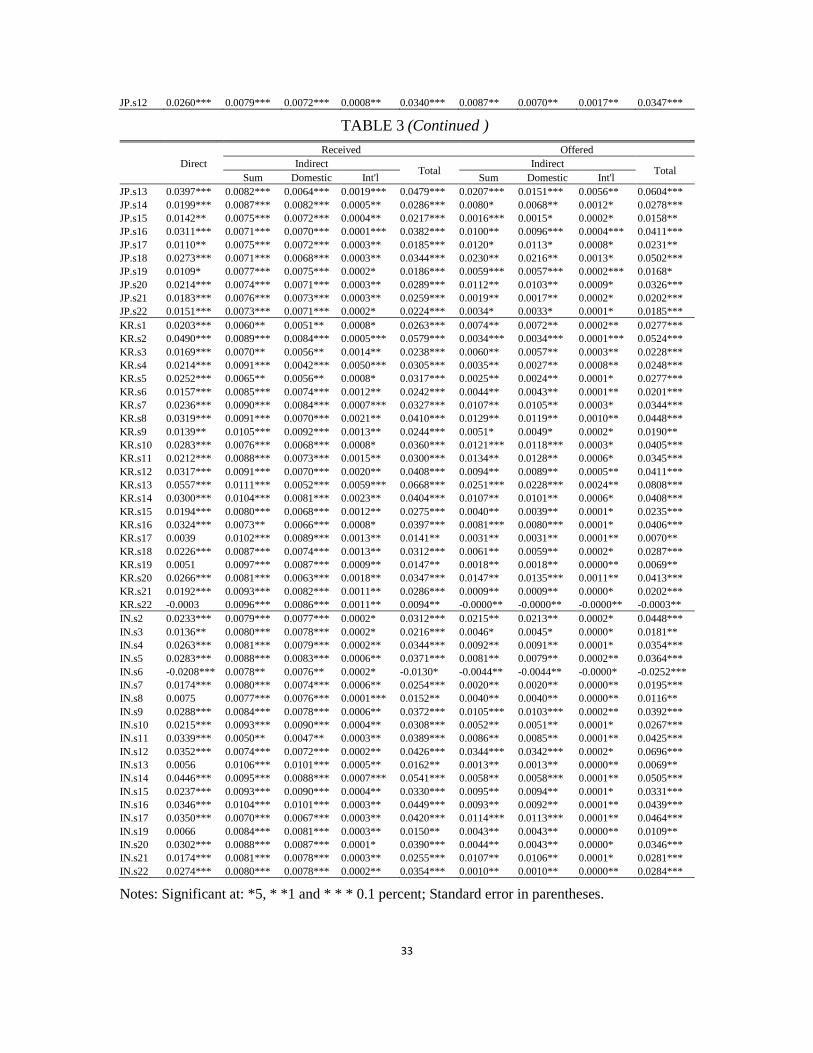
By decomposing the indirect effects into domestic and international spillovers, Korea

is found to have benefited most from international spillovers, with an international

indirect effect of 0.41%, which constitutes 21.5% of the total spillovers that Korea’s

industries received. Japan has an international effect of 0.08%, which constitutes 5.6% of

the total spillover Japan’s industries received. The international parts are relatively small

for the remaining three countries, with less than 5% in total received spillovers.

The right side of Figure 4 represents the technological growth of each country from the

offering perspective. The direct effects are comparable to values on the left side of Figure

4. The aggregated indirect effects for China, Japan, India, Korea and US are 2.72%,

2.12%, 2.09%, 1.88% and 1.79%17. However, the international spillovers that each

country offers are different from those that they receive. The US and Japan contribute the

most international spillovers with a growth impact of 2.15‰ and 1.94‰, which accounts

for 10.83% and 10.14% of their total offered spillovers. The international spillovers for

China, Korea and India are 1.41‰, 1.21‰ and 0.18‰. Our results suggest that while

China is the most rapidly growing economy in the world, the developed countries, such

as US and Japan, still contribute the most to international knowledge diffusion 18.

Combined with the results of the international spillovers received by each country, we

can find that US and Japan made the most net contributions with net international

spillovers at 1.37‰ and 1.34‰, followed by China at 0.19‰. Korea benefits most with

net international spillovers at -2.88‰.

The relatively small role for India in terms of international spillovers is mirrored by its

relatively small international indirect effect of 0.18‰, which is only 2% of its indirect

17 The summation of indirect effect received and offered are not equal because the average is weighted by the output of

the industries. 18 We calculate the technological growth components with estimates based on the 2010 input-output tables and found

China and US had become the net contributors for international knowledge diffusion. The result is given in Appendix

C.

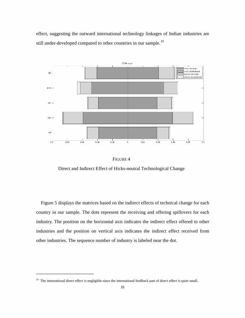
35

effect, suggesting the outward international technology linkages of Indian industries are

still under-developed compared to other countries in our sample.19

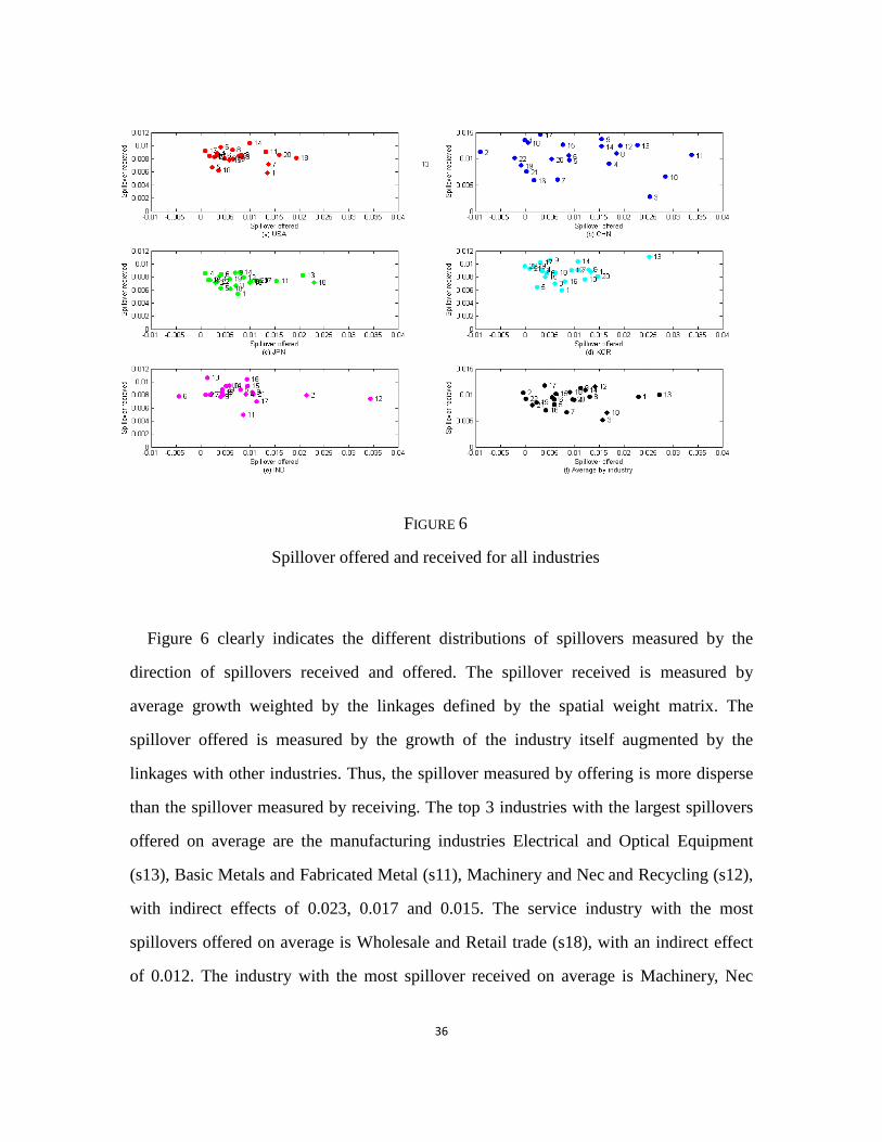
Figure 5 displays the matrices based on the indirect effects of technical change for each

country in our sample. The dots represent the receiving and offering spillovers for each

industry. The position on the horizontal axis indicates the indirect effect offered to other

industries and the position on vertical axis indicates the indirect effect received from

other industries. The sequence number of industry is labeled near the dot.

19 The international direct effect is negligible since the international feedback part of direct effect is quite small.

FIGURE 4

Direct and Indirect Effect of Hicks-neutral Technological Change

36

Figure 6 clearly indicates the different distributions of spillovers measured by the

direction of spillovers received and offered. The spillover received is measured by

average growth weighted by the linkages defined by the spatial weight matrix. The

spillover offered is measured by the growth of the industry itself augmented by the

linkages with other industries. Thus, the spillover measured by offering is more disperse

than the spillover measured by receiving. The top 3 industries with the largest spillovers

offered on average are the manufacturing industries Electrical and Optical Equipment

(s13), Basic Metals and Fabricated Metal (s11), Machinery and Nec and Recycling (s12),

with indirect effects of 0.023, 0.017 and 0.015. The service industry with the most

spillovers offered on average is Wholesale and Retail trade (s18), with an indirect effect

of 0.012. The industry with the most spillover received on average is Machinery, Nec

FIGURE 6

Spillover offered and received for all industries

37

(s12), with an indirect effect of 0.014. The other industries are relatively concentrated in

distribution.

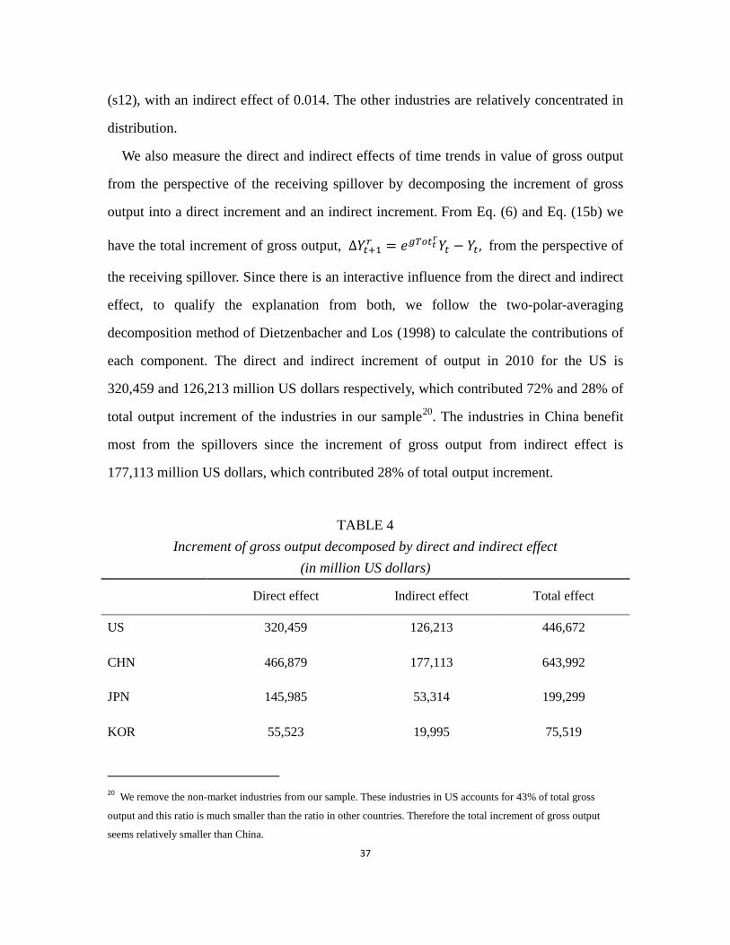
We also measure the direct and indirect effects of time trends in value of gross output

from the perspective of the receiving spillover by decomposing the increment of gross

output into a direct increment and an indirect increment. From Eq. (6) and Eq. (15b) we

have the total increment of gross output, ∆𝑌𝑌𝑡𝑡+1𝐷𝐷 = 𝑒𝑒𝑔𝑔𝑇𝑇𝑇𝑇𝑡𝑡𝑡𝑡𝑟𝑟𝑌𝑌𝑡𝑡 − 𝑌𝑌𝑡𝑡, from the perspective of

the receiving spillover. Since there is an interactive influence from the direct and indirect

effect, to qualify the explanation from both, we follow the two-polar-averaging

decomposition method of Dietzenbacher and Los (1998) to calculate the contributions of

each component. The direct and indirect increment of output in 2010 for the US is

320,459 and 126,213 million US dollars respectively, which contributed 72% and 28% of

total output increment of the industries in our sample20. The industries in China benefit

most from the spillovers since the increment of gross output from indirect effect is

177,113 million US dollars, which contributed 28% of total output increment.

TABLE 4 Increment of gross output decomposed by direct and indirect effect

(in million US dollars)

Direct effect Indirect effect Total effect

US 320,459 126,213 446,672

CHN 466,879 177,113 643,992

JPN 145,985 53,314 199,299

KOR 55,523 19,995 75,519

20 We remove the non-market industries from our sample. These industries in US accounts for 43% of total gross

output and this ratio is much smaller than the ratio in other countries. Therefore the total increment of gross output

seems relatively smaller than China.

38

IND 51,531 19,798 71,329

5.4 Productivity level and change for selected industries: electrical and optical

equipment

The information and communication technology (ICT) industry is one of the fastest

growing industries in the world and highlights the increasingly important role of the

global production system in the past 30 years. Jorgenson et al. (2012) note the important

role of ICT-producing industries, including software and hardware manufacturing and

services, and they found a substantial contribution of these industries to economic growth.

Due to the importance of ICT as a main industry in which innovation takes places and

provides an engine for long-run growth in an economy, we next examine the Electrical

and Optical Equipment industry to show the performance of the ICT industry in the five

countries we study and the way in which spillovers are diffused through domestic and

international supply chains.

39

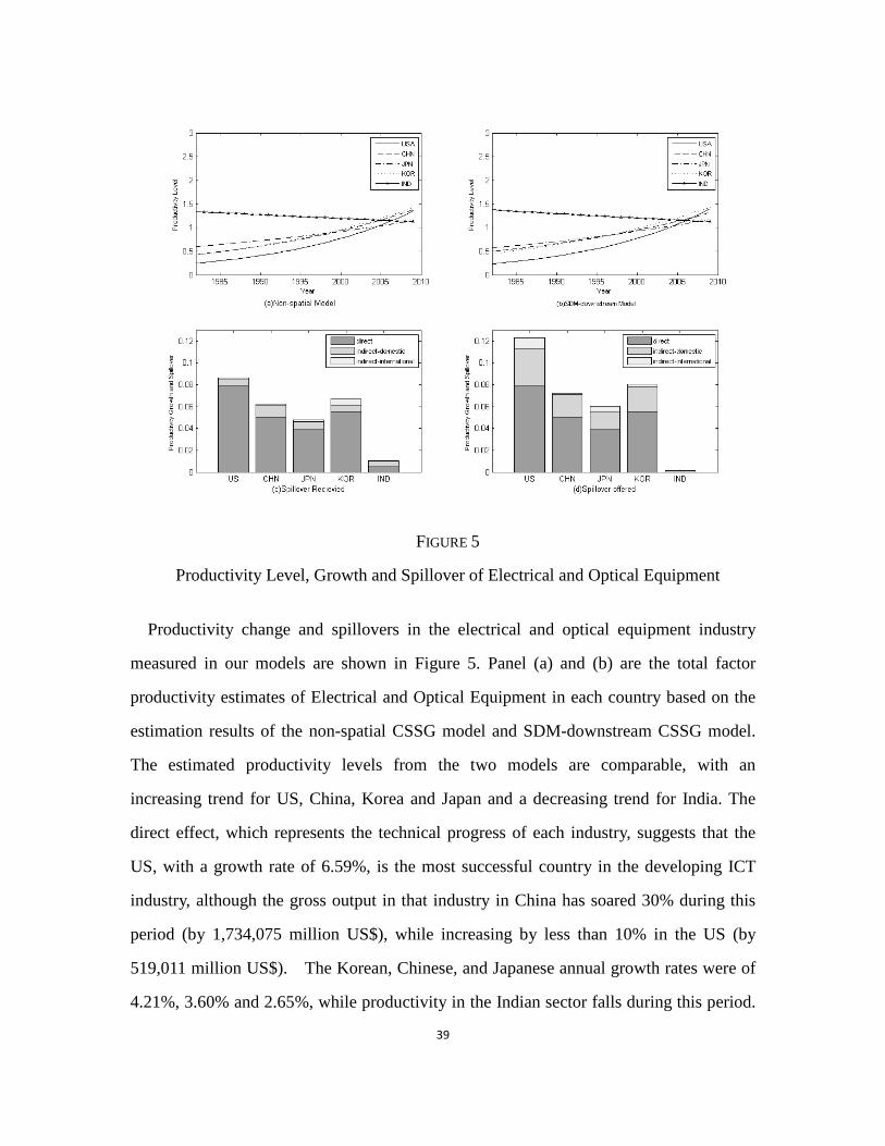
Productivity change and spillovers in the electrical and optical equipment industry

measured in our models are shown in Figure 5. Panel (a) and (b) are the total factor

productivity estimates of Electrical and Optical Equipment in each country based on the

estimation results of the non-spatial CSSG model and SDM-downstream CSSG model.

The estimated productivity levels from the two models are comparable, with an

increasing trend for US, China, Korea and Japan and a decreasing trend for India. The

direct effect, which represents the technical progress of each industry, suggests that the

US, with a growth rate of 6.59%, is the most successful country in the developing ICT

industry, although the gross output in that industry in China has soared 30% during this

period (by 1,734,075 million US$), while increasing by less than 10% in the US (by

519,011 million US$). The Korean, Chinese, and Japanese annual growth rates were of

4.21%, 3.60% and 2.65%, while productivity in the Indian sector falls during this period.

FIGURE 5

Productivity Level, Growth and Spillover of Electrical and Optical Equipment

40

The gross output of electrical and optical equipment industry in India in 2010 is $72,824

million US$, which is only 4.2% of the gross output in China, suggesting a large gap in

scale exists with other countries in our sample.

The technological spillovers offered and received can help us understand the role of an

industry in technological diffusion within the global value chain. Panel (c) and (d) of

Figure 5 provide more detailed comparisons for productivity growth spillovers from the

perspective of receiving and offering. In panel (c), the estimates of spillovers received

show that China benefits most from the production network with the indirect effect of

1.26%. However, the domestic indirect effect of China is 1.13%, indicating the spillovers

mostly are coming from the domestic industrial linkages within China. The ICT of Korea

is the industry that absorbs the largest international spillover with an international indirect

effect of 0.59%.

As shown in panel (d), the spillover of productivity growth offered by US Electrical

and Optical Equipment is 4.39%, which is the highest of all industries in our sample,

suggesting that the US ICT industry is in the position of an innovation hub in the global

value chain. Korea, China and Japan follow in descending order with indirect effects of

2.51%, 2.28% and 2.07%. Compared with the sample average indirect effect of 0.86%,

ICT in these countries seems to be an important engine for regional economic

development. The Electrical and Optical Equipment sector in the US also has the highest

international growth spillover at 1.07%, followed by Japan, Korea and China at 0.56%,

0.24% and 0.15%, respectively. Therefore, although China could be thought of as

representative of a developing country while OECD member Korea, representing NIEs,

have the fastest growth measured by output of ICT, the developed countries such as the

US and Japan still have the largest contributors measured by the productivity growth

spillover offered.

41

6 Conclusion

In this paper, we develop a growth model which allows for technological interdependence

on an industry-level with heterogeneous productivity growth in the GVCs. The World

Input-output tables are used to construct the spatial weight matrix, which describes the

spatial linkages between any pair of industries. We also propose a method to measure

technology spillovers by each factor input as well as Hicks-neutral technical change.

These spillovers are then decomposed into a domestic and international effect by

separating out the local multipliers from the global multiplier of the spatial effect. We

estimate the model using non-spatial, SAR and SDM specifications.

The SDM specification is preferred over the SAR specification based on standard

statistical criteria. Results from the SDM-downstream model suggest that the internal

elasticities of factor inputs measured by direct effects are comparable to those from the

non-spatial model. However, with the spatial model we are able to estimate the indirect

effect, and we found negative external elasticities for capital and labor input and a

positive external elasticity for the intermediate input. The international indirect effect

accounts for about 6.5% of the external elasticity for each factor. The Domar-weighted

direct technical change growth rate for China, Korea, India, the US and Japan is

estimated to be 2.64%, 2.04%, 1.75%, 1.36% and 1.33%, respectively. The spillovers

received account for 27% to 31% of their total technological growth and its international

portion varies across the countries, with the highest, Korea, at 22% and lowest, India, at

3.5%. The developed countries such as US and Japan are the highest in net international

spillovers offered. The important Electrical and Optical Equipment sector of the US has

the fastest productivity growth and offers the most spillovers in our sample, although

China has predominance in scale in this industry.

Our paper also speaks to anxieties felt by both rich and poor countries as trade and

supply chains become increasingly global. Developed countries worry that technology is

42

imitated by developing countries, which may shake their dominate position in global

value chain and induce a series of problems such as industry hollowing-out and

unemployment. Developing countries worry that they are locked in low value added

activities of GVCs and have no limited options to be engaged in higher value-added

activities such as design, R&D and marketing. Our results suggest that China, as a

representative of a developing country, has experienced high productivity growth in the

globalization, but the spillovers received are mostly from domestic linkages, which may

benefit from the great varieties of industrial category in China. The international

spillovers are more likely to occur between countries at similar stages of development.

Further research oriented towards developing a spatial weight matrix that may better

depict the network of knowledge transfers among industries and estimation techniques

for time-varying social-economic spatial weight matrix with the problem of endogeneity

resolved is under way. These may allow us to better uncover the mechanism of

technology interaction among countries and sectors within them and provide more

accurate measurements of the dynamic spillover process.

43

References

Ackerberg, D.A., Caves, K. and Frazer, G., 2015. Identification properties of recent production function estimators. Econometrica, 83(6), pp.2411-2451.

Acemoglu, D., Akcigit, U. and Kerr, W., 2016. Networks and the macroeconomy: an empirical exploration. NBER Macroeconomics Annual, 30(1), pp.276–335.

Arbia, G., Battisti, M. and Di Vaio, G., 2010. Institutions and geography: Empirical test of spatial growth models for European regions. Economic modelling, 27(1), pp.12 -21.

Brock, W.A. and Durlauf, S.N., 2001. What have we learned from a decade of empirical research on growth? Growth empirics and reality. The World Bank Economic Review, 15(2), pp.229-272.

Canova, F., 2004. Testing for convergence clubs in income per capita: a predictive density approach. International Economic Review, 45(1), pp.49-77.

Case, A.C., Rosen, H.S. and Hines Jr, J.R., 1993. Budget spillovers and fiscal policy interdependence: Evidence from the states. Journal of public economics, 52(3), pp.285-307.

Carvalho, V.M, and Tahbaz-Salehi, A., 2019. Production networks: A primer. Annual Review of Economics, 11, pp.635-663.

Caves, R.E. and Caves, R.E., 1996. Multinational enterprise and economic analysis. Cambridge university press.

Coe, D.T. and Helpman, E., 1995. International R&D spillovers. European economic review, 39(5), pp.859-887.

Cohen, J.P. and Paul, C.J.M., 2004. Public infrastructure investment, interstate spatial spillovers, and manufacturing costs. Review of Economics and Statistics, 86(2), pp.551-560.

Cornwell, C., Schmidt, P. and Sickles, R.C., 1990. Production frontiers with cross-sectional and time-series variation in efficiency levels. Journal of econometrics, 46(1-2), pp.185-200.

44

Desdoigts, A., 1999. Patterns of economic development and the formation of clubs. Journal of economic growth, 4(3), pp.305-330.

Dietzenbacher, E. and Los, B., 1998. Structural decomposition techniques: sense and sensitivity. Economic Systems Research, 10(4), pp.307-324.

Domar, E.D., 1961. On the Measurement of Technological Change. Economic Journal 71(284), pp.709-729.

Durlauf S.N., 2000. Econometric analysis and the study of economic growth: a skeptical perspective. In Macroeconomics and the Real World, Backhouse R. and Salanti A. (eds). Oxford University Press: Oxford; 249 – 262.

Durlauf, S.N., 2001. Manifesto for a growth econometrics. Journal of Econometrics, 100(1), pp.65-69.

Durlauf, S.N., Kourtellos, A. and Minkin, A., 2001. The local Solow growth model. European Economic Review, 45(4-6), pp.928-940.

Durlauf, S.N. and Quah, D.T., 1999. The new empirics of economic growth. Handbook of Macroeconomics, Taylor, J. and Woodford, M. (eds). Elsevier: Amsterdam; 235 – 308.

Elhorst, J.P., 2001. Dynamic models in space and time. Geographical Analysis, 33(2), pp.119-140.

Elhorst, J.P., 2014. Spatial econometrics: from cross-sectional data to spatial panels (Vol. 479, p. 480). Heidelberg: Springer.

Eaton, J. and Kortum, S., 1996. Trade in ideas Patenting and productivity in the OECD. Journal of international Economics, 40(3-4), pp.251-278.

Ertur, C. and Koch, W., 2007. Growth, technological interdependence and spatial externalities: theory and evidence. Journal of applied econometrics, 22(6), pp.1033-1062.

Ertur, C. and Koch, W., 2011. A contribution to the theory and empirics of Schumpeterian growth with worldwide interactions. Journal of Economic Growth, 16(3), p.215.

Fingleton, B., 2008. Competing models of global dynamics: evidence from panel models with spatially correlated error components. Economic Modelling, 25(3), pp.542-558.

45

Fingleton, B. and López‐Bazo, E., 2006. Empirical growth models with spatial effects. Papers in regional science, 85(2), pp.177-198.

Glass, A.J., Kenjegalieva, K. and Sickles, R.C., 2015. Returns to scale and curvature in the presence of spillovers: evidence from European countries. Oxford Economic Papers, 68(1), pp.40-63.

Han, J., 2016. Essays on treatments of cross-section dependence in panel data models, unpublished PhD dissertation, Houston: Rice University,.

Han, J., Sickles, R.C., 2019. Estimation of Industry-level Productivity with Cross-sectional Dependence by Using Spatial Analysis, Working Papers 19-002, Rice University, Department of Economics.

Ho, C.Y., Wang, W. and Yu, J., 2013. Growth spillover through trade: A spatial dynamic panel data approach. Economics Letters, 120(3), pp.450-453.

Hulten, C.R., 1978. Growth Accounting with intermediate inputs. Review of Economic Studies, 45(3), pp.511-518.

Johnson, R.C. and Noguera, G., 2012. Accounting for intermediates: Production sharing and trade in value added. Journal of international Economics, 86(2), pp.224-236.

Jorgenson, D.W., Ho, M.S. and Samuels, J.D., 2012. A prototype industry-level production account for the United States, 1947-2010. Presentation to the Final World Input-Output Database Conference, Groningen, the Netherlands.

Keller, W., 2002. Geographic localization of international technology diffusion. American Economic Review, 92(1), pp.120-142.

Koopman, R., Wang, Z. and Wei, S.J., 2012. Estimating domestic content in exports when processing trade is pervasive. Journal of development economics, 99(1), pp.178-189.

Koopman, R., Wang, Z. and Wei, S.J., 2014. Tracing value-added and double counting in gross exports. American Economic Review, 104(2), pp.459-94.

LeSage, J. and Pace, R.K., 2009. Introduction to spatial econometrics. Chapman and Hall/CRC.

OECD, 2001. Productivity Measuring-Measurement of aggregate and industry-level productivity growth. Organisation for Economic Co-operation and Development.

46

Park, B.U., Sickles, R.C. and Simar, L., 2003. Semiparametric-efficient estimation of AR (1) panel data models. Journal of Econometrics, 117(2), pp.279-309.

Park, B.U., Sickles, R.C. and Simar, L., 2007. Semiparametric efficient estimation of dynamic panel data models. Journal of Econometrics, 136(1), pp.281-301.

Sickles, R.C. and Zelenyuk, V., 2019. The Measurement of Productivity and Efficiency: Theory and Practice. New York: Cambridge University Press.

Solow, R.M., 1956. A contribution to the theory of economic growth. The quarterly journal of economics, 70(1), pp.65-94.

Solow, R.M., 1957. Technical change and the aggregate production function. The review of Economics and Statistics, 39(3), pp.312-320.

Swan, T.W., 1956. Economic growth and capital accumulation. Economic record, 32(2), pp.334-361.

Timmer, M.P., Erumban, A.A., Los, B., Stehrer, R. and De Vries, G.J., 2014. Slicing up global value chains. Journal of economic perspectives, 28(2), pp.99-118.

Timmer, M. P., and Ye, X., Productivity and Substitution Patterns in Global Value Chains. In The Oxford Handbook of Productivity Analysis, Chapter 21. New York: Oxford University Press, 2017.

World Bank, OECD, IDE-JETRO, UIBE and WTO, Global Value Chain Development Report, Washington DC, 2017.

Wu, H.X. and Ito, K., 2015. Reconstructing China's Supply-Use and Input-Output Tables in Time Series , RIETI Discussion Papers , 15-E-004.

Wu, H.X., 2015. Constructing China's Net Capital and Measuring Capital Services in China, 1980-2010 , RIETI Discussion Papers , 15-E-006.

Wu, H.X., Yue, X. and Zhang, G. 2015. Constructing Annual Employment and Compensation Matrices and Measuring Labor Input in China , RIETI Discussion Papers , 15-E-005.

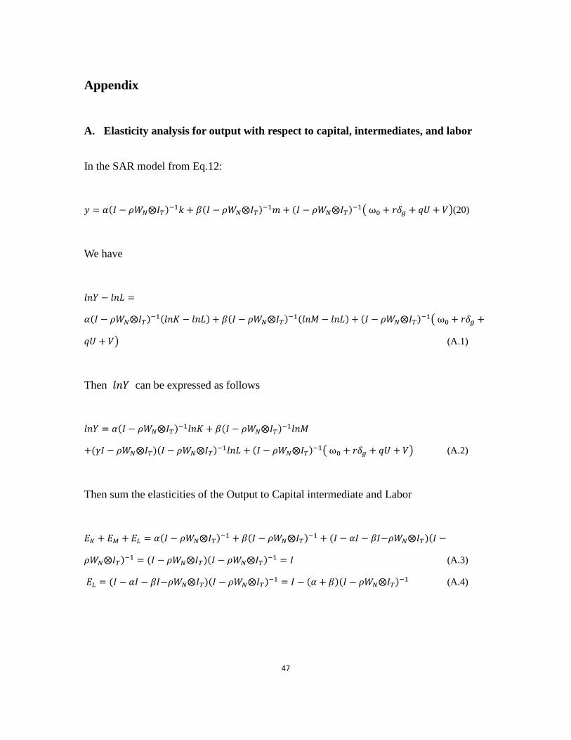
47

Appendix

A. Elasticity analysis for output with respect to capital, intermediates, and labor

In the SAR model from Eq.12:

𝑦𝑦 = 𝛼𝛼(𝛪𝛪 − 𝜌𝜌𝑊𝑊𝑁𝑁⨂𝐼𝐼𝑇𝑇)−1𝑘𝑘 + 𝛽𝛽(𝛪𝛪 − 𝜌𝜌𝑊𝑊𝑁𝑁⨂𝐼𝐼𝑇𝑇)−1𝑚𝑚 + (𝛪𝛪 − 𝜌𝜌𝑊𝑊𝑁𝑁⨂𝐼𝐼𝑇𝑇)−1 ω0 + 𝑟𝑟𝛿𝛿𝑔𝑔 + 𝑞𝑞𝑞𝑞 + 𝑉𝑉(20)

We have

𝑙𝑙𝑔𝑔𝑌𝑌 − 𝑙𝑙𝑔𝑔𝐿𝐿 =

𝛼𝛼(𝛪𝛪 − 𝜌𝜌𝑊𝑊𝑁𝑁⨂𝐼𝐼𝑇𝑇)−1(𝑙𝑙𝑔𝑔𝐾𝐾 − 𝑙𝑙𝑔𝑔𝐿𝐿) + 𝛽𝛽(𝛪𝛪 − 𝜌𝜌𝑊𝑊𝑁𝑁⨂𝐼𝐼𝑇𝑇)−1(𝑙𝑙𝑔𝑔𝑀𝑀 − 𝑙𝑙𝑔𝑔𝐿𝐿) + (𝛪𝛪 − 𝜌𝜌𝑊𝑊𝑁𝑁⨂𝐼𝐼𝑇𝑇)−1 ω0 + 𝑟𝑟𝛿𝛿𝑔𝑔 +

𝑞𝑞𝑞𝑞 + 𝑉𝑉 (A.1)

Then 𝑙𝑙𝑔𝑔𝑌𝑌 can be expressed as follows

𝑙𝑙𝑔𝑔𝑌𝑌 = 𝛼𝛼(𝛪𝛪 − 𝜌𝜌𝑊𝑊𝑁𝑁⨂𝐼𝐼𝑇𝑇)−1𝑙𝑙𝑔𝑔𝐾𝐾 + 𝛽𝛽(𝛪𝛪 − 𝜌𝜌𝑊𝑊𝑁𝑁⨂𝐼𝐼𝑇𝑇)−1𝑙𝑙𝑔𝑔𝑀𝑀

+(𝛾𝛾𝛪𝛪 − 𝜌𝜌𝑊𝑊𝑁𝑁⨂𝐼𝐼𝑇𝑇)(𝛪𝛪 − 𝜌𝜌𝑊𝑊𝑁𝑁⨂𝐼𝐼𝑇𝑇)−1𝑙𝑙𝑔𝑔𝐿𝐿 + (𝛪𝛪 − 𝜌𝜌𝑊𝑊𝑁𝑁⨂𝐼𝐼𝑇𝑇)−1 ω0 + 𝑟𝑟𝛿𝛿𝑔𝑔 + 𝑞𝑞𝑞𝑞 + 𝑉𝑉 (A.2)

Then sum the elasticities of the Output to Capital intermediate and Labor

𝐸𝐸𝐾𝐾 + 𝐸𝐸𝑀𝑀 + 𝐸𝐸𝐿𝐿 = 𝛼𝛼(𝛪𝛪 − 𝜌𝜌𝑊𝑊𝑁𝑁⨂𝐼𝐼𝑇𝑇)−1 + 𝛽𝛽(𝛪𝛪 − 𝜌𝜌𝑊𝑊𝑁𝑁⨂𝐼𝐼𝑇𝑇)−1 + (𝛪𝛪 − 𝛼𝛼𝛪𝛪 − 𝛽𝛽𝛪𝛪−𝜌𝜌𝑊𝑊𝑁𝑁⨂𝐼𝐼𝑇𝑇)(𝛪𝛪 −

𝜌𝜌𝑊𝑊𝑁𝑁⨂𝐼𝐼𝑇𝑇)−1 = (𝛪𝛪 − 𝜌𝜌𝑊𝑊𝑁𝑁⨂𝐼𝐼𝑇𝑇)(𝛪𝛪 − 𝜌𝜌𝑊𝑊𝑁𝑁⨂𝐼𝐼𝑇𝑇)−1 = 𝛪𝛪 (A.3)

𝐸𝐸𝐿𝐿 = (𝛪𝛪 − 𝛼𝛼𝛪𝛪 − 𝛽𝛽𝛪𝛪−𝜌𝜌𝑊𝑊𝑁𝑁⨂𝐼𝐼𝑇𝑇)(𝛪𝛪 − 𝜌𝜌𝑊𝑊𝑁𝑁⨂𝐼𝐼𝑇𝑇)−1 = 𝛪𝛪 − (𝛼𝛼 + 𝛽𝛽)(𝛪𝛪 − 𝜌𝜌𝑊𝑊𝑁𝑁⨂𝐼𝐼𝑇𝑇)−1 (A.4)

48

The constant return to scale assumptions still hold to the industries as an aggregate in

SAR model, but not hold for individual industries if the effects from the neighbor

industries were considered.

In the SDM model from Eq.13:

𝑦𝑦 = (𝛪𝛪 − 𝜌𝜌𝑊𝑊𝑁𝑁⨂𝐼𝐼𝑇𝑇)−1[𝛼𝛼 + (𝜙𝜙 − 𝜌𝜌𝛼𝛼)𝑊𝑊𝑁𝑁⨂𝐼𝐼𝑇𝑇]𝑘𝑘 + (𝛪𝛪 − 𝜌𝜌𝑊𝑊𝑁𝑁⨂𝐼𝐼𝑇𝑇)−1[𝛽𝛽 + (𝜑𝜑 − 𝜌𝜌𝛽𝛽)𝑊𝑊𝑁𝑁⨂𝐼𝐼𝑇𝑇]𝑚𝑚

+(𝛪𝛪 − 𝜌𝜌𝑊𝑊𝑁𝑁⨂𝐼𝐼𝑇𝑇)−1 ω0 + 𝑟𝑟𝛿𝛿𝑔𝑔 + 𝑞𝑞𝑞𝑞 + 𝑉𝑉 (A.5)

We have

𝑙𝑙𝑔𝑔𝑌𝑌 − 𝑙𝑙𝑔𝑔𝐿𝐿 = (𝛪𝛪 − 𝜌𝜌𝑊𝑊𝑁𝑁⨂𝐼𝐼𝑇𝑇)−1[𝛼𝛼𝐼𝐼 + (𝜙𝜙 − 𝜌𝜌𝛼𝛼)𝑊𝑊𝑁𝑁⨂𝐼𝐼𝑇𝑇](𝑙𝑙𝑔𝑔𝐾𝐾 − 𝑙𝑙𝑔𝑔𝐿𝐿) + (𝛪𝛪 − 𝜌𝜌𝑊𝑊𝑁𝑁⨂𝐼𝐼𝑇𝑇)−1[𝛽𝛽𝐼𝐼 +

(𝜑𝜑 − 𝜌𝜌𝛽𝛽)𝑊𝑊𝑁𝑁⨂𝐼𝐼𝑇𝑇](𝑙𝑙𝑔𝑔𝑀𝑀 − 𝑙𝑙𝑔𝑔𝐿𝐿) + (𝛪𝛪 − 𝜌𝜌𝑊𝑊𝑁𝑁⨂𝐼𝐼𝑇𝑇)−1 ω0 + 𝑟𝑟𝛿𝛿𝑔𝑔 + 𝑞𝑞𝑞𝑞 + 𝑉𝑉 (A.6)

Then we can get the expression of 𝑙𝑙𝑔𝑔𝑌𝑌

𝑙𝑙𝑔𝑔𝑌𝑌 =

(𝛪𝛪 − 𝜌𝜌𝑊𝑊𝑁𝑁⨂𝐼𝐼𝑇𝑇)−1[𝛼𝛼𝐼𝐼 + (𝜙𝜙 − 𝜌𝜌𝛼𝛼)𝑊𝑊𝑁𝑁⨂𝐼𝐼𝑇𝑇]𝑙𝑙𝑔𝑔𝐾𝐾 + (𝛪𝛪 − 𝜌𝜌𝑊𝑊𝑁𝑁⨂𝐼𝐼𝑇𝑇)−1[𝛽𝛽𝐼𝐼 + (𝜑𝜑 − 𝜌𝜌𝛽𝛽)𝑊𝑊𝑁𝑁⨂𝐼𝐼𝑇𝑇]𝑙𝑙𝑔𝑔𝑀𝑀 +

[𝛾𝛾 − (𝜙𝜙 + 𝜑𝜑)𝑊𝑊𝑁𝑁(𝛪𝛪 − 𝜌𝜌𝑊𝑊𝑁𝑁⨂𝐼𝐼𝑇𝑇)−1]𝑙𝑙𝑔𝑔𝐿𝐿 + (𝛪𝛪 − 𝜌𝜌𝑊𝑊𝑁𝑁⨂𝐼𝐼𝑇𝑇)−1 ω0 + 𝑟𝑟𝛿𝛿𝑔𝑔 + 𝑞𝑞𝑞𝑞 + 𝑉𝑉 (A.7)

Then summing the elasticities of the Output to capital intermediate and labor we can still

get the constant return to scale result.

𝐸𝐸𝐾𝐾 + 𝐸𝐸𝑀𝑀 + 𝐸𝐸𝐿𝐿 = (𝛪𝛪 − 𝜌𝜌𝑊𝑊𝑁𝑁⨂𝐼𝐼𝑇𝑇)−1[𝛼𝛼𝐼𝐼 + (𝜙𝜙 − 𝜌𝜌𝛼𝛼)𝑊𝑊𝑁𝑁⨂𝐼𝐼𝑇𝑇] + (𝛪𝛪 − 𝜌𝜌𝑊𝑊𝑁𝑁⨂𝐼𝐼𝑇𝑇)−1[𝛽𝛽𝐼𝐼 + (𝜑𝜑 −

𝜌𝜌𝛽𝛽)𝑊𝑊𝑁𝑁⨂𝐼𝐼𝑇𝑇] + (𝛪𝛪 − 𝜌𝜌𝑊𝑊𝑁𝑁⨂𝐼𝐼𝑇𝑇)−1[𝛾𝛾𝐼𝐼 + (−𝜙𝜙 − 𝜑𝜑 + 𝜌𝜌𝛾𝛾)𝑊𝑊𝑁𝑁⨂𝐼𝐼𝑇𝑇] = [𝛼𝛼𝐼𝐼 + (𝜙𝜙 − 𝜌𝜌𝛼𝛼)𝑊𝑊𝑁𝑁⨂𝐼𝐼𝑇𝑇 + 𝛽𝛽𝐼𝐼 +

(𝜑𝜑 − 𝜌𝜌𝛽𝛽)𝑊𝑊𝑁𝑁⨂𝐼𝐼𝑇𝑇 + 𝛾𝛾𝐼𝐼 − 𝜌𝜌𝛾𝛾𝑊𝑊𝑁𝑁⨂𝐼𝐼𝑇𝑇)− (𝜙𝜙 + 𝜑𝜑)𝑊𝑊𝑁𝑁⨂𝐼𝐼𝑇𝑇](𝛪𝛪 − 𝜌𝜌𝑊𝑊𝑁𝑁⨂𝐼𝐼𝑇𝑇)−1

49

= [(𝛼𝛼 + 𝛽𝛽 + 𝛾𝛾)𝐼𝐼 + (𝜙𝜙 − 𝜌𝜌𝛼𝛼 + 𝜑𝜑 − 𝜌𝜌𝛽𝛽 − 𝜌𝜌𝛾𝛾 − 𝜙𝜙 − 𝜑𝜑)𝑊𝑊𝑁𝑁⨂𝐼𝐼𝑇𝑇](𝛪𝛪 − 𝜌𝜌𝑊𝑊𝑁𝑁⨂𝐼𝐼𝑇𝑇)−1 =

[𝐼𝐼 − 𝜌𝜌𝑊𝑊𝑁𝑁⨂𝐼𝐼𝑇𝑇](𝛪𝛪 − 𝜌𝜌𝑊𝑊𝑁𝑁⨂𝐼𝐼𝑇𝑇)−1 = 𝛪𝛪 (A.8)

B. Detailed derivation of estimation procedure

The Quasi-Maximum Likelihood Estimator for ρ and its implementation are

developed in the following way. Let 2( , , , )vψ β γ ρ σ ′= . The log-likelihood function of Eq.

(7) is:

2

2

21 1 1

log ( , ; ) log(2 ) log | |2

1 ,2

i v N

N T N

it ij jt it i t ii t jv

NTL y T I W

y w y X Z R

ψ δ πσ ρ

ρ β γ δσ = = =

= − + −

′ ′ ′− − − − −

∑∑ ∑

(B.1)

The first order condition of maximizing Eq. (B.1) with respect to iδ is

21 1 1

log 1 0.N T N

t it ij jt it i t ii t ji v

L R y w y X Z Rρ β γ δδ σ = = =

∂ ′ ′ ′= − − − − = ∂

∑∑ ∑ (B.2)

By solving for (B.2), we can obtain

1

1

ˆ ( ) .N

i t t t it ij jt it ij

R R R y w y X Zδ ρ β γ−

=

′ ′ ′= − − −

∑ (B.3)

Substituting (B.3) into the log-likelihood function (B.1), we obtain the concentrated

likelihood function

2 22

1log ( ; , , ) log(2 ) log | | ,2 2v v N

v

NTL y T I W V Vβ ρ σ πσ ρσ

′= − + − − (B.4)

where ( )Q Q N T QV M y M W I y M Xρ β= − ⊗ − , and 1( ' ) 'Q NTM I Q Q Q Q−= − .

50

Within Estimator

Assuming that T L≥ , the projections onto the column space of Q and the null space of

Q are denoted by 1( )QP Q Q Q′− ′= and Q NT QM I P= − , respectively21. Suppose that the

true value of ρ is known, and is ρ∗ . Pre-multiplying by QM , we have the

within-transformed model

( ) .Q Q N T QM y M W I y M X Vρ β∗= ⊗ + +

(B.5)

Estimates of ( )β ρ∗ and 2 ( )vσ ρ∗ are derived by

1

2

ˆ ( ) ( ) ( ( ) ),1ˆ ( ) ( ) ),

( )

W Q Q N T

v

X M X X M y W I y

eN T L K

β ρ ρ

σ ρ ρ

∗ − ∗

∗ ∗ ′∗

′ ′= − ⊗

=− −

(B.6-B.7)

respectively, where ˆ( ) ( ) ( )N T We y W I y Xρ ρ β ρ∗ ∗ ∗= − ⊗ − . By substituting the closed

form solutions for the parameters ( )β ρ∗ and 2 ( )vσ ρ∗ into Eq. (B.4), we can concentrate

out β and 2vσ , and the concentrated log-likelihood function with single parameter ρ

takes the form:

[ ]log ( ; ) log ( ) ( ) log | |,2 N

NTL y C e e T I Wρ ρ ρ ρ′= − + −

(B.8)

21 Q needs to be a full column rank matrix for estimation of the individual 'i sδ .

51

where C is a constant term that is not a function of ρ . By maximizing the concentrated

log-likelihood function Eq. (B.8) with respect to ρ , we can obtain the optimal solution for

ρ . Even if there is no closed-form solution for ρ , we can easily find a numerical solution

because the equation is concave in ρ . Finally, the estimators for β and 2σ can be

calculated by plugging in ˆρ ρ∗ = into Eq. (B.6) and Eq. (B.7).

The asymptotic variance-covariance matrix of parameters 2( , , )β ρ σ is given by:

2 2

2 2

4

2

11 1

1

2

. ( , , )

( )

( ) ( ) ( ) ,v v

v v

v

v

T

TT

NT

AsyVar

X X X W I X

T tr W W W W X W W I X tr W

σ σ

σ σ

σ

β ρ σ

β

β β

′ ′

′ ′

−∗

′ ′∗ ∗ ∗ ∗ ∗ ∗ ∗

⊗ = − ⋅ + + ⊗ − −

0

(B.9)

where QX M X= and 1( )NW W I Wρ∗ −= − .

Generalized least squares estimator

Alternatively, we can estimate Eq. (7) by generalized least squares (GLS). Denote the

variance-covariance matrix of the composite error QU Vε = + as cov( )ε = Ω . The

GLS estimator is the SAR estimator applied to the following transformed equation: 1/2 1/2 1/2 1/2

1/2 1/20

( ),

v v N T v v

v v

y W I y Xσ ρσ σ β σ γ

σ δ σ ε

− − − −

− −

Ω = Ω ⊗ + Ω + Ω

+ Ω + Ω

ZR

(B.10)

where QU Vε = + , 2cov( ) ( )v NT NI Q I Qε σ ′Ω = = + ⊗∆ . The estimation procedure for

Eq. (B.10) is comparable to the procedure for within-estimation. Let 0( , , )η β γ δ= .

52

Assuming we know the true value of ρ ρ∗= , the GLS estimators of ( )η ρ∗ are

1 1 1

1 1 1

1 1 1

ˆ ( ) [( , , ) ( , , )] ( , , ) ( ( ) )[( , , ) ( , , )] ( , , )

[( , , ) ( , , )] ( , , ) ( ) .

G N T

N T

X X X y W I yX X X y

X X X W I y

η ρ ρ

ρ

∗ ′− − ′− ∗

′− − ′−

∗ ′− − ′−

= − ⊗

=

− ⊗

Z R Z R Z RZ R Z R Z R

Z R Z R Z R

(B.11)

Hence, the GLS estimators of η can be represented as a difference of OLS estimators of

regressing y on

( , , )X Z R and regressing ( )N TW I y⊗ on

( , , )X Z R pre-multiplied by

the spatial autoregressive coefficient ρ∗ , where tilde represents GLS transformation. Ω

then can be estimated by:

2ˆ ˆˆ( ) ( ( )) .v NT NI Q I Qρ σ ρ∗ ∗ ′Ω = + ⊗∆

(B.12)

Following Cornwell, et al. (1990), ∆ can be estimated as

1 1 2 1

1

1ˆ ˆ( ) ( ( ( )) ,N

i i vi

R R e e R R RN

ρ σ∗ ′− ′ ′− ′−

=

′ ∆ = − ∑

(B.13)

where ˆ( )i R i i R N T i i R i Wie M y M W I y M Xρ ρ β∗ ∗= − ⊗ − , which represents the IV residuals for

individual i , and ( )RM ′= 1R R R′ − is the projection onto the column space of R .

Consider next the likelihood function of Eq. (B.10). Since 1/2vσ ε−Ω has mean zero and

variance 2vσ , the likelihood function can be written in the form of

2 11log ( , ; ) log(2 ) log | | ,2 2v N

NTL y T I Wη ρ πσ ρ ε ε′−= − + − −

(B.14)

53

where 0( )N Ty W I y Xε ρ β γ δ= − ⊗ − − −Z R . Substitution of Eq. (B.11) and Eq. (B.12)

into Eq. (B.14) gives the concentrated likelihood function:

[ ]log ( ; ) log ( ) ( ) log | |,2 N

NTL y C e e T I Wρ ρ ρ ρ′= − + −

(B.15)

where

1/2 1/2 1/2 1/2 1/20

ˆ ˆˆ ˆ ˆ ˆ ˆˆˆ ˆ ˆ ˆ ˆ( ) ( ) ( ) ( ) ( ) ( ) ( )v v N T v v ve y W I y Xρ σ ρ ρσ ρ σ ρ β σ ρ γ σ ρ δ− − − − −= Ω − Ω ⊗ − Ω − Ω − ΩZ R ,

(B.16)

and where C is a constant term that is not a function of ρ . Finally, as is the case of the

within estimator, we can obtain the estimators for η and Ω using the estimate of ρ

from Eq. (B.15).

Implementation of this estimator requires that we combine the procedure suggested by

Elhorst (2014) and a typical two-stage approach of Feasible Generalized Least Squares

(FGLS). The implementation consists of the following steps.

[Within Estimator]

From Eq. (B.6) it can be shown that 0 1ˆW b bβ ρ∗= − , where 0b and 1b are the OLS

estimators from regressing QM y and ( )Q N TM W I y⊗ on QM X , respectively. Similarly,

the estimated residuals from Eq. (B.5), ( )e ρ∗ , can be expressed as 0 1( )e e eρ ρ∗ ∗= − ,

where 0e and 1e are the associated OLS residuals based on 0b and 1b , respectively.

Hence the first step is obtaining 0 1 0, ,b b e , and 1e . Second, we maximize Eq. (B.8) with

respect to ρ after replacing 0 1( )e e eρ ρ= − , i.e.,

[ ]0 1 0 1max log ( | ) log ( ) ( ) log | | .2 N

NTL y C e e e e T I Wρ

ρ ρ ρ ρ′= − − − + −

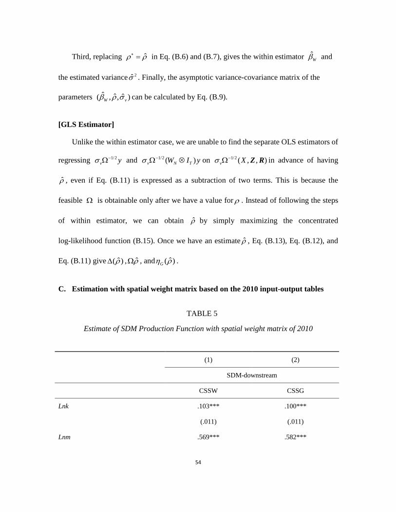
54

Third, replacing ˆρ ρ∗ = in Eq. (B.6) and (B.7), gives the within estimator ˆWβ and

the estimated variance 2σ . Finally, the asymptotic variance-covariance matrix of the

parameters ˆ ˆ ˆ( , , )W vβ ρ σ can be calculated by Eq. (B.9).

[GLS Estimator]

Unlike the within estimator case, we are unable to find the separate OLS estimators of

regressing 1/2v yσ −Ω and 1/2 ( )v N TW I yσ −Ω ⊗ on 1/2 ( , , )v Xσ −Ω Z R in advance of having

ρ , even if Eq. (B.11) is expressed as a subtraction of two terms. This is because the

feasible Ω is obtainable only after we have a value for ρ . Instead of following the steps

of within estimator, we can obtain ρ by simply maximizing the concentrated

log-likelihood function (B.15). Once we have an estimate ρ , Eq. (B.13), Eq. (B.12), and

Eq. (B.11) give ˆ( )ρ∆ , ρΩ , and ˆ( )Gη ρ .

C. Estimation with spatial weight matrix based on the 2010 input-output tables

TABLE 5

Estimate of SDM Production Function with spatial weight matrix of 2010

(1) (2)

SDM-downstream

CSSW CSSG

Lnk .103*** .100***

(.011) (.011)

Lnm .569*** .582***

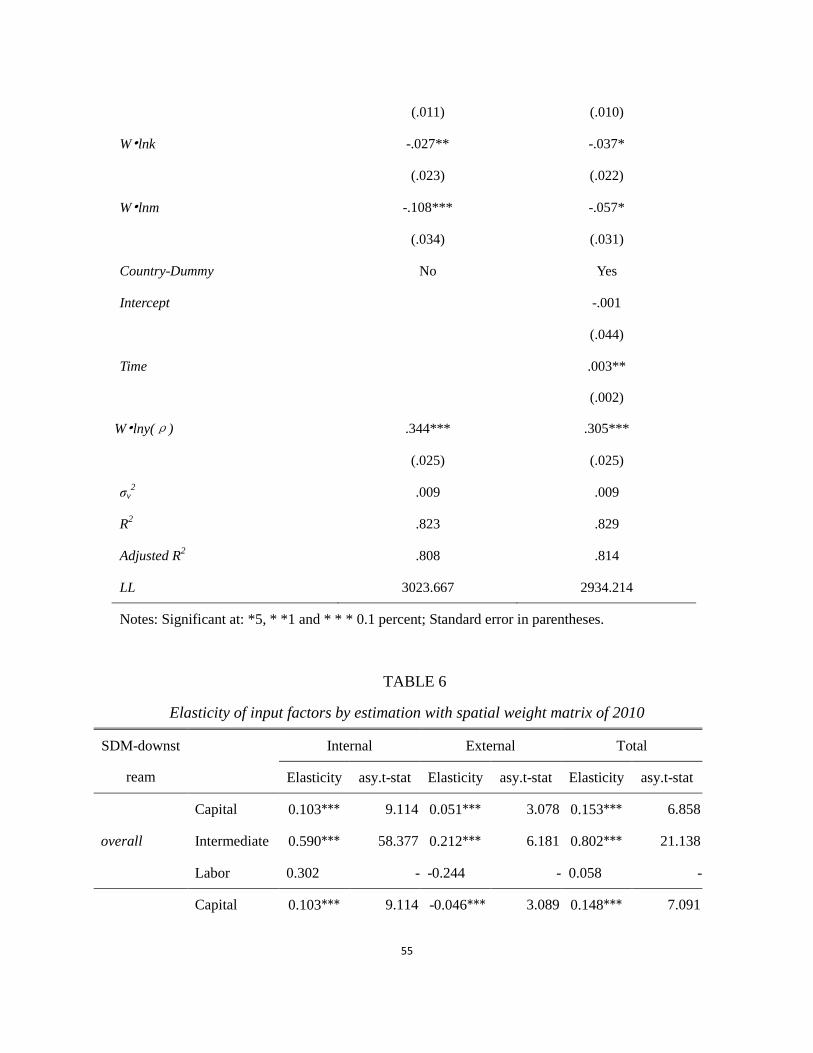
55

(.011) (.010)

W•lnk -.027** -.037*

(.023) (.022)

W•lnm -.108*** -.057*

(.034) (.031)

Country-Dummy No Yes

Intercept -.001

(.044)

Time .003**

(.002)

W•lny(ρ) .344*** .305***

(.025) (.025)

σv2 .009 .009

R2 .823 .829

Adjusted R2 .808 .814

LL 3023.667 2934.214

Notes: Significant at: *5, * *1 and * * * 0.1 percent; Standard error in parentheses.

TABLE 6

Elasticity of input factors by estimation with spatial weight matrix of 2010

SDM-downst

ream

Internal External Total

Elasticity asy.t-stat Elasticity asy.t-stat Elasticity asy.t-stat

Capital 0.103*** 9.114 0.051*** 3.078 0.153*** 6.858

overall Intermediate 0.590*** 58.377 0.212*** 6.181 0.802*** 21.138

Labor 0.302 - -0.244 - 0.058 -

Capital 0.103*** 9.114 -0.046*** 3.089 0.148*** 7.091

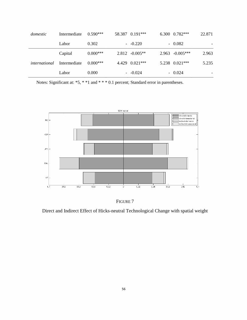
56

domestic Intermediate 0.590*** 58.387 0.191*** 6.300 0.782*** 22.871

Labor 0.302 - -0.220 - 0.082 -

Capital 0.000*** 2.812 -0.005** 2.963 -0.005*** 2.963

international Intermediate 0.000*** 4.429 0.021*** 5.238 0.021*** 5.235

Labor 0.000 - -0.024 - 0.024 -

Notes: Significant at: *5, * *1 and * * * 0.1 percent; Standard error in parentheses.

FIGURE 7

Direct and Indirect Effect of Hicks-neutral Technological Change with spatial weight

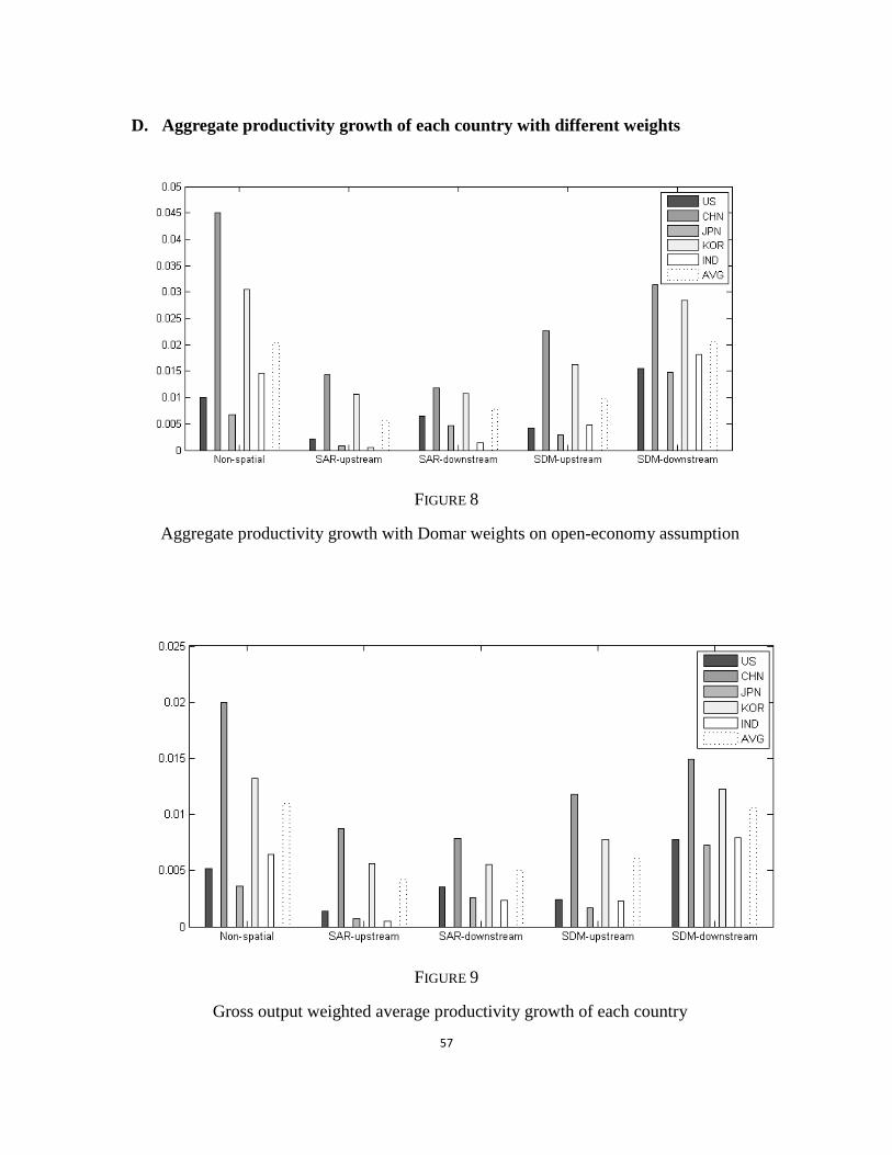
57

D. Aggregate productivity growth of each country with different weights

FIGURE 8

Aggregate productivity growth with Domar weights on open-economy assumption

FIGURE 9

Gross output weighted average productivity growth of each country