Embed Size (px)
Citation preview
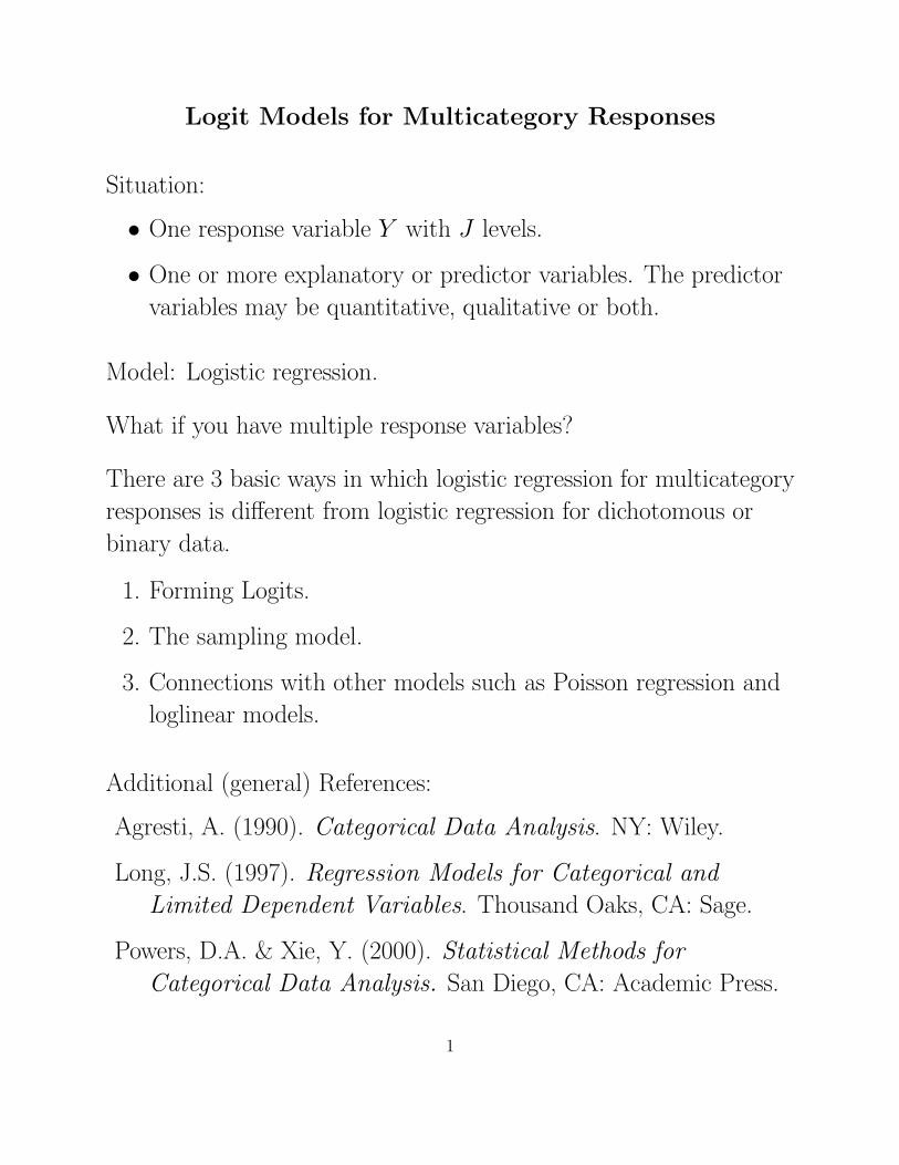
Logit Models for Multicategory Responses
Situation:
• One response variable Y with J levels.
• One or more explanatory or predictor variables. The predictor
variables may be quantitative, qualitative or both.
Model: Logistic regression.
What if you have multiple response variables?
There are 3 basic ways in which logistic regression for multicategory
responses is different from logistic regression for dichotomous or
binary data.
1. Forming Logits.
2. The sampling model.
3. Connections with other models such as Poisson regression and
loglinear models.
Additional (general) References:
Agresti, A. (1990). Categorical Data Analysis. NY: Wiley.
Long, J.S. (1997). Regression Models for Categorical and
Limited Dependent Variables. Thousand Oaks, CA: Sage.
Powers, D.A. & Xie, Y. (2000). Statistical Methods for
Categorical Data Analysis. San Diego, CA: Academic Press.
1

Additional References on Fitting (Conditional) Multinomial Models
using SAS:
SAS Institute (1995). Logistic Regression Examples Using the
SAS System, (version 6). Cary, NC: SAS Institute.
Kuhfeld, W.F. (2001). Marketing Research Methods in the SAS
System, Version 8.2 Edition, TS-650. Cary, NC: SAS Institute.
http://www.sas.com/service/techsup/tnote/tnote stat.html
(reports TS-650A – TS-560I).
Search
http://www.sas.com/service/techsup/tnote/tnote stat.html.
2

Forming Logits
When J = 2, Y is dichotomous and we can model logs of odds
that an event occurs or does not occur. There is only 1 logit
that we can form
logit(π) = log
π
1 − π
When J > 2, . . .
• We have a multicategory or “polytomous” or
“polychotomous” response variable.
• There are J(J − 1)/2 logits (odds) that we can form, but
only (J − 1) are non-redundant.
• There are different ways to form a set of (J − 1)
non-redundant logits.
How to “dichotomized” the response Y ?
1. Nomnial Y —
(a) “Baseline” logit models or “Multinomial” logistic regression.
(b) “Conditional” or “Multinomial” logit models.
2. Ordinal Y —
(a) Cumulative logits.
(b) Adjacent categories.
(c) Continuation ratios.
(These are the most common and generally the most useful ones).
3

Sampling Model.
With dichotomous Y , at each combination of levels of the
explanatory variables, we assume data arise from a Binomial
distribution.
e.g., “Brewed, bottled or powered: Testing the health effects of
tea.” (Nov, 1999). Consumer Reports, pp. 60–61.
Results of clinical study by Junshi Chen of Chinese Academy.
Pre-cancerous Mouth
Lesions
Worse or Shrink
no change (improve)
green tea 18 11 29
placebo 27 3 30
59
With J > 2, at each combination of levels of the explanatory
variables, we assume a Multinomial distribution.
e.g.,
Pre-cancerous Mouth
Lesions
Worse No change Shrink
green tea 29
placebo 30
4

Connections with other Models.
1. Some are equivalent to Poisson regression or loglinear models.
2. Some can be derived from (equivalent to) discrete choice
models (e.g., Luce, McFadden).
3. Those that are equivalent to conditional multinomial models
are equivalent to proportional hazard models (models for
survival data), which is equivalent to Poisson regression model.
4. Some can be derived from latent variable models.
5. Some multicategory logit models are very similar to IRT
models in terms of their parametric form. The difference
between them is that in the IRT models, the predictor is
unobserved (latent), and in the model we discuss here, the
predictor variable is observed.
6. Others.
5

Nominal Response
Y has J categories (order is irrelevant).
{π1, π2, . . . , πJ} are probabilities that response is in each category.
π1 + π2 + . . . + πJ =∑J
j=1 πj = 1.
The probability distribution for the number of outcomes that occur
in the J categories for a sample of n independent observations is
Multinomial.
• The Binomial distribution is a special case of the Multinomial.
• The multinomial distribution depends on n & {π1, π2, . . . , πJ}.
• The multinomial distribution gives the probability for each way
to classify the n observations into the J categories of the
response variable.
For example, the possible ways to classify n = 2 observations
into J = 3 categories is
y1 y2 y3
2 0 0
1 1 0
1 0 1
0 2 0
0 1 1
0 0 2
6
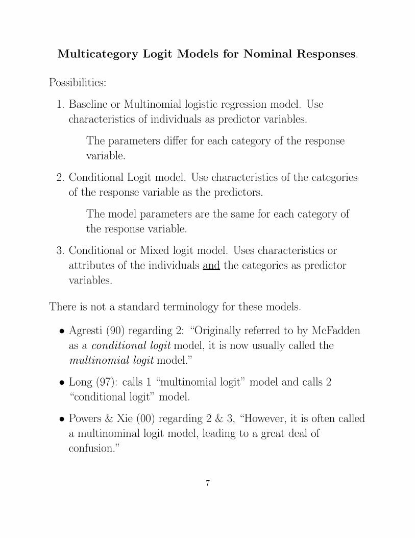
Multicategory Logit Models for Nominal Responses.
Possibilities:
1. Baseline or Multinomial logistic regression model. Use
characteristics of individuals as predictor variables.
The parameters differ for each category of the response
variable.
2. Conditional Logit model. Use characteristics of the categories
of the response variable as the predictors.
The model parameters are the same for each category of
the response variable.
3. Conditional or Mixed logit model. Uses characteristics or
attributes of the individuals and the categories as predictor
variables.
There is not a standard terminology for these models.
• Agresti (90) regarding 2: “Originally referred to by McFadden
as a conditional logit model, it is now usually called the
multinomial logit model.”
• Long (97): calls 1 “multinomial logit” model and calls 2
“conditional logit” model.
• Powers & Xie (00) regarding 2 & 3, “However, it is often called
a multinominal logit model, leading to a great deal of
confusion.”
7

Baseline/Multinomial Category Logit Model
The models we consider here give a simultaneous representation
(summary, description) of the odds of being in one category relative
to being in another category for all pairs of categories.
We need a set of (J − 1) non-redundant odds (logits). Given this,
we can figure out the odds for any pair of categories.
This model is basically just an extension of the binary logistic
regression model.
Consider the HSB data:
Response variable is High school program (HSP) type where
1. General
2. Academic
3. Vo/Tech
Explanatory variables maybe
• Mean of the five achievement test scores, which is
numerical/continuous (xi).
• Socio-economic status, which will be either nominal (βsi ) or
ordinal/numerical (si).
• School type, which would be nominal (public, private).
8

We could fit a binary logit model to each pair of program types:
log
general
academic
= log
π1(xi)
π2(xi)
= α1 + β1xi
log
academic
vo/tech
= log
π2(xi)
π3(xi)
= α2 + β2xi
log
general
vo/tech
= log
π1(xi)
π3(xi)
= α3 + β3xi
We can write one of the odds in terms of the other 2,π1(xi)
π2(xi)
π2(xi)
π3(xi)
=
π1(xi)
π3(xi),
Therefore,we can find the model parameters of one from the other 2,
log
π1(xi)
π2(xi)
+ log
π2(xi)
π3(xi)
= log
π1(xi)
π3(xi)
(α1 + β1xi) + (α2 + β2xi) = α3 + β3xi
which means that in the Population
α1 + α2 = α3
β1 + β2 = β3
9
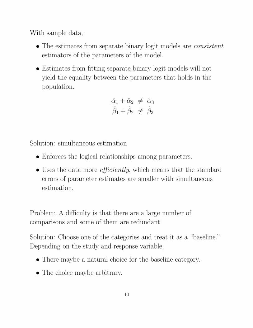
With sample data,
• The estimates from separate binary logit models are consistent
estimators of the parameters of the model.
• Estimates from fitting separate binary logit models will not
yield the equality between the parameters that holds in the
population.
α̂1 + α̂2 �= α̂3
β̂1 + β̂2 �= β̂3
Solution: simultaneous estimation
• Enforces the logical relationships among parameters.
• Uses the data more efficiently, which means that the standard
errors of parameter estimates are smaller with simultaneous
estimation.
Problem: A difficulty is that there are a large number of
comparisons and some of them are redundant.
Solution: Choose one of the categories and treat it as a “baseline.”
Depending on the study and response variable,
• There maybe a natural choice for the baseline category.
• The choice maybe arbitrary.
10

Baseline Category Logit Model
For convenience, we’ll use the last level of the response variable as
the baseline (i.e., the Jth level or category ).
log
πij
πiJ
for j = 1, . . . , J − 1
The baseline category logit model with one explanatory variable x is
log
πij
πiJ
= αj + βjxi for j = 1, . . . , J − 1
• For J = 2, this is just regular (binary) logistic regression.
logit(π) = α + βx
• For J > 2, α and β can differ depending on which 2 categories
are being compared.
• The odds for any pair of categories of Y that can be formed are
a function of the parameters of the model.
Example: the HSB data where
Response variable is High school program (HSP) type where
1. General
2. Academic
3. Vo/Tech
Explanatory variable is the mean of the five achievement test
scores, which is numerical/continuous (xi).
11

For this example, we have (3 − 1) = 2 non-redundant logits (odds):
log
general
vo/tech
= log
π1
π3
= α1 + β1x
log
academic
vo/tech
= log
π2
π3
= α2 + β2x
The logit for (1) general and (2) academic equals
log
π1
π2
= log
π1/π3
π2/π3
= log(π1/π3) − log(π2/π3)
= (α1 + β1x) − (α2 + β2x)
= (α1 − α2) + (β1 − β2)x
The differences (β1 − β2) are known as “contrasts”.
Caution: You must be certain what the computer program that
you use to estimate the model is doing.
• Programs that explicitly estimate the “baseline” logit model
generally either set β1 = 0 or set βJ = 0, and some set the sum∑
j βj = 0.
• Programs that fit the “multinomial” logit model may set
β1 = 0, βJ = 0, or∑
j βj = 0.
12

Again. . . the estimation should be simultaneous, because
• Simultaneous fitting is more efficient.
• The standard errors of parameter estimates are smaller when
model is fit all at once.
• Want to impose the logical relationships among the parameters.
In SAS, this model can be estimated using either
• CATMOD
• GENMOD
Example: estimated model for High School and Beyond
general/votech: ˆlog(π1/π3) = −2.8996 + .0599x
academic/votech: ˆlog(π2/π3) = −7.9388 + .1699x
and for comparing general and academic
ˆlog(π1/π2) = ˆlog(π1/π3) − ˆlog(π2/π3)
= −2.8996 + .0599x − (−7.9388 + .1699x)
= 5.039 − .110x
If we use either general or academic instead of votech as the
baseline category, we get the exact same results.
13

The results using votech as the baseline were obtained using
SAS/CATMOD:
data hsb;
set sasdata.hsb;
achieve=(RDG+WRTG+MATH+SCI+CIV)/5;
proc catmod;
response logits;
direct achieve;
model hsp = achieve ;
title ’Baseline/multinomial logit model: achieve’;
Edited output from CATMOD:
The CATMOD Procedure
Data Summary
Response HSP Response Levels 3
Weight Variable None Populations 490
Data Set HSB Total Frequency 600
Frequency Missing 0 Observations 600
14
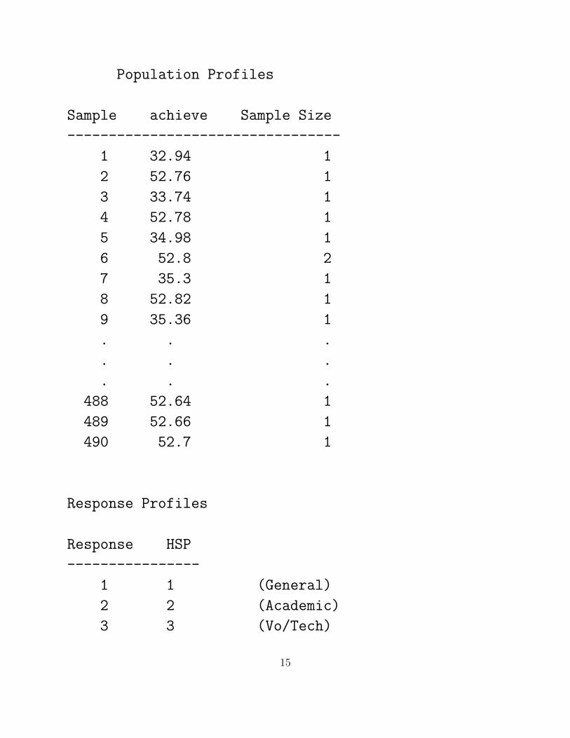
Population Profiles
Sample achieve Sample Size
---------------------------------
1 32.94 1
2 52.76 1
3 33.74 1
4 52.78 1
5 34.98 1
6 52.8 2
7 35.3 1
8 52.82 1
9 35.36 1
. . .
. . .
. . .
488 52.64 1
489 52.66 1
490 52.7 1
Response Profiles
Response HSP
----------------
1 1 (General)
2 2 (Academic)
3 3 (Vo/Tech)
15

Maximum Likelihood Analysis
Sub -2 Log Convergence
Iteration Iteration Likelihood Criterion
----------------------------------------------------
0 0 1318.3347 1.0000
1 0 1087.9513 0.1748
2 0 1083.8083 0.003808
3 0 1083.7834 0.0000230
4 0 1083.7834 1.2814E-9
Parameter Estimates
Iteration 1 2 3 4
--------------------------------------------------------
0 0 0 0 0
1 -1.8247 -6.7704 0.0349 0.1457
2 -2.8551 -7.8374 0.0590 0.1677
3 -2.8992 -7.9380 0.0599 0.1698
4 -2.8996 -7.9388 0.0599 0.1699
Maximum likelihood computations converged.
16
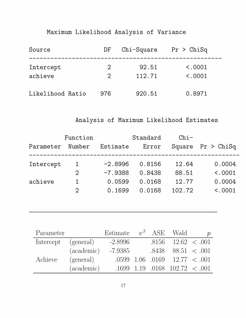
Maximum Likelihood Analysis of Variance
Source DF Chi-Square Pr > ChiSq
------------------------------------------------------
Intercept 2 92.51 <.0001
achieve 2 112.71 <.0001
Likelihood Ratio 976 920.51 0.8971
Analysis of Maximum Likelihood Estimates
Function Standard Chi-
Parameter Number Estimate Error Square Pr > ChiSq
-----------------------------------------------------------
Intercept 1 -2.8996 0.8156 12.64 0.0004
2 -7.9388 0.8438 88.51 <.0001
achieve 1 0.0599 0.0168 12.77 0.0004
2 0.1699 0.0168 102.72 <.0001
Parameter Estimate eβ ASE Wald p
Intercept (general) -2.8996 .8156 12.62 < .001
(academic) -7.9385 .8438 88.51 < .001
Achieve (general) .0599 1.06 .0169 12.77 < .001
(academic) .1699 1.19 .0168 102.72 < .001
17
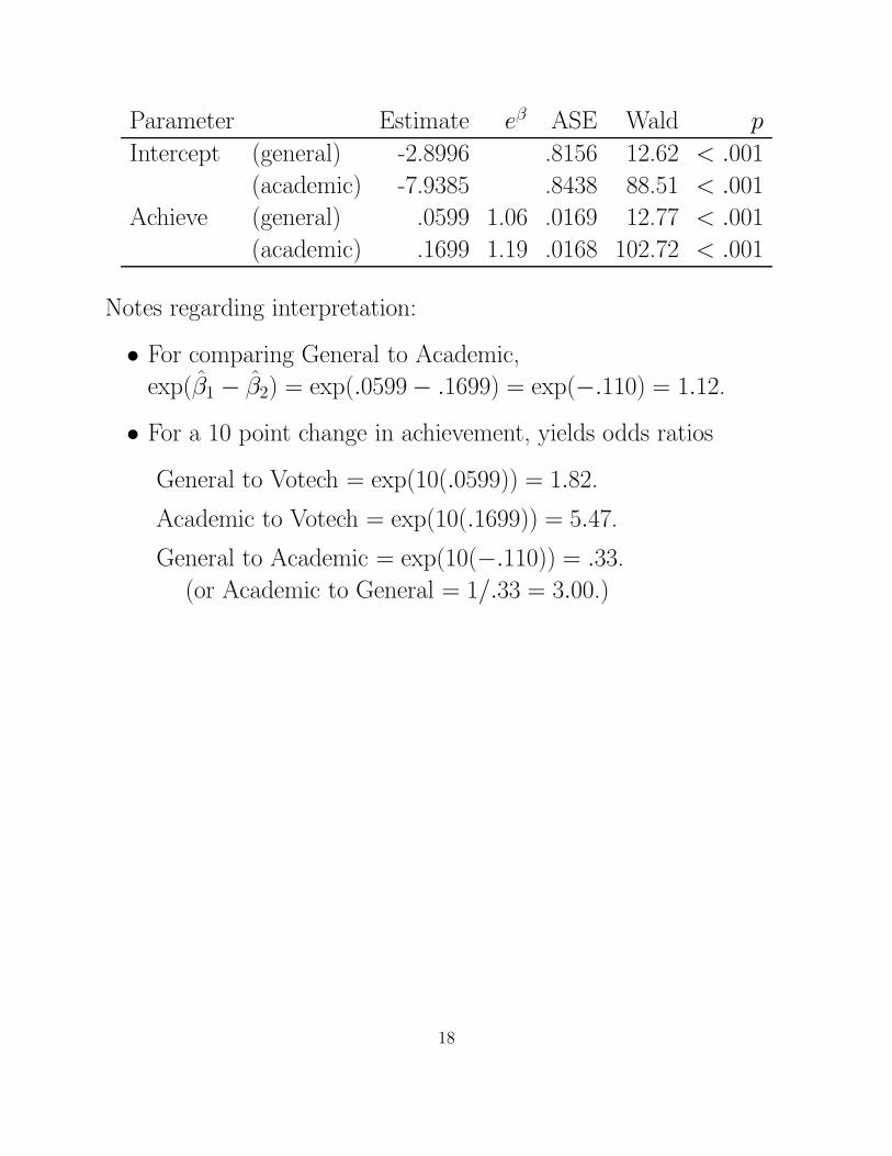
Parameter Estimate eβ ASE Wald p
Intercept (general) -2.8996 .8156 12.62 < .001
(academic) -7.9385 .8438 88.51 < .001
Achieve (general) .0599 1.06 .0169 12.77 < .001
(academic) .1699 1.19 .0168 102.72 < .001
Notes regarding interpretation:
• For comparing General to Academic,
exp(β̂1 − β̂2) = exp(.0599 − .1699) = exp(−.110) = 1.12.
• For a 10 point change in achievement, yields odds ratios
General to Votech = exp(10(.0599)) = 1.82.
Academic to Votech = exp(10(.1699)) = 5.47.
General to Academic = exp(10(−.110)) = .33.
(or Academic to General = 1/.33 = 3.00.)
18
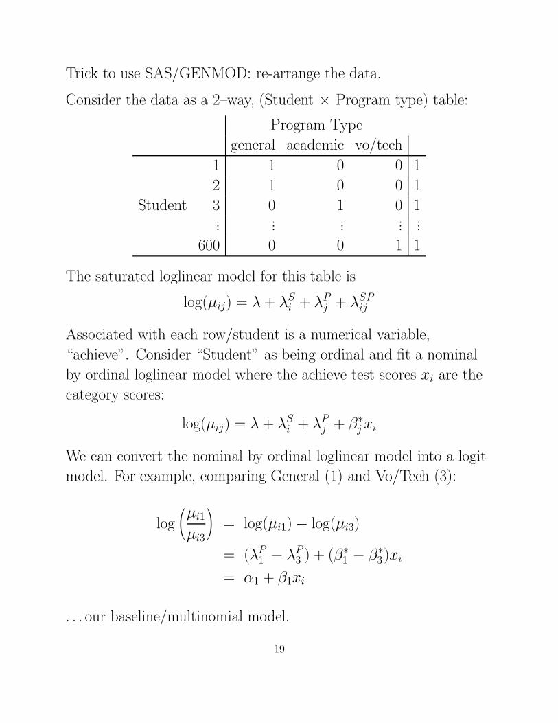
Trick to use SAS/GENMOD: re-arrange the data.
Consider the data as a 2–way, (Student × Program type) table:
Program Type
general academic vo/tech
1 1 0 0 1
2 1 0 0 1
Student 3 0 1 0 1... ... ... ... ...
600 0 0 1 1
The saturated loglinear model for this table is
log(µij) = λ + λSi + λP
j + λSPij
Associated with each row/student is a numerical variable,
“achieve”. Consider “Student” as being ordinal and fit a nominal
by ordinal loglinear model where the achieve test scores xi are the
category scores:
log(µij) = λ + λSi + λP
j + β∗j xi
We can convert the nominal by ordinal loglinear model into a logit
model. For example, comparing General (1) and Vo/Tech (3):
log
µi1
µi3
= log(µi1) − log(µi3)
= (λP1 − λP
3 ) + (β∗1 − β∗
3)xi
= α1 + β1xi
. . . our baseline/multinomial model.
19

Using SAS/GENMOD. . .
data hsp2;
input student hsp count achieve;
datalines;1 1 1 41.32
1 2 0 41.32
1 3 0 41.32... ... ... ...
600 1 0 43.44
600 2 0 43.44
600 3 1 43.44
proc genmod;
class student hsp;
model count = student hsp hsp*achieve / link=log
dist=Poi;
“Student” ensures that the sum of each row of the fitted values
equals 1 (fixed by design) — the λSi ’s or “nuisance” parameters.
“HSP” ensures that the program type margin is fit perfectly — the
λPj ’s which gives us the αj’s in the logit model.
“HSP*achieve” — the β∗j which gives the parameter estimates for
the βj’s in the logit model.
20

Given that SAS/GENMOD sets λP3 = 0 and β∗
3 = 0, you get the
correct ASE errors for the αj’s and βj’s:
Since
αj = (λPj − λP
3 ) = λPj
The ASE of αj simply equals the ASE of λPj .
Since
βj = (β∗j − β∗
3) = β∗j
The ASE of βj simply equals ASE of β∗j
Using either CATMOD or GENMOD, you can easily add more
explanatory variables. For example,
GENMOD:
• SES as a nominal variable:
proc genmod;
class student hsp ses;
model count = student hsp hsp*achieve hsp*ses
/ link=log dist=Poi;
• SES as a numerical variable (e.g., SES=1,2,3)
proc genmod;
class student hsp;
model count = student hsp hsp*achieve hsp*ses
/ link=log dist=Poi;
21

CATMOD:
• SAS as a nominal variable:
proc catmod;
response logits;
direct achieve;
model hsp = achieve ses ;
title ’Achieve numerical and SES qualitative’;
• SAS as a numerical (ordinal) variable:
proc catmod;
response logits;
direct achieve ses ;
model hsp = achieve ses;
title ’Both achieve and ses as numerical variable’;
Other programs that I’ve used to fit multinomial models.
• Vermunt, J.K. (1997). �EM: A General Program for the
Analysis of Categorical Data. Tilburg, University.
www.kub.nl/fsw/organisatie/departmenten/mto/software2.html.
• FORTRAN program that I wrote.
Other programs that I know of (but haven’t used).
• SYSTAT
• SPSS
22

To illustrate the need for simultaneous estimation . . . the binary
logistic regression model was fit separately to 2 of the 3 possible
logits,
log
π1
π3
= α1 + β1x
log
π2
π3
= α2 + β2x
yields
Simultaneous Fit Separate Fit
Parameter Estimate ASE Esiatmate ASE
Intercept (general) -2.8996 .8156 -2.9656 .8342
(academic) -7.9385 .8438 -7.5311 .8572
Achieve (general) .0599 .0169 .0613 .0172
(academic) .1699 .0168 .1618 .0170
23
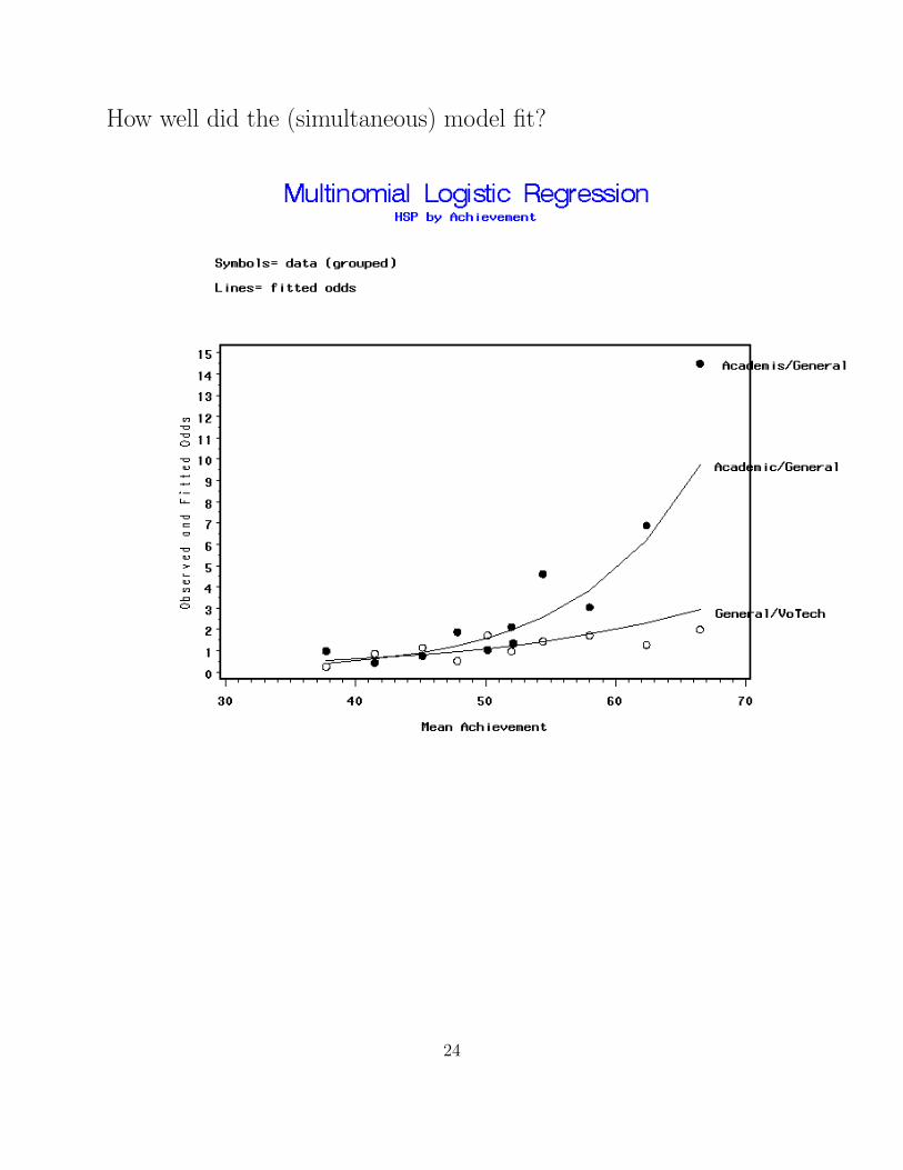
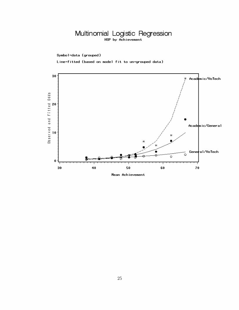
How well did the (simultaneous) model fit?
24
25

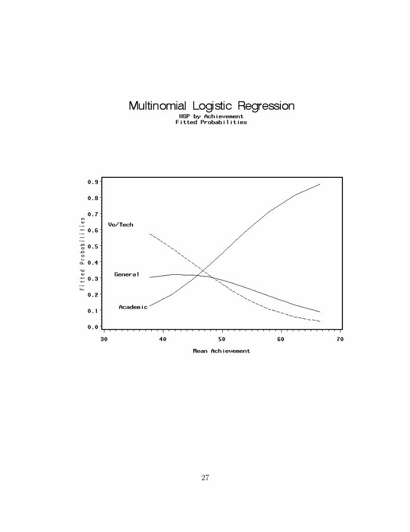
Computing Probabilities from the
Baseline Logit Model.
Just as in logistic regression for J = 2, we can talk about (and
interpret) baseline category logit model in terms of probabilities.
The probability of a response being in category j is
πj =exp(αj + βjx)
∑Jh=1 exp(αh + βhx)
Note:
• The denominator∑J
h=1 exp(αh + βhx) ensures that∑J
j=1 πj = 1.
• αJ = 0 and βJ = 0 (baseline), which is an identification
constraint.
Example: High school and beyond
π̂votech =1
1 + exp(−2.90 + .06x) + exp(−7.94 + .17x)
π̂general =exp(−2.90 + .06x)
1 + exp(−2.90 + .06x) + exp(−7.94 + .17x)
π̂academic =exp(−7.94 + .17x)
1 + exp(−2.90 + .06x) + exp(−7.94 + .17x)
which when plotted versus mean achievement scores. . .
26
27

Statistical Inference
There are 2 kinds of tests we’ll talk about here:
1. Test whether an explanatory variable is related to the response
variable.
2. Test whether the parameters for two (or more) categories of the
response variable are the same.
Both of these tests can be done using either Wald or likelihood
ratio (LR) tests. We’ll talk about LR tests here; see Long (1997) for
the Wald tests.
Test whether an explanatory/predictor variable is not related to the
response; that is,
Ho : βk1 = . . . = βkJ = 0
for the kth explanatory variable.
Example of LR test: Consider HSB example but now include SES
as a nominal variable and then as an ordinal variable.
From the CATMOD output,
Model −2Log(like) ∆df ∆G2 p-value
achieve, nominal SES 1064.6659 — — —
achieve, ordinal SES 1068.2397 2 3.57 .16
achieve 1083.7834 2 15.54 < .001
28
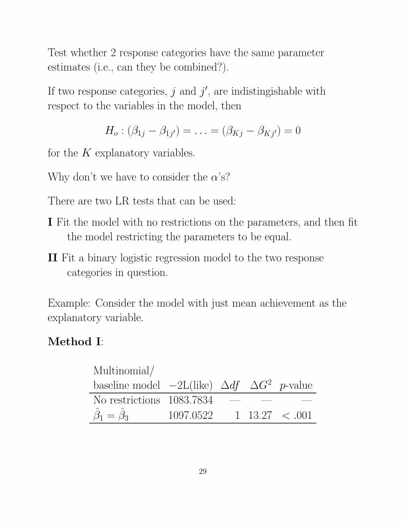
Test whether 2 response categories have the same parameter
estimates (i.e., can they be combined?).
If two response categories, j and j′, are indistingishable with
respect to the variables in the model, then
Ho : (β1j − β1j′) = . . . = (βKj − βKj′) = 0
for the K explanatory variables.
Why don’t we have to consider the α’s?
There are two LR tests that can be used:
I Fit the model with no restrictions on the parameters, and then fit
the model restricting the parameters to be equal.
II Fit a binary logistic regression model to the two response
categories in question.
Example: Consider the model with just mean achievement as the
explanatory variable.
Method I:
Multinomial/
baseline model −2L(like) ∆df ∆G2 p-value
No restrictions 1083.7834 — — —
β̂1 = β̂3 1097.0522 1 13.27 < .001
29

Notes regarding Method I:
• This can be done easily using GENMOD.
• The trick is to create a new variable that is used to impose the
equality restriction.
data hsblong;
input student hsp count achieve;
* Create a new dummy variable for equating
parameters for votech (hsp=3) and general (hsp=1);
xhsp=0;
if hsp=2 then xhsp=1;
datalines;
1 1 1 41.32000
1 2 0 41.32000
1 3 0 41.32000
2 1 1 45.02000
2 2 0 45.02000
2 3 0 45.02000
3 1 1 34.98000
...
600 1 0 43.44000
600 2 0 43.44000
600 3 1 43.44000
30

proc genmod;
class student hsp;
model count = student hsp hsp*achieve
/ link=log dist=poi;
title ’Full Model (no restrictions)’;
proc genmod;
class student hsp;
model count = student hsp xhsp*achieve
/ link=log dist=poi;
title ’Equate the slope parameters for
votech and general’;
• You can use this method to check whether a sub-set of or
specific parameters are equal.
• You can use this trick to see if the parameters for more than
two response categories are the same.
31

Method II: Using the binary logistic regression model to test
Ho : (β1j − β2j′) = . . . = (βKj − βKj′) = 0
for the K explanatory variables.
1. Create a new dataset that only contains the observations from
response categories j and j′.
2. Fit the binary logistic regression model to the new dataset.
3. Compute the likelihood ratio statistic that all the slope
coefficients (βk’s) are simultaneously equal to 0 — not the
intercept term..
Example: We have
LR=13.49 with df = 1, p < .001.
Notes regarding Methods I and II:
• In this case, both methods give similar results (Method I:
LR= 13.27).
• Method I is more flexible in terms of the range of possible tests
that can be performed.
• The Method II is much easier. Just how easy this is,
32

Input
data hsb;
set sasdata.hsb;
achieve=(RDG+WRTG+MATH+SCI+CIV)/5;
if hsp=2 then delete;
proc logistic descending;
model hsp = achieve;
Edited Output:
The LOGISTIC Procedure
Model Information
Data Set WORK.HSB
Response Variable HSP
Number of Response Levels 2
Number of Observations 292
Model binary logit
Optimization Technique Fisher’s scoring
33

Response Profile
Ordered Total
Value HSP Frequency
1 3 147
2 1 145
Probability modeled is HSP=3.
Model Convergence Status
Convergence criterion (GCONV=1E-8) satisfied.
Model Fit Statistics
Intercept
Intercept and
Criterion Only Covariates
AIC 406.784 395.293
SC 410.461 402.647
-2 Log L 404.784 391.293
Testing Global Null Hypothesis: BETA=0
Test Chi-Square DF Pr > ChiSq
Likelihood Ratio 13.4910 1 0.0002
Score 13.2434 1 0.0003
Wald 12.7559 1 0.0004
34

Baseline/Multinomial Logit model
and Grouped Data
(Loglinear Model Connection)
When the explanatory/predictor variables are all categorical, the
baseline category logit model has an equivalent loglinear model.
Example: Data from Fienberg (1985). In 1963, 2400 men who were
rejected for military service because they failed the Armed Forces
Qualitifcation Test were interviewed. The data from 2294 of them
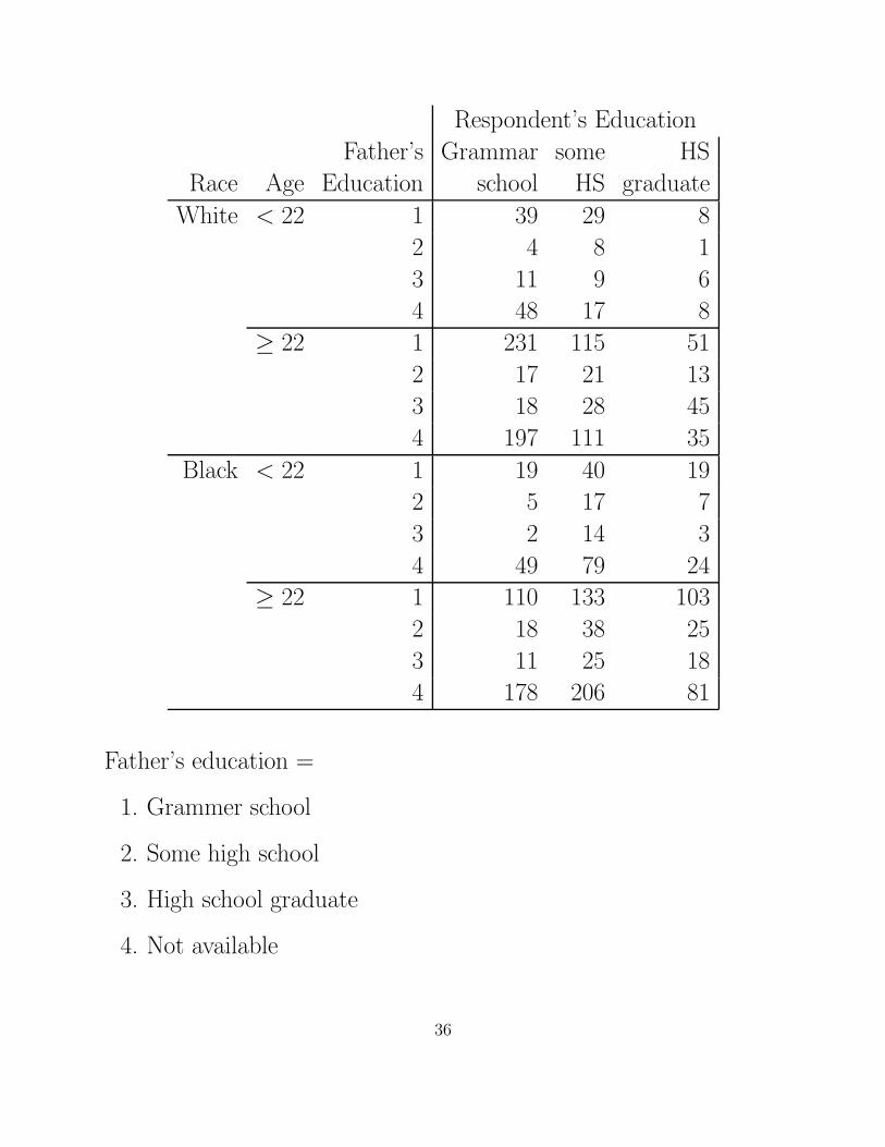
were as 4–way cross-classification is given below.
The response variable is E (respondenent’s education) =
grammar school, some HS, HS graduate.
The 3 explanatory variables are
R (Race) = White, Black.
A (age) = under 22, 22 or older.
F (father’s education) = 1 (grammar school), 2 (some HS),
3 (HS graduate), 4 (not available).
35
Respondent’s Education
Father’s Grammar some HS
Race Age Education school HS graduate
White < 22 1 39 29 8
2 4 8 1
3 11 9 6
4 48 17 8
≥ 22 1 231 115 51
2 17 21 13
3 18 28 45
4 197 111 35
Black < 22 1 19 40 19
2 5 17 7
3 2 14 3
4 49 79 24
≥ 22 1 110 133 103
2 18 38 25
3 11 25 18
4 178 206 81
Father’s education =
1. Grammer school
2. Some high school
3. High school graduate
4. Not available
36
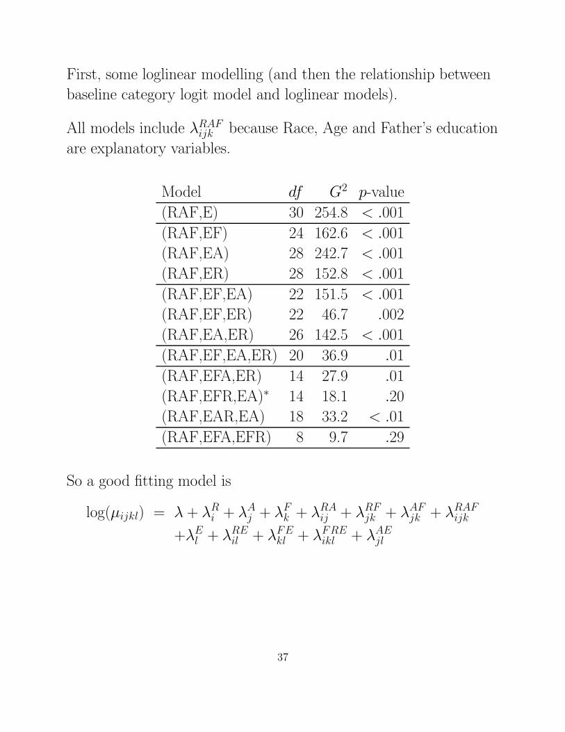
First, some loglinear modelling (and then the relationship between
baseline category logit model and loglinear models).
All models include λRAFijk because Race, Age and Father’s education
are explanatory variables.
Model df G2 p-value
(RAF,E) 30 254.8 < .001
(RAF,EF) 24 162.6 < .001
(RAF,EA) 28 242.7 < .001
(RAF,ER) 28 152.8 < .001
(RAF,EF,EA) 22 151.5 < .001
(RAF,EF,ER) 22 46.7 .002
(RAF,EA,ER) 26 142.5 < .001
(RAF,EF,EA,ER) 20 36.9 .01
(RAF,EFA,ER) 14 27.9 .01
(RAF,EFR,EA)∗ 14 18.1 .20
(RAF,EAR,EA) 18 33.2 < .01
(RAF,EFA,EFR) 8 9.7 .29
So a good fitting model is
log(µijkl) = λ + λRi + λA
j + λFk + λRA
ij + λRFjk + λAF
jk + λRAFijk
+λEl + λRE
il + λFEkl + λFRE
ikl + λAEjl
37
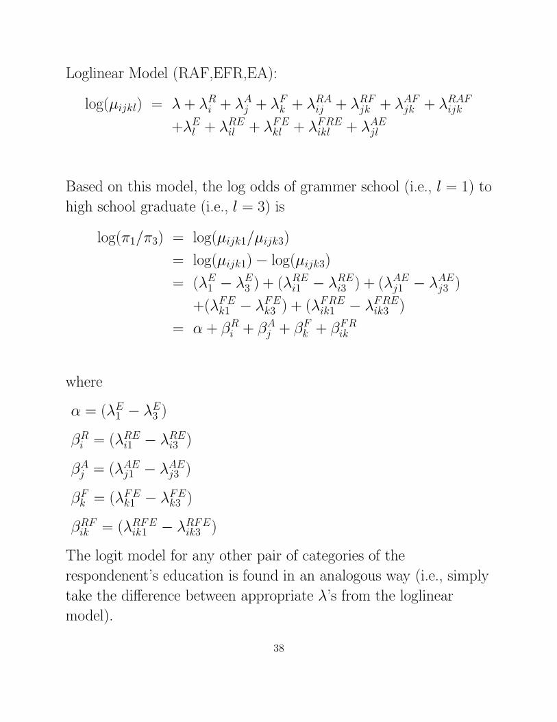
Loglinear Model (RAF,EFR,EA):
log(µijkl) = λ + λRi + λA
j + λFk + λRA
ij + λRFjk + λAF
jk + λRAFijk
+λEl + λRE
il + λFEkl + λFRE
ikl + λAEjl
Based on this model, the log odds of grammer school (i.e., l = 1) to
high school graduate (i.e., l = 3) is
log(π1/π3) = log(µijk1/µijk3)
= log(µijk1) − log(µijk3)
= (λE1 − λE
3 ) + (λREi1 − λRE
i3 ) + (λAEj1 − λAE
j3 )
+(λFEk1 − λFE
k3 ) + (λFREik1 − λFRE
ik3 )
= α + βRi + βA
j + βFk + βFR
ik
where
α = (λE1 − λE
3 )
βRi = (λRE
i1 − λREi3 )
βAj = (λAE
j1 − λAEj3 )
βFk = (λFE
k1 − λFEk3 )
βRFik = (λRFE
ik1 − λRFEik3 )
The logit model for any other pair of categories of the
respondenent’s education is found in an analogous way (i.e., simply
take the difference between appropriate λ’s from the loglinear
model).
38
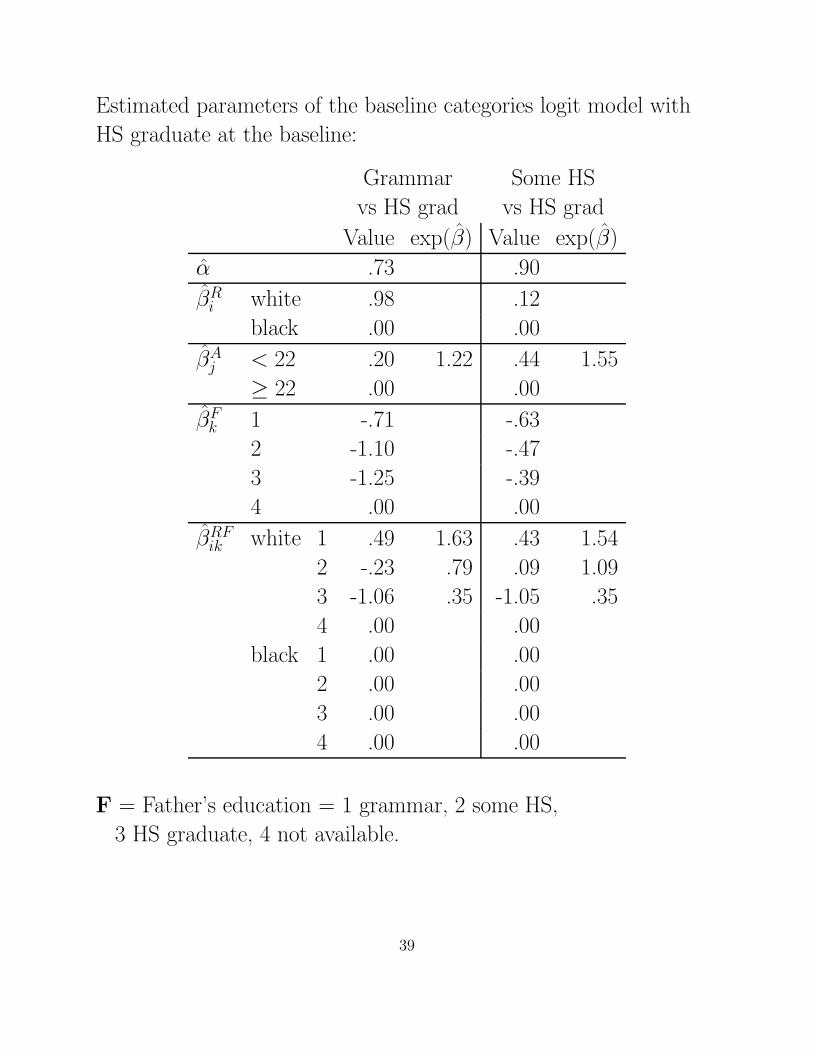
Estimated parameters of the baseline categories logit model with
HS graduate at the baseline:
Grammar Some HS
vs HS grad vs HS grad
Value exp(β̂) Value exp(β̂)
α̂ .73 .90
β̂Ri white .98 .12
black .00 .00
β̂Aj < 22 .20 1.22 .44 1.55
≥ 22 .00 .00
β̂Fk 1 -.71 -.63
2 -1.10 -.47
3 -1.25 -.39
4 .00 .00
β̂RFik white 1 .49 1.63 .43 1.54
2 -.23 .79 .09 1.09
3 -1.06 .35 -1.05 .35
4 .00 .00
black 1 .00 .00
2 .00 .00
3 .00 .00
4 .00 .00
F = Father’s education = 1 grammar, 2 some HS,
3 HS graduate, 4 not available.
39

Some Intpretation:
• Age: The odds that someone younger than 22 has had some
high school (versus graduating) are 1.55 times larger than the
odds for a person older than 22. An older person has had more
time to complete HS.
• 1/.35 = 2.86 =⇒ Given that the father graduated from high
school, the odds that a black completes some high school
(versus graduates) are 2.86 times time larger than the odds
that a white completes some high school (versus graduates).
40
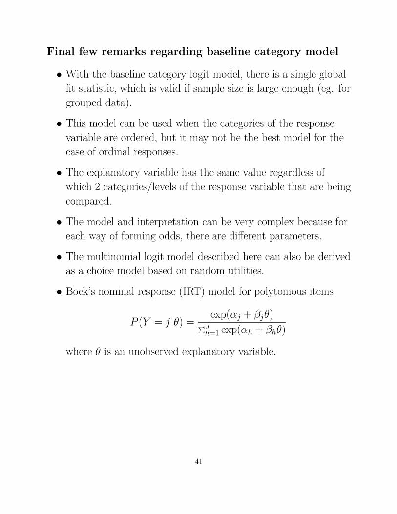
Final few remarks regarding baseline category model
• With the baseline category logit model, there is a single global
fit statistic, which is valid if sample size is large enough (eg. for
grouped data).
• This model can be used when the categories of the response
variable are ordered, but it may not be the best model for the
case of ordinal responses.
• The explanatory variable has the same value regardless of
which 2 categories/levels of the response variable that are being
compared.
• The model and interpretation can be very complex because for
each way of forming odds, there are different parameters.
• The multinomial logit model described here can also be derived
as a choice model based on random utilities.
• Bock’s nominal response (IRT) model for polytomous items
P (Y = j|θ) =exp(αj + βjθ)
∑Jh=1 exp(αh + βhθ)
where θ is an unobserved explanatory variable.
41
Conditional Logit Model
In Psychology, this is either Bradley & Terry (1952) or the Luce
(1959) choice model. In business/economics, this is McFadden’s
(1974) conditional logit model.
Situation: Individuals are given a set of possible choices, which
differ on certain attributes. We would like to model/predict the
probability of choices using the attributes of the choices as
explanatory/predictor variables.
Examples:
• Subjects are given 8 chocolate candies and asked which one
they like the best (SAS Logistic Regression examples, 1995;
Kuhfeld; 2001). The explanatory variables are
– Type of chocolate: milk or dark
– Texture: hard or soft
– Include nuts: nuts or no nuts
• Inidividuals must choose which of 5 brands of a product that
they prefer (SAS Logistic Regression examples, 1995; Kuhfeld;
2001). The explanatory variable is the price of the product.
The company presents different combinations of prices for the
different brands to see how much of an effect this has on choice
behavior.
• The classic example: choice of mode of transportation (eg,
train, bus, car). Characteristics or attributes of these include
time waiting, how long it takes to get to work, and cost.
42

The conditional logit model:
• The coefficients of the explanatory variables are the same over
the categories (choices) of the response variable.
• The values of the explanatory variables differ over the outcomes
(and possibly over individuals).
πj(xij) =exp[α + βxij]
∑jεCi
exp[α + βxij]
where
xij is the value of the explanatory variable for individual i and
response choice j.
The summation in the denominator is over response
options/choices that individual i is given.
Properties of this model:
• The odds that individual i chooses option j versus k is a
function of the difference between xij and xik:
log
πj(xij)
πk(xik)
= β(xij − xik)
• The odds of choosing j versus k does not depend on any of the
other options in the choice set or the other options’ values on
the attribute variables.
Property of “Independence from Irrelevant Alternatives”.
43

• The multinomial/baseline model can be written in the same
form as the conditional logit model model (see Agresti (90), p
316-317).
• This model can incorporate attributes or characteristics of the
decision maker/individual.
• It can be written as a proportional hazard model.
Examples:
1. Three examples that only include attributes of the response
alternatives.
2. An example that includes both attributes of the response
alternatives and characteristics of the individual (“mixed
model”).
44

Example 1: chocolates
The model that was fit is
πj(cj, tj, nj) =exp[α + β1cj + β2tj + β3nj]
∑8h=1(exp[α + β1ch + β2th + β3nh])
where
• Type of chocolate is dummy coded:
cj =
1 if milk
0 if dark
• Texture is dummy coded:
tj =
1 if hard
0 if soft
• Nuts is dummy coded:
nj =
1 if no nuts
0 if nuts
45

Or in terms of Odds:πj(cj, tj, nj)
πk(ck, tk, nk)= exp[β1(cj − ck)] exp[β2(tj − tk)] exp[β3(nj − nk)]
parameter df value ASE Wald p exp β
α 1 -2.88 1.03 7.78 .01 —
Type of chocolate
milk 1 -1.38 .79 3.07 .08 .25 or (1/.25) = 4.00
dark 0 0.00
Texture
hard 1 2.20 1.05 4.35 .04 9.00
soft 0 0.00
Nuts
no nuts 1 -.85 .69 1.51 .22 .43 or (1/.43) = 2.33
nuts 0 0.00
Use exp β for interpretation.
The predicted probabilities.
Obs drk sft nts phat
1 dark hard nuts 0.50400
2 dark hard no n 0.21600
3 milk hard nuts 0.12600
4 dark soft nuts 0.05600
5 milk hard no n 0.05400
6 dark soft no n 0.02400
7 milk soft nuts 0.01400
8 milk soft no n 0.00600
46

Estimation of the model:
1. SAS Logistic Regression Examples (1995) and Kuhfeld (2001;
http://www.sas.com/service/techsup/tnote/tnote stat.html)
describes how this can be done using proc PHREG
(proportional hazard regression), which is related to Poisson
regression. The “trick” here is to dummy code for “time” so
that the non-selected category is 1 and the choosen is 0.
2. The model can be fit as a Poisson regression model using
GENMOD by appropriately arranging the data.
The Data file:
data chocs;
title ’Chocolate Candy Data’;
input subj choose dark soft nuts @@;
t=2-choose; * Needed when using PROC PHREG;
if dark=1 then drk=’dark’; else drk=’milk’; * Needed for printing out table;
if soft=1 then sft=’soft’; else sft=’hard’; * of predicted probabilities;
if nuts=1 then nts=’nuts’; else nts=’no nuts’;
datalines;
1 0 0 0 0 1 0 0 0 1 1 0 0 1 0 1 0 0 1 1
1 1 1 0 0 1 0 1 0 1 1 0 1 1 0 1 0 1 1 1
2 0 0 0 0 2 0 0 0 1 2 0 0 1 0 2 0 0 1 1
2 0 1 0 0 2 1 1 0 1 2 0 1 1 0 2 0 1 1 1
3 0 0 0 0 3 0 0 0 1 3 0 0 1 0 3 0 0 1 1
3 0 1 0 0 3 0 1 0 1 3 1 1 1 0 3 0 1 1 1
4 0 0 0 0 4 0 0 0 1 4 0 0 1 0 4 0 0 1 1
4 1 1 0 0 4 0 1 0 1 4 0 1 1 0 4 0 1 1 1
5 0 0 0 0 5 1 0 0 1 5 0 0 1 0 5 0 0 1 1
5 0 1 0 0 5 0 1 0 1 5 0 1 1 0 5 0 1 1 1
6 0 0 0 0 6 0 0 0 1 6 0 0 1 0 6 0 0 1 1
6 0 1 0 0 6 1 1 0 1 6 0 1 1 0 6 0 1 1 1
7 0 0 0 0 7 1 0 0 1 7 0 0 1 0 7 0 0 1 1
7 0 1 0 0 7 0 1 0 1 7 0 1 1 0 7 0 1 1 1
8 0 0 0 0 8 0 0 0 1 8 0 0 1 0 8 0 0 1 1
8 0 1 0 0 8 1 1 0 1 8 0 1 1 0 8 0 1 1 1
47

9 0 0 0 0 9 0 0 0 1 9 0 0 1 0 9 0 0 1 1
9 0 1 0 0 9 1 1 0 1 9 0 1 1 0 9 0 1 1 1
10 0 0 0 0 10 0 0 0 1 10 0 0 1 0 10 0 0 1 1
10 0 1 0 0 10 1 1 0 1 10 0 1 1 0 10 0 1 1 1
Using SAS/GENMOD:
proc genmod data=chocs;
class subj dark soft nuts;
model choose = dark soft nuts /link=log dist=poi obstats;
output out=fitted pred=phat;
title ’Conditional logit model using GENMOD’;
data subset;
merge chocs fitted;
if subj>1 then delete;
proc sort;
by descending phat;
proc print;
var drk sft nts phat;
title ’Predicted probabilities for different chocolates’;
48

Output from GENMOD
Model Information
Data Set WORK.CHOCS
Distribution Poisson
Link Function Log
Dependent Variable choose
Observations Used 80
Class Level Information
Class Levels Values
subj 10 1 2 3 4 5 6 7 8 9 10
dark 2 0 1
soft 2 0 1
nuts 2 0 1
Criteria For Assessing Goodness Of Fit
Criterion DF Value Value/DF
Deviance 76 28.7270 0.3780
Scaled Deviance 76 28.7270 0.3780
Pearson Chi-Square 76 66.7195 0.8779
Scaled Pearson X2 76 66.7195 0.8779
Log Likelihood -24.3635
Algorithm converged.
49

Analysis Of Parameter Estimates
Standard Wald 95% Chi-
Parameter DF Estimate Error Confidence Limits Square Pr > ChiSq
Intercept 1 -2.8824 1.0334 -4.9078 -0.8570 7.78 0.0053
dark 0 1 -1.3863 0.7906 -2.9358 0.1632 3.07 0.0795
dark 1 0 0.0000 0.0000 0.0000 0.0000 . .
soft 0 1 2.1972 1.0541 0.1312 4.2632 4.35 0.0371
soft 1 0 0.0000 0.0000 0.0000 0.0000 . .
nuts 0 1 -0.8473 0.6901 -2.1998 0.5052 1.51 0.2195
nuts 1 0 0.0000 0.0000 0.0000 0.0000 . .
Scale 0 1.0000 0.0000 1.0000 1.0000
50

Using PROC PHREG.
But first, what’s a proportional hazard regression?
• It’s typically used for modeling surival data; that is, modeling
the time until death (or other event of interest).
• It’s equivalent to a Poisson regression for the number of deaths
and to a negative expontential for survival times.
• For more details see Agresti (1990).
Using SAS PROC PHREG: input
proc phreg data=chocs outest=betas;
strata subj;
model t*choose(0)=dark soft nuts;
title ’Conditional Logit model fit using PROC PHREG’;
run;
Output:
The PHREG Procedure
Model Information
Data Set WORK.CHOCS
Dependent Variable t
Censoring Variable choose
Censoring Value(s) 0
Ties Handling BRESLOW
51

Summary of the Number of Event and Censored Values
Percent
Stratum subj Total Event Censored Censored
1 1 8 1 7 87.50
2 2 8 1 7 87.50
3 3 8 1 7 87.50
4 4 8 1 7 87.50
5 5 8 1 7 87.50
6 6 8 1 7 87.50
7 7 8 1 7 87.50
8 8 8 1 7 87.50
9 9 8 1 7 87.50
10 10 8 1 7 87.50
-------------------------------------------------------------------
Total 80 10 70 87.50
Convergence Status
Convergence criterion (GCONV=1E-8) satisfied.
Model Fit Statistics
Without With
Criterion Covariates Covariates
-2 LOG L 41.589 28.727
AIC 41.589 34.727
SBC 41.589 35.635
Testing Global Null Hypothesis: BETA=0
Test Chi-Square DF Pr > ChiSq
Likelihood Ratio 12.8618 3 0.0049
Score 11.6000 3 0.0089
Wald 8.9275 3 0.0303
Analysis of Maximum Likelihood Estimates
Parameter Standard Hazard
Variable DF Estimate Error Chi-Square Pr > ChiSq Ratio
dark 1 1.38629 0.79057 3.0749 0.0795 4.000
soft 1 -2.19722 1.05409 4.3450 0.0371 0.111
nuts 1 0.84730 0.69007 1.5076 0.2195 2.333
52

Example 2: Five brands that differ in terms of price where price is
manipulated. For each of the 8 combinations of brand and price
included in the study, 100 individuals made their choice.
In all models that we fit, we assume (i.e., fit a parameter) for brand
preference.
The two models that are fit:
1. The effect of price does not depend on brand.
2. The effect of price depends on the brand (i.e. the strength of
brand loyalty depends on price).
Complex model: G2 = 2782.0879
Simpler model: G2 = 2782.4901
LR statistic for testing whether effect of price depends on brand:
G2 = 2782.4901 − 2782.0879 = .4022, df = 3, p = .94
So let’s look at simpler model. . .
53
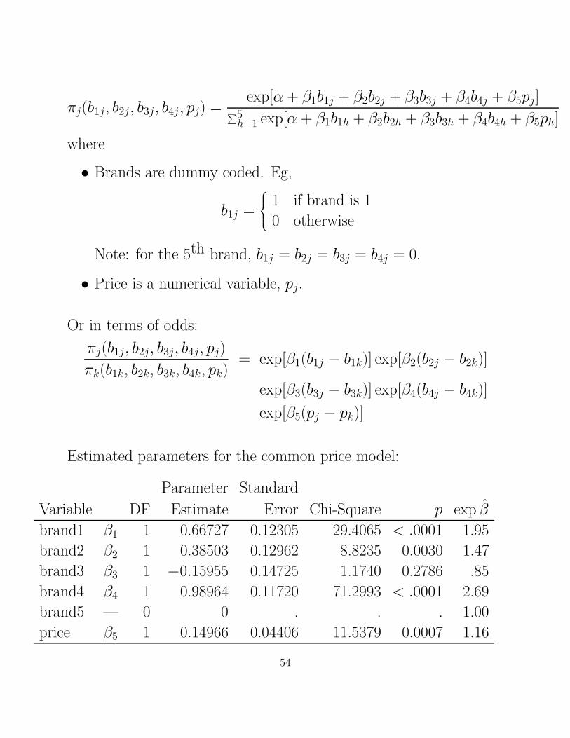
πj(b1j, b2j, b3j, b4j, pj) =exp[α + β1b1j + β2b2j + β3b3j + β4b4j + β5pj]
∑5h=1 exp[α + β1b1h + β2b2h + β3b3h + β4b4h + β5ph]
where
• Brands are dummy coded. Eg,
b1j =
1 if brand is 1
0 otherwise
Note: for the 5th brand, b1j = b2j = b3j = b4j = 0.
• Price is a numerical variable, pj.
Or in terms of odds:
πj(b1j, b2j, b3j, b4j, pj)
πk(b1k, b2k, b3k, b4k, pk)= exp[β1(b1j − b1k)] exp[β2(b2j − b2k)]
exp[β3(b3j − b3k)] exp[β4(b4j − b4k)]
exp[β5(pj − pk)]
Estimated parameters for the common price model:
Parameter Standard
Variable DF Estimate Error Chi-Square p exp β̂
brand1 β1 1 0.66727 0.12305 29.4065 < .0001 1.95
brand2 β2 1 0.38503 0.12962 8.8235 0.0030 1.47
brand3 β3 1 −0.15955 0.14725 1.1740 0.2786 .85
brand4 β4 1 0.98964 0.11720 71.2993 < .0001 2.69
brand5 — 0 0 . . . 1.00
price β5 1 0.14966 0.04406 11.5379 0.0007 1.16
54

• Which brand is the most preferred?
• Which brand is least preferred?
• What is the effect of price?
How would you interpret exp[.1497] = 1.16?
Estimating the common price effect and the price × brand
interaction model using SAS:
GENMOD: as a Poisson regression model.
PHREG: as a proportional harzard model.
First the “raw” data:
data brands;
title ’Brand Choice Data’;
input p1-p5 f1-f5;
datalines;
5.99 5.99 5.99 5.99 4.99 12 19 22 33 14
5.99 5.99 3.99 3.99 4.99 34 26 8 27 5
5.99 3.99 5.99 3.99 4.99 13 37 15 27 8
5.99 3.99 3.99 5.99 4.99 49 1 9 37 4
3.99 5.99 5.99 3.99 4.99 31 12 6 18 33
3.99 5.99 3.99 5.99 4.99 4 29 16 42 9
3.99 3.99 5.99 5.99 4.99 37 10 5 35 13
3.99 3.99 3.99 3.99 4.99 16 14 5 51 14
55

Format of data needed for input to GENMOD:
data brands2;
input combo brand price choice @@;
datalines;
1 1 5.99 12 1 2 5.99 0 1 3 5.99 0 1 4 5.99 0 1 5 4.99 0
1 1 5.99 0 1 2 5.99 19 1 3 5.99 0 1 4 5.99 0 1 5 4.99 0
1 1 5.99 0 1 2 5.99 0 1 3 5.99 22 1 4 5.99 0 1 5 4.99 0
1 1 5.99 0 1 2 5.99 0 1 3 5.99 0 1 4 5.99 33 1 5 4.99 0
1 1 5.99 0 1 2 5.99 0 1 3 5.99 0 1 4 5.99 0 1 5 4.99 14
2 1 5.99 34 2 2 5.99 0 2 3 3.99 0 2 4 3.99 0 2 5 4.99 0
2 1 5.99 0 2 2 5.99 26 2 3 3.99 0 2 4 3.99 0 2 5 4.99 0
2 1 5.99 0 2 2 5.99 0 2 3 3.99 8 2 4 3.99 0 2 5 4.99 0
2 1 5.99 0 2 2 5.99 0 2 3 3.99 0 2 4 3.99 27 2 5 4.99 0
2 1 5.99 0 2 2 5.99 0 2 3 3.99 0 2 4 3.99 0 2 5 4.99 5
etc.
PROC GENMOD commands:
proc genmod;
class combo brand ;
model choice = combo brand price /link=log dist=poi;
title ’Brands Model 1 ’;
proc genmod;
class combo brand ;
model choice = combo brand brand*price /link=log dist=poi;
title ’Brands Model 2 ’;
run;
56
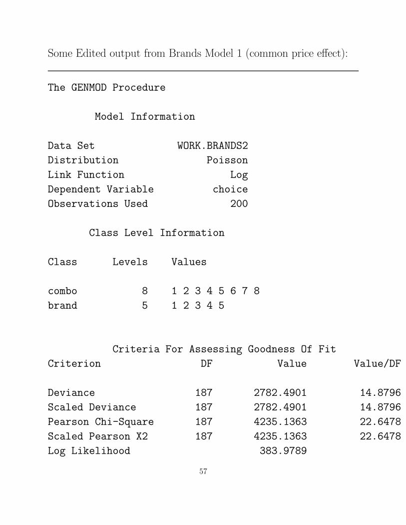
Some Edited output from Brands Model 1 (common price effect):
The GENMOD Procedure
Model Information
Data Set WORK.BRANDS2
Distribution Poisson
Link Function Log
Dependent Variable choice
Observations Used 200
Class Level Information
Class Levels Values
combo 8 1 2 3 4 5 6 7 8
brand 5 1 2 3 4 5
Criteria For Assessing Goodness Of Fit
Criterion DF Value Value/DF
Deviance 187 2782.4901 14.8796
Scaled Deviance 187 2782.4901 14.8796
Pearson Chi-Square 187 4235.1363 22.6478
Scaled Pearson X2 187 4235.1363 22.6478
Log Likelihood 383.9789
57
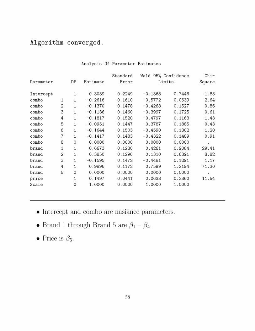
Algorithm converged.
Analysis Of Parameter Estimates
Standard Wald 95% Confidence Chi-
Parameter DF Estimate Error Limits Square
Intercept 1 0.3039 0.2249 -0.1368 0.7446 1.83
combo 1 1 -0.2616 0.1610 -0.5772 0.0539 2.64
combo 2 1 -0.1370 0.1478 -0.4268 0.1527 0.86
combo 3 1 -0.1136 0.1460 -0.3997 0.1725 0.61
combo 4 1 -0.1817 0.1520 -0.4797 0.1163 1.43
combo 5 1 -0.0951 0.1447 -0.3787 0.1885 0.43
combo 6 1 -0.1644 0.1503 -0.4590 0.1302 1.20
combo 7 1 -0.1417 0.1483 -0.4322 0.1489 0.91
combo 8 0 0.0000 0.0000 0.0000 0.0000 .
brand 1 1 0.6673 0.1230 0.4261 0.9084 29.41
brand 2 1 0.3850 0.1296 0.1310 0.6391 8.82
brand 3 1 -0.1595 0.1472 -0.4481 0.1291 1.17
brand 4 1 0.9896 0.1172 0.7599 1.2194 71.30
brand 5 0 0.0000 0.0000 0.0000 0.0000 .
price 1 0.1497 0.0441 0.0633 0.2360 11.54
Scale 0 1.0000 0.0000 1.0000 1.0000
• Intercept and combo are nusiance parameters.
• Brand 1 through Brand 5 are β1 – β4.
• Price is β5.
58

Now using PHREG.
The following program is basically from the SAS Logistic
Regression (1995) book, which is also pretty much the same as the
program in Kuhfeld (2001).
This section puts the data in the format needed for PROC PHREG:
data brands3;
set brands;
drop p1-p5 f1-f5;
* Define arrays for variables of the orginal data set;
array p[5] p1-p5; /* Array for prices*/
array f[5] f1-f5; /* Array for frequencies*/
* Define arrays for design matrices in new data set;
array pb[5] price1-price5; /* Array for prices*/
array brand[5] brand1-brand5; /* Aarray for brands*/;
* Initialize brand and brand by price design matrices;
do j=1 to 5; /* 5=number of choice options*/
brand[j]=0;
pb[j]=0;
end;
* Count the total number of choices;
nobs = sum(of f1-f5);
59

* Store choice set number to stratify;
ch_set=_n_;
* Create design matrix;
do j=1 to 5;
price = p[j];
brand[j]=1;
pb[j] = price;
* Output number of times each brand choosen;
freq = f[j];
choose=1;
t = 1; /* choice occurs at time 1 */
output;
* Output number of times each brand was not choosen;
freq = nobs-f[j];
choose =0;
t = 2; /* NON choice occurs at time 2 */
output;
* Set up for next alternative;
brand[j] = 0;
pb[j] = 0;
end;
run;
60

The data looks like:
p p p p p b b b b b c c
r r r r r r r r r r h p h
i i i i i a a a a a n _ r f o
O c c c c c n n n n n o s i r o
b e e e e e d d d d d b e c e s
s 1 2 3 4 5 1 2 3 4 5 j s t e q e t
1 5.99 0.00 0.00 0.00 0.00 1 0 0 0 0 1 100 1 5.99 12 1 1
2 5.99 0.00 0.00 0.00 0.00 1 0 0 0 0 1 100 1 5.99 88 0 2
3 0.00 5.99 0.00 0.00 0.00 0 1 0 0 0 2 100 1 5.99 19 1 1
4 0.00 5.99 0.00 0.00 0.00 0 1 0 0 0 2 100 1 5.99 81 0 2
5 0.00 0.00 5.99 0.00 0.00 0 0 1 0 0 3 100 1 5.99 22 1 1
6 0.00 0.00 5.99 0.00 0.00 0 0 1 0 0 3 100 1 5.99 78 0 2
7 0.00 0.00 0.00 5.99 0.00 0 0 0 1 0 4 100 1 5.99 33 1 1
8 0.00 0.00 0.00 5.99 0.00 0 0 0 1 0 4 100 1 5.99 67 0 2
9 0.00 0.00 0.00 0.00 4.99 0 0 0 0 1 5 100 1 4.99 14 1 1
10 0.00 0.00 0.00 0.00 4.99 0 0 0 0 1 5 100 1 4.99 86 0 2
11 5.99 0.00 0.00 0.00 0.00 1 0 0 0 0 1 100 2 5.99 34 1 1
12 5.99 0.00 0.00 0.00 0.00 1 0 0 0 0 1 100 2 5.99 66 0 2
13 0.00 5.99 0.00 0.00 0.00 0 1 0 0 0 2 100 2 5.99 26 1 1
14 0.00 5.99 0.00 0.00 0.00 0 1 0 0 0 2 100 2 5.99 74 0 2
15 0.00 0.00 3.99 0.00 0.00 0 0 1 0 0 3 100 2 3.99 8 1 1
The PHREG commands to fit the two models:
proc phreg data=brands3;
strata ch_set;
model t*choose(0)=brand1 brand2 brand3 brand4 brand5 price;
freq freq;
title ’PHREG: Discrete choice with common price effect’;
61

proc phreg data=brands3;
strata ch_set;
model t*choose(0)=brand1-brand5 price1-price5;
freq freq;
title ’PHREG: Discrete choice with brand by price effect’;
run;
A little edited output:
The PHREG Procedure
Model Information
Data Set WORK.BRANDS3
Dependent Variable t
Censoring Variable choose
Censoring Value(s) 0
Frequency Variable freq
Ties Handling BRESLOW
62

Summary of the Number of Event and Censored Values
Percent
Stratum ch_set Total Event Censored Censored
1 1 500 100 400 80.00
2 2 500 100 400 80.00
3 3 500 100 400 80.00
4 4 500 100 400 80.00
5 5 500 100 400 80.00
6 6 500 100 400 80.00
7 7 500 100 400 80.00
8 8 500 100 400 80.00
-------------------------------------------------------------------
Total 4000 800 3200 80.00
Convergence Status
Convergence criterion (GCONV=1E-8) satisfied.
Model Fit Statistics
Without With
Criterion Covariates Covariates
-2 LOG L 9943.373 9793.486
AIC 9943.373 9803.486
SBC 9943.373 9826.909
The PHREG Procedure
Analysis of Maximum Likelihood Estimates
63

Parameter Standard Hazard
Variable DF Estimate Error Chi-Square Pr > ChiSq Ratio
brand1 1 0.66727 0.12305 29.4065 <.0001 1.949
brand2 1 0.38503 0.12962 8.8235 0.0030 1.470
brand3 1 -0.15955 0.14725 1.1740 0.2786 0.853
brand4 1 0.98964 0.11720 71.2993 <.0001 2.690
brand5 0 0 . . . .
price 1 0.14966 0.04406 11.5379 0.0007 1.161
64

Example 3: From Powers & Xie (2000). n = 152 respondents.
The Response variable is mode of transportation:
j = 1 for train, 2 for bus, and 3 for car.
Explanatory Variables are:
tij = time waiting in Terminal.
vij = time spent in the Vehicle.
cij = Cost of time spent in vehicle.
gij = Generalized cost measure = cij + vij(valueij) where value
equals subjective value of respondent’s time for each mode of
transportation.
The multinomial logit model that appears to fit the data is
πij =exp[β1tij + β2vij + β3cij + β4gij]
∑3h=1 exp[β1tih + β2vih + β3cih + β4gih]
The odds of choosing mode j versus mode k for individual i,
πij
πik= exp[β1(tij−tik)] exp[β2(vij−vik)] exp[β3(cij−cik)] exp[β4(gij−gik)]
65
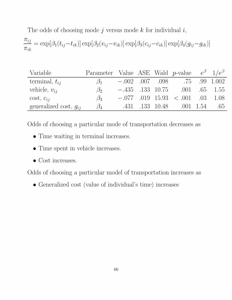
The odds of choosing mode j versus mode k for individual i,
πij
πik= exp[β1(tij−tik)] exp[β2(vij−vik)] exp[β3(cij−cik)] exp[β4(gij−gik)]
Variable Parameter Value ASE Wald p-value eβ 1/eβ
terminal, tij β1 −.002 .007 .098 .75 .99 1.002
vehicle, vij β2 −.435 .133 10.75 .001 .65 1.55
cost, cij β3 −.077 .019 15.93 < .001 .03 1.08
generalized cost, gij β4 .431 .133 10.48 .001 1.54 .65
Odds of choosing a particular mode of transportation decreases as
• Time waiting in terminal increases.
• Time spent in vehicle increases.
• Cost increases.
Odds of choosing a particular model of transportation increases as
• Generalized cost (value of individual’s time) increases
66

The Mixed Model
The conditional multinomial model that incorporates attributes of
the categories (choices) and of the decision maker.
This model is a combination of the multinomial and conditional
multinomial modela.
Suppose
• Response variable Y has J categories/levels.
• Explanatory variables
xi that is a measure of an attribute of individual i
wj that is a measure of an attribute of alternative j.
zij that is a measure of an attribute of alternative j for
individual i.
The “Mixed” Model:
πj(xi, wj, zij) =exp[αj + β1jxi + β2wj + β3zij]
∑Jh=1 exp[αh + β1hxi + β2wh + β3zih]
The odds of individual i choosing category j versus category k,
πj(xi, wj, zij)
πk(xi, wk, zik)= exp[αj − αk] exp[(β1j − β1k)xi]
exp[β2(wj − wk)] exp[β3(zij − zik)]
67
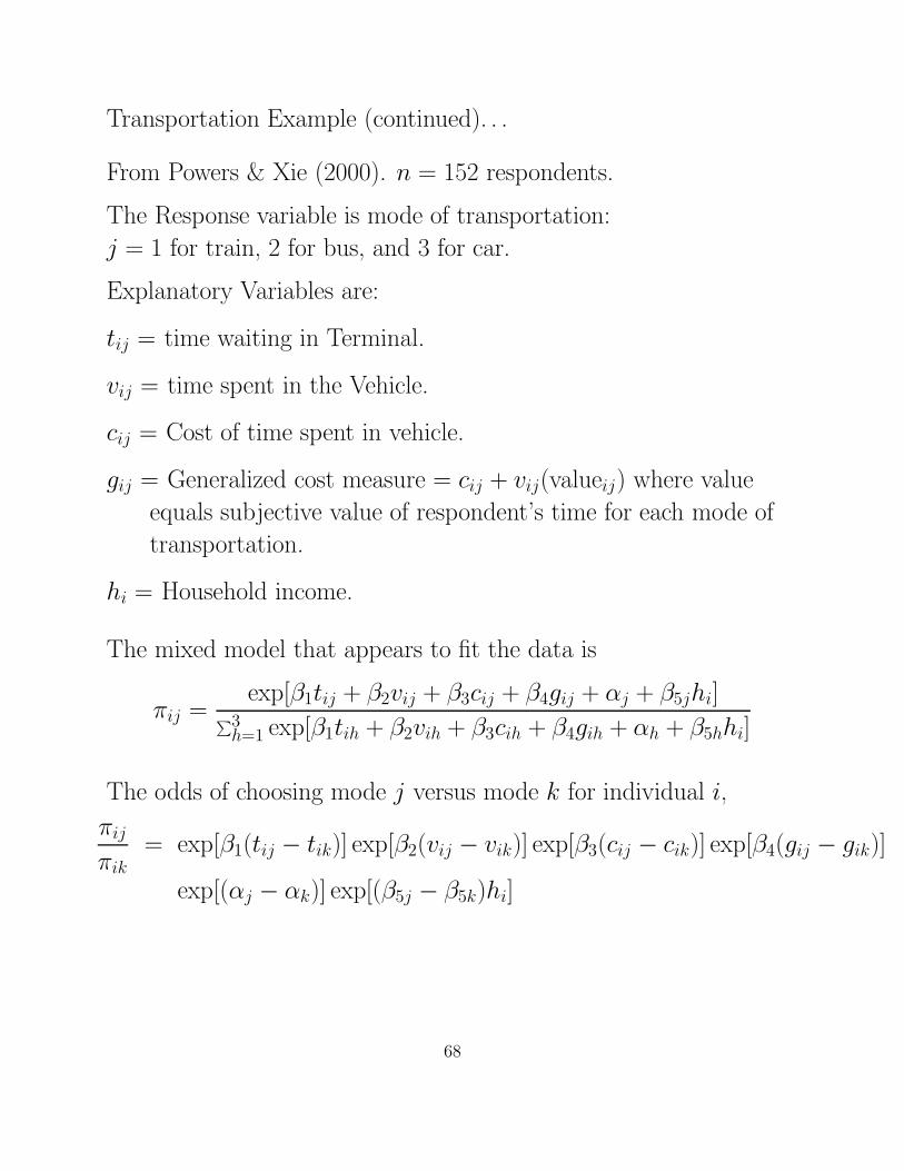
Transportation Example (continued). . .
From Powers & Xie (2000). n = 152 respondents.
The Response variable is mode of transportation:
j = 1 for train, 2 for bus, and 3 for car.
Explanatory Variables are:
tij = time waiting in Terminal.
vij = time spent in the Vehicle.
cij = Cost of time spent in vehicle.
gij = Generalized cost measure = cij + vij(valueij) where value
equals subjective value of respondent’s time for each mode of
transportation.
hi = Household income.
The mixed model that appears to fit the data is
πij =exp[β1tij + β2vij + β3cij + β4gij + αj + β5jhi]
∑3h=1 exp[β1tih + β2vih + β3cih + β4gih + αh + β5hhi]
The odds of choosing mode j versus mode k for individual i,
πij
πik= exp[β1(tij − tik)] exp[β2(vij − vik)] exp[β3(cij − cik)] exp[β4(gij − gik)]
exp[(αj − αk)] exp[(β5j − β5k)hi]
68

The odds of choosing mode j versus mode k for individual i,
πij
πik= exp[β1(tij − tik)] exp[β2(vij − vik)] exp[β3(cij − cik)] exp[β4(gij − gik)]
exp[(αj − αk)] exp[(β5j − β5k)hi]
Parameter Estimates:
Variable Parameter Value ASE Wald p-value eβ 1/eβ
Terminal, tij β1 −.074 .017 19.01 < .001 .93 1.08
Vehicle, vij β2 −.619 .152 16.54 < .001 .54 1.86
Cost, cij β3 −.096 .022 19.02 < .001 .91 1.10
Generalized cost, gij β4 .581 .150 15.08 < .001 1.79 .56
Bus
Intercept, α1 −2.108 .730 6.64 .01
Income, hi β51 .031 .021 1.97 .16 1.03 .97
Car
Intercept α2 −6.147 1.029 35.70 < .001
Income, hi β52 .048 .023 7.19 .01 1.05 .95
Effect of household income:
• The odds of choosing a bus versus a train given household
income increases from hi to hi + 100 unit is
exp(100(.031)) = 22.2 times larger.
• The odds of choosing a car versus a train given household
income increases from hi to hi + 100 unit is
exp(100(.048)) = 121.5 times larger.
69

• The odds of choosing a car versus a bus given household
income increases from hi to hi + 100 unit is
exp(100(.048 − .031)) = exp(1.7) = 5.5 times larger.
70

Logit Models for ordinal responses
Situation: Polytomous response and categories are ordered.
The logit model for this situation
• Use the ordering of the categories in forming logits.
• Yield simpler models with simpler interpretations than nominal
model.
• Is more powerful than nominal models.
Outline:
1. Cumulative logit model, or the “proportional odds” model.
2. Adjacent categories logit model.
3. Continuation ratio logits.
71

Cumulative Logit Model
Forming logits or how to dichotomize categories of Y such that
we incorporate the ordinal information.
Use Cumulative Probabilities:
Y = 1, 2, . . . , J and order is relavant.
{π1, π2, . . . , πJ}.
P (Y ≤ j) = π1 + . . . + πj =∑j
h=1 πh for j = 1, . . . , J − 1.
“Cumulative logits”
log
P (Y ≤ j)
P (Y > j)
= log
P (Y ≤ j)
1 − P (Y ≤ j)
= log
π1 + . . . + πj
πj+1 + . . . + πJ)
for j = 1, . . . , J − 1
The “Proportional Odds Model”
logit[P (Y ≤ j)] = log
P (Y ≤ j)
P (Y > j)
= αj+βx for j = 1, . . . , J−1
• αj (intercepts) can differ.
• β (slope) is constant.
– The effect of x is the same for all J − 1 ways to collapse Y
into dichotomous outcomes.
– A single parameter describes the effect of x on Y (versus
J − 1 in the baseline model).
72

• Interpretation in terms of odds ratios.
For a given level of Y (say Y = j)
P (Y ≤ j|X = x2)/P (Y > j|X = x2)
P (Y ≤ j|X = x1)/P (Y > J |X = x1)=
P (Y ≤ j|x2)P (Y > j|x1)
P (Y ≤ j|x1)P (Y > j|x2)
= exp(αj + βx2)/ exp(αj + βx1)
= exp[β(x2 − x1)]
or log odds ratio = β(x2 − x1).
The odds ratio is proportional to the difference (distance) between
x1 and x2 (this is sometimes referred to as “difference model”).
Since the proportionality = β is constant, this model is called the
“Proportional Odds Model”.
• Note that the cumulative probabilities are given by
P (Y ≤ j) =exp(αj + βx)
1 + exp(αj + βx)
Since β is constant, curves of cumulative probabilities plotted
against x are parallel.
• We can compute the probability of being in category j by
taking differences between the cumulative probabilities.
P (Y = j) = P (Y ≤ j) − P (Y ≤ j − 1) for j = 2, . . . , J
and
P (Y = 1) = P (Y ≤ 1)
73

Since β is constant, these probabilities are guaranteed to be
non-negative.
• In fitting this model to data, it must be simultaneous.
In SAS
– LOGISTIC (maximum likelihood).
– CATMOD (weighted least squares).
For larger samples with categorical explanatory variables, the
results are almost the same.
74
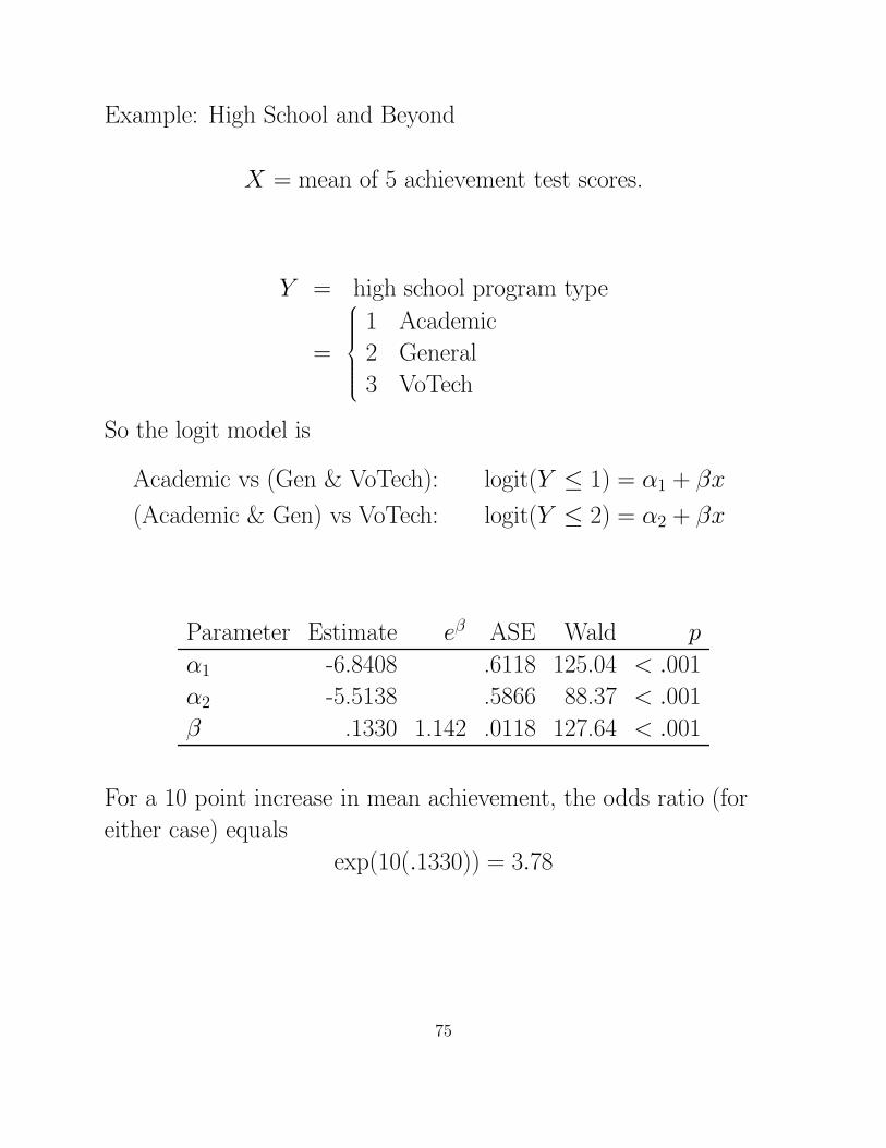
Example: High School and Beyond
X = mean of 5 achievement test scores.
Y = high school program type
=
1 Academic
2 General
3 VoTech
So the logit model is
Academic vs (Gen & VoTech): logit(Y ≤ 1) = α1 + βx
(Academic & Gen) vs VoTech: logit(Y ≤ 2) = α2 + βx
Parameter Estimate eβ ASE Wald p
α1 -6.8408 .6118 125.04 < .001
α2 -5.5138 .5866 88.37 < .001
β .1330 1.142 .0118 127.64 < .001
For a 10 point increase in mean achievement, the odds ratio (for
either case) equals
exp(10(.1330)) = 3.78
75
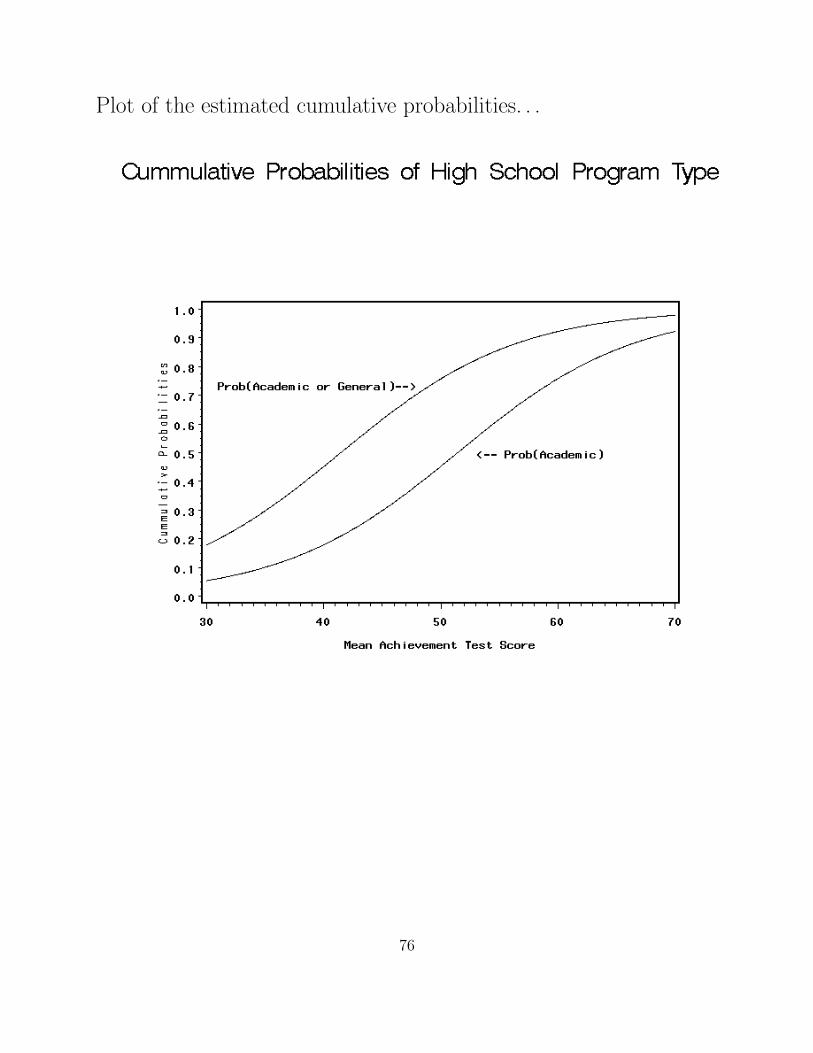
Plot of the estimated cumulative probabilities. . .
76
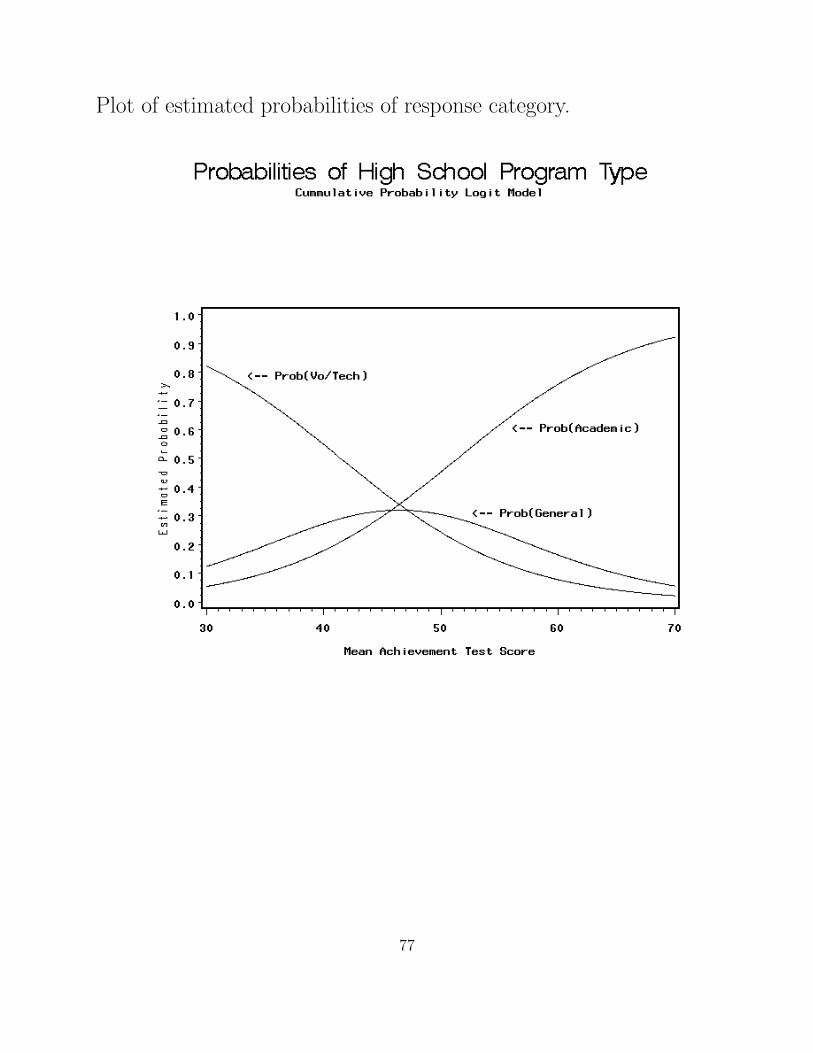
Plot of estimated probabilities of response category.
77

In the example, we would get the exact same results regarding
interpretation if we had used
Y = high school program type
=
1 VoTech
2 General
3 Academic
This reversal of the ordering of Y would
• Change the signs of the estimated parameters.
• Yield curves of cumulative probabilities that decrease (rather
than increase).
SAS code for the example presented:
PROC LOGISTIC;
MODEL hsp = achieve;
Fitting the cumulative logit model is the default if the response
variables has more than 2 categories.
78

Final Comments on Cumulative Logit Models
Nice things about proportional odds model:
• It takes into account the ordering of the categories of the
response variable.
• P(Y=1) is monotonically increasing as a function of x.
(see figure of estimated probabilities).
• P(Y=J) is monotonically decreasing as a function of x.
(see figure of estimated probabilities).
• Curves of probabilities for intermediate categories are
uni-modal with the modes (maximum) corresponding to the
order of the categories.
• The conclusions regarding the relationship between Y and x
are not affected by the response category.
The specific combination of categories examined does not lead
to substantially difference conclusions regarding the
relationship between responses and x.
If the proportional odds model does not fit well, then you can use
the baseline (nominal) model and use the ordering of the responses
in your interpretation of the model. For other possibilities, see Long
(1997).
IRT connection: Samejima’s (1969) graded response model for
polytomous items is the same as the proportional odds model
except that x is a latent continuous variable.
79
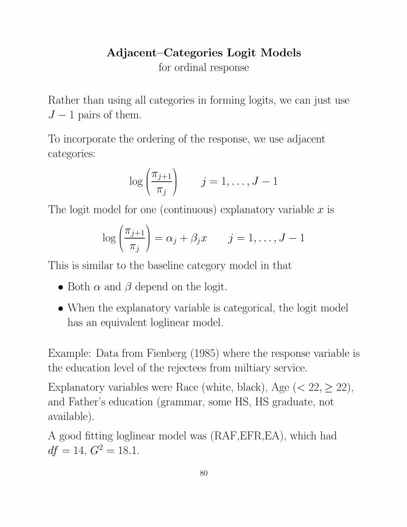
Adjacent–Categories Logit Models
for ordinal response
Rather than using all categories in forming logits, we can just use
J − 1 pairs of them.
To incorporate the ordering of the response, we use adjacent
categories:
log
πj+1
πj
j = 1, . . . , J − 1
The logit model for one (continuous) explanatory variable x is
log
πj+1
πj
= αj + βjx j = 1, . . . , J − 1
This is similar to the baseline category model in that
• Both α and β depend on the logit.
• When the explanatory variable is categorical, the logit model
has an equivalent loglinear model.
Example: Data from Fienberg (1985) where the response variable is
the education level of the rejectees from miltiary service.
Explanatory variables were Race (white, black), Age (< 22,≥ 22),
and Father’s education (grammar, some HS, HS graduate, not
available).
A good fitting loglinear model was (RAF,EFR,EA), which had
df = 14, G2 = 18.1.
80
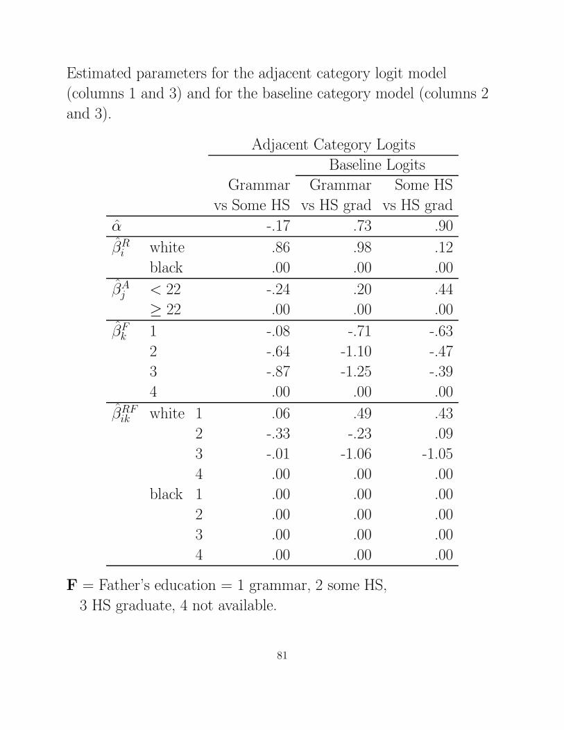
Estimated parameters for the adjacent category logit model
(columns 1 and 3) and for the baseline category model (columns 2
and 3).
Adjacent Category Logits
Baseline Logits
Grammar Grammar Some HS
vs Some HS vs HS grad vs HS grad
α̂ -.17 .73 .90
β̂Ri white .86 .98 .12
black .00 .00 .00
β̂Aj < 22 -.24 .20 .44
≥ 22 .00 .00 .00
β̂Fk 1 -.08 -.71 -.63
2 -.64 -1.10 -.47
3 -.87 -1.25 -.39
4 .00 .00 .00
β̂RFik white 1 .06 .49 .43
2 -.33 -.23 .09
3 -.01 -1.06 -1.05
4 .00 .00 .00
black 1 .00 .00 .00
2 .00 .00 .00
3 .00 .00 .00
4 .00 .00 .00
F = Father’s education = 1 grammar, 2 some HS,
3 HS graduate, 4 not available.
81
A simpler logit model for adjacent categories:
log
πj+1
πj
= αj + βx j = 1, . . . , J − 1
This is similar to the cummulative logit model in that the effect of
x on Y is constant across logit (in this case, pairs of categories).
For two categories (say Y=1 and Y=4), the effect of x equals
β(4 − 1)
If you have just 1 categorical variable,
• The more complex adjacent categories logit model with βj and
the corresponding loginear model are saturated.
• The simpler model with β constant is not saturated.
The simpler model is equvialent to a loglinear with linear by linear
term for the relationship between the explanatory and response
variables.
82
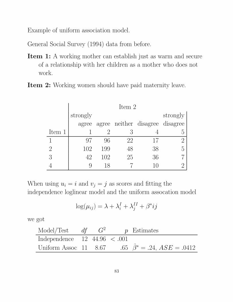
Example of uniform association model.
General Social Survey (1994) data from before.
Item 1: A working mother can establish just as warm and secure
of a relationship with her children as a mother who does not
work.
Item 2: Working women should have paid maternity leave.
Item 2
strongly strongly
agree agree neither disagree disagree
Item 1 1 2 3 4 5
1 97 96 22 17 2
2 102 199 48 38 5
3 42 102 25 36 7
4 9 18 7 10 2
When using ui = i and vj = j as scores and fitting the
independence loglinear model and the uniform assocation model
log(µij) = λ + λIi + λII
j + β∗ij
we got
Model/Test df G2 p Estimates
Independence 12 44.96 < .001
Uniform Assoc 11 8.67 .65 β̂∗ = .24, ASE = .0412
83
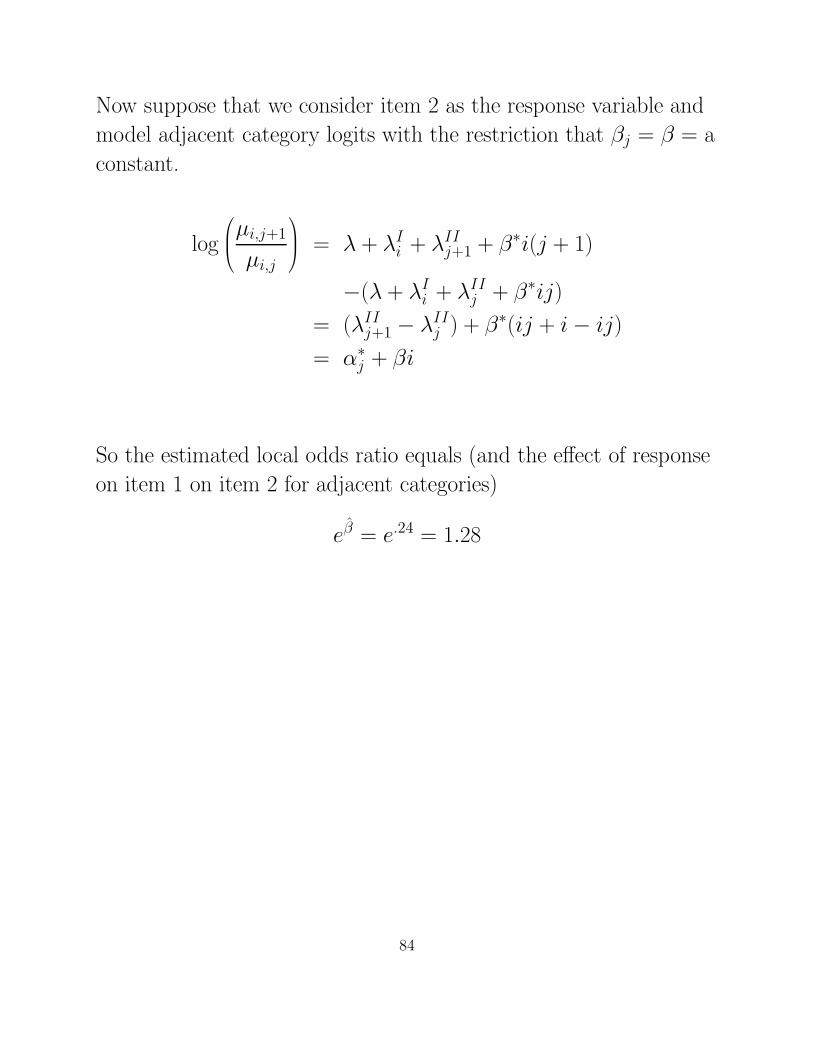
Now suppose that we consider item 2 as the response variable and
model adjacent category logits with the restriction that βj = β = a
constant.
log
µi,j+1
µi,j
= λ + λI
i + λIIj+1 + β∗i(j + 1)
−(λ + λIi + λII
j + β∗ij)
= (λIIj+1 − λII
j ) + β∗(ij + i − ij)
= α∗j + βi
So the estimated local odds ratio equals (and the effect of response
on item 1 on item 2 for adjacent categories)
eβ̂ = e.24 = 1.28
84

Continuation–Ratio Logits
for ordinal responses
In this approach, the order of the categories of the response variable
is incorporated by forming a series of (J − 1) logits
log
π1
π2
, log
π1 + π2
π3
, . . . , log
π1 + . . . + πJ−1
πJ
or
log
π1
π2 + . . . + πJ
, log
π2
π3 + . . . + πJ
, . . . , log
πJ−1
πJ
These are called “continuation–ratio logits”.
When the models have different parameters for each logit, e.g.,
αj + βjx
• Just apply regular binary logistic regression to each one.
• The fitting can be separate.
• The sum of the separate df and G2 provide an overall global
goodness of fit test and measure (same as simultaneous fitting).
85
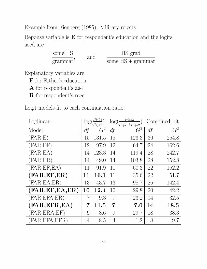
Example from Fienberg (1985): Military rejects.
Reponse variable is E for respondent’s education and the logits
used are
some HS
grammar, and
HS grad
some HS + grammar
Explanatory variables are
F for Father’s education
A for respondent’s age
R for respondent’s race.
Logit models fit to each continuation ratio:
Loglinear log(µijk1µijk2
) log(µijk3
µijk1+µijk2) Combined Fit
Model df G2 df G2 df G2
(FAR,E) 15 131.5 15 123.3 30 254.8
(FAR,EF) 12 97.9 12 64.7 24 162.6
(FAR,EA) 14 123.3 14 119.4 28 242.7
(FAR,ER) 14 49.0 14 103.8 28 152.8
(FAR,EF,EA) 11 91.9 11 60.3 22 152.2
(FAR,EF,ER) 11 16.1 11 35.6 22 51.7
(FAR,EA,ER) 13 43.7 13 98.7 26 142.4
(FAR,EF,EA,ER) 10 12.4 10 29.8 20 42.2
(FAR,EFA,ER) 7 9.3 7 23.2 14 32.5
(FAR,EFR,EA) 7 11.5 7 7.0 14 18.5
(FAR,ERA,EF) 9 8.6 9 29.7 18 38.3
(FAR,EFA,EFR) 4 8.5 4 1.2 8 9.7
86

Notes:
• The best fitting loglinear model, which we could use for
baseline or adjacent categories model is
(FAR,EFR,EA)
which has df = 14, G2 = 18.5, p = .18 for the combined fit,
and for each separate logits
df = 7, G2 = 11.5, p = .12 and df = 7, G2 = 7.0, p = .43.
• We can find simpler models that fit for the logit comparing
Some HS and Grammar School:
(FAR,EF,EA,ER) with df = 10, G2 = 12.4, p = .23
(FAR,EF,ER) with df = 11, G2 = 16.1, p = .14.
The likelihood ratio statistic for Ho : λEAjl = 0 equals
G2 = 16.1 − 12.4 = 3.7 with df = 1, has p = .05.
The simpler of these two models states that given that the
respondent did not complete high school, the odds of their
completing some high school depends only on race and on their
father’s education.
The odds that a respondent completes high school requires a more
complex model.
87