Embed Size (px)
Citation preview
DOT Grant No. DTRT06-G-0044
Final Report
Performing OrganizationUniversity Transportation Center for Mobility™Texas Transportation InstituteThe Texas A&M University SystemCollege Station, TX
Sponsoring AgencyDepartment of TransportationResearch and Innovative Technology AdministrationWashington, DC
Improving the Quality of Life by Enhancing Mobility
University Transportation Center for Mobility™
The Value of Public Transportation for Improving the Quality of Life for the Rural Elderly
James W. Mjelde, Rebekka Dudensing, Linda K. Cherrington, Yanhong Jin, Alicia A. Israel, and Junyi Chen
UTCM Project #11-08-74July 2012
Technical Report Documentation Page 1. Report No. UTCM 11-08-74
2. Government Accession No.
3. Recipient's Catalog No.
4. Title and Subtitle THE VALUE OF PUBLIC TRANSPORTATION FOR IMPROVING THE QUALITY OF LIFE FOR THE RURAL ELDERLY
5. Report Date July 2012
6. Performing Organization Code Texas Transportation Institute
7. Author(s) James W. Mjelde, Rebekka Dudensing, Linda K. Cherrington, Yanhong Jin, Alicia A. Israel, and Junyi Chen
8. Performing Organization Report No. UTCM 11-08-74
9. Performing Organization Name and Address University Transportation Center for Mobility™ Texas Transportation Institute The Texas A&M University System 3135 TAMU College Station, TX 77843-3135
10. Work Unit No. (TRAIS) 11. Contract or Grant No. DTRT06-G-0044
12. Sponsoring Agency Name and Address Department of Transportation Research and Innovative Technology Administration 400 7th Street, SW Washington, DC 20590
13. Type of Report and Period Covered Final Report 01.01.11–05.31.12 14. Sponsoring Agency Code
15. Supplementary Notes Supported by a grant from the US Department of Transportation, University Transportation Centers Program 16. Abstract Transportation for the rural elderly is an increasing concern as baby boomers age and young people continue to exit rural communities. As the elderly are no longer able to drive themselves, they rely on alternate forms of transportation, including public transportation systems. However, such systems are often not a good substitute for driving a private car, especially in rural areas. This study focuses on non-medical transportation; medical transportation is addressed in the literature and is more widely available to the elderly. Because expanded rural transportation systems likely will be funded by taxpayers, an understanding of their preferences and willingness-to-pay for non-medical transportation options is essential. To fulfill this objective, a choice experiment survey was administered to taxpayers in three counties (Atascosa, Polk, and Parker) in Texas and to students at Texas A&M University. Results indicate that taxpayers value transportation services for the elderly and are willing to support them. They value more flexible options over base levels of the attributes presented, but they may not always prefer the most flexible options. Respondents’ willingness to pay for attributes was similar across counties, but differences in socio-demographic coefficients suggests that transportation systems may need to be customized to meet local needs. Furthermore, the cost of improvements to the transportation systems may be more than county residents are willing to pay. Students’ willingness-to-pay was generally higher than that of county residents, and the variation in students’ willingness to pay was smaller. However, students and county residents ranked the value of transportation attributes similarly, suggesting that students may be a good convenience sample for behavioral questions but less so for policy matters.
17. Key Word Public transportation, Rural elderly, Willingness-to-pay, Choice model
18. Distribution Statement Public distribution
19. Security Classif. (of this report) Unclassified
20. Security Classif. (of this page) Unclassified
21. No. of Pages 134
22. Price n/a
Form DOT F 1700.7 (8-72) Reproduction of completed page authorized
THE VALUE OF PUBLIC TRANSPORTATION FOR IMPROVING THE QUALITY OF LIFE FOR THE RURAL ELDERLY
By
James W. Mjelde (PI)
Professor Department of Agricultural Economics,
Texas A&M University [email protected]
Rebekka Dudensing Assistant Professor
Department of Agricultural Economics, Texas AgriLife Extension,
The Texas A&M University System [email protected]
Linda K. Cherrington
Program Manager and Research Scientist Texas Transportation Institute¸
The Texas A&M University System [email protected]
Yanhong Jin Assistant Professor
Department of Agricultural, Food and Resource Economics,
Rutgers University [email protected]
Alicia A. Israel M.S. Student
Department of Agricultural Economics, Texas AgriLife Extension,
The Texas A&M University System [email protected]
Junyi Chen
M.S. Student Department of Agricultural Economics,
Texas AgriLife Extension, The Texas A&M University System
UTCM Final Report Project Title: “The Value of Non-Medical Transportation for Improving the Quality of Life
for the Rural Elderly: Methodology and Information Considerations” Project #11-08-74
University Transportation Center for Mobility™ Texas Transportation Institute
The Texas A&M University System College Station, TX 77843-3135
July 2012
2
DISCLAIMER The contents of this report reflect the views of the authors, who are responsible for the facts and the accuracy of the information presented herein. This document is disseminated under the sponsorship of the Department of Transportation, University Transportation Centers Program in the interest of information exchange. The U.S. Government assumes no liability for the contents or use thereof.
ACKNOWLEDGEMENT Support for this research was provided by a grant from the U.S. Department of Transportation, University Transportation Centers Program to the University Transportation Center for Mobility™ (UTCM 11-08-74).
3
TABLE OF CONTENTS
List of Figures ................................................................................................................................ 5 List of Tables ................................................................................................................................. 6 Executive Summary ...................................................................................................................... 7 Chapter 1. Introduction ............................................................................................................... 9 Chapter 2. Literature Review .................................................................................................... 10
Background – Elderly Population of the U.S. and Texas ......................................................... 10 Mobility and the Elderly ........................................................................................................... 14
Chapter 3. Methodology and Survey Design ............................................................................ 19
Questionnaire Design ................................................................................................................ 19 Survey Questionnaire Design ................................................................................................... 22 Data Collection ......................................................................................................................... 24 The Random Utility Model and Model Specification ............................................................... 24
Chapter 4. Findings – Surveys in Atascosa and Polk Counties .............................................. 31
Respondents’ Demographic Characteristics – Atascosa County .............................................. 31 Respondents’ Demographic Characteristics – Polk County ..................................................... 34 Model Estimation ...................................................................................................................... 37 Differences between the Conditional Logit and Mixed Logit Models ..................................... 52
Chapter 5. Findings – Parker County Survey .......................................................................... 52
Respondents’ Demographic Characteristics – Parker County .................................................. 52 Model Estimation ...................................................................................................................... 57 Differences between the Conditional Logit and Mixed Logit Models ..................................... 63 Differences among the Three Counties..................................................................................... 63
Chapter 6. Findings – Student Survey ...................................................................................... 64
Students’ Demographic Characteristics .................................................................................... 64 Model Estimation ...................................................................................................................... 69 Differences between the Conditional Logit and Mixed Logit Models ..................................... 83
Chapter 7. Findings – Population and Individual Willingness-to-Pay Comparisons ........... 83
Conditional Logit WTP Comparisons ...................................................................................... 83 Mixed Logit WTP Comparisons ............................................................................................... 86
Chapter 8. Conclusions ............................................................................................................... 96
Transportation Preferences and Willingness-to-Pay ................................................................. 97 Comparison of Results between Counties ................................................................................ 98 Comparison of Results between Students and County Residents ............................................. 98 Mixed Logit versus Conditional Logit Estimation ................................................................... 99 Limitations and Future Research .............................................................................................. 99
Chapter 9. Implications ............................................................................................................ 101 References .................................................................................................................................. 103 Appendix A. County Resident Survey .................................................................................... 111 Appendix B. Student Survey .................................................................................................... 125

4
5
LIST OF FIGURES Figure 1. Distribution of Texas Elderly Population by Gender ................................................... 11 Figure 2. Distribution of Texas Elderly by Age Grouping .......................................................... 12 Figure 3. Percentage of Each Age Group among the Elderly Cohort .......................................... 12 Figure 4. Conditional Logit Model Population Mean WTP for the Specified Transportation Attribute over the Base Level ....................................................................................................... 86 Figure 5. Mixed Logit Model Population Mean WTP for the Specified Transportation Attribute over the Base Level ....................................................................................................................... 90 Figure 6. Percent of Population with a Positive Willingness to Pay ........................................... 91 Figure 7. WTP Distributions for the Transportation Options ...................................................... 92 Note: Color figures in this report may not be legible if printed in black and white. A color PDF copy of this report may be accessed via the UTCM website at http://utcm.tamu.edu, the Texas Transportation Institute website at http://tti.tamu.edu, or the Transportation Research Board’s TRID database at http://trid.trb.org.
6
LIST OF TABLES
Table 1. Example of a Transportation Option Choice Set ............................................................ 23 Table 2. Random Scenario Draw Information .............................................................................. 23 Table 3. Demographic Characteristics – Atascosa County ........................................................... 32 Table 4. Likert Scale Responses – Atascosa County .................................................................... 34 Table 5. Demographic Characteristics – Polk County .................................................................. 35 Table 6. Likert Scale Responses – Polk County ........................................................................... 37 Table 7. Variables used in Logit Models – Atascosa and Polk Counties ..................................... 39 Table 8. Conditional Logit Model Results – Atascosa County .................................................... 41 Table 9. Mixed Logit Model Results – Atascosa County ............................................................. 42 Table 10. Conditional Logit Model Results – Polk County ......................................................... 44 Table 11. Mixed Logit Model Results – Polk County .................................................................. 45 Table 12. Summary Statistics for Conditional and Mixed Logit Models – Atascosa and Polk Counties ........................................................................................................................................ 46 Table 13. Chi-Squared Hypothesis Tests – Atascosa and Polk Counties ..................................... 47 Table 14. Demographic Characteristics – Parker County ............................................................. 54 Table 15. Likert Scale Responses – Parker County ...................................................................... 56 Table 16. Conditional Logit Model Results – Parker County ...................................................... 58 Table 17. Mixed Logit Model Results – Parker County ............................................................... 59 Table 18. Summary Statistics for Conditional and Mixed Logit Models – Parker ....................... 60 Table 19. Chi-Squared Hypothesis Tests – Parker County........................................................... 60 Table 20. Demographic Characteristics – Student ........................................................................ 65 Table 21. Likert Scale Responses – 2011 Student ........................................................................ 67 Table 22. Likert Scale Responses – Student 2012 ........................................................................ 69 Table 23. Variables used in Logit Models - Student .................................................................... 71 Table 24. Conditional Logit Model Results – 2011 Student ........................................................ 72 Table 25. Conditional Logit Model Results – 2012 Student ........................................................ 73 Table 26. Mixed Logit Model Results – 2011 Student ................................................................. 74 Table 27. Mixed Logit Model Results – Student 2012 ................................................................. 76 Table 28. Summary Statistics for Conditional and Mixed Logit Models – 2011 Student ............ 77 Table 29. Summary Statistics for Conditional and Mixed Logit Models – 2012 Student ............ 77 Table 30. Chi-Squared Hypothesis Tests – 2011 Student ............................................................. 78 Table 31. Chi-Squared Hypothesis Tests – Student 2012............................................................. 78 Table 32. Comparisons of the Conditional Logit Model WTP ..................................................... 84 Table 33. Comparisons of the Mixed Logit Model WTP ............................................................. 88 Table 34. Wilcoxon-Mann-Whitney Rank-Sum Tests ................................................................. 94
7
EXECUTIVE SUMMARY
Mobility is an undeniable issue for current and future elderly populations. The increasing popularity for retirees to live in rural communities makes this a particularly important issue in rural areas. When an elderly individual living in a rural community is no longer able to drive, issues that come with living in a rural area may be exacerbated, and the individual may experience a decrease in their quality of life. Although individuals may be able to use public transportation most existing options do not promote an independent lifestyle. Any updated rural transportation system benefiting the elderly would be funded by taxpayers. An understanding of the taxpayers’ preferences and willingness-to-pay (WTP) for transportation options, therefore, is essential. Few, if any economic studies have addressed this issue. The objectives of this research are to: (1) estimate economic WTP for public transportation options by using choice modeling techniques; and (2) better understand opinions related to public transportation for the elderly held by the general population as a whole and within different demographics. To complete these objectives, a choice survey was distributed to samples of three populations: residents of Atascosa County (located in south Texas); residents of Polk County (located in east Texas); residents of Parker County (located in north central Texas); and students at Texas A&M University. Respondents were presented with transportation options made of five attributes: addition to annual vehicle registration fee, days of operation, hours of operation, type of route, and senior citizen transportation fare discount. Results show both students and the general public value public transportation options and are willing to pay for specific transportation attributes. Respondents tended to prefer options that are more flexible than the less flexible attribute presented to them; however, respondents did not necessarily prefer the most flexible options. Students, generally, are willing to pay more for transportation attributes than county residents.
Overall, Atascosa, Polk, and Parker County residents have similar WTP, indicating both populations value rural public transportation similarly. The effects of socio-demographic variables on residents’ decision to choose a transportation option appear to differ between the counties. These findings imply that while the influence of transportation attribute levels are consistent across counties, local input is important in customizing transportation systems to meet local expectations.
From a policy makers’ standpoint, the results indicate support for improved transportation for the rural elderly. Further, the similarity of the WTP may indicate that there may be statewide support for rural transportation programs. The results also provide evidence that county residents’ willingness to pay may not provide sufficient revenue to pay for enhanced transportation services. For example, the mean WTP for a seven days a week service (over Monday, Wednesday, Friday service) in Atascosa County is $6.59. Across 14,500 registered vehicles, the county could generate an additional $96,555. It is not certain that that amount would pay for an expansion to seven days a week service. At the same time, local revenue could provide a match for additional grant funding.
8
While county residents valued transportation options, most residents were not familiar with their local transportation district. Even among people who were aware of the service, many did not know details about fares and scheduling. Transportation districts may find it beneficial to publicize their services to potential clientele.
Finally, the findings of this project suggest that students’ responses may be appropriate for making general inferences about attitudes, but students may not be an appropriate sample for use in implementing specific policy issues. Thus, the purpose of the study remains an important component to consider when selecting a sample.
9
CHAPTER 1. INTRODUCTION
Texas has one of the largest elderly1 populations in the country (He et al. 2005); this population is expected to increase in the coming decades (Texas State Demographer 2008). In 2009, nearly 25 percent of Texans over the age of 65 lived in rural areas (U.S. Census Bureau 2009). Living in rural towns or in the countryside will continue to be popular among current and future elderly cohorts (Cromartie and Nelson 2009). Therefore, it is necessary for Texas’ rural community developers to consider this age group when planning for the future, especially because maintaining a high quality of life can be challenging for residents of rural communities. Specifically, transportation issues are consistently mentioned by researchers as integral to the quality of life for rural senior citizens (Glasgow and Blakely 2000; Grant and Rice 1983). Although driving a private vehicle well into retirement is popular among rural Texans, studies have shown that this is not always the most feasible or safest option for elderly individuals (Burns 1999; Glasgow and Blakely 2000; Rosenbloom 2004 and 2009). There are limited rural public transportation options in Texas. The options that do exist, generally, do not promote an independent lifestyle if used as a primary form of transportation for daily activities (Foster et al. 1996; Glasgow and Blakely 2000; Mattson 2011; Rosenbloom 2004 and 2009). An elderly individual living in the country or a rural community who loses the ability to drive might suffer from isolation and a lower quality of life. Public transportation that supports elderly individuals is an important issue for rural developers to consider in creating an aging friendly community.
This research estimates the willingness-to-pay of Texas county residents and students for transportation options that support the rural elderly. An updated rural transportation system would most likely need to be funded by taxpayers, so an understanding of their preferences and willingness-to-pay for transportation options is essential. The objectives of this research are:
(1) estimate economic willingness-to-pay for various public transportation options by using choice modeling techniques, namely, conditional, and mixed logit estimation; and (2) better understand opinions related to public transportation for the elderly held by the general population as a whole and within different demographics.
Specific questions that will be addressed include but are not limited to:
• Would a taxpayer be willing to pay for transportation services? • Do older individuals prefer different transportation options more than younger
individuals? • Would those who have children living far away from their home be willing to pay
more than those whose children live close to their home?
To achieve these objectives, Texas county residents and students were surveyed. Using both of these groups is important because an updated rural transportation system would affect county 1 In this thesis, the terms ‘elderly,’ ‘senior citizens,’ ‘elderly population,’ ‘elderly cohort,’ etc. refer to those who are 65 years of age or older.
10
residents sooner than students, but undergraduate students will pay for the updates longer than many current county residents. By meeting these objectives, a better understanding of who would be willing to pay and how much they are willing to pay for which type of transportation options is obtained. This research contributes to the current literature on elderly mobility by addressing non-emergency mobility issues. Previous studies have focused on the general or metropolitan elderly population and the availability of medical transportation. Transportation for medical reasons is generally more accessible for senior citizens than transportation to go shopping or attend community and social functions. Although medical transportation is not to be excluded from this research, the focus is on transportation options that support the non-medical needs of the elderly.
CHAPTER 2. LITERATURE REVIEW
BACKGROUND – ELDERLY POPULATION OF THE U.S. AND TEXAS The high birth rates sustained by the economic prosperity and family-friendly government programs immediately following World War II gave rise to the Baby Boomers, one of the largest generations in U.S. history (U.S. Census Bureau 2006). Demographics in the U.S. are showing the effects of the Baby Boomer cohort. For example in 1990, just before Baby Boomers began to reach middle-age, only 42 million people or 17 percent of the population were in their middle-age years (Cromartie and Nelson 2009). By 2009, there were 83 million Baby Boomers between the ages of 45 and 63, approximately 28 percent of the U.S. population (Cromartie and Nelson 2009). Because this cohort represents a large, diverse portion of the U.S. population, Baby Boomers have been the subject of considerable research as they have matured (Rosenbloom 1993; U.S. Department of Agriculture 2007). As Baby Boomers have reached retirement age, research has turned to determining how current social programs may need to be adjusted to accommodate this population cohort (Alsnih and Hensher 2003; Cromartie and Nelson 2009; U.S. Department of Agriculture 2007). Elderly Population The elderly population is increasing and will continue to do so as Baby Boomers age and the elderly live longer, healthier lives (He et al. 2005; Rosenbloom 2004). In 2009, 39.6 million Americans, or 12.9 percent of the total population, were over age 65, with approximately 5.6 million (1.8 percent) over age 85 (U.S. Census Bureau 2009). The U.S. Census Bureau (2008) projected that the elderly cohort will increase to approximately 55 million by 2020. Rosenbloom (2004, p. 2) states:
Most of the elderly will be in good health and not seriously disabled. In fact disability rates have been falling among all cohorts of the elderly for decades, owing to a combination of good nutrition, improved health care, better education and higher incomes…Although disability rates increase with age, two-thirds of those over age 85 reported being in good to excellent health. Overall, new generations of older Americans will be healthier for a greater percentage of their lives than those just a few decades ago.
11
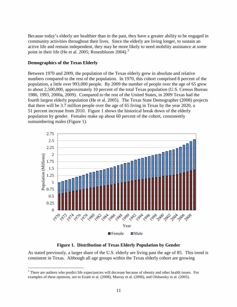
Because today’s elderly are healthier than in the past, they have a greater ability to be engaged in community activities throughout their lives. Since the elderly are living longer, to sustain an active life and remain independent, they may be more likely to need mobility assistance at some point in their life (He et al. 2005; Rosenbloom 2004).2 Demographics of the Texas Elderly Between 1970 and 2009, the population of the Texas elderly grew in absolute and relative numbers compared to the rest of the population. In 1970, this cohort comprised 8 percent of the population, a little over 993,000 people. By 2009 the number of people over the age of 65 grew to about 2,500,000, approximately 10 percent of the total Texas population (U.S. Census Bureau 1986, 1993, 2000a, 2009). Compared to the rest of the United States, in 2009 Texas had the fourth largest elderly population (He et al. 2005). The Texas State Demographer (2008) projects that there will be 3.7 million people over the age of 65 living in Texas by the year 2020, a 51 percent increase from 2010. Figure 1 shows the historical break down of the elderly population by gender. Females make up about 60 percent of the cohort, consistently outnumbering males (Figure 1).
Figure 1. Distribution of Texas Elderly Population by Gender
As stated previously, a larger share of the U.S. elderly are living past the age of 85. This trend is consistent in Texas. Although all age groups within the Texas elderly cohort are growing
2 There are authors who predict life expectancies will decrease because of obesity and other health issues. For examples of these opinions, see to Ezatti et al. (2008), Murray et al. (2006), and Olshansky et al. (2005).
00.250.5
0.751
1.251.5
1.752
2.252.5
2.75
Popu
latio
n (M
illio
ns)
Year
Female Male
12
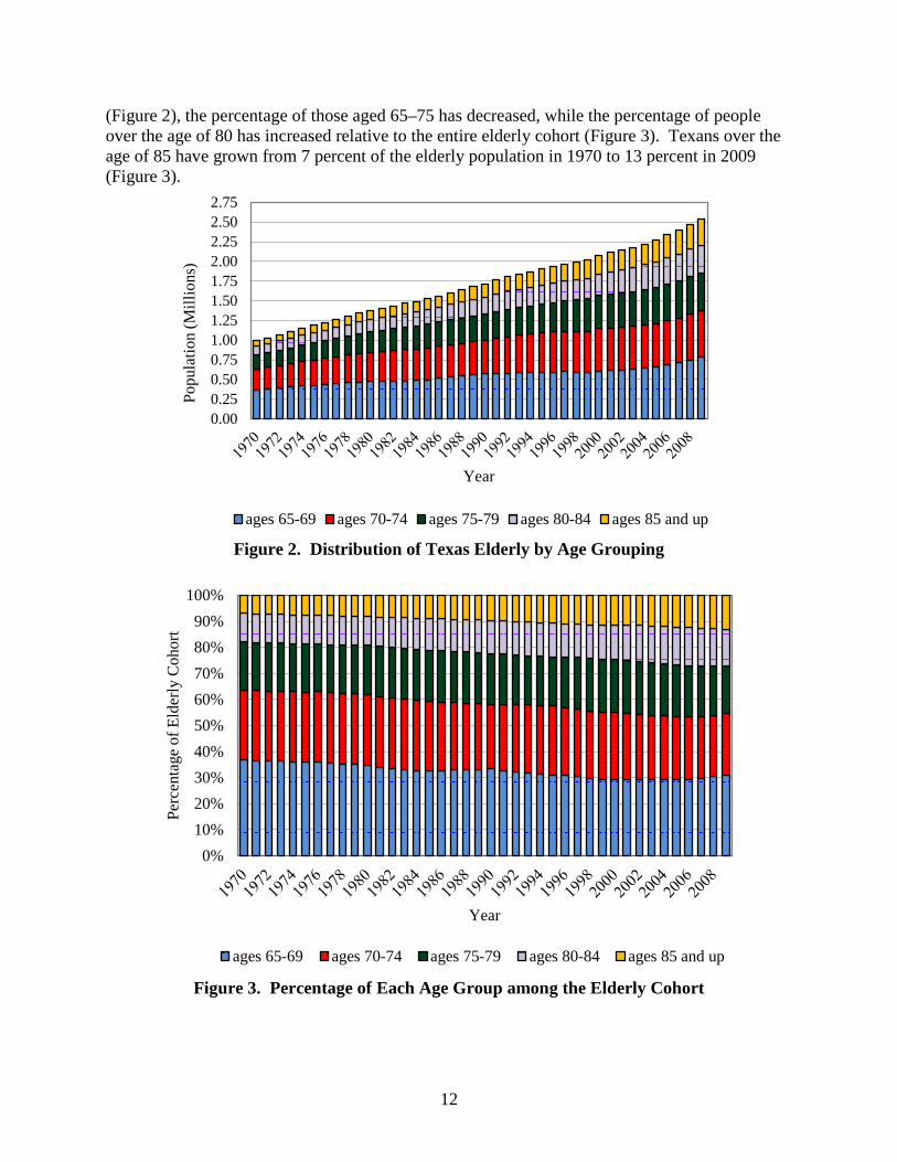
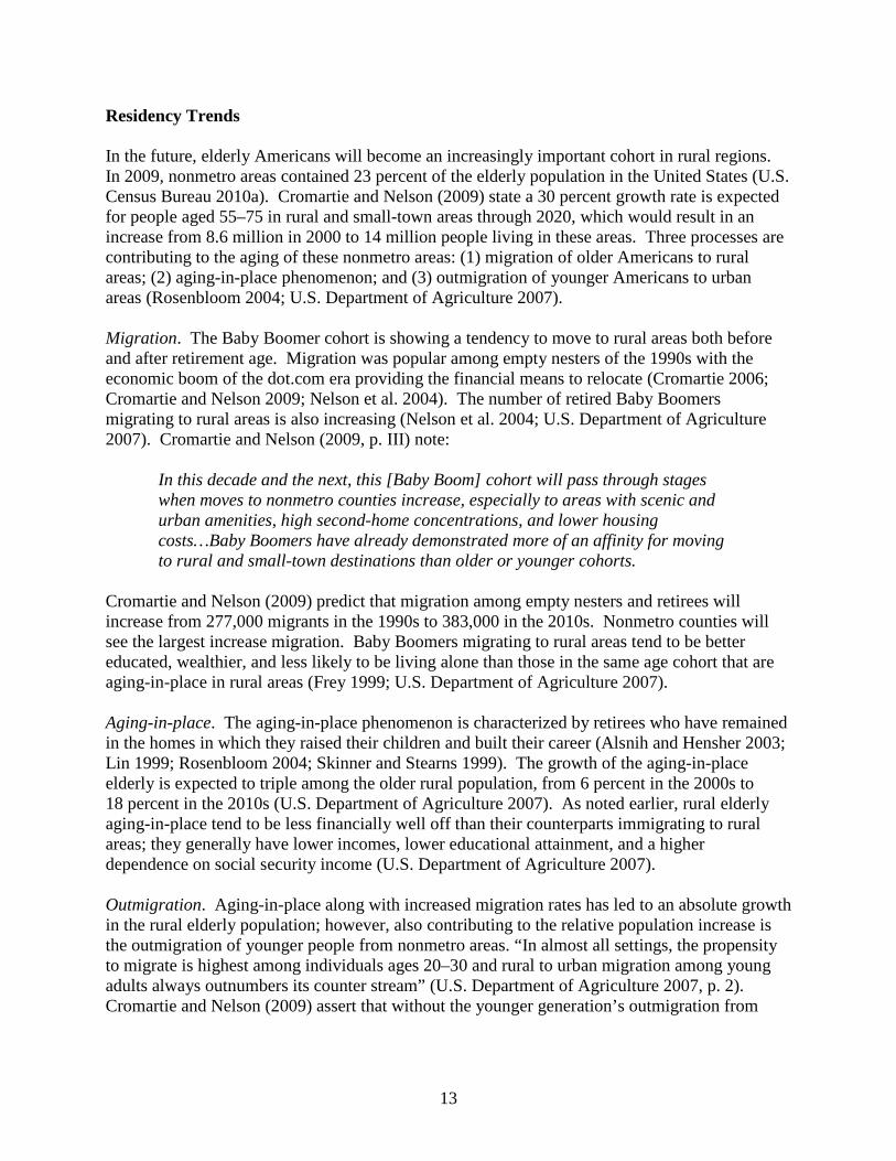
(Figure 2), the percentage of those aged 65–75 has decreased, while the percentage of people over the age of 80 has increased relative to the entire elderly cohort (Figure 3). Texans over the age of 85 have grown from 7 percent of the elderly population in 1970 to 13 percent in 2009 (Figure 3).
Figure 2. Distribution of Texas Elderly by Age Grouping
Figure 3. Percentage of Each Age Group among the Elderly Cohort
0.000.250.500.751.001.251.501.752.002.252.502.75
Popu
latio
n (M
illio
ns)
Year
ages 65-69 ages 70-74 ages 75-79 ages 80-84 ages 85 and up
0%10%20%30%40%50%60%70%80%90%
100%
Perc
enta
ge o
f Eld
erly
Coh
ort
Year
ages 65-69 ages 70-74 ages 75-79 ages 80-84 ages 85 and up
13
Residency Trends In the future, elderly Americans will become an increasingly important cohort in rural regions. In 2009, nonmetro areas contained 23 percent of the elderly population in the United States (U.S. Census Bureau 2010a). Cromartie and Nelson (2009) state a 30 percent growth rate is expected for people aged 55–75 in rural and small-town areas through 2020, which would result in an increase from 8.6 million in 2000 to 14 million people living in these areas. Three processes are contributing to the aging of these nonmetro areas: (1) migration of older Americans to rural areas; (2) aging-in-place phenomenon; and (3) outmigration of younger Americans to urban areas (Rosenbloom 2004; U.S. Department of Agriculture 2007). Migration. The Baby Boomer cohort is showing a tendency to move to rural areas both before and after retirement age. Migration was popular among empty nesters of the 1990s with the economic boom of the dot.com era providing the financial means to relocate (Cromartie 2006; Cromartie and Nelson 2009; Nelson et al. 2004). The number of retired Baby Boomers migrating to rural areas is also increasing (Nelson et al. 2004; U.S. Department of Agriculture 2007). Cromartie and Nelson (2009, p. III) note:
In this decade and the next, this [Baby Boom] cohort will pass through stages when moves to nonmetro counties increase, especially to areas with scenic and urban amenities, high second-home concentrations, and lower housing costs…Baby Boomers have already demonstrated more of an affinity for moving to rural and small-town destinations than older or younger cohorts.
Cromartie and Nelson (2009) predict that migration among empty nesters and retirees will increase from 277,000 migrants in the 1990s to 383,000 in the 2010s. Nonmetro counties will see the largest increase migration. Baby Boomers migrating to rural areas tend to be better educated, wealthier, and less likely to be living alone than those in the same age cohort that are aging-in-place in rural areas (Frey 1999; U.S. Department of Agriculture 2007). Aging-in-place. The aging-in-place phenomenon is characterized by retirees who have remained in the homes in which they raised their children and built their career (Alsnih and Hensher 2003; Lin 1999; Rosenbloom 2004; Skinner and Stearns 1999). The growth of the aging-in-place elderly is expected to triple among the older rural population, from 6 percent in the 2000s to 18 percent in the 2010s (U.S. Department of Agriculture 2007). As noted earlier, rural elderly aging-in-place tend to be less financially well off than their counterparts immigrating to rural areas; they generally have lower incomes, lower educational attainment, and a higher dependence on social security income (U.S. Department of Agriculture 2007).
Outmigration. Aging-in-place along with increased migration rates has led to an absolute growth in the rural elderly population; however, also contributing to the relative population increase is the outmigration of younger people from nonmetro areas. “In almost all settings, the propensity to migrate is highest among individuals ages 20–30 and rural to urban migration among young adults always outnumbers its counter stream” (U.S. Department of Agriculture 2007, p. 2). Cromartie and Nelson (2009) assert that without the younger generation’s outmigration from
14
rural areas, the rate of percentage growth in these areas between 2010 and 2020 for those aged 65 and older would be cut nearly in half. MOBILITY AND THE ELDERLY Numerous factors contribute to the quality of life for both the elderly and nonelderly. Acknowledging the importance of all these issues, the following literature review concentrates on one factor, transportation issues that affect mobility. Further, this review only tangentially addresses the important issue of medical transportation for the elderly. This is not to down play the importance of this issue, but many studies on medical transportation exist. For a discussion of the issues related to medical transportation see Arcury et al. (2005), Mattson (2010), Wallace et al. (2006), and Wallace et al. (2005). Mobility is defined as a person’s ability to travel (Robson 1982) or the freedom, independence, and convenience of movement for non-medical activities (Burns 1999). As suggested in the demographic section, mobility of the growing elderly population will become an increasingly important public policy issue. By far, the majority of previous studies have addressed elderly mobility from a sociological perspective using surveys that are usually limited to responses from elderly individuals. Few if any, studies have addressed the problem from the perspective of the general public’s opinions of or willingness-to-pay for services that enhance the mobility of the elderly. Burns (1999) states that well-being is dependent upon the fulfillment of one’s needs. Mobility and the availability of transportation contribute to this fulfillment by helping one meet medical, social, and personal needs. In general, because the rural elderly are more isolated and usually live at a greater distance from medical and other services than their urban counterparts, transportation options are central to meeting the requirements of the rural elderly (Glasgow and Blakely 2000; Revis 1971). Grant and Rice (1983) report that 18.5 percent of the rural elderly have a serious problem with transportation to almost all destinations. Within the American lifestyle, there is no question of the importance of transportation to the quality of life of people of all ages. Transportation services may become limited as people age. Car Usage by the Elderly Rosenbloom (2004, p. 4) states, “Regardless of where they live, most older people are extremely dependent on the private car.” Because the private automobile has become the most popular form of transportation in today’s culture, today’s elderly have become accustomed to the uses and convenience of a car; pre-retirement and during retirement the car remains the most efficient manner to fulfill most every day mobility needs (Alsnih and Hensher 2003). In rural households, automobile ownership is more prevalent than among urban households because of the relatively longer distances to travel to services and lack of alternative transportation options (Brown 2008; Gombeski and Smolensky 1980; McGhee 1983). Licensing rates are expected to grow for the elderly. In 1997, more than 95 percent of men and 80 percent of women over the age of 65 were licensed to drive (Rosenbloom 2004). As Baby Boomers age, the gap between men and women licensed drivers most likely will narrow.
15
Evidence of this potential shrinking gap is seen in that 94 percent of women aged 45–49 were licensed to drive in 2009 (Rosenbloom 2004). Concerns Associated with Driving. Driving, although the most convenient mode of transportation has its own set of benefits and concerns. The most obvious benefit is the freedom of mobility associated with driving oneself. This freedom motivates the elderly to continue driving even when driving becomes a difficult task (Burns 1999). Elderly drivers note that as they age they suffer from handicaps that cause them to have trouble driving (Glasgow and Blakely 2000). To compensate for age related disabilities, the elderly may limit their driving behavior. Because of poorer night vision and problems with headlight glare, many elderly drivers avoid driving at nighttime or on poorly lit roads (British Automobile Association 1988; Rosenbloom 2004 and 2009). In addition to night driving, rush hours, turning across traffic, city centers, highways, long trips, bad weather, and unfamiliar routes are cited as driving situations the elderly frequently avoid (British Automobile Association 1988; Burns 1999). Further, safety is a concern for older drivers. The elderly are more likely to experience a crash per trip or mile driven and are more likely to be at fault, killed, or injured in a multicar crash than younger aged drivers (Dellinger et al. 2002). For example in 1997, the fatality rate for drivers 85 and over was nine times as high as the rate for drivers 25 through 69 years old (National Highway Traffic Administration 1999). In 2000, people who were 65 and older had the second highest death rate from motor vehicle accidents (He et al. 2005). Although more elderly are licensed to drive and dependent on their personal vehicle than previous generations, they may eventually have to stop driving. Some stop because of family or society pressures, but others cite age-related disabilities and health problems as reasons they stopped driving (Glasgow and Blakely 2000). Because people are living longer, an increasing percentage of the elderly will face disabilities (He et al. 2005; Rosenbloom 2004). In 1997, almost 35 percent of individuals over age 80 reported that their disabilities were severe enough to require assistance (Rosenbloom 2004). Furthermore, because of fixed and limited incomes, the elderly may not be able to afford the ownership costs of automobiles, payments, insurance, and maintenance, even if disabilities are not an issue (Gombeski and Smolensky 1980). The cost of ownership may be a particular problem for older women and minorities because these groups have higher poverty rates than older Anglo males (Rosenbloom 2004). Alternative Transportation Options At some point in their life, disabilities, monetary issues, or other reasons may cause an older person to depend on services other than their personal automobile for mobility. Those living in rural communities are often at a greater disadvantage than older urban residents because non-metropolitan areas usually have more limited public transportation and/or private taxi services than metropolitan areas. Further as previously noted, rural persons generally live relatively greater distances from services and amenities in their community than urbanites (Talbot 1985). Options most frequently used by the elderly to overcome no longer being able to drive are: rides
16
from family and neighbors, walking, and public transportation (Glasgow and Blakely 2000; Gombeski and Smolensky 1980; Rosenbloom 2004 and 2009). Rides from Family and Neighbors. As age increases, there is a tendency to become more dependent on others for transportation (Gombeski and Smolensky 1980). Some elderly do not ask for rides because they do not want to burden their friends or family with driving them to do personal errands. As such, their mobility needs are not always fulfilled; this is especially true for non-medical trips (Glasgow and Blakely 2000).
Older individuals who do not drive are often reliant on friends who are of similar age. Two reasons, often cited in the literature, for relying on older friends are that family members do not live nearby or they are limited by work schedules (Glasgow and Blakely 2000). As noted earlier, children are less likely to live near their rural elderly parents because of the popularity of outmigration from rural areas among younger people. Second, even if living in the area, younger people may not be able to help with daily errands because of work schedules. Because of these reasons, asking neighbors or friends of the same age for rides is often easier than asking younger family members (Glasgow and Blakely 2000). If the friend/neighbor driver is also elderly, asking for rides can often pose the same risks as if the original older person was driving. Furthermore, at some point the older friend may lose the ability to drive. If one or more people depend on this person for transportation, not being able to drive reduces the mobility of several elderly individuals (Rosenbloom 1993). Walking. Walking, behind car travel, is the second most popular travel mode for older people in the U.S. (Rosenbloom 2004). Urban and rural individuals over the age of 65 walk to a trip destination about 9 percent of the time, this percentage increases to one out of every four trips if they do not drive (Sweeney 2004). Complaints noted by older pedestrians, include the lack of sidewalks or system of connected sidewalks, upkeep, obstruction problems, and safety concerns (Rosenbloom 2009, Rosenbloom and Herbel 2009). These complaints are undoubtedly compounded in rural areas where activity locations are often too distant to feasibly reach by walking (Glasgow and Blakely 2000).
Private and Public Transportation Alternatives. Transportation alternatives, such as private taxi services, public buses, and Americans with Disabilities Act (ADA) paratransit services are available to the elderly. These forms are not often used among older Americans (Kim and Ulfarsson 2004; Rosenbloom 2004 and 2009; Glasgow and Blakely 2000). In fact, the use of these modes of transportation by the elderly has been decreasing. In 1995, the elderly made 2.2 percent of all trips by transit; this percentage has fallen by almost 50 percent between 1995 and 2001 (Pucher and Renee 2003). Although the reasons for this drop are not explicitly explained, implicit reasons for the unpopularity of these transportation alternatives described in the literature are outlined below.
Taxi Use. Private taxi services are often nonexistent in rural areas because riders and destinations are often so widely dispersed that the cost of operating these services is high (Grant and Rice 1983; McGhee 1983). Even if available, elderly individuals note that private transportation services are often too expensive for them to use (Glasgow and Blakely 2000). Because private transit services are not available, the option left for rural individuals is to use
17
public transit services; in rural areas these services are also often limited (Glasgow and Blakely 2000; Grant and Rice 1983; Mattson 2011).
Rural Public Transportation. Rural public transportation is typically demand response transit and requires advance reservation, usually at least 24-hours in advance. The level of service depends on available resources. The rural American transit system is not adequate compared to the services provided in urban areas (Brown and Stommes 2004; Stommes and Brown 2002). In 2009, 77 percent of rural American counties recorded some type of public transportation in their community (Transit Cooperative Research Program 2009b). Few of these transit systems are found in the most rural and isolated areas; the majority of these systems are county-based, followed by the multi-county level, and then by the municipal level (Transit Cooperative Research Program 2009a). Rural public transportation access and options have come under scrutiny over the past 30 years, especially in poorer nonmetro communities that have large concentrations of the elderly and disabled (Brown 2008). Although strides have been made to improve rural public transportation, rising costs and limited funding continue to hinder the growth of these programs (Transit Cooperative Research Program 2009b). Studies indicate that both transportation professionals and the elderly feel the public transportation service does not adequately assist older rural residents (Brown and Stommes 2004; Foster et al. 1996).
ADA Complementary Paratransit Services. ADA paratransit is a required complementary service for people with disabilities in areas where there is fixed route transit.3 The majority of rural public transportation options do not include fixed routes; ADA paratransit services are often not available in rural areas (Rosenbloom 2004). Services provided by ADA paratransit may fail to assist elderly citizens who are unable to drive or cannot use conventional public transportation (Rosenbloom 2004 and 2009).
Additionally, even if access to ADA paratransit services is available to an elderly individual, he/she may not be qualified to use them. Rosenbloom (2009, p 34) states:
Indeed, the vast number of older people in the United States do not and probably will not live in or travel in neighborhoods with ADA paratransit service, and, even if they do live or travel in such corridors, they are unlikely to qualify for those services for most of their lives after they reach age 65.
Eligibility for ADA services is based on disability and not age; therefore, having minor age related handicaps or being unable to drive does not necessarily qualify an individual for ADA paratransit. For example, in 2009, 42 percent of elderly people with at least one disability were not eligible for these services because their impairments were not serious enough to meet ADA eligibility requirements (Rosenbloom 2009). Public Transportation and Travel Independence. Even if an elderly individual has access to public transit (public bus, ADA paratransit, etc.), these services may not provide the means to be an independent traveler. Elderly individuals indicate that public transportation schedules do not allow them flexibility when making trip plans, because they often must schedule a trip in 3 Fixed route transit refers to transit that operates along a specific defined route. Passengers board and exit at designated stops along the route according to a preset schedule.
18
advance and are confined to time and route limitations of the transit schedules (Foster et al. 1996; Glasgow and Blakely 2000; Mattson 2011; Rosenbloom 2004 and 2009). Rural transit systems in particular often stop at the county line. By the way the transportation system is structured, an individual traveling cannot expect to connect seamlessly to another county-based transit system or intercity bus service (Stommes and Brown 2002). Even non-profit community groups that provide client transit services are not always flexible. They often limit travel to destinations deemed essential, such as medical appointments, even though these trips make up no more than 5 percent of the total trips that older people take (Rosenbloom 2009). Public Transportation in Rural Texas Public transportation in Texas is provided by 38 rural transit districts, 30 urban transit systems, and nine metropolitan transit authorities or departments. A rural transit district serves non-urbanized areas with populations of less than 50,000 and is required by Texas statute to provide and coordinate rural public transportation in its rural territory. In 2010, elderly Texans represented an estimated 34 percent of the population in rural transit districts as compared to 24 percent of the total Texas population (Eschbach et al. 2010). The elderly population is expected to increase in 30 of the 38 rural transit districts, which suggests that demand for rural public transportation will increase (Eschbach et al. 2010). Because of this increasing demand, current transportation services may need to be restructured to reflect the preferences of this population. The current national and state level budget crunches have caused per capita investment in Texas transportation services to decline (Eschbach et al. 2010). Without new funding there most likely will be a reallocation of funds to assist transit in areas with the largest total population growth (metropolitan areas and counties along the Texas-Mexico border), which means there may not be sufficient funds for new or restructured transit services in rural areas (Eschbach et al. 2010). Quality of Life Implications Although there are advantages associated with living in a rural area, the well-being of older rural residents may suffer from several disadvantages unique to these areas. The variety of and access to health care and other personal services is more limited in rural areas; attracting doctors, nurses, and other service professionals is difficult where per capita costs are higher, the population is sparse, and the area is more isolated (Mattson 2011; U.S. Department of Agriculture 2007). Previous literature indicates the elderly receive a substantial amount of support from their children and relatives to overcome these barriers (Grant and Rice 1983; Gombeski and Smolensky 1980; McGhee 1983). This support may not be available as younger generations become more career oriented, move farther away from their aging parents, and family size decreases (Glasgow and Blakely 2000; Putnam 1995; U.S. Department of Agriculture 2007). When an elderly individual is no longer able to drive, without support, these issues can be exaggerated and the individual may experience a decrease in their quality of life. Inadequate transportation arrangements have been cited as a significant contributor to lower life satisfaction, morale, and health. Glasgow and Blakely (2000) find that loneliness was a cited problem among nonmetropolitan older residents. A participant in Glasgow and Blakely (2000, p. 113) is quoted as saying:
19
Don’t you think the biggest share of the senior citizens’ problems is loneliness? You know. They don’t have families. They get older and older and older each day. They get so confined to their homes. Whereas, if they got a bus they know is there, they are going to help them on the bus and sit down, and off the bus very safely. There would be more people who would go out.
This loneliness and lack of participation in the community is detrimental to the emotional and physical health of older individuals (Glasgow and Blakely 2000). Inadequate transportation options also reduce older adults' ability to participate in the economy. Non-drivers who are 65 and over make less than half as many shopping trips and trips to restaurants and other places to eat as other drivers do (Bailey 2004). Bailey (2004) concludes that elderly who live in the West South Central states of the U.S. (this area includes Texas) experience a high amount of isolation because of the limited transportation options provided in this area. With the percentage of the elderly rural population growing and the younger rural population diminishing, the elderly are left to depend more on themselves, people of the same age, their community, and government services for their well-being (Alsnih and Hensher 2003; Gombeski and Smolensky 1980; Grant and Rice 1983; Kim and Ulfarsson 2004; McGhee 1983; Rosenbloom 2004 and 2009). Within the American lifestyle, there is no question of the importance of transportation to the quality of life of people of all ages. Transportation services may become limited as people age. These statements are not only true for Americans, but elderly mobility is a worldwide issue (Dejoux et al. 2010; van den Berg et al. 2011; Buehler and Nobis 2010; Ahern and Hine 2012).
CHAPTER 3. METHODOLOGY AND SURVEY DESIGN To achieve the study’s research objectives, a choice survey was created and distributed to Texas A&M University undergraduate students and residents of Atascosa, Polk, and Parker Counties, Texas. The choice survey format provides a tool to obtain economic willingness-to-pay for various transportation options. By surveying both students and county residents, comparisons between opinions of different age/socio-demographic groups can be made. The random utility model provides the basis for econometric models that will be estimated using conditional and mixed logit estimation. QUESTIONNAIRE DESIGN Two similar questionnaires are created, one for the student sample, and the other for the county resident sample. Both questionnaires contained similar questions that were based on previous surveys, the literature, and expert opinions. Two focus groups were held to refine the student survey instrument. An additional focus group and professional editor from the Texas Transportation Institute provided comments on the county resident questionnaire. Before distribution, approval for the study was obtained by the Texas A&M University Institutional Review Board. Final survey instruments used in the student and county resident surveys are in Appendices A and B.
20
Focus Groups – Students Two focus groups of students enrolled at Texas A&M University-College Station were conducted. The first focus group met on April 4, 2011, at 1PM, whereas, the second met on April 11, 2011, at 10AM. Participants in the first focus group consisted of six graduate students; four were enrolled in the Department of Agricultural Economics, one in the Department of Oceanography, and one the Department of Computer Science. This focus group consisted of three males and three females. Their hometowns were located in Texas, Kansas, California, Canada, and Morocco. Five of the participants’ homes were located within the city limits and one was located outside the city limits on a farm. The focus group organization was a free flowing but directed discussion. In particular, the discussion was directed toward three main topics: questionnaire length, question wording and formatting, and factors that would influence their decisions. The first focus group unanimously agreed that the questionnaire was too lengthy. They commented that some questions and sections were too wordy, which made respondents lose focus. It took the focus group members between 10 and 15 minutes to complete the questionnaire. Further, the group noted some questions concerning the respondents’ hometown (i.e., the distance the respondent lives from his/her parents) may be hard to answer given the respondent’s parent’s marital status. Questions to identify the respondents’ familiarity with elderly transportation issues were worded too similarly; therefore, making them difficult to answer. The largest fee that anyone in the focus group would be willing to pay for any of the transportation options was $30. The majority of participants thought that the days and hours the transportation option would be in service were important attributes. The actual days and hours (i.e., seven days a week from 8AM to 5PM) of operation would be more important in making a decision than just the number of days and hours (i.e., three days a week for 8 hours a day). Some participants believed that although more hours and days were better, individuals could adjust their schedules to limited days and hours in operation. The range of service area was also important to the focus group, but they were confused on how to interpret the size of the service area. The participants thought a fare discount for senior citizens was important, but they thought it was the least important factor in making a decision. Given an original fare of $2.00, the participants thought that any discount would be inconsequential given the original fare was already low. Overall, the participants of the first focus group preferred transportation attributes which were the most flexible and accommodating of senior citizens. They had trouble interpreting the levels of transportation attributes.
After revising the questionnaire, a second focus group was conducted. This group consisted of four graduate students enrolled in the Department of Statistics and two undergraduate students enrolled in the Department of Mathematics and Biochemistry/Genetics. One of the student’s home towns was located in North Carolina, whereas, the other five were located in Texas. Two of the student’s homes were located inside their hometown’s city limits; the other four were located on the boundary of the city limits. The organization was similar to the first focus group, focusing on the same topics.
Although the length of the questionnaire was still an issue with this focus group, this version took the participants considerably less time to complete; all finished within eight to 10 minutes.
21
Most of the previous issues with the original questionnaire seemed to be addressed. The focus group had trouble when ranking their familiarity of their hometown’s public transportation options. Most did not know if any public transit existed in their hometown, hence answering “not at all familiar” was not necessarily a true observation. It was suggested to add a question addressing whether or not the respondent is aware of transportation options in their hometown. The questions used to identify the respondents’ familiarity with elderly transportation issues were again difficult to answer. One of the participants noted that it was not clear how to include deceased family members when answering the question. Also, it was difficult to distinguish between a “do not know” and a “no” answer. This focus group’s opinions about the transportation attributes were similar to the first focus group. Flexible days and hours of operation were extremely important. The range of service was important; however, further clarification of the levels of this attribute would be preferred. This focus group had mixed opinions on the importance of the fare discount. Those who supported or were against a discount had very strong opinions in either case. Overall, this attribute was least important in the focus group’s decision making process.
Focus Group – County Residents After revising the questionnaire and adding county specific questions, a focus group of Atascosa County residents was conducted on July 21 at 6PM in the Pleasanton, Texas City Hall. This focus group included seven people who resided in Atascosa County. Six lived in Pleasanton and one lived in the town of Jourdanton. The focus group included three males and four females. Format of the issues presented to the group followed a similar procedure as the previous two focus groups. The main issue presented to the focus group was to consider the audience of people who would be filling out the questionnaire; they suggested some clarification of the questions and introductions would be necessary. For example, in answering a question which mentioned the respondent’s dependents, one of the participants was confused as to who to consider as “dependents.” He considered his wife a dependent; as such he was not clear how to answer the question. The group suggested changing the phrase from “children or dependents” to “children or dependents, excluding your spouse.” One of the participants mentioned that she had more than one mailing address within the county. She suggested that we use the phrase “primary mailing address” to clarify the question. All participants were unsure of how to answer whether or not they knew about the Alamo Regional Transit (ART) options in the county. Most had seen ART vehicles but had no idea what they did or who could use them. They could not answer yes to the question because it asked if the respondent was, “Aware of the public transportation options provided by ART.” The objective of that question is to determine if the respondent knew of ART, then a following series of questions were included to give an idea if the respondent knew the details about ART’s public transit options. The focus group agreed that by leaving ‘options’ out of the first question it would be easier to respond correctly. Other suggestions from the focus group included: shorten the content included in the introduction to the choice questions; further clarify the hypothetical nature of the survey; and highlight the statement “Please consider each of the following six scenarios independently” so there is no confusion on how to fill out the choice questions. Participants of this focus group felt that all transportation attributes were important in their decision making process. Although the definitions of the attributes were lengthy, each
22
respondent felt they clearly understood the levels of each attribute. Again, the questionnaire was revised based on the focus groups comments.
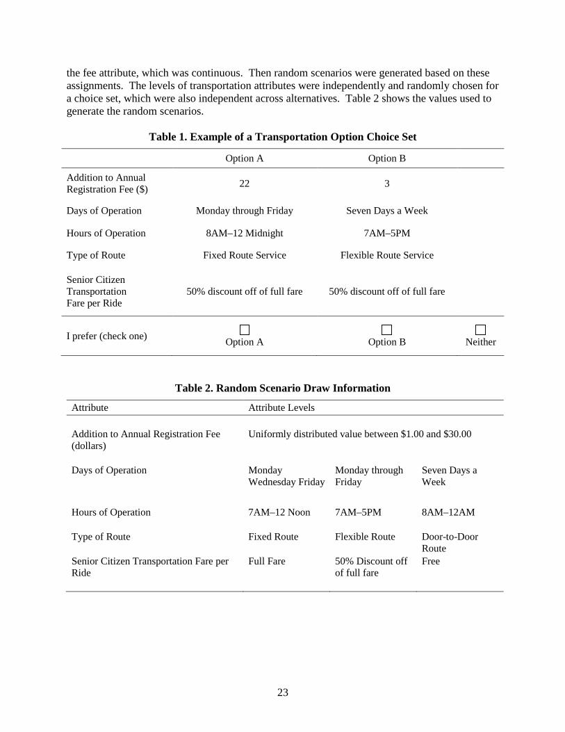
SURVEY QUESTIONNAIRE DESIGN The questionnaire contained a series of questions to provide background information on the respondent. These questions included common demographic inquiries like age, sex, race, and income. Some demographic questions were specific to the student or county resident questionnaires. To determine income, for instance, county residents were directly asked for their before-tax income. Students were asked what percentage of their funding for school came from which various sources (parents, self, scholarship, military, etc.). County residents were also asked how far away each of their dependents lived from the resident’s home. All respondents were asked questions about their knowledge of and opinions about local public transit opportunities. Finally, respondents were asked to provide their subjective probability that they would live to be over 75, live in rural community, and need assistance with transportation. These inquiries into respondents’ subjective probabilities were designed similarly to questions asked by the Institute for Social Research (2010). Choice Scenario Design. One critical part of the survey is the choice experiment design. The Choice Experiment, which is in the family of choice modeling approaches, provides a useful methodology to obtain welfare consistent estimation for evaluating the monetary value of different attributes (Hanley et al. 2001). In this type of study, respondents are presented with two or more alternatives, where each differs only in terms of attribute levels and are asked to choose the option most preferred. Within the choice set, the respondent is also presented with the option to do nothing or a baseline alternative referring to the status quo. This baseline is necessary to interpret the results in standard welfare economic terms (Hanley et al. 2001). By including price or cost as one of the attributes of the good, willingness-to-pay can be indirectly estimated from the responses (Hanley et al. 2001). The respondents were given six choice scenarios; in each scenario they were asked to choose between two public transportation options that would be funded by this fee (Option A and Option B) or to choose neither of the two options (Neither). In each of the scenarios, different levels of each transportation attribute were presented to the respondent. The options in a scenario contained the same attributes but differed in the levels of the attributes. In the questionnaire, respondents were informed that to fund public transportation options that benefit rural elderly Texans, a fee will be added to the current costs of registering their vehicle. This fee amount constituted one attribute in each option. The attributes that characterize each transportation option in one choice scenario are: (1) the addition to yearly registration fee; (2) days of operation; (3) hours of operation; (4) type of route; and (5) fare discount given to senior citizens. Table 1 shows an example of a scenario. The attributes and their levels are based upon previous surveys in the literature, although these surveys did not employ a choice survey format (Foster et al. 1996; Glasgow and Blakely 2000; Gombeski and Smolensky 1980; Grant and Rice 1983). The focus group discussions, as well as transportation experts, were helpful in designing the level of transportation attributes. To assign levels to a particular choice set, each level of an attribute was assigned a distinct number, except
23
the fee attribute, which was continuous. Then random scenarios were generated based on these assignments. The levels of transportation attributes were independently and randomly chosen for a choice set, which were also independent across alternatives. Table 2 shows the values used to generate the random scenarios.
Table 1. Example of a Transportation Option Choice Set
Option A Option B
Addition to Annual Registration Fee ($) 22 3
Days of Operation Monday through Friday Seven Days a Week
Hours of Operation 8AM–12 Midnight 7AM–5PM
Type of Route Fixed Route Service Flexible Route Service
Senior Citizen Transportation Fare per Ride
50% discount off of full fare 50% discount off of full fare
I prefer (check one) Option A
Option B
Neither
Table 2. Random Scenario Draw Information
Attribute Attribute Levels Addition to Annual Registration Fee (dollars)
Uniformly distributed value between $1.00 and $30.00
Days of Operation Monday Wednesday Friday
Monday through Friday
Seven Days a Week
Hours of Operation 7AM–12 Noon
7AM–5PM 8AM–12AM
Type of Route Fixed Route Flexible Route
Door-to-Door Route
Senior Citizen Transportation Fare per Ride
Full Fare 50% Discount off of full fare
Free
24
DATA COLLECTION The student survey was distributed to 507 students attending Texas A&M University. This sample of students was taken from selected classes taught at Texas A&M University-College Station within the College of Agriculture and Life Sciences and Mays Business School. The surveys were distributed in April and May 2011. A second student survey was distributed to students in early 2012. A second questionnaire was distributed by U.S. mail with a (postage paid) return envelope to 3,200 residents equally divided between Atascosa and Polk counties between the dates of September 15 and November 1, 2011. Atascosa County is located in south Texas near San Antonio, whereas, Polk County is located in the Piney Woods region of east Texas. The 2010 population of Atascosa County was 44,911 with the elderly population making up 11 percent of the total population (U.S. Census Bureau 2010b). Polk County’s population of 45,413 has a higher percentage of elderly at 20 percent (U.S. Census Bureau 2010c). Both counties are among the Texas rural counties with the fastest growing elderly populations. From 2000–2009, the elderly population grew by 25 percent and 20 percent in Polk and Atascosa Counties, respectively (U.S. Census Bureau 2000b, 2000c, 2010b, 2010c, 2010d, and 2010e). Atascosa and Polk County are served by rural public transportation systems, Alamo Regional Transit, and The Brazos Transit District. Names and addresses of residents were obtained through an open records request of the Polk and Atascosa County Appraisal District offices. The county questionnaire was distributed by mail based on Dillman’s (1991) total design survey method. This approach involves three mailings. The first mailing made on September 15, included the questionnaire and a letter informing the recipient of the issue and inviting them to participate. On September 25, a reminder postcard was sent to those who had not responded to the first mailing. Finally, on October 5, the survey instrument was mailed to those people who had not responded. In addition, the local newspapers in Atascosa (The Pleasanton Express) and Polk (The Polk County Enterprise) Counties each printed a news story, around the 15th of October, describing the survey and reminding people to participate in the survey. Because the results of the Atascosa and Polk County surveys were similar and because the research team had more remaining project resources for surveys than anticipated, due to compiling the mailings in house rather than contracting a mailing service, Parker County in north central Texas was surveyed as well in April and May 2012, following the same process as in previous counties. The results of the Parker County survey are reported in a separate chapter.
THE RANDOM UTILITY MODEL AND MODEL SPECIFICATION The random utility model (RUM) provides the theoretical basis for this study. McFadden (1974, 1978, and 1981) is often noted as a pioneer of discrete choice models in economics; his papers expand on the properties that link discrete choice to utility maximization. The RUM has been extensively used by previous studies in a variety of situations including: non-market valuations, health valuations, and situations involving choice models (Bockstael et al. 1984; Craig and Busschbach 2009; Horowitz 1991; Kataria et al. 2012; Lee and Mjelde 2007; Middleton 1991;

25
Parsons and Kealy 1992; Rubey and Lupi 1997; Scarpa et al. 2009). The strength of this model is its ability to describe a decision maker’s choice among a set of mutually exclusive alternatives in a statistically estimated form. The RUM is based on the notion that an individual derives more utility from the chosen alternative than from those alternatives not chosen. The indirect utility function, 𝑈𝑖𝑛, forms the basis for the RUM framework. In this framework, the utility that individual i receives from choosing alternative n can be obtained from a set of explanatory variables 𝑧𝑖𝑛 and an unknown random component 𝜀𝑖𝑛. We denote 𝑧𝑖𝑛 = [𝑥𝑖𝑛,𝑤𝑖] where 𝑤𝑖 represents individual characteristics that vary across individuals but are the same for all alternatives presented to the same individual; and 𝑥𝑖𝑛 includes attributes of alternatives that vary across alternatives and individuals. Given this information, the linear RUM for individual i choosing alternative n in a choice scenario t is (Greene 2003):
(1) 𝑈𝑖𝑛𝑡(𝑥𝑖𝑛𝑡,𝑤𝑖) = 𝑧𝑖𝑛𝑡′ 𝛽 + 𝜀𝑖𝑛𝑡
where 𝑈𝑖𝑛𝑡 is the indirect utility function, β is a vector of parameters to be estimated, and the error term is denoted as 𝜀𝑖𝑛𝑡. The RUM assumes utility maximization such that decision maker i will choose alternative n over m in the choice scenario t, if and only if:
(2) 𝑈𝑖𝑛𝑡(𝑥𝑖𝑛𝑡,𝑤𝑖) > 𝑈𝑖𝑚𝑡(𝑥𝑖𝑚𝑡,𝑤𝑖) ∀ 𝑛 ≠ 𝑚.
Assumptions made about the distribution of the disturbance term and whether the coefficients are fixed or varying across individuals in the RUM model lead to the use of various qualitative models to estimate the RUM. Two variants of the logit model, conditional and mixed, are used in this study. The logit family of models is recognized as the essential toolkit for analyzing discrete choices because of their consistency with random utility theory (Hensher and Greene 2003). Conditional Logit Model For a given choice set, t, the probability that respondent i prefers alternative n over m is stated as the probability the utility associated with alternative n exceeds the utility associated with all the other alternatives indexed by m:
(3) 𝑃(𝑈𝑖𝑛𝑡 > 𝑈𝑖𝑚𝑡 ∀ 𝑛 ≠ 𝑚) = 𝑃{(𝑧𝑖𝑛𝑡′ 𝛽 − 𝑧𝑖𝑚𝑡′ 𝛽) > (𝜀𝑖𝑚𝑡 − 𝜀𝑖𝑛𝑡)}. To derive the probability in equation (3), the random errors (𝜀𝑖𝑛𝑡, 𝜀𝑖𝑚𝑡) are assumed to be identically and independently distributed with an extreme-value (Greene 2003):
(4) 𝐹(𝜀𝑖𝑛𝑡) = exp (−𝜀𝑖𝑛𝑡−𝜀𝑖𝑛𝑡)
26
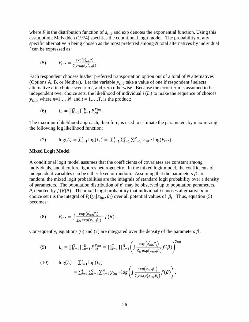
where F is the distribution function of 𝜀𝑖𝑛𝑡 and exp denotes the exponential function. Using this assumption, McFadden (1974) specifies the conditional logit model. The probability of any specific alternative n being chosen as the most preferred among N total alternatives by individual i can be expressed as:
(5) 𝑃𝑖𝑛𝑡 = exp�𝑧𝑖𝑛𝑡′ 𝛽�
∑ exp�𝑧𝑖𝑛𝑡′ 𝛽�𝑁
.
Each respondent chooses his/her preferred transportation option out of a total of N alternatives (Options A, B, or Neither). Let the variable 𝑦𝑖𝑛𝑡 take a value of one if respondent i selects alternative n in choice scenario t, and zero otherwise. Because the error term is assumed to be independent over choice sets, the likelihood of individual i (Li) to make the sequence of choices 𝑦𝑖𝑛𝑡, where n=1,…,N and t = 1,…,T, is the product:
(6) 𝐿𝑖 = ∏ ∏ 𝑃𝑖𝑛𝑡𝑦𝑖𝑛𝑡N
n=1Tt=1 .
The maximum likelihood approach, therefore, is used to estimate the parameters by maximizing the following log likelihood function:
(7) log(𝐿) = ∑ log (𝐿𝑖)𝐼𝑖=1 = ∑ ∑ ∑ 𝑦𝑖𝑛𝑡 ∙ log (𝑃𝑖𝑛𝑡)𝑁
𝑛=1𝑇𝑡=1
𝐼𝑖=1 .
Mixed Logit Model A conditional logit model assumes that the coefficients of covariates are constant among individuals, and therefore, ignores heterogeneity. In the mixed logit model, the coefficients of independent variables can be either fixed or random. Assuming that the parameters 𝛽 are random, the mixed logit probabilities are the integrals of standard logit probability over a density of parameters. The population distribution of 𝛽𝑖 may be observed up to population parameters, θ, denoted by 𝑓(𝛽|𝜃). The mixed logit probability that individual i chooses alternative n in choice set t is the integral of 𝑃𝑖(𝑦𝑖|𝑧𝑖𝑛𝑡,𝛽𝑖) over all potential values of 𝛽𝑖. Thus, equation (5) becomes:
(8) 𝑃𝑖𝑛𝑡 = ∫exp(𝑧𝑖𝑛𝑡′ 𝛽𝑖)
∑ exp(𝑧𝑖𝑛𝑡′ 𝛽𝑖)𝑁∙ 𝑓(𝛽).
Consequently, equations (6) and (7) are integrated over the density of the parameters 𝛽:
(9) 𝐿𝑖 = ∏ ∏ 𝑃𝑖𝑛𝑡𝑦𝑖𝑛𝑡N
n=1Tt=1 = ∏ ∏ �∫
exp�𝑧𝑖𝑛𝑡′ 𝛽𝑖�∑ exp�𝑧𝑖𝑛𝑡′ 𝛽𝑖�𝑁
𝑓(𝛽)�yint
Nn=1
Tt=1
(10) log(𝐿) = ∑ log (𝐿𝑖)𝐼
𝑖=1
= ∑ ∑ ∑ 𝑦𝑖𝑛𝑡 ∙ log �∫𝑒𝑥𝑝�𝑧𝑖𝑛𝑡′ 𝛽𝑖�
∑ 𝑒𝑥𝑝�𝑧𝑖𝑛𝑡′ 𝛽𝑖�𝑁𝑓(𝛽)�𝑁
𝑛=1𝑇𝑡=1
𝐼𝑖=1 .
27
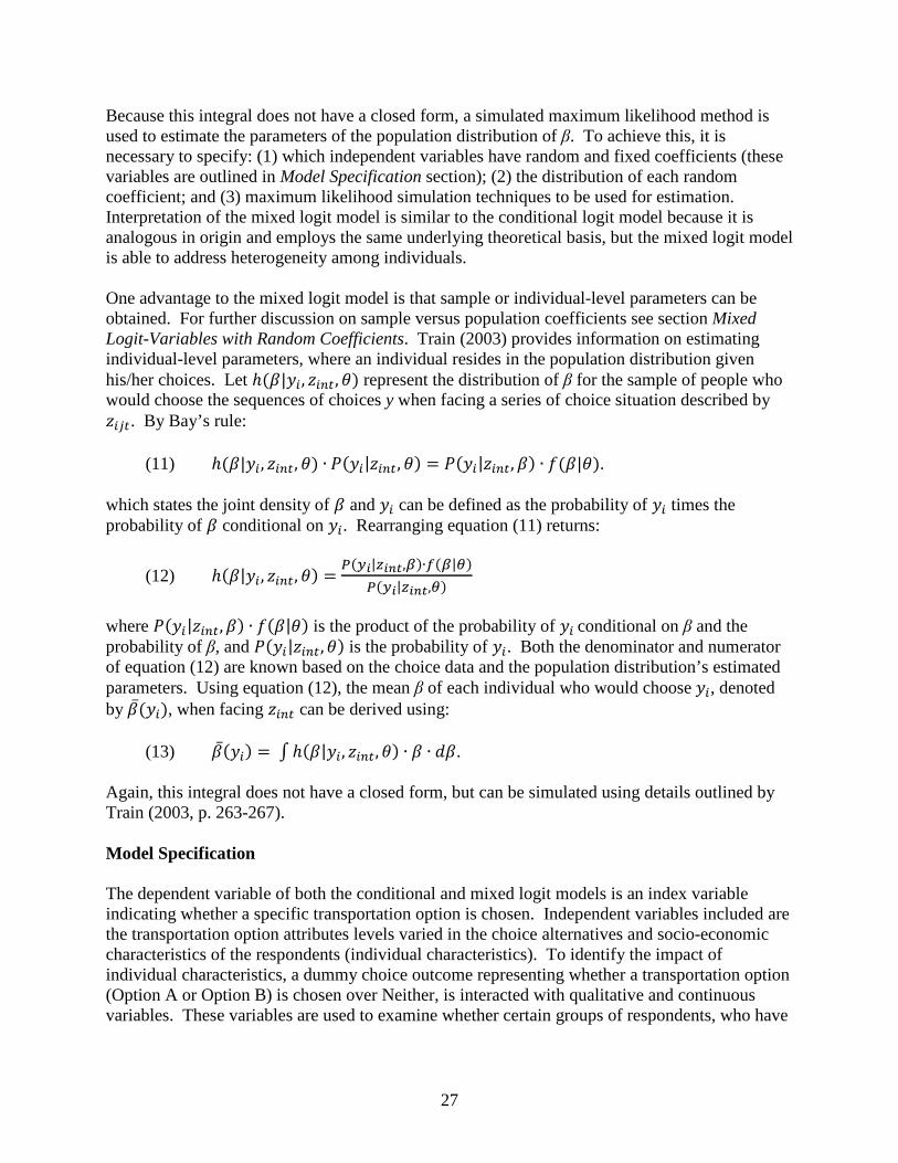
Because this integral does not have a closed form, a simulated maximum likelihood method is used to estimate the parameters of the population distribution of β. To achieve this, it is necessary to specify: (1) which independent variables have random and fixed coefficients (these variables are outlined in Model Specification section); (2) the distribution of each random coefficient; and (3) maximum likelihood simulation techniques to be used for estimation. Interpretation of the mixed logit model is similar to the conditional logit model because it is analogous in origin and employs the same underlying theoretical basis, but the mixed logit model is able to address heterogeneity among individuals. One advantage to the mixed logit model is that sample or individual-level parameters can be obtained. For further discussion on sample versus population coefficients see section Mixed Logit-Variables with Random Coefficients. Train (2003) provides information on estimating individual-level parameters, where an individual resides in the population distribution given his/her choices. Let ℎ(𝛽|𝑦𝑖, 𝑧𝑖𝑛𝑡,𝜃) represent the distribution of β for the sample of people who would choose the sequences of choices y when facing a series of choice situation described by 𝑧𝑖𝑗𝑡. By Bay’s rule:
(11) ℎ(𝛽|𝑦𝑖, 𝑧𝑖𝑛𝑡, 𝜃) ∙ 𝑃(𝑦𝑖|𝑧𝑖𝑛𝑡, 𝜃) = 𝑃(𝑦𝑖|𝑧𝑖𝑛𝑡,𝛽) ∙ 𝑓(𝛽|𝜃). which states the joint density of 𝛽 and 𝑦𝑖 can be defined as the probability of 𝑦𝑖 times the probability of 𝛽 conditional on 𝑦𝑖. Rearranging equation (11) returns:
(12) ℎ(𝛽|𝑦𝑖, 𝑧𝑖𝑛𝑡, 𝜃) = 𝑃(𝑦𝑖|𝑧𝑖𝑛𝑡,𝛽)∙𝑓(𝛽|𝜃)
𝑃(𝑦𝑖|𝑧𝑖𝑛𝑡,𝜃)
where 𝑃(𝑦𝑖|𝑧𝑖𝑛𝑡,𝛽) ∙ 𝑓(𝛽|𝜃) is the product of the probability of 𝑦𝑖 conditional on β and the probability of β, and 𝑃(𝑦𝑖|𝑧𝑖𝑛𝑡,𝜃) is the probability of 𝑦𝑖. Both the denominator and numerator of equation (12) are known based on the choice data and the population distribution’s estimated parameters. Using equation (12), the mean β of each individual who would choose 𝑦𝑖, denoted by �̅�(𝑦𝑖), when facing 𝑧𝑖𝑛𝑡 can be derived using:
(13) �̅�(𝑦𝑖) = ∫ ℎ(𝛽|𝑦𝑖, 𝑧𝑖𝑛𝑡,𝜃) ∙ 𝛽 ∙ 𝑑𝛽. Again, this integral does not have a closed form, but can be simulated using details outlined by Train (2003, p. 263-267). Model Specification The dependent variable of both the conditional and mixed logit models is an index variable indicating whether a specific transportation option is chosen. Independent variables included are the transportation option attributes levels varied in the choice alternatives and socio-economic characteristics of the respondents (individual characteristics). To identify the impact of individual characteristics, a dummy choice outcome representing whether a transportation option (Option A or Option B) is chosen over Neither, is interacted with qualitative and continuous variables. These variables are used to examine whether certain groups of respondents, who have
28
the above stated characteristics, are more or less likely to choose a transportation option over neither. Variables with Fixed Coefficients. All independent variables have fixed coefficients in the conditional logit model. This is not the case in the mixed logit model. As indicated previously the mixed logit model can include variables with both fixed and random coefficients. All individual specific characteristics are assumed to have fixed coefficients in the mixed logit model. Although the coefficient for the additional annual registration fee of a transportation option is likely to be negative but differ in magnitude in the population, the coefficient of the registration fee is assumed to be fixed to simplify the willingness-to-pay calculations (outlined in the section Estimating Preferences and Transportation Option Willingness-to-Pay). Under this assumption the distribution of the willingness-to-pay for each non-fee attribute has the same distribution type as the transportation attribute level’s coefficient. Mixed Logit-Variables with Random Coefficients. The coefficients for all transportation option attribute levels, except vehicle registration fee, are assumed to have random coefficients. As in previous random coefficient model literature, it is necessary to make a distinction between the population and the sample. In this study, five populations are considered: (1) the residents of Atascosa County; (2) the residents of Polk County; (3) the residents of Parker County; (4) in-state students enrolled at Texas A&M University in the spring of 2011; and (5) in-state students enrolled at Texas A&M University in the spring of 2012. Sample refers to the group of Atascosa County residents, Polk County residents, Parker County residents, and Texas A&M University students by year who participated (responded to) in the choice survey. To characterize heterogeneous preferences, distributions must be specified for the random coefficients associated with the various transportation option attributes. Respondents may have different preferences as to which transportation option attributes will best serve their elderly community members. People may prefer fewer days and hours of operation if they believe personal schedules can be altered to match the transportation schedule. Some people may believe a fare discount for senior citizens is necessary, whereas, others may think there should not be price discrimination based on age. It is assumed, therefore, the coefficients of transportation option attribute levels can be either positive or negative. Under this supposition, each of these coefficients is assumed to follow an independent normal distribution with mean and standard deviation to be estimated. Estimating Conditional Logit Transportation Option Willingness-to-Pay. Let the conditional logit estimated coefficients associated with the additional vehicle registration fee be �̂�𝑠 and the transportation attribute k be �̂�𝑘. The mean willingness-to-pay for the various transportation option attributes are then derived using the following formula (Hanley et al. 2001):
(14) WTP = −𝛽�𝑘
𝛽�𝑠 .
29
In the conditional logit model, both �̂�𝑘 and �̂�𝑠 are fixed, therefore, WTP is also a fixed value. The mean WTP represents the amount the population is willing to pay to receive a transportation attribute level over the base level. The standard deviation of the mean WTP derived from the conditional logit model is calculated using a Taylor Series Expansion (Wolter 2007). Let the estimated coefficients �̂�𝑘 = 𝑎 and �̂�𝑠 = 𝑏. The first-order Taylor series expansion at the point (𝑎, 𝑏) is:
(15) 𝑊𝑇𝑃(𝑥,𝑦) ≈ 𝑊𝑇𝑃(𝑎, 𝑏) + (𝑥 − 𝑎) ∙ 𝑊𝑇𝑃𝑥(𝑎, 𝑏) +
(𝑦 − 𝑏) ∙ 𝑊𝑇𝑃𝑦(𝑎, 𝑏) where 𝑊𝑇𝑃(𝑎, 𝑏) is 𝑊𝑇𝑃(𝑥,𝑦) evaluated at the point (𝑎, 𝑏); 𝑊𝑇𝑃𝑥(𝑎, 𝑏) is the partial derivative of 𝑊𝑇𝑃(𝑥,𝑦) with respect to x evaluated at point (𝑎, 𝑏); and 𝑊𝑇𝑃𝑦(𝑎, 𝑏) is the partial derivative of 𝑊𝑇𝑃(𝑥,𝑦) with respect to y evaluated at point (𝑎, 𝑏). The variance of 𝑊𝑇𝑃(𝑎, 𝑏)is:
(16) 𝜎𝑊𝑇𝑃2 = 𝜎𝑥−𝑎2 ∙ (𝑊𝑇𝑃𝑥(𝑎, 𝑏))2 + 𝜎𝑦−𝑏2 ∙ (𝑊𝑇𝑃𝑦(𝑎, 𝑏))2 +
2 ∙ 𝑊𝑇𝑃𝑥(𝑎, 𝑏) ∙ 𝑊𝑇𝑃𝑦(𝑎, 𝑏) ∙ 𝐶𝑜𝑣(𝑥 − 𝑎,𝑦 − 𝑏
= �−1𝑏�2
∙ 𝜎𝑥−𝑎2 + �𝑎𝑏2�2∙ 𝜎𝑦−𝑏2 +
2 ∙ �−1𝑏� ∙ �
𝑎𝑏2� ∙ 𝐶𝑜𝑣(𝑥 − 𝑎,𝑦 − 𝑏)
where 𝜎𝑥−𝑎2 = 𝑣𝑎𝑟(𝑊𝑇𝑃𝑥(𝑎, 𝑏)), 𝜎𝑦−𝑏2 = 𝑣𝑎𝑟(𝑊𝑇𝑃𝑦(𝑎, 𝑏)), and 𝐶𝑜𝑣(𝑥 − 𝑎,𝑦 − 𝑏) is the covariance between 𝑥 − 𝑎 and 𝑦 − 𝑏. Because 𝜎𝑥−𝑎2 = 𝜎𝑥2, 𝜎𝑦−𝑏2 = 𝜎𝑦2, and 𝐶𝑜𝑣(𝑥 − 𝑎,𝑦 −𝑏) = 𝐶𝑜𝑣(𝑥,𝑦), the variance of the WTP can be re-written as:
(17) 𝜎𝑊𝑇𝑃2 = 1
𝑏
2∙ 𝜎𝑥2 + 𝑎2
𝑏4∙ 𝜎𝑦2 − 2 ∙ � 𝑎
𝑏3� ∙ 𝐶𝑜𝑣(𝑥,𝑦)
Therefore, the standard deviation of the WTP is:
(18) 𝜎𝑊𝑇𝑃 = �1𝑏
2∙ 𝜎𝑥2 + 𝑎2
𝑏4∙ 𝜎𝑦2 − 2 ∙ � 𝑎
𝑏3� ∙ 𝐶𝑜𝑣(𝑥,𝑦) .
Estimating Mixed Logit Preferences and Transportation Option Willingness-to-Pay. As previously stated, in the mixed logit model �̂�𝑠is assumed to be constant and �̂�𝑘is assumed to vary among individuals. These assumptions allow WTP to take on the same distribution as �̂�𝑘 (the normal distribution). Following the same notation, let the mixed logit estimated coefficient associated with the additional vehicle registration fee be �̂�𝑠, and the estimated mean parameter of the coefficient associated with transportation attribute k be �̂�𝑘. The mean WTP for transportation attribute k is then derived using the same formula as that specified in equation (14) for the conditional logit model:
30
(19) WTP = −𝛽�𝑘𝛽�𝑠
. Let the estimated standard deviation parameter of �̂�𝑘 be represented by 𝜎�𝑘 . Now, the standard deviation of the mean WTP can be calculated by:
(20) 𝜎WTP = −𝜎�𝑘𝛽�𝑠
. Preference for transportation attribute k is defined as an individual having a positive WTP for transportation attribute k. The percentage of the population who prefer transportation attribute k is calculated using:
(21) 𝑃𝑒𝑟𝑐𝑒𝑛𝑡 = �1 −𝜑 �− WTP𝜎WTP
�� ∙ 100 = �1 − 𝜑 �−𝛽�𝑘𝜎�𝑘�� ∙ 100
where 𝜑 �− 𝛽�𝑘
𝜎�𝑘� represents the normal cumulative distribution function evaluated at −𝛽�𝑘
𝜎�𝑘, and
WTP and 𝜎WTP are as previously defined. Equations (19), (20), and (21) are altered slightly to be applied to the sample level coefficients derived from the mixed logit estimation. Let the coefficient associated with transportation attribute k for individual i be represented as �̂�𝑘𝑖 for 𝑖 = 1 … 𝐼, and the coefficient associated with the additional registration fee be defined as before. Now, the mean WTP for transportation attribute k is identified as:
(22) WTP = −∑
𝛽�𝑘𝑖𝛽�𝑠
𝐼
𝐼 .
The standard deviation of the mean WTP for transportation attribute k is calculated using the formula:
(23) 𝜎�𝑘 = �∑ �𝛽
�𝑘𝑖𝛽�𝑠
−WTP�2
𝐼
𝐼−1 .
Now, the standard deviation of the mean WTP can be calculated using equation (20), and the percentage of the sample WTP distribution which prefers transportation attribute k is calculated using equation (21).
31
CHAPTER 4. FINDINGS – SURVEYS IN ATASCOSA AND POLK COUNTIES4
RESPONDENTS’ DEMOGRAPHIC CHARACTERISTICS – ATASCOSA COUNTY One thousand six hundred questionnaires were sent to Atascosa County residents, 389 were returned, with 235 respondents providing enough information to be included in the analysis. Table 3 and Table 4 summarize the 235 respondents’ qualitative and quantitative characteristics and their responses to Likert scale questions. Average age of the respondents in Atascosa County was 57 years old, which is older than the median age, 36 years, reported by the U.S. Census Bureau (2011). This age difference is most likely attributed to the fact that the survey sample only contained property owners, which is generally an older age group. The majority of respondents were white (58 percent), followed by Hispanic (39 percent), and multiracial plus other (3 percent). Census data indicates 62 percent of Atascosa residents are Hispanic, 36 percent are white, and less than 1 percent are multiracial (U.S. Census Bureau 2011). Most respondents were married (74 percent), which is higher than the reported husband-wife family households (42 percent) reported by the U.S. Census Bureau (2011). Atascosa County’s population is approximately 49 percent male and 51 percent female (U.S. Census Bureau 2011); however, more males (57 percent) were represented in the sample than females (43 percent). The majority of respondents had at least some college education (65 percent). Most respondents described their dwelling in their home town as being located outside the city limits (55 percent), voted in their last national, state, or local election (83 percent), and did not know about the public transportation options available in Atascosa County (67 percent). Twenty-six percent of Atascosa County respondents believed they will live to be over the age of 75, live in a rural community, and need assistance with transportation (answered with a subjective probability greater than 50 percent in all three categories). The purpose of the Likert scale questions was to judge the respondents’ knowledge and familiarity with transportation issues. Only respondents who responded ‘yes’ to the question, “Are there options to use public transportation in your hometown,” completed the first set of Likert scale questions. Of the respondents who knew there were public transportation options in their hometown, the majority were not familiar with the various aspects of their hometown public transportation (answered either 1 or 2 on the Likert scale). Fifty-nine were not familiar with the service area of the public transportation option, 65 were not familiar with how to schedule a trip, 65 were not familiar with the fare for a one-way trip, and 59 were not familiar with the availability of options for senior citizens.
4 Because the results from Atascosa and Polk Counties are similar, a third survey was conducted in Parker County. The results from Parker County are discussed in a separate chapter.

32
Table 3. Demographic Characteristics – Atascosa County
Number of Respondents Frequency Percent
Qualitative Characteristics Level of Education 235
Less than 12th grade 16 6.81 High school diploma or GED 67 28.51 Some college, no degree 56 23.83 Associate’s degree 14 5.96 Bachelor’s degree 45 19.15 Graduate and/or professional school 37 15.74
Before-tax household income 235 Less than $10,000 7 2.98 $10,000 to $24,999 36 15.32 $25,000 to $49,999 67 28.51 $50,000 to $74,999 51 21.70 $75,000 to $99,999 34 14.47 $100,000 or more 40 17.02
Marital Status 235 Single 17 7.23 Married 173 73.62 Separated or Divorced 28 11.91 Widowed 17 7.23
Race White 235 137 58.30 Hispanic 92 39.15 African American/Black 0 0.00 Multiracial 1 0.43 Other 5 2.13
Gender 235 Male 135 57.45 Female 100 42.55
Description of the area where house in home town is located
235
Inside city or town limits 106 45.11 Outside city limits 129 54.89
Voting History 235 Voted in the last national, state, or local election 196 83.40
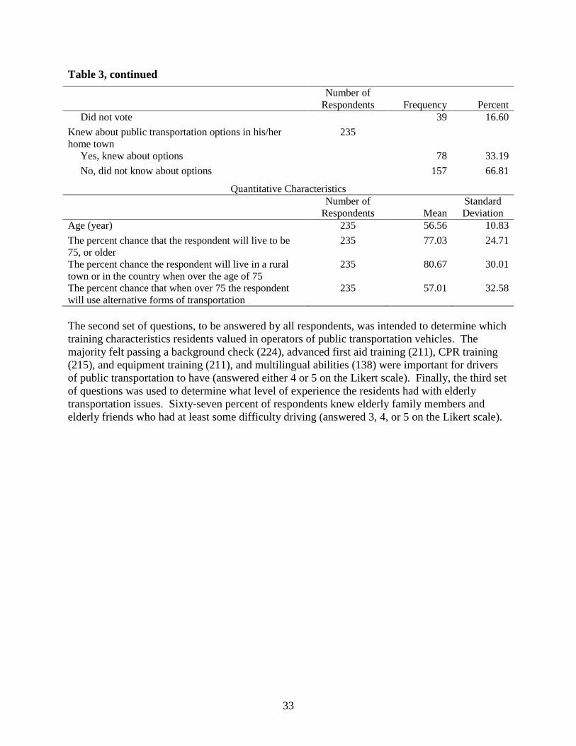
33
Table 3, continued
Number of Respondents Frequency Percent
Did not vote 39 16.60 Knew about public transportation options in his/her home town
235
Yes, knew about options 78 33.19 No, did not know about options 157 66.81
Quantitative Characteristics
Number of
Respondents Mean Standard Deviation
Age (year) 235 56.56 10.83 The percent chance that the respondent will live to be 75, or older
235 77.03 24.71
The percent chance the respondent will live in a rural town or in the country when over the age of 75
235 80.67 30.01
The percent chance that when over 75 the respondent will use alternative forms of transportation
235 57.01 32.58
The second set of questions, to be answered by all respondents, was intended to determine which training characteristics residents valued in operators of public transportation vehicles. The majority felt passing a background check (224), advanced first aid training (211), CPR training (215), and equipment training (211), and multilingual abilities (138) were important for drivers of public transportation to have (answered either 4 or 5 on the Likert scale). Finally, the third set of questions was used to determine what level of experience the residents had with elderly transportation issues. Sixty-seven percent of respondents knew elderly family members and elderly friends who had at least some difficulty driving (answered 3, 4, or 5 on the Likert scale).
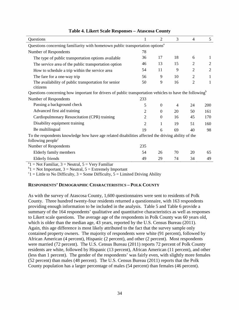
34
Table 4. Likert Scale Responses – Atascosa County
Questions 1 2 3 4 5 Questions concerning familiarity with hometown public transportation optionsa Number of Respondents 78
The type of public transportation options available 36 17 18 6 1 The service area of the public transportation option 46 13 15 2 2 How to schedule a trip within the service area 54 11 9 2 2 The fare for a one-way trip 56 9 10 2 1 The availability of public transportation for senior citizens
50 9 16 2 1
Questions concerning how important for drivers of public transportation vehicles to have the followingb Number of Respondents 233
Passing a background check 5 0 4 24 200 Advanced first aid training 2 0 20 50 161 Cardiopulmonary Resuscitation (CPR) training 2 0 16 45 170 Disability equipment training 2 1 19 51 160 Be multilingual 19 6 69 40 98
To the respondents knowledge how have age related disabilities affected the driving ability of the following peoplec Number of Respondents 235
Elderly family members 54 26 70 20 65 Elderly friends 49 29 74 34 49
a1 = Not Familiar, 3 = Neutral, 5 = Very Familiar b1 = Not Important, 3 = Neutral, 5 = Extremely Important c1 = Little to No Difficulty, 3 = Some Difficulty, 5 = Limited Driving Ability
RESPONDENTS’ DEMOGRAPHIC CHARACTERISTICS – POLK COUNTY As with the survey of Atascosa County, 1,600 questionnaires were sent to residents of Polk County. Three hundred twenty-four residents returned a questionnaire, with 163 respondents providing enough information to be included in the analysis. Table 5 and Table 6 provide a summary of the 164 respondents’ qualitative and quantitative characteristics as well as responses to Likert scale questions. The average age of the respondents in Polk County was 60 years old, which is older than the median age, 43 years, reported by the U.S. Census Bureau (2011). Again, this age difference is most likely attributed to the fact that the survey sample only contained property owners. The majority of respondents were white (91 percent), followed by African American (4 percent), Hispanic (2 percent), and other (2 percent). Most respondents were married (72 percent). The U.S. Census Bureau (2011) reports 72 percent of Polk County residents are white, followed by Hispanic (13 percent), African American (11 percent), and other (less than 1 percent). The gender of the respondents’ was fairly even, with slightly more females (52 percent) than males (48 percent). The U.S. Census Bureau (2011) reports that the Polk County population has a larger percentage of males (54 percent) than females (46 percent).
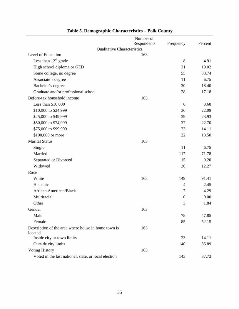
35
Table 5. Demographic Characteristics – Polk County
Number of Respondents Frequency Percent
Qualitative Characteristics Level of Education 163
Less than 12th grade 8 4.91 High school diploma or GED 31 19.02 Some college, no degree 55 33.74 Associate’s degree 11 6.75 Bachelor’s degree 30 18.40 Graduate and/or professional school 28 17.18
Before-tax household income 163 Less than $10,000 6 3.68 $10,000 to $24,999 36 22.09 $25,000 to $49,999 39 23.93 $50,000 to $74,999 37 22.70 $75,000 to $99,999 23 14.11 $100,000 or more 22 13.50
Marital Status 163 Single 11 6.75 Married 117 71.78 Separated or Divorced 15 9.20 Widowed 20 12.27
Race White 163 149 91.41 Hispanic 4 2.45 African American/Black 7 4.29 Multiracial 0 0.00 Other 3 1.84
Gender 163 Male 78 47.85 Female 85 52.15
Description of the area where house in home town is located
163
Inside city or town limits 23 14.11 Outside city limits 140 85.89
Voting History 163 Voted in the last national, state, or local election 143 87.73
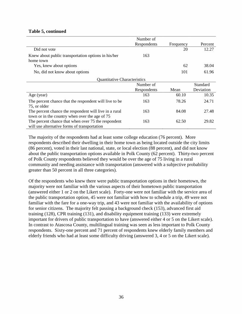
36
Table 5, continued
Number of Respondents Frequency Percent
Did not vote 20 12.27 Knew about public transportation options in his/her home town
163
Yes, knew about options 62 38.04 No, did not know about options 101 61.96
Quantitative Characteristics
Number of
Respondents Mean Standard Deviation
Age (year) 163 60.10 10.35 The percent chance that the respondent will live to be 75, or older
163 78.26 24.71
The percent chance the respondent will live in a rural town or in the country when over the age of 75
163 84.08 27.48
The percent chance that when over 75 the respondent will use alternative forms of transportation
163 62.50 29.82
The majority of the respondents had at least some college education (76 percent). More respondents described their dwelling in their home town as being located outside the city limits (86 percent), voted in their last national, state, or local election (88 percent), and did not know about the public transportation options available in Polk County (62 percent). Thirty-two percent of Polk County respondents believed they would be over the age of 75 living in a rural community and needing assistance with transportation (answered with a subjective probability greater than 50 percent in all three categories).
Of the respondents who knew there were public transportation options in their hometown, the majority were not familiar with the various aspects of their hometown public transportation (answered either 1 or 2 on the Likert scale). Forty-one were not familiar with the service area of the public transportation option, 45 were not familiar with how to schedule a trip, 49 were not familiar with the fare for a one-way trip, and 43 were not familiar with the availability of options for senior citizens. The majority felt passing a background check (153), advanced first aid training (128), CPR training (131), and disability equipment training (133) were extremely important for drivers of public transportation to have (answered either 4 or 5 on the Likert scale). In contrast to Atascosa County, multilingual training was seen as less important to Polk County respondents. Sixty-one percent and 71 percent of respondents knew elderly family members and elderly friends who had at least some difficulty driving (answered 3, 4 or 5 on the Likert scale).
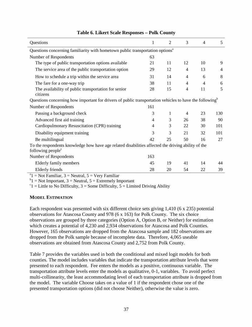
37
Table 6. Likert Scale Responses – Polk County
Questions 1 2 3 4 5 Questions concerning familiarity with hometown public transportation optionsa Number of Respondents 63
The type of public transportation options available 21 11 12 10 9 The service area of the public transportation option 29 12 4 13 4 How to schedule a trip within the service area 31 14 4 6 8 The fare for a one-way trip 38 11 4 4 6 The availability of public transportation for senior citizens
28 15 4 11 5
Questions concerning how important for drivers of public transportation vehicles to have the followingb Number of Respondents 161
Passing a background check 3 1 4 23 130 Advanced first aid training 4 3 26 38 90 Cardiopulmonary Resuscitation (CPR) training 4 3 22 30 101 Disability equipment training 3 3 21 32 101 Be multilingual 42 25 50 16 27
To the respondents knowledge how have age related disabilities affected the driving ability of the following peoplec Number of Respondents 163
Elderly family members 45 19 41 14 44 Elderly friends 28 20 54 22 39
a1 = Not Familiar, 3 = Neutral, 5 = Very Familiar b1 = Not Important, 3 = Neutral, 5 = Extremely Important c1 = Little to No Difficulty, 3 = Some Difficulty, 5 = Limited Driving Ability MODEL ESTIMATION Each respondent was presented with six different choice sets giving 1,410 (6 x 235) potential observations for Atascosa County and 978 (6 x 163) for Polk County. The six choice observations are grouped by three categories (Option A, Option B, or Neither) for estimation which creates a potential of 4,230 and 2,934 observations for Atascosa and Polk Counties. However, 165 observations are dropped from the Atascosa sample and 182 observations are dropped from the Polk sample because of incomplete data. Therefore, 4,065 useable observations are obtained from Atascosa County and 2,752 from Polk County. Table 7 provides the variables used in both the conditional and mixed logit models for both counties. The model includes variables that indicate the transportation attribute levels that were presented to each respondent. Fee enters the models as a positive, continuous variable. The transportation attribute levels enter the models as qualitative, 0-1, variables. To avoid perfect multi-collinearity, the least accommodating level of each transportation attribute is dropped from the model. The variable Choose takes on a value of 1 if the respondent chose one of the presented transportation options (did not choose Neither), otherwise the value is zero.
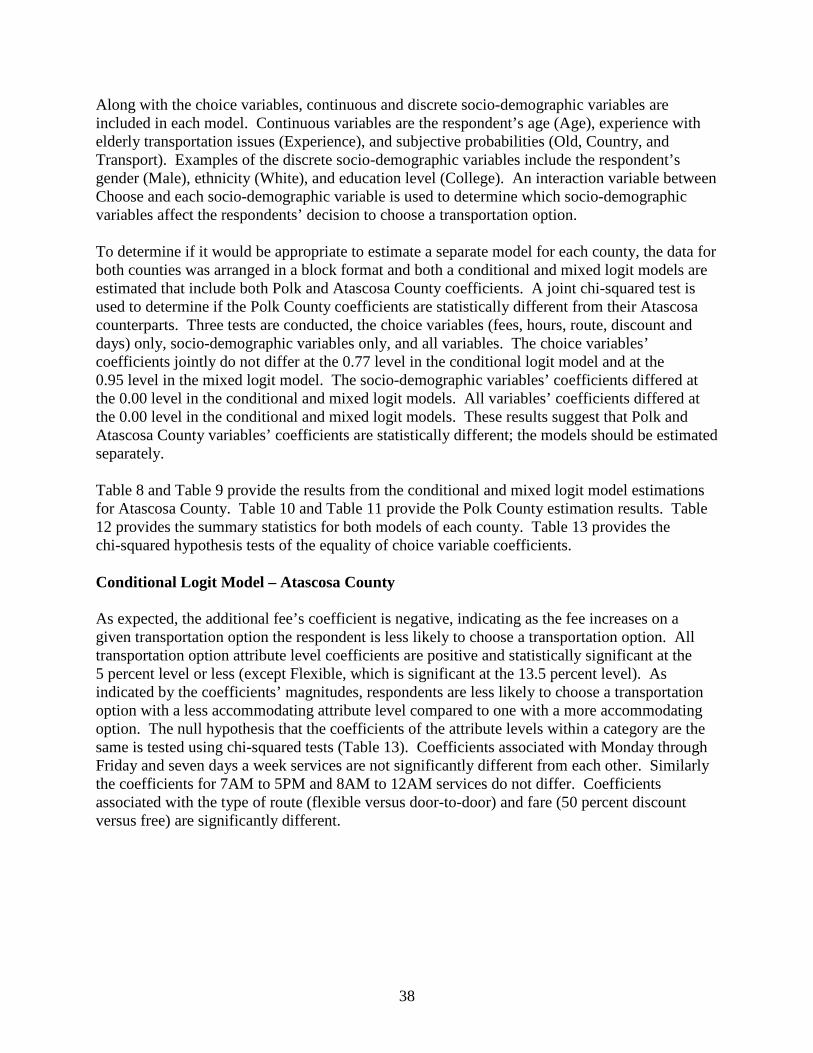
38
Along with the choice variables, continuous and discrete socio-demographic variables are included in each model. Continuous variables are the respondent’s age (Age), experience with elderly transportation issues (Experience), and subjective probabilities (Old, Country, and Transport). Examples of the discrete socio-demographic variables include the respondent’s gender (Male), ethnicity (White), and education level (College). An interaction variable between Choose and each socio-demographic variable is used to determine which socio-demographic variables affect the respondents’ decision to choose a transportation option. To determine if it would be appropriate to estimate a separate model for each county, the data for both counties was arranged in a block format and both a conditional and mixed logit models are estimated that include both Polk and Atascosa County coefficients. A joint chi-squared test is used to determine if the Polk County coefficients are statistically different from their Atascosa counterparts. Three tests are conducted, the choice variables (fees, hours, route, discount and days) only, socio-demographic variables only, and all variables. The choice variables’ coefficients jointly do not differ at the 0.77 level in the conditional logit model and at the 0.95 level in the mixed logit model. The socio-demographic variables’ coefficients differed at the 0.00 level in the conditional and mixed logit models. All variables’ coefficients differed at the 0.00 level in the conditional and mixed logit models. These results suggest that Polk and Atascosa County variables’ coefficients are statistically different; the models should be estimated separately. Table 8 and Table 9 provide the results from the conditional and mixed logit model estimations for Atascosa County. Table 10 and Table 11 provide the Polk County estimation results. Table 12 provides the summary statistics for both models of each county. Table 13 provides the chi-squared hypothesis tests of the equality of choice variable coefficients.
Conditional Logit Model – Atascosa County As expected, the additional fee’s coefficient is negative, indicating as the fee increases on a given transportation option the respondent is less likely to choose a transportation option. All transportation option attribute level coefficients are positive and statistically significant at the 5 percent level or less (except Flexible, which is significant at the 13.5 percent level). As indicated by the coefficients’ magnitudes, respondents are less likely to choose a transportation option with a less accommodating attribute level compared to one with a more accommodating option. The null hypothesis that the coefficients of the attribute levels within a category are the same is tested using chi-squared tests (Table 13). Coefficients associated with Monday through Friday and seven days a week services are not significantly different from each other. Similarly the coefficients for 7AM to 5PM and 8AM to 12AM services do not differ. Coefficients associated with the type of route (flexible versus door-to-door) and fare (50 percent discount versus free) are significantly different.
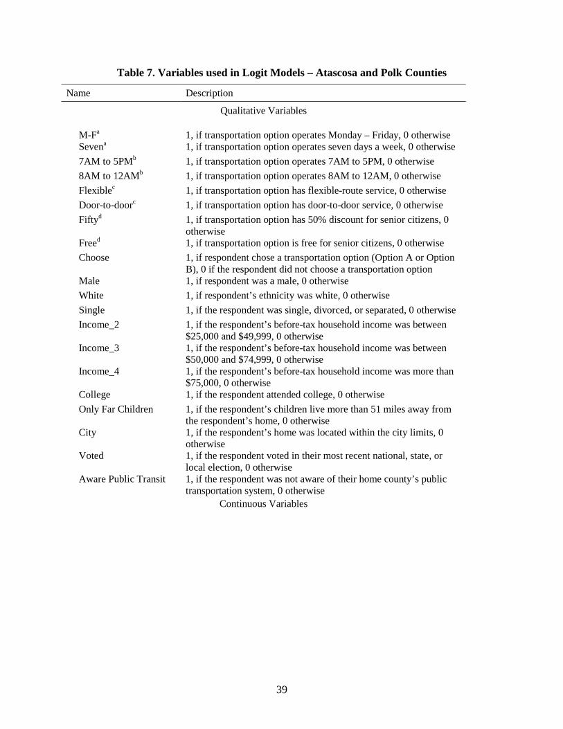
39
Table 7. Variables used in Logit Models – Atascosa and Polk Counties
Name Description Qualitative Variables
M-Fa
1, if transportation option operates Monday – Friday, 0 otherwise
Sevena 1, if transportation option operates seven days a week, 0 otherwise 7AM to 5PMb 1, if transportation option operates 7AM to 5PM, 0 otherwise 8AM to 12AMb 1, if transportation option operates 8AM to 12AM, 0 otherwise Flexiblec 1, if transportation option has flexible-route service, 0 otherwise Door-to-doorc 1, if transportation option has door-to-door service, 0 otherwise Fiftyd 1, if transportation option has 50% discount for senior citizens, 0
otherwise Freed 1, if transportation option is free for senior citizens, 0 otherwise Choose 1, if respondent chose a transportation option (Option A or Option
B), 0 if the respondent did not choose a transportation option Male 1, if respondent was a male, 0 otherwise White 1, if respondent’s ethnicity was white, 0 otherwise Single 1, if the respondent was single, divorced, or separated, 0 otherwise Income_2 1, if the respondent’s before-tax household income was between
$25,000 and $49,999, 0 otherwise Income_3 1, if the respondent’s before-tax household income was between
$50,000 and $74,999, 0 otherwise Income_4 1, if the respondent’s before-tax household income was more than
$75,000, 0 otherwise College 1, if the respondent attended college, 0 otherwise Only Far Children 1, if the respondent’s children live more than 51 miles away from
the respondent’s home, 0 otherwise City 1, if the respondent’s home was located within the city limits, 0
otherwise Voted 1, if the respondent voted in their most recent national, state, or
local election, 0 otherwise Aware Public Transit 1, if the respondent was not aware of their home county’s public
transportation system, 0 otherwise Continuous Variables
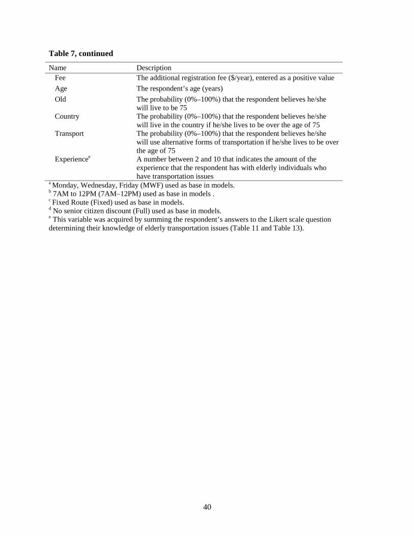
40
Table 7, continued Name Description
Fee The additional registration fee ($/year), entered as a positive value Age The respondent’s age (years) Old The probability (0%–100%) that the respondent believes he/she
will live to be 75 Country The probability (0%–100%) that the respondent believes he/she
will live in the country if he/she lives to be over the age of 75 Transport The probability (0%–100%) that the respondent believes he/she
will use alternative forms of transportation if he/she lives to be over the age of 75
Experiencee A number between 2 and 10 that indicates the amount of the experience that the respondent has with elderly individuals who have transportation issues
a Monday, Wednesday, Friday (MWF) used as base in models. b 7AM to 12PM (7AM–12PM) used as base in models . c Fixed Route (Fixed) used as base in models. d No senior citizen discount (Full) used as base in models. e This variable was acquired by summing the respondent’s answers to the Likert scale question determining their knowledge of elderly transportation issues (Table 11 and Table 13).

41
Table 8. Conditional Logit Model Results – Atascosa County
Variable Coefficient Standard
Error Z
P > |z| WTP
($/Year) Fee ($/year) -0.0491 0.0052 -9.38 0.000
Days of Operation Choice (Base = MWF) M-F 0.2923 0.1098 2.66 0.008 5.96 Seven 0.3750 0.1082 3.47 0.001 7.65
Hours of Operation Choice (Base = 7AM to 12PM) 7AM to 5PM 0.6384 0.1108 5.76 0.000 13.01 8AM to 12AM 0.7306 0.1112 6.57 0.000 14.89
Type of Route Choice (Base = Fixed) Flexible 0.1683 0.1126 1.49 0.135 3.43 Door-to-door 0.7061 0.1090 6.48 0.000 14.40
Senior Citizen Discount Choice (Base = Full) Fifty 0.6384 0.1128 5.66 0.000 13.01 Free 0.9480 0.1124 8.43 0.000 19.33
Qualitative interaction variables Choose*Male -0.2175 0.1637 -1.33 0.184 Choose *White 0.2564 0.1609 1.59 0.111 Choose *Single 1.9717 0.3573 5.52 0.000 Choose *Income_2 0.4630 0.2238 2.07 0.039 Choose *Income_3 1.2849 0.2473 5.20 0.000 Choose *Income_4 1.1205 0.2461 4.55 0.000 Choose *College -0.3807 0.1839 -2.07 0.038 Choose*Only Far Children 0.2541 2.9728 0.12 0.902 Choose*Only Far Children*Age -0.0160 0.0350 -0.46 0.647
Choose *City 1.1146 0.1561 7.14 0.000 Choose *Voted -0.3404 0.2160 -1.58 0.115 Choose * Aware Public Transit 0.2586 0.1658 1.56 0.119
Continuous interaction variables Choose *Age -0.0307 0.0062 -4.98 0.000 Choose *Old -0.0026 0.0035 -0.75 0.451 Choose *Country -0.0010 0.0029 -3.40 0.001 Choose *Transport 0.0068 0.0024 2.81 0.005 Choose *Experience 0.0878 0.0293 3.00 0.003

42
Table 9. Mixed Logit Model Results – Atascosa County
Variable Coefficient Standard
Error z
P > |z| WTP
($/Year) Fee ($/year) -0.0879 0.0089 -9.84 0.000
Days of Operation Choice (Base = MWF) M-F 0.3752 0.2147 1.75 0.081 4.27 Seven 0.5794 0.1887 3.07 0.002 6.59
Hours of Operation Choice (Base = 7AM to 12PM) 7AM to 5PM 0.9878 0.1989 4.92 0.000 11.13 8AM to 12AM 1.1913 0.2250 5.30 0.000 13.56
Type of Route Choice (Base = Fixed) Flexible 0.2519 0.1870 1.35 0.178 2.87 Door-to-door 0.9667 0.2214 4.37 0.000 11.00
Senior Citizen Discount Choice (Base = Full) Fifty 0.9043 0.1887 4.79 0.000 10.29 Free 1.5978 0.2055 7.77 0.000 18.18
Qualitative interaction variables Choose*Male -0.1871 0.2561 -0.73 0.465 Choose *White 0.1599 0.2528 0.63 0.527 Choose *Single 2.1243 0.4779 4.45 0.000 Choose *Income_2 0.1968 0.3419 0.58 0.565 Choose *Income_3 0.9402 0.3928 2.39 0.017 Choose *Income_4 1.0426 0.3906 2.67 0.008 Choose *College -0.2564 0.2858 -0.90 0.370 Choose*Only Far Children 1.9439 3.4596 0.56 0.574 Choose*Only Far Children*Age -0.0451 0.0588 -0.77 0.443
Choose *City 1.2229 0.2505 4.88 0.000 Choose *Voted -0.7159 0.3360 -2.13 0.033 Choose * Aware Public Transit 0.5273 0.2724 1.94 0.053
Continuous interaction variables Choose *Age -0.0294 0.0094 -3.11 0.002 Choose *Old -0.0036 0.0054 -0.67 0.504 Choose *Country -0.0066 0.0044 -1.51 0.131 Choose *Transport 0.0056 0.0037 1.52 0.129 Choose *Experience 0.0813 0.0438 1.85 0.064
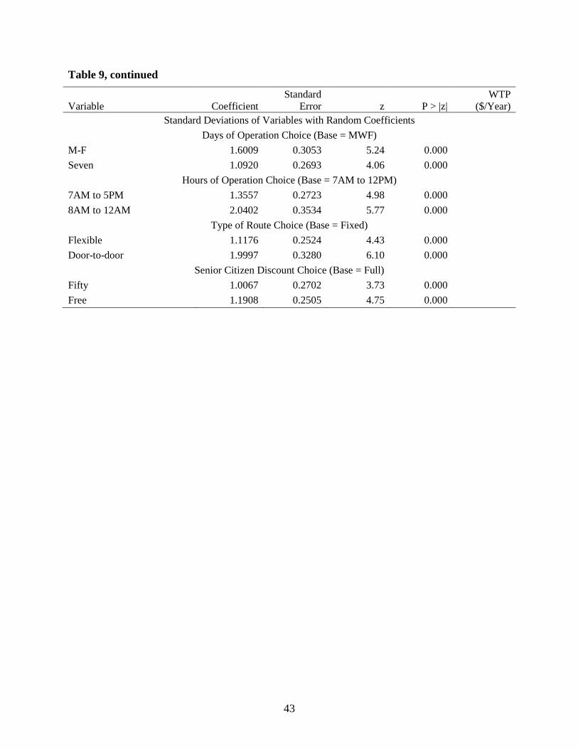
43
Table 9, continued
Variable Coefficient Standard
Error z
P > |z| WTP
($/Year) Standard Deviations of Variables with Random Coefficients
Days of Operation Choice (Base = MWF) M-F 1.6009 0.3053 5.24 0.000 Seven 1.0920 0.2693 4.06 0.000
Hours of Operation Choice (Base = 7AM to 12PM) 7AM to 5PM 1.3557 0.2723 4.98 0.000 8AM to 12AM 2.0402 0.3534 5.77 0.000
Type of Route Choice (Base = Fixed) Flexible 1.1176 0.2524 4.43 0.000 Door-to-door 1.9997 0.3280 6.10 0.000
Senior Citizen Discount Choice (Base = Full) Fifty 1.0067 0.2702 3.73 0.000 Free 1.1908 0.2505 4.75 0.000

44
Table 10. Conditional Logit Model Results – Polk County
Variable Coefficient Standard
Error z
P > |z| WTP
($/Year) Fee ($/year) -0.0583 0.0067 -8.69 0.000
Days of Operation Choice (Base = MWF) M-F 0.5910 0.1394 4.24 0.000 10.14 Seven 0.5941 0.1401 4.24 0.000 10.20
Hours of Operation Choice (Base = 7AM to 12PM) 7AM to 5PM 0.8210 0.1414 5.81 0.000 14.09 8AM to 12AM 0.7383 0.1423 5.19 0.000 12.67
Type of Route Choice (Base = Fixed) Flexible 0.2999 0.1421 2.11 0.035 5.15 Door-to-door 0.7543 0.1347 5.60 0.000 12.95
Senior Citizen Discount Choice (Base = Full) Fifty 0.8108 0.1414 5.73 0.000 13.92 Free 0.9420 0.1431 6.58 0.000 16.17
Qualitative interaction variables Choose*Male -0.7761 0.1867 -4.16 0.000 Choose *White -0.8046 0.3247 -2.48 0.013 Choose *Single -0.7190 0.3701 -1.94 0.052 Choose *Income_2 0.5002 0.2801 1.79 0.074 Choose *Income_3 -0.4744 0.2725 -1.74 0.082 Choose *Income_4 -0.5453 0.2825 -1.93 0.054 Choose *College 0.4260 0.2250 1.89 0.058 Choose*Only Far Children -6.3065 2.0386 -3.09 0.002 Choose*Only Far Children*Age 0.1062 0.0315 3.38 0.001
Choose *City 0.6895 0.2633 2.62 0.009 Choose *Voted -0.2903 0.2900 -1.00 0.317 Choose * Aware Public Transit 0.4073 0.1951 2.09 0.037
Continuous interaction variables Choose *Age -0.0030 0.0082 -0.37 0.709 Choose *Old 0.0004 0.0035 0.11 0.915 Choose *Country -0.0098 0.0035 -2.76 0.006 Choose *Transport -0.0094 0.0033 2.89 0.004 Choose *Experience -0.0532 0.0347 -1.53 0.126
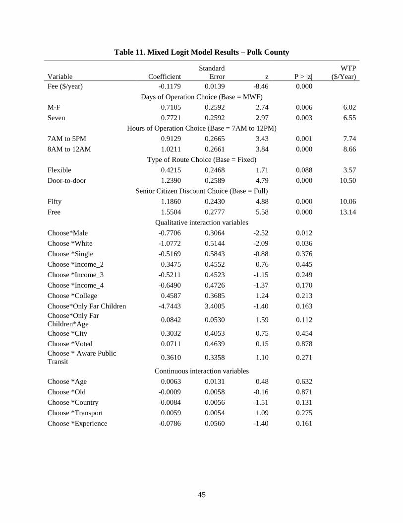
45
Table 11. Mixed Logit Model Results – Polk County
Variable Coefficient Standard
Error z
P > |z| WTP
($/Year) Fee ($/year) -0.1179 0.0139 -8.46 0.000
Days of Operation Choice (Base = MWF) M-F 0.7105 0.2592 2.74 0.006 6.02 Seven 0.7721 0.2592 2.97 0.003 6.55
Hours of Operation Choice (Base = 7AM to 12PM) 7AM to 5PM 0.9129 0.2665 3.43 0.001 7.74 8AM to 12AM 1.0211 0.2661 3.84 0.000 8.66
Type of Route Choice (Base = Fixed) Flexible 0.4215 0.2468 1.71 0.088 3.57 Door-to-door 1.2390 0.2589 4.79 0.000 10.50
Senior Citizen Discount Choice (Base = Full) Fifty 1.1860 0.2430 4.88 0.000 10.06 Free 1.5504 0.2777 5.58 0.000 13.14
Qualitative interaction variables Choose*Male -0.7706 0.3064 -2.52 0.012 Choose *White -1.0772 0.5144 -2.09 0.036 Choose *Single -0.5169 0.5843 -0.88 0.376 Choose *Income_2 0.3475 0.4552 0.76 0.445 Choose *Income_3 -0.5211 0.4523 -1.15 0.249 Choose *Income_4 -0.6490 0.4726 -1.37 0.170 Choose *College 0.4587 0.3685 1.24 0.213 Choose*Only Far Children -4.7443 3.4005 -1.40 0.163 Choose*Only Far Children*Age 0.0842 0.0530 1.59 0.112
Choose *City 0.3032 0.4053 0.75 0.454 Choose *Voted 0.0711 0.4639 0.15 0.878 Choose * Aware Public Transit 0.3610 0.3358 1.10 0.271
Continuous interaction variables Choose *Age 0.0063 0.0131 0.48 0.632 Choose *Old -0.0009 0.0058 -0.16 0.871 Choose *Country -0.0084 0.0056 -1.51 0.131 Choose *Transport 0.0059 0.0054 1.09 0.275 Choose *Experience -0.0786 0.0560 -1.40 0.161
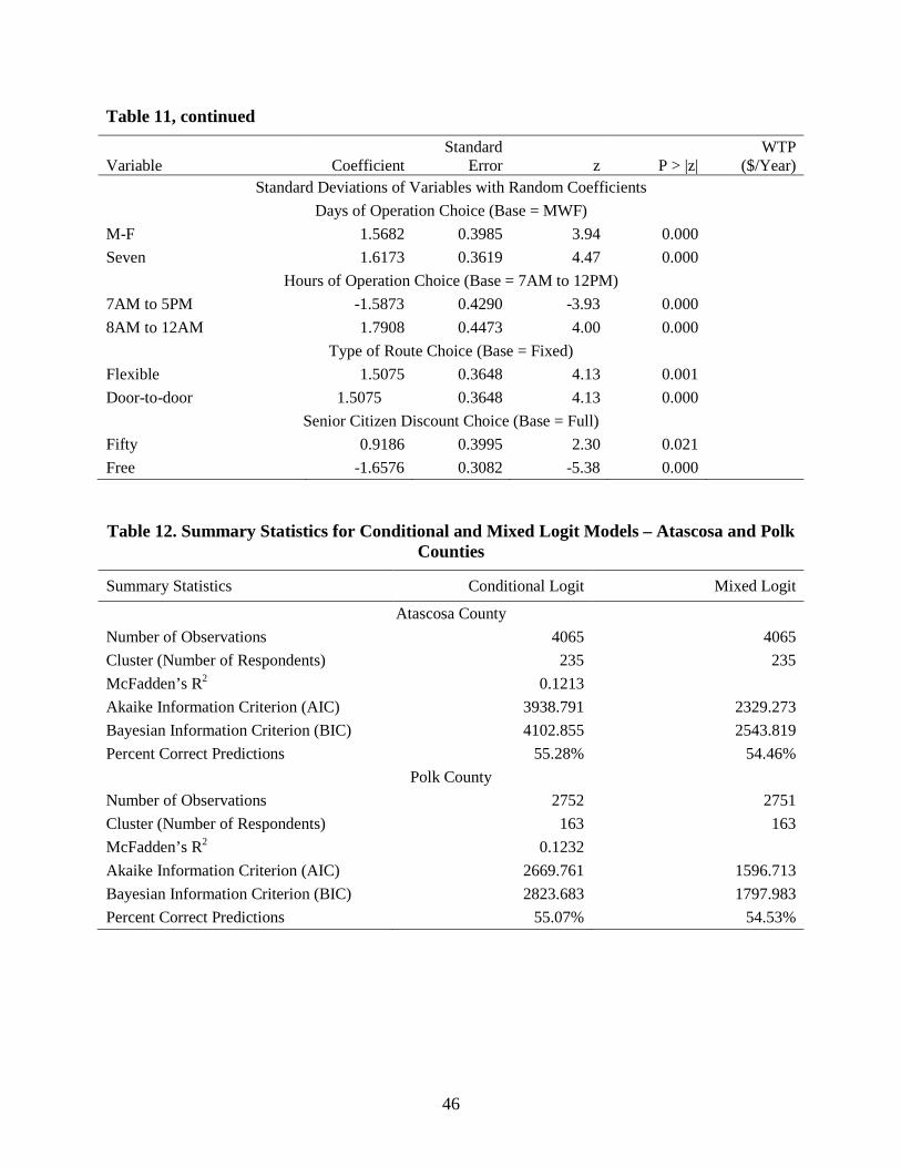
46
Table 11, continued
Variable Coefficient Standard
Error z
P > |z| WTP
($/Year) Standard Deviations of Variables with Random Coefficients
Days of Operation Choice (Base = MWF) M-F 1.5682 0.3985 3.94 0.000 Seven 1.6173 0.3619 4.47 0.000
Hours of Operation Choice (Base = 7AM to 12PM) 7AM to 5PM -1.5873 0.4290 -3.93 0.000 8AM to 12AM 1.7908 0.4473 4.00 0.000
Type of Route Choice (Base = Fixed) Flexible 1.5075 0.3648 4.13 0.001 Door-to-door 1.5075 0.3648 4.13 0.000
Senior Citizen Discount Choice (Base = Full) Fifty 0.9186 0.3995 2.30 0.021 Free -1.6576 0.3082 -5.38 0.000 Table 12. Summary Statistics for Conditional and Mixed Logit Models – Atascosa and Polk
Counties
Summary Statistics Conditional Logit Mixed Logit Atascosa County
Number of Observations 4065 4065 Cluster (Number of Respondents) 235 235 McFadden’s R2 0.1213 Akaike Information Criterion (AIC) 3938.791 2329.273 Bayesian Information Criterion (BIC) 4102.855 2543.819 Percent Correct Predictions 55.28% 54.46%
Polk County Number of Observations 2752 2751 Cluster (Number of Respondents) 163 163 McFadden’s R2 0.1232 Akaike Information Criterion (AIC) 2669.761 1596.713 Bayesian Information Criterion (BIC) 2823.683 1797.983 Percent Correct Predictions 55.07% 54.53%
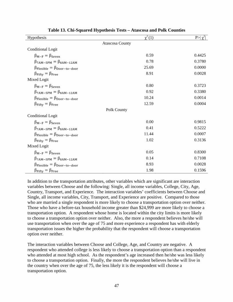
47
Table 13. Chi-Squared Hypothesis Tests – Atascosa and Polk Counties Hypothesis χ2 (1) P>| χ2|
Atascosa County Conditional Logit
βM−F = βSeven 0.59 0.4425 β7AM−5PM = β8AM−12AM 0.78 0.3780 βFlexible = βDoor−to−door 25.69 0.0000 βFifty = βFree 8.91 0.0028
Mixed Logit βM−F = βSeven 0.80 0.3723 β7AM−5PM = β8AM−12AM 0.92 0.3380 βFlexible = βDoor−to−door 10.24 0.0014 βFifty = βFree 12.59 0.0004
Polk County Conditional Logit
βM−F = βSeven 0.00 0.9815 β7AM−5PM = β8AM−12AM 0.41 0.5222 βFlexible = βDoor−to−door 11.44 0.0007 βFifty = βFree 1.02 0.3136
Mixed Logit βM−F = βSeven 0.05 0.8300 β7AM−5PM = β8AM−12AM 0.14 0.7108 βFlexible = βDoor−to−door 8.93 0.0028 βFifty = βFree 1.98 0.1596
In addition to the transportation attributes, other variables which are significant are interaction variables between Choose and the following: Single, all income variables, College, City, Age, Country, Transport, and Experience. The interaction variables’ coefficients between Choose and Single, all income variables, City, Transport, and Experience are positive. Compared to those who are married a single respondent is more likely to choose a transportation option over neither. Those who have a before-tax household income greater than $24,999 are more likely to choose a transportation option. A respondent whose home is located within the city limits is more likely to choose a transportation option over neither. Also, the more a respondent believes he/she will use transportation when over the age of 75 and more experience a respondent has with elderly transportation issues the higher the probability that the respondent will choose a transportation option over neither. The interaction variables between Choose and College, Age, and Country are negative. A respondent who attended college is less likely to choose a transportation option than a respondent who attended at most high school. As the respondent’s age increased then he/she was less likely to choose a transportation option. Finally, the more the respondent believes he/she will live in the country when over the age of 75, the less likely it is the respondent will choose a transportation option.
48
Variables that are not significant in the conditional model are the interaction variables between Choose and Male, White, Only Far Children, Only Far Children*Age, Voted, Aware Public Transit, and Old. These characteristics (the respondent’s gender and ethnicity, where the respondent’s children lived, whether or not he/she voted, knew about public transportation in their home town and whether the respondent believed he/she would live to be over the age of 75) are not statistically significant in impacting a respondent’s decision to choose a transportation option.
Willingness-to-Pay. All mean WTPs are positive (Table 8), indicating respondents are willing to pay more for the attributes in the model than their base level. In general, respondents are willing to pay the least for the less accommodating level of an attribute, and more for the more accommodating levels. The conditional logit model shows Atascosa County residents are willing to annually pay:
1) $8 more for a seven days a week service and $6 more for a Monday through Friday
service than a Monday, Wednesday, Friday service; 2) $15 more for an 8AM to 12 midnight service and $13 more for a 7AM to 5PM service
than a 7AM to 12AM service; 3) $14 more for a door-to-door route and $3 more for a flexible route than a fixed route;
and 4) $19 more for an option with free fare for senior citizens and $13 more for an option
that gives a 50 percent discount for senior citizens than an option that gives no discount.
Conditional Logit Model – Polk County Again, the additional fee’s coefficient is negative; as the fee increases on the transportation option then the respondent is less likely to choose the option (Table 10). Similar to the Atascosa County model, all transportation option attribute level coefficients are positive and statistically significant. The one exception is the coefficient for a flexible route, which is not significant in the Atascosa model but is now significant at the 5 percent level. When considering only magnitudes of the coefficients, respondents are more likely to choose a transportation option with a more accommodating attribute level than a less accommodating one. The only exception is in the case of hours of operation. Only the route attribute levels’ coefficients (Flexible versus Door-to-Door) are statistically different from one another (Table 13). Interaction variables that are significant are interactions between Choose and the following: Male, White, Only Far Children, Only Far Children*Age, City, Aware Public Transit, Country, and Transport. Interaction variables’ coefficients between Choose and City, and Aware Public Transit are positive. A respondent whose home is within the city limits is more likely to choose a transportation option over neither. A respondent who is aware of the transportation options in Polk County is more likely to choose a transportation option over neither. Interaction variables between Choose and Male, White, Country, and Transport are negative. A male respondent is less likely to choose a transportation option than a female respondent. Compared to other ethnicities, a white respondent is less likely to choose a transportation option
49
over neither. Finally, the more the respondent believes he/she will live in the country or use alternative forms of transportation when over the age of 75, the less likely it is the respondent will choose a transportation option. The interaction between Choose and Only Far Children is difficult to interpret. This is because the coefficient associated with the interaction between Choose and Only Far Children*Age is positive, but the coefficient associated with the interaction between Choose and Only Far Children is negative. The effect of these two coefficients along with age is necessary to determine the overall effect of Only Far Children on the probability of a respondent choosing a transportation option. Variables that are not significant in the conditional model are the interaction variables between Choose and Single, all income variables, College, Voted, Age, Old, and Experience. These characteristics (the respondent’s marital status, age and income, whether the respondent attended college, whether or not he/she voted, and whether the respondent believed he/she would live to be over the age of 75) are not statistically significant in impacting a respondent’s decision to choose a transportation option. Willingness-to-Pay. Respondents, generally, are willing to pay the least for the less accommodating and more for more accommodating levels (Table 10). The conditional logit model shows Polk County residents’ annual mean WTP is:
1) $10 more for a seven days a week service and $10 for a Monday through Friday
service than a Monday, Wednesday, Friday service; 2) $13 more for an 8AM to 12 midnight service and $14 more for a 7AM to 5PM service
than a 7AM to 12AM service; 3) $13 more for a door-to-door route and $5 more for a flexible route than a fixed route;
and 4) $16 more for an option with free fare for senior citizens and $14 more for an option
that gives a 50 percent discount for senior citizens than an option that gives no discount.
Mixed Logit Model – Atascosa County The results from the mixed logit model (Table 9) are similar to the conditional logit model, in terms of the transportation attributes. The additional fee’s coefficient is statistically significant and negative. All transportation option attribute level coefficients are positive and are statistically significant, except for M-F and Flexible. The coefficient inferences remain similar. These attributes increase the probability that a respondent will choose a transportation option over another. Also, similar to the conditional model, coefficients for the route and senior citizen discount attributes are statistically different from each other (Table 13). Interactions between Choose and Single, Income_3, Income_4, City, Voted, Aware Public Transit, and Age are significant at the 5 percent level. Differences between the conditional logit and mixed logit in terms of significance are noted. The interaction variable between Choose and Experience, which was significant at the 5 percent level in the conditional logit is significant at
50
the 6 percent level in the mixed logit model. Further, the interactions between Choose and Income_2, College, Country, and Transport, and are not significant in the mixed logit model, but are significant in the conditional logit model. Interactions between Choose and Aware Public Transit and Voted are not significant in the conditional model, but are significant in the mixed logit model. Interaction variables between Choose and Male, White, Only Far Children, Only Far Children*Age, and Old are not significant in the conditional logit model and are also not significant in the mixed logit model. All coefficients for the variables in the mixed logit model have the same sign as in the conditional logit model, resulting in the same inference.
Willingness-to-Pay. As in the conditional model, the coefficients for transportation option attributes in the mixed model were translated into yearly WTP (Table 9). The resulting mean WTPs are generally lower than the WTPs calculated for the conditional logit model. The Atascosa County resident population is willing to annually pay:
1) $7 more for a seven days a week service and $4 more for a Monday through Friday
service than a Monday, Wednesday, Friday service; 2) $14 more for an 8AM to 12 midnight service and $11 more for an 8AM to 5PM
service than a 7AM to 12AM service; 3) $11 more for a door-to-door route and $3 more for a flexible route than a fixed route;
and 4) $18 more for an option with free fare for senior citizens and $10 more for an option
that gives a 50 percent discount for senior citizens than an option that gives no discount.
One advantage to the mixed logit model is the percentages of the population and sample (see Methodology for explanation of population versus sample), which prefer the attribute over the base attribute (indicated by a positive WTP) can be calculated:
1) 59 percent of the resident population and 67 percent of the resident sample prefer
Monday through Friday service over Monday, Wednesday, Friday service; 2) 70 percent of resident population and 84 percent of the resident sample prefer seven
days a week service over Monday, Wednesday, Friday service; 3) 76 percent resident population and 90 percent of the resident sample prefer 7AM to
5PM service over 7AM to 12PM service; 4) 72 percent resident population and 79 percent of the resident sample prefer 8AM to
12AM service over 7AM to 12PM service; 5) 59 percent of the resident population and 66 percent of the resident sample prefer a
flexible route over a fixed route; 6) 69 percent of the resident population and 78 percent of the resident sample prefer a
door-to-door route over a fixed route; 7) 82 percent of the resident population and 95 percent of the resident sample prefer a
50 percent discount over no fare discount for senior citizens; and 8) 91 percent of the resident population and 99 percent of the resident sample prefer free
fare over no fare discount for senior citizens.
51
Mixed Logit Model – Polk County Results from the Polk County mixed logit model (Table 11) are similar to the conditional logit model, for the transportation options. The additional fee’s coefficient is statistically significant and negative. All transportation option attribute level coefficients are positive and statistically significant, except Flexible. Coefficient inferences, therefore, remain the same. These attributes increase the probability that a respondent will choose a transportation option over another. Also, only the coefficients of route attribute category are statistically different from each other (Table 13). Only Interactions between Choose and Male, and Choose and White are significant at the 5 percent level. The main difference between the conditional logit and mixed logit model is that all coefficients (excluding the interaction variables between Choose and Male, and White) that are significant in the conditional model at the 5 percent level are not significant using mixed logit estimation. Most coefficients for the variables in the mixed logit model have the same sign as in the conditional model, resulting in the same inference. The coefficients of the interaction variables between Choose and Voted, Age, Old, and Transport are opposite in sign from the conditional model.
Willingness-to-Pay. The Polk County resident population’s mean annual WTP are:
1) $7 more for a seven days a week service and $6 more for a Monday through Friday
service than a Monday, Wednesday, Friday service; 2) $9 more for an 8AM to 12 midnight service and $8 more for an 8AM to 5PM service
than a 7AM to 12PM service; 3) $11 more for a door-to-door route and $4 more for a flexible route than a fixed route;
and 4) $13 more for an option with free fare for senior citizens and $10 more for an option
that gives a 50 percent discount for senior citizens than an option that gives no discount.
The percentages of the population and sample (see Methodology for explanation of population versus sample) that prefer the attribute over the base attribute are:
1) 67 percent of the resident population and 79 percent of the resident sample prefer Monday through Friday service over Monday, Wednesday, Friday service;
2) 68 percent of the resident population and 77 percent of the resident sample prefer seven days a week service over Monday, Wednesday, Friday service;
3) 71 percent of the resident population and 84 percent of the resident sample prefer 7AM to 5PM service over 7AM to 12PM service;
4) 72 percent of the resident population and 79 percent of the resident sample prefer 8AM to 12AM service over 7AM to 12PM service;
5) 62 percent of the resident population and 69 percent of the resident sample prefer a flexible route over a fixed route;
6) 79 percent of the resident population and 88 percent of the resident sample prefer a door-to-door route over a fixed route;
52
7) 90 percent of the resident population and 99 percent of the resident sample prefer a 50 percent discount over no fare discount for senior citizens; and
8) 83 percent of the resident population and 91 percent of the resident sample prefer free fare over no fare discount for senior citizens.
DIFFERENCES BETWEEN THE CONDITIONAL LOGIT AND MIXED LOGIT MODELS There are significant differences between the Atascosa County and Polk County mixed and conditional logit models. Although the estimated variable coefficients maintain a similar magnitude and the same sign between both models, variables which are significant in the conditional model do not maintain their significance in the mixed logit model. Also, in Atascosa County the population’s mean WTPs are generally lower for the mixed logit model than for the conditional logit model. Specifically, the highest differences in WTP are seen for seven days a week service (40 percent less), flexible and door-to-door route (20 percent and 31 percent less), and 50 percent fare discount for senior citizens (26 percent less). Similar to Atascosa County, there are notable differences between the WTPs in Polk County’s mixed and conditional logit models. On average, there is almost a 50 percent difference between the mixed and conditional logit mean WTP. The highest difference in WTP (82 percent) is found between the mean WTP for the 7AM to 5PM hours of operation level. In the case of Atascosa County, both the conditional and mixed logit models have about the same correct predictions (55 percent and 54 percent). The conditional logit model slightly outperforms the mixed logit model with 749 correct predictions compared to 738 for the mixed logit model. For Polk County again, the conditional logit model slightly outperforms the mixed logit model with 505 correct predictions compared to 500. In both the Atascosa County and Polk County models, the standard deviations of the variables with random coefficients in the mixed logit model are highly significant (see Standard Deviations of Variables with Random Coefficients section in Table 9 and Table 10). This significance indicates these coefficients vary within both populations. Based on these analyses, it is concluded that the mixed logit model is preferred to the conditional logit model for both Atascosa and Polk County.
CHAPTER 5. FINDINGS – PARKER COUNTY SURVEY Because the results for Atascosa and Polk Counties were similar and because the research team had saved money by conducting its own survey mailings rather than contracting mailing services, the team received permission to survey a third county. Parker County was chosen because it is a more populated county in a different region of Texas (north-central) with different socio-cultural histories. Further, Parker County is at the fringe of the Dallas-Fort Worth metro area with a large commuter base as well as a rapidly growing elderly population (53 percent increase between 2000 and 2010). The transit district serving Parker County, Public Transit Services, has an interest in improving the public transportation systems. RESPONDENTS’ DEMOGRAPHIC CHARACTERISTICS – PARKER COUNTY One thousand six hundred questionnaires were sent to Parker County residents, 396 were returned, with 260 respondents providing enough information to be included in the analysis.
53
Table 14 and Table 15 summarize the 260 respondents’ qualitative and quantitative characteristics and their responses to Likert scale questions. Average age of the respondents in Parker County was 54 years old, which is older than the median age, 39 years, reported by the U.S. Census Bureau (2011). This age difference is most likely attributed to the fact that the survey sample only contained property owners, which is generally an older age group. The majority of respondents were white (96 percent). Census data indicate 85 percent of Parker County residents are white, and 11 percent are Hispanic (U.S. Census Bureau 2011). Most respondents were married (75 percent), which is higher than the reported husband-wife family households (62 percent) reported by the U.S. Census Bureau (2011). Parker County’s population is approximately 51 percent male and 49 percent female (U.S. Census Bureau 2011), and 48 percent of respondents were male and 52 percent female. A majority of respondents had at least some college education (85 percent). Most respondents described their dwelling in their home town as being located outside the city limits (72 percent) and voted in their last national, state, or local election (84 percent). As compared to respondents in Atascosa and Polk Counties, Parker County respondents were more aware of local transit services with 55 percent of respondents knowing about the public transportation options available in Parker County.
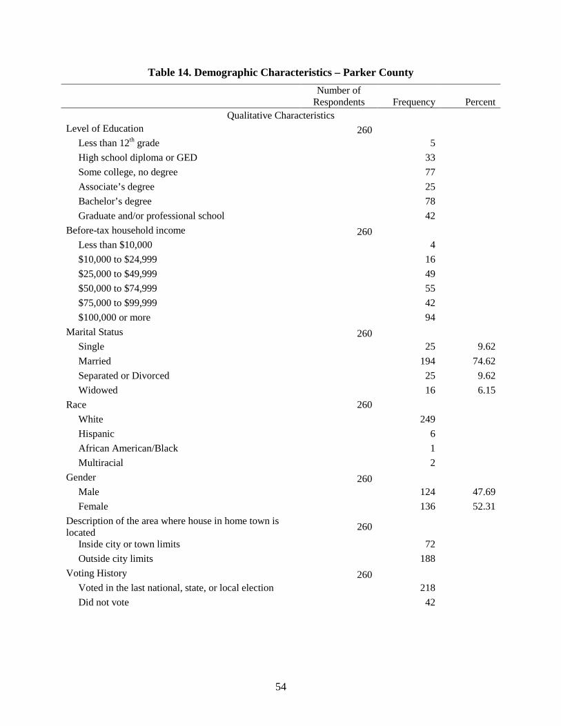
54
Table 14. Demographic Characteristics – Parker County
Number of Respondents Frequency Percent
Qualitative Characteristics Level of Education 260
Less than 12th grade
5 High school diploma or GED 33 Some college, no degree 77 Associate’s degree 25 Bachelor’s degree 78 Graduate and/or professional school 42
Before-tax household income 260 Less than $10,000 4 $10,000 to $24,999 16 $25,000 to $49,999 49 $50,000 to $74,999 55 $75,000 to $99,999 42 $100,000 or more 94
Marital Status 260 Single 25 9.62 Married 194 74.62 Separated or Divorced 25 9.62 Widowed 16 6.15
Race 260 White 249 Hispanic 6 African American/Black 1 Multiracial 2
Gender 260 Male 124 47.69 Female 136 52.31
Description of the area where house in home town is located 260
Inside city or town limits 72 Outside city limits 188
Voting History 260 Voted in the last national, state, or local election 218 Did not vote 42
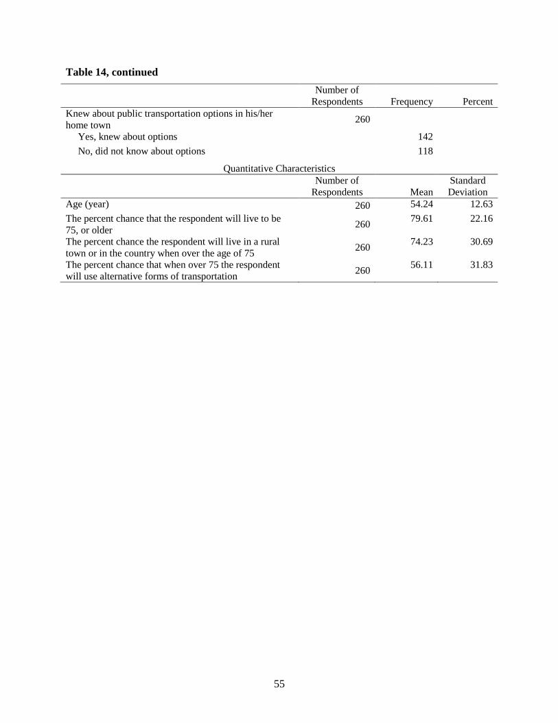
55
Table 14, continued
Number of Respondents Frequency Percent
Knew about public transportation options in his/her home town 260
Yes, knew about options 142 No, did not know about options 118
Quantitative Characteristics
Number of
Respondents Mean Standard Deviation
Age (year) 260 54.24 12.63 The percent chance that the respondent will live to be 75, or older 260 79.61 22.16
The percent chance the respondent will live in a rural town or in the country when over the age of 75 260 74.23 30.69
The percent chance that when over 75 the respondent will use alternative forms of transportation 260 56.11 31.83
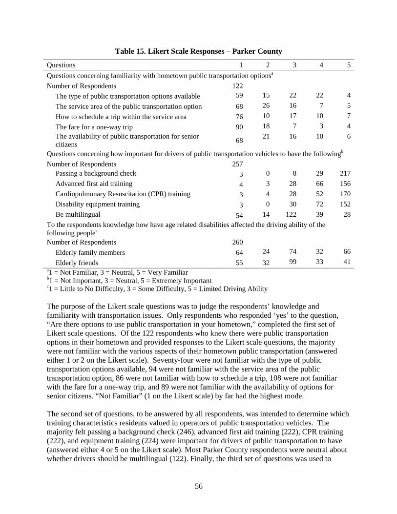
56
Table 15. Likert Scale Responses – Parker County
Questions 1 2 3 4 5 Questions concerning familiarity with hometown public transportation optionsa Number of Respondents 122
The type of public transportation options available 59 15 22 22 4 The service area of the public transportation option 68 26 16 7 5 How to schedule a trip within the service area 76 10 17 10 7 The fare for a one-way trip 90 18 7 3 4 The availability of public transportation for senior citizens 68 21 16 10 6
Questions concerning how important for drivers of public transportation vehicles to have the followingb Number of Respondents 257
Passing a background check 3 0 8 29 217 Advanced first aid training 4 3 28 66 156 Cardiopulmonary Resuscitation (CPR) training 3 4 28 52 170 Disability equipment training 3 0 30 72 152 Be multilingual 54 14 122 39 28
To the respondents knowledge how have age related disabilities affected the driving ability of the following peoplec Number of Respondents 260
Elderly family members 64 24 74 32 66 Elderly friends 55 32 99 33 41
a1 = Not Familiar, 3 = Neutral, 5 = Very Familiar b1 = Not Important, 3 = Neutral, 5 = Extremely Important c1 = Little to No Difficulty, 3 = Some Difficulty, 5 = Limited Driving Ability The purpose of the Likert scale questions was to judge the respondents’ knowledge and familiarity with transportation issues. Only respondents who responded ‘yes’ to the question, “Are there options to use public transportation in your hometown,” completed the first set of Likert scale questions. Of the 122 respondents who knew there were public transportation options in their hometown and provided responses to the Likert scale questions, the majority were not familiar with the various aspects of their hometown public transportation (answered either 1 or 2 on the Likert scale). Seventy-four were not familiar with the type of public transportation options available, 94 were not familiar with the service area of the public transportation option, 86 were not familiar with how to schedule a trip, 108 were not familiar with the fare for a one-way trip, and 89 were not familiar with the availability of options for senior citizens. “Not Familiar” (1 on the Likert scale) by far had the highest mode.
The second set of questions, to be answered by all respondents, was intended to determine which training characteristics residents valued in operators of public transportation vehicles. The majority felt passing a background check (246), advanced first aid training (222), CPR training (222), and equipment training (224) were important for drivers of public transportation to have (answered either 4 or 5 on the Likert scale). Most Parker County respondents were neutral about whether drivers should be multilingual (122). Finally, the third set of questions was used to
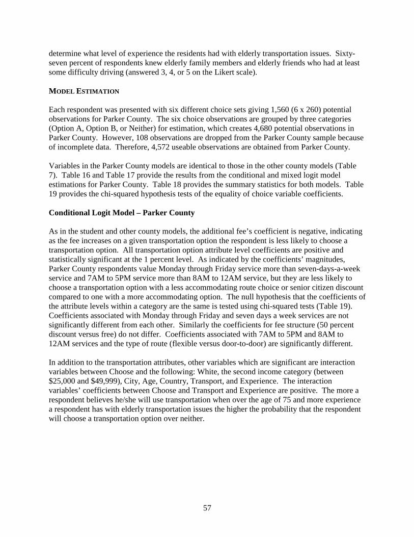
57
determine what level of experience the residents had with elderly transportation issues. Sixty-seven percent of respondents knew elderly family members and elderly friends who had at least some difficulty driving (answered 3, 4, or 5 on the Likert scale).
MODEL ESTIMATION Each respondent was presented with six different choice sets giving 1,560 (6 x 260) potential observations for Parker County. The six choice observations are grouped by three categories (Option A, Option B, or Neither) for estimation, which creates 4,680 potential observations in Parker County. However, 108 observations are dropped from the Parker County sample because of incomplete data. Therefore, 4,572 useable observations are obtained from Parker County. Variables in the Parker County models are identical to those in the other county models (Table 7). Table 16 and Table 17 provide the results from the conditional and mixed logit model estimations for Parker County. Table 18 provides the summary statistics for both models. Table 19 provides the chi-squared hypothesis tests of the equality of choice variable coefficients.
Conditional Logit Model – Parker County As in the student and other county models, the additional fee’s coefficient is negative, indicating as the fee increases on a given transportation option the respondent is less likely to choose a transportation option. All transportation option attribute level coefficients are positive and statistically significant at the 1 percent level. As indicated by the coefficients’ magnitudes, Parker County respondents value Monday through Friday service more than seven-days-a-week service and 7AM to 5PM service more than 8AM to 12AM service, but they are less likely to choose a transportation option with a less accommodating route choice or senior citizen discount compared to one with a more accommodating option. The null hypothesis that the coefficients of the attribute levels within a category are the same is tested using chi-squared tests (Table 19). Coefficients associated with Monday through Friday and seven days a week services are not significantly different from each other. Similarly the coefficients for fee structure (50 percent discount versus free) do not differ. Coefficients associated with 7AM to 5PM and 8AM to 12AM services and the type of route (flexible versus door-to-door) are significantly different. In addition to the transportation attributes, other variables which are significant are interaction variables between Choose and the following: White, the second income category (between $25,000 and $49,999), City, Age, Country, Transport, and Experience. The interaction variables’ coefficients between Choose and Transport and Experience are positive. The more a respondent believes he/she will use transportation when over the age of 75 and more experience a respondent has with elderly transportation issues the higher the probability that the respondent will choose a transportation option over neither.
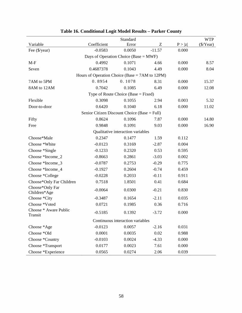
58
Table 16. Conditional Logit Model Results – Parker County
Variable Coefficient Standard
Error Z
P > |z| WTP
($/Year) Fee ($/year) -0.0583 0.0050 -11.57 0.000
Days of Operation Choice (Base = MWF) M-F 0.4992 0.1071 4.66 0.000 8.57 Seven 0.4687378 0.1043 4.49 0.000 8.04
Hours of Operation Choice (Base = 7AM to 12PM) 7AM to 5PM 0.8954 0.1078 8.31 0.000 15.37 8AM to 12AM 0.7042 0.1085 6.49 0.000 12.08
Type of Route Choice (Base = Fixed) Flexible 0.3098 0.1055 2.94 0.003 5.32 Door-to-door 0.6420 0.1040 6.18 0.000 11.02
Senior Citizen Discount Choice (Base = Full) Fifty 0.8624 0.1096 7.87 0.000 14.80 Free 0.9848 0.1091 9.03 0.000 16.90
Qualitative interaction variables Choose*Male 0.2347 0.1477 1.59 0.112 Choose *White -0.0123 0.3169 -2.87 0.004 Choose *Single -0.1233 0.2320 0.53 0.595 Choose *Income_2 -0.8663 0.2861 -3.03 0.002 Choose *Income_3 -0.0787 0.2753 -0.29 0.775 Choose *Income_4 -0.1927 0.2604 -0.74 0.459 Choose *College -0.0228 0.2033 -0.11 0.911 Choose*Only Far Children 0.7518 1.8501 0.41 0.684 Choose*Only Far Children*Age -0.0064 0.0300 -0.21 0.830
Choose *City -0.3487 0.1654 -2.11 0.035 Choose *Voted 0.0721 0.1985 0.36 0.716 Choose * Aware Public Transit -0.5185 0.1392 -3.72 0.000
Continuous interaction variables Choose *Age -0.0123 0.0057 -2.16 0.031 Choose *Old 0.0001 0.0035 0.02 0.988 Choose *Country -0.0103 0.0024 -4.33 0.000 Choose *Transport 0.0177 0.0023 7.61 0.000 Choose *Experience 0.0565 0.0274 2.06 0.039

59
Table 17. Mixed Logit Model Results – Parker County
Variable Coefficient Standard
Error z
P > |z| WTP
($/Year) Fee ($/year) -0.0994 0.0090 -11.09 0.000
Days of Operation Choice (Base = MWF) M-F 0.7093 0.1697 4.18 0.000 7.14 Seven 0.7109 0.1890 3.76 0.000 7.15
Hours of Operation Choice (Base = 7AM to 12PM) 7AM to 5PM 1.2862 0.1938 6.64 0.000 12.94 8AM to 12AM 0.9047 0.1895 4.77 0.000 9.10
Type of Route Choice (Base = Fixed) Flexible 0.2646 0.1831 1.45 0.148 2.66 Door-to-door 0.8788 0.1955 4.49 0.000 8.84
Senior Citizen Discount Choice (Base = Full) Fifty 1.2166 0.2066 5.89 0.000 12.24 Free 1.3542 0.1941 6.98 0.000 13.62
Qualitative interaction variables Choose*Male 0.6548 0.2537 2.58 0.010 Choose *White -1.1678 0.5252 -2.22 0.026 Choose *Single 0.4211 0.4509 0.93 0.350 Choose *Income_2 -0.8854 0.5129 -1.73 0.084 Choose *Income_3 -0.1202 0.4752 -0.25 0.800 Choose *Income_4 -0.1980 0.4598 -0.43 0.667 Choose *College -0.0564 0.3183 -0.18 0.859 Choose*Only Far Children -2.1180 2.8652 -0.74 0.460 Choose*Only Far Children*Age 0.0393 0.0469 0.84 0.402
Choose *City -0.5203 0.2574 -2.02 0.043 Choose *Voted 0.2670 0.3061 0.87 0.383 Choose * Aware Public Transit -0.5715 0.2248 -2.54 0.011
Continuous interaction variables Choose *Age -0.0173 0.0091 -1.91 0.056 Choose *Old 0.0017 0.0056 0.30 0.763 Choose *Country -0.0135 0.0038 -3.57 0.000 Choose *Transport 0.0163 0.0042 3.85 0.000 Choose *Experience 0.1041 0.0438 2.38 0.017
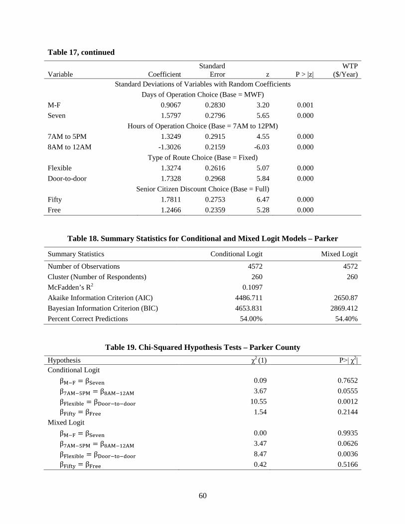
60
Table 17, continued
Variable Coefficient Standard
Error z
P > |z| WTP
($/Year) Standard Deviations of Variables with Random Coefficients
Days of Operation Choice (Base = MWF) M-F 0.9067 0.2830 3.20 0.001 Seven 1.5797 0.2796 5.65 0.000
Hours of Operation Choice (Base = 7AM to 12PM) 7AM to 5PM 1.3249 0.2915 4.55 0.000 8AM to 12AM -1.3026 0.2159 -6.03 0.000
Type of Route Choice (Base = Fixed) Flexible 1.3274 0.2616 5.07 0.000 Door-to-door 1.7328 0.2968 5.84 0.000
Senior Citizen Discount Choice (Base = Full) Fifty 1.7811 0.2753 6.47 0.000 Free 1.2466 0.2359 5.28 0.000
Table 18. Summary Statistics for Conditional and Mixed Logit Models – Parker
Summary Statistics Conditional Logit Mixed Logit Number of Observations 4572 4572 Cluster (Number of Respondents) 260 260 McFadden’s R2 0.1097 Akaike Information Criterion (AIC) 4486.711 2650.87 Bayesian Information Criterion (BIC) 4653.831 2869.412 Percent Correct Predictions 54.00% 54.40%
Table 19. Chi-Squared Hypothesis Tests – Parker County Hypothesis χ2 (1) P>| χ2| Conditional Logit
βM−F = βSeven 0.09 0.7652 β7AM−5PM = β8AM−12AM 3.67 0.0555 βFlexible = βDoor−to−door 10.55 0.0012 βFifty = βFree 1.54 0.2144
Mixed Logit βM−F = βSeven 0.00 0.9935 β7AM−5PM = β8AM−12AM 3.47 0.0626 βFlexible = βDoor−to−door 8.47 0.0036 βFifty = βFree 0.42 0.5166
61
The interaction variables between Choose and White, Income_2 between $25,000 and $49,999, City, Aware Public Transit, Age, and Country are negative. A respondent who is white is less likely to choose a transportation option than a respondent who of another race. A respondent with at least $25,000 in income is less likely to choose a transportation option than a respondent with an income less than $25,000 (all income variables are negative, although only Income_2 is significant). A respondent who lived within the city limits was less likely to choose a transportation option than a respondent who lived in the country. As the respondent’s age increased then he/she was less likely to choose a transportation option. Finally, the more the respondent believes he/she will live in the country when over the age of 75, the less likely it is the respondent will choose a transportation option. Variables that are not significant in the conditional model are the interaction variables between Choose and Male, Single, the two highest income categories (incomes over $50,000), College, Only Far Children, Only Far Children*Age, Voted, and Old. These characteristics (the respondent’s gender and marital status, where the respondent’s children lived, whether or not he/she voted, higher income status, and whether the respondent believed he/she would live to be over the age of 75) are not statistically significant in impacting a respondent’s decision to choose a transportation option.
Willingness-to-Pay. All mean WTPs are positive (Table 16), indicating respondents are willing to pay more for the attributes in the model than their base level. Respondents are willing to pay more for Monday through Friday service than seven days a week service and more for 7AM to 5PM service than 8AM to 12 midnight service, but they are willing to pay more for the most flexible route and fare options. The conditional logit model shows Parker County residents are willing to annually pay:
1) $9 more for a Monday through Friday service and $8 more for a seven days a week
service than a Monday, Wednesday, Friday service; 2) $15 more for a 7AM to 5PM service and $12 more for an 8AM to 12 midnight service
than a 7AM to 12PM service; 3) $11 more for a door-to-door route and $5 more for a flexible route than a fixed route;
and 4) $17 more for an option with free fare for senior citizens and $15 more for an option
that gives a 50 percent discount for senior citizens than an option that gives no discount.
Mixed Logit Model – Parker County Once again, the results from the mixed logit model (Table 17) are similar to the conditional logit model, in terms of the transportation attributes. The additional fee’s coefficient is statistically significant and negative. All transportation option attribute level coefficients are positive and are statistically significant except for Flexible route, which is positive but not significant. The coefficient inferences remain similar to the models for Atascosa and Polk Counties. These attributes increase the probability that a respondent will choose a transportation option over
62
another. Also, similar to the conditional model, coefficients for the hours of operation and route attributes are statistically different from each other (Table 19). Interactions between Choose and Male, White, City, Aware Public Transit, Country, Transport, and Experience are significant at the 5 percent level. Differences between the conditional logit and mixed logit in terms of significance are noted. The interaction variable between Choose and Age, which was significant at the 5 percent level in the conditional logit is significant at the 6 percent level in the mixed logit model. Further, the interactions between Choose and Income_2, College is not significant in the mixed logit model but is significant in the conditional logit model. Interaction between Choose and Male is not significant in the conditional model but is significant in the mixed logit model. Interaction variables between Choose and Single, Income_3, Income_4, College, Only Far Children, Only Far Children*Age, Voted, and Old are not significant in the conditional logit model and are also not significant in the mixed logit model. Coefficients for most variables in the mixed logit model have the same sign as in the conditional logit model, resulting in the same inference. Coefficients for interactions between Choose and Single, Only Far Children, and Only Far Children*Age change signs but are insignificant in both the conditional and mixed logit models. Willingness-to-Pay. As in the conditional model, the coefficients for transportation option attributes in the mixed model were translated into yearly WTP (Table 17). The resulting mean WTPs are generally lower than the WTPs calculated for the conditional logit model. The Parker County resident population is willing to annually pay:
1) $7 more for a seven days a week service and $7 more for a Monday through Friday
service than a Monday, Wednesday, Friday service; 2) $13 more for a 7AM to 5PM service and $9 more for an 8AM to 12 midnight service
than a 7AM to 12PM service; 3) $8 more for a door-to-door route and $2 more for a flexible route than a fixed route;
and 4) $14 more for an option with free fare for senior citizens and $12 more for an option
that gives a 50 percent discount for senior citizens than an option that gives no discount.
Although results from the conditional model indicated that Parker County residents were willing to pay more for Monday through Friday service than for seven days a week service, the mixed logit results indicate that they have the same willingness to pay for both options. As mentioned in the student mixed logit model results, one advantage to the mixed logit model is the percentages of the population and sample (see Methodology for explanation of population versus sample) that prefer the attribute over the base attribute (indicated by a positive WTP) can be calculated:
1) 78 percent of the resident population and 94 percent of the resident sample prefer
Monday through Friday service over Monday, Wednesday, Friday service; 2) 67 percent of resident population and 77 percent of the resident sample prefer seven
days a week service over Monday, Wednesday, Friday service;
63
3) 83 percent resident population and 95 percent of the resident sample prefer 7AM to 5PM service over 7AM to 12PM service;
4) 76 percent resident population and 90 percent of the resident sample prefer 8AM to 12AM service over 7AM to 12PM service;
5) 58 percent of the resident population and 65 percent of the resident sample prefer a flexible route over a fixed route;
6) 69 percent of the resident population and 81 percent of the resident sample prefer a door-to-door route over a fixed route;
7) 75 percent of the resident population and 86 percent of the resident sample prefer a 50 percent discount over no fare discount for senior citizens; and
8) 86 percent of the resident population and 97 percent of the resident sample prefer free fare over no fare discount for senior citizens.
DIFFERENCES BETWEEN THE CONDITIONAL LOGIT AND MIXED LOGIT MODELS There are significant differences between the mixed and conditional logit models for Parker County. Although the estimated variable coefficients maintain a similar magnitude and the same sign between both models, variables that are significant in the conditional model do not maintain their significance in the mixed logit model. The population’s mean WTP is generally lower for the mixed logit model than for the conditional logit model. Specifically, the highest differences in WTP are seen for 8AM to 12 midnight service (25 percent less), flexible and door-to-door route (50 percent and 20 percent less), and free fare for senior citizens (19 percent less). In the case of Parker County, both the conditional and mixed logit models produce correct predictions 54 percent of the time. As in the Atascosa County and Polk County models, the standard deviations of the variables with random coefficients in the mixed logit model are highly significant (see Standard Deviations of Variables with Random Coefficients section in Table 17). Based on these analyses, it is concluded that the mixed logit model is preferred to the conditional logit model for Parker County. DIFFERENCES AMONG THE THREE COUNTIES To determine if the coefficients between the three models are statistically different, the following test procedure is employed. Because STATA can only estimate 20 random coefficients, the test was conducted two counties at a time. Including all three counties requires 24 random coefficients. Data for two counties are arranged in a block format with block zeros on the off-diagonal block. A mixed logit model is re-estimated including coefficients for both counties. A joint chi-squared test is used to determine if the county coefficients are statistically different from each other with a null hypothesis that the coefficients are jointly equal between two counties. The null hypothesis is rejected at the 0.006 level of significance for all tests between each set of two counties. These tests indicate the entire models differ between the counties. The tests where repeated considering only the socio-demographic coefficients and only the transportation coefficients. Tests of the joint equality of the socio-demographic coefficients are rejected at the 0.0000 level. Tests of the joint equality of the transportation variables are not rejected until at least the 10 percent level (Atascosa vs. Polk 0.8314, Atascosa vs. Parker 0.0979, and Polk vs. Parker 0.9619). The inference is differences in the estimated mixed-logit models
64
are mainly from the effect of socio-demographic variables and not how the transportation variables affect respondents’ answers.
CHAPTER 6. FINDINGS – STUDENT SURVEY STUDENTS’ DEMOGRAPHIC CHARACTERISTICS The student survey was distributed to students attending Texas A&M University in spring 2011 and again in spring 2012. These samples of students were taken from the same classes taught at Texas A&M University-College Station within the College of Agriculture and Life Sciences and Mays Business School. Of the 507 questionnaires issued to students in the spring of 2011, 434 respondents provided enough information to be included. Three hundred thirteen of the 366 questionnaires distributed to students in 2012 are usable. Smaller enrollments in the classes in 2012 are the main reason for fewer student respondents in 2012. 2011 Student Demographic Characteristics Table 20 and Table 21 summarize 2011 respondents’ qualitative and quantitative characteristics, as well as responses to Likert scale questions. Because two of the three surveyed classes were in the Department of Agricultural Economics, the majority of the students were from the College of Agriculture (65 percent). The students consisted of primarily juniors and seniors (41 percent and 35 percent). Almost all of the respondents were single (94 percent) with the majority of the respondents being white (81 percent). The gender of the respondents’ was fairly even, with 52 percent being male and 48 percent being female. Half of the respondents (50 percent) reported their primary source of funding for school came from their parents; the other half were primarily self-funded. Most students (56 percent) described their dwelling in their home town as being located inside the city limits. The purpose of the questions pertaining to the respondents’ subjective probabilities was to determine if the respondent believed that in the future he/she would be an elderly rural county resident who needed assistance with transportation; 18 percent of students believed they would be over the age of 75, living in a rural community, and needing assistance with transportation (answered with a subjective probability greater than 50 percent in all three categories). The Likert5 scale questions (Table 21) were utilized to judge the respondents’ knowledge and familiarity with transportation issues. The first set of questions was only to be completed by students who answered “yes” to the question, “Are there options to use public transportation in your hometown?” Of the students who knew there were public transportation options in their hometown, the majority were not familiar with the various aspects of their hometown public transportation (answered either 1 or 2 on the Likert scale). One hundred thirty-two students were not familiar with the service area of the public transportation option, 168 were not familiar with how to schedule a trip, 188 were not familiar with the fare for a one-way trip, and 184 were not familiar with the availability of options for senior citizens. 5 In a Likert questionnaire item, respondents specify their level of agreement or disagreement on a symmetric agree-disagree scale for a series of statements. The scale is named after its inventor, Rensis Likert (Likert 1932).
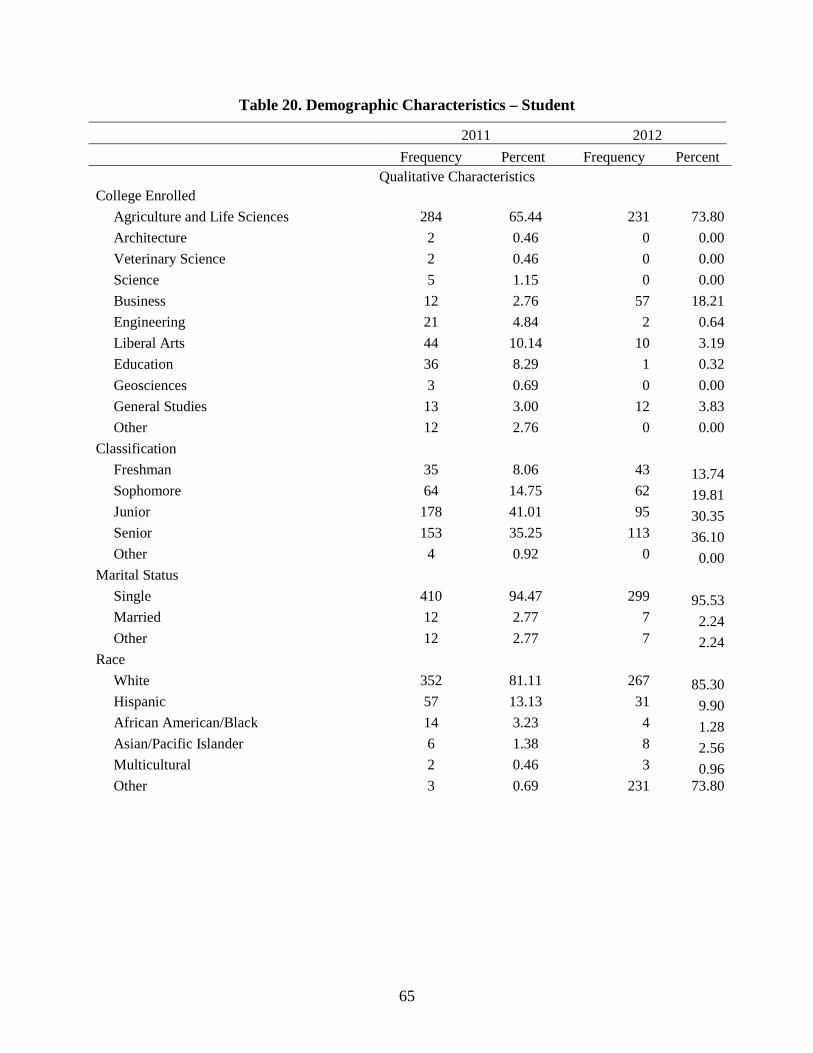
65
Table 20. Demographic Characteristics – Student
2011 2012 Frequency Percent Frequency Percent
Qualitative Characteristics College Enrolled
Agriculture and Life Sciences 284 65.44 231 73.80 Architecture 2 0.46 0 0.00 Veterinary Science 2 0.46 0 0.00 Science 5 1.15 0 0.00 Business 12 2.76 57 18.21 Engineering 21 4.84 2 0.64 Liberal Arts 44 10.14 10 3.19 Education 36 8.29 1 0.32 Geosciences 3 0.69 0 0.00 General Studies 13 3.00 12 3.83 Other 12 2.76 0 0.00
Classification Freshman 35 8.06 43 13.74 Sophomore 64 14.75 62 19.81 Junior 178 41.01 95 30.35 Senior 153 35.25 113 36.10 Other 4 0.92 0 0.00
Marital Status Single 410 94.47 299 95.53 Married 12 2.77 7 2.24 Other 12 2.77 7 2.24
Race White 352 81.11 267 85.30 Hispanic 57 13.13 31 9.90 African American/Black 14 3.23 4 1.28 Asian/Pacific Islander 6 1.38 8 2.56 Multicultural 2 0.46 3 0.96 Other 3 0.69 231 73.80
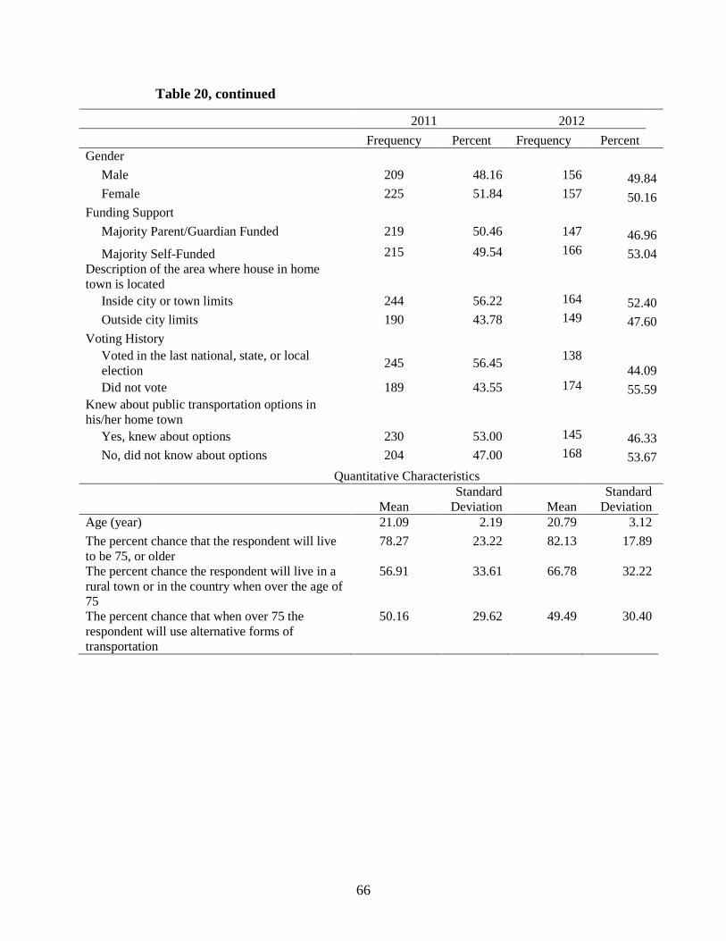
66
Table 20, continued 2011 2012 Frequency Percent Frequency Percent Gender
Male 209 48.16 156 49.84 Female 225 51.84 157 50.16
Funding Support Majority Parent/Guardian Funded 219 50.46 147 46.96 Majority Self-Funded 215 49.54 166 53.04
Description of the area where house in home town is located
Inside city or town limits 244 56.22 164 52.40 Outside city limits 190 43.78 149 47.60
Voting History Voted in the last national, state, or local election 245 56.45 138
44.09 Did not vote 189 43.55 174 55.59
Knew about public transportation options in his/her home town
Yes, knew about options 230 53.00 145 46.33 No, did not know about options 204 47.00 168 53.67
Quantitative Characteristics
Mean Standard
Deviation Mean Standard
Deviation Age (year) 21.09 2.19 20.79 3.12 The percent chance that the respondent will live to be 75, or older
78.27 23.22 82.13 17.89
The percent chance the respondent will live in a rural town or in the country when over the age of 75
56.91 33.61 66.78 32.22
The percent chance that when over 75 the respondent will use alternative forms of transportation
50.16 29.62 49.49 30.40
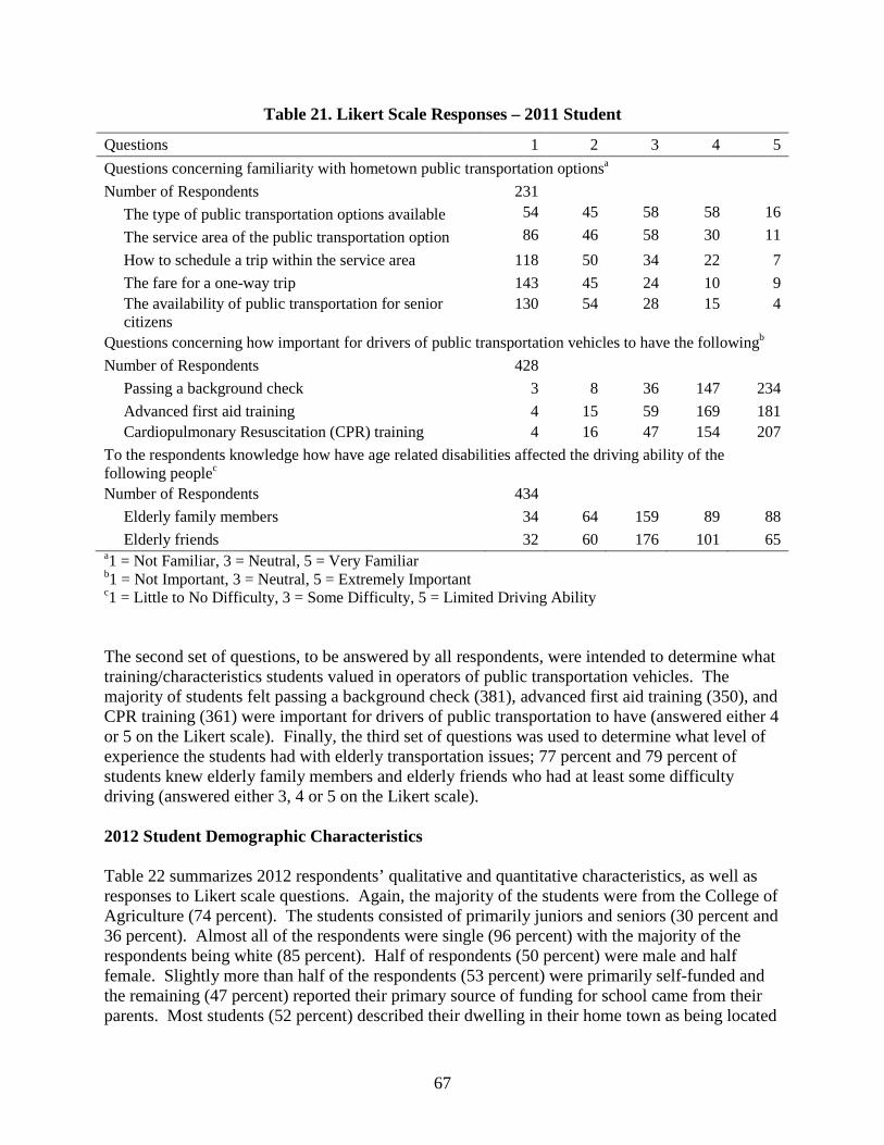
67
Table 21. Likert Scale Responses – 2011 Student
Questions 1 2 3 4 5 Questions concerning familiarity with hometown public transportation optionsa Number of Respondents 231
The type of public transportation options available 54 45 58 58 16 The service area of the public transportation option 86 46 58 30 11 How to schedule a trip within the service area 118 50 34 22 7 The fare for a one-way trip 143 45 24 10 9 The availability of public transportation for senior citizens
130 54 28 15 4
Questions concerning how important for drivers of public transportation vehicles to have the followingb Number of Respondents 428
Passing a background check 3 8 36 147 234 Advanced first aid training 4 15 59 169 181 Cardiopulmonary Resuscitation (CPR) training 4 16 47 154 207
To the respondents knowledge how have age related disabilities affected the driving ability of the following peoplec Number of Respondents 434
Elderly family members 34 64 159 89 88 Elderly friends 32 60 176 101 65
a1 = Not Familiar, 3 = Neutral, 5 = Very Familiar b1 = Not Important, 3 = Neutral, 5 = Extremely Important c1 = Little to No Difficulty, 3 = Some Difficulty, 5 = Limited Driving Ability The second set of questions, to be answered by all respondents, were intended to determine what training/characteristics students valued in operators of public transportation vehicles. The majority of students felt passing a background check (381), advanced first aid training (350), and CPR training (361) were important for drivers of public transportation to have (answered either 4 or 5 on the Likert scale). Finally, the third set of questions was used to determine what level of experience the students had with elderly transportation issues; 77 percent and 79 percent of students knew elderly family members and elderly friends who had at least some difficulty driving (answered either 3, 4 or 5 on the Likert scale). 2012 Student Demographic Characteristics Table 22 summarizes 2012 respondents’ qualitative and quantitative characteristics, as well as responses to Likert scale questions. Again, the majority of the students were from the College of Agriculture (74 percent). The students consisted of primarily juniors and seniors (30 percent and 36 percent). Almost all of the respondents were single (96 percent) with the majority of the respondents being white (85 percent). Half of respondents (50 percent) were male and half female. Slightly more than half of the respondents (53 percent) were primarily self-funded and the remaining (47 percent) reported their primary source of funding for school came from their parents. Most students (52 percent) described their dwelling in their home town as being located
68
inside the city limits than outside city limits (48 percent). Most students (82 percent) believed they would reach the age of 75, and two thirds expected that they would live in a rural area when over the age of 75. However, less than half of students (49 percent) expected that they would use alternative forms of transportation (regardless of where they lived). The Likert6 scale questions (Table 22) were utilized to judge the respondents’ knowledge and familiarity with transportation issues. The first set of questions was only to be completed by students who answered “yes” to the question, “Are there options to use public transportation in your hometown?” Of the 145 students who knew there were public transportation options in their hometown, the majority were not familiar with the various aspects of their hometown public transportation (answered either 1 or 2 on the Likert scale). One hundred five students were not familiar with the service area of the public transportation option, 120 were not familiar with how to schedule a trip, 131 were not familiar with the fare for a one-way trip, and 112 were not familiar with the availability of options for senior citizens.
The second set of questions, to be answered by all respondents, were intended to determine what training/characteristics students valued in operators of public transportation vehicles. The majority of students felt passing a background check (267), advanced first aid training (244), and CPR training (247) were important for drivers of public transportation to have (answered either 4 or 5 on the Likert scale). Finally, the third set of questions was used to determine what level of experience the students had with elderly transportation issues; 74 percent and 75 percent of students knew elderly family members and elderly friends who had at least some difficulty driving (answered either 3, 4, or 5 on the Likert scale).
6 In a Likert questionnaire item, respondents specify their level of agreement or disagreement on a symmetric agree-disagree scale for a series of statements. The scale is named after its inventor, Rensis Likert (Likert 1932).
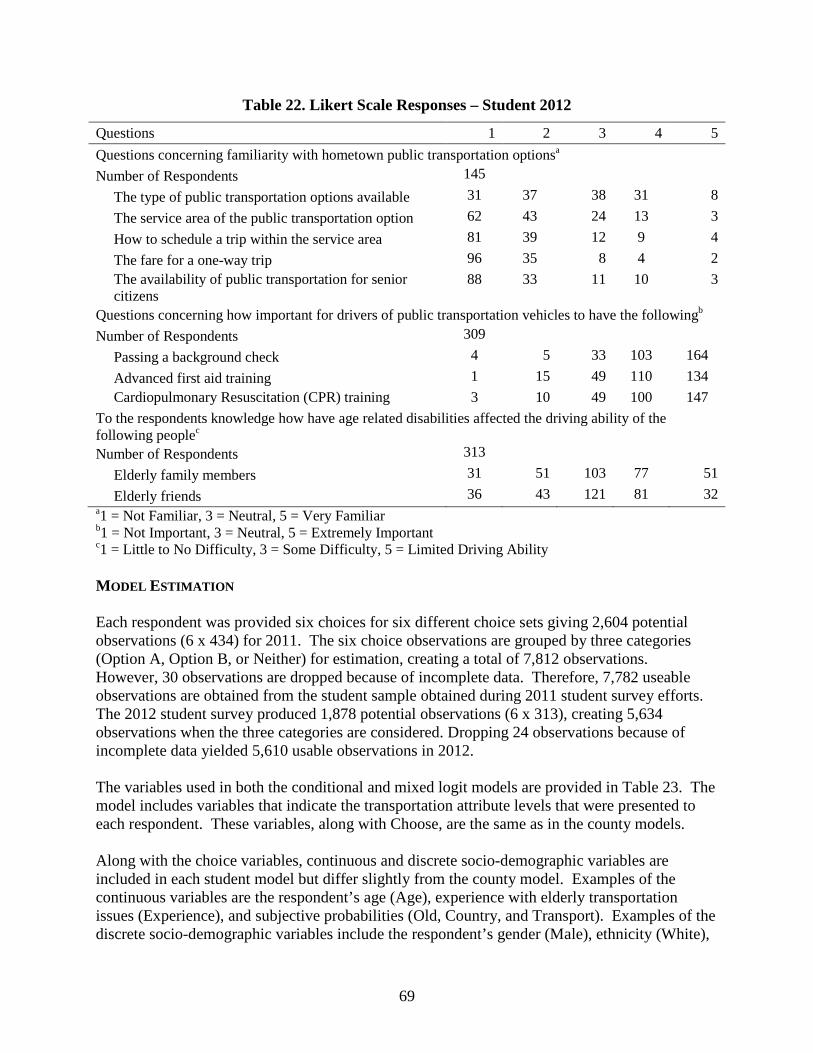
69
Table 22. Likert Scale Responses – Student 2012
Questions 1 2 3 4 5 Questions concerning familiarity with hometown public transportation optionsa Number of Respondents 145
The type of public transportation options available 31 37 38 31 8 The service area of the public transportation option 62 43 24 13 3 How to schedule a trip within the service area 81 39 12 9 4 The fare for a one-way trip 96 35 8 4 2 The availability of public transportation for senior citizens
88 33 11 10 3
Questions concerning how important for drivers of public transportation vehicles to have the followingb Number of Respondents 309
Passing a background check 4 5 33 103 164 Advanced first aid training 1 15 49 110 134 Cardiopulmonary Resuscitation (CPR) training 3 10 49 100 147
To the respondents knowledge how have age related disabilities affected the driving ability of the following peoplec Number of Respondents 313
Elderly family members 31 51 103 77 51 Elderly friends 36 43 121 81 32
a1 = Not Familiar, 3 = Neutral, 5 = Very Familiar b1 = Not Important, 3 = Neutral, 5 = Extremely Important c1 = Little to No Difficulty, 3 = Some Difficulty, 5 = Limited Driving Ability MODEL ESTIMATION Each respondent was provided six choices for six different choice sets giving 2,604 potential observations (6 x 434) for 2011. The six choice observations are grouped by three categories (Option A, Option B, or Neither) for estimation, creating a total of 7,812 observations. However, 30 observations are dropped because of incomplete data. Therefore, 7,782 useable observations are obtained from the student sample obtained during 2011 student survey efforts. The 2012 student survey produced 1,878 potential observations (6 x 313), creating 5,634 observations when the three categories are considered. Dropping 24 observations because of incomplete data yielded 5,610 usable observations in 2012. The variables used in both the conditional and mixed logit models are provided in Table 23. The model includes variables that indicate the transportation attribute levels that were presented to each respondent. These variables, along with Choose, are the same as in the county models.
Along with the choice variables, continuous and discrete socio-demographic variables are included in each student model but differ slightly from the county model. Examples of the continuous variables are the respondent’s age (Age), experience with elderly transportation issues (Experience), and subjective probabilities (Old, Country, and Transport). Examples of the discrete socio-demographic variables include the respondent’s gender (Male), ethnicity (White),
70
and voting history (Voted). An interaction variable between Choose and each socio-demographic variable is used to determine which socio-demographic variables affect the respondents’ decision to choose a transportation option.
Results from the conditional and mixed logit model estimations in 2011 and 2012 are in Table 24 and Table 27. Summary statistics for both models are in Table 28 and Table 29, and chi-squared hypothesis tests of the equality of choice variable coefficients are in Table 30 and Table 31 for 2011 and 2012, respectively. Most coefficients associated with the variables in both models are significant at the 5 percent level or less (α ≤ 0.05), implying the factors included in the model play a statistically important role in the respondents’ decision to choose a transportation option.
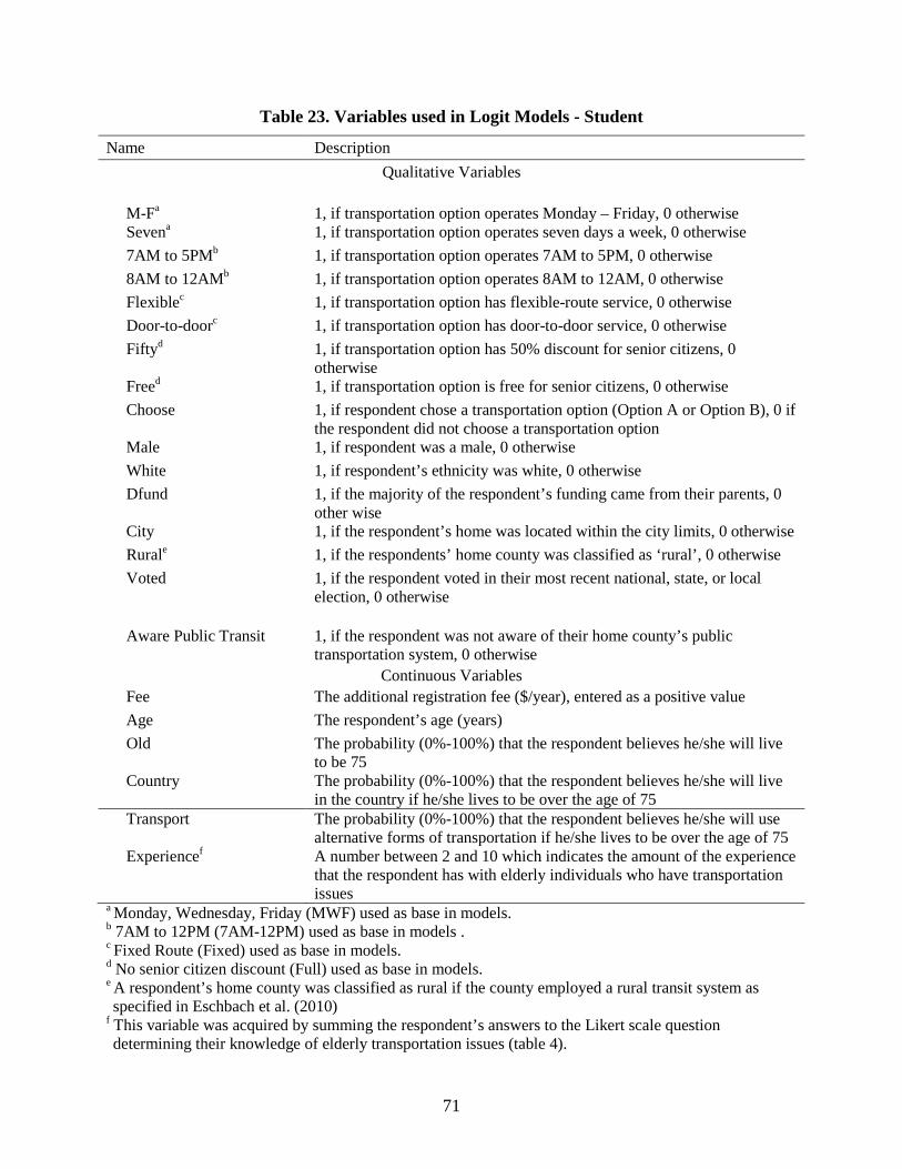
71
Table 23. Variables used in Logit Models - Student
Name Description Qualitative Variables
M-Fa
1, if transportation option operates Monday – Friday, 0 otherwise
Sevena 1, if transportation option operates seven days a week, 0 otherwise 7AM to 5PMb 1, if transportation option operates 7AM to 5PM, 0 otherwise 8AM to 12AMb 1, if transportation option operates 8AM to 12AM, 0 otherwise Flexiblec 1, if transportation option has flexible-route service, 0 otherwise Door-to-doorc 1, if transportation option has door-to-door service, 0 otherwise Fiftyd 1, if transportation option has 50% discount for senior citizens, 0
otherwise Freed 1, if transportation option is free for senior citizens, 0 otherwise Choose 1, if respondent chose a transportation option (Option A or Option B), 0 if
the respondent did not choose a transportation option Male 1, if respondent was a male, 0 otherwise White 1, if respondent’s ethnicity was white, 0 otherwise Dfund 1, if the majority of the respondent’s funding came from their parents, 0
other wise City 1, if the respondent’s home was located within the city limits, 0 otherwise Rurale 1, if the respondents’ home county was classified as ‘rural’, 0 otherwise Voted 1, if the respondent voted in their most recent national, state, or local
election, 0 otherwise Aware Public Transit
1, if the respondent was not aware of their home county’s public transportation system, 0 otherwise
Continuous Variables Fee The additional registration fee ($/year), entered as a positive value Age The respondent’s age (years) Old The probability (0%-100%) that the respondent believes he/she will live
to be 75 Country The probability (0%-100%) that the respondent believes he/she will live
in the country if he/she lives to be over the age of 75 Transport The probability (0%-100%) that the respondent believes he/she will use
alternative forms of transportation if he/she lives to be over the age of 75 Experiencef
A number between 2 and 10 which indicates the amount of the experience that the respondent has with elderly individuals who have transportation issues
a Monday, Wednesday, Friday (MWF) used as base in models. b 7AM to 12PM (7AM-12PM) used as base in models . c Fixed Route (Fixed) used as base in models. d No senior citizen discount (Full) used as base in models. e A respondent’s home county was classified as rural if the county employed a rural transit system as specified in Eschbach et al. (2010)
f This variable was acquired by summing the respondent’s answers to the Likert scale question determining their knowledge of elderly transportation issues (table 4).
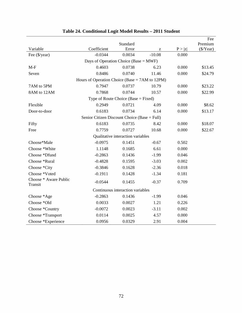
72
Table 24. Conditional Logit Model Results – 2011 Student
Variable Coefficient Standard
Error z
P > |z|
Fee Premium ($/Year)
Fee ($/year) -0.0344 0.0034 -10.08 0.000 Days of Operation Choice (Base = MWF)
M-F 0.4603 0.0738 6.23 0.000 $13.45 Seven 0.8486 0.0740 11.46 0.000 $24.79
Hours of Operation Choice (Base = 7AM to 12PM) 7AM to 5PM 0.7947 0.0737 10.79 0.000 $23.22 8AM to 12AM 0.7868 0.0744 10.57 0.000 $22.99
Type of Route Choice (Base = Fixed) Flexible 0.2949 0.0721 4.09 0.000 $8.62 Door-to-door 0.6183 0.0734 6.14 0.000 $13.17
Senior Citizen Discount Choice (Base = Full) Fifty 0.6183 0.0735 8.42 0.000 $18.07 Free 0.7759 0.0727 10.68 0.000 $22.67
Qualitative interaction variables Choose*Male -0.0975 0.1451 -0.67 0.502 Choose *White 1.1148 0.1685 6.61 0.000 Choose *Dfund -0.2863 0.1436 -1.99 0.046 Choose *Rural -0.4828 0.1595 -3.03 0.002 Choose *City -0.3846 0.1628 -2.36 0.018 Choose *Voted -0.1911 0.1428 -1.34 0.181 Choose * Aware Public Transit -0.0544 0.1455 -0.37 0.709
Continuous interaction variables Choose *Age -0.2863 0.1436 -1.99 0.046 Choose *Old 0.0033 0.0027 1.21 0.226 Choose *Country -0.0072 0.0023 -3.11 0.002 Choose *Transport 0.0114 0.0025 4.57 0.000 Choose *Experience 0.0956 0.0329 2.91 0.004
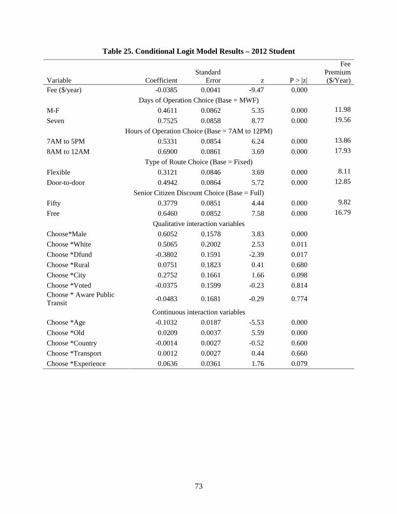
73
Table 25. Conditional Logit Model Results – 2012 Student
Variable Coefficient Standard
Error z
P > |z|
Fee Premium ($/Year)
Fee ($/year) -0.0385 0.0041 -9.47 0.000 Days of Operation Choice (Base = MWF)
M-F 0.4611 0.0862 5.35 0.000 11.98 Seven 0.7525 0.0858 8.77 0.000 19.56
Hours of Operation Choice (Base = 7AM to 12PM) 7AM to 5PM 0.5331 0.0854 6.24 0.000 13.86 8AM to 12AM 0.6900 0.0861 3.69 0.000 17.93
Type of Route Choice (Base = Fixed) Flexible 0.3121 0.0846 3.69 0.000 8.11 Door-to-door 0.4942 0.0864 5.72 0.000 12.85
Senior Citizen Discount Choice (Base = Full) Fifty 0.3779 0.0851 4.44 0.000 9.82 Free 0.6460 0.0852 7.58 0.000 16.79
Qualitative interaction variables Choose*Male 0.6052 0.1578 3.83 0.000 Choose *White 0.5065 0.2002 2.53 0.011 Choose *Dfund -0.3802 0.1591 -2.39 0.017 Choose *Rural 0.0751 0.1823 0.41 0.680 Choose *City 0.2752 0.1661 1.66 0.098 Choose *Voted -0.0375 0.1599 -0.23 0.814 Choose * Aware Public Transit -0.0483 0.1681 -0.29 0.774
Continuous interaction variables Choose *Age -0.1032 0.0187 -5.53 0.000 Choose *Old 0.0209 0.0037 5.59 0.000 Choose *Country -0.0014 0.0027 -0.52 0.600 Choose *Transport 0.0012 0.0027 0.44 0.660 Choose *Experience 0.0636 0.0361 1.76 0.079
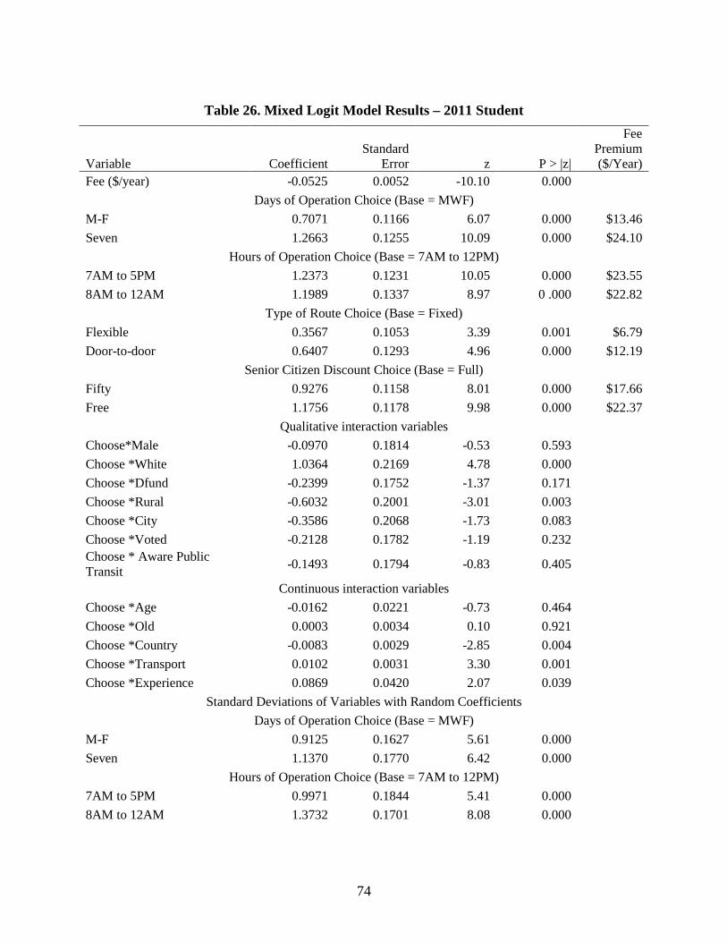
74
Table 26. Mixed Logit Model Results – 2011 Student
Variable Coefficient Standard
Error z
P > |z|
Fee Premium ($/Year)
Fee ($/year) -0.0525 0.0052 -10.10 0.000 Days of Operation Choice (Base = MWF)
M-F 0.7071 0.1166 6.07 0.000 $13.46 Seven 1.2663 0.1255 10.09 0.000 $24.10
Hours of Operation Choice (Base = 7AM to 12PM) 7AM to 5PM 1.2373 0.1231 10.05 0.000 $23.55 8AM to 12AM 1.1989 0.1337 8.97 0 .000 $22.82
Type of Route Choice (Base = Fixed) Flexible 0.3567 0.1053 3.39 0.001 $6.79 Door-to-door 0.6407 0.1293 4.96 0.000 $12.19
Senior Citizen Discount Choice (Base = Full) Fifty 0.9276 0.1158 8.01 0.000 $17.66 Free 1.1756 0.1178 9.98 0.000 $22.37
Qualitative interaction variables Choose*Male -0.0970 0.1814 -0.53 0.593 Choose *White 1.0364 0.2169 4.78 0.000 Choose *Dfund -0.2399 0.1752 -1.37 0.171 Choose *Rural -0.6032 0.2001 -3.01 0.003 Choose *City -0.3586 0.2068 -1.73 0.083 Choose *Voted -0.2128 0.1782 -1.19 0.232 Choose * Aware Public Transit -0.1493 0.1794 -0.83 0.405
Continuous interaction variables Choose *Age -0.0162 0.0221 -0.73 0.464 Choose *Old 0.0003 0.0034 0.10 0.921 Choose *Country -0.0083 0.0029 -2.85 0.004 Choose *Transport 0.0102 0.0031 3.30 0.001 Choose *Experience 0.0869 0.0420 2.07 0.039
Standard Deviations of Variables with Random Coefficients Days of Operation Choice (Base = MWF)
M-F 0.9125 0.1627 5.61 0.000 Seven 1.1370 0.1770 6.42 0.000
Hours of Operation Choice (Base = 7AM to 12PM) 7AM to 5PM 0.9971 0.1844 5.41 0.000 8AM to 12AM 1.3732 0.1701 8.08 0.000
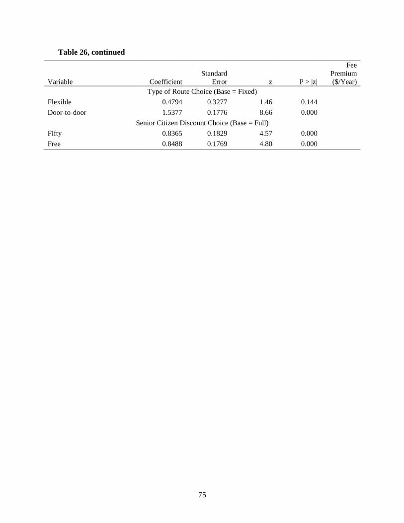
75
Table 26, continued
Variable Coefficient Standard
Error z
P > |z|
Fee Premium ($/Year)
Type of Route Choice (Base = Fixed) Flexible 0.4794 0.3277 1.46 0.144 Door-to-door 1.5377 0.1776 8.66 0.000
Senior Citizen Discount Choice (Base = Full) Fifty 0.8365 0.1829 4.57 0.000 Free 0.8488 0.1769 4.80 0.000
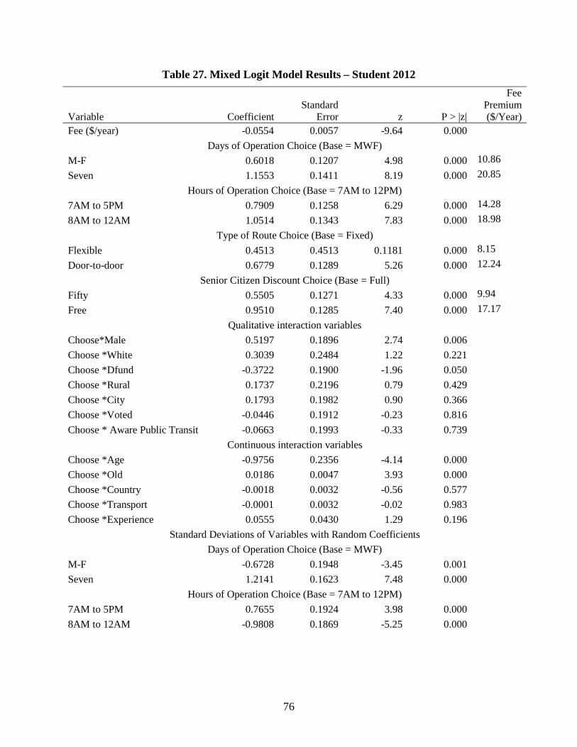
76
Table 27. Mixed Logit Model Results – Student 2012
Variable Coefficient Standard
Error z
P > |z|
Fee Premium ($/Year)
Fee ($/year) -0.0554 0.0057 -9.64 0.000 Days of Operation Choice (Base = MWF)
M-F 0.6018 0.1207 4.98 0.000 10.86 Seven 1.1553 0.1411 8.19 0.000 20.85
Hours of Operation Choice (Base = 7AM to 12PM) 7AM to 5PM 0.7909 0.1258 6.29 0.000 14.28 8AM to 12AM 1.0514 0.1343 7.83 0.000 18.98
Type of Route Choice (Base = Fixed) Flexible 0.4513 0.4513 0.1181 0.000 8.15 Door-to-door 0.6779 0.1289 5.26 0.000 12.24
Senior Citizen Discount Choice (Base = Full) Fifty 0.5505 0.1271 4.33 0.000 9.94 Free 0.9510 0.1285 7.40 0.000 17.17
Qualitative interaction variables Choose*Male 0.5197 0.1896 2.74 0.006 Choose *White 0.3039 0.2484 1.22 0.221 Choose *Dfund -0.3722 0.1900 -1.96 0.050 Choose *Rural 0.1737 0.2196 0.79 0.429 Choose *City 0.1793 0.1982 0.90 0.366 Choose *Voted -0.0446 0.1912 -0.23 0.816 Choose * Aware Public Transit -0.0663 0.1993 -0.33 0.739
Continuous interaction variables Choose *Age -0.9756 0.2356 -4.14 0.000 Choose *Old 0.0186 0.0047 3.93 0.000 Choose *Country -0.0018 0.0032 -0.56 0.577 Choose *Transport -0.0001 0.0032 -0.02 0.983 Choose *Experience 0.0555 0.0430 1.29 0.196
Standard Deviations of Variables with Random Coefficients Days of Operation Choice (Base = MWF)
M-F -0.6728 0.1948 -3.45 0.001 Seven 1.2141 0.1623 7.48 0.000
Hours of Operation Choice (Base = 7AM to 12PM) 7AM to 5PM 0.7655 0.1924 3.98 0.000 8AM to 12AM -0.9808 0.1869 -5.25 0.000
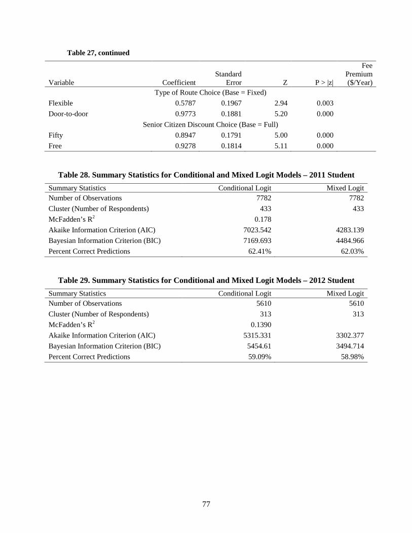
77
Table 27, continued
Variable Coefficient Standard
Error Z
P > |z|
Fee Premium ($/Year)
Type of Route Choice (Base = Fixed) Flexible 0.5787 0.1967 2.94 0.003 Door-to-door 0.9773 0.1881 5.20 0.000
Senior Citizen Discount Choice (Base = Full) Fifty 0.8947 0.1791 5.00 0.000 Free 0.9278 0.1814 5.11 0.000
Table 28. Summary Statistics for Conditional and Mixed Logit Models – 2011 Student Summary Statistics Conditional Logit Mixed Logit Number of Observations 7782 7782 Cluster (Number of Respondents) 433 433 McFadden’s R2 0.178 Akaike Information Criterion (AIC) 7023.542 4283.139 Bayesian Information Criterion (BIC) 7169.693 4484.966 Percent Correct Predictions 62.41% 62.03%
Table 29. Summary Statistics for Conditional and Mixed Logit Models – 2012 Student Summary Statistics Conditional Logit Mixed Logit Number of Observations 5610 5610 Cluster (Number of Respondents) 313 313 McFadden’s R2 0.1390 Akaike Information Criterion (AIC) 5315.331 3302.377 Bayesian Information Criterion (BIC) 5454.61 3494.714 Percent Correct Predictions 59.09% 58.98%
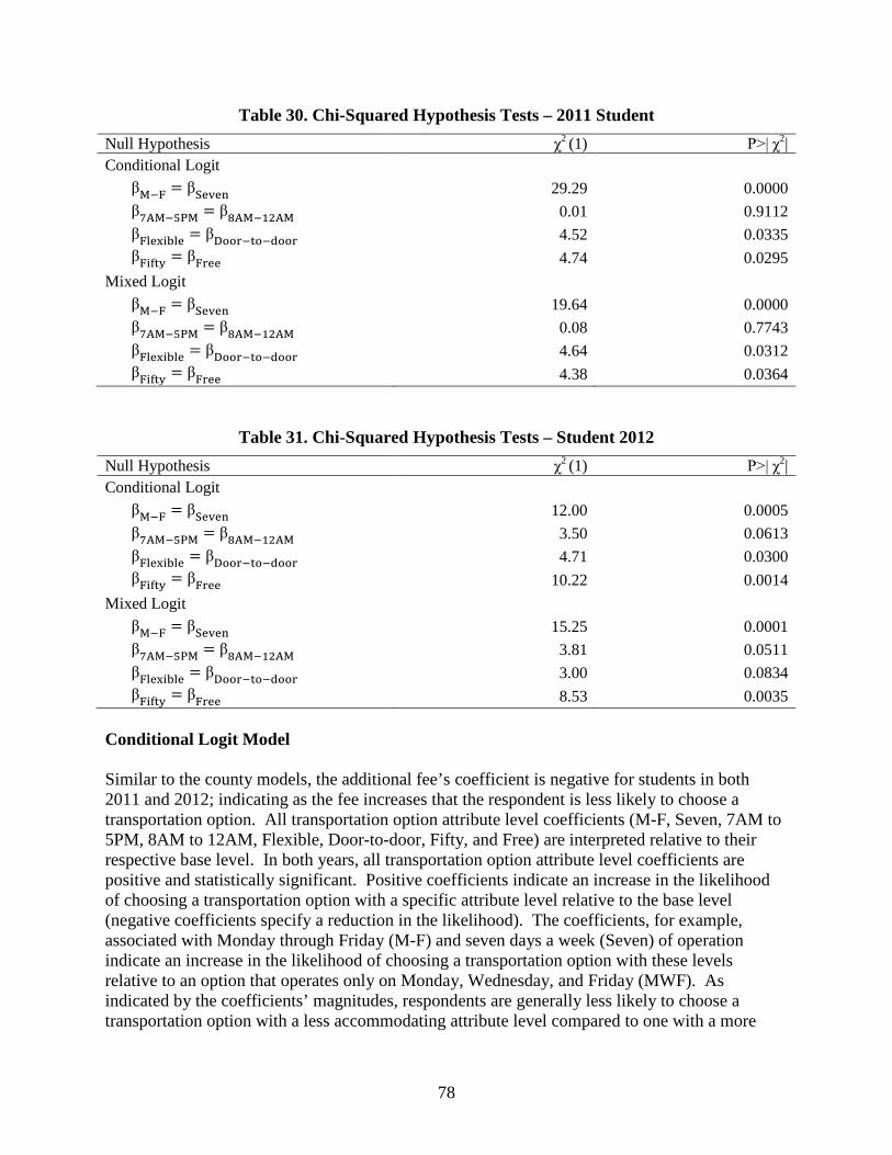
78
Table 30. Chi-Squared Hypothesis Tests – 2011 Student Null Hypothesis χ2 (1) P>| χ2| Conditional Logit
βM−F = βSeven 29.29 0.0000 β7AM−5PM = β8AM−12AM 0.01 0.9112 βFlexible = βDoor−to−door 4.52 0.0335 βFifty = βFree 4.74 0.0295
Mixed Logit βM−F = βSeven 19.64 0.0000 β7AM−5PM = β8AM−12AM 0.08 0.7743 βFlexible = βDoor−to−door 4.64 0.0312 βFifty = βFree 4.38 0.0364
Table 31. Chi-Squared Hypothesis Tests – Student 2012 Null Hypothesis χ2 (1) P>| χ2| Conditional Logit
βM−F = βSeven 12.00 0.0005 β7AM−5PM = β8AM−12AM 3.50 0.0613 βFlexible = βDoor−to−door 4.71 0.0300 βFifty = βFree 10.22 0.0014
Mixed Logit βM−F = βSeven 15.25 0.0001 β7AM−5PM = β8AM−12AM 3.81 0.0511 βFlexible = βDoor−to−door 3.00 0.0834 βFifty = βFree 8.53 0.0035
Conditional Logit Model Similar to the county models, the additional fee’s coefficient is negative for students in both 2011 and 2012; indicating as the fee increases that the respondent is less likely to choose a transportation option. All transportation option attribute level coefficients (M-F, Seven, 7AM to 5PM, 8AM to 12AM, Flexible, Door-to-door, Fifty, and Free) are interpreted relative to their respective base level. In both years, all transportation option attribute level coefficients are positive and statistically significant. Positive coefficients indicate an increase in the likelihood of choosing a transportation option with a specific attribute level relative to the base level (negative coefficients specify a reduction in the likelihood). The coefficients, for example, associated with Monday through Friday (M-F) and seven days a week (Seven) of operation indicate an increase in the likelihood of choosing a transportation option with these levels relative to an option that operates only on Monday, Wednesday, and Friday (MWF). As indicated by the coefficients’ magnitudes, respondents are generally less likely to choose a transportation option with a less accommodating attribute level compared to one with a more
79
accommodating option. The one exception being that the respondents slightly preferred a 7AM to 5PM service over an 8AM to 12AM service in 2011 although students preferred the 8AM to 12AM service in 2012 (Tables 24 and 25). Within a transportation attribute category, the null hypothesis that the coefficients of the attribute levels are the same is tested using chi-squared tests (Tables 30 and 31). Although the magnitudes of the coefficients associated with 7AM to 5PM and 8AM to 12AM services differed, the coefficients are not significantly different from each other in 2011. In 2012, the coefficients differ at the 10 percent level. Coefficients associated with the days of operation (Monday through Friday versus seven days a week), type of route (flexible versus door-to-door), and fare (50 percent discount versus free) are significantly different from each other in both years.
Besides the transportation attributes, other variables that are significant in both 2011 and 2012 are the interaction variables between Choose and the following: White, Dfund, Age, and Experience. The interaction between Choose and City is significant at the 5 percent level in 2011 but only at the 10 percent level in 2012. Interaction variables’ coefficients between Choose and White and Experience are positive. Compared to other ethnicities, a white respondent is more likely to choose a transportation option over neither. The more a respondent believes he/she will use transportation when over the age of 75 and the more experience a respondent has with elderly transportation issues, the higher the probability that the respondent will choose a transportation option over neither. The interaction between Choose and Transport was positive and significant in 2011 but was not significant in 2012. The Choose*Male interaction was positive and significant in 2012 only, suggesting that males are more likely to choose a transportation option. Similarly, the coefficient on the interaction between Choose and Old was significant and positive only in 2012; a respondent who more strongly believed he/she would reach the age of 75 was more likely to choose a transportation option. Both the interactions between Choose and Male and Old were negative and insignificant in 2011.
Interaction variables between Choose and Dfund and Age are negative. A respondent whose majority of funding for college came from their parents are less likely to choose a transportation option than a respondent who is primarily self-funded. As respondents’ age increases then he/she is less likely to choose a transportation option. The interaction of Choose and Country is negative and significant in 2011, indicating that a respondent who believes he/she will live in the country over the age of 75 is less likely to choose a transportation option. The Choose*Country interaction was not significant in 2012. In 2011, the interaction between Choose and City was negative, indicating that those respondents who lived inside the city limits are less likely to choose a transportation option. However, the Choose*City interaction is positive in 2012, although it is less significant. Similarly, the coefficient on the interaction between Choose and Rural was negative and significant at the 1 percent level in 2011, indicating that respondents who lived within a rural transit district were less likely to choose a transportation option than their metropolitan counterparts; however, in 2012 the interaction was positive but not significant.
80
Variables that were not significant in either the 2011 or 2012 student conditional model are interaction variables between Choose and Voted and Aware Public Transit. These traits (the respondent’s voting history and knowledge of public transportation in his/her home town) are not statistically significant in impacting a respondent’s decision to choose a transportation option.
Willingness-to-Pay. The coefficients for transportation option attributes are translated into WTP through additional fees on licensing a vehicle. These WTPs, in dollars per year, are given in Table 24. Positive WTPs specify the amount that respondents’ are willing to pay for a specific attribute level compared to its base level. As in the county model, all WTPs are positive meaning respondents are willing to pay more for the attributes in the model than their base level. For all attributes, except hours of operation, respondents are willing to pay the least for the less accommodating level of an attribute, and more for the most accommodating levels. The conditional logit model shows the 2011 students’ mean annual willingness-to-pay is (relative to the base level):
1) $25 more for a seven days a week service and $13 more for a Monday through Friday
service than a Monday, Wednesday, Friday service; 2) $23 more for an 8AM to 12 midnight service or a 7AM to 5PM service than a 7AM to
12AM service; 3) $13 more for a door-to-door route and $9 more for a flexible route than a fixed route;
and 4) $23 more for an option with free fare for senior citizens and $18 more for an option
that gives a 50 percent discount for senior citizens than an option that gives no discount.
The conditional logit model shows the 2012 students’ mean annual willingness-to-pay is (relative to the base level):
1) $20 more for a seven days a week service and $12 more for a Monday through Friday
service than a Monday, Wednesday, Friday service; 2) $18 more for an 8AM to 12 midnight service or $14 more for a 7AM to 5PM service
than a 7AM to 12AM service; 3) $13 more for a door-to-door route and $8 more for a flexible route than a fixed route;
and 4) $17 more for an option with free fare for senior citizens and $108 more for an option
that gives a 50 percent discount for senior citizens than an option that gives no discount.
Mixed Logit Model As in the county model, results from the mixed logit model are similar to the conditional logit model in terms of the transportation attributes. The additional fee’s coefficient is statistically significant and negative; whereas, all transportation option attribute levels are statistically significant and positive in both 2011 and 2012. The coefficient inferences remain the same. Including these attributes increases the probability that a respondent will choose a transportation
81
option over another. Similar to the conditional model, coefficients for transportation attributes, except for hours, are statistically different from each other (Tables 30 and 31). The significance of interaction variables changes drastically from 2011 to 2012. Interactions between Choose and City, Voted, and Aware Public Transit are never significant. Interactions with Voted and Aware Public Transit are also never significant in the conditional models. Interactions between Choose and Male, Rural, County, Transport, and Experience are significant at the 5 percent level in 2011. Interactions between Choose and Male, Dfund, Age, and Old are significant in 2012. Among the interactions that are significant in one period, coefficients on four interactions (between Choose and Male, Rural, City, and Transport) changed signs between the two years. The Male, Rural, and City interactions also changed signs in the conditional models. Among variables that were significant in one year and did not change signs, interactions between Choose and White, Old, and Experience are positive in the mixed logit models as they were for the conditional models. Interactions between Choose and Dfund, Age and Country are negative in both the mixed and conditional logit models. Willingness-to-Pay. As in the conditional model, the coefficients for transportation option attributes in the mixed model are translated into yearly WTP (Tables 26 and 27). The resulting WTPs are similar to those calculated in the conditional logit model. The 2011 student population is willing to annually pay:
1) $24 more for a seven days a week service and $13 more for a Monday through Friday
service than a Monday, Wednesday, Friday service; 2) $23 more for an 8AM to 12 midnight service and $24 more for a 7AM to 5PM service
than a 7AM to 12AM service; 3) $12 more for a door-to-door route and $7 more for a flexible route than a fixed route;
and 4) $22 more for an option with free fare for senior citizens and $18 more for an option
that gives a 50 percent discount for senior citizens than an option that gives no discount.
As explained in the county mixed logit model results, one advantage of the mixed logit model is the percentages of the student population and sample (see Methodology for explanation of population versus sample) that prefer the attribute over the base attribute (indicated by a positive WTP) can be calculated:
1) 78 percent of the student population and 94 percent of the student sample prefer
Monday through Friday service over Monday, Wednesday, Friday service; 2) 87 percent of the student population and 98 percent of the student sample prefer seven
days a week service over Monday, Wednesday, Friday service; 3) 89 percent of the student population and 99 percent of the student sample prefer 7AM
to 5PM service over 7AM to 12PM service; 4) 81 percent of the student population and 93 percent of the student sample prefer 8AM
to 12AM service over 7AM to 12PM service;
82
5) 77 percent of the student population and 98 percent of the student sample prefer a flexible route over a fixed route;
6) 66 percent of the student population and 76 percent of the student sample prefer a door-to-door route over a fixed route;
7) 87 percent of the student population and 99 percent of the student sample prefer a 50 percent discount over no discount for senior citizens; and
8) 92 percent of the student population and 100 percent of the student sample prefer free fare over no discount for senior citizens.
The 2012 student population is willing to annually pay:
1) $21 more for a seven days a week service and $11 more for a Monday through Friday
service than a Monday, Wednesday, Friday service; 2) $19 more for an 8AM to 12 midnight service and $14 more for a 7AM to 5PM service
than a 7AM to 12AM service; 3) $12 more for a door-to-door route and $8 more for a flexible route than a fixed route;
and 4) $17 more for an option with free fare for senior citizens and $10 more for an option
that gives a 50 percent discount for senior citizens than an option that gives no discount.
As explained in the county mixed logit model results, one advantage of the mixed logit model is the percentages of the student population and sample (see Methodology for explanation of population versus sample) that prefer the attribute over the base attribute (indicated by a positive WTP) can be calculated:
1) 81 percent of the student population and 97 percent of the student sample prefer
Monday through Friday service over Monday, Wednesday, Friday service; 2) 83 percent of the student population and 88 percent of the student sample prefer seven
days a week service over Monday, Wednesday, Friday service; 3) 85 percent of the student population and 91 percent of the student sample prefer 7AM
to 5PM service over 7AM to 12PM service; 4) 86 percent of the student population and 97 percent of the student sample prefer 8AM
to 12AM service over 7AM to 12PM service; 5) 78 percent of the student population and 98 percent of the student sample prefer a
flexible route over a fixed route; 6) 76 percent of the student population and 99 percent of the student sample prefer a
door-to-door route over a fixed route; 7) 73 percent of the student population and 94 percent of the student sample prefer a
50 percent discount over no discount for senior citizens; and 8) 85 percent of the student population and 98 percent of the student sample prefer free
fare over no discount for senior citizens.
83
DIFFERENCES BETWEEN THE CONDITIONAL LOGIT AND MIXED LOGIT MODELS The estimated variable coefficients are similar between both models. In terms of significance, the largest difference between the conditional and mixed logit models is the coefficient for the interaction variable between Choose and Age. In the conditional model, this coefficient is significant at the 5 percent level, but in the mixed logit model its significance is at the 46 percent level. There are two notable differences between the two models for the WTP of route attribute levels. In the mixed logit model, students are willing to pay almost 27 percent less for a flexible route service and 8 percent less for a door-to-door service than in the conditional model. Both models have approximately the same correct predictions (62 percent in 2011 and 59 percent in 2012). The standard deviations of the variables with random coefficients in the mixed logit model are highly significant (except that the coefficient for a flexible route is significant at only the 15 percent level in 2011). Significance of the standard errors indicates these coefficients vary within the population (Table 26 and Table 27). Based on these tests, it is concluded that the mixed logit model is statistically preferred to the conditional logit model.
CHAPTER 7. FINDINGS – POPULATION AND INDIVIDUAL WILLINGNESS-TO-PAY COMPARISONS
Given the previously defined chi-squared tests, similarities between the WTP between the three counties is expected. All mean WTP are positive in both the conditional and mixed logit models, indicating a positive WTP for the attributes that are more flexible than the base attributes. For most attribute categories, the calculated WTP increases for the more flexible option over the least flexible. CONDITIONAL LOGIT WTP COMPARISONS Comparisons of each population’s WTP and the standard deviation of its WTP calculated from the conditional logit estimation are found in Table 32 and Figure 4. Overall, the student population is willing to pay more for all transportation option attribute levels, especially the 2011 cohort of surveyed students. Each county has at least one attribute for which it is willing to pay more than the other two counties and one attribute that it values less than the other two counties. The standard deviations for the attributes range from $2 to $3.23. Neither students nor any single county consistently has the highest standard deviation in WTP.
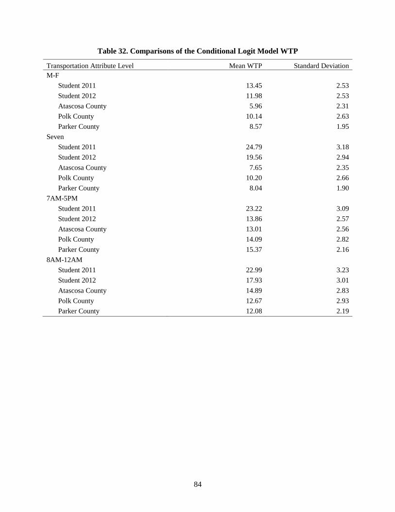
84
Table 32. Comparisons of the Conditional Logit Model WTP
Transportation Attribute Level Mean WTP Standard Deviation M-F
Student 2011 13.45 2.53 Student 2012 11.98 2.53 Atascosa County 5.96 2.31 Polk County 10.14 2.63 Parker County 8.57 1.95
Seven Student 2011 24.79 3.18 Student 2012 19.56 2.94 Atascosa County 7.65 2.35 Polk County 10.20 2.66 Parker County 8.04 1.90
7AM-5PM Student 2011 23.22 3.09 Student 2012 13.86 2.57 Atascosa County 13.01 2.56 Polk County 14.09 2.82 Parker County 15.37 2.16
8AM-12AM Student 2011 22.99 3.23 Student 2012 17.93 3.01 Atascosa County 14.89 2.83 Polk County 12.67 2.93 Parker County 12.08 2.19
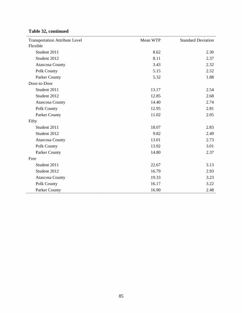
85
Table 32, continued
Transportation Attribute Level Mean WTP Standard Deviation Flexible
Student 2011 8.62 2.30 Student 2012 8.11 2.37 Atascosa County 3.43 2.32 Polk County 5.15 2.52 Parker County 5.32 1.88
Door-to-Door Student 2011 13.17 2.54 Student 2012 12.85 2.68 Atascosa County 14.40 2.74 Polk County 12.95 2.81 Parker County 11.02 2.05
Fifty Student 2011 18.07 2.83 Student 2012 9.82 2.49 Atascosa County 13.01 2.73 Polk County 13.92 3.01 Parker County 14.80 2.37
Free Student 2011 22.67 3.13 Student 2012 16.79 2.93 Atascosa County 19.33 3.23 Polk County 16.17 3.22 Parker County 16.90 2.48
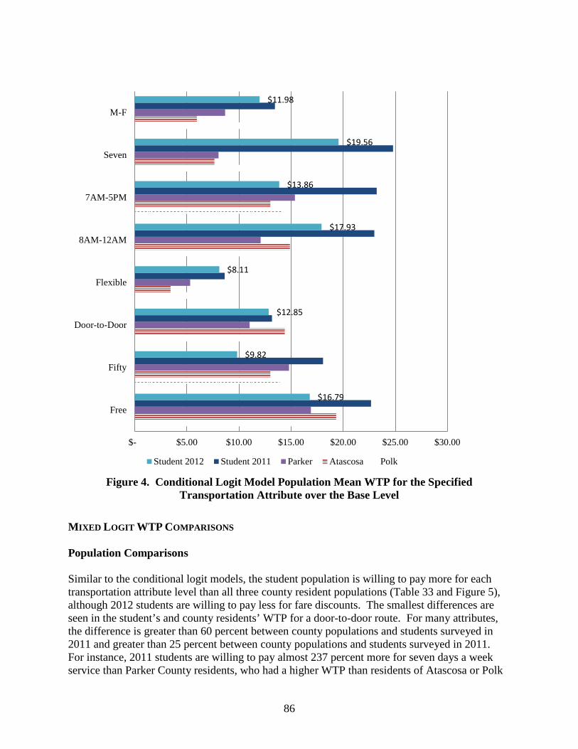
86
Figure 4. Conditional Logit Model Population Mean WTP for the Specified
Transportation Attribute over the Base Level MIXED LOGIT WTP COMPARISONS Population Comparisons Similar to the conditional logit models, the student population is willing to pay more for each transportation attribute level than all three county resident populations (Table 33 and Figure 5), although 2012 students are willing to pay less for fare discounts. The smallest differences are seen in the student’s and county residents’ WTP for a door-to-door route. For many attributes, the difference is greater than 60 percent between county populations and students surveyed in 2011 and greater than 25 percent between county populations and students surveyed in 2011. For instance, 2011 students are willing to pay almost 237 percent more for seven days a week service than Parker County residents, who had a higher WTP than residents of Atascosa or Polk
$16.79
$9.82
$12.85
$8.11
$17.93
$13.86
$19.56
$11.98
$- $5.00 $10.00 $15.00 $20.00 $25.00 $30.00
Free
Fifty
Door-to-Door
Flexible
8AM-12AM
7AM-5PM
Seven
M-F
Student 2012 Student 2011 Parker Atascosa Polk
87
Counties. Differences in WTP among the three counties are generally much smaller than differences between students and county residents. As mentioned in the previous two chapters, one benefit to using the mixed logit model is that a percentage of the population who prefer a specific attribute can be calculated. A higher percentage of the student population prefers most attribute levels over the base than the two county resident populations (Figure 6). More Polk County residents prefer a 50 percent discount and door-to-door service than students or Atascosa County residents. Sample Comparisons Another advantage to employing the mixed logit model is that individual coefficients for the variables with random coefficients are calculated. These individual level coefficients are used to calculate individual WTP. Using the mean and standard deviation of the sample’s individual WTPs, the normal distribution is used (each variable is assumed to be normally distributed) to create a probability density function to represent each sample’s WTP (Figure 7). The WTP distribution of the students, Atascosa and Polk County residents are represented in each figure, allowing the distributions to be easily compared. Days of Operation. The Atascosa County sample has the highest variance in WTP for Monday through Friday service, followed by the 2001 student then the Polk County sample. Parker County has the lowest variance. More Atascosa residents prefer the base level (Monday, Wednesday, Friday service) over Monday through Friday service than either the students or other county residents, as given by negative WTPs. Students, following the population results, had a higher mean WTP for this level, followed by Parker County residents. Similar to the population results, the students have the highest mean WTP for seven days a week of operation. The three county samples had very similar WTPs. The students have a notably larger variance than the county residents. Some students are willing to pay up to $60 for seven days a week service.
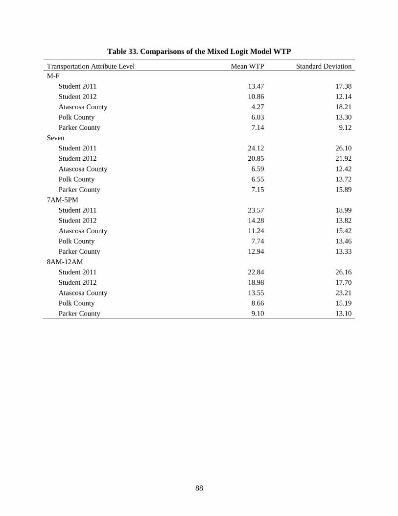
88
Table 33. Comparisons of the Mixed Logit Model WTP
Transportation Attribute Level Mean WTP Standard Deviation M-F
Student 2011 13.47 17.38 Student 2012 10.86 12.14 Atascosa County 4.27 18.21 Polk County 6.03 13.30 Parker County 7.14 9.12
Seven Student 2011 24.12 26.10 Student 2012 20.85 21.92 Atascosa County 6.59 12.42 Polk County 6.55 13.72 Parker County 7.15 15.89
7AM-5PM Student 2011 23.57 18.99 Student 2012 14.28 13.82 Atascosa County 11.24 15.42 Polk County 7.74 13.46 Parker County 12.94 13.33
8AM-12AM Student 2011 22.84 26.16 Student 2012 18.98 17.70 Atascosa County 13.55 23.21 Polk County 8.66 15.19 Parker County 9.10 13.10
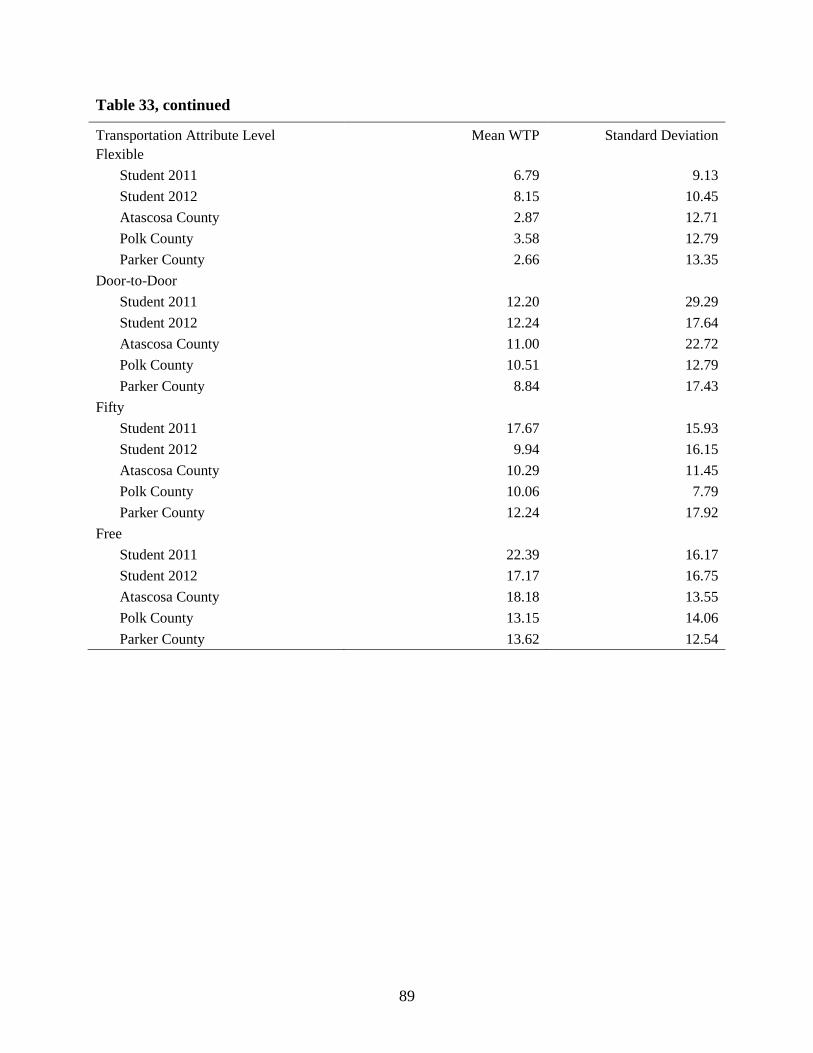
89
Table 33, continued
Transportation Attribute Level Mean WTP Standard Deviation Flexible
Student 2011 6.79 9.13 Student 2012 8.15 10.45 Atascosa County 2.87 12.71 Polk County 3.58 12.79 Parker County 2.66 13.35
Door-to-Door Student 2011 12.20 29.29 Student 2012 12.24 17.64 Atascosa County 11.00 22.72 Polk County 10.51 12.79 Parker County 8.84 17.43
Fifty Student 2011 17.67 15.93 Student 2012 9.94 16.15 Atascosa County 10.29 11.45 Polk County 10.06 7.79 Parker County 12.24 17.92
Free Student 2011 22.39 16.17 Student 2012 17.17 16.75 Atascosa County 18.18 13.55 Polk County 13.15 14.06 Parker County 13.62 12.54
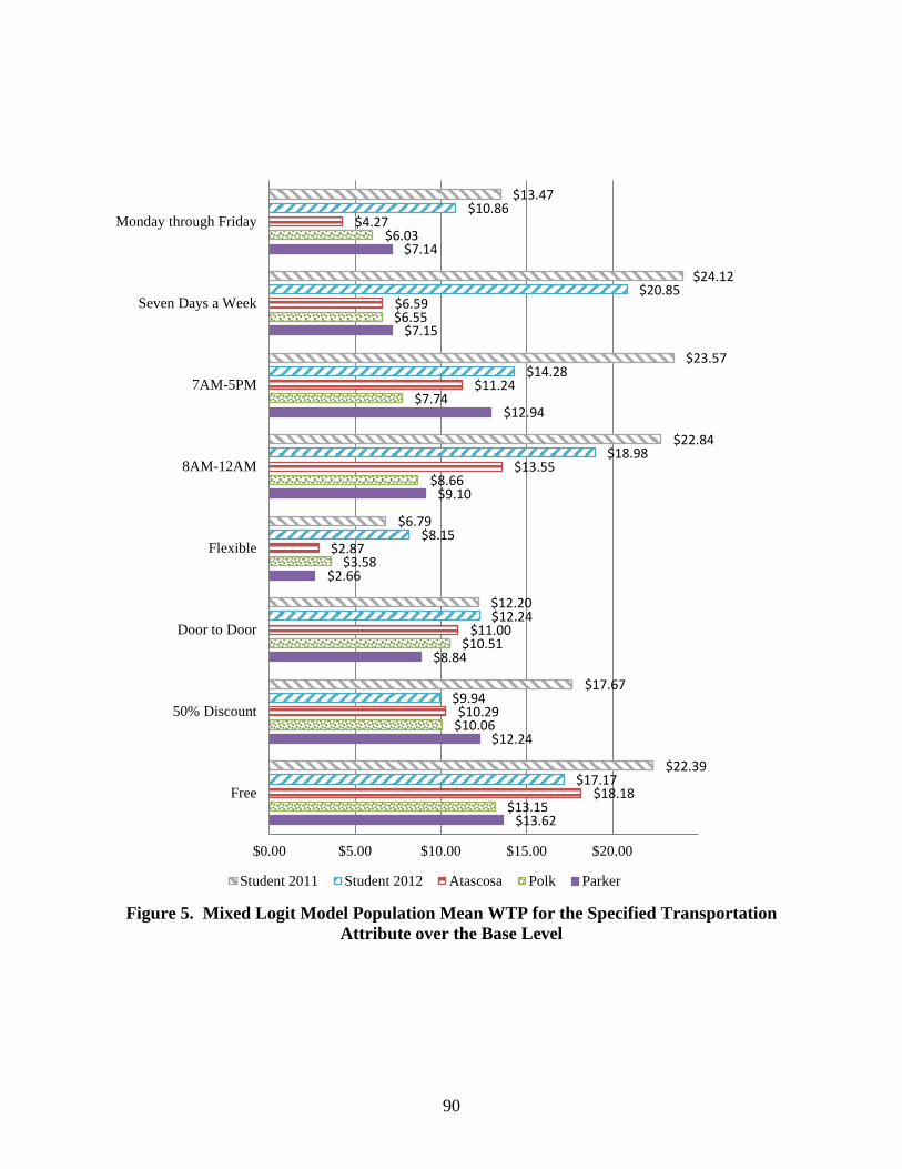
90
Figure 5. Mixed Logit Model Population Mean WTP for the Specified Transportation
Attribute over the Base Level
$13.62
$12.24
$8.84
$2.66
$9.10
$12.94
$7.15
$7.14
$13.15
$10.06
$10.51
$3.58
$8.66
$7.74
$6.55
$6.03
$18.18
$10.29
$11.00
$2.87
$13.55
$11.24
$6.59
$4.27
$17.17
$9.94
$12.24
$8.15
$18.98
$14.28
$20.85
$10.86
$22.39
$17.67
$12.20
$6.79
$22.84
$23.57
$24.12
$13.47
$0.00 $5.00 $10.00 $15.00 $20.00
Free
50% Discount
Door to Door
Flexible
8AM-12AM
7AM-5PM
Seven Days a Week
Monday through Friday
Student 2011 Student 2012 Atascosa Polk Parker
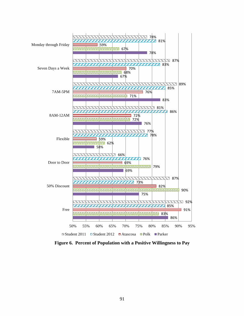
91
Figure 6. Percent of Population with a Positive Willingness to Pay
86%
75%
69%
58%
76%
83%
67%
78%
83%
90%
79%
62%
72%
71%
68%
67%
91%
82%
69%
59%
72%
76%
70%
59%
85%
73%
76%
78%
86%
85%
83%
81%
92%
87%
66%
77%
81%
89%
87%
78%
50% 55% 60% 65% 70% 75% 80% 85% 90% 95%
Free
50% Discount
Door to Door
Flexible
8AM-12AM
7AM-5PM
Seven Days a Week
Monday through Friday
Student 2011 Student 2012 Atascosa Polk Parker
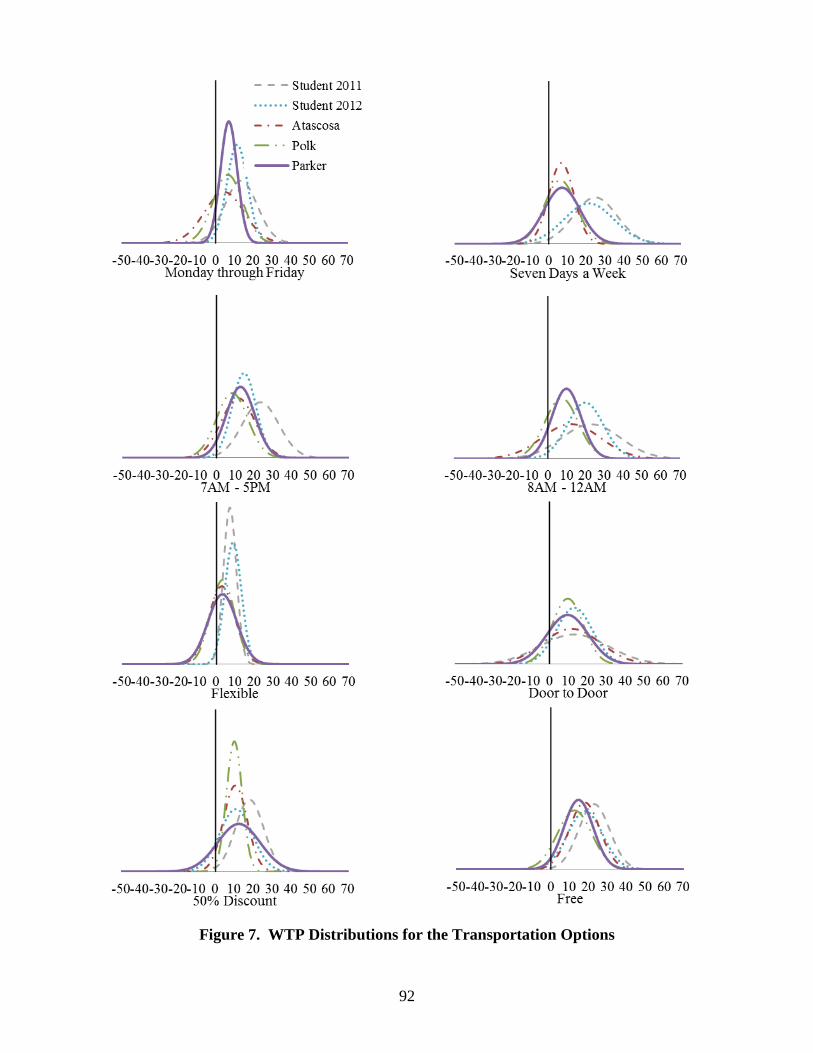
92
Figure 7. WTP Distributions for the Transportation Options
93
Hours of Operation. Following the population results, students had the highest mean WTP for 7AM to 5PM service, followed by Parker, Atascosa, and then Polk County residents (Figure 7). The variances of each sample’s WTP are similar. The means of the 8AM to 12AM service distributions follow the same pattern as the population WTP; students are willing to pay the most followed by Parker, Atascosa, and Polk residents (Figure 7). The Atascosa County resident and 2011 student WTP distribution variances are similar; the 2011 student distribution looks like the Atascosa distribution shifted to the right. The Parker and Polk resident and the 2012 student WTP distribution has a much smaller variance.
Type of Route. The variance of the students’ WTP for a flexible route is notably smaller than the counties’ variances (Figure 7). The county variances are larger with a large proportion of both WTP distributions falling into negative values; more of the county residents prefer a fixed to a flexible route. Very few of the students’ WTP’s fall into the negative range; this shows an almost unanimous preference for the flexible over the fixed route. Following the population means, the students’ sample distribution mean WTP is larger than the counties’ mean WTPs. The county distributions are similar. The distribution means of the samples are very similar for the WTP for a door-to-door route (Figure 7). The student mean WTP is slightly larger than the three counties. Atascosa County’s mean WTP is slightly larger than the Polk County mean WTP. The variances of the 2011 student and Atascosa County WTP distributions are similar. The Parker and Polk County and 2012 student WTP distributions have a smaller variance. Senior Citizen Transportation Fare Discount. Again, the sample distribution mean WTP for a 50 percent fare discount for senior citizens follow the population distribution means; 2011 students have a larger mean WTP than the counties or 2012 students, whose mean WTP are similar (Figure 7). The majority of all distributions fall in a positive WTP range indicating the students and residents prefer a 50 percent discount over senior citizens not receiving a fare discount. As with the 50 percent discount distributions, the greater part of the full fare discount WTP distributions are positive (Figure 7). The variance of each sample’s WTP is similar, but the mean WTPs differ among the samples.
Attribute Level WTP Distribution Comparisons. The null hypothesis that the WTP distributions of two population samples are equal is tested using a two-sample Wilcoxon-Mann-Whitney rank-sum test (Table 34). Of the 24 pairwise comparisons among the three counties, 14 of the null hypothesis (58 percent of the comparisons) are failed to reject at the 5 percent level. For the eight comparisons between the two student samples, only one is not rejected (13 percent of the comparisons). Door-to-door WTP distributions appear to be similar between the two student populations. Five of the 48 comparisons (10 percent) among the student and county samples are rejected at the 5 percent level. Of these five comparisons, Atascosa County is involved in four and student 2012 in four. The five distributions are: student 2011 versus Atascosa and student 2012 and Atascosa for door to door; student 2012 versus Atascosa and student 2012 versus Polk for 50 percent discount; and Student versus Atascosa for Free.
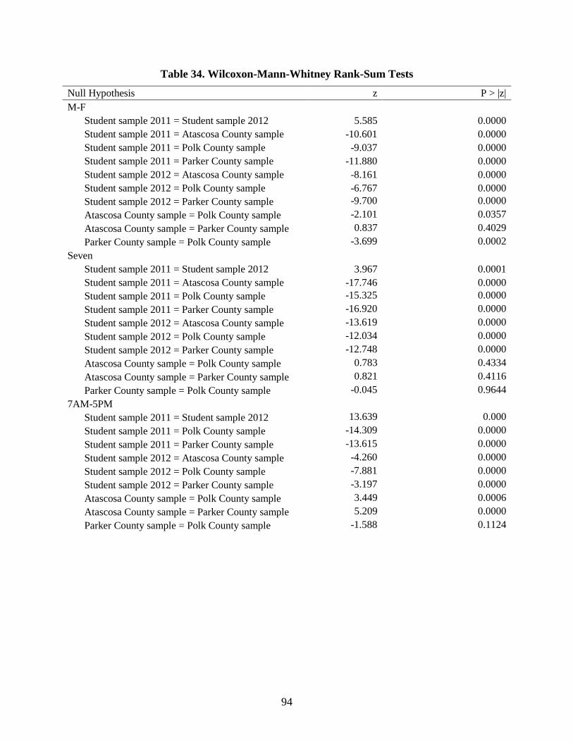
94
Table 34. Wilcoxon-Mann-Whitney Rank-Sum Tests
Null Hypothesis z P > |z| M-F
Student sample 2011 = Student sample 2012 5.585 0.0000 Student sample 2011 = Atascosa County sample -10.601 0.0000 Student sample 2011 = Polk County sample -9.037 0.0000 Student sample 2011 = Parker County sample -11.880 0.0000 Student sample 2012 = Atascosa County sample -8.161 0.0000 Student sample 2012 = Polk County sample -6.767 0.0000 Student sample 2012 = Parker County sample -9.700 0.0000 Atascosa County sample = Polk County sample -2.101 0.0357 Atascosa County sample = Parker County sample 0.837 0.4029 Parker County sample = Polk County sample -3.699 0.0002
Seven Student sample 2011 = Student sample 2012 3.967 0.0001 Student sample 2011 = Atascosa County sample -17.746 0.0000 Student sample 2011 = Polk County sample -15.325 0.0000 Student sample 2011 = Parker County sample -16.920 0.0000 Student sample 2012 = Atascosa County sample -13.619 0.0000 Student sample 2012 = Polk County sample -12.034 0.0000 Student sample 2012 = Parker County sample -12.748 0.0000 Atascosa County sample = Polk County sample 0.783 0.4334 Atascosa County sample = Parker County sample 0.821 0.4116 Parker County sample = Polk County sample -0.045 0.9644
7AM-5PM Student sample 2011 = Student sample 2012 13.639 0.000 Student sample 2011 = Polk County sample -14.309 0.0000 Student sample 2011 = Parker County sample -13.615 0.0000 Student sample 2012 = Atascosa County sample -4.260 0.0000 Student sample 2012 = Polk County sample -7.881 0.0000 Student sample 2012 = Parker County sample -3.197 0.0000 Atascosa County sample = Polk County sample 3.449 0.0006 Atascosa County sample = Parker County sample 5.209 0.0000 Parker County sample = Polk County sample -1.588 0.1124
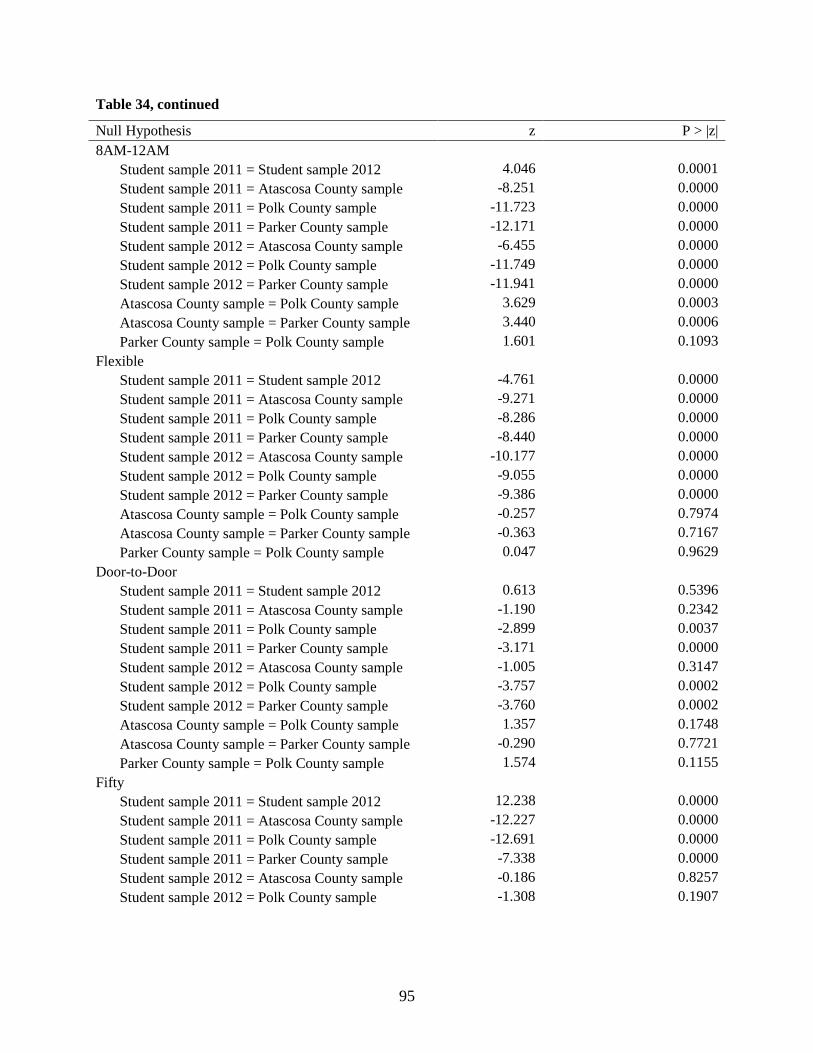
95
Table 34, continued Null Hypothesis z P > |z| 8AM-12AM
Student sample 2011 = Student sample 2012 4.046 0.0001 Student sample 2011 = Atascosa County sample -8.251 0.0000 Student sample 2011 = Polk County sample -11.723 0.0000 Student sample 2011 = Parker County sample -12.171 0.0000 Student sample 2012 = Atascosa County sample -6.455 0.0000 Student sample 2012 = Polk County sample -11.749 0.0000 Student sample 2012 = Parker County sample -11.941 0.0000 Atascosa County sample = Polk County sample 3.629 0.0003 Atascosa County sample = Parker County sample 3.440 0.0006 Parker County sample = Polk County sample 1.601 0.1093
Flexible Student sample 2011 = Student sample 2012 -4.761 0.0000 Student sample 2011 = Atascosa County sample -9.271 0.0000 Student sample 2011 = Polk County sample -8.286 0.0000 Student sample 2011 = Parker County sample -8.440 0.0000 Student sample 2012 = Atascosa County sample -10.177 0.0000 Student sample 2012 = Polk County sample -9.055 0.0000 Student sample 2012 = Parker County sample -9.386 0.0000 Atascosa County sample = Polk County sample -0.257 0.7974 Atascosa County sample = Parker County sample -0.363 0.7167 Parker County sample = Polk County sample 0.047 0.9629
Door-to-Door Student sample 2011 = Student sample 2012 0.613 0.5396 Student sample 2011 = Atascosa County sample -1.190 0.2342 Student sample 2011 = Polk County sample -2.899 0.0037 Student sample 2011 = Parker County sample -3.171 0.0000 Student sample 2012 = Atascosa County sample -1.005 0.3147 Student sample 2012 = Polk County sample -3.757 0.0002 Student sample 2012 = Parker County sample -3.760 0.0002 Atascosa County sample = Polk County sample 1.357 0.1748 Atascosa County sample = Parker County sample -0.290 0.7721 Parker County sample = Polk County sample 1.574 0.1155
Fifty Student sample 2011 = Student sample 2012 12.238 0.0000 Student sample 2011 = Atascosa County sample -12.227 0.0000 Student sample 2011 = Polk County sample -12.691 0.0000 Student sample 2011 = Parker County sample -7.338 0.0000 Student sample 2012 = Atascosa County sample -0.186 0.8257 Student sample 2012 = Polk County sample -1.308 0.1907
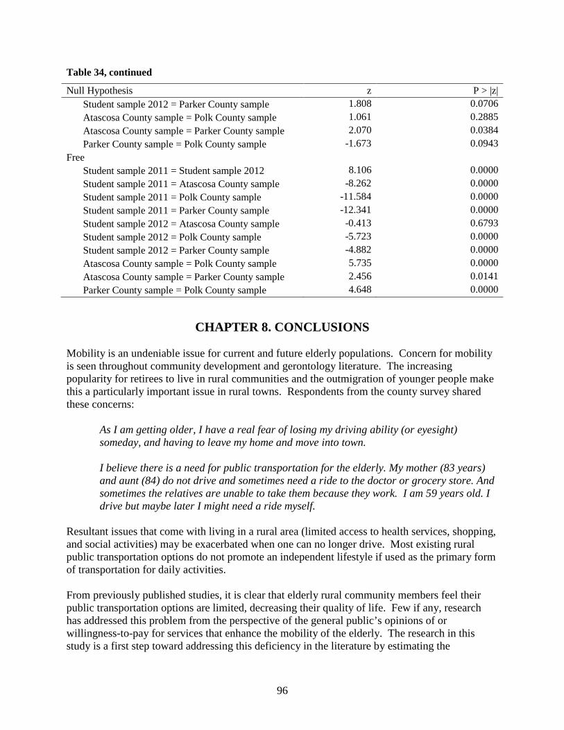
96
Table 34, continued Null Hypothesis z P > |z|
Student sample 2012 = Parker County sample 1.808 0.0706 Atascosa County sample = Polk County sample 1.061 0.2885 Atascosa County sample = Parker County sample 2.070 0.0384 Parker County sample = Polk County sample -1.673 0.0943
Free Student sample 2011 = Student sample 2012 8.106 0.0000 Student sample 2011 = Atascosa County sample -8.262 0.0000 Student sample 2011 = Polk County sample -11.584 0.0000 Student sample 2011 = Parker County sample -12.341 0.0000 Student sample 2012 = Atascosa County sample -0.413 0.6793 Student sample 2012 = Polk County sample -5.723 0.0000 Student sample 2012 = Parker County sample -4.882 0.0000 Atascosa County sample = Polk County sample 5.735 0.0000 Atascosa County sample = Parker County sample 2.456 0.0141 Parker County sample = Polk County sample 4.648 0.0000
CHAPTER 8. CONCLUSIONS
Mobility is an undeniable issue for current and future elderly populations. Concern for mobility is seen throughout community development and gerontology literature. The increasing popularity for retirees to live in rural communities and the outmigration of younger people make this a particularly important issue in rural towns. Respondents from the county survey shared these concerns:
As I am getting older, I have a real fear of losing my driving ability (or eyesight) someday, and having to leave my home and move into town. I believe there is a need for public transportation for the elderly. My mother (83 years) and aunt (84) do not drive and sometimes need a ride to the doctor or grocery store. And sometimes the relatives are unable to take them because they work. I am 59 years old. I drive but maybe later I might need a ride myself.
Resultant issues that come with living in a rural area (limited access to health services, shopping, and social activities) may be exacerbated when one can no longer drive. Most existing rural public transportation options do not promote an independent lifestyle if used as the primary form of transportation for daily activities. From previously published studies, it is clear that elderly rural community members feel their public transportation options are limited, decreasing their quality of life. Few if any, research has addressed this problem from the perspective of the general public’s opinions of or willingness-to-pay for services that enhance the mobility of the elderly. The research in this study is a first step toward addressing this deficiency in the literature by estimating the
97
willingness-to-pay for transportation options that support the rural elderly. An updated rural transportation system would most likely need to be funded by taxpayers; an understanding of the public’s preferences and willingness-to-pay for transportation options is essential. The objectives of this research are to: (1) estimate economic willingness-to-pay for various public transportation options by using choice modeling techniques, namely, conditional and mixed logit estimation; and (2) better understand opinions related to public transportation for the elderly held by the general population as a whole and within different demographics. Five populations were sampled; residents of three Texas counties and two samples of students at Texas A&M University. These populations were selected because each will play a unique role in updating the transportation system. An updated rural transportation system would affect county residents sooner than students, but students will pay for an updated system longer than many current county residents. Atascosa, Polk, and Parker Counties were selected to determine if WTP preferences differ by county. All are rural counties located in three different regions of Texas. Atascosa County is located in south Texas near the city of San Antonio, Polk County is located in the Piney Woods region of east Texas, and Parker County is located on the western fringe of the Dallas-Fort Worth metro area. TRANSPORTATION PREFERENCES AND WILLINGNESS-TO-PAY Given the results of the WTP models, it is clear that both students and the general public value public transportation options and are willing to pay for specific transportation attributes. One interesting finding is that respondents prefer options which have more flexible attributes than the assumed base attribute, but they did not necessarily prefer the most flexible options. In both the student and county samples, for example, respondents prefer either a 7AM to 5PM service or 8AM to midnight service over the base service of 7AM to noon. Parker County residents prefer 7AM to 5PM over 8AM to midnight service. However, in Atascosa and Polk Counties there is no statistical significant preference for a 7AM to 5PM over 8AM to midnight service. Put another way, Atascosa and Polk County residents, along with the students, prefer an option that included more than just a morning service, but are indifferent between services that end at 5PM or last until midnight. In contrast, to the hours of service, respondents in all samples prefer the most flexible option, door-to-door service over fixed or flexible routes. Preferences for days of operation vary somewhat between the samples. The three counties residents prefer either a Monday through Friday service or a seven days a week service over the base of a Monday, Wednesday, and Friday service. There is no statistical significance preference for a seven days a week service over a Monday through Friday service. Students preferred a seven days a week service to either of the other service days. All respondents prefer some type of fare discount for senior citizens. In the student and Atascosa models, the coefficients associated with a 50 percent discount and free fare for senior citizens are significantly different; this is not the case in the Polk or Parker County models. The above results suggest the type of transportation attribute will have an effect on the preference for additional flexibility. Further, it appears there are sample differences between preferences for these attributes.
98
COMPARISON OF RESULTS BETWEEN COUNTIES Residents from three different counties were used in this survey because residents of these counties in different parts of Texas might view transportation options differently. Overall, the county residents had similar WTPs, indicating that the three populations value rural public transportation similarly. Using a block diagonal set-up, tests are conducted to determine if differences exist between the counties. Inference from this test is that county residents generally respond the same to the transportation attributes. The effects of socio-demographic variables on residents’ transportation option decisions appear to differ among the three counties. Such differences are in line with the general notion that the regions of Texas differ. These differences may help explain variations in inferences associated with the socio-demographic variables between the two counties. Some of the counties’ socio-demographic variable coefficients do not have the expected significance or sign in the various models. From previous studies, it was expected the interaction between a respondent’s age and whether or not they had children who lived over 50 miles away would positively affect their probability of choosing any public transportation option. This variable is not positive or significant in the Atascosa County model. Although this variable has a positive coefficient for the Polk and Parker County resident models, it is only significant in the Polk conditional logit model. As other examples, consider a respondent’s age, experience with elderly transportation issues, and subjective probabilities, which were expected to positively influence his/her decision to choose a transportation option. This is not the case in all models. Most of these variables’ coefficients are not significant in both Polk and Atascosa County models. If the variable coefficient is significant, it is not always positive. For instance, in the conditional logit model the coefficient of the interaction variable between Choose and Age is significant to in both Atascosa and Polk Counties’ models. The variable coefficient is positive in the Atascosa County model and negative in the Polk and Parker County models; implying age affects the decisions of Atascosa, Polk, and Parker residents differently. These findings imply that while the influence of transportation attribute levels are consistent across counties, local input is important in customizing transportation systems to meet local expectations. More research is necessary in this area to determine what type of customization is preferred.
COMPARISON OF RESULTS BETWEEN STUDENTS AND COUNTY RESIDENTS The purpose of including students in this study is to ensure the survey represented individuals who would be affected in the future by rural transportation updates. From the analysis, it became apparent that the student results, although similar to residents, may not represent the general public’s opinions. Given the rising costs of conducting experimental and survey research, samples of convenience are normally used. For this reason, university students are often used in experimental economics. Students generally preferred the same transportation option attributes as the county residents. The magnitudes of the student WTPs are generally higher than either of the county resident WTPs. From this observation the following question arises. “Are student WTPs similar enough to the general public’s to be comparable enough for policy purposes or are student WTPs only relevant in experimental endeavors?” This study provides distributional comparisons that appear to support the conclusion that students may not be similar enough to the general population to be used for specific policy analysis.
99
MIXED LOGIT VERSUS CONDITIONAL LOGIT ESTIMATION In this research, the conditional and mixed logit models prove to be useful estimation tools; the following is a brief evaluation of the models’ performances. The student conditional and mixed logit estimations were similar; both produced analogous variable coefficients. The county coefficient estimations differed between the mixed and conditional logit models, specifically within the socio-demographic variables. The conditional logit models slightly outperformed the predictions of the mixed logit models in all three populations. The mixed logit models are preferred to the conditional logit models because the random coefficients’ standard errors (except for Flexible in the student mixed logit model) are statistically significant, indicating the chosen random variables’ coefficients vary between individuals in the sample. It may be helpful for researchers to present results of both conditional and mixed logit models. LIMITATIONS AND FUTURE RESEARCH One limitation to the applicability of this research is the response rate. The numbers of useable responses from the three counties are lower than what was anticipated. The usable response rate therefore is 15 percent, 10 percent, and 16 percent for Atascosa, Polk, and Parker Counties, respectively. The low response rates can be attributed to several factors. First, issues with the mailing may have caused some questionnaire recipients to not respond. The surveys, for example, were mailed using bulk-rate mailing; it took much longer for residents to receive their questionnaire than what was anticipated. This meant many residents received their survey after the return-by date. One suggestion for future mail surveys is to budget for first class mail postage to ensure respondents receive their questionnaires on time. Another issue was caused by the addressing the recipients’ envelopes with a name rather than Resident. This action was expected to increase the response rate by making the mailing more personal. A name mix-up on the mailing labels in the first questionnaire mailing to Polk County may have caused the response rate to be lower in that county. One possible reason for the low response rate in Atascosa County could be because of the race/ethnicity make-up of the county. Previous studies suggest that there tends to be a lower response rate among minorities than whites (Griffin 2002; Johnson et al. 2002). The U.S. Census Bureau (2011) reports 62 percent of the Atascosa County population is Hispanic. Hispanic residents only made up 39 percent of the survey respondents. If this survey were repeated, efforts to increase participation among Hispanics may need to be implemented. Parker County was the only county for which the mailing included the signature of a county official, which may have affected potential respondents’ perceptions of the questionnaire.
The last, and possibly most important, limitation to this study was the current economic and political climate. Although Texas did not suffer from the most recent recession as much as most of the U.S., county residents are aware of the toll the recession took on their own lives, the state, and the country. Views on the recession and examples of the conservative values of most Texans are displayed in the following responses:
100
“For the most part, the proposed additions to the annual registration fee was incredibly USURIUS and a total outrage! Clearly a pitch to fatten the state treasury at a DRACONIAN cost to its already bled dry citizens!” “I only hope this isn't another government program. Lord knows we don't need that.” “No thank you to more fees and taxes…” “In these times of lost jobs, minimum wage jobs, and the threat of SS being cut, it would be hard for people to pay extra registration fees. The need is there, but the money is not.” “…The questions unanswered seem to be an excuse for raising highway taxes. You are not fulfilling your job now. So no more taxes!!” “Economy and Taxes have gone through the roof. My income is going backwards. Not the time.” “I abhor a ‘socialistic’ approach to problem solving. If seniors didn't save for their August years, shame on ’em.” “I am sure that any system developed and administered by any level of government will evolve into a total ‘goat rope!!!’” “The object is to decrease the size of government, not increase the size of government…” “This will create another (sic) because of government that is not necessary. My family takes care of our own and while doing so we also take care of several other's needs as well, this includes taking them places.” “I think the American public is taxed enough.”
Many non-useable responses came from respondents who expressed such views. One resident summed the situation up when he/she wrote, “In the future with economy changes, I might view this differently.” It would be interesting to see how each county’s WTPs change if the survey is repeated in a few years after the economy recovers from the most recent recession. Another limitation is the county resident samples may not be representative of their respective populations. Resident respondents were randomly selected from addresses obtained from open record requests of the Atascosa and Polk County Appraisal Districts. Using this source meant that only property owners were surveyed. A better sample would come from the Texas Department of Motor Vehicles. However, we were unable to obtain addresses from this source. If this survey were replicated in the future, a suggestion would be to develop a population sample from a source like the Department of Motor Vehicles. This would guarantee people who drive and pay vehicle registration fees are included in the sample.
Because the residents’ WTP for transportation attributes is known, one suggestion for future research is to calculate how much it would cost to implement the preferred attribute levels.
101
Using the available methodology, the fees which would be generated by each attribute level can be calculated. One limitation of the methodology is that a cumulative WTP cannot be calculated except under strong assumptions on no correlation between attributes. The WTPs are based on changing the base attribute level to a different attribute level while holding all other attributes constant.
CHAPTER 9. IMPLICATIONS
The results of this study suggest that county residents do value non-medical public transportation options for the elderly and are willing to pay for improvements to the system. However, residents’ wiliness-to-pay may not be sufficient to cover the cost of improved services.
Considering there are approximately 14,500 registered vehicles in Atascosa County, using the mixed logit model results, the resident population’s mean WTP would generate the following funds to implement these attribute levels over their respective base levels:
1) $62,000 for Monday through Friday service over Monday, Wednesday, Friday service; 2) $96,000 for seven days a week service over Monday, Wednesday, Friday service; 3) $161,000 for 7AM to 5PM service over 7AM to 12 noon service; 4) $197,000 for 8AM to 12AM service over 7AM to 12 noon service; 5) $42,000 for a flexible route over a fixed route; 6) $160,000 for a door-to-door route over a fixed route; 7) $149,000 for a 50 percent discount on senior citizen fare over no discount for senior
citizens; and 8) $264,000 for a full senior citizen fare discount over no discount for senior citizens.
Many rural public transportation services already provide some form of flexible or door-to-door service. These services are not usually available seven days a week or for extended hours. It would be worthwhile to compare the cost of providing these attributes to how much residents are willing to pay. Considering the cost of employees, vehicle maintenance, gasoline, etc., the total generated fees listed above may be small for implementing any change from the base. For example, it would most likely cost more than $96,000 to implement a seven days a week transportation service over the cost of the base Monday, Wednesday, Friday service for an entire county. It also seems implausible $197,000 would cover the costs of implementing 8AM to midnight service (16 hours of service per day) over the base 7AM to noon service (4 hours of service per day) for an entire year. From a policy makers’ standpoint, the results indicate support for improved transportation for the rural elderly. Further, the similarity of the WTP may indicate that there may be statewide support for rural transportation programs. Although the cost side of the implementing any program has not been calculated, the WTP may not be large enough to cover the costs. For argument purposes, if it is assumed that the attributes are not correlated, an aggregate WTP can be obtained by the summing the individual WTPs. Further, assume the base transportation system operates on Monday, Wednesday, and Friday schedule from 7AM to 12 noon with a fixed route, and offers no senior citizens discounts. Given the population mean of the WTP reported in Figure 2, the aggregate mean WTP for the most flexible transportation option (7 days
102
a week; 8AM–12AM; door-to-door; free fare to senior residents) is $49.32 for Atascosa County, 38.87 for Polk County, and 38.72 for Parker County, which is 76–97% of the base registration fee in Texas of $50.75 (before county additional fees). Given there are approximately 14,875 (U.S. Census Bureau 2010) registered vehicles in Atascosa County, imposing the mean WTP for the most flexible transportation option would generate approximately $738,562 annually. The more populous Parker County with 41,450 vehicles would generate $1,604,873 annually. Again on the surface, it appears these funds are too small to fund the increase in services. The local funds generated from a vehicle registration fee could be used to leverage federal grant funds to support rural transit operations and capital investments for fleet and facilities. Federal grants require a match of 50 percent from state and local funds for operations and 20 percent for capital purchases. Research by the Texas Transportation Institute has shown that rural transit districts struggle with the ability to match available federal grants (Edrington and Brooks, 2011). Residents from different counties in different regions of Texas are included because the prevailing view in Texas is the regions of Texas different dramatically. As expected, different samples provide different specific results. Overall inferences from the three counties on WTP are similar; indicating respondents from the three counties value rural public transportation similarly. Chi-squared tests indicated the respondents responded to the choice (economic) variables similarly among the three counties, but the effects of the socio-demographic variables on respondents’ transportation option decisions vary among the counties. Such differences are in line with the general notion that south Texas is different from the Piney Woods region, which is different from north central Texas. The results support the notion that people respond to economic variables similarly regardless of the region where they live. These findings imply that while the influence of transportation attribute levels are consistent across counties, local input is important in customizing transportation systems to meet local expectations. More research is necessary to determine what type of customization is preferred.
While county residents valued transportation options, most residents were not familiar with their local transportation district. Even among people who were aware of the service, many did not know details about fares and scheduling. Transportation districts may find it beneficial to publicize their services to potential clientele.
The literature is inconclusive as to whether students, who are often used as a convenience population for researchers, provide responses that are reflect the views of the broader society. The findings of this project suggest that students’ responses may be appropriate for making general inferences about attitudes, but students may not be an appropriate sample for specific policy questions. Thus, the purpose of the study remains an important component to consider when selecting a sample. More research in this area would provide useful inferences to help researchers utilize this easily accessible population.
103
REFERENCES Ahern, A., and J. Hine. 2012. “Valuing the Mobility of Older People.” Research in
Transportation Economics. 34 (1): 27-34. Alsnih, R., and D. Hensher. 2003. “The Mobility and Accessibility Expectations of Senior in an
Aging Population.” Transportation Research Part A: Policy and Practice. 37(10): 903-916.
Arcury, T., W. Gesler, J. Preisser, J. Sherman, J. Spencer, and J. Perin. 2005. “The Effects of
Geography and Spatial Behavior on Health Care Utilization among the Residents of a Rural Region.” Health Services Record. 40(1): 135-155.
Bailey, L. 2004. Aging Americans: Stranded Without Options. Washington, DC: Surface
Transportation Policy Project. Bockstael, N., W. Hanemann, and I. Strand. 1984. Measuring the Benefits of Water Quality
Improvements Using Recreation Demand Models, Vol. II of Benefit Analysis Using Indirect or Imputed Market Methods. EPA Contract No. CR-811043-01-0.
British Automobile Association. 1988. Motoring and the Older Driver. Basingstoke, UK: British
Automobile Association Foundation for Road Safety Research. Brown, D. 2008. Public Transportation on the Move in Rural America. Washington, DC: U.S.
Department of Agriculture, Economic Research Service. Brown, D., and E. Stommes. 2004. “Rural Governments Face Public Transportation Challenges
and Opportunities.” Amber Waves. 2(1): 11.
Buehler, R., and C. Nobis. 2010. “Travel Behavior in Ageing Societies: A Comparison of Germany and the United States,” Transportation Research Record: Journal of the Transportation Research Board. 2182: 62-70.
Burns, P. 1999. “Navigation and the Mobility of Older Drivers.” The Journals of Gerontology.
54B(1): S49-S55. Craig, B., and J. Busschbach. 2009. “The Episodic Random Utility Model Unifies Time
Trade-Off and Discrete Choice Approaches in Health State Valuation.” Population Health Metrics. 7(3): 1-10.
Cromartie, J. 2006. “Metropolitan Expansion and Nonmetro Change in the South.” In The
Population of Rural America: Demographic Research for a New Century, ed. W. Kandel and D. Brown, 233-251. New York: Springer.
104
Cromartie, J., and P. Nelson. 2009. Baby Boom Migration and Its Impact on Rural America. Washington, DC: U.S. Department of Agriculture, Economic Research Service, Economic Research Report Number 79: 15-18.
Dellinger, A., J. Langlois, and G. Li. 2002. “Fatal Crashes among Older Drivers: Decomposition
of Rates Into Contributing Factors.” American Journal of Epidemiology. 155(3): 234-241.
Dejoux, V., J. Armoogum, and J. Madre. 2010. “The Travel Practices of Disabled Travellers in
France.” 89th Annual Meeting Compendium of Papers. Washington, DC: Transportation Research Board.
Dillman, D. 1991. “The Design and Administration of Mail Surveys.” Annual Review of
Sociology. 17: 225-249. Edrington, S., and J. Brooks. 2011. Impacts of Funding and Allocation Changes on Rural
Transit in Texas. University Transportation Center for Mobility™, Texas Transportation Institute, The Texas A&M University System, UTCM 10-19-46, June 2011, Chapter 4. Accessed July 2, 2012. Available at http://utcm.tamu.edu/publications/final_reports/Edrington_10-19-46.pdf.
Eschbach, K., M. Cline, L. Cherrington, and P. Ellis. 2010. Estimated Impacts of the 2010
Census on the Texas Transit Funding Formula. Texas Department of Transportation Project RMC 0-6199.
Ezzati, M., A. B. Friedman, S. C. Kukarni, and C. J. L. Murray. 2008. “The Reversal of
Fortunes: Trends in County Mortality and Cross-County Mortality Disparities in the United States.” PLoS Med. 5(4): 0557-0568.
Foster, N., P. Damiano, E. Momany, and H. McLeran. 1996. “Rural Public Transportation:
Perceptions of Transit Managers, Directors of Area Agencies on Aging, and Elders.” Transportation Research Record: Journal of the Transportation Research Board. 1557: 58-63.
Frey, W. 1999. Beyond Social Security: The Local Aspects of an Aging America. Washington,
DC: The Brookings Institution Center on Urban and Metropolitan Policy. Glasgow, N., and R. Blakely. 2000. “Older Nonmetropolitan Residents’ Evaluations of Their
Transportation Arrangements.” The Journal of Applied Gerontology. 19(1): 95-116. Gombeski Jr., W., and M. Smolensky. 1980. “Non-Emergency Health Transportation Needs of
the Rural Texas Elderly.” The Gerontologist. 20(4): 452-456. Grant. P., and B. Rice. 1983. “Transportation Problems of the Rural Elderly: A Needs
Assessment.” Canadian Journal on Aging. 2(3): 107-124.
105
Greene, W. 2003. Econometric Analysis, 5th edition. New York: Pearson Education, Inc. Griffin, D. 2002. “Measuring Survey Nonresponse by Race and Ethnicity.” Proceedings of the
Annual Meetings of the American Statistical Association. Hanley, N., S. Mourato, and R. Wright. 2001. “Choice Modeling Approaches: A Superior
Alternative for Environmental Valuation?” Journal of Economic Surveys. 15(3): 435-462. He, W., M. Sengupta, V. Velkoff, and K. DeBarros. 2005. “65+ in the United States: 2005.”
Current Population Reports: 23-209. Washington, DC: U.S. Census Bureau. Hensher, D., and W. Greene. 2003. “The Mixed Logit Model: The State of Practice.”
Transportation. 30(2): 133-176. Horowitz, J. 1991. “Modeling the Choice of Choice Set in Discrete Choice Random Utility
Models.” Environment and Planning. A 23(9): 1237-46. Institute for Social Research. 2010. Health and Retirement Survey.
http://hrsonline.isr.umich.edu/. Accessed January 3, 2012. Johnson, T., D. O’Rourke, J. Burris, and L. Owens. 2002. “Culture and Survey Nonresponse.”
Survey Nonresponse, ed. R. Groves, D. Dillman, J. Eltinge, and R. Little, 55-69. New York: Wiley.
Kataria, M., I. Bateman, T. Christensen, A. Dubgaard, B. Hasler, S. Hime, J. Ladenburg, G.
Levin, L. Martinsen, and C. Nissen. 2012. “Scenario Realism and Welfare Estimates in Choice Experiments-A Non-Market Valuation Study on the European Water Framework Directive.” Journal of Environmental Management. 94(1): 25-33.
Kim, S., and G. Ulfarsson. 2004. “Travel Mode Choice of the Elderly: Effects of Personal,
Household, Neighborhood, and Trip Characteristics.” Transportation Research Record: Journal of the Transportation Research Board. 1894: 117-126.
Lee, C., and J. Mjelde. 2007. “Valuation of Ecotourism Resources Using a Contingent Valuation
Method: The Case of the Korean DMZ.” Ecological Economics. 63(2007): 511-520. Likert, R. 1932. “A Technique for the Measurement of Attitudes.” Archives of Psychology. 140:
1-55. Lin, G. 1999. “Assessing Changes in Interstate Migration Patterns of the United States Elderly
Population, 1965-1990.” International Journal of Population Geography. 5: 411-424. Mattson, J. 2010. Transportation, Distance, and Health Care Utilization for Older Adults in
Rural and Small Urban Areas. Fargo ND: Upper Great Plains Transportation Institute, DP-236.
106
Mattson, J. 2011. “Aging and Mobility in Rural and Small Urban Areas: A Survey of North Dakota.” Journal of Applied Gerontology. 30(6): 700-718.
McFadden, D. 1974. “Conditional Logit Analysis of Qualitative Choice Behavior.” Frontiers in
Econometrics, ed. P. Zarembka, 105-142. New York: Academic Press. McFadden, D. 1978. “Modelling the Choice of Residential Location.” Spatial Interaction and
Planning Models, ed. A. Karlqvist, L. Lundqvist, F. Snickars, and J. Weibull, 75-96. North Holland: Amsterdam.
McFadden, D. 1981. “Econometric Models of Probabilistic Choice Models.” Structural Analysis
of Discrete Data with Applications, ed. C. Manski and D. McFadden, 198-271. Cambridge: MIT Press.
McGhee, J. L. 1983. “Transportation Opportunity and the Rural Elderly: A Comparison of
Objective and Subjective Indicators.” The Gerontologist. 23(5): 505-511. Middleton, E. 1991. “Random Utility and the Preference for Variety.” Journal of
Socio-Economics. 20(3): 227-233. Murray, C., S. Kulkarni, C. Michaud, N. Tomijima, M. Bulzacchelli, T. Iandiorio, and M. Ezzati.
2006. “Eight Americas: Investigating Mortality Disparities across Races, Counties, and Race-Counties in the United States.” PLoS Medicine. 3(9): 1513-1524.
National Highway Traffic Safety Administration. 1999. “National Highway Traffic Safety
Administration Publishes 1997 Statistics on Older Drivers.” Road Management and Engineering Journal. http://www.usroads.com/journals/rmej/9903/rm990302.htm. Accessed on February 20, 2012.
Nelson, P., J. Nicholson, and E. Stege. 2004. “The Baby Boom and Nonmetropolitan Population
Change, 1975-1990.” Growth and Change. 35(4): 525-544. Olshansky, S., D. Passaro, R. Hershow, J. Layden, B. Carnes, J. Brody, L. Hayflick, R. Butler,
D. Allison, and D. Ludwig. 2005. “A Potential Decline in Life Expectancy in the United States in the 21st Century.” The New England Journal of Medicine. 352: 1138-1145.
Parsons, G., and M. Kealy. 1992. “Randomly Drawn Opportunity Sets in a Random Utility
Model of Lake Recreation.” Land Economics. 68(1): 93-106. Pucher, J., and J. Renee. 2003. “Socioeconomics of Urban Travel: Evidence from the 2001
NHTS.” Transportation Quarterly. 57(3): 49-77. Putnam, R. 1995. “Bowling Alone: America’s Declining Social Capital.” Journal of Democracy.
6(1): 65-78.
107
Revis, J. 1971. Transportation Background. Presented at 1971 White House Conference on Aging, USGPO, Washington, DC.
Robson, P. 1982. Patterns of Activity and Mobility Among the Elderly. Geographical
Perspectives on the Elderly: 265-280. Rosenbloom, S. 1993. “Women’s Travel Patterns at Various Stages of Their Lives.” Full
Circles: Geographies of Women over the Life Course, eds. C. Katz and J. Monk, 208-242. London: Routledge.
Rosenbloom, S. 2004. “The Mobility Needs of Older Americans. Taking the High Road: A
Transportation Agenda for Strengthening Metropolitan Areas, eds. B. Katz and R. Puentes, 227-256. Washington, DC: Brookings Press.
Rosenbloom, S. 2009. “Meeting Transportation Needs in an Aging-Friendly Community.”
Generation. 33(2): 33-43. Rosenbloom, S., and S. Herbel. 2009. “The Safety and Mobility Patterns of Older Women: Do
Current Patterns Foretell the Future?” Public Works Management & Policy. 13(4): 338-353.
Rubey, L., and F. Lupi. 1997. “Predicting the Effects of Market Reform in Zimbabwe: A Stated
Preference Approach.” American Journal of Agricultural Economics. 79(1): 89-99. Scarpa, R., T. Gilbride, D. Campbell, and D. Hensher. 2009. “Modeling Attribute
Non-Attendance in Choice Experiments for Rural Landscape Valuation.” European Review of Agricultural Economics. 36(2): 151-174.
Skinner, D., and M. Stearns. 1999. “Safe Mobility in an Aging World.” Annual Meeting of the
Transportation Research Board. Washington, DC. Stommes, E., and D. Brown. 2002. “Transportation in Rural America: Issues for the 21st
Century.” Rural America. 16(4): 2-10. Sweeney, M. 2004. Travel Patterns of Older Americans with Disabilities (Working Paper No.
2004-001-OAS). Washington, DC: U.S. Department of Transportation, Bureau of Transportation Statistics.
Talbot, D. 1985. “Assessing the Needs of the Rural Elderly. Journal of Gerentological Nursing.
11(3): 39-43. Texas State Demographer. 2008. Table 2 – Age, Sex and Race/Ethnicity (ASRE) Population by
Migration Scenario by Age Group for 2000-2040 in 1 year increments: Population Projections for the State of Texas. http://txsdc.utsa.edu/tpepp/2008projections/. Accessed on February 8, 2011.
108
Train, K. 2003. Discrete Choice Methods with Simulation. New York: Cambridge University Press.
Transit Cooperative Research Program. 2009a. Guidebook for Rural Demand-Response
Transportation: Measuring, Assessing, and Improving Performance. TCRP Report 136. Transit Cooperative Research Program. 2009b. “Rural Transit Achievements: Assessing the
Outcomes of Increased Funding for Rural Passenger Services under SAFETEA-LU.” Research Results Digest. 93.
U.S. Census Bureau. 1986. Intercensal Estimates of the Resident Population of the States
1970-1979. Current Population Reports Series: 25-998. U.S. Census Bureau. 1993. State Population Estimates by Age and Sex: 1980-1992. Current
Population Reports Series: 25-1106. U.S. Census Bureau. 2000a. 1990 to 1999 Annual Time Series of State Population Estimates by
Single Year of Age and Sex. http://www.census.gov/popest/data/historical/1990s/state.html. Accessed on July 13, 2012.
U.S. Census Bureau. 2000b. Table DP-1. Profile of General Demographic Characteristics:
2000, Geographic area: Atascosa County, Texas. http://censtats.census.gov/data/TX/05048013.pdf. Accessed on January 2, 2012.
U.S. Census Bureau. 2000c. Table DP-1. Profile of General Demographic Characteristics:
2000, Geographic area: Polk County, Texas. http://censtats.census.gov/data/TX/05048373.pdf. Accessed on January 2, 2012.
U.S. Census Bureau. 2006. Selected Characteristics of Baby Boomers 42 to 60 Years Old in
2006. http://www.census.gov/population/age/publications/files/2006babyboomers.pdf. Accessed on July 13, 2012.
U.S. Census Bureau. 2008. National Population Projections – Projections of the Population by
Sex, Race, and Hispanic Origin for the United States: 2010 to 2050. http://www.census.gov/population/www/projections/summarytables.html. Accessed on January 24, 2011.
U.S. Census Bureau. 2009. State Single Year of Age and Sex Population Estimates:
April 1, 2000-July 1, 2009 (Civilian). http://www.census.gov/popest/data/state/asrh/2009/index.html. Accessed on July 13, 2012.
U.S. Census Bureau. 2010a. 2005-2009 American Community Survey 5-Year Estimates.
http://factfinder2.census.gov/ . Accessed on May 24, 2011 using Legacy FactFinder.
109
U.S. Census Bureau. 2010b. 2005-2009 American Community Survey 5-Year Estimates, Atascosa County, TX. http://factfinder2.census.gov/ . Accessed on January 2, 2012.
U.S. Census Bureau. 2010c. 2005-2009 American Community Survey 5-Year Estimates, Polk County, TX. http://factfinder2.census.gov/ . Accessed on January 2, 2012.
U.S. Census Bureau. 2010d. American FactFinder: Atascosa County, TX.
http://factfinder2.census.gov/ . Accessed on January 2, 2012. U.S. Census Bureau. 2010e. American FactFinder: Polk County, TX.
http://factfinder2.census.gov/ . Accessed on January 2, 2012. U.S. Census Bureau. 2011. 2008-2010 American Community Survey 3-Year Estimates, Selected
Economic Characteristics, DP3. http://factfinder2.census.gov/. Accessed on January 3, 2012.
U.S. Department of Agriculture. 2007. Nonmetro America Faces Challenges From an Aging
Population. Economic Research Service, Briefing Rooms. van den Berg, P., T. Arentze, and H. Timmermans. 2011. “Estimating Social Travel Demand of
Senior Citizens in the Netherlands.” Journal of Transport Geography. 19(2): 323-331. Wallace, R., P. Hughes-Cromwick, H. Mull, and S. Khasnabis. 2005. “Access to Health Care and
Nonemergency Medical Transportation: Two Missing Links.” Transportation Research Record, Journal of the Transportation Research Board. 1924: 76-84.
Wallace, R., P. Hughes-Cromwick, and H. Mull. 2006. “Cost Effectiveness of Access to
Nonemergency Medical Transportation: Comparison of Transportation and Health Care Costs and Benefits.” Transportation Research Record, Journal of the Transportation Research Board. 1956: 86-93.
Wolter, K. 2007. Introduction to Variance Estimation, 2nd edition, ed. S. Feinberg W. van der
Linden. New York: Springer.

111
APPENDIX A. COUNTY RESIDENT SURVEY
Natural Resource & Environmental Economics Working Group Department of Agricultural Economics
Texas A&M University College Station, TX 77843-2124
Dear County Resident,
You are receiving this questionnaire to assist county officials and researchers from Texas A&M University and the Texas Transportation Institute in examining issues relating to transportation options for rural, elderly Texans. The goal of this study is to understand how the general public views the transportation needs of this unique age group.
Texas has the fourth largest elderly population in the country. In 2009, more senior citizens lived in rural areas than any other age group in Texas. This population is expected to continue to grow as baby boomers age and life expectancies increase. One central issue to the quality of life for rural senior citizens is the need for transportation options, specifically public transportation, to make every day trips for running errands, attending social events, and participating in recreational outings.
Although it is popular in Texas for an individual to drive well into the years of retirement, studies have shown this is not always feasible or safe. Additionally, because of limited, fixed incomes, the elderly cannot always afford a vehicle. If rural, elderly individuals become unable to drive, they have few transportation options, possibly leading to isolation and a decreased quality of life.
The objective of this study is to determine the value that the general public places on attributes of public transportation for current and future rural, elderly individuals. Your contribution is vital in providing policymakers and transportation authorities with accurate information. Please fill out the enclosed questionnaire and return it using the provided pre-paid envelope. Thank you for your help.
Sincerely, Alicia Israel Dr. James Mjelde Graduate Assistant, Texas A&M University Professor, Texas A&M University Dr. Rebekka Dudensing Linda Cherrington Professor and Extension Economist, Research Scientist, Texas Transportation Texas A&M University Texas Transportation Institute
112
Valuation and Opinions Concerning Transportation for Texas’ Rural Elderly
Funded by the University Transportation Center for Mobility Texas Transportation Institute
The Texas A&M University System College Station, Texas
Participation in this survey is voluntary. You may decide not to participate or to withdraw at any time without your current or future relations with Texas A&M University or your county being
affected. This study is anonymous, and no identifiable information will be collected.
If you have questions regarding this study, you may contact Alicia Israel at (210) 473-4144 or [email protected].
All individual responses will remain confidential. Only summary statistics will be reported. This research study has been reviewed by the Human Subjects’ Protection Program and/or the
Institutional Review Board at Texas A&M University. For research-related problems or questions regarding your rights as a research participant, you can contact these offices at
(979) 458-4067 or [email protected].
113
Valuation and Opinions Concerning Transportation for Texas’ Rural Elderly
First, we invite you to provide us with information about yourself. This information helps us determine the characteristics of respondents in our survey sample.
1. What is your gender?
a. Male
b. Female
2. What is your marital status?
a. Single
b. Married
c. Separated or divorced
d. Widowed
3. What is your age? _____________ years
If you are married, what is your spouse’s age? _____________ years
4. Please select the category that best fits your race/ethnicity.
a. Caucasian/white
b. Black, African American
c. Hispanic
d. Multiracial
e. Other (please specify) _____________
5. What is the highest level of education you have completed?
a. Less than 12th grade
b. High school diploma or GED
c. Some college, no degree
d. Associate’s degree
e. Bachelor’s degree
f. Graduate and/or professional school

114
6. What is your before-tax household income?
a. Less than $10,000
b. $10,000 to $24,999
c. $25,000 to $49,999
d. $50,000 to $74,999
e. $75,000 to $99,999
f. $100,000 or more
7. How many of your children or dependents, excluding your spouse, live within each range of miles from your home? Please leave blank if none.
Miles or Distance from Your Home
Number of Children or Dependents
Under Age 18 Over Age 18
In your home, in the same dwelling
1-50 miles, up to an hour of travel
51-100 miles, more than one hour of travel
101-500 miles, up to one day of travel
More than 501 miles, more than one day of travel
8. In which town is the mailing address of your primary residence located?
Town: ___________________________________
9. How would you describe the area where your home is located?
a. Inside town limits
b. Outside town limits on a lot that is less than 5 acres
c. Outside town limits on a lot that is 5 acres or more
d. On a working farm or ranch
e. Other (please specify) _____________
10. Did you vote in the last national, state, or local elections? Please check all that apply.
National State Local None The next set of questions concerns the public transportation options provided by _____ to _____ County.
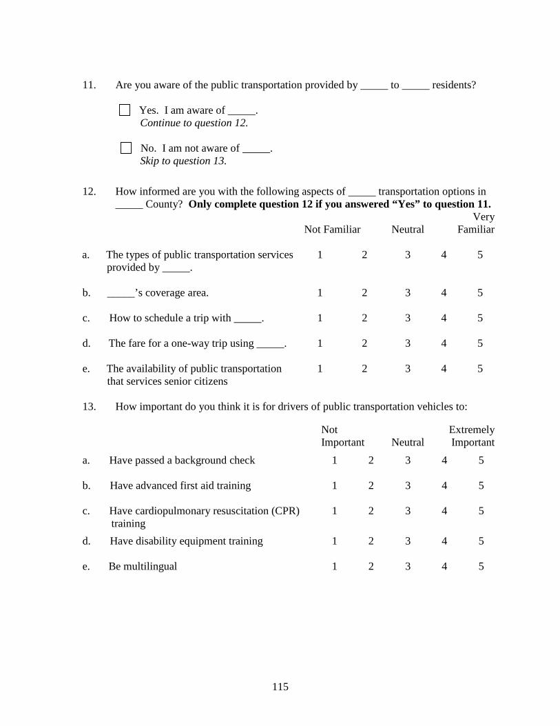
115
11. Are you aware of the public transportation provided by _____ to _____ residents?
Yes. I am aware of _____.
Continue to question 12.
No. I am not aware of _____. Skip to question 13.
12. How informed are you with the following aspects of _____ transportation options in _____ County? Only complete question 12 if you answered “Yes” to question 11.
Not Familiar
Neutral
Very Familiar
a. The types of public transportation services
provided by _____.
1
2
3
4
5
b. _____’s coverage area.
1 2 3 4 5
c. How to schedule a trip with _____.
1 2 3 4 5
d. The fare for a one-way trip using _____.
1 2 3 4 5
e. The availability of public transportation that services senior citizens
1 2 3 4 5
13. How important do you think it is for drivers of public transportation vehicles to:
Not Important
Neutral
Extremely Important
a. Have passed a background check
1 2 3 4 5
b. Have advanced first aid training
1 2 3 4 5
c. Have cardiopulmonary resuscitation (CPR) training
1 2 3 4 5
d. Have disability equipment training 1 2 3 4 5 e. Be multilingual
1
2
3
4
5

116
14. Based on your personal experiences, to what extent have age-related disabilities affected the driving ability of the following people? On the scale, 1 indicates individuals have little to no difficulty driving, whereas 5 indicates individuals have limited driving ability, to the point that they require assistance.
Little to no difficulty driving
Some
difficulty
Limited driving ability
a. Elderly family members
1 2 3 4 5
b. Elderly friends
1 2 3 4 5
If you are over the age of 75, please skip questions 15-17.
15. What do you feel is the percent chance (0-100%) that you will live to be 75 or older?
________________%
16. What do you feel is the percent chance (0-100%) that you will live, or continue
living, in a rural town or in the country (outside of town limits) when you are over the age of 75? _____________%
17. What do you feel is the percent chance (0-100%) that when you are over the age of
75, you will use alternative forms of transportation, such as rides from family and friends or public/private transportation options (i.e., buses or taxis)? ________________%
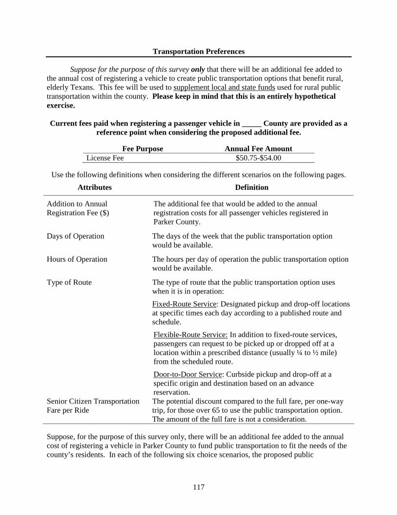
117
Transportation Preferences
Suppose for the purpose of this survey only that there will be an additional fee added to the annual cost of registering a vehicle to create public transportation options that benefit rural, elderly Texans. This fee will be used to supplement local and state funds used for rural public transportation within the county. Please keep in mind that this is an entirely hypothetical exercise.
Current fees paid when registering a passenger vehicle in _____ County are provided as a
reference point when considering the proposed additional fee.
Fee Purpose Annual Fee Amount License Fee $50.75-$54.00
Use the following definitions when considering the different scenarios on the following pages.
Attributes Definition
Addition to Annual Registration Fee ($)
The additional fee that would be added to the annual registration costs for all passenger vehicles registered in Parker County.
Days of Operation
The days of the week that the public transportation option would be available.
Hours of Operation
The hours per day of operation the public transportation option would be available.
Type of Route
The type of route that the public transportation option uses when it is in operation:
Fixed-Route Service: Designated pickup and drop-off locations at specific times each day according to a published route and schedule.
Flexible-Route Service: In addition to fixed-route services, passengers can request to be picked up or dropped off at a location within a prescribed distance (usually ¼ to ½ mile) from the scheduled route.
Door-to-Door Service: Curbside pickup and drop-off at a specific origin and destination based on an advance reservation.
Senior Citizen Transportation Fare per Ride
The potential discount compared to the full fare, per one-way trip, for those over 65 to use the public transportation option. The amount of the full fare is not a consideration.
Suppose, for the purpose of this survey only, there will be an additional fee added to the annual cost of registering a vehicle in Parker County to fund public transportation to fit the needs of the county’s residents. In each of the following six choice scenarios, the proposed public
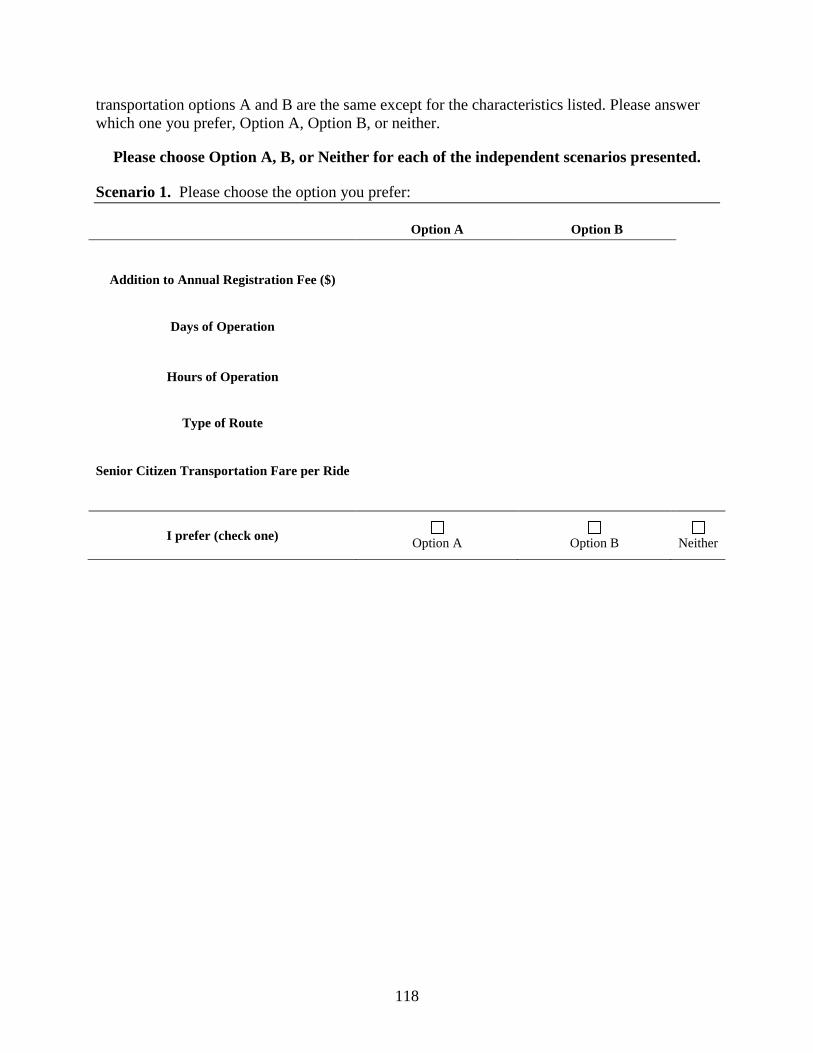
118
transportation options A and B are the same except for the characteristics listed. Please answer which one you prefer, Option A, Option B, or neither.
Please choose Option A, B, or Neither for each of the independent scenarios presented. Scenario 1. Please choose the option you prefer:
Option A Option B
Addition to Annual Registration Fee ($)
Days of Operation
Hours of Operation
Type of Route
Senior Citizen Transportation Fare per Ride
I prefer (check one) Option A
Option B
Neither
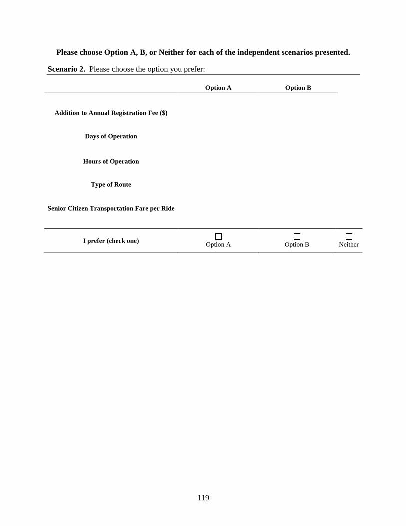
119
Please choose Option A, B, or Neither for each of the independent scenarios presented. Scenario 2. Please choose the option you prefer:
Option A Option B
Addition to Annual Registration Fee ($)
Days of Operation
Hours of Operation
Type of Route
Senior Citizen Transportation Fare per Ride
I prefer (check one) Option A
Option B
Neither
120
Please choose Option A, B, or Neither for each of the independent scenarios presented. Scenario 3. Please choose the option you prefer:
Option A Option B
Addition to Annual Registration Fee ($)
Days of Operation
Hours of Operation
Type of Route
Senior Citizen Transportation Fare per Ride
I prefer (check one) Option A
Option B
Neither
121
Please choose Option A, B, or Neither for each of the independent scenarios presented. Scenario 4. Please choose the option you prefer:
Option A Option B
Addition to Annual Registration Fee ($)
Days of Operation
Hours of Operation
Type of Route
Senior Citizen Transportation Fare per Ride
I prefer (check one) Option A
Option B
Neither

122
Please choose Option A, B, or Neither for each of the independent scenarios presented. Scenario 5. Please choose the option you prefer:
Option A Option B
Addition to Annual Registration Fee ($)
Days of Operation
Hours of Operation
Type of Route
Senior Citizen Transportation Fare per Ride
I prefer (check one) Option A
Option B
Neither
123
Please choose Option A, B, or Neither for each of the independent scenarios presented. Scenario 6. Please choose the option you prefer:
Option A Option B
Addition to Annual Registration Fee ($)
Days of Operation
Hours of Operation
Type of Route
Senior Citizen Transportation Fare per Ride
I prefer (check one) Option A
Option B
Neither
Please provide us with any comment(s) you have pertaining to this survey or the issue of providing transportation for the rural elderly.
Thank you for participating in this survey. Please return your completed questionnaire in the provided pre-paid
return envelope.


125
APPENDIX B. STUDENT SURVEY
Natural Resource & Environmental Economics Working Group Department of Agricultural Economics
Texas A&M University College Station, TX 77843-2124
Dear Fellow Aggie,
You are receiving this survey to assist me in my Master of Science thesis research concerning transportation options for rural elderly Texans. It is important to understand how all ages of the public view the needs of the elderly.
Texas has the fourth largest elderly population in the country. In 2009, more senior citizens lived
in rural areas than any other age group in Texas. This population is expected to continue to grow as baby boomers age and life expectancies increase. One central issue to the quality of life for rural senior citizens is their need for transportation options, specifically public transportation in their area.
Although it is popular in Texas for an individual to drive well into retirement, studies have shown that this is not always feasible or safe. Additionally, because of fixed, limited incomes, the elderly are not always able to afford a vehicle. If rural elderly individuals become unable to drive, there are few transportation options that provide the freedom and flexibility to make everyday trips such as running errands, social, and recreational outings, possibly leading to isolation and a decreased quality of life. The objective of this study is to determine the value that the general public places on attributes of public transportation which support the quality of life for current and future rural elderly individuals. Your contribution is vital in providing policymakers and transportation authorities with accurate information. Thank you for your help. Sincerely, Alicia A. Israel Class of 2010
126
Valuation and Opinions Concerning Transportation for the Rural Texas Elderly
Funded by the University Transportation Center for Mobility Texas Transportation Institute
Texas A&M University System College Station, TX
Participation in this survey is voluntary. You may decide not to participate or to withdraw at any time without your current or future relations with Texas A&M University being affected. This study is anonymous and no identifiable
information will be collected with your questionnaire.
If you have questions regarding this study, you may contact Alicia A. Israel at [email protected].
This research study has been reviewed by the Human Subjects’ Protection Program and/or the Institutional Review Board at Texas A&M University. For research-related problems or questions regarding your rights as a research
participant, you can contact these offices at (979)458-4067 or [email protected].
127
Valuation and Opinions Concerning Transportation for the Rural Texas Elderly
1. What is your classification at Texas A&M University?
a. Freshman
b. Sophomore
c. Junior
d. Senior
e. Other (please specify) _____________
2. What is your major? ____________________________________________________
3. What is your gender?
a. Male
b. Female
4. What is your age? _____________ years
5. What is your race?
a. Caucasian/White
b. Black, African American
c. American Indian or Alaskan Native
d. Hispanic
e. Asian, Pacific Islander
f. Multiracial
g. Other (please specify) _____________
6. What is your marital status?
a. Single
b. Married
c. Other (please specify) _____________

128
7. What percentage of funding for your total annual living and college expenses come from the following sources: The total of all percentages should equal 100%.
Parents/Guardians __________%
Self-funded (through working, savings, etc.) __________%
Scholarships and Grants __________%
Military __________%
Loans __________%
Other __________%
Total 100%
8. What city/town do you consider to be your home town?
Please provide City/County/State/Zip code
__________________________________________________________
9. How would you describe the area where your house in your home town is located?
a. Inside city or town limits
b. Outside city limits on a lot that is less than 5 acres
c. Outside city limits on a lot that is 5 acres or greater
d. On a working farm, or ranch
e. Other (please specify) _____________
10. Did you vote in the last national, state, or local elections? Please check all that apply.
National State Local None
11. Are there options to use public transportation in your home town?
As far as I know, there are no public transportation options in my home town. Skip to question 13.
Yes, there are public transportation options in my home town.
Continue to question 12.
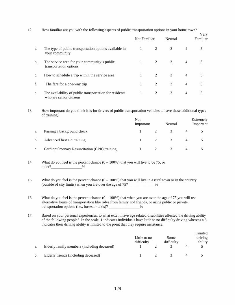
129
12. How familiar are you with the following aspects of public transportation options in your home town?
Not Familiar
Neutral
Very Familiar
a. The type of public transportation options available in
your community
1
2
3
4
5
b. The service area for your community’s public transportation options
1 2 3 4 5
c. How to schedule a trip within the service area
1 2 3 4 5
f. The fare for a one-way trip
1 2 3 4 5
e. The availability of public transportation for residents who are senior citizens
1 2 3 4 5
13. How important do you think it is for drivers of public transportation vehicles to have these additional types
of training?
Not Important
Neutral
Extremely Important
a. Passing a background check
1 2 3 4 5
b. Advanced first aid training
1 2 3 4 5
c. Cardiopulmonary Resuscitation (CPR) training 1 2 3 4 5 14. What do you feel is the percent chance (0 – 100%) that you will live to be 75, or
older?________________% 15. What do you feel is the percent chance (0 – 100%) that you will live in a rural town or in the country
(outside of city limits) when you are over the age of 75? _____________%
16. What do you feel is the percent chance (0 – 100%) that when you are over the age of 75 you will use alternative forms of transportation like rides from family and friends, or using public or private transportation options (i.e., buses or taxis)? ________________%
17. Based on your personal experiences, to what extent have age related disabilities affected the driving ability of the following people? In the scale, 1 indicates individuals have little to no difficulty driving whereas a 5 indicates their driving ability is limited to the point that they require assistance.
Little to no difficulty
Some
difficulty
Limited driving ability
a. Elderly family members (including deceased)
1 2 3 4 5
b. Elderly friends (including deceased)
1 2 3 4 5
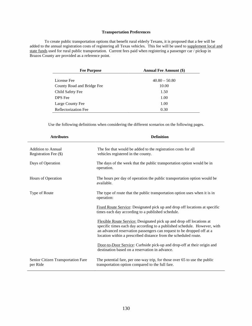
130
Transportation Preferences
To create public transportation options that benefit rural elderly Texans, it is proposed that a fee will be added to the annual registration costs of registering all Texas vehicles. This fee will be used to supplement local and state funds used for rural public transportation. Current fees paid when registering a passenger car / pickup in Brazos County are provided as a reference point.
Fee Purpose Annual Fee Amount ($) License Fee
40.80 – 50.80
County Road and Bridge Fee 10.00 Child Safety Fee 1.50 DPS Fee 1.00 Large County Fee 1.00 Reflectorization Fee 0.30
Use the following definitions when considering the different scenarios on the following pages.
Attributes Definition
Addition to Annual Registration Fee ($)
The fee that would be added to the registration costs for all vehicles registered in the county.
Days of Operation
The days of the week that the public transportation option would be in operation.
Hours of Operation
The hours per day of operation the public transportation option would be available.
Type of Route
The type of route that the public transportation option uses when it is in operation: Fixed Route Service: Designated pick up and drop off locations at specific times each day according to a published schedule. Flexible Route Service: Designated pick up and drop off locations at specific times each day according to a published schedule. However, with an advanced reservation passengers can request to be dropped off at a location within a prescribed distance from the scheduled route. Door-to-Door Service: Curbside pick-up and drop-off at their origin and destination based on a reservation in advance.
Senior Citizen Transportation Fare per Ride
The potential fare, per one-way trip, for those over 65 to use the public transportation option compared to the full fare.
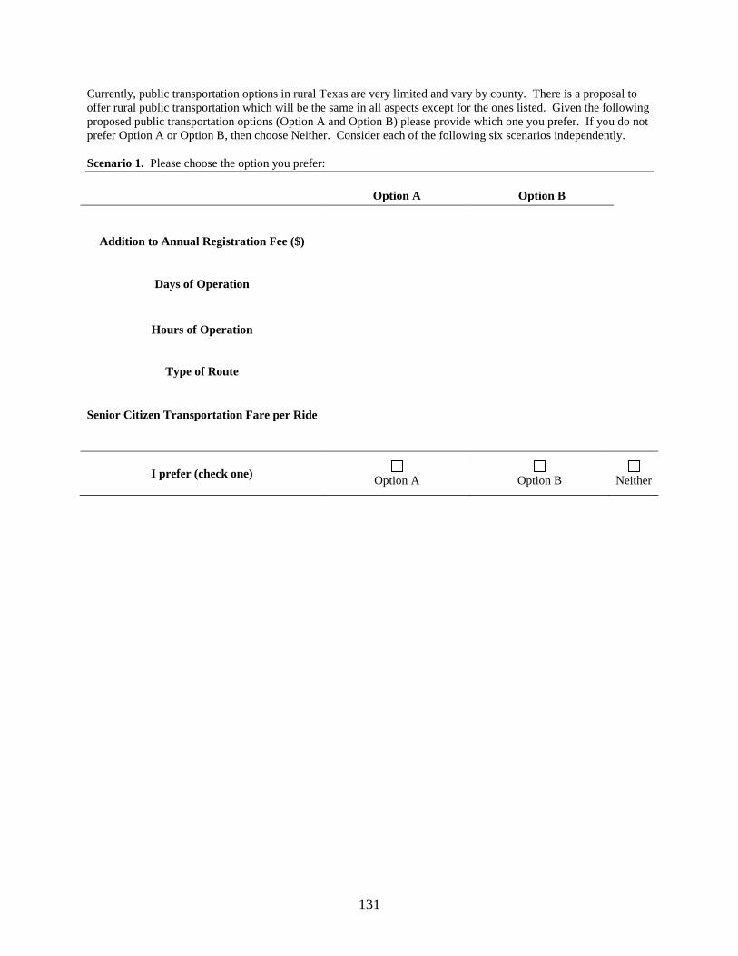
131
Currently, public transportation options in rural Texas are very limited and vary by county. There is a proposal to offer rural public transportation which will be the same in all aspects except for the ones listed. Given the following proposed public transportation options (Option A and Option B) please provide which one you prefer. If you do not prefer Option A or Option B, then choose Neither. Consider each of the following six scenarios independently. Scenario 1. Please choose the option you prefer:
Option A Option B
Addition to Annual Registration Fee ($)
Days of Operation
Hours of Operation
Type of Route
Senior Citizen Transportation Fare per Ride
I prefer (check one) Option A
Option B
Neither
132
Scenario 2. Please choose the option you prefer:
Option A Option B
Addition to Annual Registration Fee ($)
Days of Operation
Hours of Operation
Type of Route
Senior Citizen Transportation Fare per Ride
I prefer (check one) Option A
Option B
Neither

133
Scenario 3. Please choose the option you prefer:
Option A Option B
Addition to Annual Registration Fee ($)
Days of Operation
Hours of Operation
Type of Route
Senior Citizen Transportation Fare per Ride
I prefer (check one) Option A
Option B
Neither

134
Scenario 4. Please choose the option you prefer:
Option A Option B
Addition to Annual Registration Fee ($)
Days of Operation
Hours of Operation
Type of Route
Senior Citizen Transportation Fare per Ride
I prefer (check one) Option A
Option B
Neither

135
Scenario 5. Please choose the option you prefer:
Option A Option B
Addition to Annual Registration Fee ($)
Days of Operation
Hours of Operation
Type of Route
Senior Citizen Transportation Fare per Ride
I prefer (check one) Option A
Option B
Neither
136
Scenario 6. Please choose the option you prefer:
Option A Option B
Addition to Annual Registration Fee ($)
Days of Operation
Hours of Operation
Type of Route
Senior Citizen Transportation Fare per Ride
I prefer (check one) Option A
Option B
Neither
Thank you for your participating in this survey. Please return your completed questionnaire before leaving the classroom.

University Transportation Center for Mobility™
Texas Transportation Institute
The Texas A&M University System
College Station, TX 77843-3135
Tel: 979.845.2538 Fax: 979.845.9761
utcm.tamu.edu
TexasTransportationInstitute