Reinforced Multicategory Support Vector Machinesjgxchen/Fall2011/Reinforced Multicategory SVM.pdfSupplementary materials for this article are available online. PleaseclicktheJCGSlinkat

Supplementary materials for this article are available online.Please click the JCGS link at http://pubs.amstat.org.

Reinforced Multicategory Support VectorMachines

Yufeng LIU and Ming YUAN

Support vector machines are one of the most popular machine learning methods forclassification. Despite its great success, the SVM was originally designed for binaryclassification. Extensions to the multicategory case are important for general classifica-tion problems. In this article, we propose a new class of multicategory hinge loss func-tions, namely reinforced hinge loss functions. Both theoretical and numerical propertiesof the reinforced multicategory SVMs (MSVMs) are explored. The results indicate thatthe proposed reinforced MSVMs (RMSVMs) give competitive and stable performancewhen compared with existing approaches. R implementation of the proposed methodsis also available online as supplemental materials.

Key Words: Fisher consistency; Multicategory classification; Regularization; SVM.

1. INTRODUCTION

Classification is a very important statistical task for information extraction from data.Among numerous classification techniques, the Support Vector Machine (SVM) is one ofthe most well-known large-margin classifiers and has achieved great success in many ap-plications (Boser, Guyon, and Vapnik 1992; Cortes and Vapnik 1995). The basic conceptbehind the binary SVM is to find a separating hyperplane with maximum separation be-tween the two classes. Because of its flexibility in estimating the decision boundary usingkernel learning as well as its ability in handling high-dimensional data, the SVM has be-come a very popular classifier and has been widely applied in many different fields. Moredetails about the SVM can be found, for example, in the works of Cristianini and Shawe-Taylor (2000), Hastie, Tibshirani, and Friedman (2001), Schölkopf and Smola (2002).

Recent theoretical developments provide us more insight on the success of the SVM.Lin (2004) showed Fisher consistency of binary SVMs in the sense that the theoreticalminimizer of the hinge loss yields the Bayes classification boundary. As a result, the SVM

Yufeng Liu is Associate Professor, Department of Statistics and Operations Research, University of North Car-olina at Chapel Hill, Chapel Hill, NC 27599 (E-mail: [email protected]). Ming Yuan is Associate Professor,School of Industrial and Systems Engineering, Georgia Institute of Technology, Atlanta, GA 30332-0205 (E-mail:[email protected]).

1

© 2011 American Statistical Association, Institute of Mathematical Statistics,and Interface Foundation of North America

Journal of Computational and Graphical Statistics, Accepted for publication, Pages 1–19DOI: 10.1198/jcgs.2010.09206

http://pubs.amstat.org

mailto:[email protected]

mailto:[email protected]

http://www.amstat.org

http://www.imstat.org

http://www.galaxy.gmu.edu/stats/IFNA7.html

http://www.amstat.org/publications/jcgs

http://dx.doi.org/10.1198/jcgs.2010.09206

2 Y. LIU AND M. YUAN

targets on the decision boundary directly without estimating the conditional class proba-bility. More theoretical characterization of general binary large margin losses can be foundin the articles by Zhang (2004b), Bartlett, Jordan, and McAuliffe (2006).

The standard SVM only solves binary problems. However, one often encounters multi-category problems in practice. To solve a multicategory problem using the SVM, typicallythere are two possible approaches. The first approach is to solve the multicategory prob-lem via a sequence of binary problems, for example, one-versus-rest and one-versus-one(Dietterich and Bakiri 1995; Allwein et al. 2000). The second approach is to generalize thebinary SVM to a simultaneous multicategory formulation which deals with all classes atonce (Vapnik 1998; Weston and Watkins 1999; Crammer and Singer 2001; Lee, Lin, andWahba 2004; Liu and Shen 2006). The first approach is conceptually simple to implementsince one can use the existing binary techniques directly to solve multicategory problems.Despite its simplicity, the one-versus-rest approach may be inconsistent when there is nodominating class (Liu 2007). On the contrary, Rifkin and Klautau (2004) showed that theone-versus-rest approach can work as accurately as other simultaneous classification meth-ods using a substantial collection of numerical comparisons.

In this article, we reformulate the one-versus-rest approach as an instance of the si-multaneous multicategory formulation and focus on various simultaneous extensions. Inparticular, we propose a convex combination of an existing consistent multicategory hingeloss and another direct generalized hinge loss. Since the two components of the combina-tion intend to enforce correct classification in a complementary fashion, we call this familyof loss functions the reinforced multicategory hinge loss. We show that the proposed fam-ily of loss functions gives rise to a continuum of loss functions that are Fisher consistent.Moreover, the proposed reinforced multicategory SVM (RMSVM) appears to deliver moreaccurate classification results than the uncombined ones.

The rest of this article is organized as follows. In Section 2.1, we introduce the newreinforced hinge loss functions. Section 2.2 studies Fisher consistency of the new class ofloss functions. A computational algorithm of the RMSVM is given in Section 3. In Sec-tion 4, we use both simulated examples and an application to lung cancer Microarray datato illustrate performance of the proposed RMSVMs with different choices of the combin-ing weight parameter. Some discussion and remarks are given in Section 5, followed byproofs of the theoretical results in the Appendix.

2. METHODOLOGY

2.1 REINFORCED MULTICATEGORY HINGE LOSSES

Suppose we are given a training dataset containing n training pairs {xi , yi}ni=1, iid real-izations from probability distribution P(x, y), where x is the d-dimensional input and y isthe corresponding class label. For simplicity, we consider x ∈ �d . Our method, however,may be easily extended to include discrete and categorical input variables. For simplicity,in the rest of the article, we shall focus only on the standard learning where all types ofmisclassification are treated equally. The discussion, however, can be extended straightfor-wardly to more general settings with unequal losses.

REINFORCED MULTICATEGORY SUPPORT VECTOR MACHINES 3

In the binary case, the goal is to search for a function f (x) so that sign(f (x)) can beused for prediction of class labels for new inputs. The standard binary SVM can be viewedas an example of the regularization framework (Wahba 1999) as follows:

minf

[λJ (f ) + 1

n

n∑i=1

V (yif (xi ))

],

where J (f ) is the roughness penalty of f , V is the hinge loss with V (u) = [1 − u]+ =1 − u if u ≤ 1 and 0 otherwise, and λ ≥ 0 is a tuning parameter. Denote P(x) = P(Y =1|X = x). Lin (2004) showed that the minimizer of E[V (Yf (X))|X = x] has the samesign as P(x) − 1/2 and consequently the hinge loss of SVM targets on the Bayes decisionboundary asymptotically. This property is known as Fisher consistency and it is a desirablecondition for a loss function in classification.

Extension of the SVM from the binary to multicategory case is nontrivial and the keyis the generalization of the binary hinge loss to the multicategory case. Consider a k-classclassification problem with k ≥ 2. Let f = (f1, f2, . . . , fk) be the decision function vector,where each component represents one class and maps from �d to �. For any new inputvector x, its label is estimated via a decision rule y = argmaxj=1,2,...,k fj (x). Clearly, theargmax rule is equivalent to the sign function used in the binary case if a sum-to-zeroconstraint

∑kj=1 fj = 0 is employed.

Similarly to the binary case, we consider solving the following problem in order tolearn f:

minf

[λ

k∑j=1

J (fj ) + 1

n

n∑i=1

V (f(xi ), yi)

], (2.1)

subject to∑k

j=1 fj (x) = 0. Here, a sum-to-zero constraint is used to remove redundancyand reduce the dimension of the problem. Note that a point (x, y) is misclassified by f ify �= argmaxj fj (x). Thus a sensible loss V should try to encourage fy to be the maximum.

In the literature, a number of extensions of the binary hinge loss to the multicate-gory case have been proposed. See, for example, the works by Vapnik (1998), Westonand Watkins (1999), Bredensteiner and Bennett (1999), Crammer and Singer (2001), Lee,Lin, and Wahba (2004), Liu and Shen (2006). In this article, we consider a new class ofmulticategory hinge loss functions as follows:

V (f(x), y) = γ [(k − 1) − fy(x)]+ + (1 − γ )∑j �=y

[1 + fj (x)]+ (2.2)

subject to∑k

j=1 fj (x) = 0, where γ ∈ [0,1]. We call the loss function (2.2) the reinforcedhinge loss function since there are two terms in the loss and both terms try to force fy tobe the maximum. We choose the constant to be k − 1 for the first part of the loss sinceif fj = −1 for ∀j �= y, fy = k − 1 using the sum-to-zero constraint. Thus k − 1 is anatural choice to use for the reinforced loss (2.2). The main motivation for this new lossfunction is based on the consideration of the argmax rule for multicategory problems. Inorder to get a correct classification result on a data point, we need to have the correspondingfy(x) to be the maximum among k different fj (x); j = 1, . . . , k. To that end, the first term


encourages fy to be big while the second term encourages other fj ’s to be small. As wewill discuss later, each separate term of the loss function has certain drawbacks in viewof consistency and empirical performance. The proposed combined loss, however, yieldsbetter classification performance.

With different choices of γ , (2.2) constitutes a large class of loss functions. When γ = 0,(2.2) reduces to

∑j �=y[1+fj (x)]+ subject to

∑kj=1 fj (x) = 0 and it is the same loss as the

one used by Lee, Lin, and Wahba (2004). When γ = 1/2, if we replace k − 1 in (2.2) by 1,it reduces to

∑kj=1[1−c

yj fj (x)]+, where c

yj = 1 if j = y and −1 otherwise. This is the loss

employed by the one-versus-rest approach (Weston 1999) except that the latter generallydoes not enforce the sum-to-zero constraint so that the minimization can be decoupled.Because of these connections, the new loss (2.2) can be viewed as a combination of theone-versus-rest approach and the simultaneous classification approach. Our emphasis isthe effect of different choices of γ on the resulting classifiers.

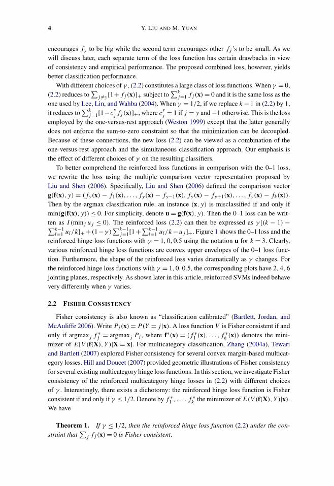
To better comprehend the reinforced loss functions in comparison with the 0–1 loss,we rewrite the loss using the multiple comparison vector representation proposed byLiu and Shen (2006). Specifically, Liu and Shen (2006) defined the comparison vectorg(f(x), y) = (fy(x) − f1(x), . . . , fy(x) − fy−1(x), fy(x) − fy+1(x), . . . , fy(x) − fk(x)).Then by the argmax classification rule, an instance (x, y) is misclassified if and only ifmin(g(f(x), y)) ≤ 0. For simplicity, denote u = g(f(x), y). Then the 0–1 loss can be writ-ten as I (minj uj ≤ 0). The reinforced loss (2.2) can then be expressed as γ [(k − 1) −∑k−1

l=1 ul/k]+ + (1−γ )∑k−1

j=1[1+∑k−1l=1 ul/k −uj ]+. Figure 1 shows the 0–1 loss and the

reinforced hinge loss functions with γ = 1,0,0.5 using the notation u for k = 3. Clearly,various reinforced hinge loss functions are convex upper envelopes of the 0–1 loss func-tion. Furthermore, the shape of the reinforced loss varies dramatically as γ changes. Forthe reinforced hinge loss functions with γ = 1,0,0.5, the corresponding plots have 2, 4, 6jointing planes, respectively. As shown later in this article, reinforced SVMs indeed behavevery differently when γ varies.

2.2 FISHER CONSISTENCY

Fisher consistency is also known as “classification calibrated” (Bartlett, Jordan, andMcAuliffe 2006). Write Pj (x) = P(Y = j |x). A loss function V is Fisher consistent if andonly if argmaxj f ∗

j = argmaxj Pj , where f∗(x) = (f ∗1 (x), . . . , f ∗

k (x)) denotes the mini-mizer of E[V (f(X), Y )|X = x]. For multicategory classification, Zhang (2004a), Tewariand Bartlett (2007) explored Fisher consistency for several convex margin-based multicat-egory losses. Hill and Doucet (2007) provided geometric illustrations of Fisher consistencyfor several existing multicategory hinge loss functions. In this section, we investigate Fisherconsistency of the reinforced multicategory hinge losses in (2.2) with different choicesof γ . Interestingly, there exists a dichotomy: the reinforced hinge loss function is Fisherconsistent if and only if γ ≤ 1/2. Denote by f ∗

1 , . . . , f ∗k the minimizer of E(V (f(X), Y )|x).

We have

Theorem 1. If γ ≤ 1/2, then the reinforced hinge loss function (2.2) under the con-straint that

∑j fj (x) = 0 is Fisher consistent.


Figure 1. Plots of various loss functions using u as the argument for k = 3: the 0–1 loss on the top-left panel,the reinforced hinge loss functions with γ = 1,0,0.5 on the top-right, bottom-left, bottom-right panels.

Theorem 1 establishes Fisher consistency of the reinforced hinge loss with γ ≤ 1/2.

Our next theorem explores the case of γ > 1/2.

Theorem 2. If k > 2, then for any γ > 1/2, there exists a set of P1(x) > P2(x) ≥ · · · ≥Pk(x) such that f ∗

1 (x) = f ∗2 (x) and therefore V (f(x), y) in (2.2) under the constraint that∑

j fj (x) = 0 is not always Fisher consistent.

The proofs are provided in the Appendix. From Theorems 1 and 2, we can conclude that

the proposed reinforced hinge loss is Fisher consistent if and only if 0 ≤ γ ≤ 1/2. This pro-

vides a large class of consistent multicategory hinge loss functions. When γ > 1/2, Fisher

consistency cannot be guaranteed when there is no dominating class, that is, maxj Pj (x) <

1/2. Modifications such as additional constraints as in the article by Liu (2007) may be ap-

plied to make the loss consistent. However, such modifications will result in loss functions

that are no longer hinge losses and are thus not pursued here.

Interestingly, as indicated by the numerical examples in Section 4, RMSVMs with the

values of γ in the middle range of [0,1] such as γ = 0.5 work better than those of γ = 0

or 1. This reflects the advantages of proposed combined loss functions which encourage fy

to be maximum both explicitly and implicitly through the two components in (2.2).


3. COMPUTATIONAL ALGORITHM

We now derive a computational algorithm for the RMSVM within the kernel learningframework. Using the representer theorem (Kimeldorf and Wahba 1971; Wahba 1999),fj (x) can be represented as bj + ∑n

i′=1 K(x,xi′)vi′j , where K(·, ·) is the kernel function,and bi, vi′j ; i′ = 1, . . . , n are coefficients for fj . Then we have

fj (xi ) = bj +n∑

i′=1

K(xi ,xi′)vi′j = bj + KTi v·j , (3.1)

where Ki = (K(xi ,x1),K(xi ,x2), . . . ,K(xi ,xn))T and v·j = (v1j , . . . , vnj )

T . Moreover,J (fj ) = 1

2 vT·j Kv·j . Thus the RMSVM can be reduced to

min�

λ

2

k∑j=1

vT·j Kv·j + 1

n

n∑i=1

(γ[(k − 1) − byi

− KTi v·yi

]+

+ (1 − γ )∑j �=yi

[1 + bj + KTi v·j ]+

), (3.2)

s.t. ek∑

j=1

bj + Kk∑

j=1

v·j = 0,

where � denotes {v·j , bj }kj=1, K denotes the kernel matrix with the (i, i′) element beingK(xi ,xi′), and e = (1,1, . . . ,1)T is a vector of length n.

To solve (3.2), we introduce nonnegative slack variables ξij ; i = 1, . . . , n, j = 1, . . . , k,

and then the primal problem of our RMSVM can be written as

min�,ξ

nλ

2

k∑j=1

vT·j Kv·j +n∑

i=1

(γ ξiyi

+ (1 − γ )∑j �=yi

ξij

),

s.t. ξij ≥ 0; i = 1, . . . , n, j = 1, . . . , k,

ξiyi+ (

byi+ KT

i v·yi− (k − 1)

) ≥ 0; i = 1, . . . , n,

ξij − (bj + KT

i v·j + 1) ≥ 0; i = 1, . . . , n, j �= yi,(

k∑j=1

bj

)e + K

(k∑

j=1

v·j

)= 0.

The corresponding Lagrangian function is

LD = nλ

2

k∑j=1

vT·j Kv·j +n∑

i=1

(γ ξiyi

+ (1 − γ )∑j �=yi

ξij

)

−n∑

i=1

k∑j=1

τij ξij + δT

(K

(k∑

j=1

v·j

)+

(k∑

j=1

bj

)e

)


−n∑

i=1

αiyi

(ξiyi

+ byi+ KT

i v·yi− (k − 1)

) −n∑

i=1

∑j �=yi

αij (ξij − bj − KTi v·j − 1)

= nλ

2

k∑j=1

vT·j Kv·j +n∑

i=1

k∑j=1

(Aij − τij − αij )ξij +n∑

i=1

(k − 1)αiyi+

n∑i=1

∑j �=yi

αij

+k∑

j=1

bj

(−(α·j · (e − L·j ))T e + (α·j · L·j )T e + δT e)

+k∑

j=1

⟨K(α·j · L·j ) − K(α·j · (e − L·j )) + Kδ,v·j

⟩,

where αij ≥ 0 and τij ≥ 0, δ = (δ1, δ2, . . . , δn)T are Lagrangian multipliers, L·j is a vec-

tor of length n with its ith element being 0 if yi = j and 1 otherwise, α·j · L·j denotescomponentwise product between α·j and L·j , and Aij = [γ I (yi = j)+ (1−γ )I (yi �= j)].Setting ∂LD

∂ξij= 0, ∂LD

∂bj= 0, and ∂LD

∂v·j = 0, we have

∂LD

∂ξij

= Aij − τij − αij = 0, (3.3)

∂LD

∂bj

= −(α·j · (e − L·j ))T e + (α·j · L·j )T e + δT e = 0, (3.4)

∂LD

∂v·j= nλKv·j + K(α·j · L·j ) + Kδ − K(α·j · (e − L·j )) = 0. (3.5)

Due to the positive definitive kernel K(·, ·), (3.5) implies that v·j = 1nλ

(α·j · (e − L·j )−α·j ·L·j −δ). Let α = 1

k

∑kj=1(α·j ·L·j ) and ¯α = 1

k

∑kj=1(α·j · (e−L·j )). Then from (3.4)

and (3.5), we have δ = ¯α − α and

v·j = 1

nλ[(α·j · (e − L·j ) − α·j · L·j ) − ( ¯α − α)]. (3.6)

After plugging (3.3)–(3.6) into LD , we can derive the corresponding dual problem as fol-lows:

minα

1

2

k∑j=1

⟨[(α·j · (e − L·j ) − α·j · L·j ) − ( ¯α − α)

],

K[(α·j · (e − L·j ) − α·j · L·j ) − ( ¯α − α)

]⟩−nλ

n∑i=1

(k − 1)αiyi− nλ

n∑i=1

∑j �=yi

αij , (3.7)

s.t. 0 ≤ αij ≤ Aij ; i = 1, . . . , n, j = 1, . . . , k,

[(α·j · (e − L·j ) − α·j · L·j ) − ( ¯α − α)]T e = 0; j = 1, . . . , k.


To further simplify (3.7), define β = (αT·1, . . . ,αT·k)T , ej as a vector of length k withits j th element being 1 and the remaining ones being 0, Uj = eT

j ⊗ In, and Vj as a di-agonal matrix with L·j as the diagonal elements, where ⊗ denotes the Kronecker productand In denotes the n × n identity matrix. Then α·j · L·j = VjUjβ and α·j · (e − L·j ) =(In − Vj )Ujβ . Furthermore, (3.7) can be simplified as the following quadratic program-ming (QP) problem:

minβ

1

2βT

k∑j=1

HTj KHjβ + gT β,

s.t. 0 ≤ αij ≤ Aij ; i = 1, . . . , n, j = 1, . . . , k, (3.8)

eT Hjβ = 0; j = 1, . . . , k,

where Hj = (In − Vj )Uj − VjUj − 1k

∑km=1(In − Vm)Um + 1

k

∑km=1 VmUm and g is a

vector of length nk with its (j − 1)n + ith elements being −nλ(k − 1) if j = yi and −nλ

otherwise.Once {vj ; j = 1, . . . , k} are obtained, we can solve b either by the KKT conditions or

linear programming (LP). More explicitly, with {vj ; j = 1, . . . , k} given, we can obtain bby solving

minb,η

k∑j=1

(γ ηiyi

+ (1 − γ )∑j �=yi

ηij

),

subject tok∑

j=1

bj = 0,

ηij ≥ 0; i = 1, . . . , n, j = 1, . . . , k, (3.9)

ηiyi+ (

byi+ KT

i v·yi− (k − 1)

) ≥ 0; i = 1, . . . , n,

ηij − (bj + KTi v·j + 1) ≥ 0; i = 1, . . . , n, j �= yi.

Our algorithm for the RMSVM with a given λ can be summarized as follows:Step 1: Solve the QP problem (3.8) to obtain solution β .Step 2: With β given, solve (3.6) to get the solution for v·j ; j = 1, . . . , k.Step 3: With {vj ; j = 1, . . . , k} given, b can be derived by solving the LP problem (3.9).

4. NUMERICAL EXAMPLES

4.1 SIMULATION

In this section, we use two simulated examples to examine the behavior of the RMSVMsand how their performance varies with γ . Since γ ∈ [0,1], we examine 11 choices withγ = 0,0.1, . . . ,1. As shown in Theorems 1 and 2, the RMSVMs have Fisher consistencyfor γ ∈ [0,0.5] and are not always Fisher consistent for γ > 0.5. Thus, these values of γ

should provide a broad range of behaviors of the corresponding RMSVMs. The case ofγ = 0 corresponds to the version by Lee, Lin, and Wahba (2004).


4.1.1 Example With a Piecewise Linear Bayes Decision Boundary

In this three-class example, P(Y = 1) = P(Y = 2) = P(Y = 3) = 1/3, P(X|Y = 1) ∼N(μ = (0,2)T ,1.52I2), P(X|Y = 2) ∼ N(μ = (−√

3,−1)T ,1.52I2), and P(X|Y = 3) ∼N(μ = (

√3,−1)T ,1.52I2). Due to the design of this example, linear learning can be suf-

ficient and the corresponding Bayes boundary is piecewise linear as displayed in the leftpanel of Figure 3 below.

We simulate n observations for training, n observations for tuning, and a large set fortesting. We use the training set to build RMSVM classifiers and then use the separatetuning set to choose the tuning parameter λ among the set {2−16,2−15, . . . ,215}. After thetuning parameter gets selected, we use the test set to evaluate the corresponding test errorof the tuned RSVMs. To examine the effect of different choices of the function class, weuse both linear kernel, K(u,v) = 〈u,v〉, and the polynomial kernel of order 2, K(u,v) =(1 + 〈u,v〉)2.

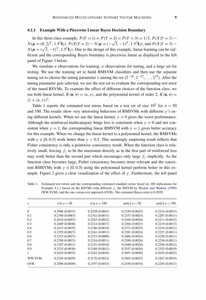
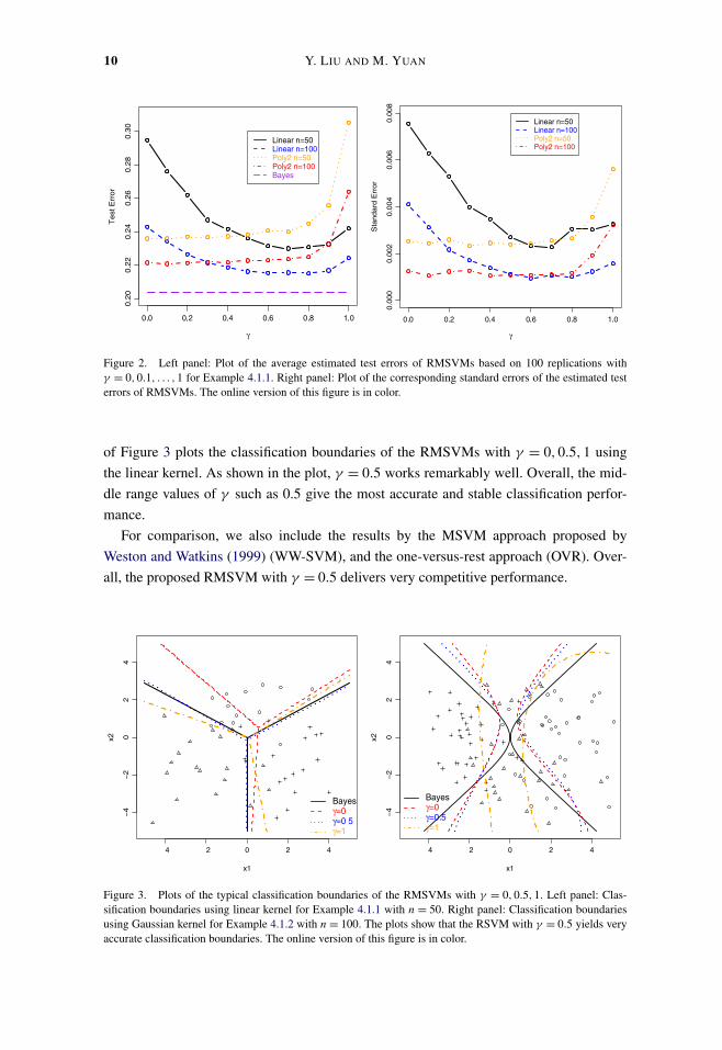
Table 1 reports the estimated test errors based on a test set of size 105 for n = 50and 100. The results show very interesting behaviors of RMSVMs with different γ ’s us-ing different kernels. When we use the linear kernel, γ = 0 gives the worst performance.Although the reinforced multicategory hinge loss is consistent when γ = 0 and not con-sistent when γ = 1, the corresponding linear RMSVM with γ = 1 gives better accuracyfor this example. When we change the linear kernel to a polynomial kernel, the RMSVMswith γ ∈ [0,0.5] work better than γ > 0.5. This seemingly surprising result reflects thatFisher consistency is only a pointwise consistency result. When the function class is rela-tively small, forcing fy to be the maximum directly as in the first part of reinforced lossmay work better than the second part which encourages only large fy implicitly. As thefunction class becomes large, Fisher consistency becomes more relevant and the consis-tent RMSVMs with γ ∈ [0,0.5] using the polynomial kernel perform better in this ex-ample. Figure 2 gives a clear visualization of the effect of γ . Furthermore, the left panel

Table 1. Estimated test errors and the corresponding estimated standard errors based on 100 replications forExample 4.1.1 based on the RSVMs with different γ , the MSVM by Weston and Watkins (1999)(WW-SVM), and the one-versus-rest approach (OVR). The estimated Bayes error is 0.2039.

γ Lin n = 50 Lin n = 100 poly2 n = 50 poly2 n = 100

0 0.2948 (0.0075) 0.2428 (0.0041) 0.2359 (0.0025) 0.2214 (0.0013)0.1 0.2760 (0.0063) 0.2342 (0.0031) 0.2357 (0.0024) 0.2207 (0.0011)0.2 0.2618 (0.0053) 0.2263 (0.0022) 0.2368 (0.0026) 0.2211 (0.0012)0.3 0.2469 (0.0040) 0.2214 (0.0017) 0.2366 (0.0023) 0.2219 (0.0013)0.4 0.2415 (0.0035) 0.2186 (0.0014) 0.2371 (0.0025) 0.2216 (0.0011)0.5 0.2359 (0.0027) 0.2161 (0.0011) 0.2381 (0.0024) 0.2227 (0.0011)0.6 0.2315 (0.0023) 0.2153 (0.0009) 0.2406 (0.0024) 0.2230 (0.0011)0.7 0.2298 (0.0023) 0.2154 (0.0011) 0.2399 (0.0026) 0.2236 (0.0011)0.8 0.2307 (0.0031) 0.2151 (0.0010) 0.2448 (0.0026) 0.2249 (0.0012)0.9 0.2325 (0.0030) 0.2168 (0.0012) 0.2557 (0.0036) 0.2325 (0.0019)1 0.2419 (0.0033) 0.2242 (0.0016) 0.3051 (0.0056) 0.2639 (0.0032)

WW-SVM 0.2359 (0.0029) 0.2176 (0.0012) 0.2505 (0.0032) 0.2267 (0.0019)

OVR 0.2506 (0.0049) 0.2197 (0.0015) 0.2550 (0.0034) 0.2256 (0.0013)


Figure 2. Left panel: Plot of the average estimated test errors of RMSVMs based on 100 replications withγ = 0,0.1, . . . ,1 for Example 4.1.1. Right panel: Plot of the corresponding standard errors of the estimated testerrors of RMSVMs. The online version of this figure is in color.

of Figure 3 plots the classification boundaries of the RMSVMs with γ = 0,0.5,1 using

the linear kernel. As shown in the plot, γ = 0.5 works remarkably well. Overall, the mid-

dle range values of γ such as 0.5 give the most accurate and stable classification perfor-

mance.

For comparison, we also include the results by the MSVM approach proposed by

Weston and Watkins (1999) (WW-SVM), and the one-versus-rest approach (OVR). Over-

all, the proposed RMSVM with γ = 0.5 delivers very competitive performance.

Figure 3. Plots of the typical classification boundaries of the RMSVMs with γ = 0,0.5,1. Left panel: Clas-sification boundaries using linear kernel for Example 4.1.1 with n = 50. Right panel: Classification boundariesusing Gaussian kernel for Example 4.1.2 with n = 100. The plots show that the RSVM with γ = 0.5 yields veryaccurate classification boundaries. The online version of this figure is in color.


4.1.2 Example With a Nonlinear Bayes Decision Boundary

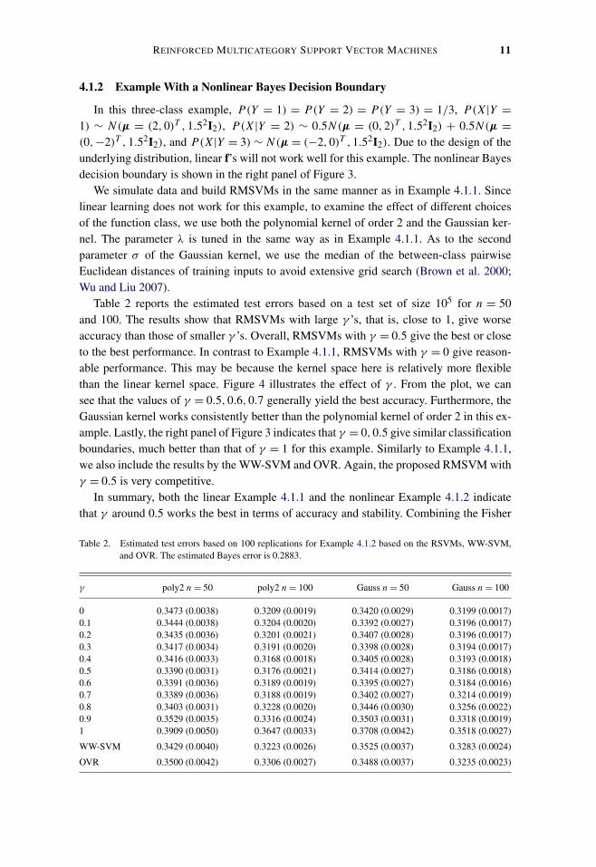
In this three-class example, P(Y = 1) = P(Y = 2) = P(Y = 3) = 1/3, P(X|Y =1) ∼ N(μ = (2,0)T ,1.52I2), P(X|Y = 2) ∼ 0.5N(μ = (0,2)T ,1.52I2) + 0.5N(μ =(0,−2)T ,1.52I2), and P(X|Y = 3) ∼ N(μ = (−2,0)T ,1.52I2). Due to the design of theunderlying distribution, linear f’s will not work well for this example. The nonlinear Bayesdecision boundary is shown in the right panel of Figure 3.

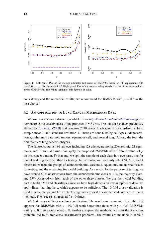
We simulate data and build RMSVMs in the same manner as in Example 4.1.1. Sincelinear learning does not work for this example, to examine the effect of different choicesof the function class, we use both the polynomial kernel of order 2 and the Gaussian ker-nel. The parameter λ is tuned in the same way as in Example 4.1.1. As to the secondparameter σ of the Gaussian kernel, we use the median of the between-class pairwiseEuclidean distances of training inputs to avoid extensive grid search (Brown et al. 2000;Wu and Liu 2007).

Table 2 reports the estimated test errors based on a test set of size 105 for n = 50and 100. The results show that RMSVMs with large γ ’s, that is, close to 1, give worseaccuracy than those of smaller γ ’s. Overall, RMSVMs with γ = 0.5 give the best or closeto the best performance. In contrast to Example 4.1.1, RMSVMs with γ = 0 give reason-able performance. This may be because the kernel space here is relatively more flexiblethan the linear kernel space. Figure 4 illustrates the effect of γ . From the plot, we cansee that the values of γ = 0.5,0.6,0.7 generally yield the best accuracy. Furthermore, theGaussian kernel works consistently better than the polynomial kernel of order 2 in this ex-ample. Lastly, the right panel of Figure 3 indicates that γ = 0,0.5 give similar classificationboundaries, much better than that of γ = 1 for this example. Similarly to Example 4.1.1,we also include the results by the WW-SVM and OVR. Again, the proposed RMSVM withγ = 0.5 is very competitive.

In summary, both the linear Example 4.1.1 and the nonlinear Example 4.1.2 indicatethat γ around 0.5 works the best in terms of accuracy and stability. Combining the Fisher

Table 2. Estimated test errors based on 100 replications for Example 4.1.2 based on the RSVMs, WW-SVM,and OVR. The estimated Bayes error is 0.2883.

γ poly2 n = 50 poly2 n = 100 Gauss n = 50 Gauss n = 100

0 0.3473 (0.0038) 0.3209 (0.0019) 0.3420 (0.0029) 0.3199 (0.0017)0.1 0.3444 (0.0038) 0.3204 (0.0020) 0.3392 (0.0027) 0.3196 (0.0017)0.2 0.3435 (0.0036) 0.3201 (0.0021) 0.3407 (0.0028) 0.3196 (0.0017)0.3 0.3417 (0.0034) 0.3191 (0.0020) 0.3398 (0.0028) 0.3194 (0.0017)0.4 0.3416 (0.0033) 0.3168 (0.0018) 0.3405 (0.0028) 0.3193 (0.0018)0.5 0.3390 (0.0031) 0.3176 (0.0021) 0.3414 (0.0027) 0.3186 (0.0018)0.6 0.3391 (0.0036) 0.3189 (0.0019) 0.3395 (0.0027) 0.3184 (0.0016)0.7 0.3389 (0.0036) 0.3188 (0.0019) 0.3402 (0.0027) 0.3214 (0.0019)0.8 0.3403 (0.0031) 0.3228 (0.0020) 0.3446 (0.0030) 0.3256 (0.0022)0.9 0.3529 (0.0035) 0.3316 (0.0024) 0.3503 (0.0031) 0.3318 (0.0019)1 0.3909 (0.0050) 0.3647 (0.0033) 0.3708 (0.0042) 0.3518 (0.0027)

WW-SVM 0.3429 (0.0040) 0.3223 (0.0026) 0.3525 (0.0037) 0.3283 (0.0024)

OVR 0.3500 (0.0042) 0.3306 (0.0027) 0.3488 (0.0037) 0.3235 (0.0023)


Figure 4. Left panel: Plot of the average estimated test errors of RMSVMs based on 100 replications withγ = 0,0.1, . . . ,1 for Example 4.1.2. Right panel: Plot of the corresponding standard errors of the estimated testerrors of RMSVMs. The online version of this figure is in color.

consistency and the numerical results, we recommend the RMSVM with γ = 0.5 as thebest choice.

4.2 AN APPLICATION TO LUNG CANCER MICROARRAY DATA

We use a real cancer dataset (available from http://www.broad.mit.edu/mpr/ lung/ ) todemonstrate the effectiveness of the proposed RMSVMs. The dataset has been previouslystudied by Liu et al. (2008) and contains 2530 genes. Each gene is standardized to havesample mean 0 and standard deviation 1. There are four histological types, adenocarci-noma, pulmonary carcinoid tumors, squamous cell, and normal lung. Among the four, thefirst three are lung cancer subtypes.

The dataset contains 186 subjects including 128 adenocarcinoma, 20 carcinoid, 21 squa-mous, and 17 normal tissues. We apply the proposed RMSVMs with different values of γ

on this cancer dataset. To that end, we split the sample of each class into two parts, one formodel building and the other for testing. In particular, we randomly select 64, 5, 5, and 4observations from the groups of adenocarcinoma, carcinoid, squamous, and normal tissuesfor testing, and the remaining for model building. As a result, for the purpose of testing, wehave around 50% observations from the adenocarcinoma class as it is the majority class,and 25% observations from each of the other three classes. We use the model buildingpart to build RMSVM classifiers. Since we have high-dimension low-sample-size data, weapply linear learning here, which appears to be sufficient. The 10-fold cross-validation isused to select the parameter λ. The testing data are used to evaluate and compare differentmethods. The process is repeated for 10 times.

We first carry out the four-class classification. The results are summarized in Table 3. Itappears that RMSVMs with γ ∈ [0,0.5] work better than those with γ > 0.5. RMSVMswith γ ≤ 0.5 give same results. To further compare the methods, we split the four-classproblem into four three-class classification problems. The results are included in Table 3

http://www.broad.mit.edu/mpr/lung/


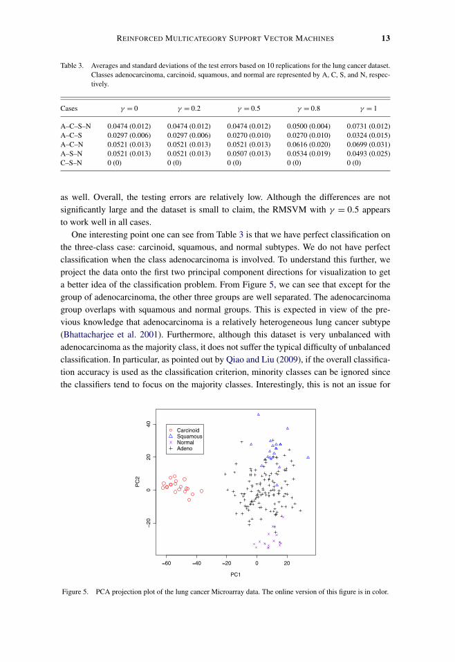
Table 3. Averages and standard deviations of the test errors based on 10 replications for the lung cancer dataset.Classes adenocarcinoma, carcinoid, squamous, and normal are represented by A, C, S, and N, respec-tively.

Cases γ = 0 γ = 0.2 γ = 0.5 γ = 0.8 γ = 1

A–C–S–N 0.0474 (0.012) 0.0474 (0.012) 0.0474 (0.012) 0.0500 (0.004) 0.0731 (0.012)A–C–S 0.0297 (0.006) 0.0297 (0.006) 0.0270 (0.010) 0.0270 (0.010) 0.0324 (0.015)A–C–N 0.0521 (0.013) 0.0521 (0.013) 0.0521 (0.013) 0.0616 (0.020) 0.0699 (0.031)A–S–N 0.0521 (0.013) 0.0521 (0.013) 0.0507 (0.013) 0.0534 (0.019) 0.0493 (0.025)C–S–N 0 (0) 0 (0) 0 (0) 0 (0) 0 (0)

as well. Overall, the testing errors are relatively low. Although the differences are notsignificantly large and the dataset is small to claim, the RMSVM with γ = 0.5 appearsto work well in all cases.

One interesting point one can see from Table 3 is that we have perfect classification onthe three-class case: carcinoid, squamous, and normal subtypes. We do not have perfectclassification when the class adenocarcinoma is involved. To understand this further, weproject the data onto the first two principal component directions for visualization to geta better idea of the classification problem. From Figure 5, we can see that except for thegroup of adenocarcinoma, the other three groups are well separated. The adenocarcinomagroup overlaps with squamous and normal groups. This is expected in view of the pre-vious knowledge that adenocarcinoma is a relatively heterogeneous lung cancer subtype(Bhattacharjee et al. 2001). Furthermore, although this dataset is very unbalanced withadenocarcinoma as the majority class, it does not suffer the typical difficulty of unbalancedclassification. In particular, as pointed out by Qiao and Liu (2009), if the overall classifica-tion accuracy is used as the classification criterion, minority classes can be ignored sincethe classifiers tend to focus on the majority classes. Interestingly, this is not an issue for

Figure 5. PCA projection plot of the lung cancer Microarray data. The online version of this figure is in color.


our example since the class of adenocarcinoma is the most difficult one to classify. Thereported classification errors are mostly due to adenocarcinoma.

5. DISCUSSION

In the literature, there exist a number of different multicategory SVMs. To our knowl-edge, most of them are not Fisher consistent. In this article, we propose the new family ofreinforced multicategory hinge loss functions. Our proposed RMSVMs include the MSVMby Lee, Lin, and Wahba (2004) as a special case, and also cover many new Fisher consis-tent multicategory hinge loss functions. Furthermore, the new family has some interestingconnections with the one-versus-rest approach.

Our theoretical investigation and numerical studies indicate that γ = 0.5 appears towork very well. Although we do not expect the RMSVM to always outperform other ex-isting MSVMs in real applications in view of the previous numerical study by Rifkin andKlautau (2004), Hill and Doucet (2007), we believe that the RMSVM provides a promisingand useful addition to the SVM toolkit.

In comparison with the one-versus-rest method, all-at-once methods such as theRMSVM can be more expensive to compute. For binary SVMs, Platt (1999) proposedSequential Minimal Optimization (SMO) to simplify the computation. Hill and Doucet(2007) extended the use of SMO for multicategory SVMs. One possible approach to re-duce the computational cost of the RMSVM is to adopt SMO. Another approach to improvecomputation is to develop efficient solution-path algorithms for the RMSVM (Hastie et al.2004; Wang and Shen 2006).

To implement the reinforced SVM in practice, one needs to choose the tuning parame-ter λ in (2.1). Similarly to many other regularization methods, the tuning parameter λ isimportant for the effectiveness of the proposed technique. Although one can use certaincross-validation procedures in practice when a separate tuning dataset is not available, thecomputational cost can be high. Therefore, an easy-to-compute data-dependent tuning cri-terion is desirable. Wahba, Lin, and Zhang (2000) developed the generalized approximatecross-validation (GACV) procedure for efficient tuning parameter selection of the SVM. Itwill be interesting to generalize the GACV procedures for our RMSVMs.

Another research direction of RMSVMs is the convergence properties. A number of ar-ticles on the convergence of large-margin classifiers have appeared in the literature. To lista few, Shen et al. (2003) provided learning theory for ψ -learning. Tarigan and van de Geer(2004), Wang and Shen (2007) derived rates of convergence for the L1 SVMs. Steinwartand Scovel (2006) studied the convergence rate of the SVM using Gaussian kernels. Re-cently, Shen and Wang (2007) studied rates of convergence of the generalization error of aclass of multicategory margin classifiers. It will be interesting to explore the effect of γ onthe RMSVM in terms of its asymptotic convergence behavior.

APPENDIX: PROOFS OF THE FISHER CONSISTENCY RESULTS

In this section, we give the proofs of Theorems 1 and 2. We begin by discussing Fisherconsistency of the two extremes: (I) γ = 1 and (II) γ = 0.


Lemma A.1. Assume that argminj Pj (x) is uniquely determined. The minimizer f∗ of

E[[(k −1)−fY (X)]+] subject to∑k

j fj (x) = 0 satisfies the following: f ∗j (x) = −(k −1)2

if j = argminj Pj (x) and k − 1 otherwise.

From Lemma A.1, we can see that the loss (I), [(k−1)−fy(x)]+ subject to∑k

j fj (x) =0, is not consistent since except the smallest element, all the remaining elements of itsminimizer are k − 1. Consequently, the argmax rule cannot be uniquely determined andthus the loss is not consistent.

Lemma A.2. Assume that argmaxj Pj (x) is uniquely determined. The minimizer f∗ of

E[∑j �=Y [1 + fj (X)]+] subject to∑k

j fj (x) = 0 satisfies the following: f ∗j (x) = k − 1 if

j = argmaxj Pj (x) and −1 otherwise.

Lemma A.2 implies that the loss (II),∑

j �=y[1 + fj (x)]+ subject to∑k

j fj (x) = 0, isa consistent loss since its minimizer yields the Bayes decision boundary. A similar resultwas also established by Lee, Lin, and Wahba (2004).

We now prove Lemmas A.1 and A.2 and then show several additional lemmas.

Proof of Lemma A.1: E[[(k − 1) − fY (X)]+] = E[∑kl=1[(k − 1) − fl(X)]+Pl(X)].

For any fixed X = x, our goal is to minimize∑k

l=1[(k − 1) − fl(x)]+Pl(x).We first show the minimizer f∗ satisfies f ∗

j ≤ (k − 1) for ∀j = 1, . . . , k. To this end,

suppose a solution f1 having f 1j > (k − 1). Then we can construct another solution f2 with

f 2j = (k − 1) and f 2

l = f 1l + A, where l �= j and A = (k − 1 − f 1

j )/(k − 1) > 0. Then∑l f

2l = 0 and f 2

l > f 1l ; ∀l �= j . Consequently,

∑kl=1[(k − 1) − f 2

l ]+Pl <∑k

l=1[(k −1) − f 1

l ]+Pl . This implies that f1 cannot be the minimizer. Therefore, the minimizer f∗satisfies f ∗

j ≤ (k − 1) for ∀j .Using the property of f∗, we only need to consider f with fj ≤ (k − 1) for ∀j . Thus,∑kl=1[(k − 1) − fl(x)]+Pl(x) = ∑k

l=1(k − 1 − fl(x))Pl(x) = k − 1 − ∑kl=1 fl(x)pl(x).

Then the problem reduces to

maxf

k∑l=1

Pl(x)fl(x),

subject tok∑

l=1

fl(x) = 0; fl(x) ≤ (k − 1) ∀l.

It is easy to see that the solution satisfies f ∗j (x) = −(k − 1)2 if j = argminj Pj (x) and

k − 1 otherwise. �

Proof of Lemma A.2: Note that E[∑j �=Y [1 + fj (X)]+] = E[E(∑

j �=Y [1 +fj (x)]+|X = x)]. Thus, it is sufficient to consider the minimizer for a given x andE(

∑j �=Y [1 + fj (x)]+|X = x) = ∑k

l=1∑

j �=l[1 + fj (x)]+Pl(x).Next, we show the minimizer f∗ satisfies f ∗

j ≥ −1 for ∀j = 1, . . . , k. To show this,

suppose a solution f1 having f 1j < −1. Then we can construct another solution f2 with


f 2j = −1 and f 2

l = f 1l − A, where A = (−1 − f 1

j )/(k − 1) > 0. Then∑

l f2l = 0 and

f 2l < f 1

l ; ∀l �= j . Consequently,∑k

l=1∑

j �=l[1 +f 2j ]+Pl <

∑kl=1

∑j �=l[1 +f 1

j ]+Pl . Thisimplies that f1 cannot be the minimizer. Therefore, the minimizer f∗ satisfies f ∗

j ≥ −1for ∀j .

Using the property of f∗, we only need to consider f with fj ≥ −1 for ∀j . Thus,∑kl=1

∑j �=l[1 + fj ]+Pl = ∑k

l=1 Pl

∑j �=l (1 + fj ) = ∑k

l=1 Pl(k − 1 + ∑j �=l fj ) =∑k

l=1 Pl(k − 1 − fl) = k − 1 − ∑kl=1 Plfl . Consequently, minimizing

∑kl=1

∑j �=l[1 +

fj ]+Pl is equivalent to maximizing∑k

l=1 Plfl . Then the problem reduces to

maxf

k∑l=1

Pl(x)fl(x),

subject tok∑

l=1

fl(x) = 0; fl(x) ≥ −1 ∀l.

It is easy to see that the solution satisfies f ∗j (x) = k − 1 if j = argmaxj Pj (x) and −1

otherwise. �

Without loss of generality, assume that P1 > P2 ≥ · · · ≥ Pk . The proof of Theorem 1can be decomposed into the following steps.

Lemma A.3. If P1 ≥ P2 ≥ · · · ≥ Pk , then f ∗1 ≥ · · · ≥ f ∗

k .

Proof: Note that

E(V (f(X), Y )|x) =

∑l

Pl{γ [k − 1 − fl]+ − (1 − γ )[1 + fl]+}

+ (1 − γ )∑

l

[1 + fl]+. (A.1)

Denote

h(u) ≡ γ [k − 1 − u]+ − (1 − γ )[1 + u]+.

Minimizing E(V (f(X), Y )|x) would ensure that h(f1) ≤ · · · ≤ h(fk). Otherwise, assumethat h(fj ) > h(fi) but j < i. Define f 1

l = fl for l �= i, j and f 1j = fi , f 1

i = fj . Clearly,E(V (f(X), Y )|x) > E(V (f1(X), Y )|x), which is contradictory. Note that h(·) is a monoton-ically decreasing function. This implies that f ∗

1 ≥ · · · ≥ f ∗k . �

Lemma A.4. If P1 ≥ P2 ≥ · · · ≥ Pk , then f ∗1 ≤ k − 1.

Proof: From Lemma A.3, we know that f ∗1 ≥ · · · ≥ f ∗

k . Assume the contrary that f ∗1 >

k − 1. To ensure that∑

f ∗l = 0, we need f ∗

k < −1. Define f 1l = fl for 1 < l < k and

f 11 = f1 − ε, f 1

k = fk + ε,


where ε > 0 is such that f 11 > k − 1 and f 1

k < −1. Note that

E(V (f1(X), Y )|x) − E

(V (f∗(X), Y )|x) = −(1 − P1)(1 − γ )ε − Pkγ ε < 0

which contradicts the fact that f∗ is the minimizer of E(V (f(X), Y )|x). �

Lemma A.5. If P1 ≥ · · · ≥ Pk , then f ∗k ≥ −1 if γ < (1 − P2)/(1 − Pk).

Proof: From Lemma A.3, we know that f ∗1 ≥ · · · ≥ f ∗

k . By Lemma A.4, f ∗1 ≤ k − 1.

Assume the contrary that f ∗k < −1. Then −1 < f ∗

2 ≤ k − 1 due to the sum-to-zero con-straint. Define f 1

l = f ∗l if l �= 2, k and

f 12 = f ∗

2 − ε, f 1k = f ∗

k + ε,

where ε > 0 is such that f 1k < −1. Then

E(V (f1(X), Y )|x) − E

(V (f∗(X), Y )|x) = [P2 − 1 + (1 − Pk)γ ]ε,

which is negative if and only if P2 − 1 + (1 − Pk)γ < 0, or equivalently,

γ <1 − P2

1 − Pk

. �

Proof of Theorem 1: From Lemma A.5, we know that for P1 ≥ · · · ≥ Pk , f ∗k ≥ −1 if

γ < (1 − P2)/(1 − Pk). Note that (1 − P2)/(1 − Pk) is a decreasing function of P2 andan increasing function of Pk . Thus, its lower bound is 1/2 which corresponds to P2 = 1/2and Pk = 0. To show Fisher consistency, we can assume P1 > P2. Thus, we can concludethat f ∗

k ≥ −1 if γ ≤ 1/2 < (1 − P2)/(1 − Pk). Since γ ≤ 1/2, f ∗j ≥ −1 for ∀j . Using

an argument similar to that of the proof of Lemma A.2, we can get f ∗j (x) = k − 1 if

j = argmaxj Pj (x) and −1 otherwise. The desired result then follows. �

Proof of Theorem 2: Consider a simple case where k = 3 and P3 = 0. Then (A.1)becomes

{γP1[2 − f1]+ + P2(1 − γ )[1 + f1]+}+ {γP2[2 − f2]+ + P1(1 − γ )[1 + f2]+} + (1 − γ )[1 + f3]+.

If 1/2 < P1 < γ , then γP1 > P2(1−γ ) and γP2 > P1(1−γ ), consequently the minimizeris (2,2,−4). This implies that V (f(x), y) is not Fisher consistent. �

SUPPLEMENTARY MATERIALS

R archive for the proposed reinforced multicategory support vector machines: Thearchive contains R code implementing the proposed methods. (code.zip)


ACKNOWLEDGMENTS

The authors are indebted to the editor, the associate editor, and two referees, whose helpful comments andsuggestions led to a much improved presentation. Liu’s research was supported in part by NSF grants DMS-0606577 and DMS-0747575, and NIH grant 1R01CA149569-01. Yuan’s research was supported in part by NSFgrant DMS-0846234 and a grant from Georgia Cancer Coalition.

[Received November 2009. Revised August 2010.]

REFERENCES

Allwein, E. L., Schapire, R. E., Singer, Y., and Kaelbling, P. (2000), “Reducing Multiclass to Binary: A UnifyingApproach for Margin Classifiers,” Journal of Machine Learning Research, 1, 113–141. [2]

Bartlett, P., Jordan, M., and McAuliffe, J. (2006), “Convexity, Classification, and Risk Bounds,” Journal of theAmerican Statistical Association, 101, 138–156. [2,4]

Bhattacharjee, A., Richards, W. G., Staunton, J., Li, C., Monti, S., Vasa, P., Ladd, C., Beheshti, J., Bueno, R.,Gillette, M., Loda, M., Weber, G., Mark, E. J., Lander, E. S., Wong, W., Johnson, B. E., Golub, T. R.,Sugarbaker, D. J., and Meyerson, M. (2001), “Classification of Human Lung Carcinomas by mRNA Expres-sion Profiling Reveals Distinct Adenocarcinoma Subclasses,” Proceedings of the National Academy ScienceUSA, 13790–13795. [13]

Boser, B., Guyon, I., and Vapnik, V. N. (1992), “A Training Algorithm for Optimal Margin Classifiers,” inCOLT’92 Proceedings of the Fifth Annual Workshop on Computational Learning Theory, eds. D. Haussler,New York: ACM, pp. 144–152. [1]

Bredensteiner, E., and Bennett, K. (1999), “Multicategory Classification by Support Vector Machines,” Compu-tational Optimizations and Applications, 12, 53–79. [3]

Brown, M. P. S., Grundy, W. N., Lin, D., Cristianini, N., Sugnet, C. W., Furey, T. S., Ares, M., and Haussler, D.(2000), “Knowledge-Based Analysis of Microarray Gene Expression Data by Using Support Vector Ma-chines,” The Proceeding of National Academy of Sciences, 97, 262–267. [11]

Cortes, C., and Vapnik, V. N. (1995), “Support-Vector Networks,” Machine Learning, 20, 273–279. [1]

Crammer, K., and Singer, Y. (2001), “On the Algorithmic Implementation of Multiclass Kernel-Based VectorMachines,” Journal of Machine Learning Research, 2, 265–292. [2,3]

Cristianini, N., and Shawe-Taylor, J. (2000), An Introduction to Support Vector Machines and Other Kernel-BasedLearning Methods, Cambridge, U.K.: Cambridge University Press. [1]

Dietterich, T. G., and Bakiri, G. (1995), “Solving Multiclass Learning Problems via Error-Correcting OutputCodes,” Journal of Artificial Intelligence Research, 2, 263–286. [2]

Hastie, T., Rosset, S., Tibshirani, R., and Zhu, J. (2004), “The Entire Regularization Path for the Support VectorMachine,” Journal of Machine Learning Research, 5, 1391–1415. [14]

Hastie, T., Tibshirani, R., and Friedman, J. (2001), The Elements of Statistical Learning: Data Mining, Inference,and Prediction, New York: Springer-Verlag. [1]

Hill, S. I., and Doucet, A. (2007), “A Framework for Kernel-Based Multi-Category Classication,” Journal ofArticial Intelligence Research, 30, 525–564. [4,14]

Kimeldorf, G., and Wahba, G. (1971), “Some Results on Tchebycheffian Spline Functions,” Journal of Mathe-matical Analysis and Applications, 33, 82–95. [6]

Lee, Y., Lin, Y., and Wahba, G. (2004), “Multicategory Support Vector Machines, Theory, and Application to theClassification of Microarray Data and Satellite Radiance Data,” Journal of the American Statistical Associa-tion, 99, 67–81. [2-4,8,14,15]

Lin, Y. (2004), “A Note on Margin-Based Loss Functions in Classification,” Statistics and Probability Letters,68, 73–82. [1,3]


Liu, Y. (2007), “Fisher Consistency of Multicategory Support Vector Machines,” in Proceedings of the EleventhInternational Workshop on Artificial Intelligence and Statistics, Madison, WI: Omnipress, pp. 289–296. [2,5]

Liu, Y., and Shen, X. (2006), “Multicategory ψ -Learning,” Journal of the American Statistical Association, 101,500–509. [2-4]

Liu, Y., Hayes, D. N., Nobel, A., and Marron, J. S. (2008), “Statistical Significance of Clustering for High Di-mension Low Sample Size Data,” Journal of the American Statistical Association, 103, 1281–1293. [12]

Platt, J. C. (1999), “Fast Training of Support Vector Machines Using Sequential Minimal Optimization,” in Ad-vances in Kernel Methods—Support Vector Learning, eds. B. Schölkopf, C. J. C. Burges, and A. J. Smola,Cambridge, MA: MIT Press, pp. 185–208. [14]

Qiao, X., and Liu, Y. (2009), “Adaptive Weighted Learning for Unbalanced Multicategory Classification,” Bio-metrics, 65, 159–168. [13]

Rifkin, R. M., and Klautau, A. (2004), “In Defense of One-vs-All Classification,” Journal of Machine LearningResearch, 5, 101–141. [2,14]

Schölkopf, B., and Smola, A. J. (2002), Learning With Kernels, Cambridge, MA: MIT Press. [1]

Shen, X., and Wang, L. (2007), “Generalization Error for Multi-Class Margin Classification,” Electronic Journalof Statistics, 1, 307–330. [14]

Shen, X., Tseng, G. C., Zhang, X., and Wong, W. H. (2003), “On ψ -Learning,” Journal of the American StatisticalAssociation, 98, 724–734. [14]

Steinwart, I., and Scovel, C. (2006), “Fast Rates for Support Vector Machines Using Gaussian Kernels,” TheAnnals of Statistics, 35, 575–607. [14]

Tarigan, B., and van de Geer, S. A. (2004), “Adaptivity of Support Vector Machines With L1 Penalty,” TechnicalReport MI 2004-14, University of Leiden. [14]

Tewari, A., and Bartlett, P. (2007), “On the Consistency of Multiclass Classification Methods,” Journal of Ma-chine Learning Research, 8, 1007–1025. [4]

Vapnik, V. (1998), Statistical Learning Theory, New York: Wiley. [2,3]

Wahba, G. (1999), “Support Vector Machines, Reproducing Kernel Hilbert Spaces, and Randomized GACV,” inAdvances in Kernel Methods: Support Vector Learning, eds. B. Schölkopf, C. J. C. Burges, and A. J. Smola,Cambridge, MA: MIT Press, pp. 125–143. [3,6]

Wahba, G., Lin, Y., and Zhang, H. H. (2000), “Generalized Approximate Cross Validation for Support VectorMachines, or, Another Way to Look at Margin-Like Quantities,” in Advances in Large Margin Classifiers,eds. P. Bartlett, B. Scholkopf, D. Schuurmans, and A. Smola, Cambridge, MA: MIT Press, pp. 297–309. [14]

Wang, L., and Shen, X. (2006), “Multicategory Support Vector Machines, Feature Selection and Solution Path,”Statistica Sinica, 16, 617–634. [14]

(2007), “On L1-Norm Multiclass Support Vector Machines: Methodology and Theory,” Journal of theAmerican Statistical Association, 102, 583–594. [14]

Weston, J. (1999), “Extensions to the Support Vector Method,” Ph.D. thesis, Royal Holloway University of Lon-don. [4]

Weston, J., and Watkins, C. (1999), “Support Vector Machines for Multi-Class Pattern Recognition,” in Proceed-ings of the 7th European Symposium on Artificial Neural Networks (ESANN-99), ed. M. Verleysen, Bruges,Belgium, pp. 219–224. [2,3,9,10]

Wu, Y., and Liu, Y. (2007), “Robust Truncated-Hinge-Loss Support Vector Machines,” Journal of the AmericanStatistical Association, 102, 974–983. [11]

Zhang, T. (2004a), “Statistical Analysis of Some Multi-Category Large Margin Classification Methods,” Journalof Machine Learning Research, 5, 1225–1251. [4]

(2004b), “Statistical Behavior and Consistency of Classification Methods Based on Convex Risk Mini-mization,” The Annals of Statistics, 32, 56–85. [2]

Documents

Reinforced Multicategory Support Vector Machinesjgxchen/Fall2011/Reinforced Multicategory SVM.pdfSupplementary materials for this article are available online. PleaseclicktheJCGSlinkat