Embed Size (px)
Citation preview

Localization of certain torus actions on odd-dimensional manifolds and its applications
by Chen He
B.S., Zhejiang University, China
M.S. in Mathematics, Northeastern University, US
A dissertation submitted to
The Faculty of
the College of Science of
Northeastern University
in partial fulfillment of the requirements
for the degree of Doctor of Philosophy
April 4, 2017
Dissertation directed by
Jonathan WeitsmanProfessor of MathematicsNortheastern University
Abstract of Dissertation
Let torus T act on a compact smooth manifold M , if the equivariant cohomology H∗T (M) is
a free module of H∗T (pt), then according to the Chang-Skjelbred Lemma, H∗T (M) can be local-
ized to the 1-skeleton M1 consisting of fixed points and 1-dimensional orbits. Goresky, Kottwitz
and MacPherson considered the case where M is an algebraic manifold and M1 is 2-dimensional,
and introduced a graphic description of its equivariant cohomology. In this thesis, firstly we will
compute the equivariant cohomology of 3-dimensional closed manifolds with circle actions, then
we will give graphic descriptions of equivariant cohomology of certain class of torus actions on
odd-dimensional manifolds with 3-dimensional 1-skeleton.
i

Acknowledgments
I want to thank my advisors Victor Guillemin and Jonathan Weitsman for guidance and en-
couragement. Victor suggested the thesis project to me and helped me sort out my research ideas
and gain mathematical maturity. Jonathan inspired me with his mathematical thoughts and helped
me be on the right track of research progress.
I would like to thank Shlomo Sternberg for enlightening me in his summer course of Symplec-
tic Geometry and for introducing me to work with Victor and Jonathan.
I wish to thank Alex Suciu and Maxim Braverman for teaching many advanced courses that I
was lucky to attend and for joining in the defence committee of my thesis.
Last but not the least, I owe my gratitude to my parents and friends for their constant encour-
agement.
ii
Table of Contents
Abstract of Dissertation i
Acknowledgments ii
1 Introduction 11.1 Torus actions and equivariant cohomology . . . . . . . . . . . . . . . . . . . . . . 2
1.1.1 Torus actions and isotropy weights . . . . . . . . . . . . . . . . . . . . . . 21.1.2 Some basics of Equivariant cohomology . . . . . . . . . . . . . . . . . . . 2
1.2 GKM theory in even dimension . . . . . . . . . . . . . . . . . . . . . . . . . . . . 51.2.1 GKM condition in even dimension . . . . . . . . . . . . . . . . . . . . . . 51.2.2 The geometry and cohomology of 2d S1-manifolds . . . . . . . . . . . . . 51.2.3 The GKM graph and GKM theorem in even dimension . . . . . . . . . . . 6
1.3 S1-actions on closed 3d manifolds . . . . . . . . . . . . . . . . . . . . . . . . . . 101.3.1 Equivariant tubular neighbourhoods of principal orbits . . . . . . . . . . . 101.3.2 Equivariant tubular neighbourhoods of exceptional orbits . . . . . . . . . . 101.3.3 Equivariant tubular neighbourhoods of special exceptional orbits . . . . . . 111.3.4 Equivariant tubular neighbourhoods of fixed points . . . . . . . . . . . . . 111.3.5 Patching: from local to global . . . . . . . . . . . . . . . . . . . . . . . . 12
2 Equivariant cohomology of 3d S1-manifolds 152.1 More basic facts about equivariant cohomology . . . . . . . . . . . . . . . . . . . 152.2 A short exact sequence . . . . . . . . . . . . . . . . . . . . . . . . . . . . . . . . 172.3 The ring and module structure . . . . . . . . . . . . . . . . . . . . . . . . . . . . 222.4 The vector-space structure . . . . . . . . . . . . . . . . . . . . . . . . . . . . . . 262.5 Equivariant Betti numbers and Poincare series . . . . . . . . . . . . . . . . . . . . 272.6 Equivariant formality . . . . . . . . . . . . . . . . . . . . . . . . . . . . . . . . . 28
3 Localization of odd-dimensional manifold 333.1 Minimal 1-skeleton condition in odd dimension . . . . . . . . . . . . . . . . . . . 333.2 The geometry and cohomology of 3d S1-manifolds . . . . . . . . . . . . . . . . . 343.3 GKM graph and GKM theorem in odd dimension . . . . . . . . . . . . . . . . . . 36
iii

4 Some applications 394.1 Some direct examples . . . . . . . . . . . . . . . . . . . . . . . . . . . . . . . . . 394.2 Odd-dimensional real and oriented Grassmannians . . . . . . . . . . . . . . . . . 41
4.2.1 Torus actions and 1-skeleton of odd-dimensional Grassmannians . . . . . . 414.2.2 Equivariant cohomology of odd-dimensional real Grassmannian . . . . . . 434.2.3 Equivariant cohomology of odd-dimensional oriented Grassmannian . . . . 45
Bibliography 47
iv
Chapter 1
Introduction
Let torus T act on a compact smooth manifold M . The T -equivariant cohomology of M is
defined using the Borel construction H∗T (M) = H∗((M × ET )/T ), where ET = (S∞)dimT and
the coefficient of cohomology will always be Q throughout the paper. By this definition, if we
denote t∗ as the dual Lie algebra of T , then H∗T (pt) = H∗(ET/T ) = H∗((CP∞)dimT ) = St∗ is a
polynomial ring in dimT variables. The trivial map M → pt induces a homomorphism H∗T (pt)→H∗T (M) and gives H∗T (M) a H∗T (pt)-module structure.
For every point p ∈ M , its stabilizer is defined as Tp = {t ∈ T | t · p = p}, and its orbit
is Op ∼= T/Tp. If we set the i-th skeleton Mi = {p | dimOp 6 i}, then this gives an equivariant
stratification M0 ⊆M1 ⊆ · · · ⊆MdimT = M on M , where the 0-skeleton M0 is exactly the fixed-
point set MT . If H∗T (M) is a free H∗T (pt)-module, also called equivariantly formal in [GKM98],
Chang and Skjelbred [CS74] proved that H∗T (M) only depends on the fixed-point set MT and
1-skeleton M1:
H∗T (M) ∼= H∗T (M1) ∼=⋂(
Im(H∗T (MK)→ H∗T (MT )
))where the intersection is taken over all corank-1 subtorus K of T .
The Chang-Skjelbred isomorphism enables one to describe the equivariant cohomologyH∗T (M)
as a sub-ring of H∗T (MT ), subject to certain algebraic relations determined by the 1-skeleton M1.
For example, Goresky, Kottwitz and MacPherson [GKM98] considered torus actions on algebraic
varieties when the fixed-point set MT is finite and the 1-skeleton M1 is a union of spheres S2.
They proved that the cohomology H∗T (M) can be described in terms of congruence relations on
a regular graph determined by the 1-skeleton M1. Since then, various GKM-type theorems were
proved, for instance, by Brion [Br97] on equivariant Chow groups, by Knutson&Rosu [KR03], Vez-
1

CHAPTER 1. INTRODUCTION
zosi&Vistoli [VV03] on equivariant K-theory, and by Guillemin&Holm [GH04] on Hamiltonian
symplectic manifold with non-isolated fixed points. Recent generalization of GKM-type theorem is
due to Goertsches,Nozawa&Toben [GNT12] on Cohen-Macaulay actions on K-contact manifolds,
and Goertsches&Mare [GM14] on non-abelian actions.
In this thesis, we will try to develop a graphic description of equivariant cohomology for
manifolds (possibly non-orientable) in odd-dimensional cases.
1.1 Torus actions and equivariant cohomology
First we will recall some definitions and classical theorems regarding torus actions, equivariant
cohomology (cf. [B72, Hs75, AP93]).
1.1.1 Torus actions and isotropy weights
Throughout the paper, a manifold M is always assumed to be compact, smooth and bound-
aryless. Let torus T act on a manifold M , we will denote MT as the fixed-point set. For any point
p in a connected component C of MT , there is the isotropy representation of T on the tangent
space TpM , which splits into weighted spaces TpM = V0 ⊕ V[α1] ⊕ · · · ⊕ V[αr] where the non-
zero distinct weights [α1], . . . , [αr] ∈ t∗Z/±1 are determined only up to signs. Comparing with the
tangent-normal splitting TpM = TpC⊕NpC, we get that TpC = V0 andNpC = V[α1]⊕· · ·⊕V[αr].
Since NpC = V[α1] ⊕ · · · ⊕ V[αr] is of even dimension, the dimensions of M and components of
MT will be of the same parity. If dimM is even, the smallest possible components of MT could be
isolated points. If dimM is odd, the smallest possible components of MT could be isolated circles.
Since T acts on the normal space NpC by rotation, this gives the normal space NpC an orientation.
Moreover, if M is oriented, then any connected component C of MT has an induced orientation.
For any subtorus K of T , we get two more actions automatically: the sub-action of K on M
and the residual action of T/K on MK .
1.1.2 Some basics of Equivariant cohomology
Given an action of torus T on M , comparing H∗T (M) with H∗T (MT ), the Borel localization
theorem says:
Theorem 1.1.1 (Borel Localization Theorem). The restriction map
H∗T (M) −→ H∗T (MT )
2
CHAPTER 1. INTRODUCTION
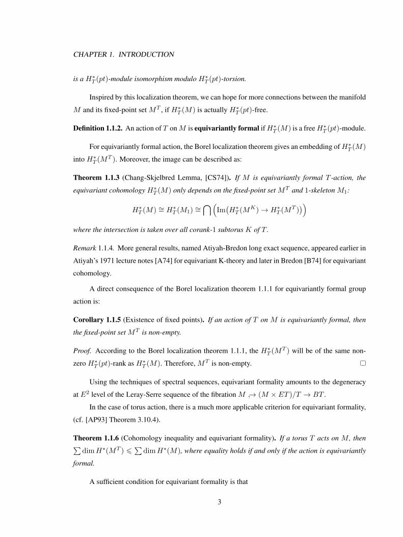
is a H∗T (pt)-module isomorphism modulo H∗T (pt)-torsion.
Inspired by this localization theorem, we can hope for more connections between the manifold
M and its fixed-point set MT , if H∗T (M) is actually H∗T (pt)-free.
Definition 1.1.2. An action of T onM is equivariantly formal ifH∗T (M) is a freeH∗T (pt)-module.
For equivariantly formal action, the Borel localization theorem gives an embedding ofH∗T (M)
into H∗T (MT ). Moreover, the image can be described as:
Theorem 1.1.3 (Chang-Skjelbred Lemma, [CS74]). If M is equivariantly formal T -action, the
equivariant cohomology H∗T (M) only depends on the fixed-point set MT and 1-skeleton M1:
H∗T (M) ∼= H∗T (M1) ∼=⋂(
Im(H∗T (MK)→ H∗T (MT )
))where the intersection is taken over all corank-1 subtorus K of T .
Remark 1.1.4. More general results, named Atiyah-Bredon long exact sequence, appeared earlier in
Atiyah’s 1971 lecture notes [A74] for equivariant K-theory and later in Bredon [B74] for equivariant
cohomology.
A direct consequence of the Borel localization theorem 1.1.1 for equivariantly formal group
action is:
Corollary 1.1.5 (Existence of fixed points). If an action of T on M is equivariantly formal, then
the fixed-point set MT is non-empty.
Proof. According to the Borel localization theorem 1.1.1, the H∗T (MT ) will be of the same non-
zero H∗T (pt)-rank as H∗T (M). Therefore, MT is non-empty.
Using the techniques of spectral sequences, equivariant formality amounts to the degeneracy
at E2 level of the Leray-Serre sequence of the fibration M ↪→ (M × ET )/T → BT .
In the case of torus action, there is a much more applicable criterion for equivariant formality,
(cf. [AP93] Theorem 3.10.4).
Theorem 1.1.6 (Cohomology inequality and equivariant formality). If a torus T acts on M , then∑dimH∗(MT ) 6
∑dimH∗(M), where equality holds if and only if the action is equivariantly
formal.
A sufficient condition for equivariant formality is that
3

CHAPTER 1. INTRODUCTION
Corollary 1.1.7. If a T -manifold M has a T -invariant Morse-Bott function f such that Crit(f) =
MT , then it is equivariantly formal.
Proof. The cohomology H∗(M) can be computed from Morse-Bott-Witten cochain complex gen-
erated on the critical submanifold Crit(f). Hence∑
dimH∗(MT ) =∑
dimH∗(Crit(f)) >∑dimH∗(M). The above theorem 1.1.6 says this inequality is actually an equality and hence the
T -manifold M is equivariantly formal.
Example 1.1.8. When M is equipped with a symplectic form, a Hamiltonian T -action and a mo-
ment map µ : M → t∗, then µξ gives a Morse-Bott function for any generic ξ ∈ t and has
Crit(µξ) = MT , therefore M is T -equivariantly formal.
Restricting to any subtorus K of T acting on M , we get
Proposition 1.1.9 (Inheritance of equivariant formality). An action of torus T onM is equivariantly
formal if and only if for any subtorusK of T , both the sub-action ofK onM and the residual action
of T/K on MK are equivariantly formal.
Proof. Notice that after choosing a subtorus K, the three actions of T on M , K on M and T/K on
MK give us the sequence of inequalities∑dimH∗(MT ) 6
∑dimH∗(MK) 6
∑dimH∗(M)
Thus, we see that the equality∑
dimH∗(MT ) =∑
dimH∗(M) holds if and only if both of
the two intermediate equalities∑
dimH∗(MT ) =∑
dimH∗(MK) and∑
dimH∗(MK) =∑dimH∗(M) hold, which is just a restatement of the proposition.
Combining the Proposition 1.1.9 on inheritance of equivariant formality with the Corollary
1.1.5 on existence of fixed points, we get the inheritance of fixed points:
Corollary 1.1.10 (Inheritance of fixed points). If an action of torus T onM is equivariantly formal,
then for any subtorus K of T , every connected component of MK has T -fixed points.
Proof. By the inheritance of equivariant formality, the residual action of T/K on any connected
component C of MK is also equivariantly formal. Then by the existence of fixed points, CT =
CT/K is non-empty.
4
CHAPTER 1. INTRODUCTION
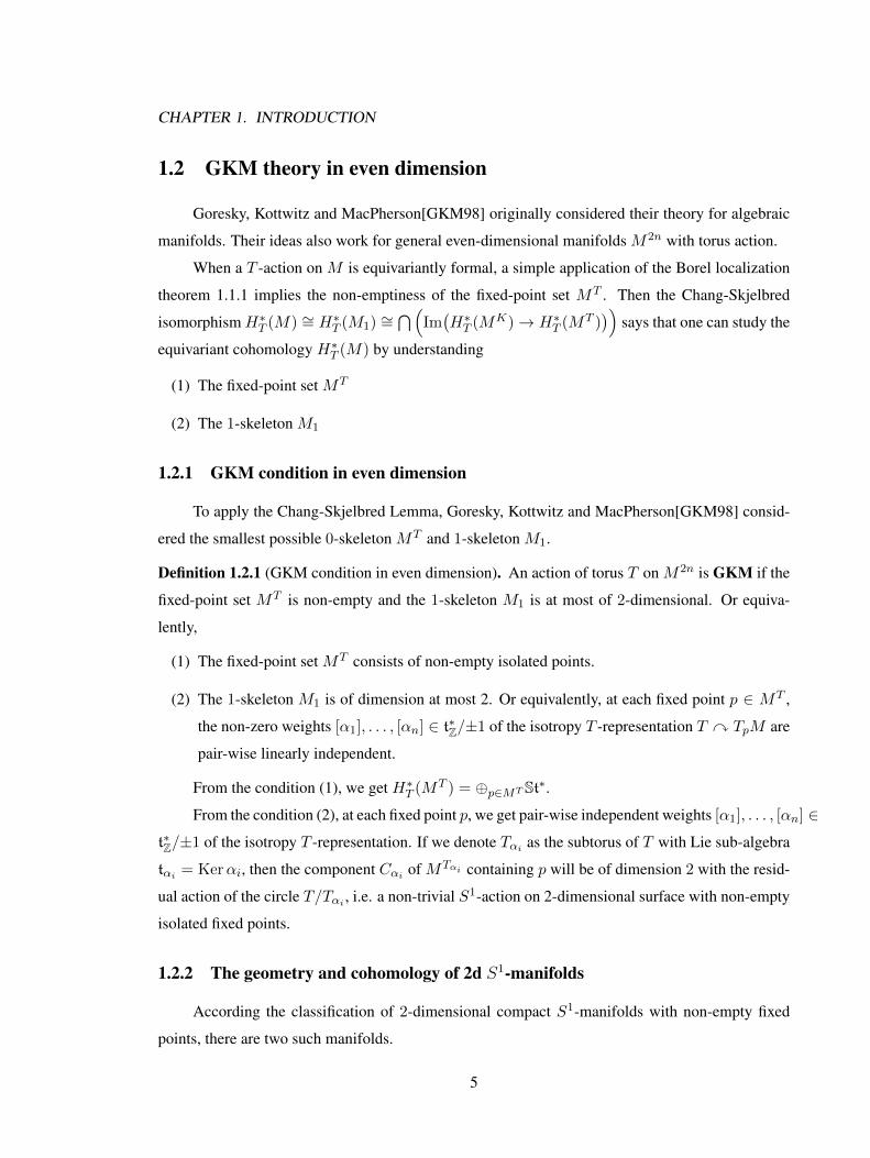
1.2 GKM theory in even dimension
Goresky, Kottwitz and MacPherson[GKM98] originally considered their theory for algebraic
manifolds. Their ideas also work for general even-dimensional manifolds M2n with torus action.
When a T -action on M is equivariantly formal, a simple application of the Borel localization
theorem 1.1.1 implies the non-emptiness of the fixed-point set MT . Then the Chang-Skjelbred
isomorphismH∗T (M) ∼= H∗T (M1) ∼=⋂(
Im(H∗T (MK)→ H∗T (MT )
))says that one can study the
equivariant cohomology H∗T (M) by understanding
(1) The fixed-point set MT
(2) The 1-skeleton M1
1.2.1 GKM condition in even dimension
To apply the Chang-Skjelbred Lemma, Goresky, Kottwitz and MacPherson[GKM98] consid-
ered the smallest possible 0-skeleton MT and 1-skeleton M1.
Definition 1.2.1 (GKM condition in even dimension). An action of torus T on M2n is GKM if the
fixed-point set MT is non-empty and the 1-skeleton M1 is at most of 2-dimensional. Or equiva-
lently,
(1) The fixed-point set MT consists of non-empty isolated points.
(2) The 1-skeleton M1 is of dimension at most 2. Or equivalently, at each fixed point p ∈ MT ,
the non-zero weights [α1], . . . , [αn] ∈ t∗Z/±1 of the isotropy T -representation T y TpM are
pair-wise linearly independent.
From the condition (1), we get H∗T (MT ) = ⊕p∈MT St∗.
From the condition (2), at each fixed point p, we get pair-wise independent weights [α1], . . . , [αn] ∈t∗Z/±1 of the isotropy T -representation. If we denote Tαi as the subtorus of T with Lie sub-algebra
tαi = Kerαi, then the component Cαi of MTαi containing p will be of dimension 2 with the resid-
ual action of the circle T/Tαi , i.e. a non-trivial S1-action on 2-dimensional surface with non-empty
isolated fixed points.
1.2.2 The geometry and cohomology of 2d S1-manifolds
According the classification of 2-dimensional compact S1-manifolds with non-empty fixed
points, there are two such manifolds.
5

CHAPTER 1. INTRODUCTION
Lemma 1.2.2 (see [Au04] subsection I.3.a). If S1 acts effectively on a surface M with non-empty
isolated fixed points, then M is
• S2 with two fixed points
• RP 2 with one fixed point, and an exceptional orbit S1/(Z/2Z)
where RP 2 as the Z/2Z quotient of S2, has the induced S1-action from S2.
Using equivariant Mayer-Vietoris sequence, we see that the S1-actions on S2 and RP 2 are
both equivariantly formal, with equivariant cohomology
H∗S1(S2) ={
(fN , fS) ∈ Q[u]⊕Q[u] | fN (0) = fS(0)}
H∗S1(RP 2) = Q[u]
Transferring to the T -action on S2 or RP 2 with subtorus Tα acting trivially and the residual
circle T/Tα-action equivariantly formal, the equivariant cohomology is
H∗T (S2[α]) = H∗T/Tα(S2
[α])⊗H∗Tα(pt)
={
(fN , fS) ∈ St∗ ⊕ St∗ | fN ≡ fS mod α}
H∗T (RP 2[α]) = St∗
giving relations of elements of H∗T (M) expressed in terms of H∗T (MT ).
1.2.3 The GKM graph and GKM theorem in even dimension
In the 1-skeleton M1, each S2 has two fixed points, and each RP 2 has one fixed point. This
observation leads to a graphic representation of the relation among MT and M1.
Definition 1.2.3 (GKM graph in even dimension). The GKM graph of a GKM action of torus T
on M2n consists of
Vertices There are two types of vertices
• for each fixed point in MT
Empty dot for each RP 2 ∈M1
Edges & Weights A solid edge with weight [α] for each S1[α] joining two •’s representing its two
fixed points, and a dotted edge with weight [β] for each RP 2[β] joining a • to an empty dot.
6
CHAPTER 1. INTRODUCTION
Remark 1.2.4. The GKM graphs were originally defined for orientable even-dimensional manifolds
and hence only have one type of vertices. The above GKM graph with two type of vertices for
possibly non-orientable even-dimensional manifolds are due to Goertsches and Mare [GM14].
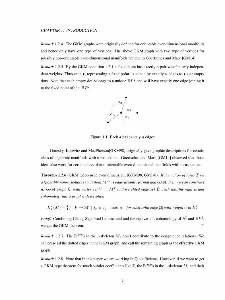
Remark 1.2.5. By the GKM condition 1.2.1, a fixed point has exactly n pair-wise linearly indepen-
dent weights. Thus each •, representing a fixed point, is joined by exactly n edges to •’s or empty
dots. Note that each empty dot belongs to a unique RP 2 and will have exactly one edge joining it
to the fixed point of that RP 2.
α1
α2
αn−1αn
Figure 1.1: Each • has exactly n edges
Goresky, Kottwitz and MacPherson[GKM98] originally gave graphic descriptions for certain
class of algebraic manifolds with torus actions. Goertsches and Mare [GM14] observed that those
ideas also work for certain class of non-orientable even-dimensional manifolds with torus action.
Theorem 1.2.6 (GKM theorem in even dimension, [GKM98, GM14]). If the action of torus T on
a (possibly non-orientable) manifold M2n is equivariantly formal and GKM, then we can construct
its GKM graph G, with vertex set V = MT and weighted edge set E, such that the equivariant
cohomology has a graphic description
H∗T (M) ={f : V → St∗ | fp ≡ fq mod α for each solid edge pq with weight α in E
}Proof. Combining Chang-Skjelbred Lemma and and the equivariant cohomology of S2 and RP 2,
we get the GKM theorem.
Remark 1.2.7. The RP 2’s in the 1-skeleton M1 don’t contribute to the congruence relations. We
can erase all the dotted edges in the GKM graph, and call the remaining graph as the effective GKM
graph.
Remark 1.2.8. Note that in this paper we are working in Q coefficients. However, if we want to get
a GKM-type theorem for much subtler coefficients like Z, the RP 2’s in the 1-skeleton M1 and their
7
CHAPTER 1. INTRODUCTION
corresponding dotted edges in the GKM graph are as crucial as the S2’s and their corresponding
solid edges.
Remark 1.2.9. If M2n has a T -invariant stable almost complex structure, then the isotropy weights
α1, . . . , αn ∈ t∗Z are determined with signs, and its GKM graph can be made into a directed graph.
Moreover, as explained by Guillemin and Zara [GZ01], there is a set of congruence relations be-
tween the bouquets of isotropy weights for each edge, and they call it the connection of the GKM
graph.
Remark 1.2.10. We have assumed M to be connected. Suppose its GKM graph G has l connected
components G1, . . . ,Gl. Note the assignment of polynomials on vertices from the same Gi with the
same constant rational number gives all the elements in the graphic description of H0T (M). Thus
we have dimH0T (M) = l = 1, i.e. the graph G is also connected.
Example 1.2.11. Toric manifolds are GKM manifolds.
Example 1.2.12. For the sphere S2n, we use the coordinates (x, z1, . . . , zn) where x is a real
variable, zi’s are complex variables. Let Tn act on S2n by (eiθ1 , . . . , eiθn) · (x, z1, . . . , zn) =
(x, eiθ1z1, . . . , eiθnzn) with fixed-point set (S2n)T
n= {(±1, 0, . . . , 0)}. Since dimH∗((S2n)T
n) =
2 = dimH∗(S2n), the Tn action on S2n is equivariantly formal by the formality criterion Theorem
1.1.6. Let α1, . . . , αn be the standard integral basis of t∗Z = Zn, then each fixed point has the un-
signed isotropy weights [α1], . . . , [αn]. This means the action is GKM and the GKM graph consists
of two vertices with n edges weighted [α1], . . . , [αn] joining them. The equivariant cohomology is
then H∗Tn(S2n) = {(f, g) ∈ St∗ ⊕ St∗ | f ≡ g mod∏ni=1 αi}.
Example 1.2.13. RP 2n as the quotient of S2n by the Z/2Z action eπi·(x, z1, . . . , zn) = (−x,−z1, . . . ,−zn)
also inherits a Tn-action from that on S2n, discussed in previous section. The fixed-point set
is (RP 2n)Tn
= {(±1, 0, . . . , 0)}/(Z/2Z), a single point. Since dimH∗((RP 2n)Tn) = 1 =
dimH∗(RP 2n), the Tn action on RP 2n is equivariantly formal by the formality criterion Theo-
rem 1.1.6 with the unsigned isotropy weights [α1], . . . , [αn] at the only fixed point. This means
the action is GKM and the GKM graph consists of a single vertex with n dotted edges weighted
[α1], . . . , [αn], and the effective GKM graph is a single vertex without edges. The equivariant co-
homology is then H∗Tn(RP 2n) = St∗.
Example 1.2.14. Let’s consider the real Grassmannian G2k(R2n). Write the coordinates on R2n
as (x1, y1, . . . , xn, yn). Let Tn act on R2n so that the i-th S1-component of Tn exactly rotates the
i-th pairs of real coordinates (xi, yi) and leaves the remaining coordinates free, hence we can write
8
CHAPTER 1. INTRODUCTION
R2n = ⊕ni=1R2[αi]
for their decompositions into weighted subspaces, where [αi] ∈ t∗Z/ ± 1. These
actions induce Tn actions on G2k(R2n). In order to determine the fixed-point set and 1-skeleton
of the action Tn y G2k(R2n), we only need to observe that fixed-points of Tn y G2k(R2n) are
exactly the Tn-subrepresentations of R2n = ⊕ni=1R2[αi]
. It’s not hard to show that the GKM graph
of Tn y G2k(R2n) consists of
Vertices G2k(R2n)Tn ∼=
{S ⊆ {1, 2, . . . , n} | #S = k
}Edges If S\{i} = S′\{j}, then there are two edges with weights [αj−αi] and [αj+αi] connecting
S and S′
Denote S = G2k(R2n)Tn
as the collection of k-element subset of {1, 2, . . . , n}. Then the GKM
description then can be given as the following collection of maps:{f : S → Q[α1, . . . , αn] | fS ≡ fS′ mod α2
j − α2i for S\{i} = S′\{j}
}Example 1.2.15. Let M2n → M2n be a T -equivariant finite covering with deck transformation
group Γ. If the T -action on M is equivariantly formal and GKM, then according to the even-
dimensional GKM theorem 1.2.6, the equivariant cohomology H∗T (M) concentrates on even de-
grees, so does its ordinary cohomologyH∗(M). SinceH∗(M) ∼= H∗(M)Γ, the ordinary cohomol-
ogy H∗(M) also concentrates on even degrees, which means the T -action on M is equivariantly
formal. The isotropy weights at T -fixed points of M are inherited from M , hence T -action on M is
also GKM. Restricting the covering to fixed points and 1-skeleta MT → MT , M1 → M1 and de-
noting G, G as the GKM graphs of M, M , we can view the GKM graph G as G/Γ in the following
sense: the Γ-orbits of • vertices in G one-to-one correspond to the • vertices in G; the free Γ-orbits
of solid edges in G one-to-one correspond to solid edges in G; the Γ-orbits of empty vertices and
dotted edges in G form part of the empty vertices and dotted edges in G; the non-free Γ-orbits of
solid edges in G form the remaining empty vertices and dotted edges in G.
Example 1.2.16. As an application, we can revisit Guillemin, Holm and Zara’s [GHZ06] GKM
description of homogeneous space G/K where rankG = rankK and K is connected. We can
actually drop the assumption of K being connected. Let K0 be the identity component of K and
fix a maximal torus T of K0. Under the left action of T , both G/K0 and G/K are equivariantly
formal and GKM with GKM graphs denoted as GG/K0, GG/K . Note the coveringG/K0 → G/K is
T -equivariant with deck transformation group K/K0, we get the relation between the GKM graphs
as GG/K = GG/K0/(K/K0).
9
CHAPTER 1. INTRODUCTION
Remark 1.2.17. Besides the application to covering spaces, the even-dimensional GKM theorem
1.2.6 for possibly non-orientable manifolds can also be readily applied to related fibrations devel-
oped by Guillemin, Sabatini and Zara [GSZ12].
1.3 S1-actions on closed 3d manifolds
The idea of classifying effective S1-actions in dimension 3 is the same as in dimension 2 by
listing all the possible equivariant tubular neighbourhoods of non-principal orbits, and then try to
patch them together. But one more dimension for the isotropic representations provides a longer list
of equivariant tubular neighbourhoods.
1.3.1 Equivariant tubular neighbourhoods of principal orbits
For a point x of principal type, its isotropy group is the identity group {1} with a trivial
isotropic representation {1} y R2. So an equivariant tubular neighbourhood of S1 · x can be
written as S1 ×{1} D = S1 × D, with the S1-action concentrating entirely on the S1-factor. So
the orbit space of this tubular neighbourhood is (S1 ×D)/S1 = S1/S1 ×D = D, a smooth local
chart.
1.3.2 Equivariant tubular neighbourhoods of exceptional orbits
The union of exceptional orbits will be denoted as E. For an exceptional orbit S1/Zm with
stabilizer Zm = {e2πkim , k = 1, 2, . . . ,m}, its isotropic representation of Zm is 2-dimensional. Such
a 2-dimensional effective Zm-representation could preserve the orientation by rotating:
Zmrotatey C : e
2πkim ◦ z = (e
2πkim )nz
where the orbit invariants (m, n), also called Seifert invariants, are coprime positive integers, and
0 < n < m. The resulting equivariant tubular neighbourhood is S1×Zm D, whose orbit space is an
orbifold disk
(S1 ×Zm D)/S1 = D/Zm
where the central orbifold point pt/Zm corresponds to the exceptional orbit S1/Zm.
10
CHAPTER 1. INTRODUCTION
1.3.3 Equivariant tubular neighbourhoods of special exceptional orbits
Besides rotating, a 2-dimensional effective Zm-representation could also reverse the orienta-
tion by reflection:
Z2reflecty R2 : eπi ◦ (x, y) = (−x, y)
This case requires the Zm to be Z2. Because of the reverse of orientation, we call such an orbit
S1/Z2 a special exceptional orbit. The union of all such special exceptional orbits will be denoted
as SE.
If we use the open square I × I = {(x, y) | −1 < x, y < 1} as a neighbourhood in R2, an
equivariant tubular neighbourhood of the special exceptional orbit S1/Z2 can be written as S1 ×Z2
(I×I), the orbit space by Z2 of the solid torus S1×(I×I). Note that the reflection Z2reflecty I×I :
eπi ◦ (x, y) = (−x, y) only affects the first I-factor, so we can split the second I-factor out of the
orbit space S1 ×Z2 (I × I):
S1 ×Z2 (I × I) = S1 × (I × I)/(eiθ, x, y) ∼ (−eiθ,−x, y)
=(S1 × I/(eiθ, x) ∼ (−eiθ,−x)
)× I = Mob× I
where we write Mob for short of the Mobius band S1 ×Z2 I .
Because the set of points with stabilizer Z2 in the Mobius band S1×Z2 I is Mob(Z2) = S1×Z2
{0} = S1/Z2 a circle, the set of points with stabilizer Z2 in Mob×I is (Mob×I)(Z2) = S1/Z2×Iof dimension 2. Thus, if a 3d S1-manifold M has a special exceptional orbit S1/Z2, then the
connected component of M(Z2) that contains this orbit will be of dimension 2 and is acted freely by
S1/Z2, hence has to be S1/Z2 × S1 according the list of 2d S1-manifolds.
Now an equivariant tubular neighbourhood of this torus S1/Z2×S1 will be a bundle of Mobius
band over S1, which is actually a product bundle Mob× S1, cf. Raymond [Ra68].
Notice that the S1-action concentrates entirely on the factor of Mobius band, so the orbit space
is (Mob× I)/S1 = Mob/S1 × I = [0, 1)× I with a boundary circle {0} × S1.
1.3.4 Equivariant tubular neighbourhoods of fixed points
The set of fixed points will be denoted as F . For a fixed point x with stabilizer S1, its isotropic
representation is of dimension 3. There is only one such effective 3-dimensional S1-representation
S1 y C⊕ R by acting on the C-factor rotationally and acting on the R-factor trivially.
So an equivariant tubular neighbourhood of x can be written as D × I , with fixed point set
{0} × I , an interval. We can continue to glue along this fixed interval to form S1, a connected
11
CHAPTER 1. INTRODUCTION
component of the fixed point set. Now an enlarged equivariant tubular neighbourhood of the fixed
circle S1 is going to be a disk bundle over the S1, which is actually a product bundle D × S1, cf.
Raymond [Ra68].
Notice that the S1-action concentrates entirely on the D-factor, so the orbit space is (D ×S1)/S1 = D/S1 × S1 = [0, 1)× S1 with a boundary circle {0} × S1.
1.3.5 Patching: from local to global
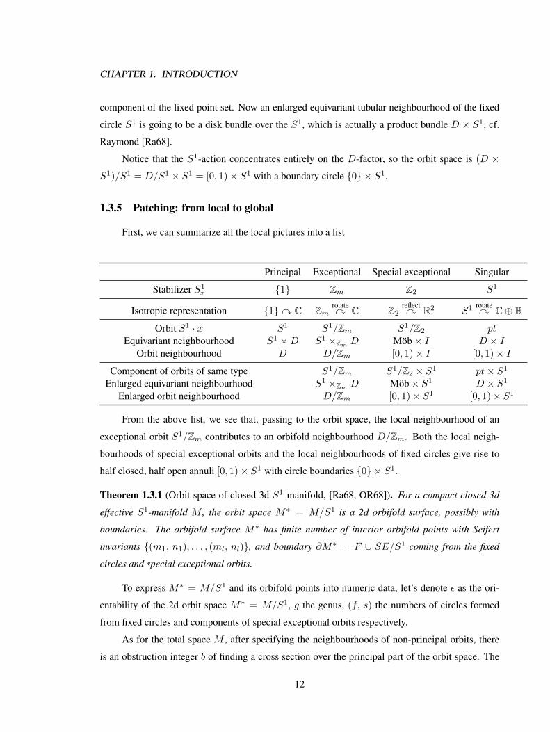
First, we can summarize all the local pictures into a list
Principal Exceptional Special exceptional Singular
Stabilizer S1x {1} Zm Z2 S1
Isotropic representation {1}y C Zmrotatey C Z2
reflecty R2 S1 rotatey C⊕ R
Orbit S1 · x S1 S1/Zm S1/Z2 ptEquivariant neighbourhood S1 ×D S1 ×Zm D Mob× I D × I
Orbit neighbourhood D D/Zm [0, 1)× I [0, 1)× I
Component of orbits of same type S1/Zm S1/Z2 × S1 pt× S1
Enlarged equivariant neighbourhood S1 ×Zm D Mob× S1 D × S1
Enlarged orbit neighbourhood D/Zm [0, 1)× S1 [0, 1)× S1
From the above list, we see that, passing to the orbit space, the local neighbourhood of an
exceptional orbit S1/Zm contributes to an orbifold neighbourhood D/Zm. Both the local neigh-
bourhoods of special exceptional orbits and the local neighbourhoods of fixed circles give rise to
half closed, half open annuli [0, 1)× S1 with circle boundaries {0} × S1.
Theorem 1.3.1 (Orbit space of closed 3d S1-manifold, [Ra68, OR68]). For a compact closed 3d
effective S1-manifold M , the orbit space M∗ = M/S1 is a 2d orbifold surface, possibly with
boundaries. The orbifold surface M∗ has finite number of interior orbifold points with Seifert
invariants {(m1, n1), . . . , (ml, nl)}, and boundary ∂M∗ = F ∪ SE/S1 coming from the fixed
circles and special exceptional orbits.
To express M∗ = M/S1 and its orbifold points into numeric data, let’s denote ε as the ori-
entability of the 2d orbit space M∗ = M/S1, g the genus, (f, s) the numbers of circles formed
from fixed circles and components of special exceptional orbits respectively.
As for the total space M , after specifying the neighbourhoods of non-principal orbits, there
is an obstruction integer b of finding a cross section over the principal part of the orbit space. The
12
CHAPTER 1. INTRODUCTION
theorem by Orlik and Raymond says that, these invariants completely classify the 3d S1-manifolds,
after adding some constraints within these invariants. The following version is taken from Orlik’s
lecture notes [Or72].
Theorem 1.3.2 (Equivariant classification of closed 3d S1-manifolds, [Ra68, OR68]). Let S1 act
effectively and smoothly on a closed, connected smooth 3d manifold M . Then the orbit invariants
{b; (ε, g, f, s); (m1, n1), . . . , (ml, nl)
}determine M up to equivariant diffeomorphisms, subject to the following conditions
(1) b = 0, if f + s > 0
b ∈ Z, if f + s = 0 and ε = o, orientable
b ∈ Z2, if f + s = 0 and ε = n, non-orientable
b = 0, if f + s = 0, ε = n and mi = 2 for some i
(2) 0 < ni < mi, (mi, ni) = 1 if ε = o
0 < ni 6mi2 , (mi, ni) = 1 if ε = n
Conversely, any such set of invariants can be realized as a closed 3d manifold with an effective
S1-action.
Remark 1.3.3. Raymond’s idea of proving this classification theorem is as follows: given any two
closed 3d S1-manifolds M,M with the same orbit invariants, firstly we can establish an orbifold
diffeomorphism between M/S1 and M/S1. Secondly, we can lift this orbifold diffeomorphism to
E ∪ F ∪ SE → E ∪ F ∪ SE between the three types of non-principal orbits and extend this map
to a tubular neighbourhood of the non-principal orbits. Finally, we can extend this map to all the
principal orbits using local cross sections, which actually gives a global S1-diffeomorphism if the
principal Euler numbers b, b are the same.
Remark 1.3.4. When M has neither fixed point nor special exceptional orbit, i.e. f = s = 0, then
this is the case of Seifert manifolds.
Remark 1.3.5. The invariants in M ={b; (ε, g, f, s); (m1, n1), . . . , (ml, nl)
}mostly come from
the orbit space M∗ = M/S1 except the invariant b. Therefore the constraint (b = 0, if f + s > 0)
says that if the orbifoldM∗ has boundaries, thenM ={b = 0; (ε, g, f, s); (m1, n1), . . . , (ml, nl)
}is determined by the orbifold M/S1 and the assignment of its boundary circles being either from
fixed components or special exceptional components.
13
CHAPTER 1. INTRODUCTION
Remark 1.3.6. The above classification is up to equivariant diffeomorphisms. But Orlik and Ray-
mond also discussed in certain conditions, more than one S1-actions can appear on the same 3d
manifold.
For an orientable S1-manifold M , the orbit space M∗ = M/S1 will be orientable, i.e. ε = o,
and there will be no special exceptional orbits, i.e. s = 0.
Corollary 1.3.7 (Classification of closed orientable 3d S1-manifolds, [Ra68, OR68]). If a closed
3d S1-manifold is oriented and the S1-action preserves the orientation. Then the orbit invariants
{b; (ε = o, g, f, s = 0); (m1, n1), . . . , (ml, nl)
}determine M up to equivariant diffeomorphisms, subject to the following conditions
(1) b = 0, if f > 0
b ∈ Z, if f = 0
(2) 0 < ni < mi, (mi, ni) = 1
14
Chapter 2
Equivariant cohomology of 3d
S1-manifolds
The classification of 3d S1-manifolds (possibly with boundaries) in terms of numeric invari-
ants and graphs gives us an S1-equivariant stratification of every such manifold and enables us to
calculate all kinds of topological data. For example, the fundamental groups, ordinary cohomology
with Z or Zp coefficients have been computed extensively for closed 3d S1-manifolds in literature
[JN83, BZ03], and now can be generalized to 3d S1-manifolds with boundaries, using the classifi-
cation Theorems 1.3.2. But not much has been discussed for S1-equivariant cohomology, which is
the goal of current section.
In the following subsections, we will first prove our core Theorem 2.2.5 in full generality.
When we explore more delicate computational invariants, we will try to keep the presentation of
results in a manageable way but perhaps with a slight loss of generality.
2.1 More basic facts about equivariant cohomology
In the following discussion, the coefficient of cohomology will always be Q unless otherwise
mentioned. For a group action of G on M , the equivariant cohomology ring is defined using the
Borel constructionH∗G(M) = H∗(EG×GM), whereH∗(−) is the ordinary simplicial cohomology
theory, EG is the universal principal G-bundle and EG ×G M is the associated bundle with fibre
M . The pull-back π∗ : H∗G(pt) −→ H∗G(M) of the trivial map π : M −→ pt gives H∗G(M) a
module structure of the ring H∗G(pt).
15
CHAPTER 2. EQUIVARIANT COHOMOLOGY OF 3D S1-MANIFOLDS
In general, the equivariant cohomology H∗G(M) is not the same as the ordinary cohomology
H∗(M/G) of the orbit space M/G. If we choose any fibre inclusion ι : M → EG ×M and pass
to the orbit spaces ι : M/G→ EG×GM , then the pull-back ι∗ : H∗G(M) = H∗(EG×GM)→H∗(M/G) gives a natural map between H∗G(M) and H∗(M/G).
We will need some basic facts to compute equivariant cohomology, see the expository survey
[Go] for details.
The first set of facts is about equivariant cohomology of homogeneous space, i.e. space with
one single orbit:
Fact 2.1.1. Let G be a compact Lie group, and H a closed Lie subgroup. Denote BG = EG/G
and BH = EH/H for the classifying space of G-bundles and H-bundles respectively. Then,
• H∗G(pt) = H∗(EG/G) = H∗(BG)
• H∗G(G/H) ∼= H∗H(pt) = H∗(BH)
The second set of facts is about equivariant cohomology of extremal types of group actions:
Fact 2.1.2. Let a compact Lie group G act on a compact manifold M .
• If the action GyM is free, then H∗G(M) ∼= H∗(M/G).
• If the action GyM is trivial, then H∗G(M) ∼= H∗(M)⊗H∗G(pt).
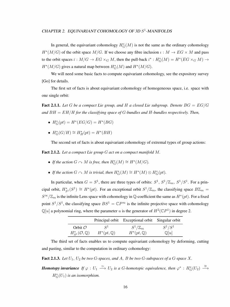
In particular, when G = S1, there are three types of orbits: S1, S1/Zm, S1/S1. For a prin-
cipal orbit, H∗S1(S1) ∼= H∗(pt). For an exceptional orbit S1/Zm, the classifying space BZm =
S∞/Zm is the infinite Lens space with cohomology in Q-coefficient the same asH∗(pt). For a fixed
point S1/S1, the classifying space BS1 = CP∞ is the infinite projective space with cohomology
Q[u] a polynomial ring, where the parameter u is the generator of H2(CP 1) in degree 2.
Principal orbit Exceptional orbit Singular orbit
Orbit O S1 S1/Zm S1/S1
H∗S1(O,Q) H∗(pt,Q) H∗(pt,Q) Q[u]
The third set of facts enables us to compute equivariant cohomology by deforming, cutting
and pasting, similar to the computation in ordinary cohomology:
Fact 2.1.3. Let U1, U2 be two G-spaces, and A, B be two G-subspaces of a G-space X .
Homotopy invariance If ϕ : U1'−→ U2 is a G-homotopic equivalence, then ϕ∗ : H∗G(U2)
∼=−→H∗G(U1) is an isomorphism.
16

CHAPTER 2. EQUIVARIANT COHOMOLOGY OF 3D S1-MANIFOLDS
Mayer-Vietoris sequence If X = A◦ ∪B◦ is the union of interiors of A and B, then there is a long
exact sequence:
· · · −→ H iG(X) −→ H i
G(A)⊕H iG(B) −→ H i
G(A ∩B)δ−→ H i+1
G (X) −→ · · ·
Remark 2.1.4. Besides the Borel model of equivariant cohomology, there are also Cartan model
and Weil model (cf. Guillemin-Sternberg [GS99]) using equivariant de Rham theory. In this paper,
we prefer the Borel model because the homotopy invariance and Mayer-Vietoris sequence are more
natural for Borel model, from the topological rather than the differential point of view.
The fourth set of facts deals with equivariant cohomology of product spaces:
Fact 2.1.5. Let G y M and H y N be two group actions on manifolds. Then, for the product
action G×H yM ×N , we get
H∗G×H(M ×N) ∼= H∗G(M)⊗H∗H(N)
Especially, for the action GyM ×N where N is acted by G trivially, we get
H∗G(M ×N) ∼= H∗G(M)⊗H∗(N)
2.2 A short exact sequence
Let S1 act effectively on a compact connected 3d manifold M , possibly with boundary. We
will compute the equivariant cohomology group H∗S1(M,Q) by cutting and pasting, with the help
of the classification theorem from previous sections.
As we have seen from the previous computation of H∗S1(O) for each S1-orbit O, the S1-
equivariant cohomology in Q coefficient does not distinguish principal orbit S1 from exceptional
orbit S1/Zm or special exceptional orbit S1/Z2. However, there is big difference between the
S1-equivariant cohomology of fixed point and non-fixed orbit.
If a 3d S1-manifold M does not have fixed points, we would hope that its S1-equivariant co-
homology is the ordinary cohomology of the orbit space M/S1. Actually, a more general statement
is true due to Satake [Sa56]. The version here is taken from Duistermaat’s lecture notes [Du94].
Definition 2.2.1. An action of a compact Lie group G on a manifold M is locally free, if for every
x ∈M , the isotropy group Gx is finite.
17

CHAPTER 2. EQUIVARIANT COHOMOLOGY OF 3D S1-MANIFOLDS
Theorem 2.2.2 (Satake [Sa56]). If a compact Lie groupG acts locally freely on a compact manifold
M , then M/G is an orbifold, and H∗G(M,R) ∼= H∗(M/G,R).
We can certainly apply the Theorem of Satake to our special case of S1-actions. However,
there is a subtlety in Satake’s definition ofH∗(M/S1,R) for the orbifoldM/S1 in terms of orbifold
differential forms (cf. [Sa56, Du94]). Moreover, because of the use of differential forms, the above
theorem is originally stated for R-coefficients not for Q-coefficients.
In our definition ofH∗(M/S1,Q), we will simply use the ordinary simplicial cohomology for
the topological space M/S1 by forgetting its orbifold structure.
Our method of calculating equivariant cohomology is based on the equivariant Meyer-Vietoris
sequence and induction on the number of non-principal components which is finite because of the
compactness of M .
Proposition 2.2.3. Let S1 act effectively on a compact connected 3d manifold M , possibly with
boundary. If M does not have fixed points, then H∗S1(M,Q) ∼= H∗(M/S1,Q).
Proof. We will proceed by induction on the number of non-principal components.
To begin with, suppose M does not have non-principal component. Since we assume there is
no fixed point, then S1 acts on M freely and hence H∗S1(M) ∼= H∗(M/S1).
Now suppose the proposition is true for any 3d fixed-point-free S1-manifold with k > 0
non-principal components, and suppose M has k + 1 non-principal components. Let C be a non-
principal component together with an equivariant tubular neighbourhood N , then the complement
M ′ = M r N has k non-principal components and H∗S1(M ′) ∼= H∗(M ′/S1) according to our
assumption. Let’s also denote L = M ′ ∩NThe equivariant Mayer-Vietoris sequence for the unionM = M ′∪N and the ordinary Mayer-
Vietoris sequence for the union M/S1 = M ′/S1 ∪N/S1 gives:
H∗−1S1 (M ′)⊕H∗−1
S1 (N) H∗−1S1 (L) H∗S1(M) H∗S1(M ′)⊕H∗S1(N) H∗S1(L)
H∗−1(M ′/S1)⊕H∗−1(N/S1) H∗−1(L/S1) H∗(M/S1) H∗(M ′/S1)⊕H∗(N/S1) H∗(L/S1)
where the second and the fifth vertical maps are isomorphisms, because the intersectionL = M ′∩Ndoes not touch non-principal orbits and consists of only principal orbits.
According to the Five Lemma in homological algebra, in order to prove that the middle vertical
map is an isomorphism, we now need to prove the first and the fourth maps are isomorphisms. But
18

CHAPTER 2. EQUIVARIANT COHOMOLOGY OF 3D S1-MANIFOLDS
we already have the isomorphism H∗S1(M ′) ∼= H∗(M ′/S1). So we only need to prove H∗S1(N) ∼=H∗(N/S1).
For a 3d fixed-point-free S1-manifold M , according to our detailed discussion in Section 1.3,
there are three cases for a non-fixed, non-principal component C, its equivariant neighbourhood
N and orbit space N/S1. Note that, for each case, there is an equivariant deformation retraction
N ' C, so we have H∗S1(N) ∼= H∗S1(C). Also recall that we have calculated H∗S1(S1/Zm,Q) ∼=H∗(pt,Q).
C S1/Zm S1/Z2 × S1
N S1 ×Zm D2 Mob× S1
N/S1 D2/Zm I × S1
H∗S1(N) ∼= H∗S1(C) H∗(pt) H∗(S1)
H∗(N/S1) H∗(D2/Zm) H∗(S1)
For the second and the third case, it is clear that H∗S1(N) ∼= H∗(N/S1). For the first case, the
orbit space D2/Zm, viewed as an ice-cream cone, has a deformation retract to the cone’s tip pt, so
H∗S1(N) ∼= H∗(pt) ∼= H∗(D2/Zm) = H∗(N/S1).
If a 3d S1-manifold M has fixed points, then the number of fixed components will be finite
due to the compactness of M , and every fixed component is a circle S1 according to our discussion
in the previous Subsection 1.3.4. The calculation of S1 equivariant cohomology of a general 3d
S1-manifold M will be carried out by doing induction on the number of connected components of
these fixed points. The beginning case of no fixed points is just the previous Proposition 2.2.3.
Suppose now that an S1-manifold M has k > 0 connected components of fixed points. Let’s
choose any such connected component F , with its equivariant neighbourhood N . According to
Subsection 1.3.4, we have N = D × F . If we set the complement M ′ = M r N , then M is
attached equivariantly by M ′ and N = D × F along S1 × F . The Mayer-Vietoris sequence of
equivariant cohomology groups then gives
→ H∗S1(M,Q)→ H∗S1(M ′,Q)⊕H∗S1(D × F,Q)→ H∗S1(S1 × F,Q)→ H∗+1S1 (M,Q)→
However, since the S1-action on D× F and S1 × F concentrates on their first components respec-
tively, we have:
19

CHAPTER 2. EQUIVARIANT COHOMOLOGY OF 3D S1-MANIFOLDS
H∗S1(D × F ) H∗S1(S1 × F )
H∗S1(D)⊗H∗(F ) H∗S1(S1)⊗H∗(F )
Q[u]⊗H∗(F ) H∗(F ) : f(u)⊗ α f(0) · α
where the upper 2 vertical isomorphisms are because of the cohomology of product spaces, the
lower left vertical isomorphism is because of homotopy between D and pt, and the lower right
vertical isomorphism is because the S1 is a principal orbit.
The bottom map is obviously surjective, so is the top mapH∗S1(D×F )→ H∗S1(S1×F ). This
means that the long exact sequence actually stops atH∗S1(M ′)⊕H∗S1(D×F )→ H∗S1(S1×F )→ 0.
We then conclude that the long exact sequence reduces into the following short exact sequence:
0→ H∗S1(M)→ H∗S1(M ′)⊕(Q[u]⊗H∗(F )
)→ H∗(F )→ 0
where we have replaced the H∗S1(D× F ) and H∗S1(S1 × F ) by Q[u]⊗H∗(F ) and H∗(F ) respec-
tively.
We can now consider all the k components of fixed points F1, F2, . . . , Fk, together with their
equivariant tubular neighbourhood N1, N2, . . . , Nk. If we set the complement M◦ = M r ∪iNi,
an S1-manifold without fixed points, then there is a short exact sequence of cohomology groups:
0→ H∗S1(M)→ H∗S1(M◦)⊕⊕i(Q[u]⊗H∗(Fi)
)→ ⊕iH∗(Fi)→ 0 (†)
Since M◦ is fixed-point-free, H∗S1(M◦,Q) ∼= H∗(M◦/S1,Q) by Proposition 2.2.3. To under-
stand the orbit space M◦/S1, we can compare it with the orbit space M/S1.
Lemma 2.2.4. Following the above notation, the two orbit spaces M◦/S1 and M/S1 are topolog-
ically homotopic. Especially, H∗(M◦/S1,Q) ∼= H∗(M/S1,Q).
Proof. Since the majority ofM◦/S1 andM/S1 is isomorphic, we only need to check what happens
in an equivariant neighbourhood N near an S1-fixed component F of M .
Let N ′ be an equivariant neighbourhood slightly larger than N . If we choose local S1-
equivariant coordinates properly, we can write N ′ = D1 × F and N = D 12× F , where D1
andD 12
are 2-dimensional disks of radii 1 and 12 , such that S1 acts on the disks by standard rotation.
20
CHAPTER 2. EQUIVARIANT COHOMOLOGY OF 3D S1-MANIFOLDS
Now N ′ r N = (D1 r D 12) × F and N ′ = D1 × F are equivariant neighbourhoods of
M◦ = M r N and M respectively. Their orbit spaces by the S1-action give neighbourhoods
(N ′ rN)/S1 and N ′/S1 of M◦/S1 and M/S1 respectively.
However,
(N ′ rN)/S1 =(
(D1 rD 12)/S1
)× F = [
1
2, 1)× F
and
N ′/S1 =(D1/S
1)× F = [0, 1)× F
are homotopic. Thus M◦/S1 and M/S1 are homotopic.
Finally, we can combine all the above discussions and get:
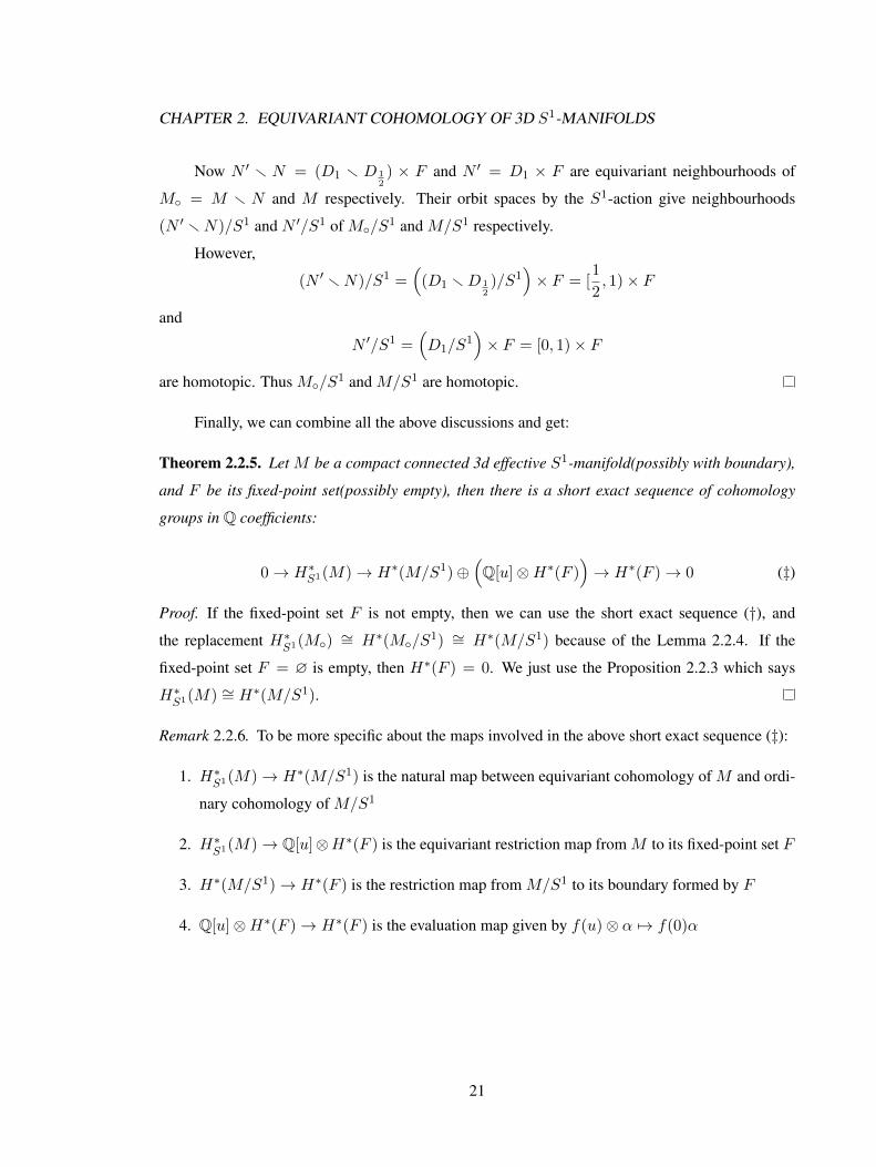
Theorem 2.2.5. Let M be a compact connected 3d effective S1-manifold(possibly with boundary),
and F be its fixed-point set(possibly empty), then there is a short exact sequence of cohomology
groups in Q coefficients:
0→ H∗S1(M)→ H∗(M/S1)⊕(Q[u]⊗H∗(F )
)→ H∗(F )→ 0 (‡)
Proof. If the fixed-point set F is not empty, then we can use the short exact sequence (†), and
the replacement H∗S1(M◦) ∼= H∗(M◦/S1) ∼= H∗(M/S1) because of the Lemma 2.2.4. If the
fixed-point set F = ∅ is empty, then H∗(F ) = 0. We just use the Proposition 2.2.3 which says
H∗S1(M) ∼= H∗(M/S1).
Remark 2.2.6. To be more specific about the maps involved in the above short exact sequence (‡):
1. H∗S1(M)→ H∗(M/S1) is the natural map between equivariant cohomology of M and ordi-
nary cohomology of M/S1
2. H∗S1(M)→ Q[u]⊗H∗(F ) is the equivariant restriction map from M to its fixed-point set F
3. H∗(M/S1)→ H∗(F ) is the restriction map from M/S1 to its boundary formed by F
4. Q[u]⊗H∗(F )→ H∗(F ) is the evaluation map given by f(u)⊗ α 7→ f(0)α
21
CHAPTER 2. EQUIVARIANT COHOMOLOGY OF 3D S1-MANIFOLDS
2.3 The ring and module structure
By the short exact sequence (‡) of Theorem 2.2.5, we have the inclusion of cohomology
groups: H∗S1(M) ↪→ H∗(M/S1) ⊕(Q[u] ⊗ H∗(F )
). Since this inclusion is the direct sum of
two restriction maps of cohomology rings, it preserves ring structure. Therefore, we can describe
the ring structure of H∗S1(M) explicitly in terms of elements and constraints in H∗(M/S1) and
Q[u]⊗H∗(F ).
For simplicity, we will focus on closed 3d S1-manifolds. IfM does not have fixed points, then
the Proposition 2.2.3 says that its equivariant cohomology ring is the cohomology ring of the orbit
space.
Thus we will only be interested in the case where M has non-empty set of fixed points. Ac-
cording to the classification theorem, we can writeM ={b = 0; (ε, g, f, s); (m1, n1), . . . , (ml, nl)
}with f > 0. Topologically, M/S1 is a 2d surface of genus g, with f + s > 0 boundary circles.
Let’s first give a description of the involved cohomologies H∗(M/S1) and Q[u]⊗H∗(Fi).
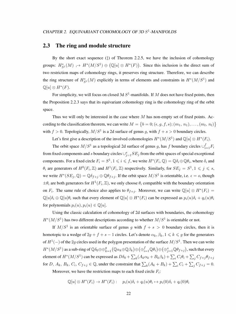
The orbit space M/S1 as a topological 2d surface of genus g, has f boundary circles ∪fi=1Fi
from fixed components and s boundary circles∪sj=1SEj from the orbit spaces of special exceptional
components. For a fixed circle Fi = S1, 1 6 i 6 f , we writeH∗(Fi,Q) = Qδi⊕Qθi, where δi and
θi are generators of H0(Fi,Z) and H1(Fi,Z) respectively. Similarly, for SEj = S1, 1 6 j 6 s,
we write H∗(SEj ,Q) = Qδf+j ⊕Qθf+j . If the orbit space M/S1 is orientable, i.e. ε = o, though
±θi are both generators for H1(Fi,Z), we only choose θi compatible with the boundary orientation
on Fi. The same rule of choice also applies to θf+j . Moreover, we can write Q[u] ⊗ H∗(Fi) =
Q[u]δi ⊕ Q[u]θi such that every element of Q[u] ⊗H∗(Fi) can be expressed as pi(u)δi + qi(u)θi
for polynomials pi(u), pi(u) ∈ Q[u].
Using the classic calculation of cohomology of 2d surfaces with boundaries, the cohomology
H∗(M/S1) has two different descriptions according to whether M/S1 is orientable or not.
If M/S1 is an orientable surface of genus g with f + s > 0 boundary circles, then it is
homotopic to a wedge of 2g + f + s− 1 circles. Let’s denote αk, βk, 1 6 k 6 g for the generators
ofH1(−) of the 2g circles used in the polygon presentation of the surfaceM/S1. Then we can write
H∗(M/S1) as a sub-ring of Qδ0⊕⊕gk=1
(Qαk⊕Qβk
)⊕(⊕fi=1Qθi
)⊕(⊕sj=1Qθf+j
), such that every
element of H∗(M/S1) can be expressed as Dδ0 +∑
k(Akαk +Bkβk) +∑
iCiθi +∑
j Cf+jθf+j
for D, Ak, Bk, Ci, Cf+j ∈ Q, under the constraint that∑
k(Ak +Bk) +∑
iCi +∑
j Cf+j = 0.
Moreover, we have the restriction maps to each fixed circle Fi:
Q[u]⊗H∗(Fi)→ H∗(Fi) : pi(u)δi + qi(u)θi 7→ pi(0)δi + qi(0)θi
22
CHAPTER 2. EQUIVARIANT COHOMOLOGY OF 3D S1-MANIFOLDS
and
H∗(M/S1)→ H∗(Fi) : Dδ0 +
g∑k=1
(Akαk +Bkβk) +
f∑i=1
Ciθi +s∑j=1
Cf+jθf+j 7→ Dδi +Ciθi
If M/S1 is a non-orientable surface of genus g with f + s > 0 boundary circles, then it is
homotopic to a wedge of g + f + s − 1 circles. We can denote αk, 1 6 k 6 g for the generators
of H1(−) of the g circles used in the polygon presentation of the surface M/S1. The description
of the cohomology H∗(M/S1) together with the restriction maps is similar to the orientable case,
with the only difference that there is no βk, Bk for the non-orientable case.
Following the above notations, we get
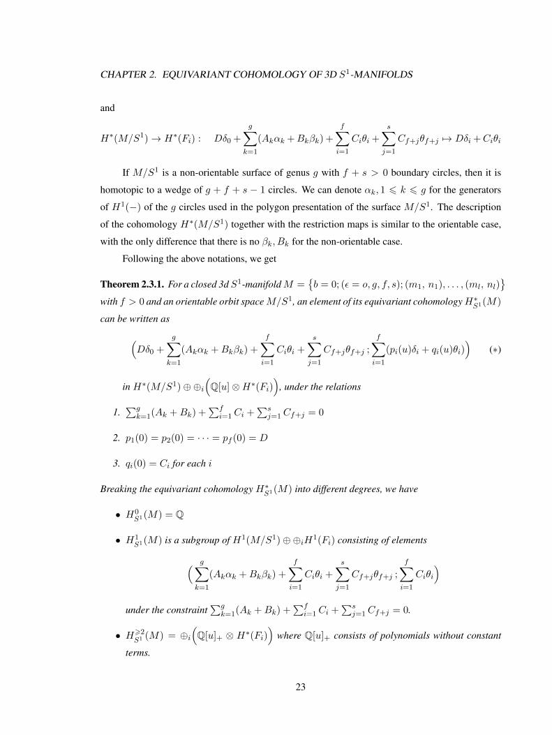
Theorem 2.3.1. For a closed 3d S1-manifoldM ={b = 0; (ε = o, g, f, s); (m1, n1), . . . , (ml, nl)
}with f > 0 and an orientable orbit spaceM/S1, an element of its equivariant cohomologyH∗S1(M)
can be written as
(Dδ0 +
g∑k=1
(Akαk +Bkβk) +
f∑i=1
Ciθi +
s∑j=1
Cf+jθf+j ;
f∑i=1
(pi(u)δi + qi(u)θi))
(∗)
in H∗(M/S1)⊕⊕i(Q[u]⊗H∗(Fi)
), under the relations
1.∑g
k=1(Ak +Bk) +∑f
i=1Ci +∑s
j=1Cf+j = 0
2. p1(0) = p2(0) = · · · = pf (0) = D
3. qi(0) = Ci for each i
Breaking the equivariant cohomology H∗S1(M) into different degrees, we have
• H0S1(M) = Q
• H1S1(M) is a subgroup of H1(M/S1)⊕⊕iH1(Fi) consisting of elements
( g∑k=1
(Akαk +Bkβk) +
f∑i=1
Ciθi +
s∑j=1
Cf+jθf+j ;
f∑i=1
Ciθi
)under the constraint
∑gk=1(Ak +Bk) +
∑fi=1Ci +
∑sj=1Cf+j = 0.
• H>2S1 (M) = ⊕i
(Q[u]+ ⊗ H∗(Fi)
)where Q[u]+ consists of polynomials without constant
terms.
23
CHAPTER 2. EQUIVARIANT COHOMOLOGY OF 3D S1-MANIFOLDS
Proof. The expression (∗) of elements of H∗S1(M) comes from the description of cohomologies
H∗(M/S1) and Q[u]⊗H∗(Fi). The relations (1)(2)(3) are due to the theorem 2.2.5 that H∗S1(M)
is the kernel of the restriction map H∗(M/S1) ⊕ ⊕i(Q[u] ⊗ H∗(Fi)
)→ ⊕iH∗(Fi). Thus, the
images of restrictions are the same: p1(0) = p2(0) = · · · = pf (0) = D, and qi(0) = Ci. Since
the relations (1)(2)(3) only live in degree less than 2, we get the description of H∗S1(M) in different
degrees.
Remark 2.3.2. For a closed 3d S1-manifoldM ={b = 0; (ε = n, g, f, s); (m1, n1), . . . , (ml, nl)
}with f > 0 and a non-orientable orbit space M/S1, the explicit expression of elements of H∗S1(M)
is almost the same as the oriented case, with the only modification that there is no βk, Bk term.
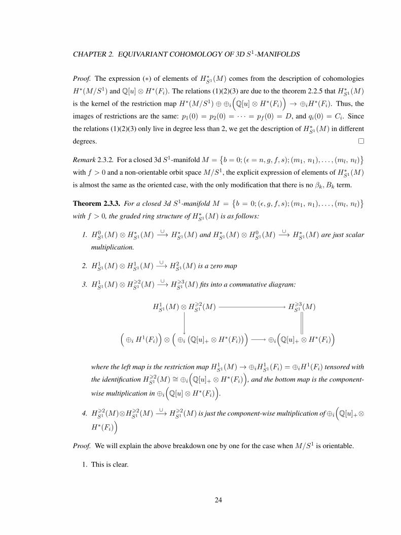
Theorem 2.3.3. For a closed 3d S1-manifold M ={b = 0; (ε, g, f, s); (m1, n1), . . . , (ml, nl)
}with f > 0, the graded ring structure of H∗S1(M) is as follows:
1. H0S1(M) ⊗ H∗S1(M)
∪−→ H∗S1(M) and H∗S1(M) ⊗ H0S1(M)
∪−→ H∗S1(M) are just scalar
multiplication.
2. H1S1(M)⊗H1
S1(M)∪−→ H2
S1(M) is a zero map
3. H1S1(M)⊗H>2
S1 (M)∪−→ H>3
S1 (M) fits into a commutative diagram:
H1S1(M)⊗H>2
S1 (M) H>3S1 (M)
(⊕i H1(Fi)
)⊗(⊕i(Q[u]+ ⊗H∗(Fi)
))⊕i(Q[u]+ ⊗H∗(Fi)
)
where the left map is the restriction map H1S1(M)→ ⊕iH1
S1(Fi) = ⊕iH1(Fi) tensored with
the identification H>2S1 (M) ∼= ⊕i
(Q[u]+ ⊗H∗(Fi)
), and the bottom map is the component-
wise multiplication in ⊕i(Q[u]⊗H∗(Fi)
).
4. H>2S1 (M)⊗H>2
S1 (M)∪−→ H>2
S1 (M) is just the component-wise multiplication of⊕i(Q[u]+⊗
H∗(Fi))
Proof. We will explain the above breakdown one by one for the case when M/S1 is orientable.
1. This is clear.
24
CHAPTER 2. EQUIVARIANT COHOMOLOGY OF 3D S1-MANIFOLDS
2. From the Theorem 2.3.1, H1S1(M) is generated by the basis αj , βj , θi, which have zero cup
product among them.
3. Similar to the above remark, the H1(M/S1) component of H1S1(M) ⊂ H1(M/S1) ⊕
⊕iH1(Fi) has zero cup-product. So only the cup product involving ⊕iH1(Fi) will survive.
4. Since H>2S1 (M) ∼= ⊕i
(Q[u]+⊗H∗(Fi)
), the cup product among H>2
S1 (M) is inherited from
⊕i(Q[u]+ ⊗H∗(Fi)
).
The argument is exactly the same for the case whenM/S1 is non-orientable, because of the Remark
2.3.2.
Using the cup product of Theorem 2.3.3, we can now describe the H∗S1(pt)-module structure
of H∗S1(M).
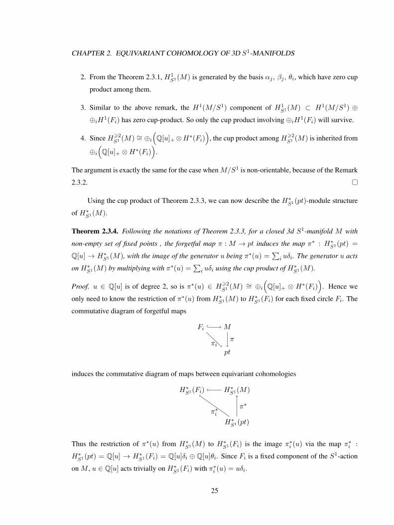
Theorem 2.3.4. Following the notations of Theorem 2.3.3, for a closed 3d S1-manifold M with
non-empty set of fixed points , the forgetful map π : M → pt induces the map π∗ : H∗S1(pt) =
Q[u] → H∗S1(M), with the image of the generator u being π∗(u) =∑
i uδi. The generator u acts
on H∗S1(M) by multiplying with π∗(u) =∑
i uδi using the cup product of H∗S1(M).
Proof. u ∈ Q[u] is of degree 2, so is π∗(u) ∈ H>2S1 (M) ∼= ⊕i
(Q[u]+ ⊗ H∗(Fi)
). Hence we
only need to know the restriction of π∗(u) from H∗S1(M) to H∗S1(Fi) for each fixed circle Fi. The
commutative diagram of forgetful maps
Fi M
ptπi
π
induces the commutative diagram of maps between equivariant cohomologies
H∗S1(Fi) H∗S1(M)
H∗S1(pt)
π∗iπ∗
Thus the restriction of π∗(u) from H∗S1(M) to H∗S1(Fi) is the image π∗i (u) via the map π∗i :
H∗S1(pt) = Q[u] → H∗S1(Fi) = Q[u]δi ⊕ Q[u]θi. Since Fi is a fixed component of the S1-action
on M , u ∈ Q[u] acts trivially on H∗S1(Fi) with π∗i (u) = uδi.
25

CHAPTER 2. EQUIVARIANT COHOMOLOGY OF 3D S1-MANIFOLDS
In conclusion, if we combine the contribution from all the fixed components Fi, we get
π∗(u) =∑
i uδi.
If a closed 3d S1-manifoldM does not have fixed point, then the image π∗(u) is inH2S1(M) ∼=
H2(M/S1) by the Proposition 2.2.3. In this case, a condition for π∗(u) = 0 is to make sure that
H2(M/S1) = 0.
Proposition 2.3.5. For a closed 3d fixed-point-free S1-manifoldM ={b; (ε, g, f = 0, s); (m1, n1), . . . , (ml, nl)
},
if ε = n or s > 0, then H2S1(M) ∼= H2(M/S1) = 0, hence π∗(u) = 0.
Proof. By the classic calculation of cohomology of surfaces. A sufficient condition forH2(M/S1) =
0 is that M/S1 is non-orientable or has non-empty boundary, which corresponds to the condition:
ε = n or s > 0.
If ε = o and s = 0, then this is exactly the case of oriented Seifert manifold. The image
π∗(u) ∈ H2S1(M) = H2(M/S1) is calculated by Niederkruger in his thesis (cf. [Ni05] Theorem
III.13).
Theorem 2.3.6 (Niederkruger, [Ni05]). Given an oriented Seifert manifoldM ={b; (ε = o, g, f =
0, s = 0); (m1, n1), . . . , (ml, nl)}
, let li be the unique solution of lini ≡ 1 mod mi, 0 < li < mi
for each coprime pair (mi, ni). Then
π∗(u) = b+
r∑i=1
limi∈ H2(M/S1) = Q
Remark 2.3.7. The rational number b+∑r
i=1 li/mi is exactly the orbifold Euler characteristic of the
oriented Seifert manifold, with integer b contributed by the principal orbits and fraction∑r
i=1 li/mi
contributed by the exceptional orbits.
2.4 The vector-space structure
Since we are working in Q-coefficient, the group structure of the equivariant cohomology
H∗S1(M) is simply the Q-vector-space structure. In the short exact sequence (‡), we note that the
surjective map Q[u] ⊗ H∗(F ) −→ H∗(F ) by sending a polynomial f(u) ∈ Q[u] to its constant
term f(0), has a kernel Q[u]+ ⊗ H∗(F ), where Q[u]+ consists of polynomials without constant
terms.
26

CHAPTER 2. EQUIVARIANT COHOMOLOGY OF 3D S1-MANIFOLDS
Proposition 2.4.1. Let M be a compact connected 3d effective S1-manifold(possibly with bound-
ary), and F be its fixed-point set(possibly empty), we get
H∗S1(M) ∼= H∗(M/S1)⊕(Q[u]+ ⊗H∗(F )
)as graded vector spaces
where Q[u]+ consists of polynomials without constant terms.
Proof. For a graded vector space, its isomorphism type is determined by the dimension at each
grading. In order to prove the proposition, we only need to show the dimension of H∗S1(M) is same
as the dimension of H∗(M/S1) ⊕(Q[u]+ ⊗ H∗(F )
)at each grading. From Theorem 2.2.5, we
knowH∗S1(M) is the kernel of the surjective mapH∗(M/S1)⊕(Q[u]⊗H∗(F )
)→ H∗(F ). Write
Q[u] = Q[u]+ ⊕ Q, then H∗(M/S1) ⊕(Q[u] ⊗H∗(F )
)= H∗(M/S1) ⊕
(Q[u]+ ⊗H∗(F )
)⊕(
Q⊗H∗(F ))
where the third summand Q⊗H∗(F ) is isomorphic to H∗(F ), and hence the direct
sum of the first two summands H∗(M/S1), Q[u]+ ⊗H∗(F ) is isomorphic to H∗S1(M) as graded
vector spaces.
Remark 2.4.2. The above expression of H∗S1(M) as a direct sum usually does not preserve the ring
structure, unless F = ∅, i.e. M is fixed-point-free.
Remark 2.4.3. If the fixed-point set MS1= F = ∪iFi is non-empty, then the orbit space M/S1
has boundaries, so H∗>2(M/S1) = 0. Also note Q[u]+ ⊗ H∗(Fi) has degrees at least 2. So the
above theorem says that when MS1 6= ∅, we have that H∗61S1 (M) ∼= H∗(M/S1) is determined by
the orbit space and H∗>2S1 (M) ∼= ⊕i
(Q[u]+ ⊗H∗(Fi)
)is determined by the fixed-point set.
2.5 Equivariant Betti numbers and Poincare series
Given an S1-manifold M , we can calculate its equivariant Betti numbers bkS1 = dimHkS1(M)
and the equivariant Poincare series PMS1 (x) =∑∞
k=0 bkS1x
k .
When a closed 3d S1-manifold M has neither fixed points nor special exceptional orbits, i.e.
f = s = 0, also called Seifert manifold, its orbit space M/S1 is a closed 2d orbifold of genus g.
By Proposition 2.2.3, H∗S1(M,Q) ∼= H∗(M/S1,Q) and the classic calculation of cohomology of
closed surfaces, we have
Proposition 2.5.1. For a closed 3d S1-manifold M without fixed points nor special exceptional
orbits, i.e. M ={b; (ε, g, f = 0, s = 0); (m1, n1), . . . , (ml, nl)
}, the equivariant Poincare series
are 1 + 2gx+ x2 if M is orientable, or 1 + gx if M is non-orientable.
27

CHAPTER 2. EQUIVARIANT COHOMOLOGY OF 3D S1-MANIFOLDS
When the set of fixed points or special exceptional orbits is non-empty, we will get:
Theorem 2.5.2. For a closed 3d S1-manifold M ={b; (ε, g, f, s); (m1, n1), . . . , (ml, nl)
}with
f + s > 0(hence b = 0), its equivariant Betti numbers are
b0S1 = 1
b1S1 =
2g + f + s− 1 if ε = o
g + f + s− 1 if ε = n
b2kS1 = f for k > 1
b2k+1S1 = f for k > 1
with the equivariant Poincare series
PMS1 (x) =∞∑k=0
bkS1xk =
1 + (2g + f + s− 1)x+ f · x2+x3
1−x2 if ε = o
1 + (g + f + s− 1)x+ f · x2+x3
1−x2 if ε = n
Proof. By Proposition 2.4.1, the equivariant cohomology of M is
H∗S1(M) ∼= H∗(M/S1)⊕⊕fi=1
(Q[u]+ ⊗H∗(Fi)
)as graded vector spaces
where Q[u]+ is the set of polynomials without constant terms and F = ∪fi Fi is the union of fixed
circles.
Note that, M/S1 is a 2d surface of genus g with f + s > 0 boundaries. Its Poincare series are
1 + (2g + f + s− 1)x if ε = o, or 1 + (g + f + s− 1)x if ε = n, using the classic result on the
cohomology of 2d surface with boundary. For each Q[u]+ ⊗ H∗(Fi), 1 6 i 6 f , it’s easy to see
that the Poincare series are x2
1−x2 · (1 + x).
Then we can calculate the equivariant Poincare series PMS1 (x) and equivariant Betti numbers
b∗S1 of M additively from those of M/S1 and Fi.
2.6 Equivariant formality
Using the explicit description of the ring and module structures, we can determine when a
closed 3d S1-manifold is equivariantly formal in the following sense.
Definition 2.6.1. A G-action on a manifold M is equivariantly formal, if the equivariant coho-
mology H∗G(M) is a free H∗G(pt)-module.
28
CHAPTER 2. EQUIVARIANT COHOMOLOGY OF 3D S1-MANIFOLDS
When talking about equivariant formality, we will only be interested in the case of closed
manifolds in this paper.
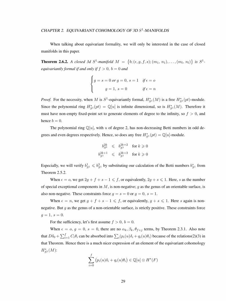
Theorem 2.6.2. A closed 3d S1-manifold M ={b; (ε, g, f, s); (m1, n1), . . . , (ml, nl)
}is S1-
equivariantly formal if and only if f > 0, b = 0 andg = s = 0 or g = 0, s = 1 if ε = o
g = 1, s = 0 if ε = n
Proof. For the necessity, when M is S1-equivariantly formal, H∗S1(M) is a free H∗S1(pt)-module.
Since the polynomial ring H∗S1(pt) = Q[u] is infinite dimensional, so is H∗S1(M). Therefore it
must have non-empty fixed-point set to generate elements of degree to the infinity, so f > 0, and
hence b = 0.
The polynomial ring Q[u], with u of degree 2, has non-decreasing Betti numbers in odd de-
grees and even degrees respectively. Hence, so does any free H∗S1(pt) = Q[u]-module.
b2kS1 6 b2k+2S1 for k > 0
b2k+1S1 6 b2k+3
S1 for k > 0
Especially, we will verify b1S1 6 b3S1 by substituting our calculation of the Betti numbers b∗S1 from
Theorem 2.5.2.
When ε = o, we get 2g + f + s− 1 6 f , or equivalently, 2g + s 6 1. Here, s as the number
of special exceptional components in M , is non-negative; g as the genus of an orientable surface, is
also non-negative. These constraints force g = s = 0 or g = 0, s = 1.
When ε = n, we get g + f + s − 1 6 f , or equivalently, g + s 6 1. Here s again is non-
negative. But g as the genus of a non-orientable surface, is strictly positive. These constraints force
g = 1, s = 0.
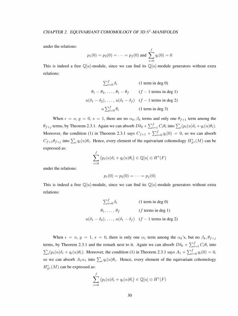
For the sufficiency, let’s first assume f > 0, b = 0.
When ε = o, g = 0, s = 0, there are no αk, βk, θf+j terms, by Theorem 2.3.1. Also note
that Dδ0 +∑f
i=1Ciθi can be absorbed into∑
i(pi(u)δi + qi(u)θi) because of the relations(2)(3) in
that Theorem. Hence there is a much nicer expression of an element of the equivariant cohomology
H∗S1(M):f∑i=0
(pi(u)δi + qi(u)θi
)∈ Q[u]⊗H∗(F )
29
CHAPTER 2. EQUIVARIANT COHOMOLOGY OF 3D S1-MANIFOLDS
under the relations:
p1(0) = p2(0) = · · · = pf (0) andf∑i=0
qi(0) = 0
This is indeed a free Q[u]-module, since we can find its Q[u]-module generators without extra
relations: ∑fi=0 δi (1 term in deg 0)
θ1 − θ2, . . . , θ1 − θf (f − 1 terms in deg 1)
u(δ1 − δ2), . . . , u(δ1 − δf ) (f − 1 terms in deg 2)
u∑f
i=0 θi (1 term in deg 3)
When ε = o, g = 0, s = 1, there are no αk, βk terms and only one θf+1 term among the
θf+j terms, by Theorem 2.3.1. Again we can absorb Dδ0 +∑f
i=1Ciθi into∑
i(pi(u)δi + qi(u)θi).
Moreover, the condition (1) in Theorem 2.3.1 says Cf+1 +∑f
i=0 qi(0) = 0, so we can absorb
Cf+1θf+j into∑
i qi(u)θi. Hence, every element of the equivariant cohomology H∗S1(M) can be
expressed as:f∑i=0
(pi(u)δi + qi(u)θi
)∈ Q[u]⊗H∗(F )
under the relations:
p1(0) = p2(0) = · · · = pf (0)
This is indeed a free Q[u]-module, since we can find its Q[u]-module generators without extra
relations: ∑fi=0 δi (1 term in deg 0)
θ1, . . . , θf (f terms in deg 1)
u(δ1 − δ2), . . . , u(δ1 − δf ) (f − 1 terms in deg 2)
When ε = n, g = 1, s = 0, there is only one α1 term among the αk’s, but no βk, θf+j
terms, by Theorem 2.3.1 and the remark next to it. Again we can absorb Dδ0 +∑f
i=1Ciθi into∑i(pi(u)δi + qi(u)θi). Moreover, the condition (1) in Theorem 2.3.1 says A1 +
∑fi=0 qi(0) = 0,
so we can absorb A1α1 into∑
i qi(u)θi. Hence, every element of the equivariant cohomology
H∗S1(M) can be expressed as:
f∑i=0
(pi(u)δi + qi(u)θi
)∈ Q[u]⊗H∗(F )
30
CHAPTER 2. EQUIVARIANT COHOMOLOGY OF 3D S1-MANIFOLDS
under the relations:
p1(0) = p2(0) = · · · = pf (0)
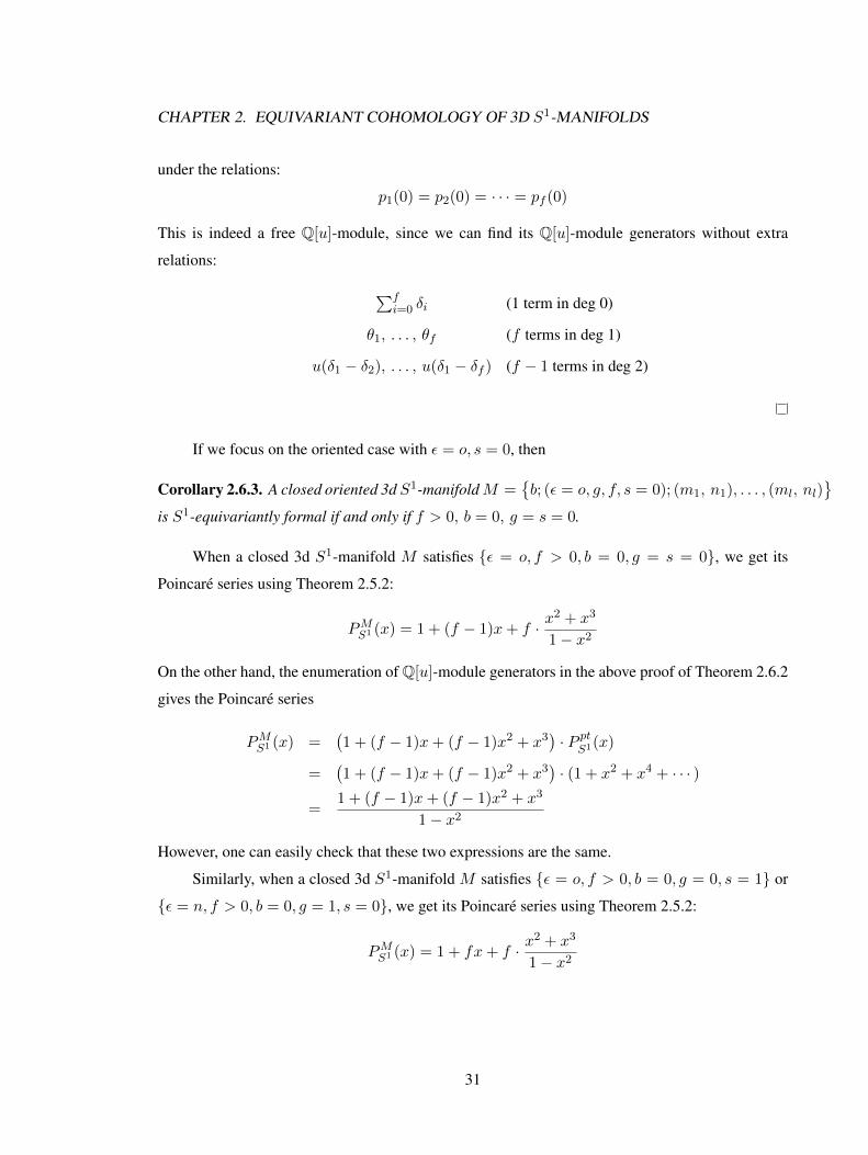
This is indeed a free Q[u]-module, since we can find its Q[u]-module generators without extra
relations:
∑fi=0 δi (1 term in deg 0)
θ1, . . . , θf (f terms in deg 1)
u(δ1 − δ2), . . . , u(δ1 − δf ) (f − 1 terms in deg 2)
If we focus on the oriented case with ε = o, s = 0, then
Corollary 2.6.3. A closed oriented 3d S1-manifoldM ={b; (ε = o, g, f, s = 0); (m1, n1), . . . , (ml, nl)
}is S1-equivariantly formal if and only if f > 0, b = 0, g = s = 0.
When a closed 3d S1-manifold M satisfies {ε = o, f > 0, b = 0, g = s = 0}, we get its
Poincare series using Theorem 2.5.2:
PMS1 (x) = 1 + (f − 1)x+ f · x2 + x3
1− x2
On the other hand, the enumeration of Q[u]-module generators in the above proof of Theorem 2.6.2
gives the Poincare series
PMS1 (x) =(1 + (f − 1)x+ (f − 1)x2 + x3
)· P pt
S1(x)
=(1 + (f − 1)x+ (f − 1)x2 + x3
)· (1 + x2 + x4 + · · · )
=1 + (f − 1)x+ (f − 1)x2 + x3
1− x2
However, one can easily check that these two expressions are the same.
Similarly, when a closed 3d S1-manifold M satisfies {ε = o, f > 0, b = 0, g = 0, s = 1} or
{ε = n, f > 0, b = 0, g = 1, s = 0}, we get its Poincare series using Theorem 2.5.2:
PMS1 (x) = 1 + fx+ f · x2 + x3
1− x2
31
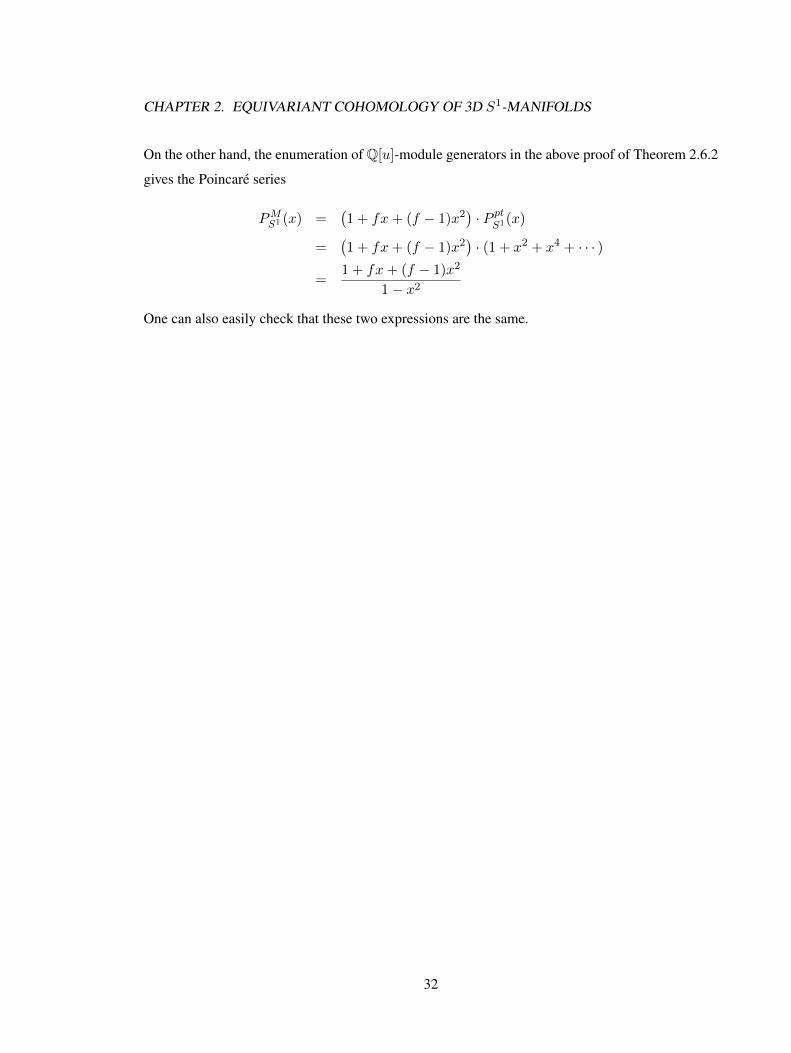
CHAPTER 2. EQUIVARIANT COHOMOLOGY OF 3D S1-MANIFOLDS
On the other hand, the enumeration of Q[u]-module generators in the above proof of Theorem 2.6.2
gives the Poincare series
PMS1 (x) =(1 + fx+ (f − 1)x2
)· P pt
S1(x)
=(1 + fx+ (f − 1)x2
)· (1 + x2 + x4 + · · · )
=1 + fx+ (f − 1)x2
1− x2
One can also easily check that these two expressions are the same.
32
Chapter 3
Localization of equivariant cohomology
of odd-dimensional manifold
With the even-dimensional GKM theory well established, it is natural to ask whether there
is a parallel odd-dimensional GKM theory. Goertsches, Nozawa and Toben [GNT12] developed a
GKM theory for a certain class of Cohen-Macaulay torus actions, including an application to certain
K-contact manifolds. In this paper, we will introduce similar results for odd-dimensional possibly
non-orientable manifolds.
3.1 Minimal 1-skeleton condition in odd dimension
As we have seen in the even-dimensional case, the essence of GKM theory is to find an ideal
condition for the application of Change-Skjelbred lemma 1.1.3. Here is the odd-dimensional version
of the GKM condition (or minimal 1-skeleton condition):
Definition 3.1.1 (GKM condition in odd dimension). An action of torus T on manifold (M2n+1, TM⊕Rk, J) is GKM if the fixed-point set MT is non-empty and the 1-skeleton M1 is at most of 3-
dimensional. Or equivalently,
(1) The fixed-point set MT consists of isolated circles.
(2) The 1-skeleton M1 is of dimension at most 3. Or equivalently, along each fixed circle γ ⊂MT , the non-zero weights [α1], . . . , [αn] ∈ t∗Z/±1 of the isotropy T -representation T y
TγM are pair-wise linearly independent.
33
CHAPTER 3. LOCALIZATION OF ODD-DIMENSIONAL MANIFOLD
From the condition (1), the fixed-point set MT consists of circles γ’s. We can fix a unit
orientation form θγ for each circle, and write
H∗T (MT ) = ⊕γ⊂MT
(H∗T (pt)⊗H∗(S1
γ))
= ⊕γ⊂MT
(St∗ ⊕ St∗θγ
)From the condition (2), similar to the even-dimensional case, along each fixed circle γ ⊂MT ,
we get pair-wise independent weights [α1], . . . , [αn] ∈ t∗Z/±1 of the isotropy T -representation. If
we denote Tαi to be the subtorus of T with Lie sub-algebra tαi = Kerαi, then the component C[αi]
of MTαi containing γ will be of dimension 3 with the residual action of the circle T/Tαi , i.e. a
non-trivial S1-action on 3-dimensional manifold with non-empty isolated fixed points.
3.2 The geometry and cohomology of 3d S1-manifolds
3-dimensional S1-manifolds without fixed points were classified by Seifert, hence are named
as Seifert manifolds. The case of 3-dimensional S1-manifolds with or without fixed points, also
called as generalized Seifert manifolds, were classified by Orlik and Raymond.
Briefly speaking, the equivariant diffeomorphism type of a 3-dimensional S1-manifold M3 is
determined by the orbifold type of its quotient space M/S1, the numeric data of the Seifert fibres
over orbifold points of M/S1, and the orbifold Euler number of the “fibration” M →M/S1.
Let’s denote ε and g as the orientability and genus of the orbifold surface M/S1, f as the
number of connected components in the fixed-point set MS1, s as the number of connected com-
ponents in MZ/2 whose normal spaces have the isotropy actions Z2reflecty R, and (µi, νi) as pairs
of Seifert invariants for connected components in MZ/µi whose normal spaces have the isotropy
actions Zµirotatey R2.
Theorem 3.2.1 (Orlik-Raymond classification of closed S1-manifolds, [Ra68, OR68]). Let S1 act
effectively and smoothly on a closed, connected smooth 3d manifold M . Then the orbit invariants{b; (ε, g, f, s); (m1, n1), . . . , (mr, nr)
}determine M up to equivariant diffeomorphisms, subject to certain conditions. Conversely, any
such set of invariants can be realized as a closed 3d manifold with an effective S1-action.
The proof of this theorem is by equivariant cutting and pasting, and furthermore inspires one
to compute its equivariant cohomology using Mayer-Vietoris sequences and classify equivariantly
formal S1-actions on 3d manifolds.
34
CHAPTER 3. LOCALIZATION OF ODD-DIMENSIONAL MANIFOLD
Theorem 3.2.2 (Equivariant formal 3d S1-manifold, [He] Theorem 4.8). A closed 3d S1-manifold
M ={b; (ε, g, f, s); (m1, n1), . . . , (mr, nr)
}is S1-equivariantly formal if and only if f > 0, b =
0 and one of the following three constraints holdsε = o, g = 0, s = 0
ε = o, g = 0, s = 1
ε = n, g = 1, s = 0
Moreover, in the orientable case of ε = o, g = 0, s = 0, the equivariant cohomologyH∗S1(M)
has the expression:f∑i=1
(Pi(u) +Qi(u)θi
)∈ ⊕i
(Q[u]⊗H∗(γi)
)where Pi, Qi ∈ Q[u] are polynomials, under the relations:
P1(0) = P2(0) = · · · = Pf (0) andf∑i=1
Qi(0) = 0
In the both non-orientable cases of ε = o, g = 0, s = 1 and ε = n, g = 1, s = 0, the equivariant
cohomology H∗S1(M) has the expression:
f∑i=0
(Pi(u) +Qi(u)θi
)∈ ⊕i
(Q[u]⊗H∗(γi)
)where Pi, Qi ∈ Q[u] are polynomials, under the relations:
P1(0) = P2(0) = · · · = Pf (0)
Transferring to a T -action on M3 with subtorus Tα acting trivially and the residual circle
T/Tα-action equivariantly formal,
1. when M is orientable, the equivariant cohomology H∗T (M3[α]) can be given as:
f∑i=0
(Pi +Qiθi
)∈ ⊕i
(St∗ ⊗H∗(γi)
)where Pi, Qi ∈ St∗ are polynomials, under the relations:
P1 ≡ P2 ≡ · · · ≡ Pf andf∑i=1
Qi ≡ 0 mod α (†)
35

CHAPTER 3. LOCALIZATION OF ODD-DIMENSIONAL MANIFOLD
2. when M is non-orientable, the equivariant cohomology H∗T (M3[α]) can be given as:
f∑i=0
(Pi +Qiθi
)∈ ⊕i
(St∗ ⊗H∗(γi)
)where Pi, Qi ∈ St∗ are polynomials, under the relations:
P1 ≡ P2 ≡ · · · ≡ Pf mod α (‡)
3.3 GKM graph and GKM theorem in odd dimension
Similar to the original even-dimensional GKM theory, we will construct GKM graphs for
odd-dimensional GKM manifolds and give a graph-theoretic computation of their equivariant coho-
mology.
In the even-dimensional case, the unique 2d S1-manifold with fixed points is the sphere S2
with exactly 2 fixed points. Each of such sphere gives rise to an edge connecting the 2 fixed points
in GKM graphs. However, in odd dimension, as we have seen in the previous discussion on 3d S1-
manifold with fixed points, there could be any positive number of fixed components, in contrast to
the exactly 2 fixed points of S2. Due to this difference, we need to modify the original construction
of GKM graphs a bit.
Definition 3.3.1 (GKM graph in odd dimension). The GKM graph for a GKM action of torus T
on M2n+1 consists of
Vertices There will be two types of vertices.
◦ for each fixed circle γ ⊂MT .
� for each 3d connected component C3[α] in MTα of some subtorus Tα of codimension 1.
Edges & Weights An edge joins a (�, C) to a (◦, γ), if the 3d manifold C contains the fixed circle
γ and hence is a connected component of MTα for an isotropy weight α of γ. The edge is
then weighted with α. There are no edges directly joining ◦ to ◦, nor � to �.
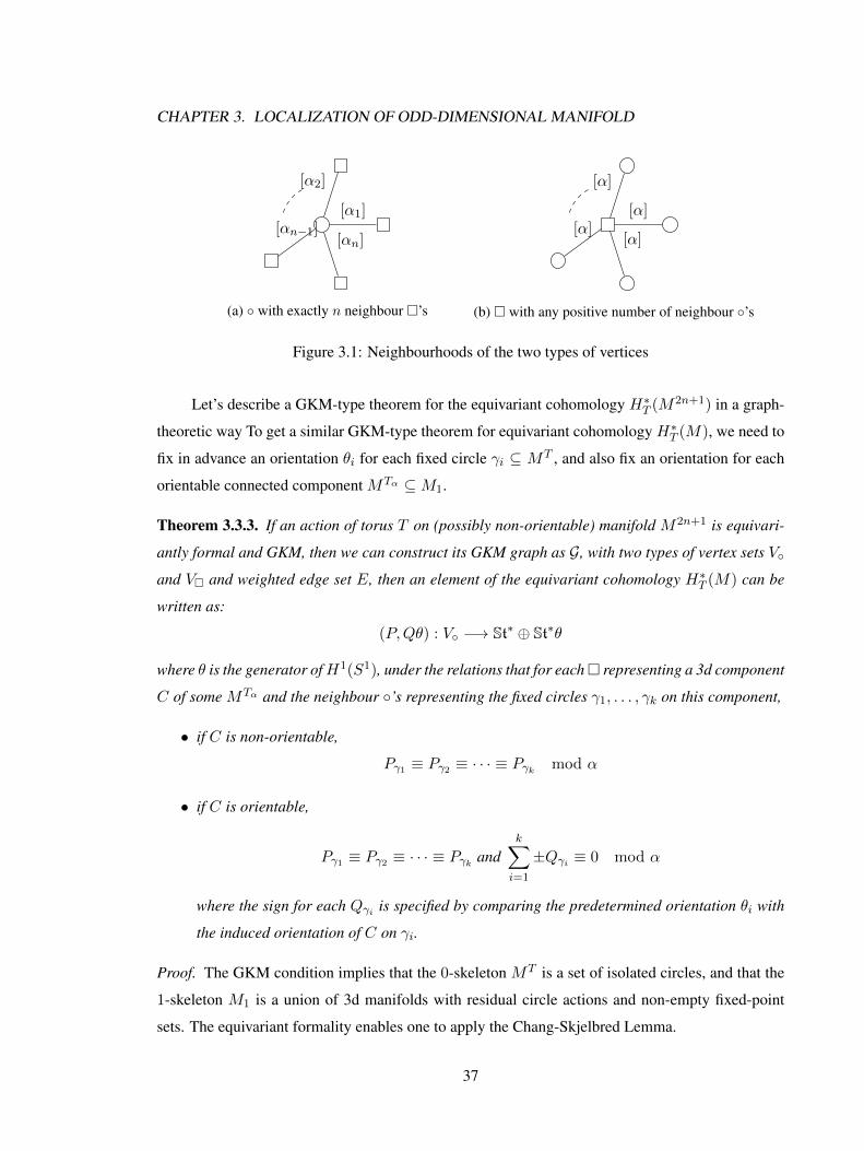
Remark 3.3.2. By the GKM condition 3.1.1, a fixed circle has exactly n pair-wise independent
weights. Thus each ◦, representing a fixed circle, is joined by exactly n edges to n �’s. Notice that
C as a connected component of MTα , can contain any positive number of fixed circles, and is also
a connected component of MT-α . Thus each �, representing a 3d component, can be joined by any
positive number of edges to ◦’s, with weight [α].
36
CHAPTER 3. LOCALIZATION OF ODD-DIMENSIONAL MANIFOLD
[α1]
[α2]
[αn−1][αn]
(a) ◦ with exactly n neighbour �’s
[α]
[α]
[α][α]
(b) � with any positive number of neighbour ◦’s
Figure 3.1: Neighbourhoods of the two types of vertices
Let’s describe a GKM-type theorem for the equivariant cohomology H∗T (M2n+1) in a graph-
theoretic way To get a similar GKM-type theorem for equivariant cohomology H∗T (M), we need to
fix in advance an orientation θi for each fixed circle γi ⊆ MT , and also fix an orientation for each
orientable connected component MTα ⊆M1.
Theorem 3.3.3. If an action of torus T on (possibly non-orientable) manifold M2n+1 is equivari-
antly formal and GKM, then we can construct its GKM graph as G, with two types of vertex sets V◦
and V� and weighted edge set E, then an element of the equivariant cohomology H∗T (M) can be
written as:
(P,Qθ) : V◦ −→ St∗ ⊕ St∗θ
where θ is the generator ofH1(S1), under the relations that for each� representing a 3d component
C of some MTα and the neighbour ◦’s representing the fixed circles γ1, . . . , γk on this component,
• if C is non-orientable,
Pγ1 ≡ Pγ2 ≡ · · · ≡ Pγk mod α
• if C is orientable,
Pγ1 ≡ Pγ2 ≡ · · · ≡ Pγk andk∑i=1
±Qγi ≡ 0 mod α
where the sign for each Qγi is specified by comparing the predetermined orientation θi with
the induced orientation of C on γi.
Proof. The GKM condition implies that the 0-skeleton MT is a set of isolated circles, and that the
1-skeleton M1 is a union of 3d manifolds with residual circle actions and non-empty fixed-point
sets. The equivariant formality enables one to apply the Chang-Skjelbred Lemma.
37
CHAPTER 3. LOCALIZATION OF ODD-DIMENSIONAL MANIFOLD
The equivariant cohomology H∗T (M) is embedded in H∗T (MT ) = ⊕γ⊂MT
(St∗ ⊗ H∗(γ)
).
In other words, to each fixed circle γ which is represented as a ◦ ∈ V◦, we associate a pair of
polynomials (Pγ , Qγθγ) ∈ St∗ ⊗H∗(γ).
By the Proposition 1.1.9 on inheritance of equivariant formality, every 3d T/Tα-componentC,
represented by a � ∈ V�, is also equivariantly formal. Then we can use the Classification Theorem
3.2.2 of equivariantly formal S1-actions on closed 3d manifolds, and the relations †, ‡ therein.
The only modifications are the signs in∑k
i=1±Qγi . Notice that in the Theorem 3.2.2, the
orientation forms θγ are chosen to be compatible with the orientation of the component C ⊂MTα ,
such that the isotropy weight of γ is exactly 1 under the residual S1 = T/Tα-action, or equivalently
with weight α under the T -action. However, if we have chosen orientations for the fixed circles
γ, then we need to adjust signs in the relation † for the difference of the chosen orientations and
compatible orientations. Because of the predetermination of orientations of γ, we can drop the
subscript and simply write θ universally as the orientation form for every γ.
Remark 3.3.4. If we reverse the predetermined orientation on a γi ⊆MT , then we just replace Qγiby−Qγi . If we reverse the predetermined orientation on an orientable componentC ofMTα ⊆M1,
then we just replace∑k
i=1±Qγi by∑k
i=1∓Qγi . Therefore, different choices of predetermined
orientations give isomorphic equivariant cohomology.
Remark 3.3.5. To describe the St∗-algebra structure, it is convenient to write an element (P,Qθ) as
(Pγ +Qγθ)γ⊂MT . Note θ2 = 0, then (Pγ +Qγθ)γ⊂MT +(Pγ + Qγθ)γ⊂MT = ([Pγ + Pγ ]+ [Qγ +
Qγ ]θ)γ⊂MT , and (Pγ +Qγθ)γ⊂MT · (Pγ + Qγθ)γ⊂MT = ([PγPγ ] + [PγQγ + PγQγ ]θ)γ⊂MT . For
any polynomial R ∈ St∗, we have R · (Pγ +Qγθ)γ⊂MT = (RPγ +RQγθ)γ⊂MT .
38

Chapter 4
Some applications
Next, we will give some examples of odd-dimensional GKM T -manifolds and apply the The-
orem 3.3.3 to describe equivariant cohomology with help of graphs.
4.1 Some direct examples
Example 4.1.1. All the 3d S1-equivariantly formal manifolds, that we used in Theorem 3.2.2,
are the building blocks of the odd-dimensional GKM theory. For any S1-equivariantly formal
orientable manifold M3 ={g = 0, ε = o, f > 0, s = 0, (µ1, ν1), . . . , (µr, νr)
}, the GKM
graph consists of one �-vertex, representing the manifold M , with f > 0 edges of weight 1 join-
ing to f ◦-vertices, representing the f fixed circles. The equivariant cohomology is H∗S1(M) ={(P1, Q1θ; . . . ;Pf , Qfθ) ∈ (Q[u] ⊕ Q[u]θ)⊕f | P1(0) = · · · = Pf (0),
∑fi=1Qi(0) = 0
}.
For any S1-equivariantly formal non-orientable manifold M3 ={g = 0, ε = o, f > 0, s =
1, (µ1, ν1), . . . , (µr, νr)}
or{g = 1, ε = n, f > 0, s = 0, (µ1, ν1), . . . , (µr, νr)
}, the GKM
graph is the same as the case of oriented case, but the equivariant cohomology is H∗S1(M) ={(P1, Q1θ; . . . ;Pf , Qfθ) ∈ (Q[u]⊕Q[u]θ)⊕f | P1(0) = · · · = Pf (0)
}.
Example 4.1.2. For the sphere S2n+1, we use the coordinates (z0, z1, . . . , zn) where zi’s are com-
plex variables. Let Tn act on S2n+1 by (eiθ1 , . . . , eiθn) · (z0, z1, . . . , zn) = (z0, eiθ1z1, . . . , e
iθnzn)
with fixed-point set (S2n+1)Tn
= {(z1, 0, . . . , 0) | |z1| = 1} ∼= S1. Since∑
dimH∗((S2n+1)Tn) =
2 =∑
dimH∗(S2n+1), the Tn action on S2n+1 is equivariantly formal by the formality criterion
Theorem 1.1.6. Let α1, . . . , αn be the standard integral basis of t∗Z = Zn, then the unique fixed cir-
cle has the unsigned isotropy weights [α1], . . . , [αn]. This means the action is GKM and the GKM
39
CHAPTER 4. SOME APPLICATIONS
graph consists of one ◦-vertex with n edges weighted [α1], . . . , [αn] joining to n �-vertices. The
equivariant cohomology is then H∗Tn(S2n+1) = {(P,Qθ) ∈ St∗ ⊕ St∗θ | Q ≡ 0 mod∏ni=1 αi}.
Example 4.1.3. The lens space Lm(1, l1, . . . , ln), where m > 1, l1, . . . , ln are positive integers
with the greatest common divisor 1, is defined as the quotient of a Z/mZ action on S2n+1: e2πi/m ·(z0, z1, . . . , zn) = (z0, e
2πl1i/mz1, . . . , e2πlni/mzn). Since the Tn action on S2n+1 in the previ-
ous example commutes with the Z/mZ action, the lens space Lm(1, l1, . . . , ln) inherits an in-
duced effective Tn action, as a quotient of S2n+1 by Z/mZ. The fixed-point set is a single
circle {(z1, 0, . . . , 0) | |z1| = 1} with isotropy weights [α1], . . . , [αn], hence the Tn action on
Lm(1, l1, . . . , ln) is GKM. Moreover, we still have the formality criterion∑
dimH∗(Lm(1, l1, . . . , ln)Tn) =
2 =∑
dimH∗(Lm(1, l1, . . . , ln)). The equivariant cohomology is againH∗Tn(Lm(1, l1, . . . , ln)) =
{(P,Qθ) ∈ St∗ ⊕ St∗θ | Q ≡ 0 mod∏ni=1 αi}.
Remark 4.1.4. We can equip S2n+1 with the standard contact form Θ = x0dy0− y0dx0 + x1dy1−y1dx1+· · ·+xndyn−yndxn where xj+iyj = zj and the induced contact form onLm(1, l1, . . . , ln).
Note the contact form is invariant under the Tn action used in previous two examples and one can
define moment maps for each generating vector field ∂∂θj
of the torus Tn as Θ( ∂∂θj
) = x2j + y2
j . The
hyperplane bundle (Ker Θ, ω = dΘ) is symplectic and hence is a complex vector bundle. This gives
Tn-invariant stable almost complex structure on S2n+1 and Lm(1, l1, . . . , ln), so that the weights
α1, . . . , αn are determined with signs.
Remark 4.1.5. Since we are using Q-coefficient and the ordinary cohomologyH∗(Lm(1, l1, . . . , ln),Q) ∼=H∗(S2n+1,Q), we get H∗Tn(Lm(1, l1, . . . , ln),Q) ∼= H∗Tn(S2n+1,Q) for equivariant cohomology,
though the formality criterion Theorem 1.1.6 only works for coefficients in Q,R,C not for Z.
Example 4.1.6. Take a product of an even-dimensional T k-equivariantly formal, GKM manifold
M2m and an odd-dimensional T l-equivariantly formal, GKM manifold N2n+1. The new 2(m +
n) + 1-dimensional manifold M × N under the product action of T k × T l is also equivariantly
formal and GKM. We can construct a GKM graph for M ×N out of the graphs of M and N . For
example, let’s try N = S1, and M an even-dimensional, stable almost complex manifold with a
T k-action. Then the GKM graph for T k action on M × S1 is obtained by replacing the •-vertices
of the graph of M into ◦-vertices and inserting a �-vertex at the center of each edge of the graph of
M . Since the weights of the standard S1-action on S2 at the two poles are 1 and −1, the weights of
the T -action on the S2[α] at the two poles N,S are α and −α, so are the weights of the T -action on
the S2[α] × S
1 at the two fixed circles {N} × S1, {S} × S1. This means that in the relation †, we
40
CHAPTER 4. SOME APPLICATIONS
get QN − QS ≡ 0 mod α, i.e. QN ≡ QS mod α. If we denote EM as the set of edges of the
GKM graph of M , then H∗T (M × S1) ={
(P,Qθ) : V → St∗ ⊕ St∗θ | Px ≡ Py and Qx ≡ Qy
mod α for each edge xy with weight [α] in EM}
= H∗T (M)⊗H∗(S1).
4.2 Odd-dimensional real and oriented Grassmannians
In this section, we compute equivariant cohomology rings of odd-dimensional real and ori-
ented Grassmannians, together with the canonical basis and characteristic basis of the additive
structure. We use the notation G2k+1(R2n+2), G2k+1(R2n+2) for the odd-dimensional real and
oriented Grassmannians of 2k + 1-dimensional subspaces in R2n+2.
4.2.1 Torus actions and 1-skeleton of odd-dimensional Grassmannians
First, we specify the torus actions on Grassmannians. Write the coordinates on R2n+2 as
(x1, y1, . . . , xn+1, yn+1). Let Tn act on R2n+2 so that the i-th S1-component of Tn exactly rotates
the i-th pairs of real coordinates (xi, yi) and leaves the remaining coordinates free, hence we can
write R2n+2 = (⊕ni=1R2[αi]
) ⊕ R20 for their decompositions into weighted subspaces, where [αi] ∈
t∗Z/± 1. These actions induce Tn actions on G2k+1(R2n+2), G2k+1(R2n+2).
Proposition 4.2.1 (1-skeleton of odd-dimensional real and oriented Grassmannians). The fixed
points, isotropy weights and 1-skeleta of G2k+1(R2n+2), G2k+1(R2n+2) can be given as
1. For G2k+1(R2n+2), there are(nk
)fixed circles of the form CS = {(⊕i∈SR2
[αi]) ⊕ L0 | L0 ∈
P(R20)} ∼= RP 1, where S is a k-element subset of {1, 2, . . . , n}. The isotropy weights at CS
are {[αj ±αi] | i ∈ S, j 6∈ S}∪ {[αi] | i ∈ S}∪ {[αj ] | j 6∈ S}, among which both [αj +αi]
and [αj −αi] join CS via a S2×RP 1 to C(S\{i})∪{j}, and [αi], [αj ] join CS via a RP 3 to no
other fixed circles.
2. For G2k+1(R2n+2), there are(nk
)fixed circles of the form CS = {(⊕i∈SR2
[αi]) ⊕ L0 | L0 ∈
G1(R20)} ∼= S1, where S is a k-element subset of {1, 2, . . . , n}. The isotropy weights at CS
are {[αj ±αi] | i ∈ S, j 6∈ S}∪ {[αi] | i ∈ S}∪ {[αj ] | j 6∈ S}, among which both [αj +αi]
and [αj − αi] join CS via a S2 × S1 to C(S\{i})∪{j}, and [αi], [αj ] join CS via a S3 to no
other fixed circles.
Proof. We give the details of the 1-skeleta of G2k+1(R2n+2). The case of G2k+1(R2n+2) is similar.
41
CHAPTER 4. SOME APPLICATIONS
Note that the Tn-fixed points of real Grassmannians are exactly the appropriate dimensional
sub-representations of the ambient representations and have the form (⊕i∈SR2[αi]
)⊕ L0 where S is
a k-element subset of {1, 2, . . . , n} and L0 ∈ P(R20). For each k-element subset S, the connected
component CS = {(⊕i∈SR2[αi]
)⊕ L0 | L0 ∈ P(R20)} ∼= RP 1 gives a fixed circle isolated from the
other fixed circles. This gives all the fixed points of the Tn action on G2k+1(R2n+2).
The tangent space at (⊕i∈SR2[αi]
) ⊕ L0 ∈ G2k+1(R2n+2), where L0 ∈ P(R20) has a L⊥0 ∈
P(R20) such that L0 ⊕ L⊥0 ∼= R2
0, is
HomR
((⊕i∈SR2
[αi])⊕ L0, (⊕j 6∈SR2
[αj ])⊕ L⊥0
)∼=(⊕i∈S ⊕j 6∈S
((R2
[αi])∗ ⊗R R2
[αj ]
))⊕(⊕i∈S (R2
[αi])∗ ⊗R L
⊥0
)⊕(⊕j 6∈S L∗0 ⊗R R2
[αj ]
)⊕(L∗0 ⊗R L
⊥0
)among which the first three terms and the fourth term give respectively the normal space and tangent
space of the fixed circle CS = {(⊕i∈SR2[αi]
)⊕ L0 | L0 ∈ P(R20)}.
It’s easy to see the weights of the tensor product (R2[αi]
)∗ ⊗R R2[αj ]
are [αj − αi], [αj + αi] ∈t∗Z/± 1. Let Tαj−αi and Tαj+αi be the subtori of Tn with Lie algebras annihilated by αj − αi and
αj + αi respectively. For the Tn-action on R2n = ⊕ni=1R2[αi]
, the fixed-point sets of Tαj−αi and
Tαj+αi onG2(R2[αi]⊕R2
[αj ]) are two 2-spheres sharing the poles which are exactly the two Tn-fixed
points R2[αi],R2
[αj ]∈ G2(R2
[αi]⊕ R2
[αj ]). We will denote the 2-spheres as S2
[αj−αi] and S2[αj+αi]
and
keep in mind that every element V in S2[αj−αi] or S2
[αj+αi]is a 2-plane in R2
[αi]⊕ R2
[αj ].
Now we are ready to describe the 1-skeleta: the Tn-fixed circle CS = {(⊕i′∈SR2[αi′ ]
) ⊕L0 | L0 ∈ P(R2
0)} ∼= RP 1 is joined to C(S\{i})∪{j} via {(⊕i′∈S\{i}R2[αi′ ]
) ⊕ V ⊕ L0 | V ∈S2
[αj−αi], L0 ∈ P(R20)} ∼= S2×RP 1 with weight [αj−αi] and also via {(⊕i′∈S\{i}R2
[αi′ ])⊕V ⊕L0 |
V ∈ S2[αj+αi]
, L0 ∈ P(R20)} ∼= S2 × RP 1 with weight [αj + αi]. Moreover, CS is contained
in {(⊕i′∈S\{i}R2[αi′ ]
) ⊕ W | W ∈ G3(R2[αi]⊕ R2
0)} ∼= RP 3 and {(⊕i′∈SR2[αi′ ]
) ⊕ L | L ∈P(R2
[αj ]⊕ R2
0)} ∼= RP 3 of weights [αi] and [αj ] respectively without other fixed points.
Using the description of 1-skeleton, we can give the graphs of 1-skeleton
Proposition 4.2.2. The odd-dimensional real and oriented GrassmanniansG2k+1(R2n+2), G2k+1(R2n+2)
have the same 1-skeleton graph consisting of
◦ vertices For each k-element subset S ⊆ {1, 2, . . . , n}, there is a ◦.
42

CHAPTER 4. SOME APPLICATIONS
� vertices, weights For each pair of different vertices S, S′ with S ∪ {j} = S′ ∪ {i}, there are
two �’s weighted [αj − αi] and [αj + αi] respectively. Near each S, there are n extra �’s
weighted [α1], . . . , [αn] respectively.
Edges For each ◦ with symbol S, we join it to all the nearby � vertices of its isotropy weights.
4.2.2 Equivariant cohomology of odd-dimensional real Grassmannian
In order to apply the Chang-Skjelbred lemma, we need to verify the equivariant formality. We
will first verify this for the odd-dimensional real Grassmannian G2k+1(R2n+2).
Theorem 4.2.3 (Poincare series of odd-dimensional real Grassmannians, [CK]). The Poincare se-
ries of G2k+1(R2n+2) are given as:
PG2k+1(R2n+2)(t) = (1 + t2n+1)PGk(Cn)(t2)
where the Poincare series of complex Grassmannian PGk(Cn) is (see Bott&Tu [BT82])
PGk(Cn)(t) =(1− t2) · · · (1− t2n)
(1− t2) · · · (1− t2k)(1− t2) · · · (1− t2(n−k))
Corollary 4.2.4. The total Betti number of G2k+1(R2n+2) is∑dimH∗(G2k+1(R2n+1)) = 2
(n
k
)Proposition 4.2.5 (Equivariant formality of torus actions on odd-dimensional real Grassmannians).
For the Tn-action on G2k+1(R2n+2), the isolated fixed circles CS are indexed on S = {S ⊆{1, 2, . . . , n} | #S = k}, and we have∑
dimH∗(G2k+1(R2n+1)Tn
) = #S ·∑
dimH∗(S1) = 2
(n
k
)Therefore, the torus actions on Gk(Rn) are equivariantly formal.
Proof. The verification is based on the criteria of equivariant formality Theorem 1.1.6, since the
total Betti number of G2k+1(R2n+2) is equal to that of the fixed-point set.
With the verifications of minimal 1-skeleton conditions and equivariant formality, we can give
the graphic description of the torus actions on Gk(Rn) by applying the Theorem 3.3.3.
43
CHAPTER 4. SOME APPLICATIONS
Theorem 4.2.6 (Equivariant cohomology of odd-dimensional real Grassmannian). Let S be the
collection of k-element subsets of {1, 2, . . . , n}. For odd dimensional GrassmannianG2k+1(R2n+2)
with Tn-action, an element of the equivariant cohomology is a set of polynomial pairs (fS , gSθ) to
each ◦-vertex S where θ is the unit volume form of S1 such that
1. gS ≡ 0 mod∏ni=1 αi for every S
2. fS ≡ fS′ , gS ≡ gS′ mod α2j − α2
i for S, S′ ∈ S with S ∪ {j} = S′ ∪ {i}
Corollary 4.2.7. There is an element rT ∈ H2n+1Tn (G2k+1(R2n+2)) such that (rT )2 = 0, and there
is a Q[α1, . . . , αn]-algebra isomorphism
H∗Tn(G2k+1(R2n+2)) ∼= H∗Tn(G2k(R2n))[rT ]/(rT )2
Proof. Comparing Example 1.2.14 with Theorem 4.2.6, we see the Tn-equivariant cohomologies
of G2k(R2n) and G2k+1(R2n+2) have the same congruence relations on the fS polynomials:
fS ≡ fS′ mod α2j − α2
i for S, S′ ∈ S with S ∪ {j} = S′ ∪ {i}
But the odd dimensional real Grassmannian has extra part of gSθ with congruence relations:
1. gS ≡ 0 mod∏ni=1 αi for every S
2. gS ≡ gS′ mod α2j − α2
i for S, S′ ∈ S with S ∪ {j} = S′ ∪ {i}
The first set of congruence relations means that
gS =( n∏i=1
αi)· hS
for a polynomial hS ∈ Q[α1, . . . , αn] and for every S. Substitute into the second set of congruence
relations, and note that∏ni=1 αi is coprime with α2
j − α2i , then we get
hS ≡ hS′ mod α2j − α2
i for S, S′ ∈ S with S ∪ {j} = S′ ∪ {i}
exactly the same as the congruence relations on the fS polynomials. Denote
rT =((
n∏i=1
αi)θ)S∈S
which has (rT )2 = 0 because θ is the unit volume form of S1, and has degree 2n+ 1 because each
αi is of degree 2 in cohomology. Then we can write
(fS + gSθ)S∈S = (fS)S∈S + rT · (hS)S∈S
44
CHAPTER 4. SOME APPLICATIONS
This establishes the bijection
H∗Tn(G2k+1(R2n+2)) ∼= H∗Tn(G2k(R2n))[rT ]/(rT )2
4.2.3 Equivariant cohomology of odd-dimensional oriented Grassmannian
There is a natural 2-covering of oriented Grassmannian over real Grassmannian π : Gk(Rn)→Gk(Rn) : v1∧· · ·∧vk 7→ SpanR(v1, . . . , vk) which induces a pull-back morphism π∗ : H∗(Gk(Rn))→H∗(Gk(Rn)) between their cohomologies. The non-trivial deck transformation is defined by re-
versing orientations ρ : Gk(Rn) → Gk(Rn) : v1 ∧ · · · ∧ vk 7→ −(v1 ∧ · · · ∧ vk) which induces an
isomorphism ρ∗ : H∗(Gk(Rn)) → H∗(Gk(Rn)). Both π and ρ commutes with the T -actions that
we introduced on the oriented Grassmannian and real Grassmannian.
For covering maps between compact spaces, or equivalently for free actions of finite groups,
there is a well-known fact relating their cohomologies in rational coefficients:
Lemma 4.2.8. Let π : X → Y be a covering between compact topological spaces with a finite deck
transformation group G which also acts on the cohomology H∗(X,Q). Then π∗ : H∗(Y,Q) →H∗(X,Q) is injective with image H∗(X,Q)G. This conclusion is also true for equivariant coho-
mology if a torus T acts on X and commutes with the action of G.
Proof. For a cocycle c of X , the averaged cocycle 1|G|∑
g∈G gc is invariant under G-action, hence
comes from a cocycle of Y . Consider the averaging map π∗ : H∗(X,Q) → H∗(Y,Q) : [c] 7→1|G| [∑
g∈G gc], then the composition π∗π∗ is the identity map on H∗(Y,Q), hence π∗ is injective.
Note that every cohomology class in H∗(X,Q)G can be represented by a G-invariant cocycle using
the averaging method. This proves the image of π∗ is exactly H∗(X,Q)G.
For the Tn-equivariant version, though the Borel construction X ×Tn (S∞)n, Y ×Tn (S∞)n
is not compact, we can apply the ordinary version of current Lemma to the compact approximations
X ×Tn (SN )n, Y ×Tn (SN )n for N →∞.
Remark 4.2.9. For the averaging method to work, we can relax the Q coefficients to be any coeffi-
cient ring that contains 1|G| . In R coefficients, the ordinary and equivariant de Rham theory together
with the averaging method gives a proof without using compact approximations.
Applying this Lemma to the oriented Grassmannian as a T -equivariant 2-cover over real Grass-
mannian, we get
45
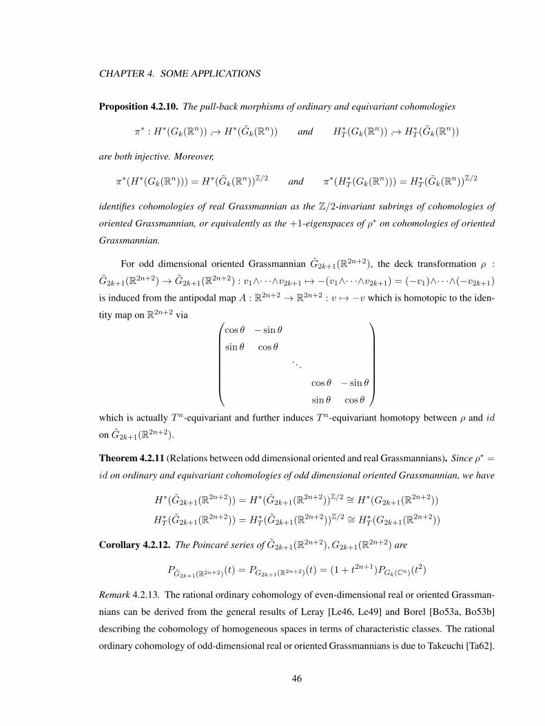
CHAPTER 4. SOME APPLICATIONS
Proposition 4.2.10. The pull-back morphisms of ordinary and equivariant cohomologies
π∗ : H∗(Gk(Rn)) ↪→ H∗(Gk(Rn)) and H∗T (Gk(Rn)) ↪→ H∗T (Gk(Rn))
are both injective. Moreover,
π∗(H∗(Gk(Rn))) = H∗(Gk(Rn))Z/2 and π∗(H∗T (Gk(Rn))) = H∗T (Gk(Rn))Z/2
identifies cohomologies of real Grassmannian as the Z/2-invariant subrings of cohomologies of
oriented Grassmannian, or equivalently as the +1-eigenspaces of ρ∗ on cohomologies of oriented
Grassmannian.
For odd dimensional oriented Grassmannian G2k+1(R2n+2), the deck transformation ρ :
G2k+1(R2n+2)→ G2k+1(R2n+2) : v1∧· · ·∧v2k+1 7→ −(v1∧· · ·∧v2k+1) = (−v1)∧· · ·∧(−v2k+1)
is induced from the antipodal map A : R2n+2 → R2n+2 : v 7→ −v which is homotopic to the iden-
tity map on R2n+2 via
cos θ − sin θ
sin θ cos θ
. . .
cos θ − sin θ
sin θ cos θ
which is actually Tn-equivariant and further induces Tn-equivariant homotopy between ρ and id
on G2k+1(R2n+2).
Theorem 4.2.11 (Relations between odd dimensional oriented and real Grassmannians). Since ρ∗ =
id on ordinary and equivariant cohomologies of odd dimensional oriented Grassmannian, we have
H∗(G2k+1(R2n+2)) = H∗(G2k+1(R2n+2))Z/2 ∼= H∗(G2k+1(R2n+2))
H∗T (G2k+1(R2n+2)) = H∗T (G2k+1(R2n+2))Z/2 ∼= H∗T (G2k+1(R2n+2))
Corollary 4.2.12. The Poincare series of G2k+1(R2n+2), G2k+1(R2n+2) are
PG2k+1(R2n+2)(t) = PG2k+1(R2n+2)(t) = (1 + t2n+1)PGk(Cn)(t2)
Remark 4.2.13. The rational ordinary cohomology of even-dimensional real or oriented Grassman-
nians can be derived from the general results of Leray [Le46, Le49] and Borel [Bo53a, Bo53b]
describing the cohomology of homogeneous spaces in terms of characteristic classes. The rational
ordinary cohomology of odd-dimensional real or oriented Grassmannians is due to Takeuchi [Ta62].
46
Bibliography
[A74] M. Atiyah, Elliptic operators and compact groups, Lecture Notes in Mathematics, vol. 401,
Springer-Verlag, Berlin-New York, 1974. ii+93 pp.
[AB84] M. Atiyah and R. Bott, The moment map and equivariant cohomology, Topology, 23:1-28,
1984.
[AP93] C. Allday and V. Puppe, Cohomological methods in transformation groups, Cambridge
Studies in Advanced Mathematics, vol. 32, Cambridge University Press, Cambridge, 1993.
[Au04] M. Audin, Torus actions on symplectic manifolds (Second revised edition), Progress in
Mathematics, vol. 93, Birkhauser Verlag, Basel, 2004.
[B72] G. Bredon, Introduction to compact transformation groups, Pure and Applied Mathematics,
vol. 46, Academic Press, New York-London, 1972.
[B74] G. Bredon, The free part of a torus action and related numerical equalities, Duke Math. J.
41 (1974), 843-854.
[Bo53a] A. Borel, Sur la cohomologie des espaces fibres principaux et des espaces homogenes de
groupes de Lie compacts. Ann. of Math. (2) 57, (1953). 115-207.
[Bo53b] A. Borel, La cohomologie mod 2 de certains espaces homognes, Comment. Math. Helv.
27, (1953). 165-197.
[Br97] M. Brion, Equivariant Chow groups for torus actions, Transform. Groups 2 (1997), no. 3,
225-267.
[BZ03] J. Bryden and P. Zvengrowski, The cohomology ring of the orientable Seifert manifolds II,
Topology Appl., 127:213–257, 2003.
47
BIBLIOGRAPHY
[BV83] N. Berline and M. Vergne, Zeros d’un champ de vecteurs et classes caracteristiques
equivariantes. Duke Math. J. 50 (1983), no. 2, 539-549.
[BT82] R. Bott and L. Tu, Differential forms in algebraic topology. Graduate Texts in Mathematics,
82. Springer-Verlag, New York-Berlin, 1982.
[CK] L. Casian and Y. Kodama, On the cohomology of real Grassmann manifolds, preprint,
https://arxiv.org/pdf/1309.5520v1.pdf
[CS74] T. Chang and T. Skjelbred, The topological Schur lemma and related results, Ann. of Math.,
100:307-321, 1974.
[Du94] J.J. Duistermaat, Equivariant cohomology and stationary phase, Contemp. Math., 179:45-
62, Amer. Math. Soc., Providence, RI, 1994.
[GGK02] V. Ginzburg, V. Guillemin and Y. Karshon, Moment maps, cobordisms, and Hamiltonian
group actions, Mathematical Surveys and Monographs, vol. 98, American Mathematical Society,
Providence, RI, 2002.
[GH04] V. Guillemin and T. Holm, GKM theory for torus actions with nonisolated fixed points,
Int. Math. Res. Not. 2004, no. 40, 2105-2124.
[GHZ06] V. Guillemin, T. Holm and C. Zara, A GKM description of the equivariant cohomology
ring of a homogeneous space, J. Algebraic Combin. 23 (2006), no. 1, 21-41.
[GKM98] M. Goresky, R. Kottwitz, R. MacPherson, Equivariant cohomology, Koszul duality, and
the localization theorem, Invent. Math., 131:25-83, 1998.
[GM14] O. Goertsches and A-L. Mare, Non-abelian GKM theory, Math. Z. 277 (2014), no. 1-2,
1-27.
[GNT12] O. Goertsches, H. Nozawa and D. Toben, Equivariant cohomology of K-contact mani-
folds, Math. Ann. 354 (2012), no. 4, 1555-1582.
[Go] R. Gonzales, Localization in equivariant cohomology and GKM theory, preprint,
http://www.ime.usp.br/˜jcarlson/palestra/GKM/loc_eq_cohom_
GKM(Gonzales,28pp).pdf.
[GS99] V. Guillemin and S. Sternberg, Supersymmetry and equivariant de Rham theory, Mathe-
matics Past and Present, Springer-Verlag, Berlin, 1999.
48
BIBLIOGRAPHY
[GSZ12] V. Guillemin, S. Sabatini and C. Zara, Cohomology of GKM fiber bundles, J. Algebraic
Combin. 35 (2012), no. 1, 19-59.
[GZ01] V. Guillemin and C. Zara, 1-skeleta, Betti numbers, and equivariant cohomology Duke
Math. J. 107 (2001), no. 2, 283-349.
[He] C. He, Classification and equivariant cohomology of circle actions on 3d manifolds, preprint,
http://arxiv.org/pdf/1608.02157v1.pdf
[Hs75] W.-Y. Hsiang, Cohomology theory of topological transformation groups, Ergebnisse der
Mathematik und ihrer Grenzgebiete, Band 85. Springer-Verlag, New York-Heidelberg, 1975.
x+164 pp.
[JN83] M. Jankins and W. Neumann, Lectures on Seifert manifolds, Vol. 2 of Brandeis Lecture
Notes, Brandeis University, Waltham, MA, 1983.
[KR03] A. Knutson and I. Rosu, Appendix to equivariant K-theory and equivariant cohomology,
Math. Z. 243 (2003), no. 3, 444-448.
[Le46] J. Leray, Sur l’anneau d’homologie de l’espace homogene, quotient d’un groupe clos par
un sousgroupe abelien, connexe, maximum. C. R. Acad. Sci. Paris 223, (1946). 412-415.
[Le49] J. Leray, Determination dans les cas non exceptionnels de l’anneau de cohomologie de
l’espace homogene quotient d’un groupe de Lie compact par un sous-groupe de meme rang. C.
R. Acad. Sci. Paris 228, (1949). 1902-1904.
[Ni05] K. Niederkruger, Compact Lie group actions on contact manifolds, PhD theis, University
of Cologne, 2005.
[Or72] P. Orlik, Seifert manifolds, Vol. 291 of Lecture Notes in Mathematics, Springer-Verlag,
Berlin-New York, 1972.
[OR68] P. Orlik and F. Raymond, Actions of SO(2) on 3-manifolds, Proc. Conf. on Transformation
Groups (New Orleans, La., 1967), 297-318, Springer, New York, 1968.
[Ra68] F. Raymond, Classification of the actions of the circle on 3-manifolds, Trans. Amer. Math.
Soc., 131:51-78, 1968.
[Sa56] I. Satake, On a generalization of the notion of manifold, Proc. Nat. Acad. Sci. U.S.A.,
42:359-363, 1956.
49
BIBLIOGRAPHY
[Se33] H. Seifert, Topologie Dreidimensionaler Gefaserter Raume, Acta Math., 1:147-238, 1933
[Ta62] M. Takeuchi, On Pontrjagin classes of compact symmetric spaces. J. Fac. Sci. Univ. Tokyo
Sect. I, 9 (1962) 313-328.
[VV03] G. Vezzosi and A. Vistoli, Higher algebraic K-theory for actions of diagonalizable groups
Invent. Math. 153 (2003), no. 1, 1-44.
50