arX

iv:1

309.

3680

v1 [

astr

o-ph

.HE

] 14

Sep

201

3

Astronomy & Astrophysicsmanuscript no. ms c© ESO 2013September 17, 2013

A new equilibrium torus solution and GRMHD initial conditio nsRobert F. Penna1, Akshay Kulkarni, and Ramesh Narayan2

1Department of Physics, and Kavli Institute for Astrophysics and Space Research, Massachusetts Institute of Technology, Cambridge,MA 02139, USA2Harvard-Smithsonian Center for Astrophysics, 60 Garden Street, Cambridge, MA 02138, USAe-mail:rpenna@mit.edu (RFP)

September 17, 2013

ABSTRACT

Context. General relativistic magnetohydrodynamic (GRMHD) simulations are providing influential models for black hole spin mea-surements, gamma ray bursts, and supermassive black hole feedback. Many of these simulations use the same initial condition: arotating torus of fluid in hydrostatic equilibrium. A persistent concern is that simulation results sometimes depend onarbitrary fea-tures of the initial torus. For example, the Bernoulli parameter (which is related to outflows), appears to be controlledby the Bernoulliparameter of the initial torus.Aims. In this paper, we give a new equilibrium torus solution and describe two applications for the future. First, it can be usedas amore physical initial condition for GRMHD simulations thanearlier torus solutions. Second, it can be used in conjunction with earliertorus solutions to isolate the simulation results that depend on initial conditions.Methods. We assume axisymmetry, an ideal gas equation of state, constant entropy, and ignore self-gravity. We fix an angular mo-mentum distribution and solve the relativistic Euler equations in the Kerr metric.Results. The Bernoulli parameter, rotation rate, and geometrical thickness of the torus can be adjusted independently. Our torus tendsto be more bound and have a larger radial extent than earlier torus solutions.Conclusions. While this paper was in preparation, several GRMHD simulations appeared based on our equilibrium torus. We believeit will continue to provide a more realistic starting point for future simulations.

1. Introduction

Accretion flows onto black holes are typically magnetizedand turbulent, so general relativistic magnetohydrodynamic(GRMHD) simulations have played an influential role inmodel building. The initial conditions for many of thesesimulations are the same: a rotating torus of fluid held to-gether by gravity, pressure gradients, and centrifugal forces(Fishbone & Moncrief, 1976; Fishbone, 1977; Kozlowski et al.,1978; Abramowicz et al., 1978; Chakrabarti, 1985). The en-tropy and angular momentum distribution of the torus are cho-sen arbitrarily and then hydrostatic equilibrium and an equa-tion of state fix the fluid’s density, velocity, and pressure.Atthe start of a simulation, the magnetorotational instability (MRI)(Balbus & Hawley, 1991, 1998) develops and the torus becomesturbulent. Turbulence transports angular momentum outward, al-lowing the fluid to accrete inwards, and the inner edge of thetorus becomes an accretion flow. The torus typically persiststhroughout the simulation and provides a reservoir of fluid feed-ing the outer edge of the accretion flow.

Simulations based on the equilibrium torus solutions ofFishbone & Moncrief (1976) and Chakrabarti (1985) havefound many applications: thin disk models (Shafee et al.,2008; Noble et al., 2009; Penna et al., 2010) black hole spinevolution (Gammie et al., 2004), radio emission from SgrA* (Noble et al., 2007; Dibi et al., 2012; Shcherbakov et al.,2012), black hole jets (McKinney, 2006, 2005; Nagataki,2009; Tchekhovskoy et al., 2011; Tchekhovskoy & McKinney,2012), computations of spectra (Hilburn et al., 2010), mag-netized accretion with neutrino losses (Barkov & Baushev,2011; Shibata et al., 2007; Barkov, 2008), pair production in

low luminosity galactic nuclei (Moscibrodzka et al., 2011),numerical convergence studies (Shiokawa et al., 2012), tilteddisk evolution (Fragile et al., 2007; Fragile & Blaes, 2008;Henisey et al., 2012), binary black hole mergers (Farris et al.,2011, 2012), and magnetically arrested disks (De Villiers et al.,2003; McKinney et al., 2012).

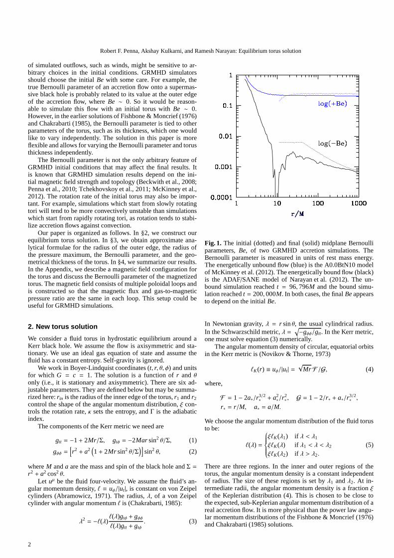
The equilibrium tori of Fishbone & Moncrief (1976) andChakrabarti (1985) are designed to be simple. They assume un-physical, power law angular momentum distributions in orderto keep the solutions analytical. When they are used as the ini-tial condition for GRMHD simulations, one hopes the turbulentaccretion flow “forgets” unrealistic features of the initial torus.However, this does not always seem to be the case. For exam-ple, the Bernoulli parameter of the initial torus appears topersistthrough to the final accretion flow (Figure 1).

The Bernoulli parameter is the sum of the kinetic energy,potential energy, and enthalpy of the gas (at least in Newtoniandynamics, where this splitting can be made precise. See§A.2 fora discussion of the GRMHD Bernoulli parameter.) At large dis-tances from the black hole, the potential energy vanishes. Sincethe other two terms are positive, gas at infinity must haveBe ≥ 0.Furthermore, in steady state and in the absence of viscosity, Be isconserved along streamlines. Hence any parcel of gas that flowsout with a positive value ofBe can potentially reach infinity. Aflow with positiveBe is called unbound and a flow with negativeBe is called bound. Unbound flows are more likely to generateoutflows.

As shown in Figure 1, the Bernoulli parameter of the accre-tion flows in some GRMHD simulations appears to be set bythe initial torus. This is a concern, as it suggests the strength

1

Robert F. Penna, Akshay Kulkarni, and Ramesh Narayan: Equilibrium torus solution

of simulated outflows, such as winds, might be sensitive to ar-bitrary choices in the initial conditions. GRMHD simulatorsshould choose the initialBe with some care. For example, thetrue Bernoulli parameter of an accretion flow onto a supermas-sive black hole is probably related to its value at the outer edgeof the accretion flow, whereBe ∼ 0. So it would be reason-able to simulate this flow with an initial torus withBe ∼ 0.However, in the earlier solutions of Fishbone & Moncrief (1976)and Chakrabarti (1985), the Bernoulli parameter is tied to otherparameters of the torus, such as its thickness, which one wouldlike to vary independently. The solution in this paper is moreflexible and allows for varying the Bernoulli parameter and torusthickness independently.

The Bernoulli parameter is not the only arbitrary feature ofGRMHD initial conditions that may affect the final results. Itis known that GRMHD simulation results depend on the ini-tial magnetic field strength and topology (Beckwith et al., 2008;Penna et al., 2010; Tchekhovskoy et al., 2011; McKinney et al.,2012). The rotation rate of the initial torus may also be impor-tant. For example, simulations which start from slowly rotatingtori will tend to be more convectively unstable than simulationswhich start from rapidly rotating tori, as rotation tends tostabi-lize accretion flows against convection.

Our paper is organized as follows. In§2, we construct ourequilibrium torus solution. In§3, we obtain approximate ana-lytical formulae for the radius of the outer edge, the radiusofthe pressure maximum, the Bernoulli parameter, and the geo-metrical thickness of the torus. In§4, we summarize our results.In the Appendix, we describe a magnetic field configuration forthe torus and discuss the Bernoulli parameter of the magnetizedtorus. The magnetic field consists of multiple poloidal loops andis constructed so that the magnetic flux and gas-to-magneticpressure ratio are the same in each loop. This setup could beuseful for GRMHD simulations.

2. New torus solution

We consider a fluid torus in hydrostatic equilibrium around aKerr black hole. We assume the flow is axisymmetric and sta-tionary. We use an ideal gas equation of state and assume thefluid has a constant entropy. Self-gravity is ignored.

We work in Boyer-Lindquist coordinates(t, r, θ, φ) and unitsfor which G = c = 1. The solution is a function ofr and θonly (i.e., it is stationary and axisymmetric). There are six ad-justable parameters. They are defined below but may be summa-rized here:rin is the radius of the inner edge of the torus,r1 andr2control the shape of the angular momentum distribution,ξ con-trols the rotation rate,κ sets the entropy, andΓ is the adiabaticindex.

The components of the Kerr metric we need are

gtt = −1+ 2Mr/Σ, gtφ = −2Mar sin2 θ/Σ, (1)

gφφ =[

r2 + a2(

1+ 2Mr sin2 θ/Σ)]

sin2 θ, (2)

whereM anda are the mass and spin of the black hole andΣ =r2 + a2 cos2 θ.

Let uµ be the fluid four-velocity. We assume the fluid’s an-gular momentum density,ℓ ≡ uφ/|ut|, is constant on von Zeipelcylinders (Abramowicz, 1971). The radius,λ, of a von Zeipelcylinder with angular momentumℓ is (Chakrabarti, 1985):

λ2 = −ℓ(λ)ℓ(λ)gtφ + gφφℓ(λ)gtt + gtφ

. (3)

Fig. 1. The initial (dotted) and final (solid) midplane Bernoulliparameters,Be, of two GRMHD accretion simulations. TheBernoulli parameter is measured in units of rest mass energy.The energetically unbound flow (blue) is the A0.0BtN10 modelof McKinney et al. (2012). The energetically bound flow (black)is the ADAF/SANE model of Narayan et al. (2012). The un-bound simulation reachedt = 96, 796M and the bound simu-lation reachedt = 200, 000M. In both cases, the finalBe appearsto depend on the initialBe.

In Newtonian gravity,λ = r sinθ, the usual cylindrical radius.In the Schwarzschild metric,λ =

√

−gφφ/gtt. In the Kerr metric,one must solve equation (3) numerically.

The angular momentum density of circular, equatorial orbitsin the Kerr metric is (Novikov & Thorne, 1973)

ℓK(r) ≡ uφ/|ut| =√

Mr F /G, (4)

where,

F = 1− 2a∗/r3/2∗ + a2

∗/r2∗ , G = 1− 2/r∗ + a∗/r

3/2∗ ,

r∗ = r/M, a∗ = a/M.

We choose the angular momentum distribution of the fluid torusto be:

ℓ(λ) =

ξℓK(λ1) if λ < λ1

ξℓK(λ) if λ1 < λ < λ2

ξℓK(λ2) if λ > λ2.

(5)

There are three regions. In the inner and outer regions of thetorus, the angular momentum density is a constant independentof radius. The size of these regions is set byλ1 andλ2. At in-termediate radii, the angular momentum density is a fraction ξof the Keplerian distribution (4). This is chosen to be closetothe expected, sub-Keplerian angular momentum distribution of areal accretion flow. It is more physical than the power law angu-lar momentum distributions of the Fishbone & Moncrief (1976)and Chakrabarti (1985) solutions.

2

Robert F. Penna, Akshay Kulkarni, and Ramesh Narayan: Equilibrium torus solution

The angular velocity of the torus is

Ω ≡ uφ

ut= −

gtφ + ℓgtt

gφφ + ℓgtφ. (6)

We have assumedur = uθ = 0, so this fully determines thevelocity.

Given the velocity of the torus, we can determine its densityand pressure from the Euler equation. Let

A ≡ ut =(

−gtt − 2Ωgtφ − Ω2gφφ)−1/2

, (7)

which sets the gravitational force felt by the fluid. The Eulerequation (Abramowicz et al., 1978) is then

∇pρ0 + U + p

= ∇ ln A − ℓ∇Ω1− Ωℓ . (8)

Our notation is standard:ρ0, U, and p are the mass density,internal energy, and gas pressure of the fluid in its rest frame.Euler’s equation describes the balance between pressure gradi-ents (LHS) and gravitational and centrifugal forces (RHS) re-quired for hydrostatic equilibrium.

To solve the Euler equation, it is helpful to introduce the ef-fective potential (Kozlowski et al., 1978)

W(r, θ) ≡ − ln(FA), (9)

where,

ln F(r, θ) ≡ −∫ rλm(r,θ)

rin

dΩdr

ℓdr1−Ωℓ . (10)

The lower limit of the integral,rin, is the radius of the inneredge of the torus. The upper limit,rλm(r, θ), is the equatorial ra-dius of the Von Zeipel cylinder containing (r, θ). For example,rλm(r, π/2) = r.

In terms of the effective potential, the Euler equation is

∇pρ0 + U + p

= −∇W. (11)

We can compute the effective potential because it depends onlyon ℓ. So the RHS is known. The boundary of the torus is theisopotential surfaceW(r, θ) = Win ≡ W(rin, π/2).

The specific enthalpy isw = 1+ ǫ + p/ρ0, whereǫ = U/ρ0is the specific internal energy.1 For an isentropic torus, the Eulerequation can be integrated to obtain (Kozlowski et al., 1978)

w(r, θ) = e−(W(r,θ)−Win). (12)

We assume the equation of statep = ρ0ǫ(Γ − 1), so the specificinternal energy is

ǫ = (w − 1)/Γ. (13)

The rest mass density and pressure are

ρ0 = [(Γ − 1)ǫ/κ]1/(Γ−1) , (14)

p = κρΓ0. (15)

The entropy,κ, is a free parameter. The torus is now fully deter-mined.

1 We caution thatǫ is used for two different but related conceptsin the literature. In older papers, such as Kozlowski et al. (1978), ǫis the total energy density,ρ0 + U. In more recent literature, such asDe Villiers et al. (2003),ǫ is the specific internal energy,U/ρ0. We fol-low the latter convention.

To summarize, we first choose the angular momentum distri-bution (5). The angular momentum distribution determines theangular velocity and effective potential. The effective potentialdetermines the enthalpy of the torus through Euler’s equation.Fixing an ideal gas equation of state and assuming an isentropictorus, gives the density, pressure, and internal energy. There aresix free parameters: the radius of the inner edge of the torus, rin,the break radii in the angular momentum distribution,r1 andr2,the normalization of the angular momentum,ξ, the entropy,κ,and the adiabatic index,Γ. The entropy simply sets the densityscale (equation 15) and, as there is no self-gravity, it has no effecton the dynamics.

3. Approximate analytical formulae

The solution of§2 can be implemented in GRMHD codes nu-merically. However, for physical understanding, it is useful tohave approximate formulae that describe the torus analytically.In this section, we obtain approximate analytical formulaeforthe outer edge, pressure maximum, geometrical thickness, andBernoulli parameter of the torus.

The most complicated feature of the exact solution is the in-tegral in equation (10). To obtain approximate analytical formu-lae for the torus, we need to simplify this integral. Let us firstrewrite it as

F = (1−Ωℓ) exp

(∫ rλm

rin

Ω

1−Ωℓdℓdr

dr

)

, (16)

where we have usedℓdΩ = d(Ωℓ) −Ωdℓ.In the inner region of the torus (λ < λ1), the angular mo-

mentum is constant and the integrand in equation (16) vanishes.So

F(r, θ) = 1−Ω(r, θ)ℓ(r, θ), (λ < λ1). (17)

In the outer region of the torus (λ > λ2), we may approximatethe integral by plugging the Newtonian formulaℓK(λ) =

√Mλ

into equation (5), and using the Newtonian angular velocityΩ(λ) = ℓ(λ)/λ2. Now integrating fromλ1 to λ2, we obtain

F ≈ (1−Ωℓ) I, (λ > λ2), (18)

where,

I ≡(

1− ξ2/λ2

1− ξ2/λ1

)1/2

. (19)

Equation (18) is approximate because we ignored special rela-tivistic contributions toℓ andΩ. But these are small in the outerregions of the torus. We can use our analytical approximation ofF to obtain simple formulae describing the torus.

3.1. Radius of the outer edge

The boundary of the torus is the isopotential surfaceW(r, θ) =Win = W(rin, π/2). We can simplifyW at the outer edge by usinga Newtonian description there. The equation for the outer radius,rout, becomes

Win ≈ −M

rout+ξ2Mr2

2r2out

− ln I. (20)

The solution for the outer radius is

rout/M ≈1+

√

1− ξ2λ2

, (21)

3

Robert F. Penna, Akshay Kulkarni, and Ramesh Narayan: Equilibrium torus solution

where

≡ 2 ln

[

AI

(

1− ℓ2

λ2

)]

r=rin

. (22)

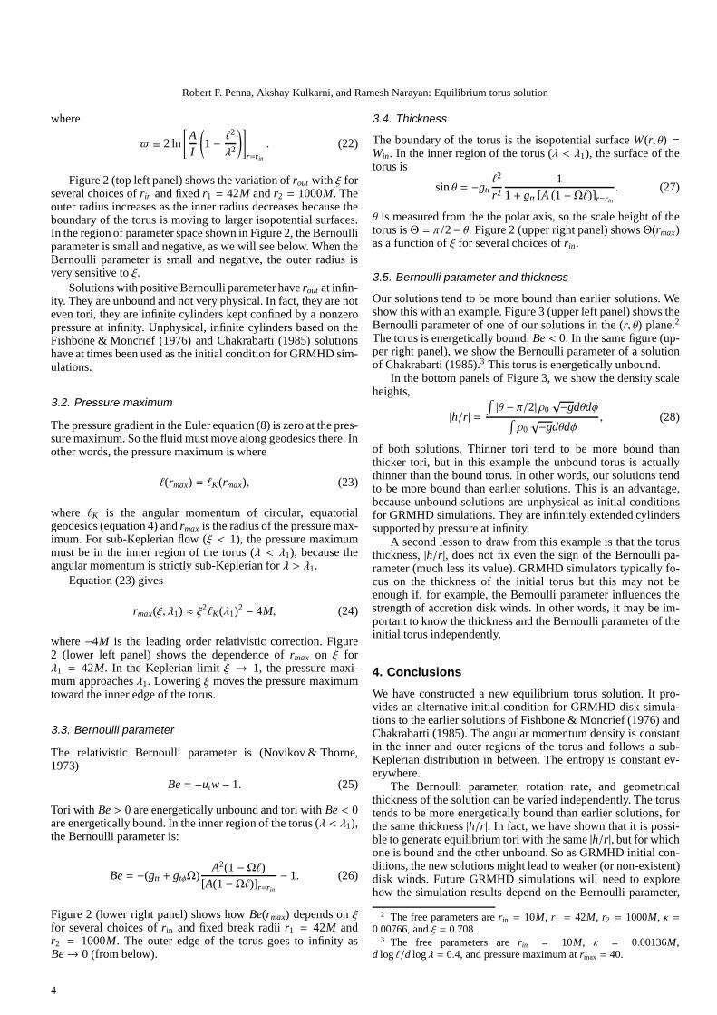
Figure 2 (top left panel) shows the variation ofrout with ξ forseveral choices ofrin and fixedr1 = 42M andr2 = 1000M. Theouter radius increases as the inner radius decreases because theboundary of the torus is moving to larger isopotential surfaces.In the region of parameter space shown in Figure 2, the Bernoulliparameter is small and negative, as we will see below. When theBernoulli parameter is small and negative, the outer radiusisvery sensitive toξ.

Solutions with positive Bernoulli parameter haverout at infin-ity. They are unbound and not very physical. In fact, they arenoteven tori, they are infinite cylinders kept confined by a nonzeropressure at infinity. Unphysical, infinite cylinders based on theFishbone & Moncrief (1976) and Chakrabarti (1985) solutionshave at times been used as the initial condition for GRMHD sim-ulations.

3.2. Pressure maximum

The pressure gradient in the Euler equation (8) is zero at thepres-sure maximum. So the fluid must move along geodesics there. Inother words, the pressure maximum is where

ℓ(rmax) = ℓK(rmax), (23)

where ℓK is the angular momentum of circular, equatorialgeodesics (equation 4) andrmax is the radius of the pressure max-imum. For sub-Keplerian flow (ξ < 1), the pressure maximummust be in the inner region of the torus (λ < λ1), because theangular momentum is strictly sub-Keplerian forλ > λ1.

Equation (23) gives

rmax(ξ, λ1) ≈ ξ2ℓK(λ1)2 − 4M, (24)

where−4M is the leading order relativistic correction. Figure2 (lower left panel) shows the dependence ofrmax on ξ forλ1 = 42M. In the Keplerian limitξ → 1, the pressure maxi-mum approachesλ1. Loweringξ moves the pressure maximumtoward the inner edge of the torus.

3.3. Bernoulli parameter

The relativistic Bernoulli parameter is (Novikov & Thorne,1973)

Be = −utw − 1. (25)

Tori with Be > 0 are energetically unbound and tori withBe < 0are energetically bound. In the inner region of the torus (λ < λ1),the Bernoulli parameter is:

Be = −(gtt + gtφΩ)A2(1−Ωℓ)

[A(1−Ωℓ)]r=rin

− 1. (26)

Figure 2 (lower right panel) shows howBe(rmax) depends onξfor several choices ofrin and fixed break radiir1 = 42M andr2 = 1000M. The outer edge of the torus goes to infinity asBe→ 0 (from below).

3.4. Thickness

The boundary of the torus is the isopotential surfaceW(r, θ) =Win. In the inner region of the torus (λ < λ1), the surface of thetorus is

sinθ = −gttℓ2

r2

11+ gtt [A (1−Ωℓ)]r=rin

. (27)

θ is measured from the the polar axis, so the scale height of thetorus isΘ = π/2− θ. Figure 2 (upper right panel) showsΘ(rmax)as a function ofξ for several choices ofrin.

3.5. Bernoulli parameter and thickness

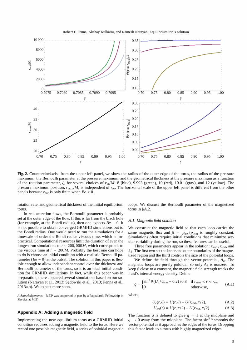
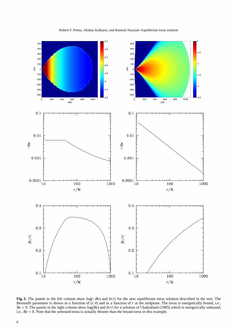
Our solutions tend to be more bound than earlier solutions. Weshow this with an example. Figure 3 (upper left panel) shows theBernoulli parameter of one of our solutions in the (r, θ) plane.2

The torus is energetically bound:Be < 0. In the same figure (up-per right panel), we show the Bernoulli parameter of a solutionof Chakrabarti (1985).3 This torus is energetically unbound.

In the bottom panels of Figure 3, we show the density scaleheights,

|h/r| =∫

|θ − π/2|ρ0√−gdθdφ

∫

ρ0√−gdθdφ

, (28)

of both solutions. Thinner tori tend to be more bound thanthicker tori, but in this example the unbound torus is actuallythinner than the bound torus. In other words, our solutions tendto be more bound than earlier solutions. This is an advantage,because unbound solutions are unphysical as initial conditionsfor GRMHD simulations. They are infinitely extended cylinderssupported by pressure at infinity.

A second lesson to draw from this example is that the torusthickness,|h/r|, does not fix even the sign of the Bernoulli pa-rameter (much less its value). GRMHD simulators typically fo-cus on the thickness of the initial torus but this may not beenough if, for example, the Bernoulli parameter influences thestrength of accretion disk winds. In other words, it may be im-portant to know the thickness and the Bernoulli parameter oftheinitial torus independently.

4. Conclusions

We have constructed a new equilibrium torus solution. It pro-vides an alternative initial condition for GRMHD disk simula-tions to the earlier solutions of Fishbone & Moncrief (1976)andChakrabarti (1985). The angular momentum density is constantin the inner and outer regions of the torus and follows a sub-Keplerian distribution in between. The entropy is constantev-erywhere.

The Bernoulli parameter, rotation rate, and geometricalthickness of the solution can be varied independently. The torustends to be more energetically bound than earlier solutions, forthe same thickness|h/r|. In fact, we have shown that it is possi-ble to generate equilibrium tori with the same|h/r|, but for whichone is bound and the other unbound. So as GRMHD initial con-ditions, the new solutions might lead to weaker (or non-existent)disk winds. Future GRMHD simulations will need to explorehow the simulation results depend on the Bernoulli parameter,

2 The free parameters arerin = 10M, r1 = 42M, r2 = 1000M, κ =0.00766, andξ = 0.708.

3 The free parameters arerin = 10M, κ = 0.00136M,d logℓ/d logλ = 0.4, and pressure maximum atrmax = 40.

4

Robert F. Penna, Akshay Kulkarni, and Ramesh Narayan: Equilibrium torus solution

0.7075 0.7080 0.7085 0.7090 0.70950

2000

4000

6000

8000

10 000

Ξ

r outM

0.70 0.75 0.80 0.85 0.90 0.95 1.000.10

0.15

0.20

0.25

0.30

0.35

Ξ

QHr=

r maxL

4

0.70 0.75 0.80 0.85 0.90 0.95 1.00

20

25

30

35

40

Ξ

r maxM

0.70 0.75 0.80 0.85 0.90 0.95 1.00

0.00

0.05

0.10

0.15

0.20

0.25

0.30

Ξ

BeHr=

r maxL

Fig. 2. Counterclockwise from the upper left panel, we show the radius of the outer edge of the torus, the radius of the pressuremaximum, the Bernoulli parameter at the pressure maximum, and the geometrical thickness at the pressure maximum as a functionof the rotation parameter,ξ, for several choices ofrin/M: 8 (blue), 9.993 (green), 10 (red), 10.01 (gray), and 12 (yellow). Thepressure maximum position,rmax/M, is independent ofrin. The horizontal scale of the upper left panel is different from the otherpanels becauserout is only finite whenBe < 0.

rotation rate, and geometrical thickness of the initial equilibriumtorus.

In real accretion flows, the Bernoulli parameter is probablyset at the outer edge of the flow. If this is far from the black hole(for example, at the Bondi radius), then one expectsBe ∼ 0. Itis not possible to obtain converged GRMHD simulations out tothe Bondi radius. One would need to run the simulations for atimescale of order the Bondi radius viscous time, which is im-practical. Computational resources limit the duration of even thelongest run simulations tot ∼ 200, 000M, which corresponds tothe viscous time atr ∼ 200M. Probably the best one can hopeto do is choose an initial condition with a realistic Bernoulli pa-rameter (Be ∼ 0) at the outset. The solution in this paper is flex-ible enough to allow independent control over the thicknessandBernoulli parameter of the torus, so it is an ideal initial condi-tion for GRMHD simulations. In fact, while this paper was inpreparation, there appeared several simulations based on our so-lution (Narayan et al., 2012; Sadowski et al., 2013; Penna et al.,2013a,b). We expect more soon.

Acknowledgements. R.F.P was supported in part by a Pappalardo Fellowship inPhysics at MIT.

Appendix A: Adding a magnetic field

Implementing the new equilibrium torus as a GRMHD initialcondition requires adding a magnetic field to the torus. Herewerecord one possible magnetic field, a series of poloidal magnetic

loops. We discuss the Bernoulli parameter of the magnetizedtorus in§A.2.

A.1. Magnetic field solution

We construct the magnetic field so that each loop carries thesame magnetic flux andβ = pgas/pmag is roughly constant.Simulations often require initial conditions that minimize sec-ular variability during the run, so these features can be useful.

Three free parameters appear in the solution:rstart, rend, andλB. The first two set the inner and outer boundaries of the magne-tized region and the third controls the size of the poloidal loops.

We define the field through the vector potential,Aµ. Themagnetic loops are purely poloidal, so onlyAφ is nonzero. Tokeepβ close to a constant, the magnetic field strength tracks thefluid’s internal energy density. Define

q =

sin3 θ (Uc/Ucm − 0.2) /0.8 if rstart< r < rend

0 otherwise,(A.1)

where,

Uc(r, θ) = U(r, θ) − U(rend, π/2), (A.2)

Ucm(r) = U(r, π/2)− U(rend, π/2). (A.3)

The functionq is defined to giveq = 1 at the midplane andq → 0 away from the midplane. The factor sin3 θ smooths thevector potential as it approaches the edges of the torus. Droppingthis factor leads to a torus with highly magnetized edges.

5

Robert F. Penna, Akshay Kulkarni, and Ramesh Narayan: Equilibrium torus solution

Fig. 3. The panels in the left column show log(−Be) and |h/r| for the new equilibrium torus solution described in the text. TheBernoulli parameter is shown as a function of (r, θ) and as a function ofr at the midplane. The torus is energetically bound, i.e.,Be < 0. The panels in the right column show log(Be) and|h/r| for a solution of Chakrabarti (1985) which is energeticallyunbound,i.e., Be > 0. Note that the unbound torus is actually thinner than the bound torus in this example.

6

Robert F. Penna, Akshay Kulkarni, and Ramesh Narayan: Equilibrium torus solution

Further define

f (r) = λ−1B

(

r2/3 + 15r−2/5/8)

. (A.4)

The vector potential is then

Aφ =

q sin( f (r) − f (rstart)) if q > 00 otherwise,

(A.5)

all otherAµ=0. (A.6)

The sinusoidal factor inAφ breaks the poloidal field into a seriesof loops. The functionf (r) gives each loop the same magneticflux. The number of loops is controlled byλB. The overall nor-malization ofAφ has not been specified so it can be tuned to giveany field strength.

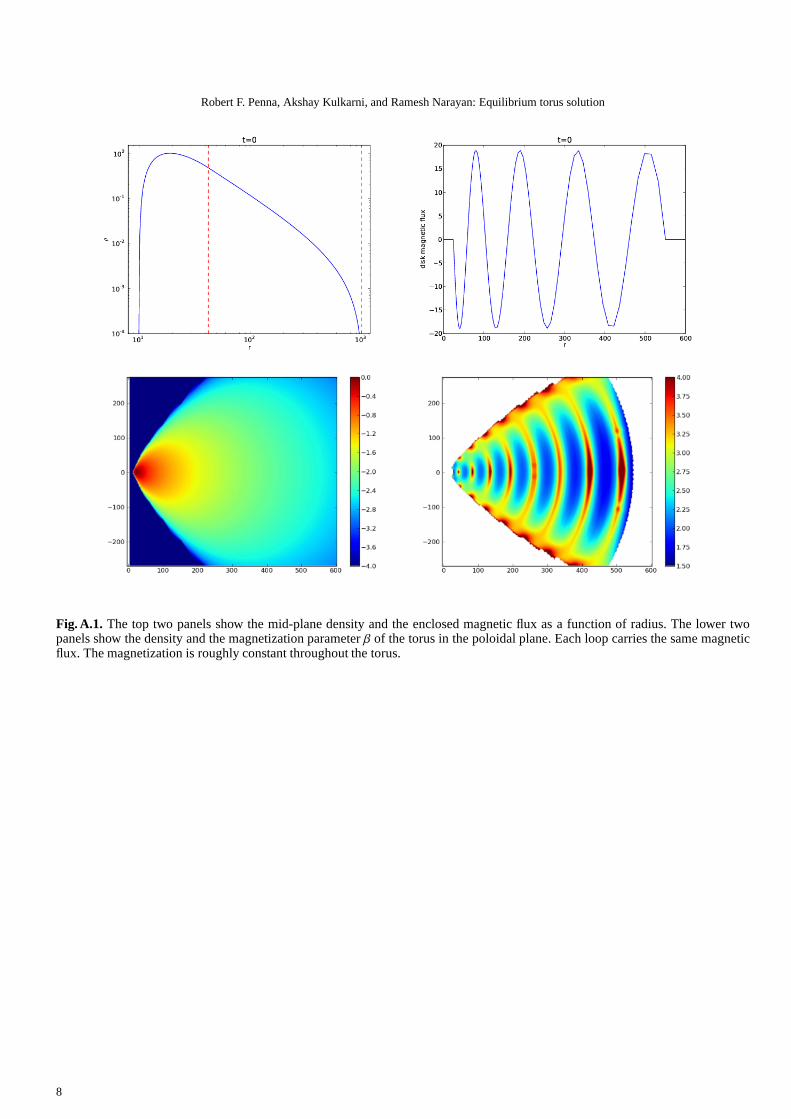
We give an example in Figure A.1. The equilibrium torus isas in Figure 3 and the field parameters arerstart= 25,rend= 550,andλB = 15/4. In this example there are eight magnetic loops.The magnetic flux,Aφ, peaks at the center of each loop, measuresthe flux carried by the loop, and is the same across the torus.The magnetizationβ = pgas/pmag peaks at loop edges and dropsat loop centers, but is roughly constant across the torus. Inthisexampleβ ∼ 100.

A.2. GRMHD Bernoulli parameter

The stress energy tensor of a magnetized fluid is

Tµν =

(

ρ0 + U +b2

2

)

uµuν +

(

pgas+b2

2

)

hµν − bµbν,

wherebµ is the magnetic field in the fluid’s rest frame andhµν =gµν+uµuν is the projection tensor. The magnetic field contributesb2/2 to the total internal energy andb2/2 to the total pressure,and introduces a stress term,−bµbν.

The Euler equations,h · (∇ · T ) = 0, become:

(

ρ0 + U + pgas+ b2)

a = −h · ∇(

pgas+b2

2

)

h − h · (b · ∇) b,

wherea = ∇uu is the fluid’s acceleration. We have used∇·b = 0to simplify the last term on the RHS.

Assume the flow is stationary and adiabatic, project the Eulerequations alongξ = ∂t, and combine terms using the first law ofthermodynamics. This leads to:

ddτ

(

ρ0 + U + pgas+ b2

ρ0ut

)

= − 1ρ0ξ · h · (b · ∇) b.

For the field configuration of§A.1, b is purely poloidal andξ · his purely toroidal. So the RHS is zero.

We thus obtain a straightforward generalization of equation(25):

Be = −(

1+U + pgas+ b2

ρ0

)

ut − 1. (A.7)

The unmagnetized torus hasBe ∼ −wgas. Adding magneticfields to the torus, with gas-to-magnetic pressure ratioβ =pgas/pmag, changes the Bernoulli parameter by terms of order1/β. Simulations typically have initialβ ∼ 100, in which casethe magnetic contribution to the Bernoulli parameter is of order1%.

ReferencesAbramowicz M., Jaroszynski M., Sikora M., 1978, A&A, 63, 221Abramowicz M. A., 1971, Acta Astron., 21, 81Balbus S. A., Hawley J. F., 1991, ApJ, 376, 214Balbus S. A., Hawley J. F., 1998, Reviews of Modern Physics, 70, 1Barkov M. V., 2008, in American Institute of Physics Conference Series, edited

by M. Axelsson, vol. 1054 of American Institute of Physics ConferenceSeries, 79–85

Barkov M. V., Baushev A. N., 2011, New A, 16, 46Beckwith K., Hawley J. F., Krolik J. H., 2008, ApJ, 678, 1180Chakrabarti S. K., 1985, ApJ, 288, 1De Villiers J., Hawley J. F., Krolik J. H., 2003, ApJ, 599, 1238Dibi S., Drappeau S., Fragile P. C., Markoff S., Dexter J., 2012, MNRAS, 426,

1928Farris B. D., Gold R., Paschalidis V., Etienne Z. B., ShapiroS. L., 2012, Physical

Review Letters, 109, 22, 221102Farris B. D., Liu Y. T., Shapiro S. L., 2011, Phys. Rev. D, 84, 2, 024024Fishbone L. G., 1977, ApJ, 215, 323Fishbone L. G., Moncrief V., 1976, ApJ, 207, 962Fragile P. C., Blaes O. M., 2008, ApJ, 687, 757Fragile P. C., Blaes O. M., Anninos P., Salmonson J. D., 2007,ApJ, 668, 417Gammie C. F., Shapiro S. L., McKinney J. C., 2004, ApJ, 602, 312Henisey K. B., Blaes O. M., Fragile P. C., 2012, ApJ, 761, 18Hilburn G., Liang E., Liu S., Li H., 2010, MNRAS, 401, 1620Kozlowski M., Jaroszynski M., Abramowicz M. A., 1978, A&A, 63, 209McKinney J. C., 2005, arXiv:astro-ph/0506369McKinney J. C., 2006, MNRAS, 368, 1561McKinney J. C., Tchekhovskoy A., Blandford R. D., 2012, MNRAS, 423, 3083Moscibrodzka M., Gammie C. F., Dolence J. C., Shiokawa H., 2011, ApJ, 735,

9Nagataki S., 2009, ApJ, 704, 937Narayan R., Sadowski A., Penna R. F., Kulkarni A. K., 2012, MNRAS, 426,

3241Noble S. C., Krolik J. H., Hawley J. F., 2009, ApJ, 692, 411Noble S. C., Leung P. K., Gammie C. F., Book L. G., 2007, Classical and

Quantum Gravity, 24, 259Novikov I. D., Thorne K. S., 1973, in Black Holes (Les Astres Occlus), edited

by C. Dewitt, B. S. Dewitt, 343–450Penna R. F., McKinney J. C., Narayan R., Tchekhovskoy A., Shafee R.,

McClintock J. E., 2010, MNRAS, 408, 752Penna R. F., Narayan R., Sadowski A., 2013a, MNRAS submitted,

arxiv:1307.4752Penna R. F., Sadowski A., Kulkarni A. K., Narayan R., 2013b,MNRAS, 428,

2255Sadowski A., Narayan R., Penna R. F., Zhu Y., 2013, MNRAS submitted,

arxiv:1307.1143Shafee R., McKinney J. C., Narayan R., Tchekhovskoy A., Gammie C. F.,

McClintock J. E., 2008, ApJ, 687, L25Shcherbakov R. V., Penna R. F., McKinney J. C., 2012, ApJ, 755, 133Shibata M., Sekiguchi Y. I., Takahashi R., 2007, Progress ofTheoretical Physics,

118, 257Shiokawa H., Dolence J. C., Gammie C. F., Noble S. C., 2012, ApJ, 744, 187Tchekhovskoy A., McKinney J. C., 2012, MNRAS, 423, L55Tchekhovskoy A., Narayan R., McKinney J. C., 2011, MNRAS, 418, L79

7

Robert F. Penna, Akshay Kulkarni, and Ramesh Narayan: Equilibrium torus solution

Fig. A.1. The top two panels show the mid-plane density and the enclosed magnetic flux as a function of radius. The lower twopanels show the density and the magnetization parameterβ of the torus in the poloidal plane. Each loop carries the samemagneticflux. The magnetization is roughly constant throughout the torus.

8