Localization in Sensor Network With Nystrom Approximation

8/3/2019 Localization in Sensor Network With Nystrom Approximation

http://slidepdf.com/reader/full/localization-in-sensor-network-with-nystrom-approximation 1/12

International Journal of Wireless & Mobile Networks (IJWMN) Vol. 3, No. 5, October 2011

DOI : 10.5121/ijwmn.2011.3504 37

LOCALIZATION IN SENSOR NETWORK WITH

N YSTROM A PPROXIMATION

Shailaja Patil1

and Mukesh Zaveri2

Department of Computer Engineering,

Sardar Vallabhbhai National Institute of Technology,

Surat, India,[email protected]; [email protected]

A BSTRACT

The recent innovations in wireless technology and digital electronics have opened many areas of

research in Wireless Sensor Networks. In the last few years these networks have been successfully used

in many applications such as localization, tracking, surveillance, battlefield monitoring, structural health

monitoring, routing etc. Most of these applications need localization i.e. estimating location informationeither relative or absolute. In this paper we propose a computationally efficient algorithm namely, Light

weight Multidimensional Scaling. This approach takes advantage of Nystr m approximation for

estimating location of unknown sensor nodes, using the information of available distances between

neighbours and anchors. Various node densities, noise factors and radio ranges are considered for

simulation. The performance of the algorithm is obtained with Monte Carlo Simulation.

K EYWORDS

Wireless sensor network, localization, Multidimensional scaling, Nystr m approximation

1. INTRODUCTION

Wireless Sensor Networks (WSNs) is a fast growing field which incorporates sensing,computation, and communication into a single tiny device. With the development of MEMS

technology, advancement in digital electronics, and wireless communications, it has been

possible to design small size, low cost energy efficient sensor nodes. These could be deployedin different environments and serve many applications such as military [1], environmental [2],

structure [3], safety and security [4] etc. WSNs are specifically important in the remote or

hazardous environment. Mostly, nodes are spread across the field in hundreds or in itsmultiples. The localization issue becomes important in case of uncertainty about some location

in critical applications. If the sensor network is used for monitoring an event in a building, the

exact location of each node can be known. However, if the sensor network is used formonitoring an event in a remote area like forest, nodes could be deployed from an airplane. In

such case, the precise location of most of the sensors is unknown. With the help of all theavailable information from the nodes, an effective localization algorithm can compute all the

positions. From last few years location based services have gained considerable attention fromthe researchers, and a lot of contribution have been made. Currently reported services and

applications consists of coverage analysis [5], location-aware applications [6], environmentalmonitoring [7], target tracking [8], intrusion detection [9], location based routing [10] etc. Adetailed survey of localization algorithms is provided in [11]. Localization algorithms enable

nodes to automatically determine their relative positions after deployment. The localization

algorithm should possess following characteristics:




38

• Energy efficiency (less computation, and communication)• Self-organization (independent of global infrastructure)

• Robust (being tolerant to range errors, and node failures),

We propose an algorithm based on Nystrm approximation of the eigenvectors of the large

matrix. It is a variant of Classical Multidimensional Scaling (CMDS) which not only preservesall of its attractive properties but also is computationally efficient. It is a two phase approach. In

the first phase, initial estimates are obtained with Nystrm approximation. These are furtherrefined using least square optimization in the second phase. Later, transformation is performed

to convert the local to global map. The paper is organized as follows. In Section II, we reviewthe literature of localization in WSNs. In Section III, we give the details of our proposedalgorithms. Section IV presents the simulation results and we conclude the paper in Section V.

2. RELATED WORK

The localization methods are broadly divided into range based methods that compute anestimation of the distances between two motes, or range-free methods, that depend on range

measurements. Range-based algorithms are based on hardware support by applying methodssuch as time of arrival (TOA) [12], time difference of arrival (TDOA) [12], angle of arrival

(AOA) [12], or radio signal strength indicator (RSSI) [13] technologies. On the contrary, rangefree algorithms are based on information of hop count or connectivity [14-15].

To obtain the location information, the Global Positioning System (GPS) [16] could be

used. However, there are limitations on use of GPS. It is not a cost effective solution for large-

scale ad-hoc networks in terms of price and energy. To assist in estimation of absolute

positions, a limited number of nodes whose position is known a-priory called anchors can beused. Anchors are supported by GPS or with manual configuration their location is obtained.

Most of the localization research has been carried out using anchor based approach [15-16, 22-

24].

The localization algorithm initially collects the distance information, and the number of

anchors, localization algorithm can be applied to estimate the location of the remaining nodes

of the network. There are several approaches developed by researchers in the literature of localization. For example Doherty et al. [18] provides a centralized method of the convex

optimization for position estimation and proposes a set of convex constraint models. Nodes

which are in the range of each other lie in a proximity constraint. To estimate globally optimumsolution, this convex constraint problem has been solved by semidefinite programming (SDP).

The localization problem has been formulated as linear programming model for directional

communication which is further solved by interior point method. This method needs to placeanchors at outer boundary preferably at the corners. If all anchors are placed at interior of thenetwork, the position estimation of outer nodes moves towards center showing large estimation

error. This technique has been extended by Biswas [19] with the non-convex inequalityconstraints. Basically, this technique converts the non-convex quadratic distance constraints

into linear constraints with introduction of relaxation to remove the quadratic term of the

equation. The distance measurements among nodes have been modeled as convex constraints,and to estimate the location of nodes semidefinite programming methods were adopted.Biswas's method was further improved by Tzu-Chen Liang [20], using a gradient search

technique. An approach with triangulation is presented in [21] called (APS) ‘Adhoc Positioning

System’. Three methods have been proposed by authors namely, DV-Hop, DV-Distance andEuclidean distance. DV - Hop method uses only connectivity information, whereas DV-

Distance uses the distance measurements between neighbouring nodes, and Euclidean uses the

local geometry of the nodes. Initially anchors flood their location to all the nodes in the network




39

and every unknown receiver node performs triangulation to three other anchor nodes toestimate the position. With anisotropic or irregular network topology, these methods do not

perform well. A two phase multilateration based algorithm called Hop-TERRAIN is proposed

in [22]. The first phase is similar to the DV-Hop [21], which does initial estimate of positions.In second phase, with the measured ranges and the location estimates of connected neighbours,

each sensor refines its estimation iteratively by triangulation. However, it only works for wellconnected nodes. In [23], authors have presented a triangulation based approach, where a

technique of iterative multiplication is used. It provides good results with more anchors. Nodesconnected to 3 or more anchors compute their position by triangulation and upgrade their

location. This position information is used by other unknown nodes for their position estimationin the next iteration. The algorithm of APS is refined using trilateration by adjustment called asLATN in [24]. In this method with DV-Hop or DV-Distance the positions are estimated and

trilateration is performed on unknown nodes for reducing the localization error. The leastsquares estimation with Kalman filter approach is used by Savvides [25] to locate the positions

of sensor nodes to reduce error accumulation in the same algorithm. This method also needsmore number of anchors to work well than other methods. Shang et al [14] presented a

centralized algorithm based on MDS, namely, MDS-MAP(C). Initially, using the connectivity

or distance information, a rough estimate of relative node distances is obtained. Then, MDS isused to obtain a relative map of the node positions and finally an absolute map is obtained withthe help of anchor nodes. The initial location estimation is refined using least square technique

in MDS-MAP (CR) [26]. Both techniques work well with few anchors and reasonably high

connectivity.

Shang et al. [27] proposed an improved version of MDS-MAP(C,R), called MDS-MAP (P),which eliminated the requirement of global connectivity information and centralized

computation. Here, an anisotropic sensor network is divided into a number of small regions,where each one is considered to be locally isotropic. Relative local maps are formed, and

merged into a global map. With this step, the characteristics of anisotropic were retained in theglobal map, and accuracy is improved. However, due to the error propagation during themerging process, its performance is affected.

In this paper, we present an energy efficient algorithm for localization of nodes usingNystrm approximation namely Light Weight MDS (LwMDS).

3. PROPOSED ALGORITHM

Multidimensional scaling methods are said to be computationally intensive since these use

singular value decomposition (SVD) of full distance matrix. With the proposed method, we

have shown that all unknown node locations can be estimated even with partial distance matrix.This can be achieved with Nystrm approximation. The anchor-anchor node distances andanchor to non-anchor node distances are required to estimate locations approximately. The

aforementioned approach also uses classical multidimensional scaling. However, there is asignificant difference between Nystrm approach and CMDS based approach. In CMDS based

methods, SVD is required to be applied on full distance matrix. This makes MDS

computationally intensive for real time use with large number of nodes, especially when theseare in thousands. With Nystrm approach, the SVD is applied on anchor to anchor distancematrix only, thus reducing its computational complexity. Due to this property, the algorithm is

named as Light Weight MDS (LwMDS). In this section a brief review of CMDS and its

relation with Nystrm approximation is presented. The proposed algorithm is described later.




40

3.1 Review of Classical MDS

MDS has its origin in psychometrics and psychophysics [30]. In the literature of localization,a number of techniques have been reported which use Multidimensional scaling. It is a set of

data analysis techniques which display distance like data as geometric structure. This method

is used for visualizing dissimilarity data. It is often used as a part of data exploratorytechnique or information visualization technique. MDS based algorithms are energy efficient

as communication among different nodes is required only initially for obtaining the inter-nodedistances of the network.

Multidimensional scaling algorithms map a distance matrix D between N items to a d

dimensional coordinate vector for each item. Entries in dissimilarity matrix are Euclidean

distances.Classical MDS consist of four steps:

1. Obtain the distance matrix D of Euclidean distances.

2. Apply double centering to this matrix. Double centering the distance matrix, converts it to anew matrix B as shown in equation (1)-

2 2 2 21/2( )ij ij i i ij i j ij i ij ij

B D e cD e c D cc D= − − − +∑ ∑ ∑ (1.1)

Where ei is the vector of ones.

The termi

i

c∑ =1, and its parameters determine the origin of the coordinate vectors. The

matrix B, also known as Gram or kernel matrix is a matrix of dot products between coordinate

vectors in that space [30].

3. Extract coordinate vectors from kernel matrix B using eigenvector decomposition.T

B Q Q= Λ (1.2)

Where Q is a matrix whose columns are orthonormal eigenvectors and Λ is a diagonal matrix of eigenvalues. The d dimensional coordinate vectors that form kernel matrix B can be seen as

scaled rows of Q. From the matrix Λ , highest d values are retained in order to minimize the

difference between original and embedded distances for d dimension. For d dimensionalextraction of coordinate vectors, we get two equations.

ij j i x Qλ = (i=1, 2…..N; j=1,2,… p)

(1.3)

Where λ 1 and λ 2 are first and second eigen values of the matrix Λ respectively.

3.2 Sensor Position Estimation by Nystrm Approximation and MDS

We use an approach from physics called Nystrm approximation [31]. This approximation

assumes that Gram matrix is positive semidefinite.Consider a network of N sensors with n beacons of known positions and ( N-n) of unknown

positions, present in a d dimension (2D or 3D). Let X and Y be the coordinate matrices of beacons and sensors of size n x d and ( N-n) x d respectively, and [X

TY

T]

Tbe the overall

coordinate matrix. The inner product between their coordinates is given by KM = [X Y] [XT

YT], which can be decomposed into four block sub-matrices [32], A = XX

T, Z = YX

T, C= YY

T

as below.

(1.4)

(1.5)

A Z

ZT

CKM=

E F

FT

GDM=

XXT

XTY

YTX YY

T

KM=




41

Where A and E have dimension n x n; Z and F have dimensions n x (N-n) and C and G havedimension ( N-n) x (N-n). As mentioned before matrix KM is a product of dot matrix, thus can

be expressed in terms of dot products of columns of matrices X and Y as in (1.5).As the matrix A=X

T X is a standard form of CMDS, the solution for X can be obtained by eigen

decomposing A:T

A UVU = (1.6)

Where U is a matrix whose columns are orthonormal eigenvectors and V is a diagonal matrix of eigenvalues. The coordinates can be obtained using (1.7)

T

d d X V U =

(1.7)

Where the subscript d is corresponding to dimension, first d largest positive eigen values. Thecoordinates of Z can be derived by solving the linear system as shown in (1.8)

ij j ij x v U = if i≤ n (1.8)

/ di dj j

d

Z U v= ∑ Otherwise

Where U ij is the ith component of j

theigenvector of A and v j is j

theigenvalue of A. Subscript J

varies from 1 to d , according to d dimensions.

(1 (1.9)

To find relation between Nystrm approximation, and MDS method, one has to consider sub-matrices E and F in place of A and Z. The centering coefficients in equation (1.1) can now be

changed as in (1.5).ci = 1/n if i≤ n

= 0 Otherwise (2.0)

Thus the centering formulas for A and Z in terms of E and F are :

2 2 2 2

2,

1 1 1 1( )

2ij ij i dj j iq ij

d q d q

A E e E e E E n n n

= − − − +∑ ∑ ∑ (2.1)

2 2 21 1 1( )

2ij ij i qj j id

d q

Z F e F e E n n

= − − −∑ ∑ (2.2)

Constant centring term is dropped from (2.2) as it causes irrelevant shift of origin. Thedimension, i varies from 1 to N, d varies from ( N-n) to N. Thus, as can be seen from equation

(1.8), advantage of Nystrm method is, coordinates of sensors can be computed using only the

information in A and Z matrices.Since these coordinates are determined in the space by the eigenvectors, it is necessary to

perform a final step of mapping them, with an affine transformation, into the initial space of anchors.

3.3 Light Weight MDS Algorithm (LwMDS)

Assume that nodes are randomly scattered in the region of consideration. Let pij refer to the

proximity measure between objects i and j. The simplest form of proximity can be representedusing Euclidean distance between two objects. This distance in m dimensional space is given by

(2.3)

A Z

ZT

ZT

A-1

Z

B=




42

2

1

( )m

ij ak bk

k

d X X =

= −∑ (2.3)

Where, X a (xa1 ; x a2 ;…. x am ) and X b ( xb1 ; x b2 ;…. x bm ) are distance vectors.

The steps of LwMDS are illustrated as below:

Phase 1:

Step 1:For a given region compute the shortest paths between every pair of nodes. These shortestpath distances are used to construct the distance matrix to be used for LwMDS. In this step

we assign distances to the edges of graph, if available. Remaining entries in distance

matrix are marked as infinity. The matrix completion is accomplished with Floyd’s

algorithm.2 2

12 1

2 2 2

21 23 2

2

2 2 2

1 2 3

0 .. ..

0 ..

.. .. 0 .. ..

.. .. .. 0 ..

.. 0

n

n

n n n

d d

d d d

D

d d d

= (2.4)

The time complexity of the aforementioned algorithm is O( N 3),where N is number of

nodes.

Step 2:Apply MDS to the anchor-anchor distance matrix. Retain first two or three largest eigen-

values and eigenvectors according to the requirement of dimensions (2D or 3D). Let A besuch distance vector. Applying SVD to A yields,

T A UVU = (2.5)

Obtain the local coordinates with T

d d X V U = with first d largest positive eigen values .

This step reduces complexity with large factor. As complexity of CMDS is dominated byeigenvalue problem, for a fully symmetric matrix [ NxN ] ,it costs O( N 3) for N number of

nodes,whereas for LwMDS it is O(n3)(n is number of anchors).

Step 3:Using Nystrm approximation to anchor node’s distance matrix, obtain the embedding of

( N-n) sensor nodes, and relative map of N nodes with equations expressed in (1.8).

Phase 2:

Step 4:Apply least square minimization to refine estimated positions.This step includes refinement of estimated positions to improve the absolute map. The least

square minimization algorithm is used to minimize the error between estimated and truepositions. The complexity of this method is O(n

3). Least square minimization problem has

lots of local minima and with random starting points a wrong solution may be obtained.

However, positions provided by CMDS have proved to be good starting points forminimization problems [26].

Step 5:

With the information of absolute positions of anchor nodes transform relative map toabsolute map. This step converts relative map to absolute map. This transformation

includes scaling, rotation, reflection etc. This step is necessary to minimize the sum of

squares of errors between actual positions of anchors and their relative positions in the




43

MDS map. For n number of anchor nodes, this transformation computation takes O(n3)

time. Applying this transformation to the whole relative map takes O( N ) time.

4. SIMULATION RESULTS

The density of nodes is varied from 50-200, and are considered to be placed randomly with auniform distribution in a square area with some ranging errors. In a square area of l unit length

n2 nodes are placed in nl by nl square. The radio range is R. The actual distance is blurred with

Gaussian noise. Uniform radio propagation is considered. The noise is added to radio range

from 5% to 20%. Number of anchors is varied from 4 to 10. The Monte Carlo simulation havebeen performed, and the number of simulations for each experiment is set to 30. We have

compared our results with MDS-MAP(C,R). Results of LwMDS for 200 nodes with isotropic

topology are presented here.

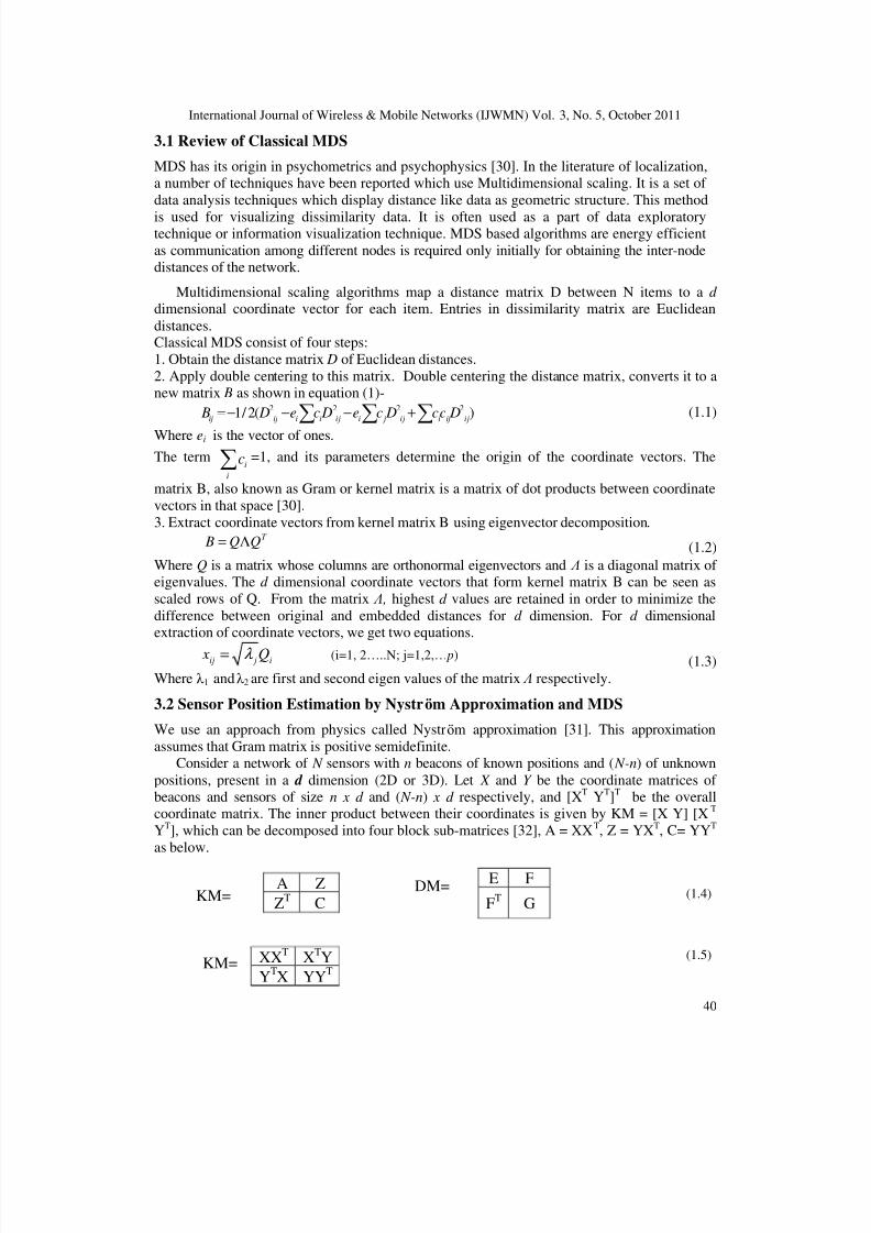
Figure 1: Isotropic network with average connectivity of 12

Fig.(1) shows a similar scenario for 200 nodes spread randomly in a square area of 10 units X

10 units. Stars (*) depict nodes and lines are the radio link between nodes forming theconnectivity of 12. Diamonds are anchors selected randomly. With various radio ranges the

connectivity level has been estimated with 200 nodes, and it is observed that the network becomes fully connected from the connectivity of greater than 12.

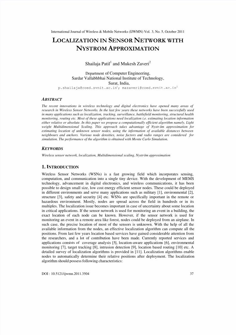
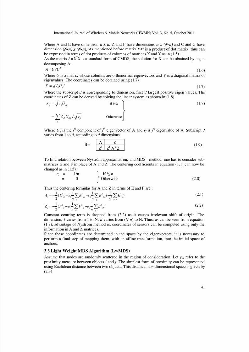
Fig.2: Participation of nodes in the network connectivity

The fraction of nodes participating in the network connectivity with increasing radio range is

shown in Fig (2). As can be seen, with the average connectivity of 10, for radio range of 1.3,

about 195 nodes take active part in forming the network. As the radio range is increased to 1.5all the nodes come into the network. The full connectivity of network for all possible scenarios

of simulation is obtained from connectivity of 20 onwards. We have estimated the embedding




44

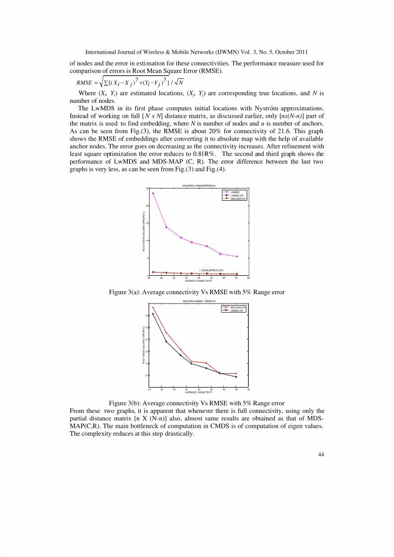
of nodes and the error in estimation for these connectivities. The performance measure used forcomparison of errors is Root Mean Square Error (RMSE).

2 2[( ) ( ) ] / RMSE X X Y Y N i j i j= − + −∑

Where ( X i , Y i) are estimated locations, ( X j , Y j) are corresponding true locations, and N is

number of nodes.The LwMDS in its first phase computes initial locations with Nystrm approximations.

Instead of working on full [ N x N ] distance matrix, as discussed earlier, only [nx(N-n)] part of the matrix is used to find embedding, where N is number of nodes and n is number of anchors.

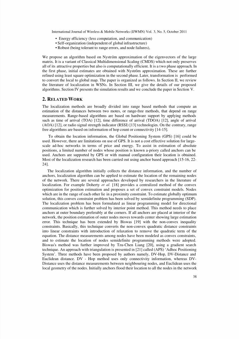
As can be seen from Fig.(3), the RMSE is about 20% for connectivity of 21.6. This graph

shows the RMSE of embeddings after converting it to absolute map with the help of availableanchor nodes. The error goes on decreasing as the connectivity increases. After refinement withleast square optimization the error reduces to 0.81R%. The second and third graph shows the

performance of LwMDS and MDS-MAP (C, R). The error difference between the last twographs is very less, as can be seen from Fig.(3) and Fig.(4).

20 25 30 35 40 45 50 55 600

5

10

15

20

25ANCHORS-4, RANGE ERROR-5%

AVERAGE CONNECTIVITY

R O O T M E A N S Q U A R E E R R O R [ % ]

↓ OVERLAPPED PLOTS

LWMDS

LWMDS-CRMDS-MAP(CR)

Figure 3(a): Average connectivity Vs RMSE with 5% Range error

20 25 30 35 40 45 50 55 60

0.4

0.5

0.6

0.7

0.8

0.9

1ANCHORS-4,RANGE ERROR-5%

R O O T M E A N

S Q U A R E E R R O R [ % ]

AVERAGE C ONNECTIVITY

MDS-MAP(CR)

LWMDS-CR

Figure 3(b): Average connectivity Vs RMSE with 5% Range error

From these two graphs, it is apparent that whenever there is full connectivity, using only thepartial distance matrix [n X (N-n)] also, almost same results are obtained as that of MDS-

MAP(C,R). The main bottleneck of computation in CMDS is of computation of eigen values.The complexity reduces at this step drastically.




45

20 25 30 35 40 45 50 55 600

5

10

15

20

25ANCHORS-6, RANGE E RROR-5%

AVERAGE CONNECTIVITY

R O O T M E A N S Q U A R E E R

R O R

[ % ]

↓ OVERLAPPED PLOTS

LwMDS

LWMDS-R

MDS-MAP(C,R)

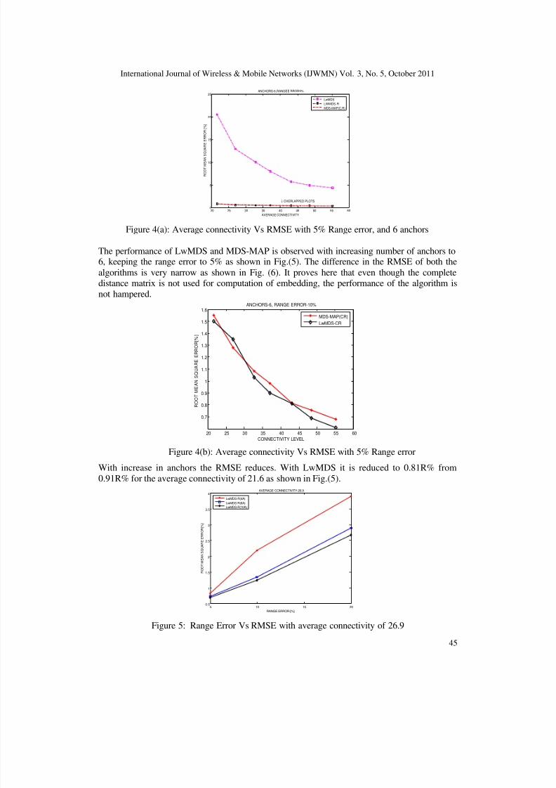
Figure 4(a): Average connectivity Vs RMSE with 5% Range error, and 6 anchors

The performance of LwMDS and MDS-MAP is observed with increasing number of anchors to6, keeping the range error to 5% as shown in Fig.(5). The difference in the RMSE of both the

algorithms is very narrow as shown in Fig. (6). It proves here that even though the completedistance matrix is not used for computation of embedding, the performance of the algorithm is

not hampered.

20 25 30 35 40 45 50 55 60

0.7

0.8

0.9

1

1.1

1.2

1.3

1.4

1.5

1.6ANCHORS-6, RANGE ERROR-10%

CONNECTIVITY LEVEL

R O O T M E A N

S Q U A R E

E R R O R [ % ]

MDS-MAP(CR)

LwMDS-CR

Figure 4(b): Average connectivity Vs RMSE with 5% Range error

With increase in anchors the RMSE reduces. With LwMDS it is reduced to 0.81R% from

0.91R% for the average connectivity of 21.6 as shown in Fig.(5).

5 10 15 200.5

1

1.5

2

2.5

3

3.5

4AVERAGE CONNECTIVITY-26.9

RANGE ERROR-[%]

R O O T M E A N S

Q U A R E E R R O R [ % ]

LwMDS-R(4A)

LwMDS-R(6A)

LwMDS-R(10A)

Figure 5: Range Error Vs RMSE with average connectivity of 26.9




46

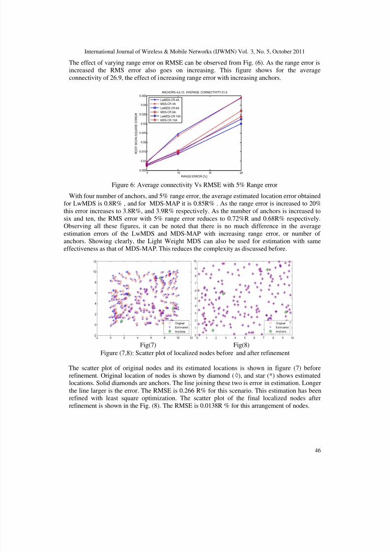
The effect of varying range error on RMSE can be observed from Fig. (6). As the range error isincreased the RMS error also goes on increasing. This figure shows for the average

connectivity of 26.9, the effect of increasing range error with increasing anchors.

5 10 15 200.005

0.01

0.015

0.02

0.025

0.03

0.035

0.04

0.045

ANCHORS-4,6,10, AVERAGE CONNECTIVITY-21.6

RANGE ERROR-[%]

R O O T M E A N S Q U A R E E R R O R

LwMDS-CR-4A

MDS-CR 4A

LwMDS-CR-6A

MDS-CR 6A

LwMDS-CR-10A

MDS-CR 10A

Figure 6: Average connectivity Vs RMSE with 5% Range error

With four number of anchors, and 5% range error, the average estimated location error obtainedfor LwMDS is 0.8R% , and for MDS-MAP it is 0.85R% . As the range error is increased to 20%

this error increases to 3.8R%, and 3.9R% respectively. As the number of anchors is increased to

six and ten, the RMS error with 5% range error reduces to 0.72%R and 0.68R% respectively.Observing all these figures, it can be noted that there is no much difference in the average

estimation errors of the LwMDS and MDS-MAP with increasing range error, or number of anchors. Showing clearly, the Light Weight MDS can also be used for estimation with same

effectiveness as that of MDS-MAP. This reduces the complexity as discussed before.

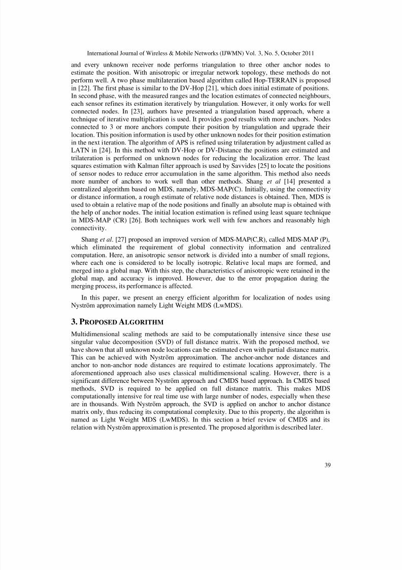
Fig(7) Fig(8)

Figure (7,8): Scatter plot of localized nodes before and after refinement

The scatter plot of original nodes and its estimated locations is shown in figure (7) before

refinement. Original location of nodes is shown by diamond (◊), and star (*) shows estimatedlocations. Solid diamonds are anchors. The line joining these two is error in estimation. Longer

the line larger is the error. The RMSE is 0.266 R% for this scenario. This estimation has beenrefined with least square optimization. The scatter plot of the final localized nodes after

refinement is shown in the Fig. (8). The RMSE is 0.0138R % for this arrangement of nodes.




47

CONCLUSIONS

Multidimensional scaling based localization methods are one of the robust methods in theliterature. However, these methods are computationally intensive. In this paper, we have

proposed a comparatively less complex approximation namely Light weight MDS usingNystrm approximation for finding location estimation of unknown sensor nodes. Through

extensive simulations, we have shown that, even if the distance matrix of anchors is available,with the help of Nystrm approach, the full embedding can be obtained, which reduces the

complexity drastically without much affecting the location estimation.

REFERENCES

[1] N. Alsharabi, L.R. Fa, F. Zing, and M. Ghurab, “Wireless sensor networks of battlefields

hotspot Challenges and solutions”, Proc. Sixth International conf on Modeling and optimization

in Mobile, Adhoc and Wireless Net-works and workshops,2008, pp.192-196

[2] I.Hakala, M. Tikkakoski, and I. Kivela, “Wireless Sensor Network in Environmental

Monitoring - Case Fox,” Proc. of Second International Conference on house Sensor

Technologies and Applications SENSORCOMM '08,25-31 Aug. 2008,pp-202-208

[3] M. Li and L. Yunghao, “Underground Structure Monitoring with Wireless Sensor Networks”,Proc. of International symposium on Information Processing in Sensor Networks , 25-27 April

2007,pp.69-78.

[4] A.S.K Pathan.; L.yung-Woo, and H. C. Seon, “Wireless sensor networks - a security

perspective”, Proc. Of 8th International Conference on Advanced Communication Technology

(ICACT), Sept. 2006.Vol.2 pp. 1048 -1054

[5] W. Wang, V. Srinivasan, B. Wang, and K. C. Chua, “Coverage for target localization in

wireless sensor networks,” in Proc. IPSN , Apr. 2006, pp.118–125

[6] U. Varshney, “Location management for wireless networks: issues and directions”,

International Journal of Mobile Communications, 2003 Vol. 1, Nos.2, pp.91–118.

[7] H. Liu ; Z. Meng and S.Cui,“ A Wireless Sensor Network Prototype for Environmental

Monitoring in Greenhouses”, Proc. of International Conference on Wireless Communications,

Networking and Mobile Computing, 2007. WiCom 2007., 21-25 Sept. 2007 pp- 2344

[8] Z. Guo, Mengchu Zhou, “Optimal Tracking Interval for Predictive Tracking in Wireless Sensor

Network”, IEEE Communication Letters,Vol.9,No9,Sept.2005, pp.805-807[9] M. Estiri , and A. Khademzadeh, “A game-theoretical model for intrusion detection in wireless

sensor networks,” In Proc. of 23rd Canadian Conference on Electrical And Computer

Engineering (CCECE), 2010, 2-5May 2010,pp.1-5

[10] X. Hong, K Xu, and M. Gerla M, “Scalable routing protocols for mobile ad hoc networks”,

IEEE Network Magazine, Vol. 16, No. 4, (2002),pp.11-21

[11] G.Mao, B.Fidan, and Anderson, “Wireless sensor network localization techniques”, The Int.

Journal of Computer and Telecommunications Networking Computer net-works, Vol.51, No.10,

July 2007, pp.2529-2553

[12] P. Xing, H. Yu and Y. Zhang, “An assisting localization method for wireless sensor networks,”

In Proc. Of second International Conference on Mobile Technology, Applications and Systems,

15-17 Nov. 2005, pp.1-6

[13] X. Li, H. Shi and Yi Shang, “A Sorted RSSI Quantization Based Algorithm for Sensor Network

Localization”, In Proc. Of 11th International Conference on Parallel and Distributed Systems,

2005. pp.557 - 563.[14] Y. Shang, W. Ruml, Y.Zhang, M. Fromherz, “Localization from Mere Connectivity” In 4th

ACM international symposium on Mobile and Ad-Hoc Networking & Computing symposium on

Mobile and Ad-Hoc Networking & Computing, (2003), pp. 201–212.

[15] Premaratne, K., Zhang, J. and Doguel, M. , “Location information-aided task-oriented self-

organization of ad hoc sensor systems”, IEEE Sensors Journal, February 2004, Vol. 4, No.

1,pp.85-95




48

[16] S. Kumar, and J. Stokkeland, “Evolution of GPS technology and its subsequent use in

commercial markets”, International Journal of Mobile Communications (2003), Vol. 1, Nos. 1–

2, pp.180–193.

[17] X. Ji and H. Zha, “Multidimensional scaling based sensor positioning algorithms in wireless

sensor networks” , Proceedings of the 1st Annual ACM Conference on Embedded Networked

Sensor Systems, November 2003, pp.328–329.[18] L.Doherty, K.pister, and L. El Ghaoui, “Convex position estimation in wireless sensor

networks,” in IEEE INFOCOM 2001, vol. 3, pp.1655-1663

[19] P.Biswas and Y.Ye, “Semidefinite programming for ad hoc wireless sensor network

localization”, Third international symposium on Information processing in sensor network ,

April 2004, pp.46-54

[20] T. C. Liang, T. C. Wang, and Y. Ye, “A gradient search method to round the semidefinite

programming relaxation solution for adhoc wireless sensor network localization,” Stanford

University, formal report 5, 2004. Availale:http: //www.stanford. edu/-yyye/ formal-report5. Pdf

[21] D.Niculescu and B. Nath, “Adhoc positioning system”, In Proc. of the Global

Telecommunications Conference, San Antonio, CA, USA, (2001). pp. 2926– 2931.

[22] C.Savarese, J.Rabay and K. Langendoen, “Robust positioning algorithms for distributed ad-hoc

wireless sensor networks”, In USENIX Technical Annual conference, June 2002, pp.1-10.

[23] A. Savvides, C. Han, and M. B. Srivastava, “Dynamic fine-grained localization in ad-hoc

networks of sensors”. In Mobile Computing and Networking, 2001, pp. 166-179[24] F.Tian, W.Guo, C. Wang and Q. Gao, “Robust Localization Based on adjustment of

Trilateration Network for Wireless Sensor Networks”, In proc. of 4th Inter-national Conference

on Wireless Communications, networking and Mobile Computing, 2008. WiCOM '08,pp.1-4.

[25] A. Savvides, H. Park, and M. B. Srivastava, "The bits and flops of the n-hop multilateration

primitive for node localization problems," In International Workshop on Sensor Networks

Application, 2002, pp. 112-121.

[26] Y. Shang, W Ruml, Y. Zhang, and M. Fromherz, “Localization from connectivity in sensor

networks”, IEEE Transactions on Parallel and Distributed Systems ,2004,Vol.15 No.11, pp.

961– 974.

[27] Y. Shang and W. Ruml, “Improved MDS-based localization,” in IEEE INFOCOM

2004,pp.2640-2651

[28] J.A.Costa, N.Patwari, andA.O.Hero,III, “Distributed weighted multidimensional scaling for

node localization in sensor networks,” Transactions on Sensor Networks (TOSN) ,February

2006.Vol2(1),pp.1-26[29] H. Lim and J. C. Hou, “Localization for anisotropic sensor networks”, in IEEE INFOCOM

2005,PP.138-149

[30] I. Borg and P. Groenen Modern Multidimensional Scaling, Theory and Applications. Springer-

Verlag,New York, 1997

[31] B. Scholkopf, “The kernel trick for distances”, In Proc. of NIPS,pp-301-307,2000

[32] C. Williams, and M. Seeger, “ Using the Nystrm method to speed up kernel machines”, In

Proc. of Advances in Neural Information Processing Systems,Vol.13,pp.682-688,2001

Documents

Localization in Sensor Network With Nystrom Approximation