Sampling Methods for the Nystrom Method¨

Journal of Machine Learning Research () Submitted ; Published

Sampling Methods for the Nystrom Method

Sanjiv Kumar [email protected]

Google ResearchNew York, NY, USA

Mehryar Mohri [email protected] .EDU

Courant Institute and Google ResearchNew York, NY, USA

Ameet Talwalkar [email protected]

Division of Computer ScienceUniversity of California, BerkeleyBerkeley, CA, USA

Editor: Inderjit Dhillon

Abstract

The Nystrom method is an efficient technique to generate low-rank matrix approxima-tions and is used in several large-scale learning applications. A key aspect of this methodis the procedure according to which columns are sampled fromthe original matrix. In thiswork, we explore the efficacy of a variety offixedandadaptivesampling schemes. Wealso propose a family ofensemble-based sampling algorithms for the Nystrom method.We report results of extensive experiments that provide a detailed comparison of variousfixed and adaptive sampling techniques, and demonstrate theperformance improvementassociated with the ensemble Nystrom method when used in conjunction with either fixedor adaptive sampling schemes. Corroborating these empirical findings, we present a theo-retical analysis of the Nystrom method, providing novel error bounds guaranteeing a betterconvergence rate of the ensemble Nystrom method in comparison to the standard Nystrommethod.

1. Introduction

A common problem in many areas of large-scale machine learning involves deriving a use-ful and efficient approximation of a large matrix. This matrix may be a kernel matrix usedwith support vector machines (Cortes and Vapnik, 1995; Boser et al., 1992), kernel principalcomponent analysis (Scholkopf et al., 1998) or manifold learning (Platt, 2004; Talwalkaret al., 2008). Large matrices also naturally arise in other applications, e.g., clustering, col-laborative filtering, matrix completion, robust PCA, etc. For these large-scale problems,the number of matrix entries can be in the order of tens of thousands to millions, lead-ing to difficulty in operating on, or even storing the matrix.An attractive solution to thisproblem involves using the Nystrom method to generate a low-rank approximation of theoriginal matrix from a subset of its columns (Williams and Seeger, 2000). A key aspect ofthe Nystrom method is the procedure according to which the columns are sampled. This

c© Sanjiv Kumar, Mehryar Mohri and Ameet Talwalkar.

KUMAR , MOHRI AND TALWALKAR

paper presents an analysis of different sampling techniques for the Nystrom method bothempirically and theoretically.1

In the first part of this work, we focus on variousfixedsampling methods. The Nystrommethod was first introduced to the machine learning community (Williams and Seeger,2000) using uniform sampling without replacement, and thisremains the sampling methodmost commonly used in practice (Talwalkar et al., 2008; Fowlkes et al., 2004; de Silvaand Tenenbaum, 2003; Platt, 2004). More recently, the Nystrom method has been theoret-ically analyzed assuming sampling from fixed, non-uniform distributions over the columns(Drineas and Mahoney, 2005; Belabbas and Wolfe, 2009; Mahoney and Drineas, 2009).In this work, we present novel experiments with several real-world datasets comparing theperformance of the Nystrom method when used with uniform versus non-uniform samplingdistributions. Although previous studies have compared uniform and non-uniform distribu-tions in a more restrictive setting (Drineas et al., 2001; Zhang et al., 2008), our results arethe first to compare uniform sampling with the sampling technique for which the Nystrommethod has theoretical guarantees. Our results suggest that uniform sampling, in additionto being more efficient both in time and space, produces more effective approximations. Wefurther show the benefits of sampling without replacement. These empirical findings helpmotivate subsequent theoretical analyses.

The Nystrom method has also been studied empirically and theoretically assuming moresophisticated iterative selection techniques (Smola and Scholkopf, 2000; Fine and Schein-berg, 2002; Bach and Jordan, 2002). In the second part of thiswork, we provide a survey ofadaptive techniques that have been suggested for use with the Nystrom method, and presentan empirical comparison across these algorithms. As part ofthis work, we build upon ideasof Deshpande et al. (2006), in which an adaptive, error-driven sampling technique with rel-ative error bounds was introduced for the related problem ofmatrix projection (see Kumaret al. (2009b) for details). However, this technique requires the full matrix to be availableat each step, and is impractical for large matrices. Hence, we propose a simple and efficientalgorithm that extends the ideas of Deshpande et al. (2006) for adaptive sampling and usesonly a small submatrix at each step. Our empirical results suggest a trade-off between timeand space requirements, as adaptive techniques spend more time to find a concise subset ofinformative columns but provide improved approximation accuracy.

Next, we show that a new family of algorithms based on mixtures of Nystrom approxi-mations,ensemble Nystrom algorithms, yields more accurate low-rank approximations thanthe standard Nystrom method. Moreover, these ensemble algorithms naturally fit within dis-tributed computing environments, where their computational costs are roughly the same asthat of the standard Nystrom method. This issue is of great practical significance given theprevalence of distributed computing frameworks to handle large-scale learning problems.We describe several variants of these algorithms, including one based on simple averagingof p Nystrom solutions, an exponential weighting method, and aregression method whichconsists of estimating the mixture parameters of the ensemble using a few columns sampledfrom the matrix. We also report the results of extensive experiments with these algorithms

1. Portions of this work have previously appeared in the Conference on Artificial Intelligence and Statis-tics (Kumar et al., 2009a), the International Conference onMachine Learning (Kumar et al., 2009b) andAdvances in Neural Information Processing Systems (Kumar et al., 2009c).

2

SAMPLING METHODS FOR THENYSTROM METHOD

on several data sets comparing different variants of the ensemble Nystrom algorithms anddemonstrating the performance improvements gained over the standard Nystrom method.

Finally, we present a theoretical analysis of the Nystrom method, namely bounds on thereconstruction error for both the Frobenius norm and the spectral norm. We first presenta novel bound for the Nystrom method as it is often used in practice, i.e., using uniformsampling without replacement. We next extend this bound to the ensemble Nystrom algo-rithms, and show these novel generalization bounds guarantee a better convergence rate forthese algorithms in comparison to the standard Nystrom method.

The remainder of the paper is organized as follows. Section 2introduces basic def-initions, provides a short survey on related work and gives abrief presentation of theNystrom method. In Section 3, we study various fixed sampling schemes used with theNystrom method. In Section 4, we provide a survey of variousadaptive techniques usedfor sampling-based low-rank approximation and introduce anovel adaptive sampling algo-rithm. Section 5 describes a family of ensemble Nystrom algorithms and presents extensiveexperimental results. We present novel theoretical analysis in Section 6.

2. Preliminaries

Let T ∈ Ra×b be an arbitrary matrix. We defineT(j), j = 1 . . . b, as thejth column

vector ofT, T(i), i = 1 . . . a, as theith row vector ofT and‖·‖ the l2 norm of a vec-tor. Furthermore,T(i:j) refers to theith throughjth columns ofT andT(i:j) refers to theith throughjth rows ofT. If rank(T) = r, we can write the thin Singular Value De-composition (SVD) of this matrix asT = UT ΣTV

⊤T whereΣT is diagonal and contains

the singular values ofT sorted in decreasing order andUT ∈ Ra×r and VT ∈ R

b×r

have orthogonal columns that contain the left and right singular vectors ofT correspond-ing to its singular values. We denote byTk the ‘best’ rank-k approximation toT, i.e.,Tk =argminV∈Ra×b,rank(V)=k‖T −V‖ξ , whereξ ∈ {2, F} and‖·‖2 denotes the spectralnorm and‖·‖F the Frobenius norm of a matrix. We can describe this matrix interms of itsSVD asTk = UT,kΣT,kV

⊤T,k whereΣT,k is a diagonal matrix of the topk singular values

of T andUT,k andVT,k are the matrices formed by the associated left and right singularvectors.

Now letK ∈ Rn×n be a symmetric positive semidefinite (SPSD) kernel or Gram matrix

with rank(K) = r ≤ n, i.e. a symmetric matrix for which there exists anX ∈ RN×n such

that K = X⊤X. We will write the SVD ofK as K = UΣU

⊤, where the columnsof U are orthogonal andΣ = diag(σ1, . . . , σr) is diagonal. The pseudo-inverse ofK

is defined asK+ =∑r

t=1 σ−1t U

(t)U

(t)⊤, andK+ = K

−1 whenK is full rank. For

k < r, Kk =∑k

t=1 σtU(t)

U(t)⊤ = UkΣkU

⊤k is the ‘best’ rank-k approximation toK,

i.e., Kk = argminK′∈Rn×n,rank(K′)=k‖K − K′‖ξ∈{2,F}, with ‖K − Kk‖2 = σk+1 and

‖K−Kk‖F =√∑r

t=k+1 σ2t (Golub and Loan, 1983).

We will be focusing on generating an approximationK of K based on a sample ofl ≪ n of its columns. For now, we assume that the sample ofl columns is given to us,though the focus of this paper will be on various methods for selecting columns. LetCdenote then× l matrix formed by these columns andW the l × l matrix consisting of theintersection of thesel columns with the correspondingl rows ofK. Note thatW is SPSD

3


sinceK is SPSD. Without loss of generality, the columns and rows ofK can be rearrangedbased on this sampling so thatK andC be written as follows:

K =

[W K

⊤21

K21 K22

]and C =

[W

K21

]. (1)

2.1 Nystrom method

The Nystrom method usesW andC from (1) to approximateK. Assuming a uniformsampling of the columns, the Nystrom method generates a rank-k approximationK of K

for k < n defined by:K

nysk = CW

+k C

⊤ ≈ K, (2)

whereWk is the bestk-rank approximation ofW with respect to the spectral or Frobeniusnorm andW+

k denotes the pseudo-inverse ofWk. The Nystrom method thus approximatesthe topk singular values (Σk) and singular vectors (Uk) of K as:

Σnysk =

(nl

)ΣW,k and U

nysk =

√l

nCUW,kΣ

+W,k. (3)

When k = l (or more generally, wheneverk ≥ rank(C)), this approximation perfectlyreconstructs three blocks ofK, andK22 is approximated by the Schur Complement ofW

in K:

Knysl = CW

+C

⊤ =

[W K

⊤21

K21 K21W+K21

]. (4)

Since the running time complexity of SVD onW is in O(kl2) and matrix multiplicationwith C takesO(kln), the total complexity of the Nystrom approximation computation is inO(kln).

2.2 Related Work

There has been a wide array of work on low-rank matrix approximation within the nu-merical linear algebra and computer science communities, much of which has been in-spired by the celebrated result of Johnson and Lindenstrauss (Johnson and Lindenstrauss,1984), which showed that random low-dimensional embeddings preserve Euclidean geom-etry. This result has led to a family of random projection algorithms, which involves pro-jecting the original matrix onto a random low-dimensional subspace (Papadimitriou et al.,1998; Indyk, 2006; Liberty, 2009). Alternatively, SVD can be used to generate ‘optimal’low-rank matrix approximations, as mentioned earlier. However, both the random projec-tion and the SVD algorithms involve storage and operating onthe entire input matrix. SVDis more computationally expensive than random projection methods, though neither are lin-ear inn in terms of time and space complexity. When dealing with sparse matrices, thereexist less computationally intensive techniques such as Jacobi, Arnoldi, Hebbian and morerecent randomized methods (Golub and Loan, 1983; Gorrell, 2006; Rokhlin et al., 2009;Halko et al., 2009) for generating low-rank approximations. These methods require com-putation of matrix-vector products and thus require operating on every non-zero entry ofthe matrix, which may not be suitable for large, dense matrices. Matrix sparsification algo-rithms (Achlioptas and Mcsherry, 2007; Arora et al., 2006),as the name suggests, attempt

4


to sparsify dense matrices to speed up future storage and computational burdens, thoughthey too require storage of the input matrix and exhibit superlinear processing time.

Alternatively, sampling-based approaches can be used to generate low-rank approxi-mations. Research in this area dates back to classical theoretical results that show, forany arbitrary matrix, the existence of a subset ofk columns for which the error in matrixprojection (as defined in (Kumar et al., 2009b)) can be bounded relative to the optimalrank-k approximation of the matrix (Ruston, 1962). Deterministicalgorithms such as rank-revealing QR (Gu and Eisenstat, 1996) can achieve nearly optimal matrix projection errors.More recently, research in the theoretical computer science community has been aimed atderiving bounds on matrix projection error using sampling-based approximations, includ-ing additive error bounds using sampling distributions based on the squaredL2 norms ofthe columns (Frieze et al., 1998; Drineas et al., 2006a; Rudelson and Vershynin, 2007); rel-ative error bounds using adaptive sampling techniques (Deshpande et al., 2006; Har-peled,2006); and, relative error bounds based on distributions derived from the singular vectorsof the input matrix, in work related to the column-subset selection problem (Drineas et al.,2008; Boutsidis et al., 2009). These sampling-based approximations all require visitingevery entry of the matrix in order to get good performance guarantees for any matrix. How-ever, as discussed in (Kumar et al., 2009b), the task of matrix projection involves projectingthe input matrix onto a low-rank subspace, which requires superlinear time and space withrespect ton and is not always feasible for large-scale matrices.

There does exist, however, another class of sampling-basedapproximation algorithmsthat only store and operate on a subset of the original matrix. For arbitrary rectangular ma-trices, these algorithms are known as ‘CUR’ approximations(the name ‘CUR’ correspondsto the three low-rank matrices whose product is an approximation to the original matrix).The theoretical performance of CUR approximations has beenanalyzed using a variety ofsampling schemes, although the column-selection processes associated with these analysesoften require operating on the entire input matrix (Goreinov et al., 1997; Stewart, 1999;Drineas et al., 2008; Mahoney and Drineas, 2009).

In the context of symmetric positive semidefinite matrices,the Nystrom method is acommonly used algorithm to efficiently generate low-rank approximations. The Nystrommethod was initially introduced as a quadrature method for numerical integration, used toapproximate eigenfunction solutions (Nystrom, 1928; Baker, 1977). More recently, it waspresented in Williams and Seeger (2000) to speed up kernel algorithms and has been stud-ied theoretically using a variety of sampling schemes (Smola and Scholkopf, 2000; Drineasand Mahoney, 2005; Zhang et al., 2008; Zhang and Kwok, 2009; Kumar et al., 2009a,b,c;Belabbas and Wolfe, 2009; Belabbas and Wolfe, 2009; Cortes et al., 2010; Talwalkar andRostamizadeh, 2010). It has also been used for a variety of machine learning tasks rangingfrom manifold learning to image segmentation (Platt, 2004;Fowlkes et al., 2004; Talwalkaret al., 2008). A closely related algorithm, known as the Incomplete Cholesky Decom-position (Fine and Scheinberg, 2002; Bach and Jordan, 2002,2005), can also be viewedas a specific sampling technique associated with the Nystrom method (Bach and Jordan,2005). As noted by Candes and Recht (2009); Talwalkar and Rostamizadeh (2010), theNystrom approximation is related to the problem of matrix completion (Candes and Recht,2009; Candes and Tao, 2009), which attempts to complete a low-rank matrix from a ran-dom sample of its entries. However, the matrix completion attempts to impute a low-rank

5


matrix from a subset of (possibly perturbed) matrix entries, rather than a subset of matrixcolumns. This problem is related to, yet distinct from the Nystrom method and sampling-based low-rank approximation algorithms in general, that deal with full-rank matrices thatare amenable to low-rank approximation. Furthermore, whenwe have access to the under-lying kernel function that generates the kernel matrix of interest, we can generate matrixentries on-the-fly as desired, providing us with more flexibility accessing the original ma-trix.

3. Fixed Sampling

Since the Nystrom method operates on a small subset ofK, i.e.,C, the selection of columnscan significantly influence the accuracy of the approximation. In the remainder of the pa-per, we will discuss various sampling options that aim to select informative columns fromK. We begin with the most common class of sampling techniques that select columns us-ing a fixed probability distribution. The most basic sampling technique involvesuniformsampling of the columns. Alternatively, theith column can be sampled non-uniformly withweight proportional to either its corresponding diagonal elementKii (diagonal sampling) ortheL2 norm of the column (column-norm sampling) (Drineas et al., 2006b; Drineas and Ma-honey, 2005). There are additional computational costs associated with these non-uniformsampling methods:O(n) time and space requirements for diagonal sampling andO(n2)time and space for column-norm sampling. These non-uniformsampling techniques areoften presented using sampling with replacement to simplify theoretical analysis. Column-norm sampling has been used to analyze a general SVD approximation algorithm. Further,diagonal sampling with replacement was used by Drineas and Mahoney (2005) and Belab-bas and Wolfe (2009) to bound the reconstruction error of theNystrom method.2 In Drineasand Mahoney (2005) however, the authors suggest that column-norm sampling would be abetter sampling assumption for the analysis of the Nystrommethod. We also note that Be-labbas and Wolfe (2009) proposed a family of ‘annealed determinantal’ distributions forwhich multiplicative bounds on reconstruction error were derived. However, in practice,these distributions cannot be efficiently computed except for special cases coinciding withuniform and column-norm sampling. Similarly, although Mahoney and Drineas (2009)present multiplicative bounds for the CUR decomposition (which is quite similar to theNystrom method) when sampling from a distribution over thecolumns based on ‘leveragescores,’ these scores cannot be efficiently computed in practice for large-scale applications.

In the remainder of this section we present novel experimental results comparing theperformance of these fixed sampling methods on several data sets. Previous studies havecompared uniform and non-uniform in a more restrictive setting, using fewer types of ker-nels and focusing only on column-norm sampling (Drineas et al., 2001; Zhang et al., 2008).However, in this work, we provide the first comparison that includes diagonal sampling,which is the non-uniform distribution that is most scalablefor large-scale applications andwhich has been used in some theoretical analyses of the Nystrom method.

2. Although Drineas and Mahoney (2005) claim to weight each column proportionally toK2

ii, they in fact usethe diagonal sampling we present in this work, i.e., weightsproportional toKii (Drineas, 2008).

6


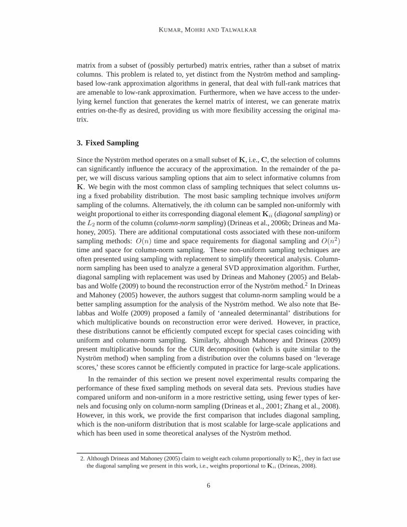
Name Type n d KernelPIE-2.7K faces (profile) 2731 2304 linearPIE-7K faces (front) 7412 2304 linearMNIST digit images 4000 784 linear

ESS proteins 4728 16 RBFABN abalones 4177 8 RBF

Table 1: Description of the datasets and kernels used in fixedand adaptive sampling experi-ments (Sim et al., 2002; LeCun and Cortes, 1998; Gustafson etal., 2006; Asuncionand Newman, 2007). ‘d’ denotes the number of features in input space.

3.1 Datasets

We used 5 datasets from a variety of applications, e.g., computer vision and biology, asdescribed in Table 1. SPSD kernel matrices were generated bymean centering the datasetsand applying either a linear kernel or RBF kernel. The diagonals (respectively columnnorms) of these kernel matrices were used to calculate diagonal (respectively column-norm)distributions. Note that the diagonal distribution equalsthe uniform distribution for RBFkernels since diagonal entries of RBF kernel matrices always equal one.

3.2 Experiments

We used the datasets described in the previous section to test the approximation accuracy foreach sampling method. Low-rank approximations ofK were generated using the Nystrommethod along with these sampling methods, and we measured the accuracy of reconstruc-tion relative to the optimal rank-k approximation,Kk, as:

relative accuracy=‖K−Kk‖F‖K− Kk‖F

× 100. (5)

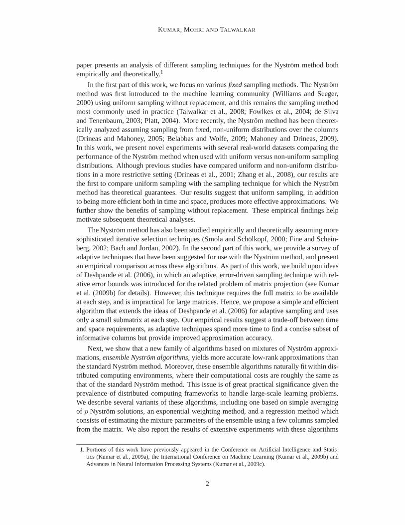
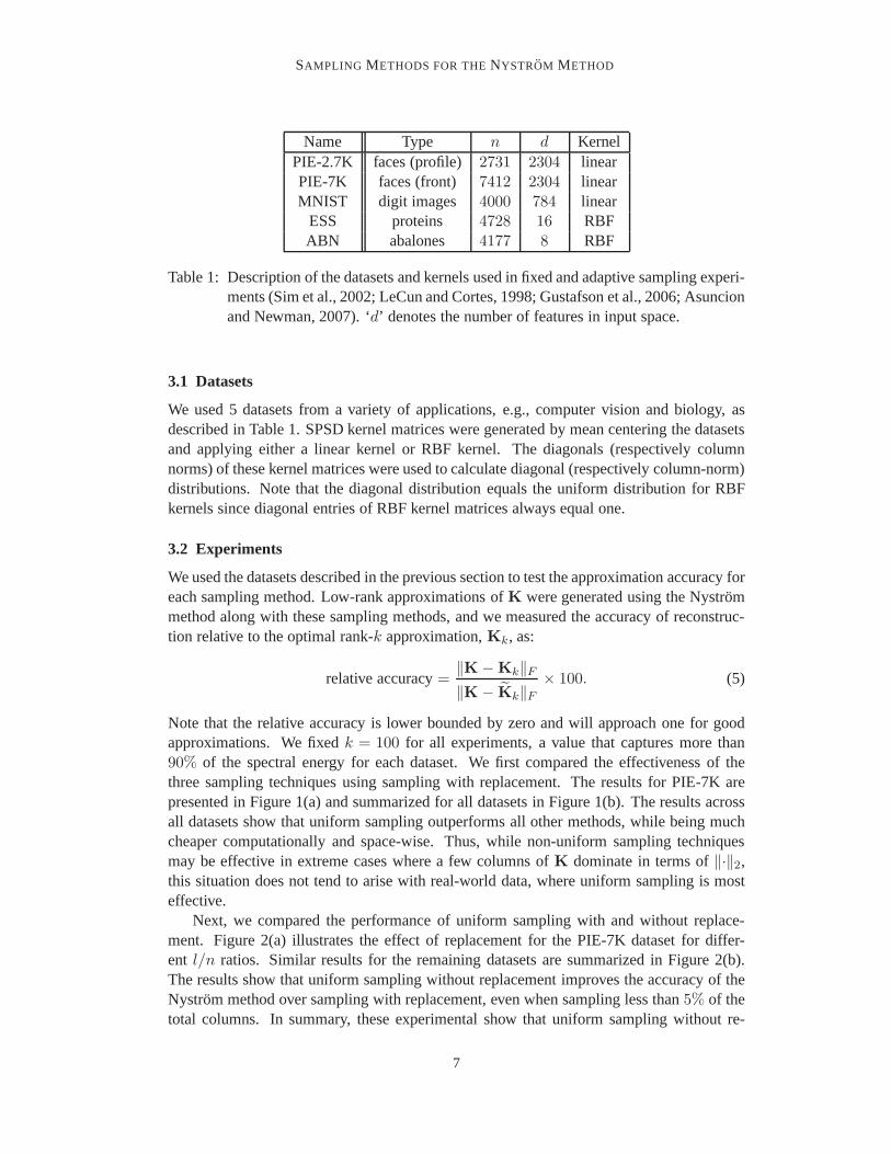
Note that the relative accuracy is lower bounded by zero and will approach one for goodapproximations. We fixedk = 100 for all experiments, a value that captures more than90% of the spectral energy for each dataset. We first compared theeffectiveness of thethree sampling techniques using sampling with replacement. The results for PIE-7K arepresented in Figure 1(a) and summarized for all datasets in Figure 1(b). The results acrossall datasets show that uniform sampling outperforms all other methods, while being muchcheaper computationally and space-wise. Thus, while non-uniform sampling techniquesmay be effective in extreme cases where a few columns ofK dominate in terms of‖·‖2,this situation does not tend to arise with real-world data, where uniform sampling is mosteffective.

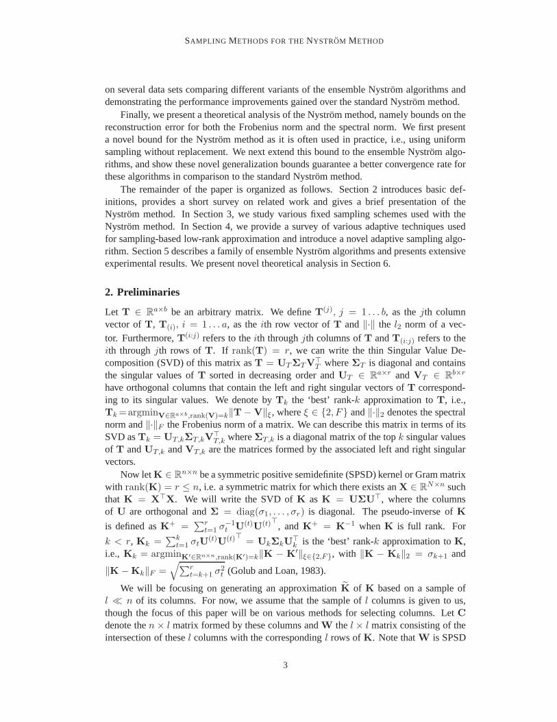
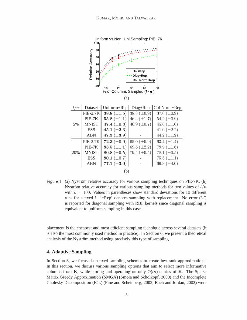
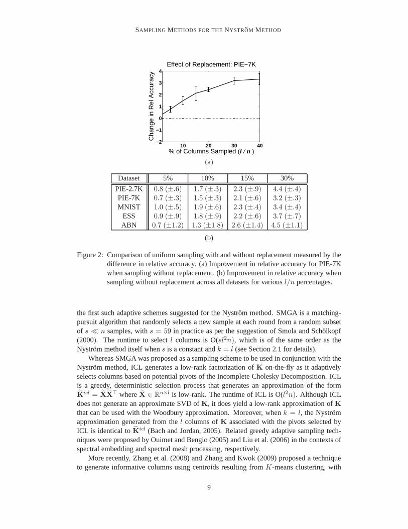
Next, we compared the performance of uniform sampling with and without replace-ment. Figure 2(a) illustrates the effect of replacement forthe PIE-7K dataset for differ-ent l/n ratios. Similar results for the remaining datasets are summarized in Figure 2(b).The results show that uniform sampling without replacementimproves the accuracy of theNystrom method over sampling with replacement, even when sampling less than5% of thetotal columns. In summary, these experimental show that uniform sampling without re-

7


10 20 30 40 5040

50

60

70

80

90

100

% of Columns Sampled (l / n )R

elat

ive

Acc

urac

y

Uniform vs Non−Uni Sampling: PIE−7K

Uni+RepDiag+RepCol−Norm+Rep

(a)

l/n Dataset Uniform+Rep Diag+Rep Col-Norm+RepPIE-2.7K 38.8 (±1.5) 38.3 (±0.9) 37.0 (±0.9)PIE-7K 55.8 (±1.1) 46.4 (±1.7) 54.2 (±0.9)

5% MNIST 47.4 (±0.8) 46.9 (±0.7) 45.6 (±1.0)ESS 45.1 (±2.3) - 41.0 (±2.2)ABN 47.3 (±3.9) - 44.2 (±1.2)

PIE-2.7K 72.3 (±0.9) 65.0 (±0.9) 63.4 (±1.4)PIE-7K 83.5 (±1.1) 69.8 (±2.2) 79.9 (±1.6)

20% MNIST 80.8 (±0.5) 79.4 (±0.5) 78.1 (±0.5)ESS 80.1 (±0.7) - 75.5 (±1.1)ABN 77.1 (±3.0) - 66.3 (±4.0)

(b)

Figure 1: (a) Nystrom relative accuracy for various sampling techniques on PIE-7K. (b)Nystrom relative accuracy for various sampling methods for two values ofl/nwith k = 100. Values in parentheses show standard deviations for10 differentruns for a fixedl. ‘+Rep’ denotes sampling with replacement. No error (‘-’)is reported for diagonal sampling with RBF kernels since diagonal sampling isequivalent to uniform sampling in this case.

placement is the cheapest and most efficient sampling technique across several datasets (itis also the most commonly used method in practice). In Section 6, we present a theoreticalanalysis of the Nystrom method using precisely this type ofsampling.

4. Adaptive Sampling

In Section 3, we focused on fixed sampling schemes to create low-rank approximations.In this section, we discuss various sampling options that aim to select more informativecolumns fromK, while storing and operating on only O(ln) entries ofK. The SparseMatrix Greedy Approximation (SMGA) (Smola and Scholkopf,2000) and the IncompleteCholesky Decomposition (ICL) (Fine and Scheinberg, 2002; Bach and Jordan, 2002) were

8


10 20 30 40−2

−1

0

1

2

3

4Effect of Replacement: PIE−7K

% of Columns Sampled (l / n )C

hang

e in

Rel

Acc

urac

y

(a)

Dataset 5% 10% 15% 30%

PIE-2.7K 0.8 (±.6) 1.7 (±.3) 2.3 (±.9) 4.4 (±.4)PIE-7K 0.7 (±.3) 1.5 (±.3) 2.1 (±.6) 3.2 (±.3)MNIST 1.0 (±.5) 1.9 (±.6) 2.3 (±.4) 3.4 (±.4)

ESS 0.9 (±.9) 1.8 (±.9) 2.2 (±.6) 3.7 (±.7)ABN 0.7 (±1.2) 1.3 (±1.8) 2.6 (±1.4) 4.5 (±1.1)

(b)

Figure 2: Comparison of uniform sampling with and without replacement measured by thedifference in relative accuracy. (a) Improvement in relative accuracy for PIE-7Kwhen sampling without replacement. (b) Improvement in relative accuracy whensampling without replacement across all datasets for various l/n percentages.

the first such adaptive schemes suggested for the Nystrom method. SMGA is a matching-pursuit algorithm that randomly selects a new sample at eachround from a random subsetof s ≪ n samples, withs = 59 in practice as per the suggestion of Smola and Scholkopf(2000). The runtime to selectl columns is O(sl2n), which is of the same order as theNystrom method itself whens is a constant andk = l (see Section 2.1 for details).

Whereas SMGA was proposed as a sampling scheme to be used in conjunction with theNystrom method, ICL generates a low-rank factorization ofK on-the-fly as it adaptivelyselects columns based on potential pivots of the IncompleteCholesky Decomposition. ICLis a greedy, deterministic selection process that generates an approximation of the formK

icl = XX⊤ whereX ∈ R

n×l is low-rank. The runtime of ICL is O(l2n). Although ICLdoes not generate an approximate SVD ofK, it does yield a low-rank approximation ofK

that can be used with the Woodbury approximation. Moreover,whenk = l, the Nystromapproximation generated from thel columns ofK associated with the pivots selected byICL is identical toK

icl (Bach and Jordan, 2005). Related greedy adaptive sampling tech-niques were proposed by Ouimet and Bengio (2005) and Liu et al. (2006) in the contexts ofspectral embedding and spectral mesh processing, respectively.

More recently, Zhang et al. (2008) and Zhang and Kwok (2009) proposed a techniqueto generate informative columns using centroids resultingfrom K-means clustering, with

9


K = l. This algorithm, which uses out-of-sample extensions to generate a set ofl represen-tative columns ofK, has been shown to give good empirical accuracy (Zhang et al., 2008).Finally, an adaptive sampling technique with strong theoretical foundations (adaptive-full)was proposed in Deshpande et al. (2006). It requires a full pass throughK in each iterationand is thus inefficient for largeK. In the remainder of this section, we first propose a noveladaptive technique that extends the ideas of Deshpande et al. (2006) and then present em-pirical results comparing the performance of this new algorithm with uniform sampling aswell as SMGA, ICL,K-means and theadaptive-fulltechniques.

Input : n × n SPSD matrix (K), number columns to be chosen (l), initial distribution overcolumns (P0), number columns selected at each iteration (s)Output : l indices corresponding to columns ofK

SAMPLE-ADAPTIVE(K, n, l, P0 , s)

1 R← set ofs indices sampled according toP0

2 t← ls − 1 � number of iterations

3 for i ∈ [1 . . . t] do4 Pi ← UPDATE-PROBABILITY-FULL (R)5 Ri ← set ofs indices sampled according toPi

6 R← R ∪Ri

7 return R

UPDATE-PROBABILITY-FULL(R)

1 C′ ← columns ofK corresponding to indices inR

2 UC′ ← left singular vectors ofC′

3 E← K−UC′U⊤C′K

4 for j ∈ [1 . . . n] do5 if j ∈ R then6 Pj ← 07 else Pj ← ||Ej ||228 P ← P

||P ||29 return P

Figure 3: The adaptive sampling technique (Deshpande et al., 2006) that operates on theentire matrixK to compute the probability distribution over columns at eachadaptive step.

4.1 Adaptive Nystrom sampling

Instead of sampling alll columns from a fixed distribution, adaptive sampling alternates be-tween selecting a set of columns and updating the distribution over all the columns. Startingwith an initial distribution over the columns,s < l columns are chosen to form a submatrixC

′. The probabilities are then updated as a function of previously chosen columns ands

10


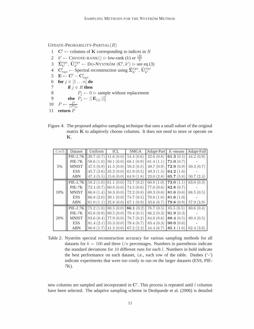
UPDATE-PROBABILITY-PARTIAL (R)

1 C′ ← columns ofK corresponding to indices inR

2 k′ ← CHOOSE-RANK() � low-rank (k) or |R|2

3 Σnysk′ , U

nysk′ ← DO-NYSTROM (C′, k′) � see eq (3)

4 C′nys ← Spectral reconstruction usingΣnys

k′ , Unysk′

5 E← C′ −C

′nys

6 for j ∈ [1 . . . n] do7 if j ∈ R then8 Pj ← 0 � sample without replacement9 else Pj ← ||E(j) ||22

10 P ← P||P ||2

11 return P

Figure 4: The proposed adaptive sampling technique that uses a small subset of the originalmatrix K to adaptively choose columns. It does not need to store or operate onK.

l/n% Dataset Uniform ICL SMGA Adapt-Part K-means Adapt-FullPIE-2.7K 39.7 (0.7) 41.6 (0.0) 54.4 (0.6) 42.6 (0.8) 61.3 (0.5) 44.2 (0.9)PIE-7K 58.6 (1.0) 50.1 (0.0) 68.1 (0.9) 61.4 (1.1) 71.0 (0.7) -

5% MNIST 47.5 (0.9) 41.5 (0.0) 59.2 (0.5) 49.7 (0.9) 72.9 (0.9) 50.3 (0.7)ESS 45.7 (2.6) 25.2 (0.0) 61.9 (0.5) 49.3 (1.5) 64.2 (1.6) -ABN 47.4 (5.5) 15.6 (0.0) 64.9 (1.8) 23.0 (2.8) 65.7 (5.8) 50.7 (2.4)

PIE-2.7K 58.2 (1.0) 61.1 (0.0) 72.7 (0.2) 60.8 (1.0) 73.0 (1.1) 63.0 (0.3)PIE-7K 72.4 (0.7) 60.8 (0.0) 74.5 (0.6) 77.0 (0.6) 82.8 (0.7) -

10% MNIST 66.8 (1.4) 58.3 (0.0) 72.2 (0.8) 69.3 (0.6) 81.6 (0.6) 68.5 (0.5)ESS 66.8 (2.0) 39.1 (0.0) 74.7 (0.5) 70.0 (1.0) 81.6 (1.0) -ABN 61.0 (1.1) 25.8 (0.0) 67.1 (0.9) 33.6 (6.7) 79.8 (0.9) 57.9 (3.9)

PIE-2.7K 75.2 (1.0) 80.5 (0.0) 86.1 (0.2) 78.7 (0.5) 85.5 (0.5) 80.6 (0.4)PIE-7K 85.6 (0.9) 69.5 (0.0) 79.4 (0.5) 86.2 (0.3) 91.9 (0.3) -

20% MNIST 83.6 (0.4) 77.9 (0.0) 78.7 (0.2) 84.0 (0.6) 88.4 (0.5) 80.4 (0.5)ESS 81.4 (2.1) 55.3 (0.0) 79.4 (0.7) 83.4 (0.3) 90.0 (0.6) -ABN 80.8 (1.7) 41.2 (0.0) 67.2 (2.2) 44.4 (6.7) 85.1 (1.6) 62.4 (3.6)

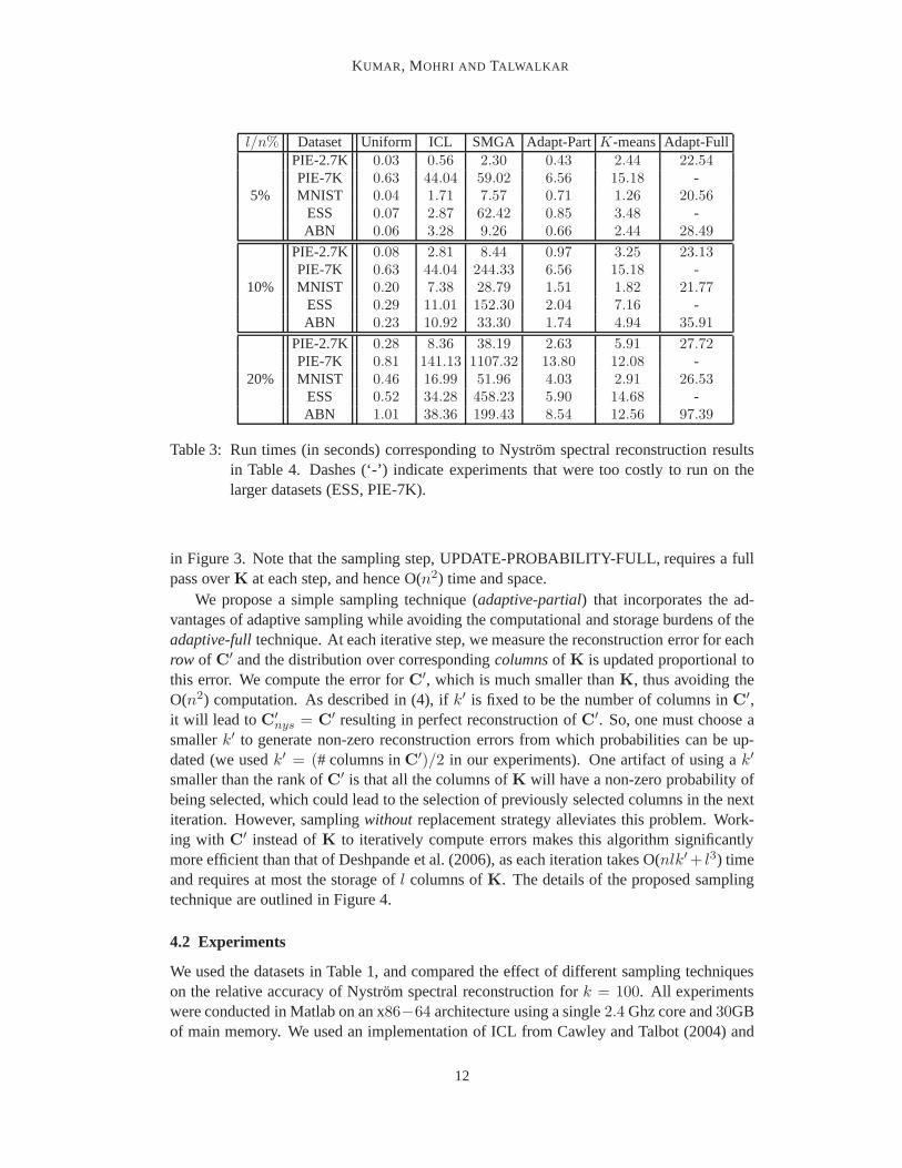
Table 2: Nystrom spectral reconstruction accuracy for various sampling methods for alldatasets fork = 100 and threel/n percentages. Numbers in parenthesis indicatethe standard deviations for10 different runs for eachl. Numbers in bold indicatethe best performance on each dataset, i.e., each row of the table. Dashes (‘-’)indicate experiments that were too costly to run on the larger datasets (ESS, PIE-7K).

new columns are sampled and incorporated inC′. This process is repeated untill columns

have been selected. The adaptive sampling scheme in Deshpande et al. (2006) is detailed

11


l/n% Dataset Uniform ICL SMGA Adapt-PartK-meansAdapt-FullPIE-2.7K 0.03 0.56 2.30 0.43 2.44 22.54PIE-7K 0.63 44.04 59.02 6.56 15.18 -

5% MNIST 0.04 1.71 7.57 0.71 1.26 20.56ESS 0.07 2.87 62.42 0.85 3.48 -ABN 0.06 3.28 9.26 0.66 2.44 28.49

PIE-2.7K 0.08 2.81 8.44 0.97 3.25 23.13PIE-7K 0.63 44.04 244.33 6.56 15.18 -

10% MNIST 0.20 7.38 28.79 1.51 1.82 21.77ESS 0.29 11.01 152.30 2.04 7.16 -ABN 0.23 10.92 33.30 1.74 4.94 35.91

PIE-2.7K 0.28 8.36 38.19 2.63 5.91 27.72PIE-7K 0.81 141.13 1107.32 13.80 12.08 -

20% MNIST 0.46 16.99 51.96 4.03 2.91 26.53ESS 0.52 34.28 458.23 5.90 14.68 -ABN 1.01 38.36 199.43 8.54 12.56 97.39

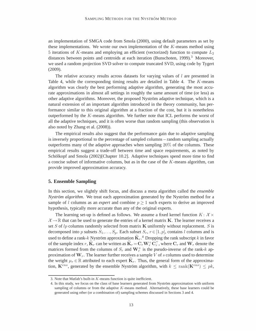
Table 3: Run times (in seconds) corresponding to Nystrom spectral reconstruction resultsin Table 4. Dashes (‘-’) indicate experiments that were too costly to run on thelarger datasets (ESS, PIE-7K).

in Figure 3. Note that the sampling step, UPDATE-PROBABILITY-FULL, requires a fullpass overK at each step, and hence O(n2) time and space.

We propose a simple sampling technique (adaptive-partial) that incorporates the ad-vantages of adaptive sampling while avoiding the computational and storage burdens of theadaptive-fulltechnique. At each iterative step, we measure the reconstruction error for eachrow of C′ and the distribution over correspondingcolumnsof K is updated proportional tothis error. We compute the error forC′, which is much smaller thanK, thus avoiding theO(n2) computation. As described in (4), ifk′ is fixed to be the number of columns inC′,it will lead to C

′nys = C

′ resulting in perfect reconstruction ofC′. So, one must choose a

smallerk′ to generate non-zero reconstruction errors from which probabilities can be up-dated (we usedk′ = (# columns inC′)/2 in our experiments). One artifact of using ak′

smaller than the rank ofC′ is that all the columns ofK will have a non-zero probability ofbeing selected, which could lead to the selection of previously selected columns in the nextiteration. However, samplingwithout replacement strategy alleviates this problem. Work-ing with C

′ instead ofK to iteratively compute errors makes this algorithm significantlymore efficient than that of Deshpande et al. (2006), as each iteration takes O(nlk′ + l3) timeand requires at most the storage ofl columns ofK. The details of the proposed samplingtechnique are outlined in Figure 4.

4.2 Experiments

We used the datasets in Table 1, and compared the effect of different sampling techniqueson the relative accuracy of Nystrom spectral reconstruction for k = 100. All experimentswere conducted in Matlab on an x86−64 architecture using a single2.4 Ghz core and30GBof main memory. We used an implementation of ICL from Cawley and Talbot (2004) and

12


an implementation of SMGA code from Smola (2000), using default parameters as set bythese implementations. We wrote our own implementation of theK-means method using5 iterations ofK-means and employing an efficient (vectorized) function to computeL2

distances between points and centroids at each iteration (Bunschoten, 1999).3 Moreover,we used a random projection SVD solver to compute truncated SVD, using code by Tygert(2009).

The relative accuracy results across datasets for varying values ofl are presented inTable 4, while the corresponding timing results are detailed in Table 4. TheK-meansalgorithm was clearly the best performing adaptive algorithm, generating the most accu-rate approximations in almost all settings in roughly the same amount of time (or less) asother adaptive algorithms. Moreover, the proposed Nystrom adaptive technique, which is anatural extension of an important algorithm introduced in the theory community, has per-formance similar to this original algorithm at a fraction ofthe cost, but it is nonethelessoutperformed by theK-means algorithm. We further note that ICL performs the worst ofall the adaptive techniques, and it is often worse than random sampling (this observation isalso noted by Zhang et al. (2008)).

The empirical results also suggest that the performance gain due to adaptive samplingis inversely proportional to the percentage of sampled columns – random sampling actuallyoutperforms many of the adaptive approaches when sampling20% of the columns. Theseempirical results suggest a trade-off between time and space requirements, as noted byScholkopf and Smola (2002)[Chapter 10.2]. Adaptive techniques spend more time to finda concise subset of informative columns, but as in the case oftheK-means algorithm, canprovide improved approximation accuracy.

5. Ensemble Sampling

In this section, we slightly shift focus, and discuss a meta algorithm called theensembleNystrom algorithm. We treat each approximation generated by the Nystrom method for asample ofl columns as anexpertand combinep ≥ 1 such experts to derive an improvedhypothesis, typically more accurate than any of the original experts.

The learning set-up is defined as follows. We assume a fixed kernel functionK : X ×X→R that can be used to generate the entries of a kernel matrixK. The learner receives asetS of lp columns randomly selected from matrixK uniformly without replacement.S isdecomposed intop subsetsS1,. . ., Sp. Each subsetSr, r∈ [1, p], containsl columns and isused to define a rank-k Nystrom approximationKr.4 Dropping the rank subscriptk in favorof the sample indexr, Kr can be written asKr =CrW

+r C

⊤r , whereCr andWr denote the

matrices formed from the columns ofSr andW+r is the pseudo-inverse of the rank-k ap-

proximation ofWr. The learner further receives a sampleV of s columns used to determinethe weightµr ∈R attributed to each expertKr. Thus, the general form of the approxima-tion, Kens, generated by the ensemble Nystrom algorithm, withk ≤ rank(Kens) ≤ pk,

3. Note that Matlab’s built-inK-means function is quite inefficient.4. In this study, we focus on the class of base learners generated from Nystrom approximation with uniform

sampling of columns or from the adaptiveK-means method. Alternatively, these base learners could begenerated using other (or a combination of) sampling schemes discussed in Sections 3 and 4.

13


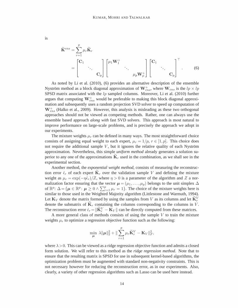
is

Kens =

p∑

r=1

µrKr

=

C1

. . .Cp

µ1W

+1

. . .µpW

+p

C1

. . .Cp

⊤

. (6)

As noted by Li et al. (2010), (6) provides an alternative description of the ensembleNystrom method as a block diagonal approximation ofW

+ens, whereWens is thelp × lp

SPSD matrix associated with thelp sampled columns. Moreover, Li et al. (2010) furtherargues that computingW+

ens would be preferable to making this block diagonal approxi-mation and subsequently uses a random projection SVD solverto speed up computation ofW

+ens (Halko et al., 2009). However, this analysis is misleading as these two orthogonal

approaches should not be viewed as competing methods. Rather, one can always use theensemble based approachalong with fast SVD solvers. This approach is most natural toimprove performance on large-scale problems, and is precisely the approach we adopt inour experiments.

The mixture weightsµr can be defined in many ways. The most straightforward choiceconsists of assigning equal weight to each expert,µr = 1/p, r ∈ [1, p]. This choice doesnot require the additional sampleV , but it ignores the relative quality of each Nystromapproximation. Nevertheless, this simpleuniform methodalready generates a solution su-perior to any one of the approximationsKr used in the combination, as we shall see in theexperimental section.

Another method, theexponential weight method, consists of measuring the reconstruc-tion error ǫr of each expertKr over the validation sampleV and defining the mixtureweight asµr = exp(−ηǫr)/Z, whereη > 0 is a parameter of the algorithm andZ a nor-malization factor ensuring that the vectorµ = (µ1, . . . , µp) belongs to the unit simplex∆of R

p: ∆={µ ∈ Rp : µ ≥ 0 ∧

∑pr=1 µr = 1}. The choice of the mixture weights here is

similar to those used in the Weighted Majority algorithm (Littlestone and Warmuth, 1994).Let KV denote the matrix formed by using the samples fromV as its columns and letKV

r

denote the submatrix ofKr containing the columns corresponding to the columns inV .The reconstruction errorǫr =‖KV

r −KV ‖ can be directly computed from these matrices.A more general class of methods consists of using the sampleV to train the mixture

weightsµr to optimize a regression objective function such as the following:

minµ

λ‖µ‖22 + ‖p∑

r=1

µrKVr −KV ‖2F ,

whereλ>0. This can be viewed as a ridge regression objective functionand admits a closedform solution. We will refer to this method as theridge regression method. Note that toensure that the resulting matrix is SPSD for use in subsequent kernel-based algorithms, theoptimization problem must be augmented with standard non-negativity constraints. This isnot necessary however for reducing the reconstruction error, as in our experiments. Also,clearly, a variety of other regression algorithms such as Lasso can be used here instead.

14


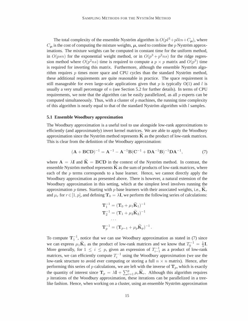
The total complexity of the ensemble Nystrom algorithm isO(pl3+plkn+Cµ), whereCµ is the cost of computing the mixture weights,µ, used to combine thepNystrom approx-imations. The mixture weights can be computed in constant time for the uniform method,in O(psn) for the exponential weight method, or inO(p3 + p2ns) for the ridge regres-sion method whereO(p2ns) time is required to compute ap × p matrix andO(p3) timeis required for inverting this matrix. Furthermore, although the ensemble Nystrom algo-rithm requiresp times more space and CPU cycles than the standard Nystrom method,these additional requirements are quite reasonable in practice. The space requirement isstill manageable for even large-scale applications given that p is typically O(1) and l isusually a very small percentage ofn (see Section 5.2 for further details). In terms of CPUrequirements, we note that the algorithm can be easily parallelized, as allp experts can becomputed simultaneously. Thus, with a cluster ofp machines, the running time complexityof this algorithm is nearly equal to that of the standard Nystrom algorithm withl samples.

5.1 Ensemble Woodbury approximation

The Woodbury approximation is a useful tool to use alongsidelow-rank approximations toefficiently (and approximately) invert kernel matrices. Weare able to apply the Woodburyapproximation since the Nystrom method representsK as the product of low-rank matrices.This is clear from the definition of the Woodbury approximation:

(A + BCD)−1 = A−1 −A

−1B(C−1 + DA

−1B)−1

DA−1, (7)

whereA = λI andK = BCD in the context of the Nystrom method. In contrast, theensemble Nystrom method representsK as the sum of products of low-rank matrices, whereeach of thep terms corresponds to a base learner. Hence, we cannot directly apply theWoodbury approximation as presented above. There is however, a natural extension of theWoodbury approximation in this setting, which at the simplest level involves running theapproximationp times. Starting withp base learners with their associated weights, i.e.,Kr

andµr for r∈ [1, p], and definingT0 = λI, we perform the following series of calculations:

T−11 = (T0 + µ1K1)

−1

T−12 = (T1 + µ2K2)

−1

· · ·T

−1p = (Tp−1 + µpKp)

−1 .

To computeT−11 , notice that we can use Woodbury approximation as stated in (7) since

we can expressµ1K1 as the product of low-rank matrices and we know thatT−10 = 1

λI.More generally, for1 ≤ i ≤ p, given an expression ofT−1

i−1 as a product of low-rankmatrices, we can efficiently computeT−1

i using the Woodbury approximation (we use thelow-rank structure to avoid ever computing or storing a fulln × n matrix). Hence, afterperforming this series ofp calculations, we are left with the inverse ofTp, which is exactlythe quantity of interest sinceTp = λI +

∑pr=1 µrKr. Although this algorithm requires

p iterations of the Woodbury approximation, these iterations can be parallelized in a tree-like fashion. Hence, when working on a cluster, using an ensemble Nystrom approximation

15


along with the Woodbury approximation requires only alog2(p) factor more time than usingthe standard Nystrom method.5

5.2 Experiments

In this section, we present experimental results that illustrate the performance of the en-semble Nystrom method. We again work with the datasets listed in Table 1, and comparethe performance of various methods for calculating the mixture weights (µr). Throughoutour experiments, we measure performance via relative accuracy (defined in (5)). For allexperiments, we fixed the reduced rank tok=100, and set the number of sampled columnsto l=3% × n.6

ENSEMBLE NYSTROM WITH VARIOUS MIXTURE WEIGHTS

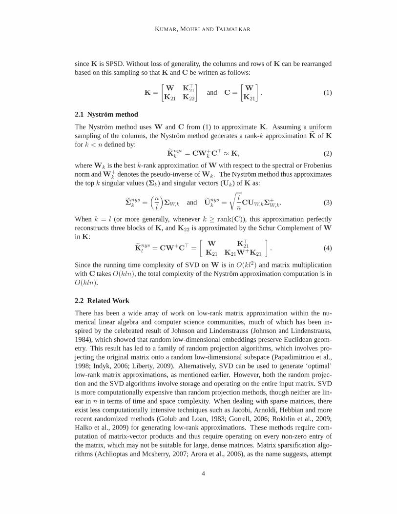
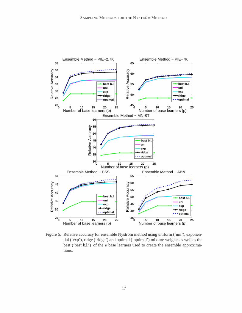
We first show results for the ensemble Nystrom method using different techniques to choosethe mixture weights, as previously discussed. In these experiments, we focused on baselearners generated via the Nystrom method with uniform sampling of columns. Further-more, for the exponential and the ridge regression variants, we sampled a set ofs = 20columns and used an additional20 columns (s′) as a hold-out set for selecting the optimalvalues ofη andλ. The number of approximations,p, was varied from2 to25. As a baseline,we also measured the maximum relative accuracy across thep Nystrom approximationsused to constructKens. We also calculated the performance when using the optimalµ, thatis, we used least-square regression to find the best possiblechoice of combination weightsfor a fixed set ofp approximations by settings= n. The results of these experiments arepresented in Figure 5.7 These results clearly show that the ensemble Nystrom performanceis significantly better than any of the individual Nystrom approximations. We further notethat the ensemble Nystrom method tends to converge very quickly, and the most significantgain in performance occurs asp increases from2 to 10.

EFFECT OF RANK

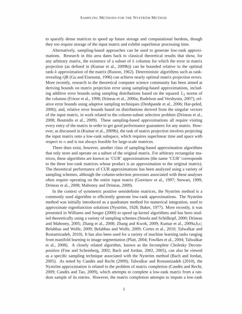
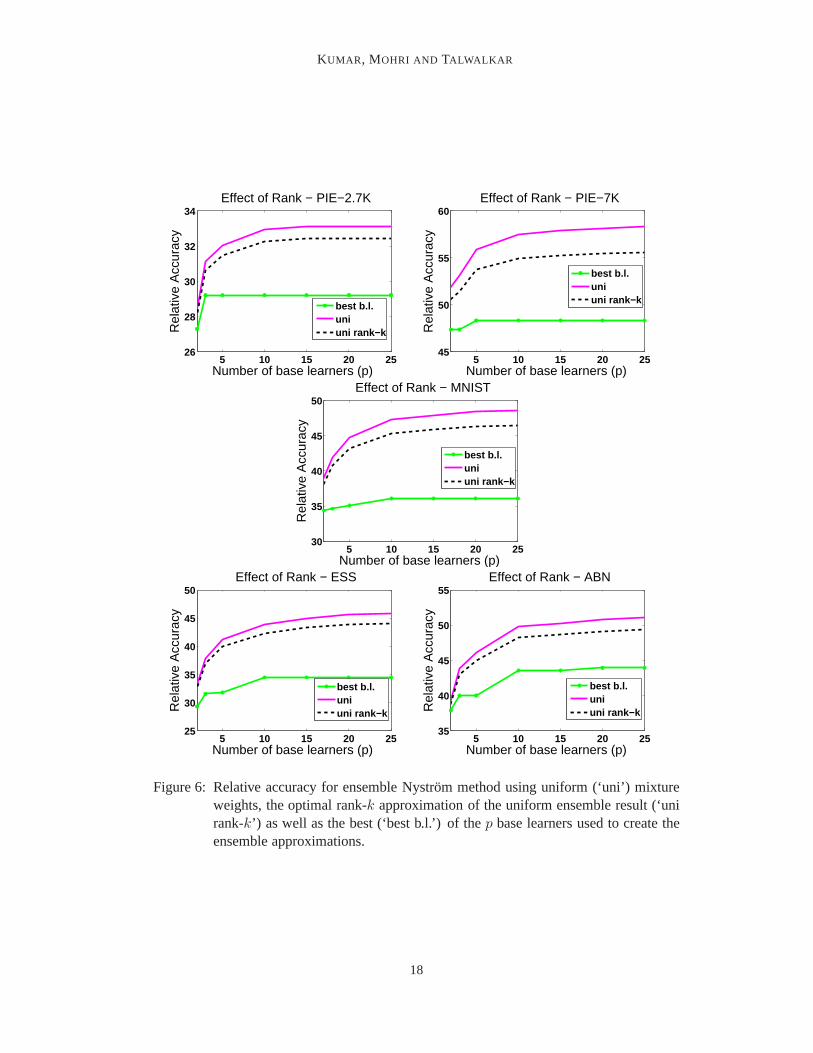
As mentioned earlier, the rank of the ensemble approximations can bep times greater thanthe rank of each of the base learners. Hence, to validate the results in Figure 5, we performeda simple experiment in which we compared the performance of the best base learner to thebest rankk approximation of the uniform ensemble approximation (obtained via SVD of theuniform ensemble approximation). We again used base learners generated via the Nystrommethod with uniform sampling of columns. The results of thisexperiment, presented inFigure 6, suggest that the performance gain of the ensemble methods is not due to thisincreased rank.

5. Note that we can also efficiently obtain singular values and singular vectors of the low-rank matrixKens

using coherence-based arguments, as in Talwalkar and Rostamizadeh (2010).6. Similar results (not reported here) were observed for other values ofk andl as well.7. Similar results (not reported here) were observed when measuring relative accuracy using the spectral norm

instead of the Frobenium norm.

16


0 5 10 15 20 2526

28

30

32

34

36

38

Number of base learners (p)

Rel

ativ

e A

ccur

acy

Ensemble Method − PIE−2.7K

best b.l.uniexpridgeoptimal

0 5 10 15 20 2545

50

55

60

65


Rel

ativ

e A

ccur

acy

Ensemble Method − PIE−7K


0 5 10 15 20 2530

35

40

45

50

55

60


Rel

ativ

e A

ccur

acy

Ensemble Method − MNIST


0 5 10 15 20 2525

30

35

40

45

50


Rel

ativ

e A

ccur

acy

Ensemble Method − ESS


0 5 10 15 20 2535

40

45

50

55

60

65


Rel

ativ

e A

ccur

acy

Ensemble Method − ABN


Figure 5: Relative accuracy for ensemble Nystrom method using uniform (‘uni’), exponen-tial (‘exp’), ridge (‘ridge’) and optimal (‘optimal’) mixture weights as well as thebest (‘best b.l.’) of thep base learners used to create the ensemble approxima-tions.

17


5 10 15 20 2526

28

30

32

34


Rel

ativ

e A

ccur

acy

Effect of Rank − PIE−2.7K

best b.l.uniuni rank−k

5 10 15 20 2545

50

55

60


Rel

ativ

e A

ccur

acy

Effect of Rank − PIE−7K


5 10 15 20 2530

35

40

45

50


Rel

ativ

e A

ccur

acy

Effect of Rank − MNIST


5 10 15 20 2525

30

35

40

45

50


Rel

ativ

e A

ccur

acy

Effect of Rank − ESS


5 10 15 20 2535

40

45

50

55


Rel

ativ

e A

ccur

acy

Effect of Rank − ABN


Figure 6: Relative accuracy for ensemble Nystrom method using uniform (‘uni’) mixtureweights, the optimal rank-k approximation of the uniform ensemble result (‘unirank-k’) as well as the best (‘best b.l.’) of thep base learners used to create theensemble approximations.

18


5 10 15 20 2532

33

34

35

36

Relative size of validation set

Rel

ativ

e A

ccur

acy

Effect of Ridge − PIE−2.7K

no−ridgeridgeoptimal

0 5 10 15 20 2555

56

57

58

59


Rel

ativ

e A

ccur

acy

Effect of Ridge − PIE−7K


5 10 15 20 2553

53.5

54

54.5

55


Rel

ativ

e A

ccur

acy

Effect of Ridge − MNIST


0 5 10 15 20 2543

43.5

44

44.5

45

45.5


Rel

ativ

e A

ccur

acy

Effect of Ridge − ESS


0 5 10 15 20 2540

45

50

55

60


Rel

ativ

e A

ccur

acy

Effect of Ridge − ABN


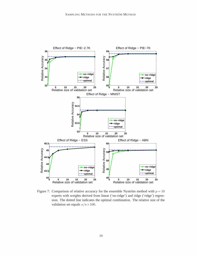
Figure 7: Comparison of relative accuracy for the ensemble Nystrom method withp= 10experts with weights derived from linear (‘no-ridge’) and ridge (‘ridge’) regres-sion. The dotted line indicates the optimal combination. The relative size of thevalidation set equalss/n×100.

19


Base Learner Method PIE-2.7K PIE-7K MNIST ESS ABNAverage Base Learner 26.9 46.3 34.2 30.0 38.1Best Base Learner 29.2 48.3 36.1 34.5 43.6

Uniform Ensemble Uniform 33.0 57.5 47.3 43.9 49.8Ensemble Exponential 33.0 57.5 47.4 43.9 49.8Ensemble Ridge 35.0 58.5 54.0 44.5 53.6Average Base Learner 47.6 62.9 62.5 42.2 60.6Best Base Learner 48.4 66.4 63.9 47.1 72.0

K-means Ensemble Uniform 54.9 71.3 76.9 52.2 76.4Ensemble Exponential 54.9 71.4 77.0 52.2 78.3Ensemble Ridge 54.9 71.6 77.2 52.7 79.0

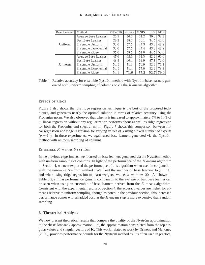
Table 4: Relative accuracy for ensemble Nystrom method with Nystrom base learners gen-erated with uniform sampling of columns or via theK-means algorithm.

EFFECT OF RIDGE

Figure 5 also shows that the ridge regression technique is the best of the proposed tech-niques, and generates nearly the optimal solution in terms of relative accuracy using theFrobenius norm. We also observed that whens is increased to approximately5% to 10% ofn, linear regression without any regularization performs about as well as ridge regressionfor both the Frobenius and spectral norm. Figure 7 shows thiscomparison between lin-ear regression and ridge regression for varying values ofs using a fixed number of experts(p = 10). In these experiments, we again used base learners generated via the Nystrommethod with uniform sampling of columns.

ENSEMBLE K-MEANS NYSTROM

In the previous experiments, we focused on base learners generated via the Nystrom methodwith uniform sampling of columns. In light of the performance of theK-means algorithmin Section 4, we next explored the performance of this algorithm when used in conjunctionwith the ensemble Nystrom method. We fixed the number of baselearners top = 10and when using ridge regression to learn weights, we sets = s′ = 20. As shown inTable 5.2, similar performance gains in comparison to the average or best base learner canbe seen when using an ensemble of base learners derived from theK-means algorithm.Consistent with the experimental results of Section 4, the accuracy values are higher forK-means relative to uniform sampling, though as noted in the previous section, this increasedperformance comes with an added cost, as theK-means step is more expensive than randomsampling.

6. Theoretical Analysis

We now present theoretical results that compare the qualityof the Nystrom approximationto the ‘best’ low-rank approximation, i.e., the approximation constructed from the top sin-gular values and singular vectors ofK. This work, related to work by Drineas and Mahoney(2005), provides performance bounds for the Nystrom method as it is often used in practice,

20


i.e., using uniform sampling without replacement, and holds for both the standard Nystrommethod as well as the ensemble Nystrom method discussed in Section 5.

Our theoretical analysis of the Nystrom method uses some results previously shownby Drineas and Mahoney (2005) as well as the following generalization of McDiarmid’sconcentration bound to sampling without replacement (Cortes et al., 2008).

Theorem 1 LetZ1, . . . , Zl be a sequence of random variables sampled uniformly withoutreplacement from a fixed set ofl+u elementsZ, and letφ : Z l→R be a symmetric functionsuch that for alli ∈ [1, l] and for all z1, . . . , zl ∈ Z and z′1, . . . , z

′l ∈ Z, |φ(z1, . . . , zl)−

φ(z1, . . . , zi−1, z′i, zi+1, . . . , zl)|≤c. Then, for allǫ>0, the following inequality holds:

Pr[φ−E[φ] ≥ ǫ

]≤ exp

[ −2ǫ2

α(l,u)c2

], (8)

whereα(l, u) = lul+u−1/2

11−1/(2 max{l,u}) .

We define theselection matrixcorresponding to a sample ofl columns as the matrixS∈R

n×l defined bySii =1 if the ith column ofK is among those sampled,Sij =0 otherwise.Thus,C=KS is the matrix formed by the columns sampled. SinceK is SPSD, there existsX ∈ R

N×n such thatK = X⊤X. We shall denote byKmax the maximum diagonal entry

of K, Kmax =maxi Kii, and bydKmax the distancemaxij

√Kii + Kjj − 2Kij .

6.1 Standard Nystrom method

The following theorem gives an upper bound on the norm-2 error of the Nystrom approxi-mation of the form‖K−K‖2/‖K‖2 ≤ ‖K−Kk‖2/‖K‖2 +O(1/

√l) and an upper bound

on the Frobenius error of the Nystrom approximation of the form ‖K − K‖F /‖K‖F ≤‖K−Kk‖F /‖K‖F +O(1/l

1

4 ).

Theorem 2 Let K denote the rank-k Nystrom approximation ofK based onl columnssampled uniformly at random without replacement fromK, andKk the best rank-k ap-proximation ofK. Then, with probability at least1− δ, the following inequalities hold forany sample of sizel:

‖K− K‖2 ≤ ‖K−Kk‖2 + 2n√lKmax

[1 +

√n−l

n−1/21

β(l,n) log 1δ d

K

max/K1

2

max

]

‖K− K‖F ≤ ‖K−Kk‖F +

[64kl

] 1

4nKmax

[1 +

√n−l

n−1/21

β(l,n) log 1δ d

K

max/K1

2

max

] 1

2

,

whereβ(l, n) = 1− 12max{l,n−l} .

Proof To bound the norm-2 error of the Nystrom method in the scenario of samplingwithout replacement, we start with the following general inequality given by Drineas andMahoney (2005)[proof of Lemma 4]:

‖K− K‖2 ≤ ‖K−Kk‖2 + 2‖XX⊤ − ZZ

⊤‖2,

whereZ=√

nl XS. We then apply the McDiarmid-type inequality of Theorem 1 toφ(S)=

‖XX⊤−ZZ

⊤‖2. Let S′ be a sampling matrix selecting the same columns asS except for

21


one, and letZ′ denote√

nl XS

′. Let z andz′ denote the only differing columns ofZ and

Z′, then

|φ(S′)− φ(S)| ≤ ‖z′z′⊤ − zz⊤‖2 = ‖(z′ − z)z′⊤ + z(z′ − z)⊤‖2

≤ 2‖z′ − z‖2 max{‖z‖2, ‖z′‖2}.

Columns ofZ are those ofX scaled by√n/l. The norm of the difference of two columns

of X can be viewed as the norm of the difference of two feature vectors associated toKand thus can be bounded bydK. Similarly, the norm of a single column ofX is bounded

by K

1

2

max. This leads to the following inequality:

|φ(S′)− φ(S)| ≤ 2n

ldKmaxK

1

2

max. (9)

The expectation ofφ can be bounded as follows:

E[Φ] = E[‖XX⊤ − ZZ

⊤‖2] ≤ E[‖XX⊤ − ZZ

⊤‖F ] ≤ n√lKmax, (10)

where the last inequality follows Corollary 2 of Kumar et al.(2009a). The inequalities(9) and (10) combined with Theorem 1 give a bound on‖XX

⊤ − ZZ⊤‖2 and yield the

statement of the theorem.The following general inequality holds for the Frobenius error of the Nystrom method

(Drineas and Mahoney, 2005):

‖K− K‖2F ≤ ‖K−Kk‖2F +√

64k ‖XX⊤ − ZZ

⊤‖2F nKmaxii . (11)

Bounding the term‖XX⊤−ZZ

⊤‖2F as in the norm-2 case and using the concentrationbound of Theorem 1 yields the result of the theorem.

6.2 Ensemble Nystrom method

The following error bounds hold for ensemble Nystrom methods based on a convex combi-nation of Nystrom approximations.

Theorem 3 LetS be a sample ofpl columns drawn uniformly at random without replace-ment fromK, decomposed intop subsamples of sizel, S1, . . . , Sp. For r ∈ [1, p], let Kr

denote the rank-k Nystrom approximation ofK based on the sampleSr, and letKk denotethe best rank-k approximation ofK. Then, with probability at least1 − δ, the followinginequalities hold for any sampleS of sizepl and for anyµ in the unit simplex∆ andK

ens =∑p

r=1 µrKr:

‖K− Kens‖2 ≤ ‖K−Kk‖2 +

2n√lKmax

[1 + µmaxp

1

2

√n−pl

n−1/21

β(pl,n) log 1δ d

K

max/K1

2

max

]

‖K− Kens‖F ≤ ‖K−Kk‖F +

[64kl

] 1

4nKmax

[1 + µmaxp

1

2

√n−pl

n−1/21

β(pl,n) log 1δ d

K

max/K1

2

max

] 1

2

,

whereβ(pl, n) = 1− 12max{pl,n−pl} andµmax = maxp

r=1 µr.

22


Proof For r ∈ [1, p], let Zr =√n/lXSr, whereSr denotes the selection matrix cor-

responding to the sampleSr. By definition ofKens and the upper bound on‖K − Kr‖2already used in the proof of theorem 2, the following holds:

‖K− Kens‖2 =

∥∥∥p∑

r=1

µr(K− Kr)∥∥∥

2≤

p∑

r=1

µr‖K− Kr‖2

≤p∑

r=1

µr

(‖K−Kk‖2 + 2‖XX

⊤ − ZrZ⊤r ‖2

)

= ‖K−Kk‖2 + 2

p∑

r=1

µr‖XX⊤ − ZrZ

⊤r ‖2.

We apply Theorem 1 toφ(S) =∑p

r=1 µr‖XX⊤ − ZrZ

⊤r ‖2. Let S′ be a sample differing

from S by only one column. Observe that changing one column of the full sampleSchanges only one subsampleSr and thus only one termµr‖XX

⊤ − ZrZ⊤r ‖2. Thus, in

view of the bound (9) on the change to‖XX⊤ − ZrZ

⊤r ‖2, the following holds:

|φ(S′)− φ(S)| ≤ 2n

lµmaxd

K

maxK

1

2

max, (12)

The expectation ofΦ can be straightforwardly bounded by:

E[Φ(S)] =

p∑

r=1

µr E[‖XX⊤ − ZrZ

⊤r ‖2] ≤

p∑

r=1

µrn√lKmax =

n√lKmax

using the bound (10) for a single expert. Plugging in this upper bound and the Lipschitzbound (12) in Theorem 1 yields the norm-2 bound for the ensemble Nystrom method.

For the Frobenius error bound, using the convexity of the Frobenius norm square‖·‖2Fand the general inequality (11), we can write

‖K− Kens‖2F =

∥∥∥p∑

r=1

µr(K− Kr)∥∥∥

2

F≤

p∑

r=1

µr‖K− Kr‖2F

≤p∑

r=1

µr

[‖K−Kk‖2F +

√64k ‖XX

⊤ − ZrZ⊤r ‖F nKmax

ii

].

= ‖K−Kk‖2F +√

64k

p∑

r=1

µr‖XX⊤ − ZrZ

⊤r ‖F nKmax

ii .

The result follows by the application of Theorem 1 toψ(S)=∑p

r=1 µr‖XX⊤ − ZrZ

⊤r ‖F

in a way similar to the norm-2 case.

The bounds of Theorem 3 are similar in form to those of Theorem2. However, thebounds for the ensemble Nystrom are tighter than those for any Nystrom expert based ona single sample of sizel even for a uniform weighting. In particular, forµi = 1/p forall i, the last term of the ensemble bound for norm-2 is smaller by afactor larger thanµmaxp

1

2 = 1/√p.

23


7. Conclusion

A key aspect of sampling-based matrix approximations is themethod for the selection ofrepresentative columns. We discussed both fixed and adaptive methods for sampling thecolumns of a matrix. We saw that the approximation performance is significantly affectedby the choice of the sampling algorithm and also that there isa tradeoff between choosinga more informative set of columns and the efficiency of the sampling algorithm. Further-more, we introduced and discussed a new meta-algorithm based on an ensemble of severalmatrix approximations that generates favorable matrix reconstructions using base learnersderived from either fixed or adaptive sampling schemes, and naturally fits within a dis-tributed computing environment, thus making it quite efficient even in large-scale settings.We concluded with a theoretical analysis of the Nystrom method (both the standard ap-proach and the ensemble method) as it is often used in practice, namely using uniformsampling without replacement.

Acknowledgments

AT was supported by NSF award No.1122732. We thank the editor and the reviewers forseveral insightful comments that helped improve the original version of this paper.

References

Dimitris Achlioptas and Frank Mcsherry. Fast computation of low-rank matrix approxima-tions. Journal of the ACM, 54(2), 2007.

Sanjeev Arora, Elad Hazan, and Satyen Kale. A fast random sampling algorithm for spar-sifying matrices. InApprox-Random, 2006.

A. Asuncion and D.J. Newman. UCI machine learning repository.http://www.ics.uci.edu/ mlearn/MLRepository.html, 2007.

Francis R. Bach and Michael I. Jordan. Kernel Independent Component Analysis.Journalof Machine Learning Research, 3:1–48, 2002.

Francis R. Bach and Michael I. Jordan. Predictive low-rank decomposition for kernel meth-ods. InInternational Conference on Machine Learning, 2005.

Christopher T. Baker.The numerical treatment of integral equations. Clarendon Press,Oxford, 1977.

M. A. Belabbas and P. J. Wolfe. Spectral methods in machine learning and new strategiesfor very large datasets.Proceedings of the National Academy of Sciences of the UnitedStates of America, 106(2):369–374, January 2009. ISSN 1091-6490.

M.-A. Belabbas and P. J. Wolfe. On landmark selection and sampling in high-dimensionaldata analysis.arXiv:0906.4582v1 [stat.ML], 2009.

Bernhard E. Boser, Isabelle Guyon, and Vladimir N. Vapnik. Atraining algorithm foroptimal margin classifiers. InConference on Learning Theory, 1992.

24


Christos Boutsidis, Michael W. Mahoney, and Petros Drineas. An improved approximationalgorithm for the column subset selection problem. InSymposium on Discrete Algo-rithms, 2009.

Roland Bunschoten.http://www.mathworks.com/matlabcentral/fileexchange/71-distance-m/, 1999.

Emmanuel J. Candes and Benjamin Recht. Exact matrix completion via convex optimiza-tion. Foundations of Computational Mathematics, 9(6):717–772, 2009.

Emmanuel J. Candes and Terence Tao. The power of convex relaxation: Near-optimalmatrix completion.arXiv:0903.1476v1 [cs.IT], 2009.

Gavin Cawley and Nicola Talbot. Miscellaneous MATLAB software.http://theoval.cmp.uea.ac.uk/matlab/default.html#cholinc,2004.

Corinna Cortes and Vladimir N. Vapnik. Support-Vector Networks. Machine Learning, 20(3):273–297, 1995.

Corinna Cortes, Mehryar Mohri, Dmitry Pechyony, and AshishRastogi. Stability of trans-ductive regression algorithms. InInternational Conference on Machine Learning, 2008.

Corinna Cortes, Mehryar Mohri, and Ameet Talwalkar. On the impact of kernel approxima-tion on learning accuracy. InConference on Artificial Intelligence and Statistics, 2010.

Vin de Silva and Joshua Tenenbaum. Global versus local methods in nonlinear dimension-ality reduction. InNeural Information Processing Systems, 2003.

Amit Deshpande, Luis Rademacher, Santosh Vempala, and Grant Wang. Matrix approxi-mation and projective clustering via volume sampling. InSymposium on Discrete Algo-rithms, 2006.

Petros Drineas. Personal communication, 2008.

Petros Drineas and Michael W. Mahoney. On the Nystrom method for approximating aGram matrix for improved kernel-based learning.Journal of Machine Learning Re-search, 6:2153–2175, 2005.

Petros Drineas, Eleni Drinea, and Patrick S. Huggins. An experimental evaluation of aMonte-Carlo algorithm for SVD. InPanhellenic Conference on Informatics, 2001.

Petros Drineas, Ravi Kannan, and Michael W. Mahoney. Fast Monte Carlo algorithmsfor matrices II: Computing a low-rank approximation to a matrix. SIAM Journal ofComputing, 36(1), 2006a.

Petros Drineas, Ravi Kannan, and Michael W. Mahoney. Fast Monte Carlo algorithmsfor matrices II: Computing a low-rank approximation to a matrix. SIAM Journal onComputing, 36(1), 2006b.

25


Petros Drineas, Michael W. Mahoney, and S. Muthukrishnan. Relative-error CUR matrixdecompositions.SIAM Journal on Matrix Analysis and Applications, 30(2):844–881,2008.

Shai Fine and Katya Scheinberg. Efficient SVM training usinglow-rank kernel representa-tions. Journal of Machine Learning Research, 2:243–264, 2002.

Charless Fowlkes, Serge Belongie, Fan Chung, and Jitendra Malik. Spectral grouping usingthe Nystrom method.Transactions on Pattern Analysis and Machine Intelligence, 26(2):214–225, 2004.

Alan Frieze, Ravi Kannan, and Santosh Vempala. Fast Monte-Carlo algorithms for findinglow-rank approximations. InFoundation of Computer Science, 1998.

Gene Golub and Charles Van Loan.Matrix Computations. Johns Hopkins University Press,Baltimore, 2nd edition, 1983. ISBN 0-8018-3772-3 (hardcover), 0-8018-3739-1 (paper-back).

S. A. Goreinov, E. E. Tyrtyshnikov, and N. L. Zamarashkin. A theory of pseudoskeletonapproximations.Linear Algebra and Its Applications, 261:1–21, 1997.

G. Gorrell. Generalized Hebbian algorithm for incrementalSingular Value Decompositionin natural language processing. InEuropean Chapter of the Association for Computa-tional Linguistics, 2006.

Ming Gu and Stanley C. Eisenstat. Efficient algorithms for computing a strong rank-revealing QR factorization.SIAM Journal of Scientific Computing, 17(4):848–869, 1996.

A. Gustafson, E. Snitkin, S. Parker, C. DeLisi, and S. Kasif.Towards the identifica-tion of essential genes using targeted genome sequencing and comparative analysis.BMC:Genomics, 7:265, 2006.

Nathan Halko, Per Gunnar Martinsson, and Joel A. Tropp. Finding structure with ran-domness: Stochastic algorithms for constructing approximate matrix decompositions.arXiv:0909.4061v1 [math.NA], 2009.

Sariel Har-peled. Low-rank matrix approximation in lineartime, manuscript, 2006.

Piotr Indyk. Stable distributions, pseudorandom generators, embeddings, and data streamcomputation.Journal of the ACM, 53(3):307–323, 2006.

W. B. Johnson and J. Lindenstrauss. Extensions of Lipschitzmappings into a Hilbert space.Contemporary Mathematics, 26:189–206, 1984.

Sanjiv Kumar, Mehryar Mohri, and Ameet Talwalkar. Samplingtechniques for the Nystrommethod. InConference on Artificial Intelligence and Statistics, 2009a.

Sanjiv Kumar, Mehryar Mohri, and Ameet Talwalkar. On sampling-based approximatespectral decomposition. InInternational Conference on Machine Learning, 2009b.

26


Sanjiv Kumar, Mehryar Mohri, and Ameet Talwalkar. EnsembleNystrom method. InNeural Information Processing Systems, 2009c.

Yann LeCun and Corinna Cortes. The MNIST database of handwritten digits.http://yann.lecun.com/exdb/mnist/, 1998.

Mu Li, James T. Kwok, and Bao-Liang Lu. Making large-scale Nystrom approximationpossible. InInternational Conference on Machine Learning, 2010.

Edo Liberty.Accelerated dense random projections. Ph.D. thesis, computer science depart-ment, Yale University, New Haven, CT, 2009.

N. Littlestone and M. K. Warmuth. The Weighted Majority algorithm. Information andComputation, 108(2):212–261, 1994.

Rong Liu, Varun Jain, and Hao Zhang. Subsampling for efficient spectral mesh processing.In Computer Graphics International Conference, 2006.

Michael W Mahoney and Petros Drineas. CUR matrix decompositions for improved dataanalysis.Proceedings of the National Academy of Sciences, 106(3):697–702, 2009.

E.J. Nystrom. Uber die praktische auflosung von linearen integralgleichungen mit an-wendungen auf randwertaufgaben der potentialtheorie.Commentationes Physico-Mathematicae, 4(15):1–52, 1928.

M. Ouimet and Y. Bengio. Greedy spectral embedding. InArtificial Intelligence and Statis-tics, 2005.

Christos H. Papadimitriou, Hisao Tamaki, Prabhakar Raghavan, and Santosh Vempala. La-tent Semantic Indexing: a probabilistic analysis. InPrinciples of Database Systems,1998.

John C. Platt. Fast embedding of sparse similarity graphs. In Neural Information ProcessingSystems, 2004.

Vladimir Rokhlin, Arthur Szlam, and Mark Tygert. A randomized algorithm for PrincipalComponent Analysis.SIAM Journal on Matrix Analysis and Applications, 31(3):1100–1124, 2009.

Mark Rudelson and Roman Vershynin. Sampling from large matrices: An approach throughgeometric functional analysis.Journal of the ACM, 54(4):21, 2007.

A. F. Ruston. Auerbach’s theorem and tensor products of Banach spaces.MathematicalProceedings of the Cambridge Philosophical Society, 58:476–480, 1962.

Bernhard Scholkopf and Alex Smola.Learning with Kernels. MIT Press: Cambridge, MA,2002.

Bernhard Scholkopf, Alexander Smola, and Klaus-Robert M¨uller. Nonlinear componentanalysis as a kernel eigenvalue problem.Neural Computation, 10(5):1299–1319, 1998.

27


Terence Sim, Simon Baker, and Maan Bsat. The CMU pose, illumination, and expressiondatabase. InConference on Automatic Face and Gesture Recognition, 2002.

Alex J. Smola. SVLab.http://alex.smola.org/data/svlab.tgz, 2000.

Alex J. Smola and Bernhard Scholkopf. Sparse Greedy MatrixApproximation for machinelearning. InInternational Conference on Machine Learning, 2000.

G. W. Stewart. Four algorithms for the efficient computationof truncated pivoted QR ap-proximations to a sparse matrix.Numerische Mathematik, 83(2):313–323, 1999.

Ameet Talwalkar and Afshin Rostamizadeh. Matrix coherenceand the Nystrom method.In Conference on Uncertainty in Artificial Intelligence, 2010.

Ameet Talwalkar, Sanjiv Kumar, and Henry Rowley. Large-scale manifold learning. InConference on Vision and Pattern Recognition, 2008.

Mark Tygert.http://www.mathworks.com/matlabcentral/fileexchange/21524-principal-component-analysis, 2009.

Christopher K. I. Williams and Matthias Seeger. Using the Nystrom method to speed upkernel machines. InNeural Information Processing Systems, 2000.

Kai Zhang and James T. Kwok. Density-weighted Nystrom method for computing largekernel eigensystems.Neural Computation, 21(1):121–146, 2009.

Kai Zhang, Ivor Tsang, and James Kwok. Improved Nystrom low-rank approximation anderror analysis. InInternational Conference on Machine Learning, 2008.

28

Documents

Sampling Methods for the Nystrom Method¨