Local Variance Gamma and Explicit Calibration toOption Prices ∗†‡

Peter CarrNew York University

Sergey NadtochiyUniversity of Michigan

Abstract

In some options markets (e.g. commodities), options are listed with only a singlematurity for each underlying. In others, (e.g. equities, currencies), options are listedwith multiple maturities. In this paper, we analyze a special class of pure jump Markovmartingale models and provide an algorithm for calibrating such models to match themarket prices of European options with multiple strikes and maturities. This algorithmmatches option prices exactly and only requires solving several one-dimensional root-search problems and applying elementary functions. We show how to construct a time-homogeneous process which meets a single smile, and a piecewise time-homogeneousprocess which can meet multiple smiles.

1 Introduction

Why is there always so much month left at the end of the money? – Sarah Lloyd

The very earliest literature on option pricing imposed a process on the underlying assetprice and derived unique option prices as a consequence of the dynamical assumptions and noarbitrage. We may characterize this literature as going “From Process to Prices”. However,once the notion of implied volatility was introduced, the inverse problem of going “FromPrices to Process” was established. The term that practitioners favor for this inverse problemis calibration - the practice of determining the required inputs to a model so that they areconsistent with a specified set of market prices. Implied volatility is just the simplest example

∗This version: July 23, 2014. First version April 11, 2012.†We are very grateful for comments from Laurent Cousot, Bruno Dupire, David Eliezer, Travis Fisher,

Bjorn Flesaker, Alexey Polishchuk, Serge Tchikanda, Arun Verma, Jan Ob loj, and Liuren Wu. We also thankthe anonymous referee for valuable remarks and suggestions which helped us improve the paper significantly.We are responsible for any remaining errors.‡Address correspondence to Sergey Nadtochiy, Mathematics Department, University of Michigan, 530

Church Street, Ann Arbor, MI 48109, USA; e-mail: sergeyn@umich.edu.

1

of this calibration procedure, wherein a single option price is given and the volatility input tothe Black Scholes model is determined so as to gain exact consistency with this one marketprice.

When the number of calibration instruments is expanded to several options of differentmaturities, the Black Scholes model can be readily adapted to be consistent with this in-formation set. One simply assumes that the instantaneous variance is a piecewise constantfunction of time, which jumps at each option maturity. The staircase levels are chosen sothat the time-averaged cumulative variance matches the implied variance at each maturity.So long as the given option prices are arbitrage-free, this deterministic volatility versionof the Black Scholes model is capable of achieving exact consistency with any given termstructure of market option prices. As a bonus, the ability to have closed form solutions forEuropean option prices is retained.

Unfortunately, when the number of calibration instruments is instead expanded to severalco-terminal options of different strikes, there is no unique simple extension of the BlackScholes model which is capable of meeting this information set. Whenever the impliedvolatility at a single term is a non-constant function of the strike price, there are, instead,many ways to gain exact consistency with the associated option prices. The earliest workon this problem seems to be [Rubinstein and Rubinstein, 1994] in his presidential address.Working in a discrete time setting, he assumed that the price of the underlying asset isa Markov chain evolving on a binomial lattice. Assuming that the terminal nodes of thelattice fell on option strikes, he was able to find the nodes and the transition probabilitiesthat determine this lattice. A continuous time and state version of the Rubinstein resultcan be found in [Carr and Madan, 1998]. Other methods of calibrating to a single smile arepresented in [Cox et al., 2011], [Ekstrom et al., 2013], [Noble, 2013], and to multiple smiles,in [Madan and Yor, 2002]. However, all these works assume the availability of continuoussmiles, i.e. option prices for a continuum of strikes.

In this paper, we present a new way to go from a given set of option prices to a Markovianmartingale in a continuous time setting. This calibration method can be successfully appliedto continuous smiles, as well as a finite family of option prices with multiple strikes and matu-rities. In order to implement our algorithm, one only needs to solve several one-dimensionalroot-search problems and apply the elementary functions. To the authors’ knowledge, thisis the first example of explicit exact calibration to a finite set of option prices with multiplestrikes and maturities, such that the calibrated (continuous time) process has continuous dis-tribution at all times. In addition, if the given market options are co-terminal, the calibratedprocess becomes time-homogeneous.

Suppose that the risk-neutral process for the (forward) price of an asset, underlying a setof European options, is a driftless time-homogeneous diffusion running on an independentand unbiased Gamma process. We christen this model “Local Variance Gamma” (LVG),because it combines ideas from both the Local Variance model of [Dupire, 1994] and theVariance Gamma model of [Madan and Seneta, 1990]. As the diffusion is time-homogeneousand the subordinating Gamma process is Levy, their independence implies that the spot priceprocess is also Markov and time-homogeneous. As the subordinator is a pure jump process,the LVG process governing the underlying spot price is also pure jump. In addition, theforward and backward equations governing options prices in the LVG model turn into muchsimpler partial differential difference equations (PDDEs). The existence of these PDDEs

2

permits both explicit calibration of the LVG model and fast numerical valuation of contingentclaims. As a result of the forward PDDE holding, the diffusion coefficient can be explicitlyrepresented (calibrated) in terms of a single (continuous) smile. The backward PDDE,then, allows for efficient valuation of other contingent claims, by successively solving a finitesequence of second order linear ordinary differential equations (ODEs) in the spatial variable.

While the single smile results are relevant for commodity option markets, they are notas relevant for market makers in equity and currency options markets where multiple optionmaturities trade simultaneously. In order to be consistent with multiple smiles, we alsopresent an extension of the LVG model that results in a piecewise time-homogeneous processfor the underlying asset price. The calibration procedure remains explicit in the case ofmultiple smiles: in particular, it does not require application of any optimization methods.

The above results allow us to calibrate the LVG model, or its extension, to continuousarbitrage-free smiles, implying, in particular, that option prices for a continuum of strikesmust be observed in the market. To get rid of this unrealistic assumption, we show how to usethe PDDEs associated with the LVG model to construct continuous arbitrage-free smiles froma finite family of option prices, for multiple strikes and maturities. To the authors’ knowledge,this is the first construction of a continuously differentiable arbitrage-free interpolation ofimplied volatility across strikes, that only requires solutions to one-dimensional root-searchproblems and application of elementary functions.

This paper is structured as follows. In the next section, we present the basic assumptionsand construct the LVG process, i.e. a driftless time-homogeneous diffusion subordinated toan unbiased gamma process. In the following section, we derive the forward and backwardPDDEs that govern option prices. In the penultimate section, we discuss calibration strate-gies. To meet multiple smiles, we construct a piecewise time-homogeneous extension of theLVG process and develop the corresponding forward and backward PDDEs. The algorithmfor constructing continuous smiles from a finite set of option prices, along with the corre-sponding theorem and numerical results, is presented in Subsection 4.3. The final sectionsummarizes the paper and makes some suggestions for future research.

2 Local Variance Gamma Process

2.1 Model Assumptions

In this subsection, we lay out the general financial and mathematical assumptions usedthroughout the paper. For simplicity, we assume zero carrying costs for all assets. As aresult, we have zero interest rates, dividend yields, etc. It is straightforward to extend ourresults to the case where these quantities are deterministic functions of time (the associatednumerical issues are discussed in Remark 19). We also assume frictionless markets and noarbitrage. Motivated by the fundamental theorem of asset pricing, we assume that thereexists a probability measure Q such that market prices of all assets are Q-martingales.Following standard terminology, we will refer to Q as a risk-neutral probability measure.

We assume that the market includes a family of European call options written on acommon underlying asset whose prices process we denote by S. We assume that the initialspot price S0 is known. Throughout this paper, we denote by (L,U), with −∞ ≤ L < U ≤

3

∞, the spatial interval on which the S process lives. The boundary points L and U mayor may not be attainable. If a boundary point is attainable, we assume that the process isabsorbed at that point. If a boundary point is infinite, we assume it is not attainable. Aswe interpret S as the price process, for simplicity, one can think of L and U as 0 and ∞,respectively.

In the following subsections, we consider several specific classes of the underlying pro-cesses and use them as building blocks to construct the Local Variance Gamma process.Namely, the desired pure-jump process arises by subordinating a driftless diffusion to anunbiased gamma process.

2.2 Driftless Diffusion

To elaborate on this additional structure, let W be a standard Brownian motion. We defineD as a driftless time-homogeneous diffusion with the generator 1

2a2(D)∂2

DD,

dDs = a(Ds)dWs, s ∈ [0, ζ], (1)

and with the initial value x ∈ (L,U). The stopping time ζ denotes the first time thediffusion exits the interval (L,U). The process is stopped (absorbed) at ζ. We assumethat the diffusion coefficient a : (L,U) → (0,∞) is a piecewise continuous function, witha finite number of discontinuities of the first order (i.e. the left and right limits exist ateach point), bounded uniformly from above and away from zero, and having finite limits atthose boundary points that are finite. Under these assumptions, for any initial conditionx ∈ (L,U), the SDE (1) has a weak solution which is unique in the sense of probability law(cf. Theorem 5.7, on p. 335, in [Karatzas and Shreve, 1998]). It is easy to see that, underthese assumptions, a boundary point, L or U , is accessible if and only if it is finite. Notealso that one can extend the set of initial conditions to the entire real line by assuming thatthe solution to (1) remains at x, for any x ∈ R \ (L,U). The collection of distributions ofthe weak solutions to (1), for all x ∈ R, forms a Markov family, in the sense of Definition2.5.11, on p. 74, in [Karatzas and Shreve, 1998]. More precisely, on the canonical space ofcontinuous paths ΩD = C ([0,∞)), equipped with the Borel sigma algebra B (C ([0,∞))),we consider a family of probability measures

QD,x

, for x ∈ R, such that every QD,x is

the distribution of a weak solution to (1), with initial condition x. As follows, for example,from Theorem 5.4.20 and Remark 5.4.21, on p. 322, in [Karatzas and Shreve, 1998],

QD,x

and the canonical process D : ω 7→ (ω(t), t ≥ 0) form a Markov family. Due to the growthrestrictions on a, D is a true martingale, with respect to its natural filtration, under anymeasure QD,x.

It is worth mentioning that there is a reason why we construct D in this particularway, introducing the family

QD,x

. Namely, in order to carry out the constructions in

Subsections 2.4 and, in turn, 4.2, we need to consider the diffusion process D as a functionof its initial condition x. In particular, we use certain properties of its distribution QD,x,such as the measurability of the mapping x 7→ QD,x, which follows from the definition of aMarkov family (cf. Definition 2.5.11, on p. 74, in [Karatzas and Shreve, 1998]).

We can compute prices of European options in a model where the risk-neutral dynamicsof the underlying are given by the above driftless diffusion. Namely, given a Borel measurable

4

and exponentially bounded payoff function φ, we recall the time t price of the associatedEuropean type claim, with the time of maturity T :

V D,φt (T ) = Ex

(φ(DT )| FDt

)= Ey (φ(DT−t))|y=Dt

,

which holds for all x ∈ R and t ∈ [0, T ]. In the above, we denote by Ex the expectation withrespect to QD,x and by FD the filtration generated by D. The last equality is due to theMarkov property. Thus, in a driftless diffusion model, the price of a European type option,at any time, can be computed via the price function:

V D,φ(τ, x) = Ex (φ(Dτ )) . (2)

Throughout the paper, τ is used as an auxiliary variables, which, often, has a meaning ofthe time to maturity : τ = T − t. In addition, we differentiate prices, as random variables,from the price functions by adding a subscript (typically, “t”). The option price function ina driftless diffusion model is expected to satisfy the Black-Scholes equation in (τ, x):

∂τVD,φ(τ, x) =

1

2a2(x)∂2

xxVD,φ(τ, x), V D,φ(0, x) = φ(x). (3)

Notice, however, that the coefficient in the above equation can be discontinuous, therefore,we can only expect the value function to satisfy this equation in a weak sense.

Theorem 1. Assume that φ : (L,U)→ R is exponentially bounded and continuously differ-entiable, and that φ′ is absolutely continuous, with a square integrable derivative. Then, V D,φ

(defined in (2)) is the unique weak solution to (3), in the sense that: V D,φ is continuous, itsweak derivatives ∂τV

D,φ and ∂2xxV

D,φ are square integrable in (0, T ) × (L,U), for any fixedT > 0, and V D,φ satisfies (3).

The proof of Theorem 1 is given in Appendix A. For a special class of contingent claims,we can derive an additional parabolic PDE, satisfied by the option prices. Recall that, in adriftless diffusion model, the price of a call option with strike K and maturity T is given by:

CDt (T,K) = Ex

((DT −K)+

∣∣FDt ) = CD(T − t,K,Dt),

for all x ∈ R and t ∈ [0, T ]. In the above, we denote by CD the call price function, which isdefined as

CD(τ,K, x) = Ex((Dτ −K)+

). (4)

The call price function satisfies another parabolic PDE, in (τ,K), known as the Dupire’sequation:

∂τCD(τ,K, x) =

1

2a2(K)∂2

KKCD(τ,K, x). (5)

Due to the possible discontinuity of a, we can only establish this equation in a weak sense.

Theorem 2. For any x ∈ (L,U), the call price function CD(τ,K, x) (defined in (4)) isabsolutely continuous as a function of K ∈ [L,U ]. Its partial derivative ∂KC

D(τ, . , x) has aunique nondecreasing and right continuous modification, which defines a probability measure

5

on [L,U ] (choosing ∂KCD(τ, U, x) = 0). Moreover, for any bounded Borel function φ, with

a compact support in (L,U), we have∫ U

L

CD(τ,K, x)φ(K)dK =

∫ U

L

(x−K)+φ(K)dK+1

2

∫ τ

0

∫ U

L

a2(K)φ(K) d(∂KC

D(u,K, S))du,

(6)for all τ > 0 and all x ∈ (L,U).

The proof of Theorem 2 is given in Appendix A.

2.3 Gamma Process

Let Γt(t∗, α), t > 0 be an independent gamma process with parameters t∗ > 0 and α > 0.As is well known, a gamma process is an increasing Levy process whose Levy density is givenby:

kΓ(t) =e−αt

t∗t, t > 0, (7)

with parameters t∗ > 0 and α > 0. Intuitively, jumps whose sizes lie in the interval [t, t+ dt]are generated by a Poisson process with intensity kΓ(t)dt. The fraction 1/t∗ controls the rateof jump arrivals, while 1/α controls the mean jump size, given that a jump has occurred.One can also get direct intuition on t∗ and α, rather than their reciprocals. As a gammaprocess has infinite activity, the number of jumps over any finite time interval is infinite forsmall jumps and finite for large jumps. If we ignore the small jumps, then the larger is t∗, thelonger one must wait on average for a fixed number of large jumps to occur. Furthermore,the larger is α, the longer it takes the running sum of these large jumps to reach a fixedpositive level. For an introduction to gamma processes, and Levy processes more generally,see [Bertoin, 1996], [Sato, 1999], or [Applebaum, 2004]. For their application in a financialcontext, see [Schoutens, 2003] or [Cont and Tankov, 2004].

The marginal distribution of a gamma process at time t ≥ 0 is a gamma distribution:

QΓt ∈ ds =αt/t

∗

Γ(t/t∗)st/t

∗−1e−αsds, s > 0, t > 0, (8)

for parameters α > 0 and t∗ > 0. For t < t∗, this PDF has a singularity at s = 0, while fort > t∗, the PDF vanishes at s = 0. At t = t∗, the PDF is exponential with mean 1

α. As a

result, we henceforth refer to the parameter t∗ > 0 as the characteristic time of the Gammaprocess. The characteristic time t∗ of a Gamma process Γ is the unique deterministic waitingtime t until the distribution of Γt is exponential.

Recall that the mean of Γt is given by:

EQΓt =t

αt∗, (9)

for all t ≥ 0. If we set the parameter α = 1/t∗, then the gamma process becomes unbiased,i.e. EQΓt = t for all t ≥ 0. In general, the variance of Γt is:

t

α2t∗, t > 0. (10)

6

As a result, the standard deviation of an unbiased gamma process Γt is just the geometricmean of t and t∗. Setting α = 1/t∗ in (10), we obtain the unbiased Gamma process. Thedistribution of the unbiased gamma process Γ at time t ≥ 0 is:

QΓt ∈ ds =st/t

∗−1e−s/t∗

(t∗)t/t∗Γ(t/t∗)ds, s > 0, (11)

When t = t∗, this PDF is exponential, and the fact that the gamma process is unbiasedimplies that the mean and the standard deviation of Γt∗ are both t∗.

Remark 3. The choice of α = 1/t∗ in the above construction is motivated merely by thedesire to have a Gamma process which is unbiased: its expectation at time t is equal to t.We consider this as a natural property, because, in what follows, we use the Gamma processas a time change. However, it is not at all necessary for the Gamma process to be unbiased.In fact, the results of the subsequent sections will hold for any α > 0. In particular, if theunbiased Gamma process produces unrealistic paths (e.g. having a lot of very small jumpsand very few extremely large ones), one may change the parameter α to obtain more realisticdynamics.1

2.4 Construction of the Local Variance Gamma Process

We assume that the risk-neutral process of the underlying spot price S is obtained by subor-dinating the driftless diffusion D to an independent unbiased gamma process Γ. Recall thatD is constructed as the canonical process on the space of continuous paths ΩD = C ([0,∞)),equipped with the Borel sigma algebra B (C ([0,∞))), and with the probability measuresQD,x, for x ∈ R. On a different probability space

(ΩΓ,FΓ

), with a probability measure QΓ,

we construct an unbiased gamma process Γ, with parameter t∗. Finally, on the product space(ΩD × ΩΓ,B (C ([0,∞)))⊗FΓ

)we define the risk-neutral dynamics of the underlying, for

every (ω1, ω2) ∈ ΩD × ΩΓ, as follows:

St(ω1, ω2) = DΓt(ω2)(ω1), t ≥ 0. (12)

It can be shown easily, by conditioning, that S inherits the martingale property of D, withrespect to its natural filtration, under any measure

Qx = QD,x ×QΓ. (13)

Remark 4. Considered as a function of the forward spatial variable, the PDF of St (when itexists) may possess some unusual properties for t small but not infinitesimal. For example,when a is constant, it is easy to see that the PDF is infinite at x, for times t < t∗/2. Asa result, for short term options, the graph of value against strike will be C1, but not C2.Similarly, gamma will not exist for short term ATM options. For a piecewise continuous a,we conjecture that the PDF of St has a jump at every point of discontinuity of a. Then, atevery such point, the call price is C1, but not C2, viewed as a function of strike.

1We thank Jan Ob loj for pointing out that the simulated paths of the unbiased Gamma process may lookunrealistic, for certain values of t∗

7

As a diffusion time changed with an independent Levy clock, the process S, along withQx (defined in (13)), for x ∈ R, form a Markov family. The following proposition makesthis statement rigorous and, in addition, shows how to reduce the computation of optionprices in the LVG model to the case of driftless diffusion. Recall that, in a model where therisk-neutral dynamics of underlying are given by S, with initial value S0 = x, the time tprice of a European type option with payoff function φ and maturity T is given by

V φt (T ) = Ex

(φ(ST )| FSt

), (14)

where FS is the filtration generated by S, and, with a slight abuse of notation, we denoteby Ex the expectation with respect to Qx. The following proposition, in particular, showsthat option prices in a LVG model are determined by the price function, defined as

V φ(τ, x) = Exφ(Sτ ), (15)

Proposition 5. The process S and the family of measures Qxx∈R form a Markov family(cf. Definition 2.5.11 in [Karatzas and Shreve, 1998]). In particular, for any Borel measur-able and exponentially bounded function φ, the following holds, for all T ≥ 0 and x ∈ R:

V φt (T ) = V φ(T − t, St), V φ(τ, x) =

∫ ∞0

uτ/t∗−1e−u/t

∗

(t∗)τ/t∗Γ(τ/t∗)V D,φ(u, x)du, (16)

where V φt , V φ, and V D,φ are given by (14), (15), and (2), respectively.

Proof. According to Definition 2.5.11 and Proposition 2.5.13 in [Karatzas and Shreve, 1998],in order to prove that S and Qxx∈R form a Markov family, we need to show two properties.First, for any F ∈ B (C ([0,∞))) ⊗ FΓ, the mapping x 7→ Qx(F ) =

(QD,x ×QΓ

)(F ) is

universally measurable. This property can be deduced easily from the universal measurabilityof the mapping x 7→ QD,x(F ), for any F ∈ B (C ([0,∞))), via the monotone class theorem.Secondly, we need to verify that, for any B ∈ B(R) and any u, t ≥ 0,

Qx(Su+t ∈ B| FSu

)= Qy (St ∈ B)|y=Su

.

The latter is done easily by conditioning on Γ and using the Markov property of D. Similarly,one obtains the second equation in (16). The first equation in (16) follows from the Markovproperty.

Suppose that time to maturity τ is equal to the characteristic time t∗ of the gammaprocess. Then (16) yields

V φ(t∗, x) =

∫ ∞0

e−u/t∗

t∗V D,φ(u, x)du. (17)

In particular, for the call options, we obtain:

Ct(T,K) = Ex(

(ST −K)+∣∣FSt ) = C(T − t,K, St),

where C(τ,K, x) is the call price function in the LVG model, satisfying

C(τ,K, x) =

∫ ∞0

uτ/t∗−1e−u/t

∗

(t∗)τ/t∗Γ(τ/t∗)CD(u,K, x)du, (18)

8

with CD given by (4). When τ = t∗, we have

C(t∗, K, x) =

∫ ∞0

e−u/t∗

t∗CD(u,K, x)du. (19)

The next section shows how the above representations can be used to generate new equationsthat govern option prices.

3 PDDEs for Option Prices

In this section, we show that the additional structure imposed on S in Subsection 2.4 causesthe equations presented in the previous section to reduce to much simpler partial differentialdifference equations (PDDEs). The new equations can be used for a faster computation ofoption prices, as well as for exact calibration of the model to market prices of call options.In this section and the next, we will assume that the local variance rate function a2(D) ofthe diffusion and the characteristic time t∗ of the gamma process are somehow known. Inthe following section, we will discuss various ways in which this positive function and thispositive constant can be identified from market data.

3.1 Black-Scholes PDDE for option prices

Consider a European type contingent claim, which pays out φ(ST ) at the time of maturityT . Recall the price function of this claim in a LVG model, V φ, defined in (15). Equation (17)implies that this price function is just a Laplace-Carson 2 transform of the price function ina diffusion model, where the transform argument is evaluated at 1/t∗. Integrating both sidesof the Black-Scholes equation (3), and observing that

limτ↓0

V φ(τ, x) = φ(x),

we, heuristically, derive the Black-Scholes PDDE (20) for the price function in the LVGmodels. Recall that the Black-Scholes PDE (3) is understood in a weak sense, due to thepossible discontinuities of the coefficient a2. The following theorem addresses this, as wellas some other difficulties, and makes the derivations rigorous.

Theorem 6. Assume that φ(x) is once continuously differentiable in x ∈ (L,U) and that ithas zero limits at L+ and U−. Assume, in addition, that φ′ is absolutely continuous and hasa square integrable derivative. Then, the following holds.

1. For any τ ≥ t∗, the function V φ(τ, ·) (defined in (15)) possesses the same propertiesas φ: it has zero limits at the boundary, it is once continuously differentiable, withabsolutely continuous first derivative, and its second derivative is square integrable.

2The Laplace-Carson transform of a suitable function f(t) is defined as∫ t0λe−λtf(t)dt, where λ, in general,

is a complex number whose real part is positive.

9

2. In addition, for all x ∈ (L,U), except the points of discontinuity of a, V φ(t∗, x) is twicecontinuously differentiable in x and satisfies

1

2a2(x)∂2

xxVφ(t∗, x)− 1

t∗(V φ(t∗, x)− φ(x)

)= 0. (20)

The properties 1-2 determine function V φ(t∗, ·) uniquely.

The proof of Theorem 6 is given in Appendix A. Note that the value of a contingent claimwith maturity T > t∗, at an arbitrary future time t ∈ (0, T−t∗], V φ

t , can be viewed as a payoffof another claim, with maturity t and the payoff function V φ(T − t, ·). Indeed, Theorem 6states that the function V φ(T − t, ·) possesses the same properties as φ. Therefore, if thecurrent time to maturity is t∗ + τ , with τ ≥ t∗, the price function has to satisfy equation(20), with V φ(τ, ·) in lieu of φ:

1

2a2(x)∂2

xxVφ(t∗ + τ, x)− 1

t∗(V φ(t∗ + τ, x)− V φ(τ, x)

)= 0. (21)

The PDDE (21) can be used to compute numerically the price function at all τ = nt∗, forn = 1, 2, . . ., by solving a sequence of one-dimensional ODEs, as opposed to a parabolic PDE(compare to (3)). Namely, the price function can be propagated forward in τ , starting fromthe initial condition:

V φ(0, x) = φ(x),

and solving (21) recursively, to obtain the values at each next τ . In fact, we will show that,if a is chosen to be piecewise constant, the above ODE can be solved in a closed form.

Furthermore, one can approximate the option value at an arbitrary time to maturityτ > 0. For τ = t∗, one can compute option prices via the ODE (20). For τ ∈ (0, t∗)∪(t∗, 2t∗),the price function V φ(τ, x) can be approximated by Monte Carlo methods, or analytically,by computing a numerical solution to (3) and integrating it with the density of Γτ . Havingdone this, one can use (21) to propagate the price values forward in τ , as described above.

3.2 Dupire’s PDDE for Call Prices

In this subsection we focus on call options. We will derive equations that, although lookingsimilar to the Black-Scholes equations, are of a very different nature, and are specific to thecall (or put) payoff function. As before, we, first, use equation (19) to conclude that theprice function of a European call in a LVG model is a Laplace-Carson transform of its pricefunction in a diffusion model. Then, similar to the heuristic derivation of (20), we integrateboth sides of the Dupire’s equation (5) and, heuristically, derive the Dupire’s PDDE for callprices in the LVG model:

1

2a2(K)∂2

KKC(t∗, K, x)− 1

t∗(C(t∗, K, x)− (x−K)+

)= 0. (22)

One of the main obstacles in making the above derivation rigorous is that, as stated inTheorem 2, the Dupire’s equation (5) can only be understood in a very weak sense. Let usshow how to overcome this obstacle and prove that the call prices in the LVG model do,indeed, satisfy equation (22).

10

Lemma 7. For any x ∈ (L,U), the call price function C(t∗, K, x) (given by (19)) is continu-ously differentiable, as a function of K ∈ (L,U), and its derivative is absolutely continuous.Moreover, the second order derivative ∂2

KKC(t∗, . , x) is the density of St∗ on (L,U).

The proof of Lemma 7 is given in Appendix A. Using this result, it is not hard to derivethe desired equation.

Theorem 8. For any x ∈ (L,U), the call price function C(t∗, K, x) (given by (19)) satisfiesthe boundary conditions:

limK↓L

(C(t∗, K, x)− (x−K)+

)= lim

K↑UC(t∗, K, x) = 0. (23)

In addition, the partial derivative of the call price function, ∂KC(t∗, K, x), is absolutelycontinuous, and its second derivative, ∂2

KKC(t∗, K, x), is square integrable in K ∈ (L,U).Moreover, everywhere except at the points of discontinuity of a, ∂2

KKC(t∗, ·, x) is continu-ous and satisfies (22). The call price function C(t∗, ·, x) is determined uniquely by theseproperties.

It is shown in the next section how the PDDE (22) can be used for exact calibration ofthe LVG model to market prices of call options with a single maturity. In order to handlethe case of multiple maturities, we need a mild generalization of (22). Note that (22) canbe interpreted as a no arbitrage constraint holding at t = 0 between the value of a discretecalendar spread,

C(t+ t∗, K, x)− C(t,K, x)

t∗,

and the value of a limiting butterfly spread,

∂2

∂K2C(t+t∗, K, x) = lim

4K↓0

C(t+ t∗, K +4K, x)− 2C(t+ t∗, K, x) + C(t+ t∗, K −4K, x)

(4K)2.

This no arbitrage constraint would hold at all prior times τ ≤ 0 and starting at any spotprice level x. Furthermore, due to the time homogeneity of the Sx process, we may write:

a2(K)

2

∂2

∂K2C(τ + t∗, K, x)− 1

t∗(C(τ + t∗, K, x)− C(τ,K, x)) = 0. (24)

Theorem 9. For any τ ≥ 0 and x ∈ (L,U), the call price function C(τ + t∗, ·, x) (givenby (18)) is the unique function that satisfies the boundary conditions (23), has an abso-lutely continuous first derivative and a square integrable second derivative, and such that,everywhere except at the points of discontinuity of a, its second derivative is continuous andsatisfies (24).

A rigorous proof of Theorem 9 is given in Appendix A.

Remark 10. We note that European put prices also satisfy the PDDE (24). This followseasily from the put-call parity.

11

One can differentiate (24), to obtain, formally, a PDDE for deltas, gammas, and higherorder spatial derivatives of option prices. We, however, do not provide a rigorous derivationof such equations in this paper. As in the case of Black-Scholes PDDE (21), equation (24)can be used to compute numerically the price function at all τ = nt∗, for n = 1, 2, . . ., bysolving a sequence of one-dimensional ODEs (24). Having an approximation of C(τ,K, x),for τ ∈ (0, t∗), one can, similarly, compute the price values for all τ ≥ 0.

In the next section, we show that, if a is chosen to be piecewise constant, the PDDE (24)can be solved in a closed form. We also show how this equation can be used to calibrate themodel to market prices of call options of multiple strikes and maturities.

4 Calibration

In the previous sections, we assumed that the local variance function a2(x) and the charac-teristic time t∗ are somehow known. In this section, we first discuss how one can deduce aand t∗ from a family of observed call prices, for a single maturity and continuum of strikes.We, then, show how a mild extension of the LVG model can be calibrated to a finite numberof price curves (or, implied smiles), for different maturities, and, still, continuum of strikes.Finally, we consider a more realistic setting and show how these continuous price curves(or, implied volatility curves) can be reconstructed from a finite number of option prices, bymeans of a LVG model with piecewise constant diffusion coefficient. The resulting calibrationalgorithm only requires solution to a single linear feasibility problem and a finite number ofone-dimensional root-search problems. It allows for exact calibration to an arbitrary (finite)number of strikes and maturities!

4.1 Calibrating LVG model to a Continuous Smile

Suppose that we are given current prices of a family of call options,C(K)

, for a single

time to maturity τ ∗ and all strikes K changing in the interval (L,U). We can also observethe current level of the underlying x ∈ (L,U). Of course, we can, equivalently, assume theavailability of the implied smile and the current level of the underlying. We assume that:

1. limK↓L(C(K)− (x−K)+

)= limK↑U C(K) = 0;

2. C ′′ is strictly positive and continuous everywhere in [L,U ], except at a finite numberof discontinuities of the first order;

3.(C(K)− (x−K)+

)/C ′′(K) is bounded from above and away from zero, uniformly

over K ∈ (L,U).

Then, we can set t∗ = τ ∗ and

a2(K) =2

τ ∗C(K)− (x−K)+

C ′′(K).

It is easy to see, that, under the above assumptions, C ′′ is square integrable. Then, Theorem9 implies that the LVG model with the above parameters reproduces the market call pricesC(K)

.

12

The method presented here is an example of an explicit exact calibration of a time-homogeneous martingale model to a continuous smile of an arbitrary (single) maturity. Amore general construction, which, however, may lead to time-inhomogeneous dynamics, isdescribed in [Cox et al., 2011].

To motivate the above conditions 1-3, recall that our standing assumptions include zerocarrying costs and the existence of a martingale measure Q which produces prices for allcontingent claims as the expectations of their respective payoffs (cf. Subsection 2.1). It is,then, natural to require that the observed market prices are consistent with this assumption:i.e. they are given by expectations of their respective payoffs in some martingale model. Inthis case, the market call prices have to satisfy condition 1 above, along with C ′′(K) ≥ 0and C(K) − (x − K)+ ≥ 0. Thus, the above conditions 1-3 can be viewed as a strongerversion of the no-arbitrage assumption. A more realistic setting, with only a finite numberof traded options, is considered in Subsection 4.3, where slightly less restrictive assumptionson the market data are introduced.

Now suppose that we plan to recalibrate the model on a daily basis. In the singlesmile setting, we may distinguish two types of options markets. The first type is a fixedterm market, where the time to maturity of the single observable smile remains constant ascalibration time moves forward. An example of a fixed term options market is the OTC FXoptions market for an EM currency, where only one term is liquid. The other type of optionsmarket that we may distinguish is a fixed expiry market, where the time to maturity of thesingle observable smile declines linearly toward zero as calibration time moves forward. Anexample of a fixed expiry options market is the market for options on commodity futures3.

In a fixed term options market, the t∗ parameter would remain constant as calibrationtime moves forward. In particular, if the result of the first calibration is (a, t∗), then, it ispossible (albeit unlikely) that the output of all subsequent calibrations will be the same: forexample, if the true dynamics of the underlying are, indeed, given by an LVG model withthese parameters. Now consider a fixed expiry options market. If we calibrate to one dayoptions on a daily basis, there is no issue. However, if we calibrate to longer dated options ona daily basis, then the t∗ parameter would drop through calibration time as we near maturity.Hence in this case, calibrating an LVG model, we know a priori that the result of the nextcalibration will always be different from the current one. In particular, even if the underlyingtruly follows an LVG model with the parameters captured by the initial calibration, (a, t∗),each subsequent recalibration of the model will lead to different parameter values. In thiscase, the LVG model can be used as a tool for arbitrage-free interpolation of option prices,but one cannot have much faith in the model itself.

4.2 Calibrating to Multiple Continuous Smiles

For many types of underlying, options of multiple maturities and strikes trade liquidly.For OTC currency options, the maturity dates at which there is price transparency movethrough calendar time, so that the time to maturity for each liquid option remains constantas calendar time evolves. In contrast, for listed stock options, the maturity dates at whichthere is price transparency are fixed calendar times. Hence, the time to maturity of each

3These options are American-style but are rarely exercised early.

13

listed stock option shortens as calendar time evolves. In this section, we address the issueof calibrating to multiple smiles. In order to do this, we, first, develop a non-homogeneousextension of LVG model.

Recall that, if one wishes to match market-given quotes at a single strike and multiplediscrete maturities, then one can extend the constant volatility Black-Scholes model byassuming that the square of volatility is a piecewise constant function of time. Analogously,in order to match market-given smiles at several discrete maturities, we extend the LVGmodel so that the local variance function a2 and the parameter t∗ are piecewise constantfunctions of time. Consider a finite collection of LVG families,

Sm, Qm,xx∈RMm=1

,

with the parameters am, t∗m, Lm, UmMm=1, respectively. Recall that we extend the definition

of each LVG process to all initial conditions x ∈ R by assuming that

Qm,x (Smt = x, for all t ≥ 0) = 1,

for any x ∈ R \ (Lm, Um). For m = 1, . . . ,M , we denote by Qm,xt the marginal distribu-

tion of Smt under Qx. We assume that QM+1,xt = QM,x

t . We also introduce a sequenceof times TmM+1

m=0 via Tm =∑m

i=1 t∗i , T0 = 0, and TM+1 = ∞. Finally, we define the

non-homogeneous LVG process S, with parameters am, t∗m, Lm, UmMm=1, as a non-

homogeneous Markov process, whose transition kernel is defined, for all t ∈ [Ti, Ti+1) andT ∈ [Ti+j, Ti+j+1), with t ≤ T , 0 ≤ i ≤M , and 0 ≤ j ≤M − i, as follows:

p(t, x;T,B) =

∫R

∫R· · ·∫RQi+j+1,xi+jT−Ti+j (B)Qi+j,xi+j−1

Ti+j−Ti+j−1(dxi+j) · · ·Qi+2,xi+1

Ti+2−Ti+1(dxi+2)Qi+1,x

Ti+1−t(dxi+1),

where B ⊂ R is an arbitrary Borel set. Notice that the above integral is well defined,since every mapping x 7→ Qm,x

t is universally measurable (cf. Definition 2.5.11, on p. 74,in [Karatzas and Shreve, 1998]). Using the above transition kernel, for any fixed initialcondition x ∈ R, it is a standard exercise to construct a candidate family of finite-dimensionaldistributions of S, so that it is consistent. Then, due to the Kolmogorov’s existence theorem,there exists a unique probability measure Qx, on the space of paths, that reproduces thesefinite-dimensional distributions. For every initial condition x ∈ R, the LVG process S isconstructed as a canonical process on the space of paths, under the measure Qx.

Intuitively, the process S evolves as Sm+1, between the times Tm and Tm+1, with theinitial condition being the left limit of the process S at the end of the previous interval,[Tm−1, Tm] . However, making such definition rigorous is not straightforward, because itrequires certain properties of the processes Sm as functions of the initial condition x ∈ R(e.g. the measurability in x). Recall that, due to the potential discontinuity of a, we hadto construct each LVG process Sm using the weak, rather than strong, solutions to equation(1). This, in particular, makes it rather hard to analyze the dependence of Sm on the initialcondition x in the almost sure sense. This is why we introduced the family of measuresQD,x

, and, in turn, Qx, and established the measurability of these families as functions

of x. However, once the distribution of S is constructed, we no longer need to keep trackof its dependence on the initial condition. In particular, it is not necessary to construct the

14

process S on a canonical space (which supports all measures Qx): one can construct S forevery different value of the initial condition x separately, possibly, on a different probabilityspace. We chose to construct the process S as shown above, only in order to be consistentwith the constructions made in preceding sections.

Let us compute the call prices in a model where the risk-neutral dynamics of the under-lying are given by S and the market filtration, F S, is generated by the process. Recall thatS is a non-homogeneous Markov process. In particular, for Tm ≤ t ≤ T ≤ Tm+1, we cancompute the time t price of a European call option with strike K and maturity T as follows:

Ct(T,K) = Ex(

(ST −K)+ | F St)

=

∫Rp(t, St;T, y)(y −K)+dy =

∫R(y −K)+Qm+1,St

T−t (dy)

= Cm+1(T − t,K, St), (25)

where Ex denotes the expectation with respect to Qx and Cm+1 is the call price functionassociated with the LVG model Sm+1 (given by (18)). Notice that the time zero call pricein a non-homogeneous LVG model, with initial condition x, is given by

C0(T,K) = C(T,K, x),

where the call price function C is defined as

C(T,K, x) = Ex(ST −K

)+

.

ThenC(Tm+1, K, x)− C(Tm, K, x) = Ex

(CTm(Tm+1, K)− CTm(Tm, K)

)= Ex

(Cm+1(Tm+1 − Tm, K, STm)− (STm −K)+

)= Ex

(Cm+1(t∗m+1, K, STm)− (STm −K)+

)=t∗m+1

2a2m+1(K)Ex

(∂2KKC

m+1(t∗m+1, K, STm))

=t∗m+1

2a2m+1(K)∂2

KKExCm+1(t∗m+1, K, STm)

=t∗m+1

2a2m+1(K)∂2

KKExCTm(Tm + t∗m+1, K) =t∗m+1

2a2m+1(K)∂2

KKC(Tm+1, K, x),

where we made use of (22). In the above, we interchanged the differentiation and expectation,using the Fubini’s theorem. To justify this, we recall that the function ∂2

KKCm+1(t∗m+1, K, ·)

is measurable, as a limit of continuous functions (since this derivative exists in a classicalsense, everywhere except at a finite number of points K). In addition, it is absolutelybounded, due to equation (24) and the fact that Cm+1(t∗m+1, K, x) − (x −K)+ vanishes atx ↑ U and x ↓ L (which, in turn, can be shown by a dominated convergence theorem). Thus,we conclude that, for any m = 1, . . . ,M , the call price function C(Tm, ·, x) satisfies

1

2a2m(K)∂2

KKC(Tm, K, x)− 1

t∗m

(C(Tm, K, x)− C(Tm−1, K, x)

)= 0. (26)

Theorem 11. For any x ∈ (Lm, Um), consider the time zero call price in a non-homogeneousLVG model, C(Tm, K, x) (given by (25)). Then, C(Tm, K, x) is the unique function ofK ∈ (Lm, Um) that satisfies the boundary conditions (23), has an absolutely continuousfirst derivative and a square integrable second derivative, and such that its second derivativeis continuous and satisfies (26) everywhere except at the points of discontinuity of am.

15

Proof. We have already shown that C(Tm, ·, x) satisfies (26) and possesses all the propertiesstated in the above theorem. Notice that the homogeneous version of (26) (with zero inplace of C(Tm−1, K, x)) is the same as the homogeneous version of (24). The uniqueness ofsolution to the latter equation follows from Theorem 9. This completes the proof of Theorem11.

Now, the calibration strategy for multiple maturities becomes obvious. Suppose thatthe market provides us with continuous price curves for call options at multiple maturities0 < T1 < T2 < · · · < TM <∞:

Cm(K) : K ∈ (Lm, Um), for m = 1, . . . ,M,

as well as the current underlying level x ∈ R. Equivalently, we can assume the knowledgeof implied smiles for a continuum of strikes and multiple maturities. Using the notationalconvention T0 = 0, we define C0(K) = (x − K)+, for all K ∈ R. In addition, we extendeach market price curve Cm(K) to all K ∈ R, recursively, starting with m = 1, and definingCm(K) = Cm−1(K), for K /∈ (Lm, Um).

Assumption 1. For all m = 1, . . . ,M , we assume that:

1. limK↓Lm(Cm(K)− Cm−1(K)

)= limK↑Um

(Cm(K)− Cm−1(K)

)= 0;

2. ∂2KKC

m is positive and continuous everywhere in [Lm, Um], except at a finite numberof discontinuities of the first order;

3.(Cm(K)− Cm−1(K)

)/∂2

KKCm(K) is bounded from above and away from zero, uni-

formly over K ∈ (Lm, Um).

Then, we can set t∗m = Tm − Tm−1 and

a2m(K) =

2

t∗m

Cm(K)− Cm−1(K)

∂2KKC

m(K), (27)

for m = 1, . . . ,M . It is easy to see, that, under the above assumptions, each ∂2KKC

m issquare integrable, for m = 1, . . . ,M . Then, Theorem 11 implies that the non-homogeneousLVG model with the parameters am, t∗m, Lm, Um

Mm=1 reproduces the market price curves

Cm

.When the maturity spacing is not uniform, then the above calibration strategy may lead

to grossly time-inhomogeneous dynamics for the resulting gamma process. In particular,even if the true risk-neutral dynamics of the underlying are given by a time-homogeneousMarkov process, the calibrated process may have very inhomogeneous paths. This occurswhen the times between available maturities vary significantly: then, t∗i = Ti − Ti−1 varieswith i, and the associated unbiased Gamma process has either many small jumps, or fewlarge ones, depending on the time interval. This phenomenon is discussed in Remark 3,where it is also suggested that, in order to fix, or mitigate, the problem, one may use abiased, rather than unbiased, Gamma process (i.e. with α 6= 1/t∗), which provides moreflexibility for controlling the path properties of the process. If one is nonetheless worriedabout the lack of homogeneity in the maturities, one can sometimes add data to induce a

16

more uniform maturity spacing. Of course, in this case, the additional data will affect thedynamics of the calibrated process, and one may need to choose this data accordingly, toreproduce the desired characteristics of the paths.

Remark 12. Notice that the above model for S can be modified to obtain other methods ofinterpolating option prices across maturities. Namely, instead of using a Gamma process toconstruct each Sm,x, we can time change a driftless diffusion by any independent increasingprocess whose distribution at time t∗m is exponential. It is easy to see that, in this case,option prices will satisfy equation (26). This was already observed in [Cox et al., 2011], inthe case of a single maturity. However, when only one maturity is available, the use of aGamma process is justified by the fact that it is the only Levy process that has an exponentialmarginal. Therefore, it is the only possible time change that produces time-homogeneousMarkov dynamics for the underlying. On the other hand, once we calibrate to multiplematurities, the time homogeneity is, typically, lost, and there is no particular reason to usea Gamma process anymore.

4.3 Constructing Arbitrage-free Smiles from a Finite Family ofCall Prices

In this subsection, we show how to construct continuous call price curves, satisfying As-sumption 1 in Subsection 4.2, from a finite number of observed option prices. This can beviewed as an interpolation problem. Nevertheless, due to the non-standard constraints givenby Assumption 1, this problem cannot be solved by a simple application of existing methods,such as polynomial splines. In particular, the second part of Assumption 1 implies that wehave to restrict the interpolating curves to the space of convex functions, while the otherparts of Assumption 1 introduce several additional levels of difficulty. Perhaps, the mostpopular existing method for cross-strike interpolation of option prices is known as the SVI(or SSVI) parameterization (see, for example, [Gatheral and Jacquier, 2014] and referencestherein). In order to fit a function from the SVI family to the observed implied volatilities,one solves numerically a multivariate optimization problem, to find the right values of theparameters. Then, provided these values satisfy certain no-arbitrage conditions, one caneasily obtain the interpolating call price curves, for each maturity, such that they satisfyconditions 1 − 2 of Assumption 1. The SVI family has many advantages: in particular, itallows one to produce smooth implied volatility (and call price) curves using only few pa-rameters. In addition, each of the parameters has a certain financial interpretation, whichmakes SVI useful for developing intuition about the observed set of option prices. As it isshown, for example, in [Gatheral and Jacquier, 2014], the empirical quality of an SVI fit,applied to the options on S&P 500, is quite good. However, the SVI family was not designedto fit an arbitrary combination of arbitrage-free option prices, which also reveals itself in thenumerical results of [Gatheral and Jacquier, 2014], where the interpolated implied volatility,occasionally, crosses the bid and ask values. In this subsection, we provide an interpolationmethod that is guaranteed to succeed for any given (strictly admissible) set of option prices.We also present an explicit algorithm for constructing such an interpolation, which does notuse any multivariate optimization. In addition, the interpolation method proposed here pro-duces price curves that satisfy the, rather non-standard, condition 3 of Assumption 1 (which

17

is needed for cross-maturity calibration). Finally, the proposed method is particularly ap-pealing in the setting of the present paper, as the interpolating price curves are constructedvia the LVG models.

We start by considering a specific class of LVG processes that have a piecewise constantvariance function a2. Assume that L and U are both finite, and

a(x) =R+1∑j=1

σj1[νj−1,νj)(x),

for a partition L = ν0 < ν1 < . . . < νR < νR+1 = U and a set of strictly positive numbersσjR+1

j=1 . The choice of t∗, in this case, is not important. To simplify the notation, we denote

z =√

2/t∗. In addition, for fixed x and z, we denote

χ(K) = C

(2

z2, K, x

).

The PDDE (22), in this model, becomes

a2(K)χ′′(K)− z2χ(K) = −z2(x−K)+. (28)

Notice that, for K ∈ (L, x), V (K) = χ(K) − (x −K) satisfies the homogeneous version ofthe above equation:

a2(K)V ′′(K)− z2V (K) = 0. (29)

For K ∈ (x, U), V (K) = χ(K) satisfies the above equation as well. Notice that we haveintroduced the time-value function

V (K) = χ(K)− (x−K)+.

Function V is not a global solution to equation (29), as its weak second derivative con-tains delta function at K = x. However, on each interval, (L, x) and (x, U), it is a oncecontinuously differentiable solution to (29), satisfying zero boundary conditions at L or U ,respectively. In addition, V (K) is continuous at K = x and V ′(K) has jump of size −1 atK = x. It turns out that these conditions determine function V uniquely, as follows.

• For K ∈ (L, x), V (K) = V 1(K), where V 1 ∈ C1(L, x) satisfies (29), with zero initialcondition at K = L, and, hence, has to be of the form:

V 1(K) =R+1∑j=1

(c1,1j e−Kz/σj + c2,1

j eKz/σj)1[νj−1,νj)(K), (30)

with the coefficients c1,1j and c2,1

j determined recursively:

c1,1j+1e

−zνj/σj+1 =1

2

((1 +

σj+1

σj

)c1,1j e−zνj/σj +

(1− σj+1

σj

)c2,1j ezνj/σj

),

c2,1j+1e

zνj/σj+1 =1

2

((1− σj+1

σj

)c1,1j e−zνj/σj +

(1 +

σj+1

σj

)c2,1j ezνj/σj

), (31)

for j ≥ 1, starting with c1,11 = −λ1e

zL/σ1 and c2,11 = λ1e

−zL/σ1 , with some λ1 > 0.

18

• For K ∈ (x, U), V (K) = V 2(K), where V 2 ∈ C1(x, U) satisfies (29), with zero initialcondition at K = U , and, hence, has to be of the form:

V 2(K) =R+1∑j=1

(c1,2j e−Kz/σj + c2,2

j eKz/σj)1[νj−1,νj)(K), (32)

with the coefficients c1,2j and c2,2

j determined recursively:

c1,2j e−zνj/σj =

1

2

((1 +

σjσj+1

)c1,2j+1e

−zνj/σj+1 +

(1− σj

σj+1

)c2,2j+1e

zνj/σj+1

),

c2,2j ezνj/σj =

1

2

((1− σj

σj+1

)c1,2j+1e

−zνj/σj+1 +

(1 +

σjσj+1

)c2,2j+1e

zνj/σj+1

), (33)

for j ≤ R, starting with c1,2R+1 = λ2e

zU/σR+1 and c2,2R+1 = −λ2e

−zU/σR+1 , with someλ2 > 0.

• The constants λ1 > 0 and λ2 > 0 should be chosen to fulfill the C1 property of χ(K)at K = x. Namely, we denote the above functions V 1(K) and V 2(K), by V 1(λ1, K)and V 2(λ2, K), respectively. We need to show that there exists a unique pair (λ1, λ2),such that: V 1(λ1, x) = V 2(λ2, x) and ∂KV

1(λ1, x) = ∂KV2(λ2, x) + 1. It is clear that

V 1(λ1, K) = λ1V1(1, K), V 2(λ2, K) = λ2V

2(1, K).

Thus, we need to find λ1 > 0 and λ2 > 0, satisfying

λ1V1(1, x) = λ2V

2(1, x), λ1∂KV1(1, x) = λ2∂KV

2(1, x) + 1.

Lemma 13. Function V 1(1, K) is strictly increasing in K ∈ (L,U), and V 2(1, K) isstrictly decreasing in K ∈ (L,U).

The proof of Lemma 13 is straightforward. The C1 property and equation (29) implyconvexity of V 1. In addition, the choice of the coefficients c1,1

1 and c2,11 ensures that

V 1(L+) = 0 and V 1′(L+) > 0. Hence, V 1 stays strictly increasing in (L,U). Similarly,we can show that V 2 is strictly decreasing. Lemma 13 ensures that there is a uniquesolution (λ∗1 > 0, λ∗2 > 0) to the above system of equations.

• Thus, the time value function is uniquely determined by

V (K) = V 1(λ∗1, K)1K≤x + V 2(λ∗2, K)1K>x.

We denote by V ν,σ,z,x the time value function produced by an LVG model with piecewiseconstant diffusion coefficient a, given by ν = νjR+1

j=0 and σ = σjR+1j=1 , with t∗ = 2/z2, and

with the initial level of underlying x. Similarly, we denote the call prices produced by suchmodel, for maturity t∗ = 2/z2 and all strikes K ∈ (L,U), via

Cν,σ,z,x(K) = V ν,σ,z,x(K) + (x−K)+. (34)

Now, we can go back to the problem of calibration.

19

Assumption 2. We make the following assumptions on the structure of available marketdata.

1. We are given a finite family of maturities 0 < T1 < T2 < · · · < TM < ∞, and, foreach maturity Ti, there is a set of available strikes −∞ < Ki

1 < · · · < KiNi< ∞. In

addition, the following is satisfied, for each i = 1, . . . ,M − 1:(Ki+1j

Ni+1

j=1\Kij

Nij=1

)∩(Ki

1, KiNi

)= ∅.

In other words, we assume that each strike available for the later maturity is eitheravailable for the earlier one as well, or has to lie outside of the range of strikes availablefor the earlier maturity.

2. We observe market prices of the corresponding call options:C(Ti, K

ij) : j = 1, . . . , Ni, i = 1, . . . ,M

,

as well as the current underlying level x ∈ R.

3. In addition, for each i = 1, . . . ,M , we are given an interval (Li, Ui), such that:

(Ki1, K

iNi

) ⊂ (Li, Ui) ⊂ (Li+1, Ui+1),

x ∈ (Li, Ui) ⊂(

maxm>i, j≥1

Kmj : Km

j < Ki1

, minm>i, j≥1

Kmj : Km

j > KiNi

),

where we use the standard convention: max ∅ = −∞ and min ∅ = ∞. The inter-val [Li, Ui] represents the set of possible values of the underlying on the time interval(Ti−1, Ti]. Of course, there exist infinitely many families Li, Ui that satisfy the aboveproperties. However, the economic meaning of the underlying may restrict, or evendetermine uniquely, the choice of Li, Ui (e.g. if the underlying is an asset price,then, it is natural to choose Li = 0). The intervals (Li, Ui) can remain the same, forall i ≥ 1, only if all strikes available for the later maturities are also available for theearlier ones.

The next property of the market data is closely related to the absence of arbitrage, and,therefore, we present it separately.

Definition 14. The market dataTi, K

ij, C(Ti, K

ij), Li, Ui, x

, satisfying Assumption 2, is

called strictly admissible if the following holds, for each i = 1, . . . ,M :

• the linear interpolation of the graph(x− Li, Li) ,

(C(Ti, K

i1), Ki

1

), . . . ,

(C(Ti, K

iNi

), KiNi

), (0, Ui)

,

is strictly decreasing and convex, and no three distinct points in the above sequence lieon the same line;

• for all j = 1, . . . , Ni, we have C(Ti, Kij) > (x − Ki

j)+, and, in addition, if i > 1 and

Kij ∈ (Li−1, Ui−1), then C(Ti, K

ij) > C(Ti−1, K

i−1j ).

20

In what follows, we assume that the market data is strictly admissible. In practice, dueto the presence of transaction costs, this additional assumption is no loss of generality.

Remark 15. The simplest possible setting in which the above assumption on the structure ofavailable strikes (Assumption 2) is satisfied, is when the same strikes are available for all ma-turities. Then, we can define Li and Ui to be independent of i ≥ 1. Even though Assumption2 allows for a slightly more general structure of available strikes, in practice, this assumptionis often violated. In particular, this is typically the case when one considers discounted prices(recall that strikes shift after discounting). However, if option prices for some strikes are notavailable for earlier maturities, one can fill in the missing prices so that they satisfy the abovestrict admissibility conditions. This amounts to a multivariate optimization problem, which,nevertheless, is particularly simple, as the constraints are linear. Such problems are knownas the linear feasibility problems, and they can be solved rather efficiently, for example, bymeans of the interior point method (cf. [Boyd and Vandenberghe, 2004]).

The problem, now, is to interpolate the observed call prices across strikes. Namely, weneed to find a family of functions

K 7→ Ci(K), K ∈ R,

for i = 1, . . . ,M , such that: they match the observed market prices, Ci(Kj) = C(Ti, Kj), forall i and j, and the family of price curves

Ci

satisfies Assumption 1, stated in Subsection4.2. We provide an explicit algorithm for constructing such functions, making use of theLVG models with piecewise constant diffusion coefficients.

Theorem 16. For any z > 0, and any positive integers M and NiMi=1, there exists a func-tion that maps any strictly admissible market data,

Ti, K

ij, C(Ti, K

ij), Li, Ui, x

i=1,...,M, j=1,...,Ni

to the vector of parameters:νi =

Li = νi0 < νi1 < · · · < νi3M(N+2) < νi3M(N+2)+1 = Ui

,

σi =σi1 > 0, . . . , σi3M(N+2)+1 > 0

Mi=1

,

such that the associated call price curvesCi = Cνi,σi,z,x

Mi=1

, defined in (34), match the

given valuesC(Ti, K

ij)

and satisfy Assumption 1.Moreover, this mapping can be expressed as a finite superposition of elementary functions

(exp, +, ×, /, max), real constants, and functions f : Rn → R, such that each value f(x) isdetermined as the solution to

g(x, y) = 0, y ∈ [a(x), b(x)],

where a, b : Rn → R ∪ −∞ ∪ +∞ and g : Rn+1 → R are finite superpositions ofelementary functions and real constants, satisfying: a(x) < b(x) and g(x, ·) is continuous,with exactly one zero, on (a(x), b(x)).

Remark 17. The vectors νi and σi do not always need to have a length of exactly 3M(N +2)+2 and 3M(N+2)+1. In fact, if the length of these vectors is smaller than the aforemen-tioned number, we can always add dummy entries to νi, making the corresponding entries ofσi be equal to each other and to one of the adjacent entries. Thus, 3M(N + 2) + 2 should beunderstood as the maximal possible length of νi.

21

Remark 18. The above theorem provides a method for explicit exact interpolation ofcall prices across strikes. To interpolate these price curves across maturities, we apply themethod described in Subsection 4.2. Note that the piecewise constant diffusion coefficients,which produce the interpolated price curves, do not have to coincide with the diffusioncoefficients of the non-homogeneous LVG model, calibrated to these price curves as shownin Subsection 4.2. More precisely, the diffusion coefficients only coincide for the smallestmaturity (i = 1). The LVG models with piecewise constant coefficients, introduced in thissubsection, are only used to obtain the cross-strike interpolation of options prices. The finalcalibrated non-homogeneous LVG model will have piecewise continuous, but not necessarilypiecewise constant, diffusion coefficients.

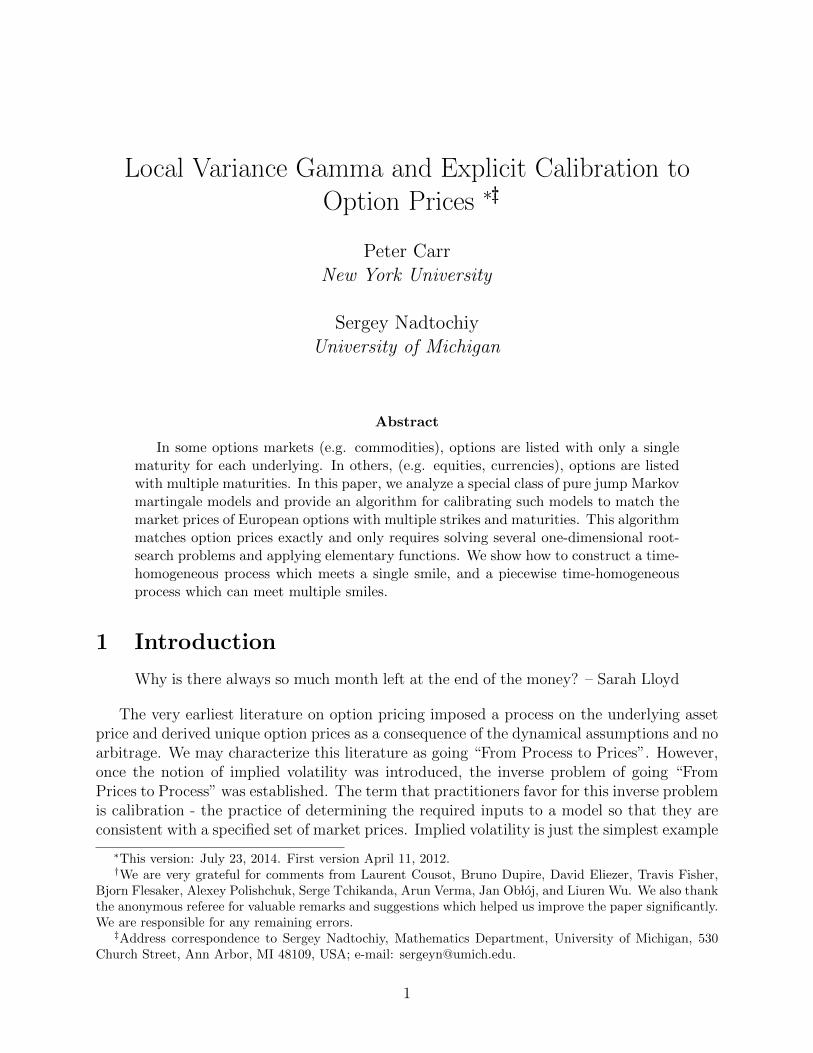
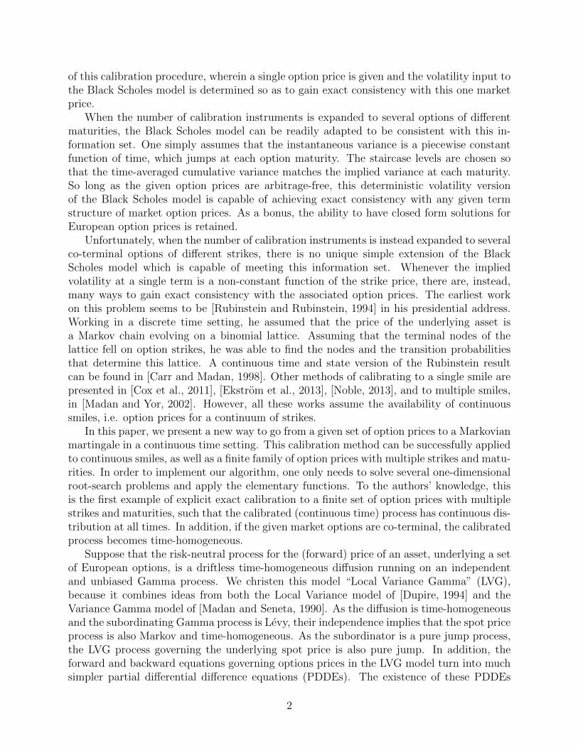
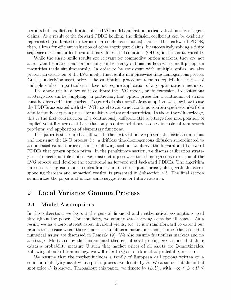
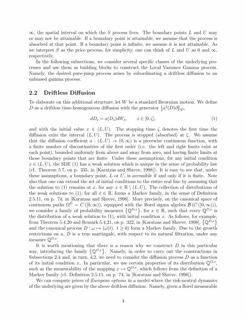
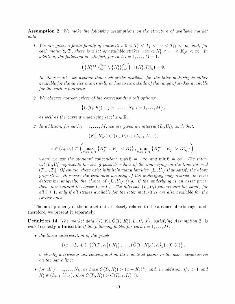
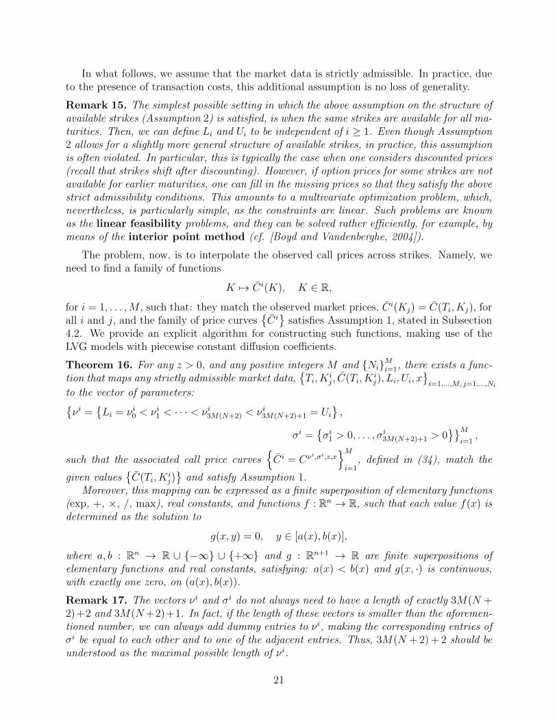
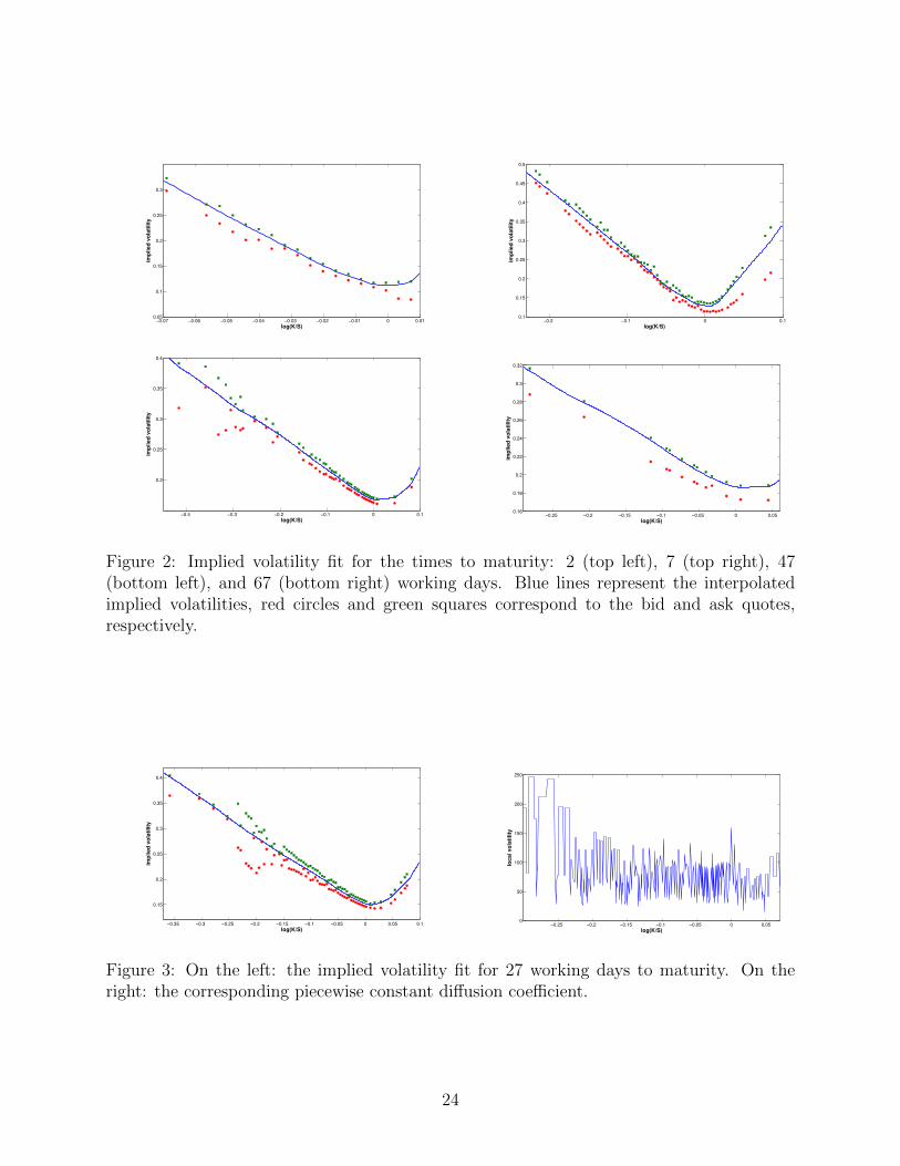
Figures 1–3 show the results of cross-maturity interpolation of the market prices of Eu-ropean options written on the S&P 500 index, on January 12, 20114. Figure 1 contains theresulting price curves of call options, as functions of strike. Each curve corresponds to adifferent maturity: 2, 7, 27, 47, and 67 working days, respectively. In particular, Figure 1demonstrates that the monotonicity of option prices across maturities is preserved by theinterpolation. The quality of the fit is shown on Figures 2–3, via the implied volatility curves.It is easy to see that the fit is perfect, in the sense that the implied volatility of interpolatedprices always falls within the implied volatilities of the bid and ask quotes.

It is worth mentioning that, in the given market data, the first part of Assumption 2is not satisfied. In particular, for longer maturities, the new strikes often appear betweenthe strikes that are available for shorter maturities. This occurs quite often, for example,because the option prices and strikes need to be adjusted for the non-zero dividend andinterest rates (cf. Remark 19). In addition, the market data contains bid and ask quotes, asopposed to exact prices. To resolve these issues, before initiating the calibration algorithm,we implement the method outlined in Remark 15. Namely, we solve a linear feasibilityproblem, to obtain a strictly admissible set of option prices, for the same strikes at everymaturity, such that the price of each option satisfies the given bid-ask constraints, if thisoption was traded in the market (i.e. the trading volume was positive) on that day.

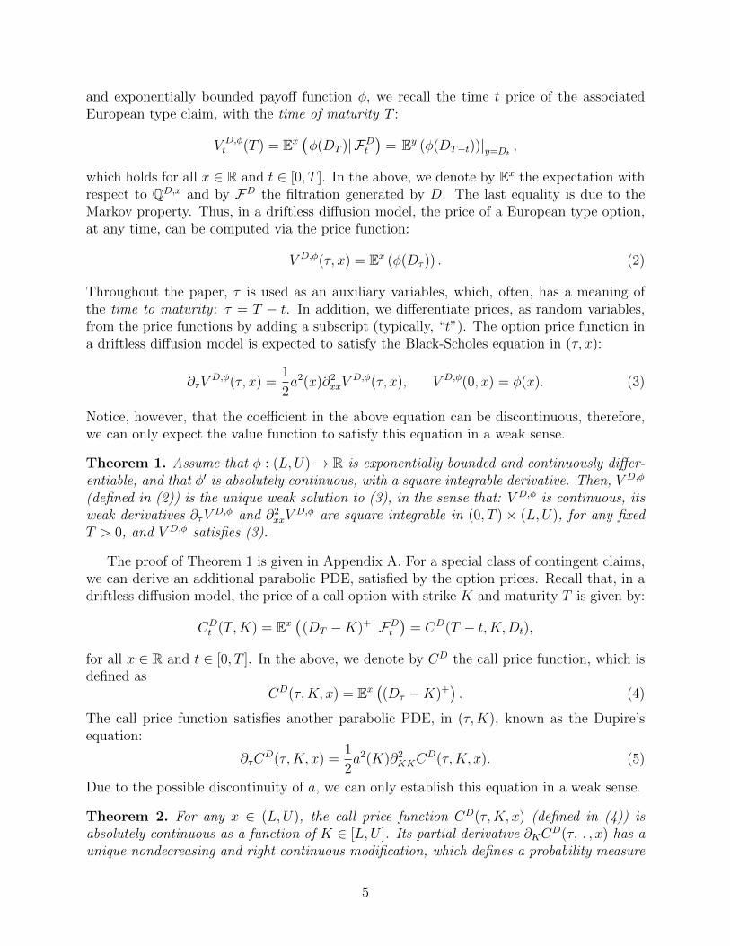
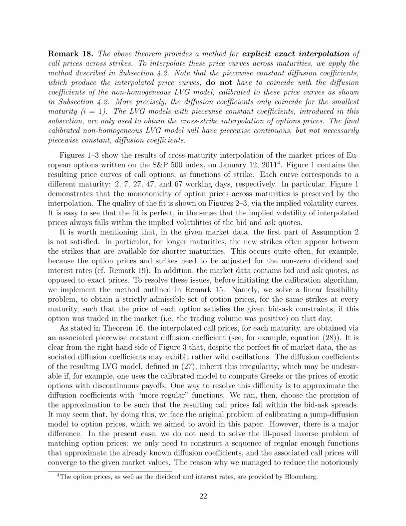
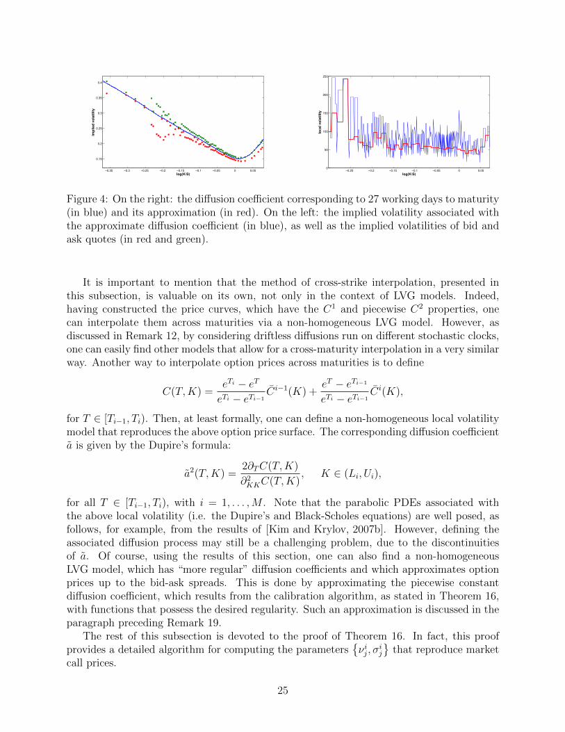
As stated in Theorem 16, the interpolated call prices, for each maturity, are obtained viaan associated piecewise constant diffusion coefficient (see, for example, equation (28)). It isclear from the right hand side of Figure 3 that, despite the perfect fit of market data, the as-sociated diffusion coefficients may exhibit rather wild oscillations. The diffusion coefficientsof the resulting LVG model, defined in (27), inherit this irregularity, which may be undesir-able if, for example, one uses the calibrated model to compute Greeks or the prices of exoticoptions with discontinuous payoffs. One way to resolve this difficulty is to approximate thediffusion coefficients with “more regular” functions. We can, then, choose the precision ofthe approximation to be such that the resulting call prices fall within the bid-ask spreads.It may seem that, by doing this, we face the original problem of calibrating a jump-diffusionmodel to option prices, which we aimed to avoid in this paper. However, there is a majordifference. In the present case, we do not need to solve the ill-posed inverse problem ofmatching option prices: we only need to construct a sequence of regular enough functionsthat approximate the already known diffusion coefficients, and the associated call prices willconverge to the given market values. The reason why we managed to reduce the notoriously

4The option prices, as well as the dividend and interest rates, are provided by Bloomberg.

22

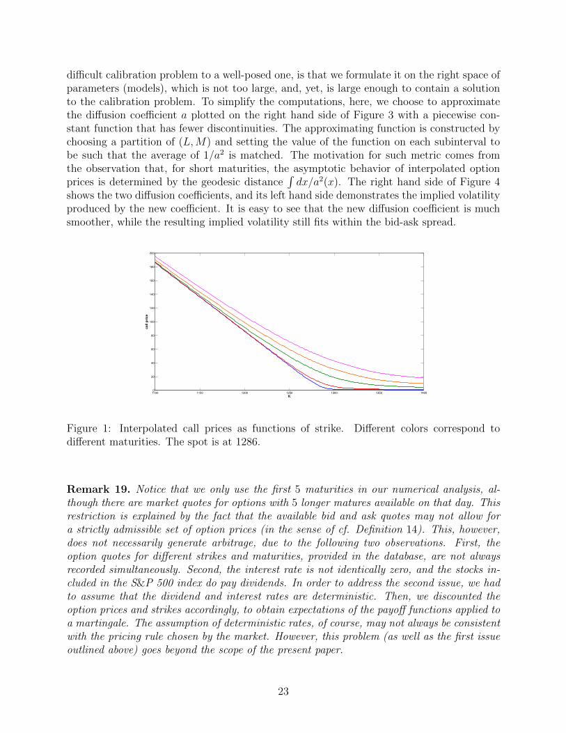
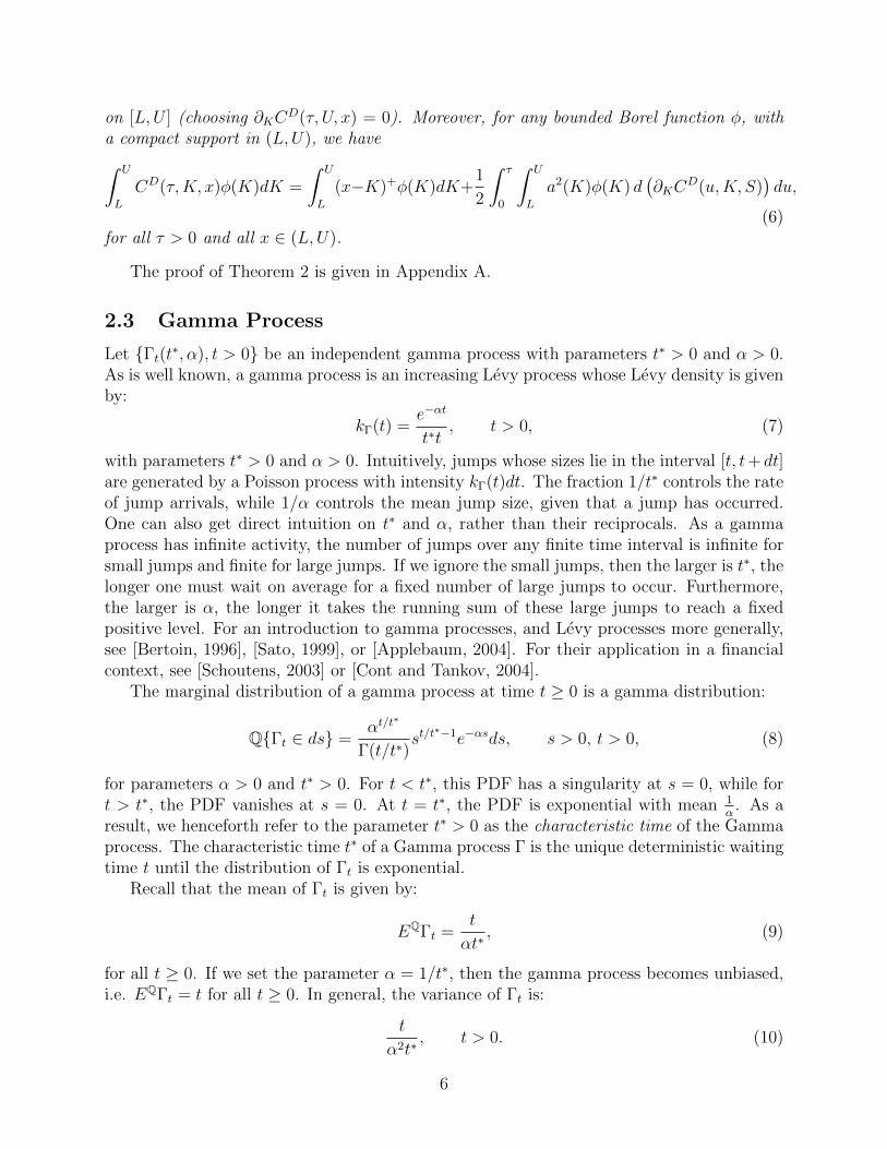
difficult calibration problem to a well-posed one, is that we formulate it on the right space ofparameters (models), which is not too large, and, yet, is large enough to contain a solutionto the calibration problem. To simplify the computations, here, we choose to approximatethe diffusion coefficient a plotted on the right hand side of Figure 3 with a piecewise con-stant function that has fewer discontinuities. The approximating function is constructed bychoosing a partition of (L,M) and setting the value of the function on each subinterval tobe such that the average of 1/a2 is matched. The motivation for such metric comes fromthe observation that, for short maturities, the asymptotic behavior of interpolated optionprices is determined by the geodesic distance

∫dx/a2(x). The right hand side of Figure 4

shows the two diffusion coefficients, and its left hand side demonstrates the implied volatilityproduced by the new coefficient. It is easy to see that the new diffusion coefficient is muchsmoother, while the resulting implied volatility still fits within the bid-ask spread.

1100 1150 1200 1250 1300 1350 14000

20

40

60

80

100

120

140

160

180

200

K

call p

rice

Figure 1: Interpolated call prices as functions of strike. Different colors correspond todifferent maturities. The spot is at 1286.

Remark 19. Notice that we only use the first 5 maturities in our numerical analysis, al-though there are market quotes for options with 5 longer matures available on that day. Thisrestriction is explained by the fact that the available bid and ask quotes may not allow fora strictly admissible set of option prices (in the sense of cf. Definition 14). This, however,does not necessarily generate arbitrage, due to the following two observations. First, theoption quotes for different strikes and maturities, provided in the database, are not alwaysrecorded simultaneously. Second, the interest rate is not identically zero, and the stocks in-cluded in the S&P 500 index do pay dividends. In order to address the second issue, we hadto assume that the dividend and interest rates are deterministic. Then, we discounted theoption prices and strikes accordingly, to obtain expectations of the payoff functions applied toa martingale. The assumption of deterministic rates, of course, may not always be consistentwith the pricing rule chosen by the market. However, this problem (as well as the first issueoutlined above) goes beyond the scope of the present paper.

23

−0.07 −0.06 −0.05 −0.04 −0.03 −0.02 −0.01 0 0.010.05

0.1

0.15

0.2

0.25

0.3

log(K/S)

imp

lied

vo

lati

lity

−0.2 −0.1 0 0.10.1

0.15

0.2

0.25

0.3

0.35

0.4

0.45

0.5

log(K/S)

imp

lied

vo

lati

lity

−0.4 −0.3 −0.2 −0.1 0 0.1

0.2

0.25

0.3

0.35

0.4

log(K/S)

imp

lied

vo

lati

lity

−0.25 −0.2 −0.15 −0.1 −0.05 0 0.050.16

0.18

0.2

0.22

0.24

0.26

0.28

0.3

0.32

log(K/S)

imp

lied

vo

lati

lity

Figure 2: Implied volatility fit for the times to maturity: 2 (top left), 7 (top right), 47(bottom left), and 67 (bottom right) working days. Blue lines represent the interpolatedimplied volatilities, red circles and green squares correspond to the bid and ask quotes,respectively.

−0.35 −0.3 −0.25 −0.2 −0.15 −0.1 −0.05 0 0.05 0.1

0.15

0.2

0.25

0.3

0.35

0.4

log(K/S)

imp

lied

vo

lati

lity

−0.25 −0.2 −0.15 −0.1 −0.05 0 0.050

50

100

150

200

250

log(K/S)

local vo

lati

lity

Figure 3: On the left: the implied volatility fit for 27 working days to maturity. On theright: the corresponding piecewise constant diffusion coefficient.

24

−0.35 −0.3 −0.25 −0.2 −0.15 −0.1 −0.05 0 0.05

0.15

0.2

0.25

0.3

0.35

0.4

log(K/S)

imp

lied

vo

lati

lity

−0.25 −0.2 −0.15 −0.1 −0.05 0 0.050

50

100

150

200

250

log(K/S)

local vo

lati

lity

Figure 4: On the right: the diffusion coefficient corresponding to 27 working days to maturity(in blue) and its approximation (in red). On the left: the implied volatility associated withthe approximate diffusion coefficient (in blue), as well as the implied volatilities of bid andask quotes (in red and green).

It is important to mention that the method of cross-strike interpolation, presented inthis subsection, is valuable on its own, not only in the context of LVG models. Indeed,having constructed the price curves, which have the C1 and piecewise C2 properties, onecan interpolate them across maturities via a non-homogeneous LVG model. However, asdiscussed in Remark 12, by considering driftless diffusions run on different stochastic clocks,one can easily find other models that allow for a cross-maturity interpolation in a very similarway. Another way to interpolate option prices across maturities is to define

C(T,K) =eTi − eT

eTi − eTi−1Ci−1(K) +

eT − eTi−1

eTi − eTi−1Ci(K),

for T ∈ [Ti−1, Ti). Then, at least formally, one can define a non-homogeneous local volatilitymodel that reproduces the above option price surface. The corresponding diffusion coefficienta is given by the Dupire’s formula:

a2(T,K) =2∂TC(T,K)

∂2KKC(T,K)

, K ∈ (Li, Ui),

for all T ∈ [Ti−1, Ti), with i = 1, . . . ,M . Note that the parabolic PDEs associated withthe above local volatility (i.e. the Dupire’s and Black-Scholes equations) are well posed, asfollows, for example, from the results of [Kim and Krylov, 2007b]. However, defining theassociated diffusion process may still be a challenging problem, due to the discontinuitiesof a. Of course, using the results of this section, one can also find a non-homogeneousLVG model, which has “more regular” diffusion coefficients and which approximates optionprices up to the bid-ask spreads. This is done by approximating the piecewise constantdiffusion coefficient, which results from the calibration algorithm, as stated in Theorem 16,with functions that possess the desired regularity. Such an approximation is discussed in theparagraph preceding Remark 19.

The rest of this subsection is devoted to the proof of Theorem 16. In fact, this proofprovides a detailed algorithm for computing the parameters

νij, σ

ij

that reproduce market

call prices.

25

Structure of the proof. The proof is presented in the form of an algorithm, which facil-itates the implementation. However, it is rather technical and uses a lot of new notation.Therefore, here, we outline the structure and the main ideas of the proof. It is easy to seethat any set of call price curves (as functions of strikes) produced by a family of homogeneousLVG models (different model for each curve), with piecewise constant diffusion coefficients,satisfies conditions 1 − 2 of Assumption 1. However, we still need to ensure that the LVGmodels are chosen so that the resulting price curves also satisfy part 3 of Assumption 1,which is a stronger version of the absence of calendar spread arbitrage. Thus, for each matu-rity Ti, we need to construct a piecewise constant diffusion coefficient ai and the associatedtime value function V i (which is uniquely defined by (29) and the subsequent paragraph),such that: each time value curve V i matches the time values observed in the market, andthe absence of calendar spread arbitrage is preserved (V i > V i−1, for all i). In order tomatch the observed market values, each V i is constructed recursively, passing from Kj toKj+1. This allows us to construct ai and V i locally, so that V i solves (29) on (Li, Kj+1),with ai in lieu of a. However, in order to obtain a bona fide time value function, we have toensure that V i satisfies the zero boundary conditions at Li and Ui, and has a jump of size−1 at x. These conditions force us to control the value of the left derivative of V i at eachstrike Kj, in addition to the value of V i(Kj) itself (which must coincide with the marketvalue). In order to satisfy the constraints on derivatives, along with the positivity of timevalue, we introduce two additional partition points between every Kj and Kj+1. The choiceof the additional partition points, as well as the proof that they are sufficient to fulfill theaforementioned conditions, takes most of the proof of Theorem 16 (Steps 1.1-1.3). The proof,itself, has an inductive nature: with the induction performed over maturities, and, for everyfixed maturity, over strikes. We show that the results of each iteration possess the necessaryproperties to serve as the initial condition for the next iteration.Step 0. Let us denote the market time values by V :

V (Ti, Kij) = C(Ti, K

ij)− (x−Ki

j)+,

for i = 1, . . . ,M , j = 1, . . . , Ni. It is clear that matching the market call prices is equivalentto matching their time values. To simplify the notation, we add the strikes Ki

0 = Li andKiNi+1 = Ui, for all i = 1, . . . ,M , to the set of available market strikes, with the corresponding

market time values being zero (since, in the calibrated model, the underlying cannot leavethe interval [Li, Ui] by the time Ti). We will construct the interpolated price curves thatmatch the original market prices, along with these additional ones.

Our construction will be recursive in i, starting from i = 1. Assume that we haveconstructed the interpolated time values for each maturity Tm,

V m(K) = V νm,σm,z,x(K), K ∈ R,

with m = 0, . . . , i− 1. For m = 0, we set V 0 ≡ 0. In addition to matching the market timevalues, we assume that these functions satisfy:

V m(K) > V m−1(K), K ∈ (Lm, Um),

for m = 1, . . . , i− 1, and V i−1 is strictly smaller than the market time values for maturitiesTi and larger. Our goal now is to construct V i = V νi,σi,z,x, such that the extended familyV mim=1 still satisfies the above monotonicity properties.

26

Without loss of generality, we can assume that the underlying level x coincides with oneof the strikes. If x is not among the available strikes, we can always add a new market callprice, for strike x and maturities T1, . . . , Ti, as follows: if x ∈ (Ki

j, Kij+1), then, we choose an

arbitrary δ1 ∈ (0, 1) and introduce the additional market time values

V (Tm, x) = V m(x), m = 1, . . . , i− 1,

V (Ti, x) = δ1

(C(Ti, K

ij

) Kij+1 − x

Kij+1 −Ki

j

+ C(Ti, K

ij+1

) x−Kij

Kij+1 −Ki

j

)+(1− δ1) max

(V i−1(x), C

(Ti, K

ij+1

)).

It is easy to see that the new family of market call prices, for m = i, . . . ,M , is strictlyadmissible, and the constructed time value functions, V 1, . . . , V i−1, satisfy the propertiesdiscussed in the previous paragraph, with respect to the new data.

The construction of V i(K) is done recursively in K, splitting the real line into severalsegments. We set V i(K) = 0, for all K ∈ (−∞, Li]. We, then, extend V i to each [Li, K

ij],

increasing j by one, as long as Kij+1 < x.

Step 1. Assume that Kij+1 < x and that, for all K ∈ [Li, K

ij], we have constructed the

time value function V i(K) in the form (30), with someLi = ν0 < · · · < νl(j) = Ki

j

and

σ1 > 0, . . . , σl(j) > 0

. In addition, we assume that V i(K) > V i−1(K), for all K ∈ [Li, Kij],

and the left derivative of V i(K) at K = Kij, denoted B, satisfies:

B <V (Ti, K

ij+1)− V (Ti, K

ij)

Kij+1 −Ki

j

. (35)

We need to extend V i to [Li, Kij+1] in such a way that: it remains in the form (30), on this

interval, it matches the market time value at Kij+1, and its left derivative at Ki

j+1 satisfiesthe above inequality.

Note that the case j = 0 is not included in the above discussion. In this case, the leftderivative of V i at Ki

0 = Li is zero. However, the derivative of V i does not have to becontinuous at this point, hence, we can change its value to a positive number. We choosethis number as follows: fix an arbitrary δ2 ∈ (0, 1) and define

B = δ2V (Ti, K

i1)

Ki1 − Li

+ (1− δ2)V i−1+ (Li) , (36)

where V i−1+ is the right derivative of V i−1. Due to the strict admissibility of market data, as

well as the convexity of V i−1(K) for K ∈ [Li, x], and the fact that V i−1(Ki1) < V (Ti, K

i1), we

easily deduce that B given by (36) satisfies (35), with j = 0, and, in addition, B > V i−1+ (Li).

Step 1.1. Choose an arbitrary δ3 ∈ (0, 1), and define

B1 = δ3

V (Ti, Kij+2)− V (Ti, K

ij+1)

Kij+2 −Ki

j+1

+ (1− δ3)V (Ti, K

ij+1)− V (Ti, K

ij)

Kij+1 −Ki

j

.

This will be the target derivative of extended time value function V i(K) at K = Kij+1. To

match this value, we need to introduce an additional jump point for the associated diffusioncoefficients.

27

0 0.1 0.2 0.3 0.4 0.5 0.6 0.7 0.8 0.9 10

0.1

0.2

0.3

0.4

0.5

0.6

0.7

0.8

0.9

1

strike

pri

ce

Ki

jA

1 + B

1(K−K

i

j+1)

w

Ki

j+1

A + B(K−Ki

j)

0 0.1 0.2 0.3 0.4 0.5 0.6 0.7 0.8 0.9 10

0.1

0.2

0.3

0.4

0.5

0.6

0.7

0.8

0.9

1

strike

pri

ce

Ki

jy

Ki

j+1

A + B(K−Ki

j)

Vi−1

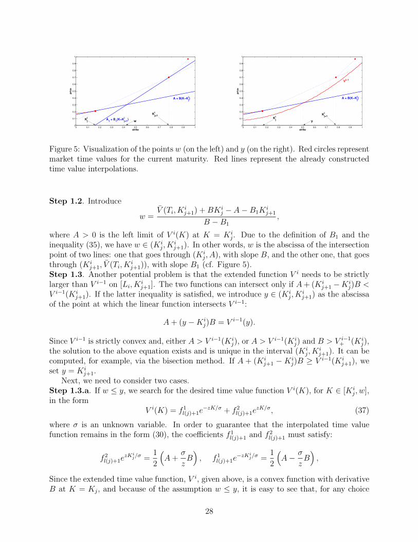
Figure 5: Visualization of the points w (on the left) and y (on the right). Red circles representmarket time values for the current maturity. Red lines represent the already constructedtime value interpolations.

Step 1.2. Introduce

w =V (Ti, K

ij+1) +BKi

j − A−B1Kij+1

B −B1

,

where A > 0 is the left limit of V i(K) at K = Kij. Due to the definition of B1 and the

inequality (35), we have w ∈ (Kij, K

ij+1). In other words, w is the abscissa of the intersection

point of two lines: one that goes through (Kij, A), with slope B, and the other one, that goes

through (Kij+1, V (Ti, K

ij+1)), with slope B1 (cf. Figure 5).

Step 1.3. Another potential problem is that the extended function V i needs to be strictlylarger than V i−1 on [Li, K

ij+1]. The two functions can intersect only if A+ (Ki

j+1 −Kij)B <

V i−1(Kij+1). If the latter inequality is satisfied, we introduce y ∈ (Ki

j, Kij+1) as the abscissa

of the point at which the linear function intersects V i−1:

A+ (y −Kij)B = V i−1(y).

Since V i−1 is strictly convex and, either A > V i−1(Kij), or A > V i−1(Ki

j) and B > V i−1+ (Ki

j),the solution to the above equation exists and is unique in the interval (Ki

j, Kij+1). It can be

computed, for example, via the bisection method. If A + (Kij+1 −Ki

j)B ≥ V i−1(Kij+1), we

set y = Kij+1.

Next, we need to consider two cases.Step 1.3.a. If w ≤ y, we search for the desired time value function V i(K), for K ∈ [Ki

j, w],in the form

V i(K) = f 1l(j)+1e

−zK/σ + f 2l(j)+1e

zK/σ, (37)

where σ is an unknown variable. In order to guarantee that the interpolated time valuefunction remains in the form (30), the coefficients f 1

l(j)+1 and f 2l(j)+1 must satisfy:

f 2l(j)+1e

zKij/σ =

1

2

(A+

σ

zB), f 1

l(j)+1e−zKi

j/σ =1

2

(A− σ

zB),

Since the extended time value function, V i, given above, is a convex function with derivativeB at K = Kj, and because of the assumption w ≤ y, it is easy to see that, for any choice

28

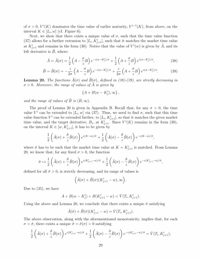
of σ > 0, V i(K) dominates the time value of earlier maturity, V i−1(K), from above, on theinterval K ∈ [Li, w] (cf. Figure 6).

Next, we show that there exists a unique value of σ, such that the time value function(37) allows for a further extension to [Li, K

ij+1], such that it matches the market time value

at Kij+1 and remains in the form (30). Notice that the value of V i(w) is given by A, and its

left derivative is B, where:

A = A(σ) =1

2

(A− σ

zB)e−z(w−K

ij)/σ +

1

2

(A+

σ

zB)ez(w−K

ij)/σ, (38)

B = B(σ) = − z

2σ

(A− σ

zB)e−z(w−K

ij)/σ +

z

2σ

(A+

σ

zB)ez(w−K

ij)/σ. (39)

Lemma 20. The functions A(σ) and B(σ), defined in (38)-(39), are strictly decreasing inσ > 0. Moreover, the range of values of A is given by(

A+B(w −Kij),∞

),

and the range of values of B is (B,∞).

The proof of Lemma 20 is given in Appendix B. Recall that, for any σ > 0, the timevalue V i can be extended to [Li, w] via (37). Thus, we need to find σ, such that this timevalue function V i can be extended further, to [Li, K

ij+1], so that it matches the given market

time value, and the target derivative, B1, at Kij+1. Since V i(K) remains in the form (30),

on the interval K ∈ [w,Kij+1], it has to be given by

1

2

(A(σ) +

σ

zB(σ)

)ez(K−w)/σ +

1

2

(A(σ)− σ

zB(σ)

)e−z(K−w)/σ,

where σ has to be such that the market time value at K = Kij+1 is matched. From Lemma

20, we know that, for any fixed σ > 0, the function

σ 7→ 1

2

(A(σ) +

σ

zB(σ)

)ez(K

ij+1−w)/σ +

1

2

(A(σ)− σ

zB(σ)

)e−z(K

ij+1−w)/σ,

defined for all σ > 0, is strictly decreasing, and its range of values is(A(σ) + B(σ)(Ki

j+1 − w),∞).

Due to (35), we have

A+B(w −Kij) +B(Ki

j+1 − w) < V (Ti, Kij+1).

Using the above and Lemma 20, we conclude that there exists a unique σ satisfying

A(σ) + B(σ)(Kij+1 − w) = V (Ti, K

ij+1).

The above observation, along with the aforementioned monotonicity, implies that, for eachσ > σ, there exists a unique σ = σ(σ) > 0 satisfying

1

2

(A(σ) +

σ

zB(σ)

)ez(K

ij+1−w)/σ +

1

2

(A(σ)− σ

zB(σ)

)e−z(K

ij+1−w)/σ = V (Ti, K

ij+1),

29

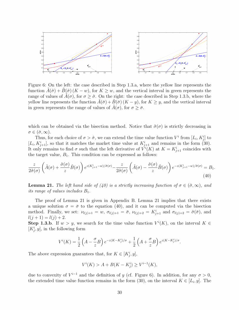
0 0.1 0.2 0.3 0.4 0.5 0.6 0.7 0.8 0.9 10

0.1

0.2

0.3

0.4

0.5

0.6

0.7

0.8

0.9

1

strike

pri

ce

w

Vi−1

Ki

j+1A

1 + B

1(K−K

i

j+1)

A + B(K−Ki

j)

Ki

j

0 0.1 0.2 0.3 0.4 0.5 0.6 0.7 0.8 0.9 10

0.1

0.2

0.3

0.4

0.5

0.6

0.7

0.8

0.9

1

strike

pri

ce

A + B(K−Ki

j)

yw

Ki

j+1Vi−1

A1 + B

1(K−K

i

j+1)

Ki

j

Figure 6: On the left: the case described in Step 1.3.a, where the yellow line represents thefunction A(σ) + B(σ) (K − w), for K ≥ w, and the vertical interval in green represents therange of values of A(σ), for σ ≥ σ. On the right: the case described in Step 1.3.b, where theyellow line represents the function A(σ) + B(σ) (K − y), for K ≥ y, and the vertical intervalin green represents the range of values of A(σ), for σ ≥ σ.

which can be obtained via the bisection method. Notice that σ(σ) is strictly decreasing inσ ∈ (σ,∞).

Thus, for each choice of σ > σ, we can extend the time value function V i from [Li, Kij] to

[Li, Kij+1], so that it matches the market time value at Ki

j+1 and remains in the form (30).It only remains to find σ such that the left derivative of V i(K) at K = Ki

j+1 coincides withthe target value, B1. This condition can be expressed as follows:

z

2σ(σ)

(A(σ) +

σ(σ)

zB(σ)

)ez(K

ij+1−w)/σ(σ)− z

2σ(σ)

(A(σ)− σ(σ)

zB(σ)

)e−z(K

ij+1−w)/σ(σ) = B1.

(40)

Lemma 21. The left hand side of (40) is a strictly increasing function of σ ∈ (σ,∞), andits range of values includes B1.

The proof of Lemma 21 is given in Appendix B. Lemma 21 implies that there existsa unique solution σ = σ to the equation (40), and it can be computed via the bisectionmethod. Finally, we set: νl(j)+1 = w, σl(j)+1 = σ, νl(j)+2 = Ki

j+1 and σl(j)+2 = σ(σ), andl(j + 1) = l(j) + 2.Step 1.3.b. If w > y, we search for the time value function V i(K), on the interval K ∈[Ki

j, y], in the following form

V i(K) =1

2

(A− σ

zB)e−z(K−K

ij)/σ +

1

2

(A+

σ

zB)ez(K−K

ij)/σ.

The above expression guarantees that, for K ∈ [Kij, y],

V i(K) > A+B(K −Kij) ≥ V i−1(K),

due to convexity of V i−1 and the definition of y (cf. Figure 6). In addition, for any σ > 0,the extended time value function remains in the form (30), on the interval K ∈ [Li, y]. The

30

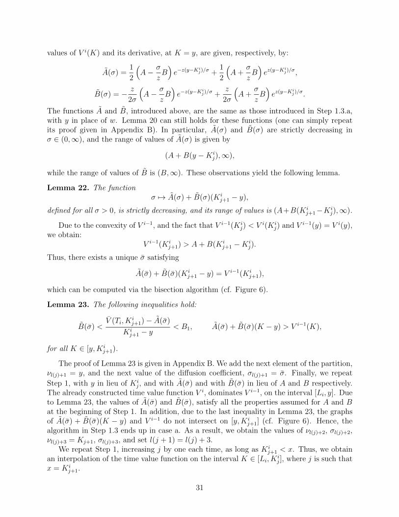
values of V i(K) and its derivative, at K = y, are given, respectively, by:

A(σ) =1

2

(A− σ

zB)e−z(y−K

ij)/σ +

1

2

(A+

σ

zB)ez(y−K

ij)/σ,

B(σ) = − z

2σ

(A− σ

zB)e−z(y−K

ij)/σ +

z

2σ

(A+

σ

zB)ez(y−K

ij)/σ.

The functions A and B, introduced above, are the same as those introduced in Step 1.3.a,with y in place of w. Lemma 20 can still holds for these functions (one can simply repeatits proof given in Appendix B). In particular, A(σ) and B(σ) are strictly decreasing inσ ∈ (0,∞), and the range of values of A(σ) is given by

(A+B(y −Kij),∞),

while the range of values of B is (B,∞). These observations yield the following lemma.

Lemma 22. The functionσ 7→ A(σ) + B(σ)(Ki

j+1 − y),

defined for all σ > 0, is strictly decreasing, and its range of values is (A+B(Kij+1−Ki

j),∞).

Due to the convexity of V i−1, and the fact that V i−1(Kij) < V i(Ki

j) and V i−1(y) = V i(y),we obtain:

V i−1(Kij+1) > A+B(Ki

j+1 −Kij).

Thus, there exists a unique σ satisfying

A(σ) + B(σ)(Kij+1 − y) = V i−1(Ki

j+1),

which can be computed via the bisection algorithm (cf. Figure 6).

Lemma 23. The following inequalities hold:

B(σ) <V (Ti, K

ij+1)− A(σ)

Kij+1 − y

< B1, A(σ) + B(σ)(K − y) > V i−1(K),

for all K ∈ [y,Kij+1).

The proof of Lemma 23 is given in Appendix B. We add the next element of the partition,νl(j)+1 = y, and the next value of the diffusion coefficient, σl(j)+1 = σ. Finally, we repeat

Step 1, with y in lieu of Kij, and with A(σ) and with B(σ) in lieu of A and B respectively.

The already constructed time value function V i, dominates V i−1, on the interval [Li, y]. Dueto Lemma 23, the values of A(σ) and B(σ), satisfy all the properties assumed for A and Bat the beginning of Step 1. In addition, due to the last inequality in Lemma 23, the graphsof A(σ) + B(σ)(K − y) and V i−1 do not intersect on [y,Ki

j+1] (cf. Figure 6). Hence, thealgorithm in Step 1.3 ends up in case a. As a result, we obtain the values of νl(j)+2, σl(j)+2,νl(j)+3 = Kj+1, σl(j)+3, and set l(j + 1) = l(j) + 3.

We repeat Step 1, increasing j by one each time, as long as Kij+1 < x. Thus, we obtain

an interpolation of the time value function on the interval K ∈ [Li, Kij], where j is such that

x = Kij+1.

31

Step 2. Perform Step 1, moving from K = Ui backwards. Namely, we consider the changeof variables: from K ∈ [Li, Ui] to K ′ = Li + Ui − K ∈ [Li, Ui]. We apply this change ofvariables to the market time values, as well as to the interpolated time value functions forearlier maturities. In particular, we obtain the new underlying level x′ = Li +Ui−x, as wellas the new market time values V (Ti, Li + Ui −K ′j), for all strikes K ′j = Li + Ui −Ki

Ni+1−j,with j = 0, . . . , Ni + 1. Then, we repeat Step 1, using this new, modified, data as an input.This gives us an interpolated time value function on the interval K ′ ∈ [Li, K

′j], where j is

such that x′ = K ′j+1. In the original variables, we obtain an interpolation of the time valuefunction on the interval K ∈ [Ki

Ni+1−j, Ui], where, in turn, x = KiNi−j. It is easy to see that

the interpolated time value, on the interval [KiNi+1−j, Ui], is in the form (32).

Step 3. Finally, we extend the interpolated time value function to the entire interval [Li, Ui].Recall that x coincides with one of the strikes, say Ki

j. In Steps 1 and 2, we constructedthe interpolated time value function for K ∈ [Li, K

ij−1] ∪ [Ki

j+1, Ui]. Notice that, repeatingthe algorithm outlined in Steps 1 and 2, we can extend V i to the entire interval [Li, Ui], sothat it matches all market time values, dominates V i−1 from above, and, in addition, it isin the form (30) on [Li, x], in the form (32) on [x, Ui], and it has the prescribed left andright derivatives at x, B1 and B2 respectively. In order for the interpolation function V i

to be a bona fide time value, it needs to have a jump of size −1 at x. In other words, weneed to choose B1 and B2 so that B1 − 1 = B2. The only constraints on the choices of B1

and B2 come from the market data and the previous constructed interpolation function onK ∈ [Li, K

ij−1] ∪ [Ki

j+1, Ui]. These constraints are given by:

B1 >V (Ti, K

ij)− V (Ti, K

ij−1)

Kij −Ki

j−1

, B2 <V (Ti, K

ij+1)− V (Ti, K

ij)

Kij+1 −Ki

j

=C(Ti, K

ij+1)− C(Ti, K

ij)

Kij+1 −Ki

j

.

(41)Thus, we choose an arbitrary δ4 ∈ (0, 1) and define

B1 = δ4 + δ4

V (Ti, Kij+1)− V (Ti, K

ij)

Kij+1 −Ki

j

+ (1− δ4)V (Ti, K

ij)− V (Ti, K

ij−1)

Kij −Ki

j−1

= δ4

C(Ti, Kij+1)− C(Ti, K

ij)

Kij+1 −Ki

j

− δ4

C(Ti, Kij)− C(Ti, K

ij−1)

Kij −Ki

j−1

+V (Ti, K

ij)− V (Ti, K

ij−1)

Kij −Ki

j−1

.

Similarly, we define

B2 = B1 − 1 = δ4 − 1 + δ4

V (Ti, Kij+1)− V (Ti, K

ij)

Kij+1 −Ki

j

+ (1− δ4)V (Ti, K

ij)− V (Ti, K

ij−1)

Kij −Ki

j−1

= δ4

C(Ti, Kij+1)− C(Ti, K

ij)

Kij+1 −Ki

j

+ (1− δ4)C(Ti, K

ij)− C(Ti, K

ij−1)

Kij −Ki

j−1

.

As the market call prices are strictly admissible (in particular, strictly convex across strikes),we conclude that B1 and B2 satisfy (41).

The following lemma, whose proof is given in Appendix B, completes the proof of thetheorem.

32

Lemma 24. For any z > 0 and any strictly admissible market data,Ti, K

ij, C(Ti, K

ij), Li, Ui, x

,

the vectors νi and σi, for i = 1, . . . ,M , produced by the above algorithm (Steps 0 − 3) are

such that the associated price curvesCi = Cνi,σi,z,x

Mi=1

satisfy Assumption 1.

Remark 25. Notice that the constants δi, for i = 1, 2, 3, 4, appearing in the proof, can bechosen arbitrarily (within the interval (0, 1)). The choice of the boundary points Li, Uiintroduces additional flexibility in the algorithm. It is worth mentioning that the proper-ties of interpolated implied volatilities and the associated diffusion coefficients may dependon the choices of these constants. Therefore, one may try to optimize over different valuesof δi and Li, Ui, for example, to improve the smoothness of resulting diffusion coeffi-cients. Continuing along these lines, one may also want to iterate over all possible choicesof arbitrage-free option prices, consistent with the market. Recall that the market data con-tains only bid and ask quotes, and we propose to choose the exact values of option prices bysolving a linear feasibility problem (cf. Remark 15). Optimizing over all possible choices ofoption prices, in theory, may improve the smoothness properties of the output. However, thiswould come at a very high computational cost, and would lead to a multivariate nonlinearoptimization problem, which we tried to avoid in the present paper.

5 Summary and Extensions

In this paper, we considered the risk-neutral process for the (forward) price of an asset,underlying a set of European options, in the form of a driftless time-homogeneous diffusionsubordinated to an unbiased gamma process. We named this model LVG and showed that ityields forward and backward PDDEs for option prices. These PDDEs can be used to speed upthe computations, but, more importantly, they allow for explicit exact calibration of a LVGmodel to European options prices. In particular, the diffusion coefficient of the underlyingcan be represented explicitly through a single (continuous) implied volatility smile. A mildextension of LVG allows for analogous calibration to multiple continuous smiles. Finally, weshowed how the aforementioned PDDEs can be used to construct continuously differentiable(with piecewise continuous second derivative) arbitrage-free implied volatility smiles from afinite set of option prices, with multiple strikes and maturities. The resulting calibrationalgorithm does not involve any multivariate optimization, and it only requires solutions toone-dimensional root-search problems and elementary functions. We illustrated the theorywith numerical results based on a real market data.

There are many possible avenues for future research. One of the potential criticisms ofthe proposed calibration method is the fact that the resulting diffusion coefficient has (afinite number of) discontinuities. This feature may create difficulties when computing thegreeks, or prices of path-dependent and American-style options in the calibrated model. Anidea on how to resolve this problem is outlined briefly in the few paragraphs preceding theproof of Theorem 16. However, a more detailed analysis would be very useful.

Another limitation of the results presented herein is that the risk-neutral price processof the underlying is assumed to be a martingale. Indeed, in many cases, the dividendand interest rates are not negligible. If they are assumed to be deterministic, then, thecalibration problem can be easily reduced to the driftless case by discounting. However, as

33

discussed in Remark 19, the assumption of deterministic rates may not be consistent withthe market. Therefore, an extension of the proposed model that allows for a non-zero driftof the underlying is very desirable. In particular, it seems possible to extend the resultsof this paper to a risk-neutral price process obtained as a time change of a diffusion withdrift. However, certain challenges may arise and they need to be addressed: in particular,the associated PDDEs may no longer have closed form solutions even if the diffusion anddrift coefficients are piecewise constant.

A more thorough numerical analysis, in particular, investigating the prices of exoticproducts produced by the calibrated models, is also very desirable. We did not conduct sucha study in the present paper, due to its already quite extensive length.

Finally, one can examine the problem of calibrating a LVG model to other financialinstruments, such as the barrier or American options.

Appendix A

Proof of Theorem 1. Theorems 2.2 and 2.7 in [Kim and Krylov, 2007b], as well as Theorem1.II in [Campanato, 1968] (a respective theorem is applicable depending on whether each ofthe boundary points is finite) provide existence and uniqueness results for a class of parabolicPDEs with initial and boundary conditions. This class includes the following equation:

∂τu(τ, x) =1

2a2(x)∂2

xu(τ, x) +1

2a2(x)φ′′(x), u(0, x) = u(τ, L+) = u(τ, U−) = 0,

implying that it has a unique weak solution. In addition u is absolutely bounded by a con-stant (which follows from the estimates in Theorems 2.2 and 2.7, in [Kim and Krylov, 2007b],and in Theorem 1.II, in [Campanato, 1968]), and it is vanishing at L and U . Then, v = u+φsolves (3) and satisfies v(0, x) = φ(x). In addition, it satisfies: v(τ, L+) = φ(L+) and/orv(τ, U−) = φ(U−), whenever L and/or U are finite. To show that this solution coincideswith V D,φ, we apply the generalized Ito’s formula (cf. Theorem 2.10.1 in [Krylov, 1980]), toobtain

Exv(T − ζr,R ∧ T,Dζr,R∧T ) = v(T, x),

where ζr,R is the first exit time of D from the interval (r, R), with arbitrary L < r < R < U .Notice that v(τ, x) is bounded by an exponential of x, uniformly over τ ∈ (0, T ). Thus, wecan apply the dominated convergence theorem, to conclude that, as r ↓ L and R ↑ U ,

v(T, x) = Exv(T − ζr,R ∧ T,Dζr,R∧T )→ Exv(T − ζ ∧ T,Dζ∧T )

= Exv(T − ζ,Dζ)1ζ≤T + Exφ(DT )1ζ>T,

where ζ is the time of the first exit of D from (L,U). Recall that the diffusion can only exitthe interval (L,U) through a finite boundary point. Thus,

v (T − ζ,Dζ) 1ζ≤T = v (T − ζ, L+) 1ζ≤T,Dζ=L+ + v (T − ζ, U−) 1ζ≤T,Dζ=U−

= φ(L+)1ζ≤T,Dζ=L+ + φ(U−)1ζ≤T,Dζ=U− = φ(Dζ)1ζ≤T.

34

As the diffusion is absorbed at the boundary points, we have:

v(T, x) = Ex(φ(DT )1ζ>T

)+ Ex

(φ(Dζ)1ζ≤T

)= Ex

(φ(DT )1ζ>T

)+ Ex

(φ(DT )1ζ≤T

)= Exφ(DT ),

which completes the proof of the theorem.Proof of Theorem 2. Let us apply the Ito-Tanaka rule (cf. Theorem 7.1, on page 218,

in [Karatzas and Shreve, 1998]) to the call payoff:

(Dt −K)+ = (D0 −K)+ +

∫ t

0

a(Ds)1Ds≥KdWs + Λt(K),

where Λ is the local time of D. Taking expectations, we obtain

CD(t,K, x) = Ex(Dt −K)+ = (x−K)+ + EΛt(K).

Multiplying by φ and integrating, we use the properties of local time (cf. Theorem 7.1, onpage 218, in [Karatzas and Shreve, 1998]), to obtain∫ U

L

CD(t,K, x)φ(K)dK =

∫ U

L

(x−K)+φ(K)dK +1

2

∫ t

0

Ex(a2(Du)φ(Du)

)du.

Using Fubini’s theorem, we obtain the following identity:

QD,x(Du ≤ K) = Ex1Du≤K = ∂KCD(u,K, x),

which holds for almost all K ∈ (L,U). Therefore, the measure generated by ∂KCD(u, ·, x)

is the distribution of Du under measure QD,x. Thus, we conclude:∫ U

L

CD(t,K, x)φ(K)dK =

∫ U

L

(x−K)+φ(K)dK+1

2

∫ t

0

∫ U

L

a2(K)φ(K)d(∂KC

D(u,K, x))du.

Proof of Theorem 6. Let us multiply the left hand side of equation (3) by the densityof Γt and an arbitrary test function ϕ ∈ C∞0 ((L,U)), then, divide it by a2/2 and integratewith respect to τ and x:∫ U

L

∫ T

0

τ t/t∗−1e−τ/t

∗

(t∗)t/t∗Γ(t/t∗)∂τV

D,φ(τ, x)2ϕ(x)

a2(x)dτdx

=

∫ U

L

∫ T

0

τ t/t∗−1e−τ/t

∗

(t∗)t/t∗Γ(t/t∗)∂τ(V D,φ(τ, x)− φ(x)

)dτ

2ϕ(x)

a2(x)dx

=T t/t

∗−1e−T/t∗

(t∗)t/t∗Γ(t/t∗)

∫ U

L

(V D,φ(T, x)− φ(x)

) 2ϕ(x)

a2(x)dx (42)

−∫ T

0

((t/t∗ − 1)τ t/t

∗−2 − τ t/t∗−1/t∗)e−τ/t

∗

(t∗)t/t∗Γ(t/t∗)

∫ U

L

(V D,φ(τ, x)− φ(x)

) 2ϕ(x)

a2(x)dxdτ

→∫ U

L

∫ ∞0

(τ t/t

∗−1/t∗ − (t/t∗ − 1)τ t/t∗−2)e−τ/t

∗

(t∗)t/t∗Γ(t/t∗)

(V D,φ(τ, x)− φ(x)

)dτ

2ϕ(x)

a2(x)dx,

35

as T →∞. In the above, we applied Fubini’s theorem and used the fact that φ is absolutelybounded and, hence, so is V D,φ. Recall also that τ ≥ t∗. Applying Fubini’s theorem oncemore, we interchange the order of integration in the left hand side of (42), and, using equation(3), integrate by parts with respect to x. This, together with the convergence in (42), implies:∫ ∞

0

τ t/t∗−1e−τ/t

∗

(t∗)t/t∗Γ(t/t∗)

∫ U

L

V D,φ(τ, x)ϕ′′(x)dxdτ (43)

=

∫ U

L

∫ ∞0

(τ t/t

∗−1/t∗ − (t/t∗ − 1)τ t/t∗−2)e−τ/t

∗

(t∗)t/t∗Γ(t/t∗)

(V D,φ(τ, x)− φ(x)

)dτ

2

a2(x)ϕ(x)dx,

where both integrals are absolutely convergent. Using Fubini’s theorem and the definitionof V φ, we conclude that∫ ∞

0

τ t/t∗−1e−τ/t

∗

(t∗)t/t∗Γ(t/t∗)

∫ U

L

V D,φ(τ, x)ϕ′′(x)dxdτ =

∫ U

L

V φ(t, x)ϕ′′(x)dx. (44)

Next, we notice that, since t ≥ t∗, the expression inside the outer integral in the right handside of (43) is a locally integrable function of x ∈ (L,U). Then, the fact that equations (42)and (43) hold for all test functions ϕ yields:

∂2xxV

φ(t, x) =2

a2(x)

∫ ∞0

(τ t/t

∗−1/t∗ − (t/t∗ − 1)τ t/t∗−2)e−τ/t

∗

(t∗)t/t∗Γ(t/t∗)

(V D,φ(τ, x)− φ(x)

)dτ, (45)

which holds for every t ≥ t∗ and almost all x ∈ (L,U). Since the second derivative ofV φ(τ, ·) is locally integrable, its first derivative is absolutely continuous. To show thatV φ(τ, L+) = V φ(τ, U−) = 0, we recall the definition of V φ as an expectation and apply thedominated convergence theorem. When t = t∗, equation (45) becomes

∂2xxV

φ(t∗, x) =2

a2(x)t∗

∫ ∞0

e−τ/t∗

t∗(V D,φ(τ, x)− φ(x)

)dτ =

2

a2(x)t∗(V φ(t, x)− φ(x)

),

which holds for almost all x ∈ (L,U). Since V φ(τ, ·) and φ are continuous, the aboveequation holds for all points x at which a is continuous. Therefore, V φ(t∗, ·) possesses all theproperties stated in the theorem.

Next, we show uniqueness. Consider any function u ∈ C1(L,U), which has an absolutelycontinuous derivative and satisfies (20), along with zero boundary conditions. Applying thegeneralized Ito’s formula (cf. Theorem 2.10.1 in [Krylov, 1980]), we obtain:

u(Dt∧ζr,R)− u(D0) =

∫ t∧ζr,R

0

1

2a2(Ds)u

′′(Ds)ds+

∫ t∧ζr,R

0

u′(Ds)dDs,

where, as before, ζr,R is the first exit time of D from the interval (r, R), with arbitraryL < r < R < U . Notice that, since u is continuous and satisfies zero boundary conditions,it is absolutely bounded. Due to equation (20), u′′ is absolutely bounded as well. Thus,taking expectations and applying the dominated convergence theorem, as r ↓ L and R ↑ U ,we obtain

Exu(Dt)− u(x) = E∫ t

0

1

2a2(Ds)u

′′(Ds)1s≤ζds.

36

Since Γ is independent of D, we can plug Γt∗ , in place of t, into the above expression, toobtain:

Exu (DΓt∗ )− u(x) = Ex∫ Γt∗

0

1

2a2(Ds)u

′′(Ds)1s≤ζds,∫ ∞0

e−t/t∗

t∗Exu(Dt)dt− u(x) =

∫ ∞0

e−t/t∗

t∗Ex∫ t

0

1

2a2(Ds)u

′′(Ds)1s≤ζdsdt,∫ ∞0

e−t/t∗

t∗Exu(Dt)dt− u(x) =

∫ ∞0

e−t/t∗

t∗Ex∫ t

0

1

t∗(u(Ds)− φ(Ds)) 1s≤ζdsdt,∫ ∞

0

e−t/t∗

t∗Exu(Dt)dt− u(x) =

1

t∗

∫ ∞0

e−t/t∗

t∗

∫ t

0

Ex (u(Ds)− φ(Ds)) dsdt, (46)

where we made use of the fact that u(L+) = u(U−) = φ(L+) = φ(U−) = 0, to obtain (46).Thus, we continue:∫ ∞

0

e−t/t∗

t∗Exu(Dt)dt− u(x) =

1

t∗

∫ ∞0

e−t/t∗Ex (u(Dt)− φ(Dt)) dt, (47)

where we integrated by parts in the right hand side of (46), to obtain (47). This yields:

u(x) =1

t∗

∫ ∞0

e−t/t∗Exφ(Dt)dt = V φ(t∗, x).

Proof of Lemma 7. Let us show that St∗ has a density in (L,U) under any Qx.Consider arbitrary K ∈ (L,U) and ε ∈ (0, 1), s.t. [K − ε,K + 2ε] ⊂ (L,U). Choose asmooth function ρε, which dominates the indicator function of [K,K+ ε] from above, whosesupport is contained in [K − ε,K + 2ε], and which satisfies∫ U

L

ρ2ε(x)dx ≤ 2ε.

Introduceu(x) = Ex (ρε(St∗)) ,

for all x ∈ (L,U). Theorem 6 implies that u ∈ C1(L,U), u(L+) = u(U−) = 0, u′′ ∈ L2(L,U),and it satisfies:

1

2a2(x)u′′(x)− 1

t∗(u(x)− ρε(x)) = 0, (48)

for all x ∈ (L,U), except the points of discontinuity of a. Next, we need to recall the standardestimates for the weak solutions of elliptic PDEs via the norm of the right hand side (see,for example, [Kim and Krylov, 2007a] and references therein). The only issue that needs tobe resolved, before we can apply the standard results, is that, although u belongs to theSobolev space W 2

2 ((L,U)), it may not belong to W 22 (R). This is due to the fact that u′ may

have a discontinuity at L or U , if the boundary point is attainable. To resolve this problem,we consider a sequence of functions un ∈ C∞0 (R) ⊂ W 2

2 (R) which approximates u in the

37

sense of the Sobolev norm ‖ · ‖W 22 (L,U). Applying Remark 3.3, in [Kim and Krylov, 2007a],

to un and passing to the limit, as n→∞, we estimate the Sobolev norm of u:∫ U

L

u2(x) + (u′(x))2 + (u′′(x))2dx ≤ c1

∫ U

L

ρ2ε(x)dx, (49)

where the constant c1 is independent of ε. Next, the Morrey’s inequality yields

supx∈(L,U)

|u(x)| ≤ c2

(∫ U

L

u2(x) + (u′(x))2dx

)1/2

≤ c3

(∫ U

L

ρ2ε(x)dx

)1/2

≤ c3

√2ε.

Finally, we obtainQx(St∗ ∈ [K,K + ε]) ≤ u(x) ≤ c3

√2ε,

Therefore, the distribution of St∗ is absolutely continuous with respect to the Lebesguemeasure on (L,U) and, in particular, it has a density. It was shown in the proof of Theorem2 that

Qx(St∗ ≤ K) = ∂KC(t∗, K, x).

Therefore, ∂KC(t∗, K, x) is absolutely continuous inK ∈ (L,U), and its derivative, ∂2KKC(t∗, ·, x),

is the density of St∗ under Qx.Proof of Theorem 8. Differentiating both sides of (6) with respect to τ , then, multi-

plying them by an exponential and a test function ϕ ∈ C∞0 ((L,U)), we integrate, to obtain∫ T

0

e−τ/t∗

t∗d

dτ

∫ U

L

CD(τ,K, x)2

a2(K)ϕ(K)dKdτ =

∫ T

0

e−τ/t∗

t∗

∫ U

L

ϕ(K)d(∂KC

D(τ,K, x))dτ.

(50)Let us perform integration by parts in the left hand side of (50):∫ T

0

e−τ/t∗

t∗d

dτ

∫ U

L

CD(τ,K, x)2

a2(K)ϕ(K)dKdτ =

e−T/t∗

t∗

∫ U

L

CD(T,K, x)2

a2(K)ϕ(K)dK

− 1

t∗

∫ U

L

(x−K)+ 2

a2(K)ϕ(K)dK +

1

t∗

∫ T

0

e−τ/t∗

t∗

∫ U

L

CD(τ,K, x)2

a2(K)ϕ(K)dKdτ, (51)

where we made use of the fact that

limτ↓0

CD(τ,K, x) = (x−K)+,

which, in turn, follows from square integrability of the martingale D and the dominated con-vergence theorem. Using (51), as well as the dominated convergence and Fubini’s theorems,we obtain:

limT→∞

∫ T

0

e−τ/t∗

t∗d

dτ

∫ U

L

CD(τ,K, x)2

a2(K)ϕ(K)dKdτ

=

∫ U

L

2

a2(K)t∗(C(t∗, K, x)− (x−K)+

)ϕ(K)dK.

38

On the other hand, integrating by parts and applying the Fubini and dominated convergencetheorems once more, we derive:

limT→∞

∫ T

0

e−τ/t∗

t∗

∫ U

L

ϕ(K)d(∂KC

D(τ,K, x))dτ = lim

T→∞

∫ U

L

ϕ′′(K)

∫ T

0

e−τ/t∗

t∗CD(τ,K, x)dτdK

=

∫ U

L

C(t∗, K, x)ϕ′′(K)dK =

∫ U

L

∂2KKC(t∗, K, x)ϕ(K)dK.

Collecting the above, we rewrite equation (50) as∫ U

L

(1

t∗(C(t∗, K, x)− (x−K)+

)− 1

2a2(K)∂2

KKC(t∗, K, x)

)ϕ(K)dK = 0,

which holds for any ϕ ∈ C∞0 ((L,U)). This implies that equation (22) holds for almost everyK ∈ (L,U). Since C(t∗, ·, x) and (x − ·)+ are continuous functions, we conclude that (22)holds everywhere except the points of discontinuity of a.

The boundary conditions for call price function follow from the dominated convergencetheorem. The square integrability of ∂2

KKC(t∗, ·, x) follows from the fact that it is absolutelyintegrable and vanishes at the boundary (the latter, in turn, follows from the boundaryconditions and equation (22)). To show uniqueness, we assume that there exists anotherfunction, with the same properties, and denote the difference between the two by u. Functionu is a weak solution of the homogeneous version of (22):

1

2a2(x)u′′(x)− 1

t∗u(x) = 0,

vanishing at the boundary. Finally, as in the proof of Lemma 7, we apply Remark 3.3 in[Kim and Krylov, 2007a] to obtain an estimate for the Sobolev norm of u, analogous to (49),with zero in lieu of ρε. This implies that u ≡ 0.

Proof of Theorem 9. Notice that, for a fixed K ∈ (L,U), the function C(t∗, K, . ) ismeasurable. This follows from the measurability of CD(T,K, . ), which, in turn, follows fromthe measurability of the mapping x 7→ QD,x, as a property of Markov family. At any pointK ∈ (L,U) that does not coincide with a discontinuity point of a, the call price function istwice continuously differentiable in K, and, hence, its second derivative, ∂2

KKC(t∗, K, x), isalso measurable as a function of x. Thus, we can use (22) to obtain

1

t∗(ExC(t∗, K, Sτ )− Ex(Sτ −K)+

)=a2(K)

2Ex(∂2KKC(t∗, K, Sτ )

), (52)

which holds for all τ ≥ 0 and all K ∈ (L,U) except the points of discontinuity of a. Since∂2KKC(t∗, ·, Sτ ) is nonnegative and integrates to one, the application of Fubini’s theorem

yieldsEx(∂2KKC(t∗, K, Sτ )

)= ∂2

KKExC(t∗, K, Sτ ) = ∂2KKC(τ + t∗, K, x), (53)

where the derivatives in the right hand side are understood in a weak sense, and we usedProposition 5 to obtain the last equality. Due to (52), ∂2

KKC(τ + t∗, ·, x) is, in fact, locallyintegrable on (L,U), and equation (24) holds for almost every K ∈ (L,U). Using the

39

monotone convergence theorem, it is easy to show that C(τ, ·, x) is continuous, for anyτ ≥ 0, and, hence, (24) holds everywhere except the points of discontinuity of a. Theboundary conditions follow from the dominated convergence theorem. In addition, (53) andan application of Fubini’s theorem imply that ∂2

KKC(τ + t∗, ·, x) is absolutely integrable on(L,U). This, along with the boundary conditions and equation (24), imply that ∂2

KKC(τ +t∗, ·, x) is square integrable. To show uniqueness, we apply the same argument as at the endof the proof of Theorem 8.

Appendix B

Proof of Lemma 20. Notice that, for all y > 0, we have:((1 + y)e−2y + y − 1

)′= 1− e−2y(1 + 2y) > 0,

which follows from the inequality e2y > 1 + 2y. Since (1 + 0)e−2·0 + 0− 1 = 0, we obtain

(1 + y)e−2y + y − 1 > 0, y > 0.

Therefore, for any positive A and B,

A′(σ) =1

2

((A− σ

zB) z(w −Ki

j)

σ2− B

z

)e−z(w−K

ij)/σ

−1

2

((A+

σ

zB) z(w −Ki

j)

σ2− B

z

)ez(w−K

ij)/σ

=1

2

(Az(w −Ki

j)

σ2− B

z

(z(w −Ki

j)

σ+ 1

))e−z(w−K

ij)/σ

−1

2

(Az(w −Ki

j)

σ2+B

z

(z(w −Ki

j)

σ− 1

))ez(w−K

ij)/σ

=1

2Az(w −Ki

j)

σ2

(e−z(w−K

ij)/σ − ez(w−Ki

j)/σ)

−1

2

B

zez(w−K

ij)/σ

((z(w −Ki

j)

σ+ 1

)e−2z(w−Ki

j)/σ +

(z(w −Ki

j)

σ− 1

))≤ 0.

Similarly, we have:

B′(σ) = −1

2

(( zσA−B

) z(w −Kij)

σ2− z

σ2A

)e−z(w−K

ij)/σ

+1

2

(−( zσA+B

) z(w −Kij)

σ2− z

σ2A

)ez(w−K

ij)/σ

= − z

2σ2

(z(w −Ki

j)

σA−B(w −Ki

j)− A)e−z(w−K

ij)/σ

40

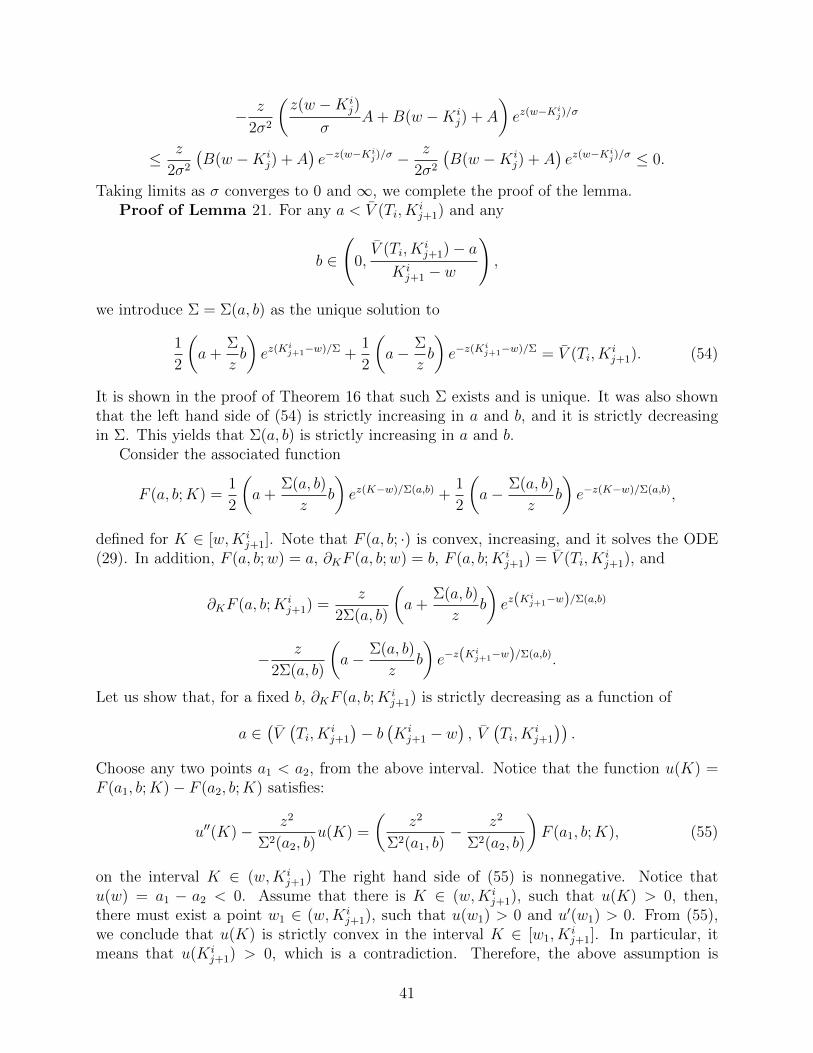
− z

2σ2

(z(w −Ki

j)

σA+B(w −Ki

j) + A

)ez(w−K

ij)/σ

≤ z

2σ2

(B(w −Ki

j) + A)e−z(w−K

ij)/σ − z

2σ2

(B(w −Ki

j) + A)ez(w−K

ij)/σ ≤ 0.

Taking limits as σ converges to 0 and ∞, we complete the proof of the lemma.Proof of Lemma 21. For any a < V (Ti, K

ij+1) and any

b ∈

(0,V (Ti, K

ij+1)− a

Kij+1 − w

),

we introduce Σ = Σ(a, b) as the unique solution to

1

2

(a+

Σ

zb

)ez(K

ij+1−w)/Σ +

1

2

(a− Σ

zb

)e−z(K

ij+1−w)/Σ = V (Ti, K

ij+1). (54)

It is shown in the proof of Theorem 16 that such Σ exists and is unique. It was also shownthat the left hand side of (54) is strictly increasing in a and b, and it is strictly decreasingin Σ. This yields that Σ(a, b) is strictly increasing in a and b.

Consider the associated function

F (a, b;K) =1

2

(a+

Σ(a, b)

zb

)ez(K−w)/Σ(a,b) +

1

2

(a− Σ(a, b)

zb

)e−z(K−w)/Σ(a,b),

defined for K ∈ [w,Kij+1]. Note that F (a, b; ·) is convex, increasing, and it solves the ODE

(29). In addition, F (a, b;w) = a, ∂KF (a, b;w) = b, F (a, b;Kij+1) = V (Ti, K

ij+1), and

∂KF (a, b;Kij+1) =

z

2Σ(a, b)

(a+

Σ(a, b)

zb

)ez(K

ij+1−w)/Σ(a,b)

− z

2Σ(a, b)

(a− Σ(a, b)

zb

)e−z(K

ij+1−w)/Σ(a,b).

Let us show that, for a fixed b, ∂KF (a, b;Kij+1) is strictly decreasing as a function of

a ∈(V(Ti, K

ij+1

)− b(Kij+1 − w

), V(Ti, K

ij+1

)).

Choose any two points a1 < a2, from the above interval. Notice that the function u(K) =F (a1, b;K)− F (a2, b;K) satisfies:

u′′(K)− z2

Σ2(a2, b)u(K) =

(z2

Σ2(a1, b)− z2

Σ2(a2, b)

)F (a1, b;K), (55)

on the interval K ∈ (w,Kij+1) The right hand side of (55) is nonnegative. Notice that

u(w) = a1 − a2 < 0. Assume that there is K ∈ (w,Kij+1), such that u(K) > 0, then,

there must exist a point w1 ∈ (w,Kij+1), such that u(w1) > 0 and u′(w1) > 0. From (55),

we conclude that u(K) is strictly convex in the interval K ∈ [w1, Kij+1]. In particular, it

means that u(Kij+1) > 0, which is a contradiction. Therefore, the above assumption is

41

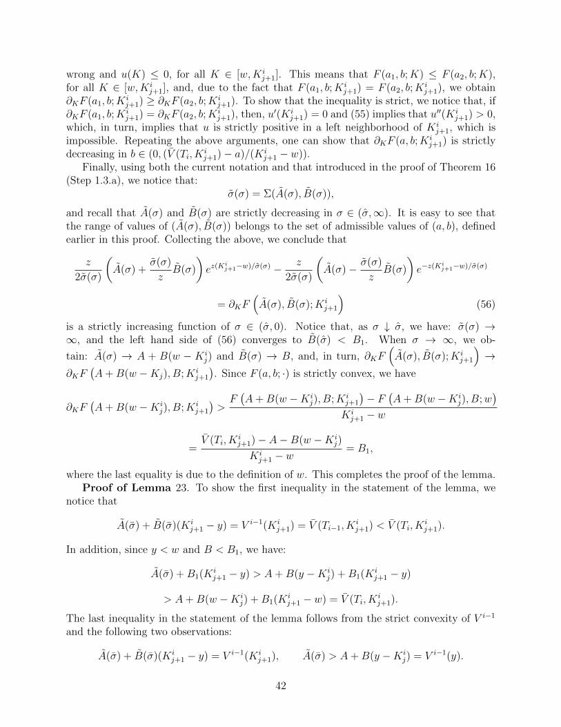
wrong and u(K) ≤ 0, for all K ∈ [w,Kij+1]. This means that F (a1, b;K) ≤ F (a2, b;K),

for all K ∈ [w,Kij+1], and, due to the fact that F (a1, b;K

ij+1) = F (a2, b;K

ij+1), we obtain

∂KF (a1, b;Kij+1) ≥ ∂KF (a2, b;K

ij+1). To show that the inequality is strict, we notice that, if

∂KF (a1, b;Kij+1) = ∂KF (a2, b;K

ij+1), then, u′(Ki

j+1) = 0 and (55) implies that u′′(Kij+1) > 0,

which, in turn, implies that u is strictly positive in a left neighborhood of Kij+1, which is

impossible. Repeating the above arguments, one can show that ∂KF (a, b;Kij+1) is strictly

decreasing in b ∈ (0, (V (Ti, Kij+1)− a)/(Ki

j+1 − w)).Finally, using both the current notation and that introduced in the proof of Theorem 16

(Step 1.3.a), we notice that:σ(σ) = Σ(A(σ), B(σ)),

and recall that A(σ) and B(σ) are strictly decreasing in σ ∈ (σ,∞). It is easy to see thatthe range of values of (A(σ), B(σ)) belongs to the set of admissible values of (a, b), definedearlier in this proof. Collecting the above, we conclude that

z

2σ(σ)

(A(σ) +

σ(σ)

zB(σ)

)ez(K

ij+1−w)/σ(σ) − z

2σ(σ)

(A(σ)− σ(σ)

zB(σ)

)e−z(K

ij+1−w)/σ(σ)

= ∂KF(A(σ), B(σ);Ki

j+1

)(56)

is a strictly increasing function of σ ∈ (σ, 0). Notice that, as σ ↓ σ, we have: σ(σ) →∞, and the left hand side of (56) converges to B(σ) < B1. When σ → ∞, we ob-

tain: A(σ) → A + B(w − Kij) and B(σ) → B, and, in turn, ∂KF

(A(σ), B(σ);Ki

j+1

)→

∂KF(A+B(w −Kj), B;Ki

j+1

). Since F (a, b; ·) is strictly convex, we have

∂KF(A+B(w −Ki

j), B;Kij+1

)>F(A+B(w −Ki

j), B;Kij+1

)− F

(A+B(w −Ki

j), B;w)

Kij+1 − w

=V (Ti, K

ij+1)− A−B(w −Ki

j)

Kij+1 − w

= B1,

where the last equality is due to the definition of w. This completes the proof of the lemma.Proof of Lemma 23. To show the first inequality in the statement of the lemma, we

notice that

A(σ) + B(σ)(Kij+1 − y) = V i−1(Ki

j+1) = V (Ti−1, Kij+1) < V (Ti, K

ij+1).

In addition, since y < w and B < B1, we have:

A(σ) +B1(Kij+1 − y) > A+B(y −Ki

j) +B1(Kij+1 − y)

> A+B(w −Kij) +B1(Ki

j+1 − w) = V (Ti, Kij+1).

The last inequality in the statement of the lemma follows from the strict convexity of V i−1

and the following two observations:

A(σ) + B(σ)(Kij+1 − y) = V i−1(Ki

j+1), A(σ) > A+B(y −Kij) = V i−1(y).

42

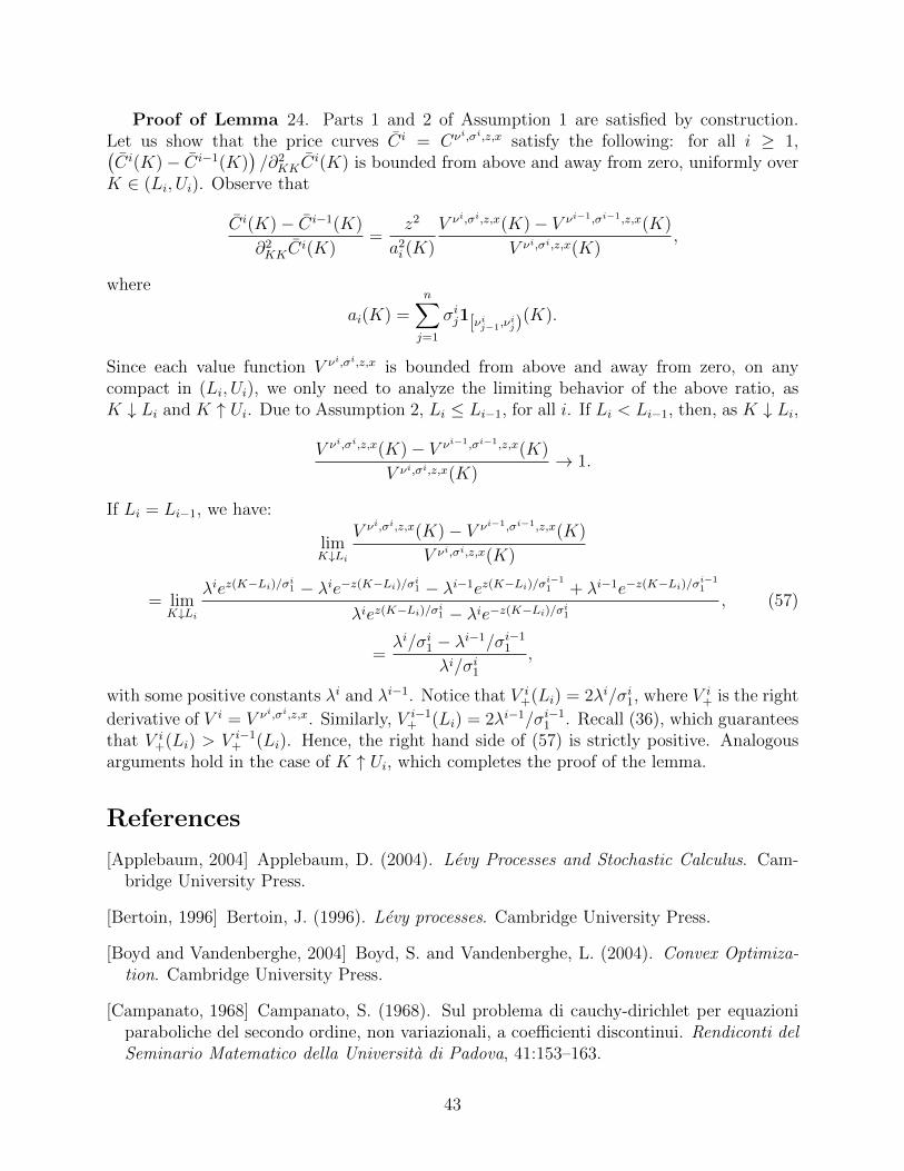
Proof of Lemma 24. Parts 1 and 2 of Assumption 1 are satisfied by construction.Let us show that the price curves Ci = Cνi,σi,z,x satisfy the following: for all i ≥ 1,(Ci(K)− Ci−1(K)

)/∂2

KKCi(K) is bounded from above and away from zero, uniformly over

K ∈ (Li, Ui). Observe that

Ci(K)− Ci−1(K)

∂2KKC

i(K)=

z2

a2i (K)

V νi,σi,z,x(K)− V νi−1,σi−1,z,x(K)

V νi,σi,z,x(K),

where

ai(K) =n∑j=1

σij1[νij−1,νij)

(K).

Since each value function V νi,σi,z,x is bounded from above and away from zero, on anycompact in (Li, Ui), we only need to analyze the limiting behavior of the above ratio, asK ↓ Li and K ↑ Ui. Due to Assumption 2, Li ≤ Li−1, for all i. If Li < Li−1, then, as K ↓ Li,

V νi,σi,z,x(K)− V νi−1,σi−1,z,x(K)

V νi,σi,z,x(K)→ 1.

If Li = Li−1, we have:

limK↓Li

V νi,σi,z,x(K)− V νi−1,σi−1,z,x(K)

V νi,σi,z,x(K)

= limK↓Li

λiez(K−Li)/σi1 − λie−z(K−Li)/σi1 − λi−1ez(K−Li)/σ

i−11 + λi−1e−z(K−Li)/σ

i−11

λiez(K−Li)/σi1 − λie−z(K−Li)/σi1

, (57)

=λi/σi1 − λi−1/σi−1

1

λi/σi1,

with some positive constants λi and λi−1. Notice that V i+(Li) = 2λi/σi1, where V i

+ is the right

derivative of V i = V νi,σi,z,x. Similarly, V i−1+ (Li) = 2λi−1/σi−1

1 . Recall (36), which guaranteesthat V i

+(Li) > V i−1+ (Li). Hence, the right hand side of (57) is strictly positive. Analogous

arguments hold in the case of K ↑ Ui, which completes the proof of the lemma.

References

[Applebaum, 2004] Applebaum, D. (2004). Levy Processes and Stochastic Calculus. Cam-bridge University Press.

[Bertoin, 1996] Bertoin, J. (1996). Levy processes. Cambridge University Press.

[Boyd and Vandenberghe, 2004] Boyd, S. and Vandenberghe, L. (2004). Convex Optimiza-tion. Cambridge University Press.

[Campanato, 1968] Campanato, S. (1968). Sul problema di cauchy-dirichlet per equazioniparaboliche del secondo ordine, non variazionali, a coefficienti discontinui. Rendiconti delSeminario Matematico della Universita di Padova, 41:153–163.

43

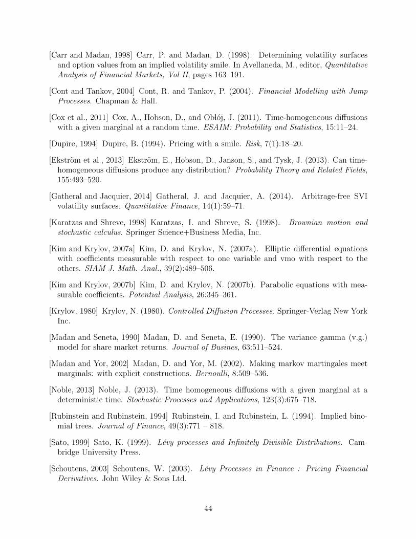
[Carr and Madan, 1998] Carr, P. and Madan, D. (1998). Determining volatility surfacesand option values from an implied volatility smile. In Avellaneda, M., editor, QuantitativeAnalysis of Financial Markets, Vol II, pages 163–191.

[Cont and Tankov, 2004] Cont, R. and Tankov, P. (2004). Financial Modelling with JumpProcesses. Chapman & Hall.

[Cox et al., 2011] Cox, A., Hobson, D., and Ob loj, J. (2011). Time-homogeneous diffusionswith a given marginal at a random time. ESAIM: Probability and Statistics, 15:11–24.

[Dupire, 1994] Dupire, B. (1994). Pricing with a smile. Risk, 7(1):18–20.

[Ekstrom et al., 2013] Ekstrom, E., Hobson, D., Janson, S., and Tysk, J. (2013). Can time-homogeneous diffusions produce any distribution? Probability Theory and Related Fields,155:493–520.

[Gatheral and Jacquier, 2014] Gatheral, J. and Jacquier, A. (2014). Arbitrage-free SVIvolatility surfaces. Quantitative Finance, 14(1):59–71.

[Karatzas and Shreve, 1998] Karatzas, I. and Shreve, S. (1998). Brownian motion andstochastic calculus. Springer Science+Business Media, Inc.

[Kim and Krylov, 2007a] Kim, D. and Krylov, N. (2007a). Elliptic differential equationswith coefficients measurable with respect to one variable and vmo with respect to theothers. SIAM J. Math. Anal., 39(2):489–506.

[Kim and Krylov, 2007b] Kim, D. and Krylov, N. (2007b). Parabolic equations with mea-surable coefficients. Potential Analysis, 26:345–361.

[Krylov, 1980] Krylov, N. (1980). Controlled Diffusion Processes. Springer-Verlag New YorkInc.

[Madan and Seneta, 1990] Madan, D. and Seneta, E. (1990). The variance gamma (v.g.)model for share market returns. Journal of Busines, 63:511–524.

[Madan and Yor, 2002] Madan, D. and Yor, M. (2002). Making markov martingales meetmarginals: with explicit constructions. Bernoulli, 8:509–536.

[Noble, 2013] Noble, J. (2013). Time homogeneous diffusions with a given marginal at adeterministic time. Stochastic Processes and Applications, 123(3):675–718.

[Rubinstein and Rubinstein, 1994] Rubinstein, I. and Rubinstein, L. (1994). Implied bino-mial trees. Journal of Finance, 49(3):771 – 818.

[Sato, 1999] Sato, K. (1999). Levy processes and Infinitely Divisible Distributions. Cam-bridge University Press.

[Schoutens, 2003] Schoutens, W. (2003). Levy Processes in Finance : Pricing FinancialDerivatives. John Wiley & Sons Ltd.

44