Embed Size (px)
Citation preview
Available online at www.sciencedirect.com
tsbwtoWldtndwacwo⃝
Kd
a
ScienceDirect
Comput. Methods Appl. Mech. Engrg. 387 (2021) 114129www.elsevier.com/locate/cma
Local extreme learning machines and domain decomposition forsolving linear and nonlinear partial differential equations
Suchuan Donga,∗, Zongwei Lib
a Center for Computational and Applied Mathematics, Department of Mathematics, Purdue University West Lafayette, IN, USAb Department of Mathematics, Purdue University, Fort Wayne, IN, USA
Received 19 December 2020; received in revised form 2 April 2021; accepted 17 June 2021Available online xxxx
Abstract
We present a neural network-based method for solving linear and nonlinear partial differential equations, by combininghe ideas of extreme learning machines (ELM), domain decomposition and local neural networks. The field solution on eachub-domain is represented by a local feed-forward neural network, and Ck continuity conditions are imposed on the sub-domainoundaries. Each local neural network consists of a small number of hidden layers, while its last hidden layer can be wide. Theeight/bias coefficients in all the hidden layers of the local neural networks are pre-set to random values and fixed throughout
he computation, and only the weight coefficients in the output layers of the local neural networks are training parameters. Theverall neural network is trained by a linear or nonlinear least squares computation, not by the back-propagation type algorithms.e introduce a block time-marching scheme together with the presented method for long-time simulations of time-dependent
inear/nonlinear partial differential equations. The current method exhibits a clear sense of convergence with respect to theegrees of freedom in the neural network. Its numerical errors typically decrease exponentially or nearly exponentially ashe number of training parameters, or the number of training data points, or the number of sub-domains increases. Extensiveumerical experiments have been performed to demonstrate the computational performance of the presented method. We alsoemonstrate its capability for long-time dynamic simulations with some test problems. We compare the presented methodith the deep Galerkin method (DGM) and the physics-informed neural network (PINN) method in terms of the accuracy
nd computational cost. The current method exhibits a clear superiority, with its numerical errors and network training timeonsiderably smaller (typically by orders of magnitude) than those of DGM and PINN. We also compare the current methodith the classical finite element method (FEM). The computational performance of the current method is on par with, andften exceeds, the FEM performance in terms of the accuracy and computational cost.c 2021 Elsevier B.V. All rights reserved.
eywords: Local extreme learning machine; Extreme learning machine; Neural network; Least squares; Nonlinear least squares; Domainecomposition
1. Introduction
Neural network based numerical methods, especially those based on deep learning [1], have attracted a significantmount of research in the past few years for simulating the governing partial differential equations (PDE) of
∗ Corresponding author.E-mail address: [email protected] (S. Dong).
https://doi.org/10.1016/j.cma.2021.1141290045-7825/ c⃝ 2021 Elsevier B.V. All rights reserved.
S. Dong and Z. Li Computer Methods in Applied Mechanics and Engineering 387 (2021) 114129
fTt1ettgwiTcPfiospo
mdsenemnTEmcato
c
physical phenomena. These methods provide a new way for approximating the field solutions, in the form ofdeep neural networks (DNN), which is different from the ansatz space with traditional numerical methods suchas finite difference or finite element techniques. This can be a promising approach, potentially more effectiveand more efficient than the traditional methods, for solving the governing PDEs of scientific and engineeringimportance. DNN-based methods solve the PDE by transforming the solution finding problem into an optimizationproblem. They typically parameterize the PDE solution by the training parameters in a deep neural network, inlight of the universal approximation property of DNNs [2–5]. Then these methods attempt to minimize a lossfunction that consists of the residual norms of the governing equations and also the associated boundary and initialconditions, typically by some flavor of gradient descent type techniques (i.e. back propagation algorithm [6,7]).This process constitutes the predominant computations in the DNN-based PDE solvers, commonly known as thetraining of the neural network. Upon convergence of the training process, the solution is represented by the neuralnetwork, with the training parameters set according to their converged values. Several successful DNN-based PDEsolvers have emerged in the past years, such as the deep Galerkin method (DGM) [8], the physics-informed neuralnetwork (PINN) [9], and related approaches (see e.g. [10–20], among others). Neural network-based PDE solutionsare smooth analytical functions, provided that smooth activation functions are used therein. The solution and itsderivatives can then be computed exactly, by evaluation of the neural network or by auto-differentiation [21].
While their computational performance is promising, DNN-based PDE solvers, in their current state, sufferrom a number of limitations that make them numerically less than satisfactory and computationally uncompetitive.he first limitation is the solution accuracy of DNN-based methods [22]. A survey of related literature indicates
hat the absolute error of the current DNN-based methods is generally on, and rarely goes below, the level of0−3∼ 10−4. Increasing the resolution or the number of training epochs/iterations does not notably improve this
rror level. The accuracy of such levels is less than satisfactory for scientific computing, especially considering thathe classical numerical methods can achieve the machine accuracy given sufficient mesh resolution and computationime. Perhaps because of such limited accuracy levels, a sense of convergence with a certain convergence rate isenerally lacking with the DNN-based PDE solvers. For example, when the number of layers, or the number of nodesithin the layers, or the number of training data points is varied systematically, one can hardly observe a consistent
mprovement in the accuracy of the obtained simulation results. Another limitation concerns the computational cost.he computational cost of DNN-based PDE solvers is extremely high. The neural network of these solvers takes aonsiderable amount of time to train, in order to reach a reasonable level of accuracy. For example, a DNN-basedDE solver can take hours to train to reach a certain accuracy, while with a traditional numerical method such as thenite element method it may take only a few seconds to produce a solution with the same or better accuracy. Becausef their limited accuracy and large computational cost, there seems to be a general sense that the DNN-based PDEolvers, at least in their current state, cannot compete with classical numerical methods, except perhaps for certainroblems such as high-dimensional PDEs which can be challenging to classical methods due to the so-called cursef dimensionality.
In the current work we concentrate on the accuracy and the computational cost of neural network-based numericalethods. We introduce a neural network-based method for solving linear and nonlinear PDEs that exhibits a
isparate computational performance from the above DNN-based PDE solvers. The current method exhibits a clearense of convergence with respect to the degrees of freedom in the system. Its numerical errors typically decreasexponentially or nearly exponentially as the number of degrees of freedom (e.g. the number of training parameters,umber of training data points) in the network increases. In terms of the accuracy and computational cost, itxhibits a clear superiority to the often-used DNN-based PDE solvers. Extensive comparisons with the deep Galerkinethod [8] and the physics-informed neural network [9] are presented in this paper. The numerical errors, and the
etwork training time, of the current method are typically orders of magnitude smaller than those of DGM and PINN.he computational performance of the current method is competitive compared with traditional numerical methods.xtensive comparisons with the classical finite element method (FEM) are provided. The performance of the currentethod is on par with, and often exceeds, the performance of FEM with regard to the accuracy and computational
ost. For example, to achieve the same accuracy, the network training time of the current method is comparable to,nd oftentimes smaller than, the FEM computation time. With the same computational cost (training/computationime), the numerical errors of the current method are comparable to, and oftentimes markedly smaller than, thosef the FEM.
The superior computational performance of the current method can be attributed to several of its algorithmicharacteristics:
2
S. Dong and Z. Li Computer Methods in Applied Mechanics and Engineering 387 (2021) 114129
• Network architecture and training parameters. The current method is based on shallow feed-forward neuralnetworks. Here “shallow” refers to the configuration that the network contains only a small number (e.g. one,two or three) of hidden layers, while the last hidden layer can be wide. The weight/bias coefficients in all thehidden layers are pre-set to random values and are fixed, and they are not training parameters. The trainingparameters consist of the weight coefficients of the output layer.• Training method. The network is trained and the values for the training parameters are determined by a least
squares computation, not by the back propagation (gradient descent-type) algorithm. For linear PDEs, trainingthe neural network involves a linear least squares computation. For nonlinear PDEs, the network traininginvolves a nonlinear least squares computation.• Domain decomposition and local neural networks. We partition the overall domain into sub-domains, and
represent the solution on each sub-domain locally by a shallow feed-forward neural network. Ck continuityconditions, where k ⩾ 0 is an integer related to the PDE order, are enforced across sub-domain boundaries.The local neural networks collectively form a multi-input multi-output logical network model, and are trainedin a coupled way with the linear or nonlinear least squares computation.• Block time marching. For long-time simulations of time-dependent PDEs, the current method adopts a block
time-marching strategy. The overall spatial–temporal domain is first divided into a number of windows intime, referred to as time blocks. The PDE is then solved on the spatial–temporal domain of each time block,individually and successively. Block time marching is crucial to long-time simulations, especially for nonlineartime-dependent PDEs.
The idea of random weight/bias coefficients in the network and the use of linear least squares method fornetwork training stem from the so-called extreme learning machines (ELM) [23,24]. ELM was developed for single-hidden layer feed-forward neural networks (SLFN), and for linear problems. It transforms the linear classificationor regression problem into a system of linear algebraic equations, which is then solved by a linear least squaresmethod or by using the pseudo-inverse (Moore–Penrose inverse) of the coefficient matrix [25]. ELM is one exampleof the so-called randomized neural networks (see e.g. [26–30]), which can be traced to Turing’s unorganizedmachine and Rosenblatt’s perceptron [31,32] and have witnessed a revival in neuro-computations in recent years.The application of ELM to function approximations and linear differential equations have been considered inseveral recent works [33–38]. Domain decomposition has found widespread applications in classical numericalmethods [39–43]. Its use in neural network-based methods, however, has been very limited and is very recent (seee.g. [22,38,44]).
The contribution of the current work lies in several aspects. A main contribution of this work is the introduction ofan ELM-like method for nonlinear differential equations, based on domain decomposition and local neural networks.In contrast, existing ELM-based methods for differential equations have been confined to linear problems, and theneural network is limited to a single hidden layer. For nonlinear problems, to solve the nonlinear system for thetraining parameters, we have adopted two methods: (i) a nonlinear least squares method with perturbations (referredto as NLSQ-perturb), and (ii) a combined Newton/linear least squares method (referred to as Newton-LLSQ). Wefind that the random perturbation in the NLSQ-perturb method is crucial to preventing the method from beingtrapped to local minima with cost values exceeding some given tolerance, especially in under-resolved cases and inlong-time simulations. We present an algorithm for effective generation of the random perturbations for the nonlinearleast squares method.
Another contribution of the current work is the aforementioned block time-marching scheme for long-timesimulations of time-dependent linear/nonlinear PDEs. When the temporal dimension of the spatial–temporal domainis large, if the PDE is solved on the entire domain all at once, we find that the neural network becomes very hard totrain with the ELM algorithm (and also with the back propagation-based algorithms), in the sense that the obtainedsolution can contain pronounced errors, especially toward later time instants in the spatial–temporal domain. On theother hand, by using the block time-marching strategy and with a moderate time block size, the problem becomesmuch easier to solve and the neural network is much easier to train with the ELM algorithm. Accurate results canbe attained with the block time-marching scheme for very long-time simulations. The block time marching strategyis often crucial to the simulations of nonlinear time-dependent PDEs when the temporal dimension becomes evenmoderately large.
We would also like to emphasize that, with the current method, each local neural network is not limited to a
single hidden layer, which is another notable difference from existing ELM-type methods. Up to three hidden layers3

S. Dong and Z. Li Computer Methods in Applied Mechanics and Engineering 387 (2021) 114129
w
ppsmtomtti
bnlsfniawdw
2
2
Ωw
wc
sbn(
ΩwkCcd
in the local neural networks have been tested in the current paper. We observe that with one or a small number(more than one) of hidden layers in the local neural networks, the current method can produce accurate simulationresults.
Since the current method is a combination of the ideas of ELM, domain decomposition, and local neural networks,e refer to this method as locELM (local extreme learning machines) in the current paper.We have performed extensive numerical experiments with linear and nonlinear, stationary and time-dependent,
artial differential equations to test the performance of the locELM method, and to study the effects of the simulationarameters involved therein. For certain test problems (e.g. the advection equation) we present very long-timeimulations to demonstrate the capability and accuracy of the locELM method together with the block time-arching scheme. We compare extensively the current locELM method with the deep Galerkin method [8] and
he physics-informed neural network method [9], and demonstrate the superiority of the current method in termsf both accuracy and the computational cost. We also compare the current method with the classical finite elementethod, and show that the computational performance of the locELM method is comparable to, and often exceeds,
he FEM performance. The current locELM method, DGM and PINN have all been implemented in Python, usinghe Tensorflow (www.tensorflow.org) and Keras (keras.io) libraries. The finite element method is also implementedn Python, by using the FEniCS library (fenicsproject.org).
The rest of this paper is structured as follows. In Section 2 we outline the locELM representation of field functionsased on domain decomposition and local extreme learning machines, and then discuss how to solve linear andonlinear differential equations using the locELM representation and how to train the overall neural network by theinear or nonlinear least squares method. We discuss the NLSQ-perturb method and the Newton-LLSQ method forolving the nonlinear differential equations. We present the block time-marching scheme, and discuss how to use itor long-time dynamic simulations. In Section 3 we present extensive numerical experiments with several linear andonlinear PDEs to test the performance of locELM. We compare locELM with DGM and PINN, and demonstratets superiority in terms of the accuracy and computational cost. We also compare locELM with the classical FEM,nd show that locELM is on par with and often outperforms the FEM. Section 4 concludes the main presentationith a number of comments on the characteristics and properties of the current method. Appendix A provides moreetails about the Newton-LLSQ method for solving nonlinear PDEs. Appendix B summarizes further locELM testsith the classical Poisson equation, and further comparisons between locELM and FEM.
. Domain decomposition and local extreme learning machines
.1. Local extreme learning machines (locELM) for representing functions
Consider the domain Ω in d (d = 1, 2 or 3) dimensions, where one of the dimensions may denote time and soin general can be a spatial–temporal domain. We consider a function f (x) (x ∈ Ω ) defined on this domain, and
ould like to represent this function using neural networks.We partition Ω into Ne (Ne ⩾ 1) non-overlapping sub-domains,
Ω = Ω1 ∪ Ω2 ∪ · · · ∪ ΩNe ,
here Ωi denotes the i th sub-domain. If Ωi and Ω j (1 ⩽ i, j ⩽ Ne) share a common boundary, we will denote thisommon boundary by Γi j .
We will represent f (x), in a spirit analogous to the finite elements or spectral elements [45–49], locally on theub-domains by local neural networks. More specifically, on each sub-domain Ωi (1 ⩽ i ⩽ Ne) we represent f (x)y a shallow feed-forward neural network [1]. Here “shallow” refers to the configuration that each local neuraletwork has only a small number (e.g. one, two or perhaps three) of hidden layers, apart from the input layerrepresenting x) and the output layer (representing f (x), restricted to Ωi ).
Let fi (x) (1 ⩽ i ⩽ Ne) denote the function f (x) restricted to Ωi . On any common boundary Γi j between Ωi andj (for all 1 ⩽ i, j ⩽ Ne), we impose the requirement that fi (x) and f j (x) satisfy the Ck continuity conditionsith an appropriate k = (k1, k2, . . . , kd ). In other words, their function values and partial derivatives up to the order
s (1 ⩽ s ⩽ d) should be continuous across the sub-domain boundary in the sth direction. The order k in thek continuity is a user-defined parameter. When solving differential equations, one can determine k for a specific
oordinate direction based on the order of the differential equation along that direction. For example, if the highest
erivative with respect to the coordinate xs (1 ⩽ s ⩽ d) involved in the equation is m, one would typically impose4

S. Dong and Z. Li Computer Methods in Applied Mechanics and Engineering 387 (2021) 114129
C
t
m−1 continuity to the solution on the sub-domain boundary along the sth direction. Thanks to these Ck continuityconditions, the local neural networks for the sub-domains, while physically separated, are coupled with one anotherlogically, and need to be trained together in a coupled fashion. The local neural networks collectively constitute therepresentation of the function f (x) on the overall domain Ω .
We impose further requirements on the local neural networks. Suppose a particular layer in the local neuralnetwork contains n nodes, and the previous layer contains m nodes. Let φi (x) (1 ⩽ i ⩽ m) denote the output ofthe previous layer, and ϕi (x) (1 ⩽ i ⩽ n) denote the output of this layer. Then the logic of this layer is representedby [1],
ϕi (x) = σ
⎛⎝ m∑j=1
φ j (x)w j i + bi
⎞⎠ , 1 ⩽ i ⩽ n, (1)
where the constants w j i and bi (1 ⩽ i ⩽ n, 1 ⩽ j ⩽ m) are the weight and bias coefficients associated with thislayer, and σ (·) is the activation function of this layer and is in general nonlinear. We assume the following for thelocal neural networks:
• The weight and bias coefficients for all the hidden layers are pre-set to uniform random values generatedon the interval [−Rm, Rm], where Rm > 0 is a user-defined constant parameter. Once these coefficientsare set randomly, they are fixed throughout the training and computation. These weight/bias coefficients arenot adjustable, and they are not training parameters of the neural network. We hereafter refer to Rm as themaximum magnitude of the random coefficients of the neural network.• The last hidden layer, i.e. the layer before the output layer, can be wide. In other words, this layer may contain
a large number of nodes. We use M to denote the number of nodes in the last hidden layer of each local neuralnetwork.• The output layer contains no bias (i.e. bi = 0) and no activation function. In other words, the output layer is
linear, i.e. σ (x) = x . The weight coefficients in the output layers of the local neural networks are adjustable.The collection of these weight coefficients constitutes the training parameters of the overall neural network.Therefore, the number of training parameters in each local neural network equals M , the number of nodes inthe last hidden layer of the local neural network.• The set of training parameters for the overall neural network is to be determined and set by a linear or nonlinear
least squares computation, not by the back propagation-type algorithm.
Remark 2.1. When a subset of the above requirements is imposed on a single global neural network, containinga single hidden layer, for the entire domain, the resultant network, when trained with a linear least squares method,is known as an extreme learning machine (ELM) [23]. In the current work we follow this terminology, and willrefer to the local neural networks presented here as local extreme learning machines (or locELM).
Let N (N ⩾ 1) denote the number of nodes in the output layer of the local neural networks. Based on the aboveassumptions, on the sub-domain Ωs (1 ⩽ s ⩽ Ne) we have the relation,
usi (x) =
M∑j=1
V sj (x)ws
ji , x ∈ Ωs, 1 ⩽ i ⩽ N , (2)
where V sj (x) (1 ⩽ j ⩽ M) denote the output of the last hidden layer, us
i (x) denote the components of outputfunction of the network, ws
ji are the training parameters on Ωs , and M denotes the number of nodes in the lasthidden layer. The function
fs(x) = (us1, us
2, . . . , usN ) (3)
is the local representation of f (x) on the sub-domain Ωs .It should be noted that the set of output functions of the last hidden layer, V s
j (x) (1 ⩽ j ⩽ M), are knownfunctions and they are fixed throughout the computation. Since the weight/bias coefficients in the hidden layersare pre-set to random values on [−Rm, Rm] and are fixed, V s
j (x) can be pre-computed by a forward evaluation ofhe local neural network (up to the last hidden layer) against the input x data. The first, second, and higher-order
s
derivatives of V j (x) with respect to the input x can then be computed by auto-differentiations.5
S. Dong and Z. Li Computer Methods in Applied Mechanics and Engineering 387 (2021) 114129
The collection of local representations fs(x) (1 ⩽ s ⩽ Ne), with Ck continuity imposed on the sub-domainboundaries and with ws
i j (1 ⩽ i ⩽ M , 1 ⩽ j ⩽ N , 1 ⩽ s ⩽ Ne) as the training parameters, form the set oftrial functions for representing the function f (x). Hereafter, we will refer to this representation as the locELMrepresentation of a function. Once the data for f (x) or the data for the governing equations that describe f (x)are given, the adjustable parameters ws
i j can be trained and determined by a linear or nonlinear least squarescomputation.
Remark 2.2. In the locELM representation, the hyper-parameters for the local neural networks associated withdifferent sub-domains (e.g. depths, widths and activation functions of the hidden layers) can in principle assumedifferent values. This can allow one to place more degrees of freedom locally in regions where the field function maybe more complicated and thus require more resolution. For simplicity of implementation, however, in the currentwork we will employ the same hyper-parameters for all the local neural networks for different sub-domains.
In the following sub-sections we focus on how to use local extreme learning machines to represent the solutionsto ordinary or partial differential equations (ODE/PDE), and discuss how to train the overall neural network byleast squares computations. We consider two cases: (i) linear differential equations, and (ii) nonlinear differentialequations, and discuss how to treat them individually. Apart from the basic algorithm, we develop a block time-marching scheme for long-time simulations of time-dependent linear/nonlinear PDEs. In the presentations we usetwo spatial dimensions, and plus time if the problem is time-dependent, as examples. The formulations can bereduced to one spatial dimension or extended to higher spatial dimensions in a straightforward fashion. For simplicitywe concentrate on rectangular spatial–temporal domains in the current work.
2.2. Linear differential equations
2.2.1. Time-independent linear differential equationsLet us first consider the boundary value problem involving linear partial differential equations together with
Dirichlet boundary conditions, and discuss how to solve the problem by using the locELM representation for thesolution. To make the discussion concrete, we concentrate on two dimensions (d = 2, with the coordinates x and y),and consider second-order partial differential equations with respect to both x and y (i.e. highest partial derivativeswith respect to x and to y are both two). The procedure outlined below can be extended to higher dimensions or tohigher-order differential equations, with appropriate boundary conditions and Ck continuity conditions taken intoaccount.
Let us consider the following generic second-order linear partial differential equation
Lu = f (x, y), (4a)
u(x, y) = g(x, y), on ∂Ω , (4b)
where L is a linear second-order operator with respect to both x and y, u(x, y) is the scalar unknown field function tobe solved for, f (x, y) and g(x, y) are prescribed source terms for the equation and the Dirichlet boundary condition,and ∂Ω denotes the boundary of Ω . We assume that this boundary value problem is well-posed. Our goal here isto illustrate the procedure for numerically solving this problem by approximating its solution using local extremelearning machines.
Here is the general idea for the solution process. We partition the overall domain into a number of sub-domains,and represent the field solution using the locELM representation described in Section 2.1. We next choose a set ofpoints (collocation points) within each sub-domain, which can have a regular or random distribution. We enforcethe governing equations on the collocation points within each sub-domain, and enforce the boundary conditions onthose collocation points in those sub-domains that reside on ∂Ω . We further enforce the Ck continuity conditions onthose collocation points that reside on the sub-domain boundaries. Auto-differentiations are employed to computethe first or higher-order derivatives involved in the above operations. These operations result in a system of algebraicequations, which may be linear or nonlinear depending on the boundary value problem, about the training parametersin the locELM representation. We seek a least squares solution to this algebraic system, and compute the solutionby either a linear least squares method or a nonlinear least squares method. The training parameters of the local
neural networks are then determined by the least squares computation.6

S. Dong and Z. Li Computer Methods in Applied Mechanics and Engineering 387 (2021) 114129
w
T
tof
RdGLiwgigrticS
For simplicity of implementation, we concentrate on the case with Ω being a rectangular domain, i.e. Ω =[a1, b1]×[a2, b2]. Let Nx (Nx ⩾ 1) and Ny (Ny ⩾ 1) denote the number of sub-domains along the x and y directions,respectively, with a total number of Ne = Nx Ny sub-domains in Ω . Let the two vectors [X0, X1, . . . , X Nx ]and [Y0, Y1, . . . , YNy ] denote the coordinates of the sub-domain boundaries along the x and y directions, where(X0, Y0) = (a1, a2) and (X Nx , YNy ) = (b1, b2). Let Ωemn = [Xm, Xm+1] × [Yn, Yn+1] denote the region occupiedby the sub-domain emn , for 0 ⩽ m ⩽ Nx − 1 and 0 ⩽ n ⩽ Ny − 1. Here emn represents the linear index of thesub-domain associated with the 2D index (m, n), with emn = m Ny + n + 1, and so 1 ⩽ emn ⩽ Ne.
We approximate the unknown field function u(x, y) using the locELM representation as discussed in Section 2.1.On each sub-domain emn we represent the solution by a shallow neural network, which consists of an input layerwith two nodes (representing the coordinates x and y), one or a small number of hidden layers, and an output layerwith one node (representing the solution uemn ). Let V emn
j (x, y) (1 ⩽ j ⩽ M) denote the output of the last hiddenlayer, where M is the number of nodes in this layer. Then Eq. (2) becomes
uemn (x, y) =M∑
j=1
V emnj (x, y)wemn
j , (x, y) ∈ Ωemn , 0 ⩽ m ⩽ Nx − 1, 0 ⩽ n ⩽ Ny − 1, (5)
here wemnj (1 ⩽ j ⩽ M) are the training parameters in the sub-domain emn . Again note that V emn
j (x, y) is known,once the weight/bias coefficients in the hidden layers have been pre-set to random values on [−Rm, Rm].
Remark 2.3. Apart from the above logical operations, in the implementation we incorporate an additionalnormalization layer immediately behind the input layer in each of the local neural networks. For each sub-domain emn , the normalization layer performs an affine mapping and normalizes the input data, (x, y) ∈ Ωemn =
[Xm, Xm+1]× [Yn, Yn+1], such that the output data of the normalization layer fall into the domain [−1, 1]× [−1, 1].his extra normalization layer contains no adjustable (training) parameters.
On the sub-domain emn (0 ⩽ m ⩽ Nx − 1, 0 ⩽ n ⩽ Ny − 1), let (xemnp , yemn
q ) (0 ⩽ p ⩽ Qx − 1, 0 ⩽ q ⩽ Q y − 1)denote a set of distinct collocation points, where xemn
p (0 ⩽ p ⩽ Qx − 1) denote a set of Qx collocation points onhe interval [Xm, Xm+1] and yemn
q denote a set of Q y collocation points on the interval [Yn, Yn+1]. The total numberf collocation points is Q = Qx Q y within each sub-domain emn . In the current work we primarily consider theollowing uniform distribution for the collocation points:
• Uniform distribution: xemnp forms a set of Qx uniform grid points on [Xm, Xm+1], with both end points included,
i.e. xemn0 = Xm and xemn
Qx−1 = Xm+1. yemnq forms a set of Q y uniform grid points on [Yn, Yn+1], with both end
points included, i.e. yemn0 = Yn and yemn
Qy−1 = Yn+1.
emark 2.4. Besides the uniform distribution, we also consider a quadrature-point distribution and a randomistribution for the collocation points. With the quadrature-point distribution, xemn
p are taken to be a set of Qx
auss–Lobatto–Legendre quadrature points on the interval [Xm, Xm+1], and yemnq are taken to be a set of Q y Gauss–
obatto–Legendre quadrature points on the interval [Yn, Yn+1]. With the random distribution, the collocation pointsn the sub-domain emn are taken to be uniformly generated random points (xemn
l , yemnl ) ∈ Ωemn (0 ⩽ l ⩽ Q − 1),
here Q is the total number of collocation points in the sub-domain, among which a certain number of points areenerated on the sub-domain boundaries and the rest are located inside the sub-domain. Numerical experimentsndicate that, with the same number of collocation points, the result with the quadrature-point distribution isenerally more accurate than that with the uniform distribution, which in turn is more accurate than that with theandom distribution of collocation points. The quadrature-point distribution however poses some practical issues inhe current implementation. When the number of quadrature points exceeds 100, the library on which the currentmplementation is based cannot compute the Gaussian quadrature points accurately. This is the reason why in theurrent work we predominantly employ the uniform distribution of collocation points in the numerical tests of
ection 3.7
S. Dong and Z. Li Computer Methods in Applied Mechanics and Engineering 387 (2021) 114129
s
w
w
it(
w
w
Rct
w
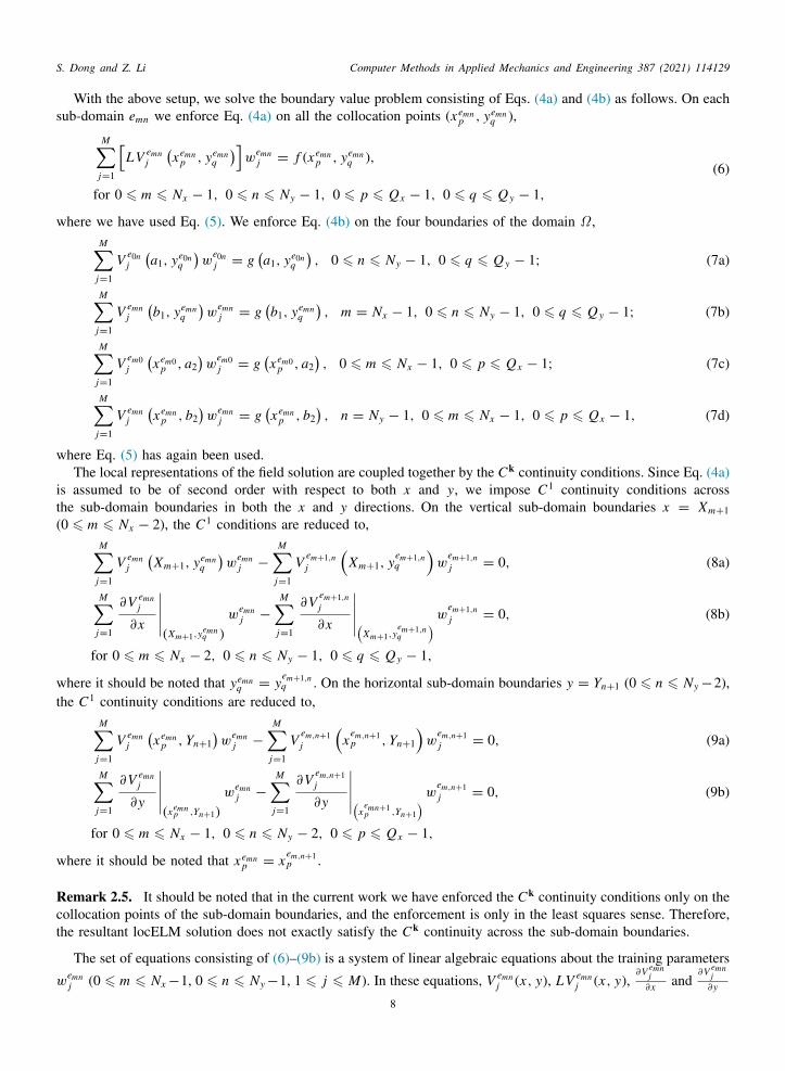
With the above setup, we solve the boundary value problem consisting of Eqs. (4a) and (4b) as follows. On eachub-domain emn we enforce Eq. (4a) on all the collocation points (xemn
p , yemnq ),
M∑j=1
[LV emn
j
(xemn
p , yemnq
)]w
emnj = f (xemn
p , yemnq ),
for 0 ⩽ m ⩽ Nx − 1, 0 ⩽ n ⩽ Ny − 1, 0 ⩽ p ⩽ Qx − 1, 0 ⩽ q ⩽ Q y − 1,
(6)
here we have used Eq. (5). We enforce Eq. (4b) on the four boundaries of the domain Ω ,M∑
j=1
V e0nj
(a1, ye0n
q
)w
e0nj = g
(a1, ye0n
q
), 0 ⩽ n ⩽ Ny − 1, 0 ⩽ q ⩽ Q y − 1; (7a)
M∑j=1
V emnj
(b1, yemn
q
)w
emnj = g
(b1, yemn
q
), m = Nx − 1, 0 ⩽ n ⩽ Ny − 1, 0 ⩽ q ⩽ Q y − 1; (7b)
M∑j=1
V em0j
(xem0
p , a2)w
em0j = g
(xem0
p , a2), 0 ⩽ m ⩽ Nx − 1, 0 ⩽ p ⩽ Qx − 1; (7c)
M∑j=1
V emnj
(xemn
p , b2)w
emnj = g
(xemn
p , b2), n = Ny − 1, 0 ⩽ m ⩽ Nx − 1, 0 ⩽ p ⩽ Qx − 1, (7d)
here Eq. (5) has again been used.The local representations of the field solution are coupled together by the Ck continuity conditions. Since Eq. (4a)
s assumed to be of second order with respect to both x and y, we impose C1 continuity conditions acrosshe sub-domain boundaries in both the x and y directions. On the vertical sub-domain boundaries x = Xm+1
0 ⩽ m ⩽ Nx − 2), the C1 conditions are reduced to,M∑
j=1
V emnj
(Xm+1, yemn
q
)w
emnj −
M∑j=1
Vem+1,nj
(Xm+1, y
em+1,nq
)w
em+1,nj = 0, (8a)
M∑j=1
∂V emnj
∂x
(Xm+1,yemn
q )
wemnj −
M∑j=1
∂Vem+1,nj
∂x
(Xm+1,y
em+1,nq
) wem+1,nj = 0, (8b)
for 0 ⩽ m ⩽ Nx − 2, 0 ⩽ n ⩽ Ny − 1, 0 ⩽ q ⩽ Q y − 1,
here it should be noted that yemnq = y
em+1,nq . On the horizontal sub-domain boundaries y = Yn+1 (0 ⩽ n ⩽ Ny−2),
the C1 continuity conditions are reduced to,M∑
j=1
V emnj
(xemn
p , Yn+1)w
emnj −
M∑j=1
Vem,n+1j
(x
em,n+1p , Yn+1
)w
em,n+1j = 0, (9a)
M∑j=1
∂V emnj
∂y
(xemn
p ,Yn+1)
wemnj −
M∑j=1
∂Vem,n+1j
∂y
(x
emn+1p ,Yn+1
) wem,n+1j = 0, (9b)
for 0 ⩽ m ⩽ Nx − 1, 0 ⩽ n ⩽ Ny − 2, 0 ⩽ p ⩽ Qx − 1,
here it should be noted that xemnp = x
em,n+1p .
emark 2.5. It should be noted that in the current work we have enforced the Ck continuity conditions only on theollocation points of the sub-domain boundaries, and the enforcement is only in the least squares sense. Therefore,he resultant locELM solution does not exactly satisfy the Ck continuity across the sub-domain boundaries.
The set of equations consisting of (6)–(9b) is a system of linear algebraic equations about the training parametersemn emn emn ∂V emn
j and∂V emn
j
j (0 ⩽ m ⩽ Nx−1, 0 ⩽ n ⩽ Ny−1, 1 ⩽ j ⩽ M). In these equations, V j (x, y), LV j (x, y),∂x ∂y
8

S. Dong and Z. Li Computer Methods in Applied Mechanics and Engineering 387 (2021) 114129
oaiwa
onK(mhA
lo
RmPfnobm
Rcpdiac
2
wci
BD
wr
are all known functions, once the weight/bias coefficients in the hidden layers are randomly set. These functions canbe evaluated on the collocation points, including those on the domain boundaries and the sub-domain boundaries.The derivatives involved in these functions can be computed by auto-differentiation.
This linear algebraic system consists of Nx Ny(Qx Q y + 2Qx + 2Q y) equations, and Nx Ny M unknown variablesf w
emnj . We seek the least squares solution to this system with the minimum norm. Linear least squares routines
re available in a number of scientific libraries, and we take advantage of these numerical libraries in ourmplementation. In the current work we employ the linear least squares routine from LAPACK, available throughrapper functions in the scipy package in Python. Therefore, the adjustable parameters w
emnj in the neural network
re trained by this linear least squares computation.In the current work we have employed Tensorflow and Keras to implement the neural network architecture as
utlined above. Each local neural network consists of several “dense” Keras layers. The set of Ne = Nx Ny localeural networks collectively forms an overall logical neural network, in the form of a multi-input multi-outputeras model. The input data to the model consist of the coordinates of the collocation points for all sub-domains,
xemnp , yemn
q ), for 0 ⩽ m ⩽ Nx − 1, 0 ⩽ n ⩽ Ny − 1, 0 ⩽ p ⩽ Qx − 1 and 0 ⩽ q ⩽ Q y − 1. The output of the Kerasodel consists of the solution uemn (x, y) on the collocation points for all the sub-domains. The output of the last
idden layer of each sub-domain, V emnj (x, y), are obtained by creating a Keras sub-model using the Keras functional
PIs (application programming interface). The derivatives of V emnj (x, y), and those involved in LV emn
j (x, y), arecomputed using auto-differentiation with these Keras sub-models. After the parameters w
emnj are obtained by the
inear least squares computation, the weight coefficients in the output layer of the Keras model are then set basedn these parameter values.
emark 2.6. We observe from numerical experiments that the simulation result obtained using the currentethod is considerably more accurate, typically by orders of magnitude, than those obtained using DNN-basedDE solvers, trained using gradient descent-type algorithms. Furthermore, the current method is computationallyast. Its computational cost is essentially the cost of the linear least squares computation. We observe that theetwork training time of the current method is considerably lower, typically by orders of magnitude, than thosef the DNN-based PDE solvers trained with gradient descent-type algorithms. These points will be demonstratedy extensive numerical experiments in Section 3, in which we compare the current method with the deep Galerkinethod [8] and the Physics-Informed Neural Network [9].
emark 2.7. The computational performance of the current locELM method, in terms of the accuracy and theomputational cost, is comparable to, and oftentimes exceeds, that of the classical finite element method. Theseoints will be demonstrated by extensive numerical experiments in Section 3 with time-independent and time-ependent problems. We observe that, with the same training/computation time, the accuracy of the current methods comparable, and oftentimes considerably superior, to that of the finite element method. To achieve the sameccuracy, the training time of the current method is comparable to, and oftentimes markedly smaller than, theomputation time of the classical finite element method.
.2.2. Time-dependent linear differential equationsWe next consider initial–boundary value problems involving time-dependent linear differential equations together
ith Dirichlet boundary conditions, and discuss how to solve such problems using the locELM method. We againoncentrate on two spatial dimensions (with coordinates x and y) plus time (t), and assume second spatial ordersn the differential equation with respect to both x and y.
asic method. We consider the following generic time-dependent second-order linear PDE, together with theirichlet boundary condition and the initial condition,
∂u∂t= Lu + f (x, y, t), (10a)
u(x, y, t) = g(x, y, t), for (x, y) on spatial domain boundary, (10b)
u(x, y, 0) = h(x, y), (10c)
here u(x, y, t) is the unknown field function to be solved for, L is a second-order linear differential operator with
espect to both x and y, f (x, y, t) is a prescribed source term, g(x, y, t) is the Dirichlet boundary data, and h(x, y)9

S. Dong and Z. Li Computer Methods in Applied Mechanics and Engineering 387 (2021) 114129
[iais(ra
lchTuidl
w
a
d[ooa
d
wd
denotes the initial field distribution. We assume that this initial–boundary value problem is well posed, and wouldlike to solve this problem by approximating u(x, y, t) using the locELM representation.
We seek the solution on a rectangular spatial–temporal domain, Ω = (x, y, t) | x ∈ [a1, b1], y ∈ [a2, b2], t ∈0,Γ ], where ai , bi (i = 1, 2) and Γ are prescribed constants. The solution procedure is analogous to that discussedn Section 2.2.1. We partition Ω into Nx (Nx ⩾ 1) sub-domains along the x direction, Ny (Ny ⩾ 1) sub-domainslong the y direction, and Nt (Nt ⩾ 1) sub-domains in time, leading to a total of Ne = Nx Ny Nt sub-domainsn Ω . Let the vectors [X0, X1, . . . , X Nx ], [Y0, Y1, . . . , YNy ] and [T0, T1, . . . , TNt ] denote the coordinates of theub-domain boundaries along the x , y and temporal directions, respectively, where (X0, Y0, T0) = (a1, a2, 0) andX Nx , YNy , TNt ) = (b1, b2,Γ ). We use Ωemnl = [Xm, Xm+1]× [Yn, Yn+1]× [Tl , Tl+1] to denote the spatial–temporalegion occupied by the sub-domain with the index emnl = m Ny Nt+nNt+l+1, for 0 ⩽ m ⩽ Nx−1, 0 ⩽ n ⩽ Ny−1nd 0 ⩽ l ⩽ Nt − 1.
We approximate u(x, y, t) using the locELM representation from Section 2.1. More specifically, we employ aocal shallow feed-forward neural network for the solution on each sub-domain emnl . The local neural networkonsists of an input layer with three nodes, representing the coordinates x , y and t , respectively, a small number ofidden layers, and an output layer consisting of one node, representing the solution uemnl (x, y, t) on this sub-domain.he output layer is linear and contains no bias. The weight/bias coefficients in all the hidden layers are pre-set toniform random values generated on [−Rm, Rm] and are fixed, as discussed in Section 2.1. Additionally, in themplementation, we incorporate an affine mapping operation right behind the input layer to normalize the inputata, (x, y, t) ∈ Ωemnl , to the interval [−1, 1]× [−1, 1]× [−1, 1]. Let V emnl
j (1 ⩽ j ⩽ M) denote the output of theast hidden layer, where M denotes the number of nodes in this layer. Then we have, in accordance with Eq. (5),
uemnl (x, y, t) =M∑
j=1
V emnlj (x, y, t)wemnl
j ,
for 0 ⩽ m ⩽ Nx − 1, 0 ⩽ n ⩽ Ny − 1, 0 ⩽ l ⩽ Nt − 1,
(11)
here the coefficients wemnlj (1 ⩽ j ⩽ M) are the training parameters of the local neural network. Note that
V emnlj (x, y, t) and its derivatives are all known functions, since the weight/bias coefficients of all the hidden layers
re pre-set and fixed.On each sub-domain emnl , let (xemnl
p , yemnlq , temnl
r ) (0 ⩽ p ⩽ Qx − 1, 0 ⩽ q ⩽ Q y − 1, and 0 ⩽ r ⩽ Qt − 1)enote a set of distinct collocation points, where xemnl
p (0 ⩽ p ⩽ Qx − 1) denotes a set of Qx collocation points onXm, Xm+1] with xemnl
0 = Xm and xemnlQx−1 = Xm+1, yemnl
q (0 ⩽ q ⩽ Q y − 1) denotes a set of Q y collocation pointsn [Yn, Yn+1] with yemnl
0 = Yn and yemnlQy−1 = Yn+1, and temnl
r (0 ⩽ r ⩽ Qt − 1) denotes a set of Qt collocation pointsn [Tl , Tl+1] with temnl
0 = Tl and temnlQt−1 = Tl+1. We primarily consider the uniform distribution of regular grid points
s the collocation points, analogous to that in Section 2.2.1.With these setup, we next enforce Eqs. (10a)–(10c) on the collocation points inside each sub-domain and on the
omain boundaries. On the sub-domain emnl , Eq. (10a) is reduced toM∑
j=1
(∂V emnl
j
∂t− LV emnl
j
)(x
emnlp ,y
emnlq ,t
emnlr )
wemnlj = f
(xemnl
p , yemnlq , temnl
r
),
for 0 ⩽ m ⩽ Nx − 1, 0 ⩽ n ⩽ Ny − 1, 0 ⩽ l ⩽ Nt − 1,
0 ⩽ p ⩽ Qx − 1, 0 ⩽ q ⩽ Q y − 1, 0 ⩽ r ⩽ Qt − 1,
(12)
here(xemnl
p , yemnlq , temnl
r)
are the collocation points. The boundary condition (10b), when enforced on the spatialomain boundaries corresponding to x = a1 or b1 and y = a2 or b2, is reduced to∑M
j=1 V e0nlj (a1, ye0nl
q , te0nlr )we0nl
j − g(a1, ye0nlq , te0nl
r ) = 0,
for 0 ⩽ n ⩽ Ny − 1, 0 ⩽ l ⩽ Nt − 1, 0 ⩽ q ⩽ Q y − 1, 0 ⩽ r ⩽ Qt − 1;(13a)∑M
j=1 V emnlj (b1, yemnl
q , temnlr )wemnl
j − g(b1, yemnlq , temnl
r ) = 0,
for m = Nx − 1, 0 ⩽ n ⩽ Ny − 1, 0 ⩽ l ⩽ Nt − 1, 0 ⩽ q ⩽ Q y − 1, 0 ⩽ r ⩽ Qt − 1;(13b)∑M
j=1 V em0lj (xem0l
p , a2, tem0lr )wem0l
j − g(xem0lp , a2, tem0l
r ) = 0, (13c)
for 0 ⩽ m ⩽ Nx − 1, 0 ⩽ l ⩽ Nt − 1, 0 ⩽ p ⩽ Qx − 1, 0 ⩽ r ⩽ Qt − 1;10

S. Dong and Z. Li Computer Methods in Applied Mechanics and Engineering 387 (2021) 114129
O
ctt
O
O
w
crln
Bnuds
∑Mj=1 V emnl
j (xemnlp , b2, temnl
r )wemnlj − g(xemnl
p , b2, temnlr ) = 0,
for n = Ny − 1, 0 ⩽ m ⩽ Nx − 1, 0 ⩽ l ⩽ Nt − 1, 0 ⩽ p ⩽ Qx − 1, 0 ⩽ r ⩽ Qt − 1.(13d)
n the boundary t = 0 of the spatial–temporal domain, the initial condition (10c) is reduced toM∑
j=1
V emn0j (xemn0
p , yemn0q , 0)wemn0
j − h(xemn0p , yemn0
q ) = 0,
for 0 ⩽ m ⩽ Nx − 1, 0 ⩽ n ⩽ Ny − 1, 0 ⩽ p ⩽ Qx − 1, 0 ⩽ q ⩽ Q y − 1.
(14)
Since L is assumed to be a second-order operator with respect to both x and y, we impose C1 continuityonditions across the sub-domain boundaries in both the x and y directions. Because Eq. (10a) is of first order inime, we impose the C0 continuity condition across the sub-domain boundaries along the temporal direction. Onhe sub-domain boundaries x = Xm+1 (0 ⩽ m ⩽ Nx − 2), the C1 conditions become,∑M
j=1 V emnlj (Xm+1, yemnl
q , temnlr )wemnl
j −∑M
j=1 Vem+1,nlj (Xm+1, y
em+1,nlq , t
em+1,nlr )w
em+1,nlj = 0,
0 ⩽ m ⩽ Nx − 2, 0 ⩽ n ⩽ Ny − 1, 0 ⩽ l ⩽ Nt − 1, 0 ⩽ q ⩽ Q y − 1, 0 ⩽ r ⩽ Qt − 1;(15a)
∑Mj=1
∂Vemnlj∂x
(Xm+1,y
emnlq ,t
emnlr )
wemnlj −
∑Mj=1
∂Vem+1,nlj∂x
(Xm+1,y
em+1,nlq ,t
em+1,nlr )
wem+1,nlj = 0,
0 ⩽ m ⩽ Nx − 2, 0 ⩽ n ⩽ Ny − 1, 0 ⩽ l ⩽ Nt − 1, 0 ⩽ q ⩽ Q y − 1, 0 ⩽ r ⩽ Qt − 1.
(15b)
n the sub-domain boundaries y = Yn+1 (0 ⩽ n ⩽ Ny − 2) the C1 continuity conditions become,∑Mj=1 V emnl
j (xemnlp , Yn+1, temnl
r )wemnlj −
∑Mj=1 V
em,n+1,lj (x
em,n+1,lp , Yn+1, t
em,n+1,lr )w
em,n+1,lj = 0,
0 ⩽ m ⩽ Nx − 1, 0 ⩽ n ⩽ Ny − 2, 0 ⩽ l ⩽ Nt − 1, 0 ⩽ p ⩽ Qx − 1, 0 ⩽ r ⩽ Qt − 1;(16a)
∑Mj=1
∂Vemnlj∂y
(x
emnlp ,Yn+1,t
emnlr )
wemnlj −
∑Mj=1
∂Vem,n+1,lj∂y
(x
em,n+1,lp ,Yn+1,t
em,n+1,lr )
wem,n+1,lj = 0,
0 ⩽ m ⩽ Nx − 1, 0 ⩽ n ⩽ Ny − 2, 0 ⩽ l ⩽ Nt − 1, 0 ⩽ p ⩽ Qx − 1, 0 ⩽ r ⩽ Qt − 1.
(16b)
n the sub-domain boundaries t = Tl+1 (0 ⩽ l ⩽ Nt − 2), the C0 continuity conditions become,M∑
j=1
V emnlj (xemnl
p , yemnlq , Tl+1)wemnl
j −
M∑j=1
Vemn,l+1j (x
emn,l+1p , y
emn,l+1q , Tl+1)w
emn,l+1j = 0,
0 ⩽ m ⩽ Nx − 1, 0 ⩽ n ⩽ Ny − 1, 0 ⩽ l ⩽ Nt − 2, 0 ⩽ p ⩽ Qx − 1, 0 ⩽ q ⩽ Q y − 1.
(17)
The equations consisting of (12)–(17) form a system of linear algebraic equations about the training parametersemnlj (1 ⩽ j ⩽ M , 0 ⩽ m ⩽ Nx − 1, 0 ⩽ n ⩽ Ny − 1 and 0 ⩽ l ⩽ Nt − 1). In these equations, V emnl
j ,∂V
emnlj∂t ,
∂Vemnlj∂x ,
∂Vemnlj∂y and LV emnl
j are all known functions and can be evaluated on the collocation points by the local neuralnetworks. In particular, the partial derivatives therein can be computed based on auto-differentiation.
This linear system consists of Nequ = Nx Ny Nt[Qx Q y Qt + 2(Qx + Q y)Qt + Qx Q y
]equations, and is about
Nx Ny Nt M unknown variables wemnlj . We seek a least squares solution to this system with minimum norm, and
ompute this solution by the linear least squares method. In the implementation we employ the linear least squaresoutine from LAPACK to compute the least squares solution. The weight coefficients in the output layers of theocal neural networks are then determined by the least squares solution to the above system. Training the neuraletwork basically consists of computing the least squares solution.
lock time-marching for long-time simulations. Since the linear least squares computation, and hence the neuraletwork training, is computationally fast, longer-time dynamic simulations of time-dependent PDEs become feasiblesing the current method. With the basic method, we observe that as the temporal dimension of the spatial–temporalomain (i.e. Γ ) increases, the network training generally becomes more difficult, in the sense that the obtainedolution tends to become less accurate corresponding to the later time instants in the domain. When Γ is large,
the solution can contain pronounced errors. Therefore, using a large dimension in time (i.e. large Γ ) with the basicmethod is generally not advisable.
To perform long-time simulations, we will employ the following block time-marching strategy. Given a spatial–temporal domain with a large dimension in time, we divide the domain into a number of windows, referred to as time
11
S. Dong and Z. Li Computer Methods in Applied Mechanics and Engineering 387 (2021) 114129
s
o
wt
T
w
N
tTbset
2
ein
2
bhp(s
t
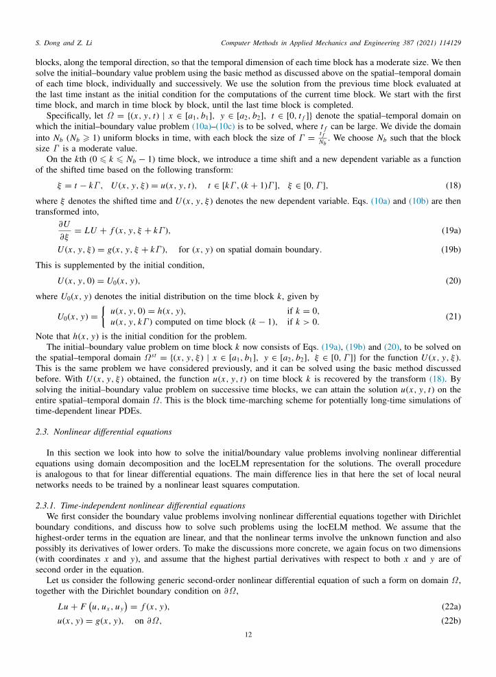
blocks, along the temporal direction, so that the temporal dimension of each time block has a moderate size. We thensolve the initial–boundary value problem using the basic method as discussed above on the spatial–temporal domainof each time block, individually and successively. We use the solution from the previous time block evaluated atthe last time instant as the initial condition for the computations of the current time block. We start with the firsttime block, and march in time block by block, until the last time block is completed.
Specifically, let Ω = (x, y, t) | x ∈ [a1, b1], y ∈ [a2, b2], t ∈ [0, t f ] denote the spatial–temporal domain onwhich the initial–boundary value problem (10a)–(10c) is to be solved, where t f can be large. We divide the domaininto Nb (Nb ⩾ 1) uniform blocks in time, with each block the size of Γ = t f
Nb. We choose Nb such that the block
ize Γ is a moderate value.On the kth (0 ⩽ k ⩽ Nb − 1) time block, we introduce a time shift and a new dependent variable as a function
f the shifted time based on the following transform:
ξ = t − kΓ , U (x, y, ξ ) = u(x, y, t), t ∈ [kΓ , (k + 1)Γ ], ξ ∈ [0,Γ ], (18)
here ξ denotes the shifted time and U (x, y, ξ ) denotes the new dependent variable. Eqs. (10a) and (10b) are thenransformed into,
∂U∂ξ= LU + f (x, y, ξ + kΓ ), (19a)
U (x, y, ξ ) = g(x, y, ξ + kΓ ), for (x, y) on spatial domain boundary. (19b)
his is supplemented by the initial condition,
U (x, y, 0) = U0(x, y), (20)
here U0(x, y) denotes the initial distribution on the time block k, given by
U0(x, y) =
u(x, y, 0) = h(x, y), if k = 0,
u(x, y, kΓ ) computed on time block (k − 1), if k > 0.(21)
ote that h(x, y) is the initial condition for the problem.The initial–boundary value problem on time block k now consists of Eqs. (19a), (19b) and (20), to be solved on
he spatial–temporal domain Ω st= (x, y, ξ ) | x ∈ [a1, b1], y ∈ [a2, b2], ξ ∈ [0,Γ ] for the function U (x, y, ξ ).
his is the same problem we have considered previously, and it can be solved using the basic method discussedefore. With U (x, y, ξ ) obtained, the function u(x, y, t) on time block k is recovered by the transform (18). Byolving the initial–boundary value problem on successive time blocks, we can attain the solution u(x, y, t) on thentire spatial–temporal domain Ω . This is the block time-marching scheme for potentially long-time simulations ofime-dependent linear PDEs.
.3. Nonlinear differential equations
In this section we look into how to solve the initial/boundary value problems involving nonlinear differentialquations using domain decomposition and the locELM representation for the solutions. The overall procedures analogous to that for linear differential equations. The main difference lies in that here the set of local neuraletworks needs to be trained by a nonlinear least squares computation.
.3.1. Time-independent nonlinear differential equationsWe first consider the boundary value problems involving nonlinear differential equations together with Dirichlet
oundary conditions, and discuss how to solve such problems using the locELM method. We assume that theighest-order terms in the equation are linear, and that the nonlinear terms involve the unknown function and alsoossibly its derivatives of lower orders. To make the discussions more concrete, we again focus on two dimensionswith coordinates x and y), and assume that the highest partial derivatives with respect to both x and y are ofecond order in the equation.
Let us consider the following generic second-order nonlinear differential equation of such a form on domain Ω ,ogether with the Dirichlet boundary condition on ∂Ω ,
Lu + F(u, ux , u y
)= f (x, y), (22a)
u(x, y) = g(x, y), on ∂Ω , (22b)12

S. Dong and Z. Li Computer Methods in Applied Mechanics and Engineering 387 (2021) 114129
idd(alLdh
o
wctCc
etn
tpc
where u(x, y) is the field function to be solved for, ux =∂u∂x , u y =
∂u∂y , L is a second-order linear differential operator
with respect to both x and y, F denotes the nonlinear term, f (x, y) is a prescribed source term, and g(x, y) denotesthe Dirichlet boundary data.
The overall procedure for solving Eqs. (22a)–(22b) using the locELM method is analogous to that in Sec-tion 2.2.1. We focus on a rectangular domain, Ω = (x, y) | x ∈ [a1, b1], y ∈ [a2, b2], and partition this domain intoNx and Ny sub-domains along the x and y directions, respectively, thus leading to a total of Ne = Nx Ny sub-domainsn Ω . Following the notation of Section 2.2.1, we denote the sub-domain boundary coordinates along the x and yirections by two vectors [X0, X1, . . . , X Nx ] and [Y0, Y1, . . . , YNy ], respectively. Let Ωemn = [Xm, Xm+1]×[Yn, Yn+1]enote the sub-domain with index emn for 0 ⩽ m ⩽ Nx − 1 and 0 ⩽ n ⩽ Ny − 1. We use (xemn
p , yemnq )
0 ⩽ p ⩽ Qx − 1, 0 ⩽ q ⩽ Q y − 1) to denote a set of uniform collocation points in the sub-domain emn , where Qxnd Q y are the number of collocation points in the x and y directions on the sub-domain. The input layer of theocal neural network consists of two nodes (x and y), and the output layer consists of one node (representing u).et uemn (x, y) denote the output of the local neural network on the sub-domain emn , and V emn
j (x, y) (1 ⩽ j ⩽ M)enote the output of the last hidden layer of the local neural network, where M is the number of nodes in the lastidden layer. We have the following relations,
uemn (x, y) =M∑
j=1
V emnj (x, y)wemn
j ,∂uemn
∂x=
M∑j=1
∂V emnj
∂xw
emnj ,
∂uemn
∂y=
M∑j=1
∂V emnj
∂yw
emnj ,
for 0 ⩽ m ⩽ Nx − 1, 0 ⩽ n ⩽ Ny − 1,
(23)
where the constants wemnj (1 ⩽ j ⩽ M) denote the weight coefficients in the output layer of the local neural network
n sub-domain emn , and they constitute the training parameters of the neural network.Enforcing Eq. (22a) on the collocation points (xemn
p , yemnq ) for each sub-domain leads to
M∑j=1
[LV emn
j (xemnp , yemn
q )]w
emnj + F
(uemn , uemn
x , uemny
)(xemn
p ,yemnq )− f (xemn
p , yemnq ) = 0,
for 0 ⩽ m ⩽ Nx − 1, 0 ⩽ n ⩽ Ny − 1, 0 ⩽ p ⩽ Qx − 1, 0 ⩽ q ⩽ Q y − 1,
(24)
here uemn , uemnx and uemn
y are given by (23) in terms of the training parameters wemnj . Enforcing the boundary
ondition (22b) on the collocation points of the four domain boundaries x = a1 or b1 and y = a2 or b2 leadso Eqs. (7a), (7b), (7c) and (7d). Since Eq. (22a) is of second-order with respect to both x and y, we impose
1 continuity conditions across the sub-domain boundaries along both the x and y directions. Enforcing the C1
ontinuity conditions on the collocation points of the sub-domain boundaries x = Xm+1 (0 ⩽ m ⩽ Nx − 2) andy = Yn+1 (0 ⩽ n ⩽ Ny − 2) leads to the Eqs. (8a)–(8b) and (9a)–(9b).
The set of equations consisting of (24), (7a)–(7d), (8a)–(8b) and (9a)–(9b) is a system of nonlinear algebraicquations about the training parameters w
emnj (1 ⩽ j ⩽ M , 0 ⩽ m ⩽ Nx − 1, 0 ⩽ n ⩽ Ny − 1). In these equations
he functions V emnj (x, y) are all known and their partial derivatives can be computed by auto-differentiation. This
onlinear algebraic system consists of Nx Ny(Qx Q y + 2Qx + 2Q y) equations with Nx Ny M unknowns.This system is to be solved for the determination of the training parameters. We seek a least squares solution
o this system for the training parameters wemnj , thus leading to a nonlinear least squares problem. To solve this
roblem, we take advantage of the nonlinear least squares implementations from the scientific libraries. In theurrent implementation, we employ the nonlinear least squares routine “least squares” from the scipy.optimize
package. This method typically works quite well, and exhibits a smooth convergence behavior. However, we observethat in certain cases, e.g. when the simulation resolution is not sufficient or sometimes in longer-time simulationswith time-dependent nonlinear equations, this method at times can be attracted to and trapped in a local minimumsolution. While the method indicates that the nonlinear iterations have converged, the norm of the converged equationresiduals can turn out to be quite pronounced in magnitude. In the event this takes place, the obtained solutioncan contain significant errors and the simulation loses accuracy from that point onward. This issue is typicallyencountered when the resolution of the computation (e.g. the number of collocation points in the domain or thenumber of training parameters in the neural network) decreases to a certain point. This has been a main issue withthe nonlinear least squares computation using this method.
To alleviate this problem and make the nonlinear least squares computation more robust, we find it necessaryto incorporate a sub-iteration procedure with random perturbations to the initial guess when invoking the nonlinear
13
S. Dong and Z. Li Computer Methods in Applied Mechanics and Engineering 387 (2021) 114129
wa
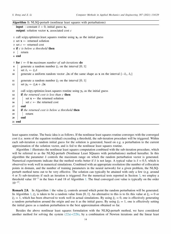
Algorithm 1: NLSQ-perturb (nonlinear least squares with perturbations)input : constant δ > 0, initial guess x0output: solution vector x, associated cost c
1 call scipy.optimize.least squares routine using x0 as the initial guess2 set x← returned solution3 set c← returned cost4 if c is below a threshold then5 return6 end
7 for i ← 0 to maximum number of sub-iterations do8 generate a random number ξ1 on the interval [0, 1]9 set δ1 ← ξ1δ
10 generate a uniform random vector ∆x of the same shape as x on the interval [−δ1, δ1]
11 generate a random number ξ2 on the interval [0, 1]12 set y0 ← ξ2x+∆x
13 call scipy.optimize.least squares routine using y0 as the initial guess14 if the returned cost is less than c then15 set x← the returned solution16 set c← the returned cost17 end18 if the returned cost is below a threshold then19 return20 end21 end
least squares routine. The basic idea is as follows. If the nonlinear least squares routine converges with the convergedcost (i.e. norm of the equation residual) exceeding a threshold, the sub-iteration procedure will be triggered. Withineach sub-iteration a random initial guess for the solution is generated, based on e.g. a perturbation to the currentapproximation of the solution vector, and is fed to the nonlinear least squares routine.
Algorithm 1 illustrates the nonlinear least squares computation combined with the sub-iteration procedure, whichill be referred to as the NLSQ-perturb (Nonlinear Least SQuares with perturbations) method hereafter. In this
lgorithm the parameter δ controls the maximum range on which the random perturbation vector is generated.Numerical experiments indicate that the method works better if δ is not large. A typical value is δ = 0.5, which isobserved to work well in numerical simulations. Combined with an appropriate resolution (the number of collocationpoints in domain, and the number of training parameters in the neural network) for a given problem, the NLSQ-perturb method turns out to be very effective. The solution can typically be attained with only a few (e.g. around4 or 5) sub-iterations if such an iteration is triggered. For the numerical tests reported in Section 3, we employ athreshold value 10−3 in the lines 4 and 18 of Algorithm 1. The final converged cost value is typically on the order10−13.
Remark 2.8. In Algorithm 1 the value ξ2 controls around which point the random perturbation will be generated.In Algorithm 1, ξ2 is taken to be a random value from [0, 1]. An alternative to this is to fix this value at ξ2 = 0 orξ2 = 1, which has been observed to work well in actual simulations. By using ξ2 = 0, one is effectively generatinga random perturbation around the origin and use it as the initial guess. By using ξ2 = 1, one is effectively settingthe initial guess as a random perturbation to the best approximation obtained so far.
Besides the above nonlinear least squares formulation with the NLSQ-perturb method, we have consideredanother method for solving the system (22a)–(22b), by a combination of Newton iterations and the linear least
14

S. Dong and Z. Li Computer Methods in Applied Mechanics and Engineering 387 (2021) 114129
csngtai
Rslu
mr
wrD
td
B[
vc0
squares approach, which we will refer to as the Newton-LLSQ (Newton-Linear Least SQuares) method hereafter.With this method, we first linearize Eq. (22a) to arrive at a linear differential equation about the increment field.This linear differential equation, the associated boundary condition, and the associated Ck continuity conditionsonstitute the system that determines the increment field. This system for the increment field is linear and can beolved using the locELM method from Section 2.2.1 with the linear least squares approach. The solution to theonlinear system consisting of (22a)–(22b) can be obtained with a Newton iteration, by starting with a zero initialuess and updating the approximation to the solution with the increment field in each Newton step. We observehat the convergence behavior of the Newton-LLSQ method is not as regular as the NLSQ-perturb method, but itppears less likely to be trapped to local minimum solutions. The details of the Newton-LLSQ method are providedn an Appendix of this paper (“Appendix A. The Newton-Linear Least Squares (Newton-LLSQ) Method”).
emark 2.9. It is observed that the computational cost of the Newton-LLSQ method is typically considerablymaller than that of the NLSQ-perturb method in training the locELM neural networks. On the other hand, theocELM solutions obtained with the Newton-LLSQ method are in general markedly less accurate than those obtainedsing the NLSQ-perturb method.
In the current work, we implement the local neural networks for each sub-domain emn using one or several denseKeras layers, with the collocation points (xemn
p , yemnq ) as the input data and uemn as the output. In the implementation,
an affine mapping is incorporated into each local neural network behind the input layer to normalize the input(x, y) data to the interval [−1, 1]× [−1, 1] for each sub-domain. The set of local neural networks logically forms a
ultiple-input multiple-output Keras model. The weight/bias coefficients in all the hidden layers are set to uniformandom values generated on [−Rm, Rm]. The weight coefficients of the output layers (wemn
j ) of the local neuralnetworks are determined and set by using the NLSQ-perturb or Newton-LLSQ methods. The partial derivativesinvolved in the formulation are computed by auto-differentiation from the Tensorflow package.
2.3.2. Time-dependent nonlinear differential equationsWe next consider the initial–boundary value problems involving time-dependent nonlinear differential equations
together with Dirichlet boundary conditions, and discuss how to solve such problems using the locELM method.We make the same assumptions about the differential equation as in Section 2.3.1: The highest-order terms areassumed to be linear, and the nonlinear terms may involve the unknown function or its partial derivatives of lowerorders. We again focus on two spatial dimensions, plus time t , and assume that the equation is of second order withrespect to both spatial coordinates (x and y).
Consider the following generic nonlinear partial differential equation of such a form on a spatial–temporal domainΩ , supplemented by the Dirichlet boundary condition and an initial condition,
∂u∂t= Lu + F(u, ux , u y)+ f (x, y, t), (25a)
u(x, y, t) = g(x, y, t), for (x, y) on the spatial domain boundary, (25b)
u(x, y, 0) = h(x, y), (25c)
here u(x, y, t) is the unknown field function to be solved for, L is a second-order linear differential operator withespect to both x and y, F denotes the nonlinear term, f (x, y, t) is a prescribed source term, g(x, y, t) denotes theirichlet boundary data, and h(x, y) is the initial field distribution.Our discussion below largely parallels that of Section 2.2.2. We first discuss the basic method on a spatial–
emporal domain, and then develop the block time-marching idea for longer-time simulations of the nonlinear partialifferential equations.
asic method. We focus on a rectangular spatial–temporal domain Ω = (x, y, t) | x ∈ [a1, b1], y ∈ [a2, b2], t ∈0,Γ ], and solve the initial–boundary value problem consisting of Eqs. (25a)–(25c) on this domain.
Following the notation of Section 2.2.2, we use Nx , Ny and Nt to denote the number of sub-domains along thex , y and t directions, where the locations of the sub-domain boundaries along the three directions are given by theectors [X0, X1, . . . , X Nx ], [Y0, Y1, . . . , YNy ] and [T0, T1, . . . , TNt ], respectively. A sub-domain with the index emnl
orresponds to the spatial–temporal region Ωemnl = [Xm, Xm+1] × [Yn, Yn+1] × [Tl , Tl+1], for 0 ⩽ m ⩽ Nx − 1,emnl emnl emnl
⩽ n ⩽ Ny − 1 and 0 ⩽ l ⩽ Nt − 1. Let (x p , yq , tr ) (0 ⩽ p ⩽ Qx − 1, 0 ⩽ q ⩽ Q y − 1, 0 ⩽ r ⩽ Qt − 1)15

S. Dong and Z. Li Computer Methods in Applied Mechanics and Engineering 387 (2021) 114129
of
waoEt
cr
ct
taS
i
Bb[t
a
w
denote the set of Q = Qx Q y Qt collocation points on each sub-domain emnl . Let uemnl (x, y, t) denote the output ofthe local neural network corresponding to the sub-domain emnl , and V emnl
j (x, y, t) (1 ⩽ j ⩽ M) denote the outputf the last hidden layer of the local neural network, where M is the number of nodes in the last hidden layer. Theollowing relations hold,⎧⎪⎪⎪⎪⎪⎪⎪⎪⎨⎪⎪⎪⎪⎪⎪⎪⎪⎩
uemnl (x, y, t) =M∑
j=1
V emnlj (x, y, t)wemnl
j , uemnlx (x, y, t) =
M∑j=1
∂V emnlj
∂xw
emnlj ,
uemnly (x, y, t) =
M∑j=1
∂V emnlj
∂yw
emnlj ,
∂uemnl
∂t=
M∑j=1
∂V emnlj
∂tw
emnlj ,
for 0 ⩽ m ⩽ Nx − 1, 0 ⩽ n ⩽ Ny − 1, 0 ⩽ l ⩽ Nt − 1,
(26)
where wemnlj denote the weight coefficients in the output layers of the local neural networks and they constitute the
training parameters of the network.Enforcing Eq. (25a) on the collocation points (xemnl
p , yemnlq , temnl
r ) of each sub-domain emnl leads to
M∑j=1
[∂V emnl
j
∂t− LV emnl
j
](x
emnlp ,y
emnlq ,t
emnlr )
wemnlj − F(uemnl , uemnl
x , uemnly )
(x
emnlp ,y
emnlq ,t
emnlr )
− f (xemnlp , yemnl
q , temnlr ) = 0,
for 0 ⩽ m ⩽ Nx − 1, 0 ⩽ n ⩽ Ny − 1, 0 ⩽ l ⩽ Nt − 1, 0 ⩽ p ⩽ Qx − 1, 0 ⩽ q ⩽ Q y − 1,
0 ⩽ r ⩽ Qt − 1,
(27)
here uemnl , uemnlx and uemnl
y are given by (26) in terms of the known function V emnlj and its partial derivatives. This is
set of nonlinear algebraic equations about the training parameters wemnlj . Enforcing the boundary condition (25b)
n the collocation points of the four spatial boundaries at x = a1 or b1 and y = a2 or b2 leads to Eqs. (13a)–(13d).nforcing the initial condition (25c) on the spatial collocation points at t = 0 results in Eq. (14). We impose
he C1 continuity conditions on the unknown field u(x, y, t) across the sub-domain boundaries along the x andy directions, since L is assumed to be a second-order operator with respect to both x and y. We impose the C0
ontinuity condition across the sub-domain boundaries in the temporal direction, since Eq. (25a) is first-order withespect to time. Enforcing the C1 continuity conditions on the collocation points on the sub-domain boundaries
x = Xm+1 (0 ⩽ m ⩽ Nx − 2) and y = Yn+1 (0 ⩽ n ⩽ Ny − 2) leads to Eqs. (15a)–(16b). Enforcing the C0
ontinuity condition on the collocation points on the sub-domain boundaries t = Tl+1 (0 ⩽ l ⩽ Nt − 2) leadso Eq. (17).
The set of equations consisting of (27) and (13a)–(17) is a nonlinear algebraic system of equations about theraining parameters w
emnlj . This system consists of Nx Ny Nt [Qx Q y Qt + 2(Qx + Q y)Qt + Qx Q y] coupled nonlinear
lgebraic equations with Nx Ny Nt M unknowns. This system can be solved using the NLSQ-perturb method fromection 2.3.1 to determine the training parameters w
emnlj .
Similarly, the system consisting of (25a)–(25c) can also be solved by the Newton-LLSQ method; see Remark A.2n Appendix A for more details.
lock time-marching. For longer-time simulations of time-dependent nonlinear differential equations, we employ alock time-marching strategy analogous to that of Section 2.2.2. Let Ω = (x, y, t)|x ∈ [a1, b1], y ∈ [a2, b2], t ∈0, t f ] denote the spatial–temporal domain on which the problem is to be solved, where t f can be large. We dividehe temporal dimension into Nb uniform time blocks, with the block size Γ =
t fNb
being a moderate value, and solvethe problem on each time block separately and successively. On the kth (0 ⩽ k ⩽ Nb−1) time block, we introduce
shifted time ξ and a new dependent variable U (x, y, ξ ) as given by Eq. (18). Then Eq. (25a) is transformed into
∂U∂ξ= LU + F(U, Ux , Uy)+ f (x, y, ξ + kΓ ), (28)
here Ux =∂U∂x and Uy =
∂U∂y . Eq. (25b) is transformed into (19b). The initial condition for time block k is given
by (20), in which the initial distribution data is given by (21).
16

S. Dong and Z. Li Computer Methods in Applied Mechanics and Engineering 387 (2021) 114129
Ω
s
c
The initial–boundary value problem consisting of Eqs. (28), (19b) and (20), on the spatial–temporal domainst= [a1, b1]× [a2, b2]× [0,Γ ], is the same problem we have considered before, and can be solved for U (x, y, ξ )
using the basic method. The solution u(x, y, t) on time block k can then be recovered by the transform (18).Starting with the first time block, we can solve the initial–boundary value problem on each time block
uccessively. After the problem on the kth block is solved, the obtained solution can be evaluated at t = (k + 1)Γand used as the initial condition for the computation on the subsequent time block.
Remark 2.10. We observe from numerical experiments that the time block size Γ can play a crucial role inlong-time simulations of time-dependent nonlinear differential equations. In general, reducing Γ can improve theconvergence of the nonlinear iterations on the time blocks. If Γ is too large, the nonlinear iterations can becomehard to converge. With the other simulation parameters (such as the number of collocation points in the time blockand the number of training parameters in the neural network) fixed, reducing the time block size effectively amountsto an increase in the resolution of the data on each time block.
Remark 2.11. We will present numerical experiments with nonlinear PDEs in Section 3 to compare the currentlocELM method with the deep Galerkin method (DGM) and the physics-informed neural network (PINN), and alsocompare the current method with the classical finite element method (FEM). We observe that for these problems thelocELM method is considerably superior to DGM and PINN, with regard to both the accuracy and the computationalcost. In terms of the computational performance, the locELM method is on par with the finite element method, andoftentimes the locELM performance exceeds the FEM performance.
3. Numerical examples
In the forthcoming section we provide a number of numerical examples to test the locELM method. Theseexamples pertain to stationary and time-dependent, linear and nonlinear differential equations. They are in generalone- or two-dimensional (1D/2D) in space, and also plus time if time-dependent. For certain problems (e.g. theadvection equation) we provide results from long-time simulations, to demonstrate the capability of the locELMmethod combined with the block time-marching scheme. We employ tanh as the activation function in all the localneural networks of this section.
We focus on the accuracy and the computational cost in our discussions. For locELM, the computational costhere refers to the total training time of the overall neural network, which includes the computation time for the
output functions of the last hidden layer and its derivatives (e.g. V emnlj ,
∂Vemnlj∂x , etc.), the computation time for the
coefficient matrix and the right hand side of the least squares problem, and the solution time for the linear/nonlinearleast squares problem. It does not include, after the training is over, the evaluation of the neural network on a set ofgiven points for the output of the solution data. The timing data is collected using the “timeit” module in Python.
We compare the current locELM method with the deep Galerkin method (DGM) [8] and the physics-informedneural network (PINN) method [9], in terms of the accuracy and the network training time. DGM and PINNare trained using both the Adam [50] and the L-BFGS [51] optimizers. For L-BFGS, we have employed theroutine available from the Tensorflow-Probability library (www.tensorflow.org/probability). For DGM and PINN,the training time refers to the time interval between the start and the end of the Adam or L-BFGS training loop fora given number of epochs/iterations. The locELM, DGM and PINN methods are all implemented in Python withthe Tensorflow (www.tensorflow.org) and Keras (keras.io) libraries.
Additionally, we compare locELM with the classical finite element method (linear elements, second-order), interms of the accuracy and computational cost. For the numerical tests reported below, the finite element method(FEM) is implemented also in Python, using the FEniCS library (fenicsproject.org). Defining the mesh, the finiteelement space, the trial and test functions, the boundary conditions, and the variational problem, as well as formingand solving the linear system, are all handled by FEniCS. In the implementation, a user only needs to specify thesecomponents symbolically; see [52]. The linear system is solved by the default linear solver in the FEniCS library,which is the sparse LU decomposition. For nonlinear differential equations, the resultant nonlinear algebraic systemis solved by the Newton’s method from the FEniCS library, with a relative tolerance 1e − 12.
When the FEM code is run for the first time, the FEniCS library uses Just-In-Time (JIT) compilers to compile
ertain key finite element operations in the Python code into C++ code, which is in turn compiled by the C++17

S. Dong and Z. Li Computer Methods in Applied Mechanics and Engineering 387 (2021) 114129
t
wvc
Wt
scdpe
(Wlnitp
pogt
pF
compiler and then cached. This is done only once. So the FEM code is slower as JIT compilation occurs whenrun for the first time, but it is much faster in subsequent runs. For FEM, the computational cost here refers tothe computation time collected using the “timeit” module after the code has been compiled by the JIT compilers.The FEM computation time includes the specifications of the mesh, the finite element space, the trial/test functionspaces, the variational problem, the forming and solution of the linear system. It does not include the output of thesolution data after the problem is solved. All the timing data with the locELM, DGM, PINN and FEM methods iscollected on a MAC computer (3.2 GHz Intel Core i5 CPU, 24GB memory) at the authors’ institution.
3.1. Helmholtz equation
In the first test we consider the boundary value problem with the one-dimensional (1D) Helmholtz equation onhe domain x ∈ [a, b],
d2udx2 − λu = f (x), (29a)
u(a) = h1, u(b) = h2, (29b)
here u(x) is the field function to be solved for, f (x) is a prescribed source term, and h1 and h2 are the boundaryalues. The other constants in the above equations and the domain specification are λ = 10, a = 0 and b = 8. Wehoose the source term f (x) such that Eq. (29a) has the following solution,
u(x) = sin(
3πx +3π
20
)cos
(2πx +
π
10
)+ 2. (30)
e choose h1 and h2 according to this analytic solution by setting x = a and x = b in (30), respectively. Underhese settings the boundary value problem (29a)–(29b) has the analytic solution (30).
We solve this problem using the locELM method presented in Section 2.2.1, by restricting the scheme to onepatial dimension. We partition [a, b] into Ne uniform sub-domains (sub-intervals), and impose the C1 continuityonditions across the sub-domain boundaries. Let Q denote the number of collocation points within each sub-omain, and consider three types of collocation points: uniform grid points, the Gauss–Lobatto–Legendre quadratureoints, and random points. The majority of tests reported below are performed with uniform collocation points inach sub-domain.
For the majority of tests in this subsection, each local neural network consists of an input layer with one noderepresenting x), an output layer with one node (representing the solution u), and one hidden layer in between.
e have also considered local neural networks with two or three hidden layers between the input and the outputayers. We employ tanh as the activation function for all the hidden layers. The output layer contains no bias ando activation function, as discussed in Section 2.1. Additionally, an affine mapping operation that normalizes thenput x data on each sub-domain to the interval [−1, 1] is incorporated into the local neural networks right behindhe input layer. This operation is implemented using the “lambda” layer in Keras, which contains no adjustablearameters and we do not count it toward the number of hidden layers. Following Section 2, let M denote the
number of nodes in the last hidden layer, which is also the number of training parameters for each sub-domain. Asdiscussed in Section 2.1, the weight and bias coefficients in the hidden layers are pre-set to uniform random valuesgenerated on the interval [−Rm, Rm] and are fixed in the computation.
The main simulation parameters with locELM include the number of sub-domains (Ne), the number of collocationpoints per sub-domain (Q), the number of training parameters per sub-domain (M), the maximum magnitude ofthe random coefficients (Rm), the number of hidden layers in the local neural network, and the type of collocationpoints in each sub-domain. We will use the total number of collocation points (Ne Q) and the total number of training
arameters (Ne M) to characterize the total degrees of freedom in the simulation. The effects of the above parametersn the simulation results will be investigated. To make the numerical tests repeatable, all the random numbers areenerated by the Tensorflow library, and we employ a fixed seed value 1 for the random number generator with allhe tests with locELM in this sub-section.
Fig. 1 illustrates the effect of the number of sub-domains in the locELM simulation, with the degrees of freedomer sub-domain (i.e. the number of collocation points and the number of training parameters per sub-domain) fixed.
igs. 1(a) and (b) show the solution and error profiles obtained with 1 sub-domain and 4 sub-domains in the locELM18
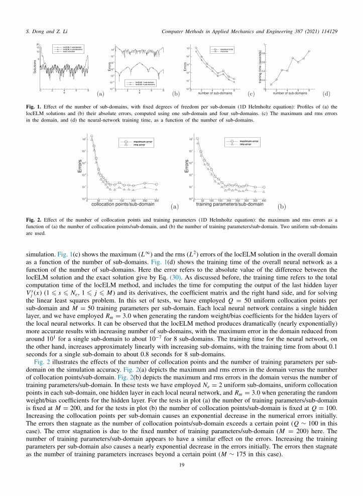
S. Dong and Z. Li Computer Methods in Applied Mechanics and Engineering 387 (2021) 114129
fa
saflc
tsltmats
dotpwiITcnpa
Fig. 1. Effect of the number of sub-domains, with fixed degrees of freedom per sub-domain (1D Helmholtz equation): Profiles of (a) thelocELM solutions and (b) their absolute errors, computed using one sub-domain and four sub-domains. (c) The maximum and rms errorsin the domain, and (d) the neural-network training time, as a function of the number of sub-domains.
Fig. 2. Effect of the number of collocation points and training parameters (1D Helmholtz equation): the maximum and rms errors as aunction of (a) the number of collocation points/sub-domain, and (b) the number of training parameters/sub-domain. Two uniform sub-domainsre used.
imulation. Fig. 1(c) shows the maximum (L∞) and the rms (L2) errors of the locELM solution in the overall domains a function of the number of sub-domains. Fig. 1(d) shows the training time of the overall neural network as aunction of the number of sub-domains. Here the error refers to the absolute value of the difference between theocELM solution and the exact solution give by Eq. (30). As discussed before, the training time refers to the totalomputation time of the locELM method, and includes the time for computing the output of the last hidden layer
V sj (x) (1 ⩽ s ⩽ Ne, 1 ⩽ j ⩽ M) and its derivatives, the coefficient matrix and the right hand side, and for solving
he linear least squares problem. In this set of tests, we have employed Q = 50 uniform collocation points perub-domain and M = 50 training parameters per sub-domain. Each local neural network contains a single hiddenayer, and we have employed Rm = 3.0 when generating the random weight/bias coefficients for the hidden layers ofhe local neural networks. It can be observed that the locELM method produces dramatically (nearly exponentially)
ore accurate results with increasing number of sub-domains, with the maximum error in the domain reduced fromround 101 for a single sub-domain to about 10−7 for 8 sub-domains. The training time for the neural network, onhe other hand, increases approximately linearly with increasing sub-domains, with the training time from about 0.1econds for a single sub-domain to about 0.8 seconds for 8 sub-domains.
Fig. 2 illustrates the effects of the number of collocation points and the number of training parameters per sub-omain on the simulation accuracy. Fig. 2(a) depicts the maximum and rms errors in the domain versus the numberf collocation points/sub-domain. Fig. 2(b) depicts the maximum and rms errors in the domain versus the number ofraining parameters/sub-domain. In these tests we have employed Ne = 2 uniform sub-domains, uniform collocationoints in each sub-domain, one hidden layer in each local neural network, and Rm = 3.0 when generating the randomeight/bias coefficients for the hidden layer. For the tests in plot (a) the number of training parameters/sub-domain
s fixed at M = 200, and for the tests in plot (b) the number of collocation points/sub-domain is fixed at Q = 100.ncreasing the collocation points per sub-domain causes an exponential decrease in the numerical errors initially.he errors then stagnate as the number of collocation points/sub-domain exceeds a certain point (Q ∼ 100 in thisase). The error stagnation is due to the fixed number of training parameters/sub-domain (M = 200) here. Theumber of training parameters/sub-domain appears to have a similar effect on the errors. Increasing the trainingarameters per sub-domain also causes a nearly exponential decrease in the errors initially. The errors then stagnates the number of training parameters increases beyond a certain point (M ∼ 175 in this case).
19
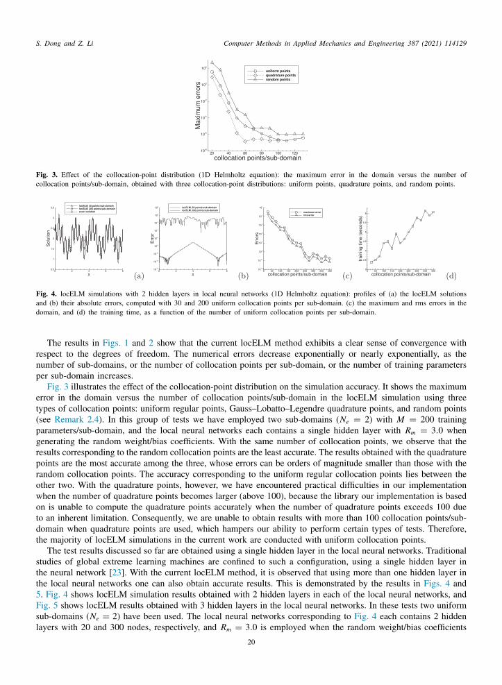
S. Dong and Z. Li Computer Methods in Applied Mechanics and Engineering 387 (2021) 114129
p
Fig. 3. Effect of the collocation-point distribution (1D Helmholtz equation): the maximum error in the domain versus the number ofcollocation points/sub-domain, obtained with three collocation-point distributions: uniform points, quadrature points, and random points.
Fig. 4. locELM simulations with 2 hidden layers in local neural networks (1D Helmholtz equation): profiles of (a) the locELM solutionsand (b) their absolute errors, computed with 30 and 200 uniform collocation points per sub-domain. (c) the maximum and rms errors in thedomain, and (d) the training time, as a function of the number of uniform collocation points per sub-domain.
The results in Figs. 1 and 2 show that the current locELM method exhibits a clear sense of convergence withrespect to the degrees of freedom. The numerical errors decrease exponentially or nearly exponentially, as thenumber of sub-domains, or the number of collocation points per sub-domain, or the number of training parametersper sub-domain increases.
Fig. 3 illustrates the effect of the collocation-point distribution on the simulation accuracy. It shows the maximumerror in the domain versus the number of collocation points/sub-domain in the locELM simulation using threetypes of collocation points: uniform regular points, Gauss–Lobatto–Legendre quadrature points, and random points(see Remark 2.4). In this group of tests we have employed two sub-domains (Ne = 2) with M = 200 training
arameters/sub-domain, and the local neural networks each contains a single hidden layer with Rm = 3.0 whengenerating the random weight/bias coefficients. With the same number of collocation points, we observe that theresults corresponding to the random collocation points are the least accurate. The results obtained with the quadraturepoints are the most accurate among the three, whose errors can be orders of magnitude smaller than those with therandom collocation points. The accuracy corresponding to the uniform regular collocation points lies between theother two. With the quadrature points, however, we have encountered practical difficulties in our implementationwhen the number of quadrature points becomes larger (above 100), because the library our implementation is basedon is unable to compute the quadrature points accurately when the number of quadrature points exceeds 100 dueto an inherent limitation. Consequently, we are unable to obtain results with more than 100 collocation points/sub-domain when quadrature points are used, which hampers our ability to perform certain types of tests. Therefore,the majority of locELM simulations in the current work are conducted with uniform collocation points.
The test results discussed so far are obtained using a single hidden layer in the local neural networks. Traditionalstudies of global extreme learning machines are confined to such a configuration, using a single hidden layer inthe neural network [23]. With the current locELM method, it is observed that using more than one hidden layer inthe local neural networks one can also obtain accurate results. This is demonstrated by the results in Figs. 4 and5. Fig. 4 shows locELM simulation results obtained with 2 hidden layers in each of the local neural networks, andFig. 5 shows locELM results obtained with 3 hidden layers in the local neural networks. In these tests two uniformsub-domains (Ne = 2) have been used. The local neural networks corresponding to Fig. 4 each contains 2 hidden
layers with 20 and 300 nodes, respectively, and Rm = 3.0 is employed when the random weight/bias coefficients20

S. Dong and Z. Li Computer Methods in Applied Mechanics and Engineering 387 (2021) 114129
gafolroelWnwloh
osn
Fig. 5. locELM simulations with 3 hidden layers in local neural networks (1D Helmholtz equation): profiles of (a) the locELM solutionsand (b) their absolute errors, computed with 30 and 200 uniform collocation points per sub-domain. (c) the maximum and rms errors in thedomain, and (d) the training time, as a function of the number of uniform collocation points per sub-domain.
for the hidden layers are generated. The local neural networks corresponding to Fig. 5 each contains 3 hidden layerswith 20, 20 and 300 nodes, respectively, and Rm = 1.0 is employed when the random weight/bias coefficients are
enerated for the hidden layers. The number of training parameters per sub-domain in these tests is therefore fixedt M = 300, which corresponds to the number of nodes in the last hidden layer. We have used tanh as the activationunction for all the hidden layers. Uniform collocation points have been used in each sub-domain, and the numberf collocation points is varied in the tests. In each of these two figures, the plots (a) and (b) are profiles of theocELM solutions and their absolute errors computed with 30 and 200 uniform collocation points per sub-domain,espectively. The plots (c) and (d) show the maximum/rms errors in the domain and the training time as a functionf the number of collocation points per sub-domain, respectively. It is evident that the numerical errors decreasexponentially with increasing collocation points/sub-domain, similar to what has been observed with a single hiddenayer from Fig. 2(a), until the errors saturate as the number of collocation points increases beyond a certain point.
ith more than one hidden layer, the locELM method can similarly produce accurate results with a sufficientumber of collocation points per sub-domain. The training time is also observed to increase essentially linearlyith respect to the number of collocation points per sub-domain. Numerical experiments with even more hidden
ayers in the local neural networks suggest that the simulation tends to be not as accurate as those corresponding tone, two or three hidden layers. It appears to be harder to obtain accurate or more accurate results with even moreidden layers.
Apart from the number of collocation points and the number of training parameters in each sub-domain, webserve that the random weight/bias coefficients in the hidden layers can influence the accuracy of the locELMimulation results. As discussed in Section 2.1, the weight/bias coefficients in the hidden layers of the localeural networks are pre-set to uniform random values generated on the interval [−Rm, Rm], and they are fixed
throughout the computation. It is observed that Rm , the maximum magnitude of the random coefficients, caninfluence significantly the simulation accuracy. Fig. 6 demonstrates this effect with two groups of tests. In the firstgroup, four uniform sub-domains (Ne = 4) are used. The number of (uniform) collocation points per sub-domain(Q) and the number of training parameters per sub-domain (M) are kept to be the same, and several of these valueshave been considered (Q = M = 50, 100, 300). Then for each of these cases we vary Rm systematically and recordthe errors of the simulation results. Fig. 6(a) shows the maximum error in the domain as a function Rm for thisgroup of tests. In the second group of tests, two uniform sub-domains (Ne = 2) are used. The number of trainingparameters per sub-domain is fixed at M = 200, and several values for the number of (uniform) collocation pointsare considered (Q = 50, 100, 200, 300). For each of these cases, Rm is varied systematically and the correspondingerrors of the simulation results are recorded. Fig. 6(b) shows the maximum error in the domain as a function ofRm for this group of tests. In both groups of tests, the local neural networks each contains a single hidden layer.These results indicate that, for a fixed simulation resolution (i.e. fixed Q and M), the error tends be worse as Rmbecomes very large or very small. The simulation tends to produce more accurate results for a range of moderateRm values, which is typically around Rm ≈ 1 ∼ 10. As the simulation resolution increases, the optimal range ofRm values tends to expand and shift rightward (toward larger values) on the Rm axis. Further tests also suggestthat with increasing number of sub-domains the optimal range of Rm values tends to shift leftward (toward smallervalues) along the Rm axis.
We observe that the use of multiple sub-domains and local extreme learning machines can significantly accelerate
the computation and reduce the network training time, without seriously compromising the accuracy, when compared21
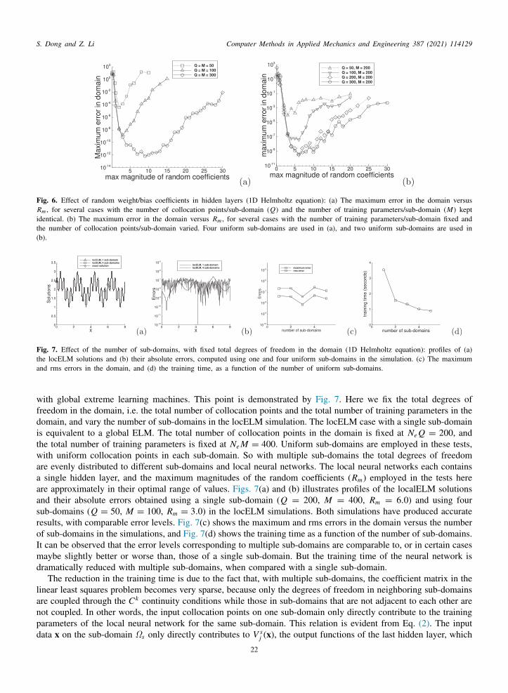
S. Dong and Z. Li Computer Methods in Applied Mechanics and Engineering 387 (2021) 114129
t(
ta
wfditwaaaasroImd
lanpd
Fig. 6. Effect of random weight/bias coefficients in hidden layers (1D Helmholtz equation): (a) The maximum error in the domain versusRm , for several cases with the number of collocation points/sub-domain (Q) and the number of training parameters/sub-domain (M) keptidentical. (b) The maximum error in the domain versus Rm , for several cases with the number of training parameters/sub-domain fixed andhe number of collocation points/sub-domain varied. Four uniform sub-domains are used in (a), and two uniform sub-domains are used inb).
Fig. 7. Effect of the number of sub-domains, with fixed total degrees of freedom in the domain (1D Helmholtz equation): profiles of (a)he locELM solutions and (b) their absolute errors, computed using one and four uniform sub-domains in the simulation. (c) The maximumnd rms errors in the domain, and (d) the training time, as a function of the number of uniform sub-domains.
ith global extreme learning machines. This point is demonstrated by Fig. 7. Here we fix the total degrees ofreedom in the domain, i.e. the total number of collocation points and the total number of training parameters in theomain, and vary the number of sub-domains in the locELM simulation. The locELM case with a single sub-domains equivalent to a global ELM. The total number of collocation points in the domain is fixed at Ne Q = 200, andhe total number of training parameters is fixed at Ne M = 400. Uniform sub-domains are employed in these tests,ith uniform collocation points in each sub-domain. So with multiple sub-domains the total degrees of freedom
re evenly distributed to different sub-domains and local neural networks. The local neural networks each containssingle hidden layer, and the maximum magnitudes of the random coefficients (Rm) employed in the tests here
re approximately in their optimal range of values. Figs. 7(a) and (b) illustrates profiles of the localELM solutionsnd their absolute errors obtained using a single sub-domain (Q = 200, M = 400, Rm = 6.0) and using fourub-domains (Q = 50, M = 100, Rm = 3.0) in the locELM simulations. Both simulations have produced accurateesults, with comparable error levels. Fig. 7(c) shows the maximum and rms errors in the domain versus the numberf sub-domains in the simulations, and Fig. 7(d) shows the training time as a function of the number of sub-domains.t can be observed that the error levels corresponding to multiple sub-domains are comparable to, or in certain casesaybe slightly better or worse than, those of a single sub-domain. But the training time of the neural network is
ramatically reduced with multiple sub-domains, when compared with a single sub-domain.The reduction in the training time is due to the fact that, with multiple sub-domains, the coefficient matrix in the
inear least squares problem becomes very sparse, because only the degrees of freedom in neighboring sub-domainsre coupled through the Ck continuity conditions while those in sub-domains that are not adjacent to each other areot coupled. In other words, the input collocation points on one sub-domain only directly contribute to the trainingarameters of the local neural network for the same sub-domain. This relation is evident from Eq. (2). The input
s
ata x on the sub-domain Ωs only directly contributes to V j (x), the output functions of the last hidden layer, which22

S. Dong and Z. Li Computer Methods in Applied Mechanics and Engineering 387 (2021) 114129
Fig. 8. Comparison between locELM, PINN and DGM (1D Helmholtz equation): profiles of (a) the solutions and (b) their absolute errors,obtained using PINN [9] and DGM [8] with the Adam and L-BFGS optimizers, and using the current locELM method.
are associated with the training parameters on the same sub-domain. Those input collocation points that reside onthe sub-domain boundaries also contribute to the training parameters of the adjacent sub-domains through the Ck
continuity conditions. In contrast, with a single global domain, all the degrees of freedom in the entire domain arecoupled with one another, and every input collocation point in the domain directly contributes to every trainingparameter in the entire neural network. This leads to a dense coefficient matrix in the linear least squares problem,and a larger time for the computation of the coefficient matrix data and the overall solution of the least squaresproblem. The above results indicate that, when compared with global ELM, the use of domain decomposition andlocal neural networks can reduce the coupling among the degrees of freedom in different sub-domains withoutseriously compromising the accuracy, and this can significantly reduce the computation time for the least squaresproblem, and hence the network training time.
We next compare the current locELM method with the physics-informed neural network (PINN) [9] method andthe deep Galerkin method (DGM) [8], two often-used PDE solvers based on deep neural networks. Fig. 8 comparesprofiles of the solutions (plot (a)) and their absolute errors (plot (b)) obtained using PINN and DGM with theAdam and the L-BFGS optimizers, and using the current locELM method. In the PINN and DGM simulations, theneural network contains 6 hidden layers with 50 nodes and the tanh activation function in each layer, and the outputlayer is linear. With PINN, the input data consist of 300 uniform collocation points in the domain. With DGM, wepartition the domain into 8 uniform sub-intervals, and employ 37 Gauss–Lobatto–Legendre quadrature points oneach sub-interval when computing the residual norm integral in the loss function. These quadrature points constitutethe input data to the neural network with DGM. In the PINN/Adam and DGM/Adam simulations, the network hasbeen trained on the input data for 45,000 epochs, with the learning rate coefficient gradually decreasing from 0.001at the beginning to 2.5×10⁻⁵ at the end. In the PINN/L-BFGS and DGM/L-BFGS simulations, the network has beentrained for 22,500 L-BFGS iterations. In the locELM simulation, four uniform sub-domains (Ne = 4) have beenused, with M = 100 training parameters per sub-domain and Q = 100 uniform collocation points per sub-domain.The four local neural networks each consists of one hidden layer with M = 100 nodes and the tanh activationfunction, and we have employed Rm = 3.0 for generating the random hidden-layer coefficients. Fig. 8 shows thatPINN, DGM and the locELM method have all captured the solution quite accurately. The error levels obtained withPINN and DGM are comparable. But the current method is considerably more accurate than PINN and DGM, bya factor of nearly five orders of magnitude in terms of the errors.
Table 1 is a further comparison of PINN, DGM and locELM in terms of the maximum/rms errors in the domain,and the computational cost (the network training time). The problem setting corresponds to that of Fig. 8. Thecurrent method is not only much more accurate than PINN and DGM, but also considerably cheaper in terms of thecomputational cost. The training time with the current locELM method is on the order of a second. In contrast, ittakes around 500 seconds to train DGM and PINN with Adam and around 1000 seconds to train them with L-BFGS.We observe a clear superiority of the locELM method to the PINN/DGM solvers in terms of both accuracy andthe computational cost. These observations will be confirmed and reinforced with other problems in subsequent
sections.23

S. Dong and Z. Li Computer Methods in Applied Mechanics and Engineering 387 (2021) 114129
tsseAuIpas
wt
Fig. 9. Comparison between locELM and FEM (1D Helmholtz equation): Profiles of (a) the solutions and (b) their absolute errors, computedusing the finite element method (FEM) and the current locELM method. (c) The maximum and rms errors in the domain versus the numberof elements from the FEM simulations, showing its second-order convergence rate.
Table 11D Helmholtz equation: Comparison between the current locELM method and PINN/DGM, interms of the maximum/rms errors in the domain, the number of epochs or iterations in the trainingof neural networks, and the training time. The problem settings correspond to those of Figs. 8.
Method Maximum error rms error Epochs/iterations Training time(seconds)
PINN (Adam) 1.06e − 3 1.57e − 4 45,000 507.7PINN (L-BFGS) 1.98e − 4 3.15e − 5 22,500 1035.8DGM (Adam) 1.57e − 3 2.98e − 4 45,000 457.0DGM (L-BFGS) 3.83e − 4 5.70e − 5 22,500 1127.7locELM 1.56e − 9 2.25e − 10 0 1.1
Table 21D Helmholtz equation: Comparison between the current locELM method and the finite element method (FEM),in terms of the maximum/rms errors in the domain and the training or computation time. The problem settingscorrespond to those of Fig. 9.
Method Elements Sub-domains Q M Maximum error rms error Wall time(seconds)
locELM – 4 100 75 4.02e − 8 5.71e − 9 0.67– 4 100 100 1.56e − 9 2.25e − 10 1.1– 4 100 125 1.42e − 10 2.55e − 11 1.3
FEM 25,000 – – – 6.82e − 8 1.74e − 8 0.3250,000 – – – 1.67e − 8 4.35e − 9 0.62100,000 – – – 1.33e − 8 3.30e − 9 1.24
Finally we compare the current locELM method with the classical finite element method (FEM). We observe thathe computational performance of locELM is comparable to that of FEM, and oftentimes the locELM performanceurpasses that of FEM, in terms of the accuracy and computational cost. Figs. 9(a) and (b) are comparisons of theolution profiles and the error profiles obtained using locELM and FEM. Fig. 9(c) shows the maximum and rmsrrors as a function of the number of elements obtained using FEM, demonstrating its second-order convergence rate.s mentioned before, the finite element method is implemented in Python using the FEniCS library. In these testsniform linear elements have been used. For the plots (a) and (b), 100,000 elements are used in the FEM simulation.n the locELM simulation, we have employed Ne = 4 uniform sub-domains, Q = 100 uniform collocation pointser sub-domain, M = 100 training parameters per sub-domain, a single hidden layer in the local neural networks,nd Rm = 3.0 when generating the random coefficients. It is evident that both FEM and locELM produce accurateolutions.
Table 2 provides a more comprehensive comparison between locELM and FEM for the 1D Helmholtz equation,ith regard to the accuracy and computational cost. Here we list the maximum and rms errors in the domain, and
he training or computation time, obtained using locELM and FEM corresponding to several numerical resolutions.
24
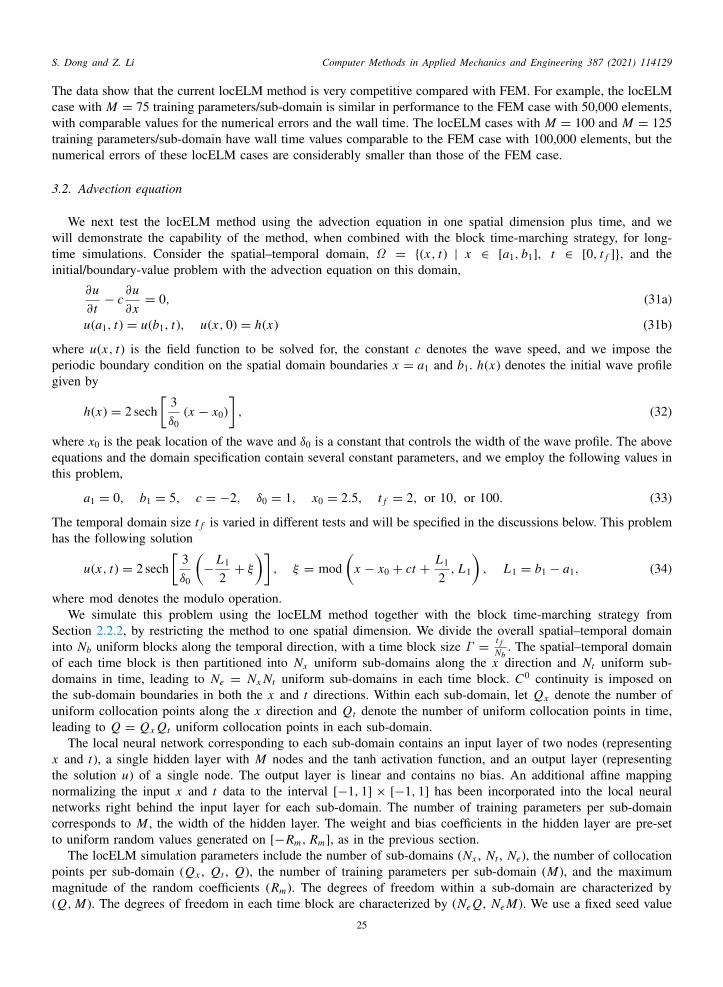
S. Dong and Z. Li Computer Methods in Applied Mechanics and Engineering 387 (2021) 114129
tn
3
wti
g
Th
w
Si
tnnct
m(
The data show that the current locELM method is very competitive compared with FEM. For example, the locELMcase with M = 75 training parameters/sub-domain is similar in performance to the FEM case with 50,000 elements,with comparable values for the numerical errors and the wall time. The locELM cases with M = 100 and M = 125raining parameters/sub-domain have wall time values comparable to the FEM case with 100,000 elements, but theumerical errors of these locELM cases are considerably smaller than those of the FEM case.
.2. Advection equation
We next test the locELM method using the advection equation in one spatial dimension plus time, and weill demonstrate the capability of the method, when combined with the block time-marching strategy, for long-
ime simulations. Consider the spatial–temporal domain, Ω = (x, t) | x ∈ [a1, b1], t ∈ [0, t f ], and thenitial/boundary-value problem with the advection equation on this domain,
∂u∂t− c
∂u∂x= 0, (31a)
u(a1, t) = u(b1, t), u(x, 0) = h(x) (31b)
where u(x, t) is the field function to be solved for, the constant c denotes the wave speed, and we impose theperiodic boundary condition on the spatial domain boundaries x = a1 and b1. h(x) denotes the initial wave profile
iven by
h(x) = 2 sech[
3δ0
(x − x0)
], (32)
where x0 is the peak location of the wave and δ0 is a constant that controls the width of the wave profile. The aboveequations and the domain specification contain several constant parameters, and we employ the following values inthis problem,
a1 = 0, b1 = 5, c = −2, δ0 = 1, x0 = 2.5, t f = 2, or 10, or 100. (33)
he temporal domain size t f is varied in different tests and will be specified in the discussions below. This problemas the following solution
u(x, t) = 2 sech[
3δ0
(−
L1
2+ ξ
)], ξ = mod
(x − x0 + ct +
L1
2, L1
), L1 = b1 − a1, (34)
here mod denotes the modulo operation.We simulate this problem using the locELM method together with the block time-marching strategy from
ection 2.2.2, by restricting the method to one spatial dimension. We divide the overall spatial–temporal domainnto Nb uniform blocks along the temporal direction, with a time block size Γ =
t fNb
. The spatial–temporal domainof each time block is then partitioned into Nx uniform sub-domains along the x direction and Nt uniform sub-domains in time, leading to Ne = Nx Nt uniform sub-domains in each time block. C0 continuity is imposed onthe sub-domain boundaries in both the x and t directions. Within each sub-domain, let Qx denote the number ofuniform collocation points along the x direction and Qt denote the number of uniform collocation points in time,leading to Q = Qx Qt uniform collocation points in each sub-domain.
The local neural network corresponding to each sub-domain contains an input layer of two nodes (representingx and t), a single hidden layer with M nodes and the tanh activation function, and an output layer (representinghe solution u) of a single node. The output layer is linear and contains no bias. An additional affine mappingormalizing the input x and t data to the interval [−1, 1] × [−1, 1] has been incorporated into the local neuraletworks right behind the input layer for each sub-domain. The number of training parameters per sub-domainorresponds to M , the width of the hidden layer. The weight and bias coefficients in the hidden layer are pre-seto uniform random values generated on [−Rm, Rm], as in the previous section.
The locELM simulation parameters include the number of sub-domains (Nx , Nt , Ne), the number of collocationpoints per sub-domain (Qx , Qt , Q), the number of training parameters per sub-domain (M), and the maximum
agnitude of the random coefficients (Rm). The degrees of freedom within a sub-domain are characterized by
Q, M). The degrees of freedom in each time block are characterized by (Ne Q, Ne M). We use a fixed seed value25

S. Dong and Z. Li Computer Methods in Applied Mechanics and Engineering 387 (2021) 114129
d
npfi
1n
swuir
thtfWndbas
o
Fig. 10. Advection equation: Distributions of (a) the locELM solution and (b) its absolute error in the spatial–temporal plane. The temporalomain size is t f = 10, and 10 time blocks are used in the simulation.
Fig. 11. Effect of the degrees of freedom (advection equation): the maximum and rms errors in the overall domain as a function of (a) theumber of sub-domains, (b) the number of collocation points in each direction per sub-domain, and (c) the number of training parameterser sub-domain. Temporal domain size is t f = 10, and 10 time blocks have been used. In (a), the degrees of freedom per sub-domain arexed. In (b) and (c), Ne = 8 sub-domains per time block are used.
for the Tensorflow random number generators in all the tests with locELM of this sub-section, so that all theumerical tests here are repeatable.
Fig. 10 illustrates the solution from the locELM simulation. Plotted here are the distributions of the locELMolution and its absolute error in the spatial–temporal plane. In this test, the temporal domain size is t f = 10, ande employ 10 uniform time blocks (Nb = 10) in this domain. Within each time block, we have employed Ne = 8niform sub-domains (with Nx = 4 and Nt = 2), and Q = 20 × 20 uniform collocation points (Qx = Qt = 20)n each sub-domain. We employ M = 300 training parameters per sub-domain, and Rm = 1.0 when generating theandom weight/bias coefficients. It is evident that the current method has captured the wave solution accurately.
The effect of the degrees of freedom on the simulation accuracy is illustrated by Fig. 11. In this group of tests, theemporal domain size is fixed at t f = 10. We have employed Nb = 10 uniform time blocks within the domain, oneidden layer in each local neural network, and Rm = 1.0 when generating the random weight/bias coefficients forhe hidden layers. Fig. 11(a) illustrates the effect of the number of sub-domains per time block, when the degrees ofreedom per sub-domain are fixed. Here the number of sub-domains within each time block is varied systematically.
e employ a fixed set of Q = 20 × 20 uniform collocation points per sub-domain (Qx = Qt = 20), and fix theumber of training parameters per sub-domain at M = 300. This plot shows the maximum and rms errors in theomain as a function of the number of sub-domains per time block. Here the case with Ne = 2 sub-domains/time-lock corresponds to (Nx , Nt ) = (2, 1). The case with Ne = 4 sub-domains corresponds to (Nx , Nt ) = (2, 2),nd the case with Ne = 8 sub-domains corresponds to (Nx , Nt ) = (4, 2). It can be observed that, with increasingub-domains/time-block, the rate of reduction in the errors, while not very regular, is approximately exponential.
Fig. 11(b) shows the maximum and rms errors in the entire spatial–temporal domain as a function of the number
f collocation points in each direction (with Qx = Qt maintained) in each sub-domain. Fig. 11(c) shows the26

S. Dong and Z. Li Computer Methods in Applied Mechanics and Engineering 387 (2021) 114129
p
n
cht
Fig. 12. Effect of the random coefficients (advection equation): the maximum and rms errors in the domain as a function of Rm , themaximum magnitude of the random coefficients in hidden layer of local neural networks.
Fig. 13. Long-time simulation of the advection equation: distributions of (a) the locELM solution and (b) its absolute error in thespatial–temporal plane for a long-time simulation. In these tests 100 time blocks in the domain and 8 sub-domains per time block areused.
maximum and rms errors in the entire domain as a function of the number of training parameters per sub-domain.In these tests, we have employed 8 sub-domains (Nx = 4, Nt = 2) per time block. For those tests of Fig. 11(b), thenumber of training parameters/sub-domain is fixed at M = 300. For the tests of Fig. 11(c), the number of collocation
oints/sub-domains is fixed at Q = 20 × 20 (Qx = Qt = 20). With the increase of the collocation points in eachdirection, or the increase of the training parameters per sub-domain, we can observe an approximately exponentialdecrease in the maximum and rms errors. When the number of collocation points (or training parameters) increasesabove a certain point, the errors start to stagnate, apparently because of the fixed number of training parameters (orthe fixed number of collocation points) in these tests. The sense of convergence exhibited by the current locELMmethod is unmistakable.
The effect of the random coefficients in the hidden layers of the local neural networks on the simulation accuracyis illustrated in Fig. 12. This plot shows the maximum and rms errors in the domain as a function of Rm , themaximum magnitude of the random weight/bias coefficients. In this set of experiments, the temporal domain sizeis t f = 10, and Nb = 10 time blocks are used in the domain. We have employed 8 uniform sub-domains pertime block (Nx = 4, Nt = 2), Q = 20 × 20 uniform collocation points per sub-domain (Qx = Qt = 20), andM = 300 training parameters per sub-domain. The weight/bias coefficients in the hidden layers of the local neuraletworks are set to uniform random values generated on [−Rm, Rm], and Rm is varied systematically in these tests.
Very large or very small values of Rm have an adverse effect on the simulation accuracy. Better accuracy generallycorresponds to a range of moderate Rm values.
Thanks to its accuracy and favorable computational cost, it is feasible to perform long-time simulations of time-dependent PDEs using the current locELM method. Figs. 13 and 14 demonstrate a long-time simulation of theadvection equation with the current method. In this simulation, the temporal domain size is set to t f = 100, whichamounts to approximately 40 periods of the wave propagation time. In the simulation we have employed 100 uniformtime blocks in the domain, 8 uniform sub-domains per time block (with Nx = 4 and Nt = 2), 20 × 20 uniformollocation points per sub-domain (i.e. Qx = Qt = 20), 300 training parameters per sub-domain (M = 300), a singleidden layer in each local neural network, and Rm = 1.0 when generating the random weight/bias coefficients for
he hidden layers of the local neural networks. The total network training time for this locELM computation is about27
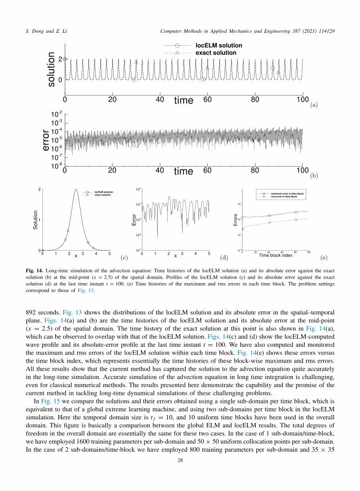
S. Dong and Z. Li Computer Methods in Applied Mechanics and Engineering 387 (2021) 114129
ssc
8p(wwttAiec
esdfwI
Fig. 14. Long-time simulation of the advection equation: Time histories of the locELM solution (a) and its absolute error against the exactolution (b) at the mid-point (x = 2.5) of the spatial domain. Profiles of the locELM solution (c) and its absolute error against the exactolution (d) at the last time instant t = 100. (e) Time histories of the maximum and rms errors in each time block. The problem settingsorrespond to those of Fig. 13.
92 seconds. Fig. 13 shows the distributions of the locELM solution and its absolute error in the spatial–temporallane. Figs. 14(a) and (b) are the time histories of the locELM solution and its absolute error at the mid-pointx = 2.5) of the spatial domain. The time history of the exact solution at this point is also shown in Fig. 14(a),hich can be observed to overlap with that of the locELM solution. Figs. 14(c) and (d) show the locELM-computedave profile and its absolute-error profile at the last time instant t = 100. We have also computed and monitored
he maximum and rms errors of the locELM solution within each time block. Fig. 14(e) shows these errors versushe time block index, which represents essentially the time histories of these block-wise maximum and rms errors.ll these results show that the current method has captured the solution to the advection equation quite accurately
n the long-time simulation. Accurate simulation of the advection equation in long time integration is challenging,ven for classical numerical methods. The results presented here demonstrate the capability and the promise of theurrent method in tackling long-time dynamical simulations of these challenging problems.
In Fig. 15 we compare the solutions and their errors obtained using a single sub-domain per time block, which isquivalent to that of a global extreme learning machine, and using two sub-domains per time block in the locELMimulation. Here the temporal domain size is t f = 10, and 10 uniform time blocks have been used in the overallomain. This figure is basically a comparison between the global ELM and locELM results. The total degrees ofreedom in the overall domain are essentially the same for these two cases. In the case of 1 sub-domain/time-block,e have employed 1600 training parameters per sub-domain and 50× 50 uniform collocation points per sub-domain.
n the case of 2 sub-domains/time-block we have employed 800 training parameters per sub-domain and 35 × 35
28
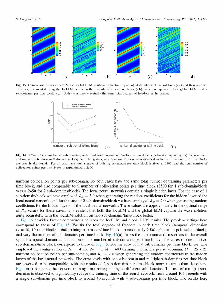
S. Dong and Z. Li Computer Methods in Applied Mechanics and Engineering 387 (2021) 114129
aac
utvslcoq
ctasseulaFda
Fig. 15. Comparison between locELM and global ELM solutions (advection equation): distributions of the solutions (a,c) and their absoluteerrors (b,d) computed using the locELM method with 1 sub-domain per time block (a,b), which is equivalent to a global ELM, and 2sub-domains per time block (c,d). Both cases have essentially the same total degrees of freedom in the domain.
Fig. 16. Effect of the number of sub-domains, with fixed total degrees of freedom in the domain (advection equation): (a) the maximumnd rms errors in the overall domain, and (b) the training time, as a function of the number of sub-domains per time-block. 10 time blocksre used in the domain. For all cases, the total number of training parameters per time block is fixed at 1600, and the total number ofollocation points per time block is approximately 2500.
niform collocation points per sub-domain. So both cases have the same total number of training parameters perime block, and also comparable total number of collocation points per time block (2500 for 1 sub-domain/blockersus 2450 for 2 sub-domains/block). The local neural networks contain a single hidden layer. For the case of 1ub-domain/block we have employed Rm = 3.0 when generating the random coefficients for the hidden layer of theocal neural network, and for the case of 2 sub-domains/block we have employed Rm = 2.0 when generating randomoefficients for the hidden layers of the local neural networks. These values are approximately in the optimal rangef Rm values for these cases. It is evident that both the locELM and the global ELM capture the wave solutionuite accurately, with the locELM solution on two sub-domains/time-block better.
Fig. 16 provides further comparisons between the locELM and global ELM results. The problem settings hereorrespond to those of Fig. 15. We fix the total degrees of freedom in each time block (temporal dimensionf = 10, 10 time blocks, 1600 training parameters/time-block, approximately 2500 collocation points/time-block),nd vary the number of sub-domains per time block. Fig. 16(a) shows the maximum and rms errors in the overallpatial–temporal domain as a function of the number of sub-domains per time block. The cases of one and twoub-domains/time-block correspond to those of Fig. 15. For the case with 4 sub-domains per time-block, we havemployed the configuration of Nx = 4 and Nt = 1, M = 400 training parameters per sub-domain, Q = 25 × 25niform collocation points per sub-domain, and Rm = 2.0 when generating the random coefficients in the hiddenayers of the local neural networks. The error levels with one sub-domain and multiple sub-domains per time blockre observed to be comparable, with the results of 2 sub-domains per time block more accurate than the others.ig. 16(b) compares the network training time corresponding to different sub-domains. The use of multiple sub-omains is observed to significantly reduce the training time of the neural network, from around 105 seconds with
single sub-domain per time block to around 40 seconds with 4 sub-domains per time block. The results here29
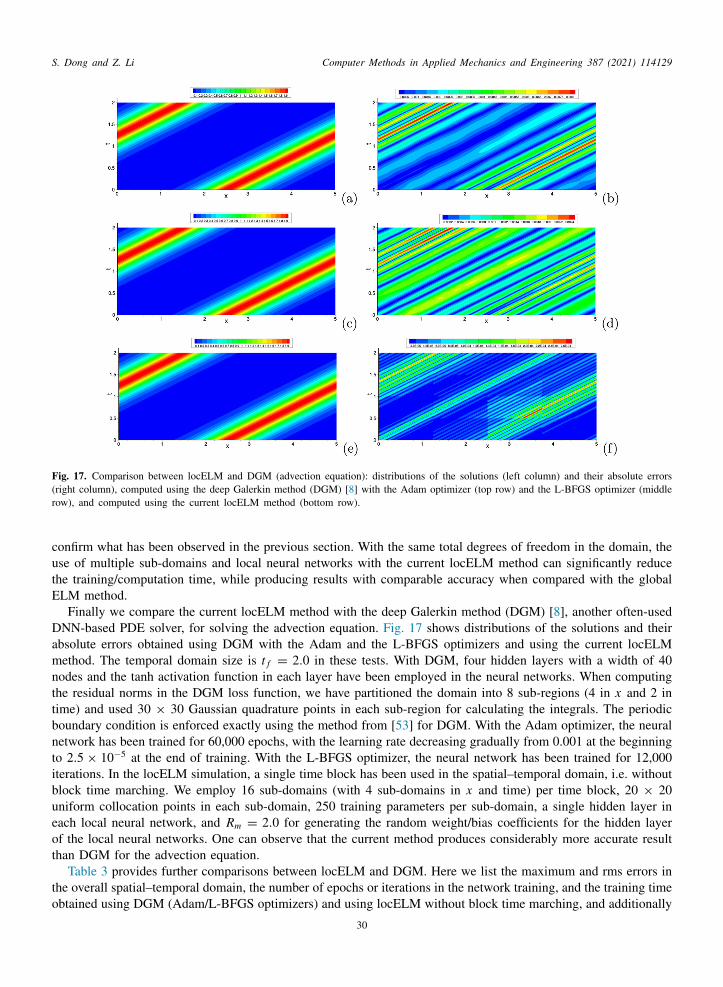
S. Dong and Z. Li Computer Methods in Applied Mechanics and Engineering 387 (2021) 114129
(r
cutE
Dam
bntib
Fig. 17. Comparison between locELM and DGM (advection equation): distributions of the solutions (left column) and their absolute errorsright column), computed using the deep Galerkin method (DGM) [8] with the Adam optimizer (top row) and the L-BFGS optimizer (middleow), and computed using the current locELM method (bottom row).
onfirm what has been observed in the previous section. With the same total degrees of freedom in the domain, these of multiple sub-domains and local neural networks with the current locELM method can significantly reducehe training/computation time, while producing results with comparable accuracy when compared with the globalLM method.
Finally we compare the current locELM method with the deep Galerkin method (DGM) [8], another often-usedNN-based PDE solver, for solving the advection equation. Fig. 17 shows distributions of the solutions and their
bsolute errors obtained using DGM with the Adam and the L-BFGS optimizers and using the current locELMethod. The temporal domain size is t f = 2.0 in these tests. With DGM, four hidden layers with a width of 40
nodes and the tanh activation function in each layer have been employed in the neural networks. When computingthe residual norms in the DGM loss function, we have partitioned the domain into 8 sub-regions (4 in x and 2 intime) and used 30 × 30 Gaussian quadrature points in each sub-region for calculating the integrals. The periodic
oundary condition is enforced exactly using the method from [53] for DGM. With the Adam optimizer, the neuraletwork has been trained for 60,000 epochs, with the learning rate decreasing gradually from 0.001 at the beginningo 2.5 × 10⁻⁵ at the end of training. With the L-BFGS optimizer, the neural network has been trained for 12,000terations. In the locELM simulation, a single time block has been used in the spatial–temporal domain, i.e. withoutlock time marching. We employ 16 sub-domains (with 4 sub-domains in x and time) per time block, 20 × 20
uniform collocation points in each sub-domain, 250 training parameters per sub-domain, a single hidden layer ineach local neural network, and Rm = 2.0 for generating the random weight/bias coefficients for the hidden layerof the local neural networks. One can observe that the current method produces considerably more accurate resultthan DGM for the advection equation.
Table 3 provides further comparisons between locELM and DGM. Here we list the maximum and rms errors inthe overall spatial–temporal domain, the number of epochs or iterations in the network training, and the training time
obtained using DGM (Adam/L-BFGS optimizers) and using locELM without block time marching, and additionally30
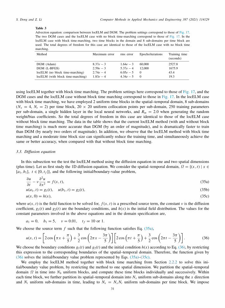
S. Dong and Z. Li Computer Methods in Applied Mechanics and Engineering 387 (2021) 114129
Wt(
tdea
Table 3Advection equation: comparison between locELM and DGM. The problem settings correspond to those of Fig. 17.The two DGM cases and the locELM case with no block time-marching correspond to those of Fig. 17. In thelocELM case with block time-marching, two time blocks in the domain and 8 sub-domains per time block areused. The total degrees of freedom for this case are identical to those of the locELM case with no block timemarching.
Method Maximum error rms error Epochs/iterations Training time(seconds)
DGM (Adam) 8.37e − 3 1.64e − 3 60,000 2527.8DGM (L-BFGS) 2.59e − 3 5.37e − 4 12,000 1675.9locELM (no block time-marching) 2.74e − 4 6.05e − 5 0 43.4locELM (with block time-marching) 1.83e − 4 4.34e − 5 0 19.3
using locELM together with block time marching. The problem settings here correspond to those of Fig. 17, and theDGM cases and the locELM case without block time marching correspond to those in Fig. 17. In the locELM casewith block time marching, we have employed 2 uniform time blocks in the spatial–temporal domain, 8 sub-domains(Nx = 4, Nt = 2) per time block, 20 × 20 uniform collocation points per sub-domain, 250 training parametersper sub-domain, a single hidden layer in the local neural networks, and Rm = 2.0 when generating the randomweight/bias coefficients. So the total degrees of freedom in this case are identical to those of the locELM casewithout block time marching. The data in the table shows that the current locELM method (with and without blocktime marching) is much more accurate than DGM (by an order of magnitude), and is dramatically faster to trainthan DGM (by nearly two orders of magnitude). In addition, we observe that the locELM method with block timemarching and a moderate time block size can significantly reduce the training time, and simultaneously achieve thesame or better accuracy, when compared with that without block time marching.
3.3. Diffusion equation
In this subsection we the test the locELM method using the diffusion equation in one and two spatial dimensions(plus time). Let us first study the 1D diffusion equation. We consider the spatial–temporal domain, Ω = (x, t) | x ∈[a1, b1], t ∈ [0, t f ], and the following initial/boundary-value problem,
∂u∂t− ν
∂2u∂x2 = f (x, t), (35a)
u(a1, t) = g1(t), u(b1, t) = g2(t), (35b)
u(x, 0) = h(x), (35c)
where u(x, t) is the field function to be solved for, f (x, t) is a prescribed source term, the constant ν is the diffusioncoefficient, g1(t) and g2(t) are the boundary conditions, and h(x) is the initial field distribution. The values for theconstant parameters involved in the above equations and in the domain specification are,
a1 = 0, b1 = 5, ν = 0.01, t f = 10 or 1.
We choose the source term f such that the following function satisfies Eq. (35a),
u(x, t) =[
2 cos(πx +
π
5
)+
32
cos(
2πx −3π
5
)][2 cos
(π t +
π
5
)+
32
cos(
2π t −3π
5
)]. (36)
e choose the boundary conditions g1(t) and g2(t) and the initial condition h(x) according to Eq. (36), by restrictinghis expression to the corresponding boundaries of the spatial–temporal domain. Therefore, the function given by36) solves the initial/boundary value problem represented by Eqs. (35a)–(35c).
We employ the locELM method together with block time marching from Section 2.2.2 to solve this ini-ial/boundary value problem, by restricting the method to one spatial dimension. We partition the spatial–temporalomain Ω in time into Nb uniform blocks, and compute these time blocks individually and successively. Withinach time block, we further partition its spatial–temporal domain into Nx uniform sub-domains along the x directionnd N uniform sub-domains in time, leading to N = N N uniform sub-domains per time block. We impose
t e x t31

S. Dong and Z. Li Computer Methods in Applied Mechanics and Engineering 387 (2021) 114129
Cbdu
ltaorwni[i
tppt
t
itot
tdfot
p
Fig. 18. 1D diffusion equation: distributions of the solution (a) and its absolute error (b) computed using the current locELM method. 10time blocks and 5 sub-domains per time block are employed.
1 continuity conditions on the sub-domain boundaries in the x direction and C0 continuity on the sub-domainoundaries in the temporal direction. Within each sub-domain we use Qx uniform collocation points along the xirection and Qt uniform collocation points in time as the input training data, leading to a total of Q = Qx Qt
niform collocation points per sub-domain.We use one local neural network to approximate the solution on each sub-domain within the time block, thus
eading to a total of Ne local neural networks in the locELM simulation. In the majority of tests of this subsectionhe local neural networks each contains a single hidden layer with M nodes and the tanh activation function. Welso report results obtained with the local neural networks containing more than one hidden layer. The input layerf the local neural networks consists of two nodes, representing x and t . The output layer consists of a single node,epresenting the solution u, and has no bias coefficient and no activation function. As in previous subsections,e incorporate an additional affine mapping operation right behind the input layer of the local neural network toormalize the input x and t data to the interval [−1, 1]× [−1, 1] in each sub-domain. The weight/bias coefficientsn the hidden layer of each of the local neural networks are set to uniform random values generated on the interval−Rm, Rm]. We use a fixed seed value 22 for the Tensorflow random number generator for all the tests with locELMn this subsection.
The locELM simulation parameters include the number of time blocks (Nb), the number of sub-domains perime block (Ne, Nx , Nt ), the number of training parameters per sub-domain (M), the number of collocation pointser sub-domain (Qx , Qt , Q), and the maximum magnitude of the random coefficients (Rm). In accordance withrevious subsections, we use (Q, M) to characterize the degrees of freedom within a sub-domain, and (Ne Q, Ne M)o characterize the degrees of freedom within a time block.
Fig. 18 shows distributions of the locELM solution and its absolute error in the spatial–temporal plane. In thisest the temporal domain size is set to t f = 10. We have employed Nb = 10 uniform time blocks in the simulation,Ne = 5 uniform sub-domains per time block (with Nx = 5 and Nt = 1), Q = 30× 30 uniform collocation pointsn each sub-domain (with Qx = Qt = 30), M = 300 training parameters per sub-domain, a single hidden layer inhe local neural networks, and Rm = 1.0 when generating the random weight/bias coefficients for the hidden layersf the local neural networks. It is evident that the locELM method has captured the solution very accurately, withhe absolute error on the order of 10−9
∼ 10−8.The effect of the degrees of freedom on the simulation accuracy is illustrated by Fig. 19. In this group of tests, the
emporal domain size is set to t f = 10, and we have employed Nb = 10 uniform time blocks in the spatial–temporalomain, a single hidden layer in each local neural network, and Rm = 1.0 when generating the random coefficientsor the hidden layers of the local neural networks. The number of sub-domains in each time block, or the numberf collocation points per sub-domain, or the number of training parameters per sub-domain has been varied in theests.
Fig. 19(a) illustrates the effect of the number of sub-domains within each time block, while the degrees of freedomer sub-domain are fixed. Here we fix the number of uniform collocation points per sub-domain at Q = 30 × 30
32

S. Dong and Z. Li Computer Methods in Applied Mechanics and Engineering 387 (2021) 114129
p
(
tmfobf
spsptw
g
Fig. 19. Effect of the degrees of freedom on simulation accuracy (1D diffusion equation): the maximum and rms errors in the domain as afunction of (a) the number of sub-domains in each time block, (b) the number of collocation points in each direction in each sub-domain,and (c) the number of training parameters in each sub-domain. Temporal domain size is t f = 10 and 10 uniform time blocks are used.
Fig. 20. Results obtained with two hidden layers in local neural networks (1D diffusion equation): (a) error distribution in the spatial–temporallane. (b) The maximum/rms errors in the domain versus the number of collocation points in each direction per sub-domain.
Qx = Qt = 30) and the number of training parameters per sub-domain at M = 300, and then vary the number ofuniform sub-domains per time block systematically. This plot shows the maximum and rms errors of the locELMsolution in the overall spatial–temporal domain as a function of the number of sub-domains per time block in thesimulations. With increasing number of sub-domains, the numerical errors are observed to decrease dramatically,from around 10−1 with one sub-domain/time-block to around 10−8 with 5 sub-domains/time-block.
Fig. 19(b) illustrates the effect of the number of collocation points per sub-domain on the simulation accuracy.Here we use Ne = 5 uniform sub-domains (with Nx = 5 and Nt = 1) in each time block, fix the number ofraining parameters per sub-domain at M = 300, and vary the number of collocation points per sub-domain while
aintaining Qx = Qt . This plot shows the maximum and rms errors in the overall spatial–temporal domain as aunction of the number of collocation points in each direction in each sub-domain. The numerical errors can bebserved to initially decrease exponentially with increasing number of collocation points per direction when it iselow about 20, and then stagnate at a level around 10−8
∼ 10−7 as the number of collocation points per directionurther increases.
Fig. 19(c) illustrates the effect of the number of training parameters on the simulation accuracy. Here we useNe = 5 sub-domains (with Nx = 5 and Nt = 1) in each time block, fix the number of collocation points perub-domain at Q = 30 × 30 (Qx = Qt = 30), and vary the number of training parameters per sub-domain. Thelot shows the maximum/rms errors in the overall domain as a function of the number of training parameters perub-domain. One can observe that the errors initially decrease exponentially with increasing number of trainingarameters/sub-domain when it is below about 250, and then the error reduction slows down as the number ofraining parameters/sub-domain further increases. These behaviors are consistent with what have been observedith other problems in previous subsections.In Fig. 20 we show results obtained with local neural networks containing more than one hidden layer. In this
roup of simulations, each local neural network contains two hidden layers, with 30 and 300 nodes in these two
33
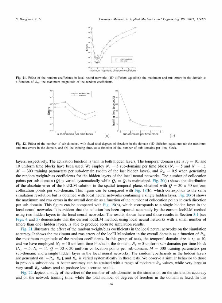
S. Dong and Z. Li Computer Methods in Applied Mechanics and Engineering 387 (2021) 114129
a
a
l
tpocstpluF(
ata(saiv
a
Fig. 21. Effect of the random coefficients in local neural networks (1D diffusion equation): the maximum and rms errors in the domain asfunction of Rm , the maximum magnitude of the random coefficients.
Fig. 22. Effect of the number of sub-domains, with fixed total degrees of freedom in the domain (1D diffusion equation): (a) the maximumnd rms errors in the domain, and (b) the training time, as a function of the number of sub-domains per time block.
ayers, respectively. The activation function is tanh in both hidden layers. The temporal domain size is t f = 10, and10 uniform time blocks have been used. We employ Ne = 5 sub-domains per time block (Nx = 5 and Nt = 1),M = 300 training parameters per sub-domain (width of the last hidden layer), and Rm = 0.5 when generatinghe random weight/bias coefficients for the hidden layers of the local neural networks. The number of collocationoints per sub-domain (Q) is varied systematically while Qx = Qt is maintained. Fig. 20(a) shows the distributionf the absolute error of the locELM solution in the spatial–temporal plane, obtained with Q = 30 × 30 uniformollocation points per sub-domain. This figure can be compared with Fig. 18(b), which corresponds to the sameimulation resolution but is obtained with local neural networks containing a single hidden layer. Fig. 20(b) showshe maximum and rms errors in the overall domain as a function of the number of collocation points in each directioner sub-domain. This figure can be compared with Fig. 19(b), which corresponds to a single hidden layer in theocal neural networks. It is evident that the solution has been captured accurately by the current locELM methodsing two hidden layers in the local neural networks. The results shown here and those results in Section 3.1 (seeigs. 4 and 5) demonstrate that the current locELM method, using local neural networks with a small number ofmore than one) hidden layers, is able to produce accurate simulation results.
Fig. 21 illustrates the effect of the random weight/bias coefficients in the local neural networks on the simulationccuracy. It shows the maximum and rms errors of the locELM solution in the overall domain as a function of Rm ,he maximum magnitude of the random coefficients. In this group of tests, the temporal domain size is t f = 10,nd we have employed Nb = 10 uniform time blocks in the domain, Ne = 5 uniform sub-domains per time blockNx = 5, Nt = 1), Q = 30 × 30 uniform collocation points per sub-domain, M = 300 training parameters perub-domain, and a single hidden layer in the local neural networks. The random coefficients in the hidden layersre generated on [−Rm, Rm], and Rm is varied systematically in these tests. We observe a similar behavior to thosen previous subsections. A better accuracy can be attained with a range of moderate Rm values, while very large orery small Rm values tend to produce less accurate results.
Fig. 22 depicts a study of the effect of the number of sub-domains in the simulation on the simulation accuracynd on the network training time, while the total number of degrees of freedom in the domain is fixed. In this
34

S. Dong and Z. Li Computer Methods in Applied Mechanics and Engineering 387 (2021) 114129
t
t
a
p
cv
ctccoicotst
FAbauo1detLtclhm
slFaml
ano
group of tests, the temporal domain size is t f = 10, and we have used Nb = 10 time blocks in the overall spatial–emporal domain. The number of uniform sub-domains per time block is varied systematically between Ne = 1 andNe = 5 in the simulations, implemented by fixing Nt = 1 and varying Nx between 1 and 5. We set the number ofraining parameters per sub-domain (M), and the number of uniform collocation points per sub-domain (Q, withQx = Qt ), in a way such that the total number of training parameters per time block is fixed at Ne M = 1500nd the total number of collocation points per time block is approximately fixed at Ne Q ≈ 2500. Specifically,
M and Q in different cases are: M = 1500 and Q = 50 × 50 for 1 sub-domain per time block, M = 750 andQ = 35 × 35 for 2 uniform sub-domains per time block, M = 500 and Q = 29 × 29 for 3 uniform sub-domainser time block, M = 375 and Q = 25 × 25 for 4 uniform sub-domains per time block, and M = 300 and
Q = 22 × 22 for 5 uniform sub-domains per time block. We employ Rm = 3.0 when generating the randomoefficients for the case with one sub-domain per time block, which is approximately at the optimal range of Rm
alues for this case. We employ Rm = 1.0 when generating the random coefficients for the rest of the cases withNe = 2 ∼ 5 sub-domains per time block. Note that the case with one sub-domain per time block is equivalent to theonfiguration of a global ELM in the simulation. Fig. 22(a) shows a comparison of the maximum and rms errors inhe overall spatial–temporal domain as a function of the number of sub-domains per time block in the simulations. Itan be observed that the numerical errors with 2 or more sub-domains are comparable to or smaller than the errorsorresponding to one sub-domain in the simulations. Fig. 22(b) shows the neural-network training time as a functionf the number of sub-domains per time block. One can observe that the training time decreases significantly withncreasing number of sub-domains. Compared with the case of one sub-domain per time block, the training timeorresponding to 2 and more sub-domains in the simulations has been considerably reduced, e.g. 277 seconds withne sub-domain versus 79 seconds with 2 sub-domains. These results confirm and reinforce our observations withhe other problems that, compared with global ELM, the use of domain decomposition and locELM with multipleub-domains can significantly reduce the network training time, and hence the computational cost, while attaininghe same or sometimes even better accuracy in the simulation results.
Let us now compare the current locELM method with DGM and PINN for solving the 1D diffusion equation.ig. 23 compares distributions of the solutions and their absolute errors obtained using DGM and PINN with thedam and L-BFGS optimizers and using locELM. The temporal domain size is set to t f = 1 in these tests. Withoth DGM and PINN, the neural network consists of 4 hidden layers, with a width of 40 nodes and the tanhctivation function in each layer. With DGM, when computing the loss function we have divided the domain into 5niform sub-regions along the x direction, and computed the residual norm integral by the Gaussian quadrature rulen 20 × 20 Gauss–Lobatto–Legendre quadrature points in each sub-region. With PINN, we have employed a set of00 × 20 uniform collocation points (100 uniform points in x and 20 uniform points in t) in the spatial–temporalomain as the input to the network. For both DGM and PINN, the neural network has been trained for 135,000pochs with the Adam optimizer, with the learning rate coefficient decreasing gradually from 0.001 at the beginningo 2.5×10⁻⁶ at the end of the training. With the L-BFGS optimizer, the neural network has been trained for 36,000-BFGS iterations for both DGM and PINN. In the simulation with locELM, we employ Nb = 1 time block in
he spatial–temporal domain, Ne = 5 sub-domains (with Nx = 5, Nt = 1) per time block, Q = 30 × 30 uniformollocation points per sub-domain, M = 300 training parameters per sub-domain, 1 hidden layer in each of theocal neural networks, and Rm = 1.0 when generating the random hidden-layer coefficients. Both DGM and PINNave captured the solution reasonably well. But their error levels are considerably higher, by about five orders ofagnitude, than that of the locELM method (10−3 versus 10−8).A comparison of the solution and the error profiles of locELM, DGM and PINN is provided in Fig. 24. Fig. 24(a)
hows the solution profiles at t = 1.0 obtained using DGM and PINN (Adam/L-BFGS optimizers) and using theocELM method, together with that of the exact solution. The settings and the parameters correspond to those ofig. 23. The computed profiles all agree with the exact solution quite well. Fig. 24(b) compares profiles of thebsolute error at t = 1.0 obtained with DGM, PINN and the current method. The numerical error of the currentethod, which is at a level around 10−9, is significantly smaller than those from DGM and PINN, which are at a
evel around 10−4.In Table 4 we provide some further comparisons between locELM, DGM, and PINN in terms of the accuracy
nd the computational cost. Here we list the maximum and rms errors in the overall spatial–temporal domain, theumber of epochs or iterations in network training, and the training time of DGM/PINN with the Adam and L-BFGS
ptimizers and of the locELM method. The problem settings and the simulation parameters correspond to those of35

S. Dong and Z. Li Computer Methods in Applied Mechanics and Engineering 387 (2021) 114129
aa
ot
Fig. 23. Comparison between locELM, DGM and PINN (1D diffusion equation): Distributions of the solutions (left column) and theirbsolute errors (right column) computed using DGM with Adam (a,b) and L-BFGS (c,d), using PINN with Adam (e,f) and L-BFGS (g,h),nd using the current locELM method (i,j).
Fig. 24. Comparison between locELM, DGM and PINN (1D diffusion equation): Profiles of the solutions (a) and their absolute errors (b) att = 1.0 obtained using DGM and PINN (Adam/L-BFGS optimizers) and using locELM. The problem settings and the simulation parameterscorrespond to those of Fig. 23.
Fig. 23. The error levels and the computational cost of DGM and PINN are comparable. The data demonstrate aclear superiority of locELM to DGM and PINN, with the locELM errors five orders of magnitude smaller and thetraining time over two orders of magnitude less.
Let us next compare the current locELM method with the classical finite element method for solving the 1Ddiffusion equation. In Figs. 25(a) and (b) we compare profiles of the solutions and their absolute errors at t = 1.0,
btained using the current locELM method and the finite element method. The domain and problem settings in theseests correspond to those of Figs. 23(e,f), with a temporal domain size t f = 1. The simulation parameters for the
locELM computation also correspond to those of Figs. 23(e,f). For the FEM simulation, the diffusion equation (35a)
36

S. Dong and Z. Li Computer Methods in Applied Mechanics and Engineering 387 (2021) 114129
v
iisrtu
fiesnsbtobtctFt1
mv
Table 41D diffusion equation: comparison between DGM/PINN (Adam/L-BFGS optimizers) and locELM.The settings and parameters correspond to those of Fig. 23.
Method Maximum error rms error Epochs/iterations Training time(seconds)
DGM (Adam) 2.59e − 2 3.84e − 3 135,000 4194.5DGM (L-BFGS) 5.82e − 3 8.21e − 4 36,000 3201.4PINN (Adam) 1.81e − 2 2.62e − 3 135,000 3739.1PINN (L-BFGS) 7.51e − 3 9.27e − 4 36,000 3174.4locELM 5.82e − 8 6.25e − 9 0 28.4
Fig. 25. Comparison between locELM and FEM (1D diffusion equation): Profiles of (a) the solutions and (b) their absolute errors at t = 1.0,computed using the current locELM method and using the finite element method (FEM). (c) The FEM maximum and rms errors at t = 0.5ersus ∆t , showing the temporal second-order convergence rate of FEM.
s discretized in time by the second-order backward differentiation formula (BDF2), and the diffusion term is treatedmplicitly. We have employed a time step size ∆t = 0.00025 and 10,000 uniform linear elements to discretize thepatial domain. It is evident from these data that both the FEM and the current method have produced accurateesults. Fig. 25(c) shows the maximum and rms errors at t = 0.5 versus the time step size ∆t with FEM, showinghe second-order temporal convergence rate. In these tests a fixed mesh of 10,000 uniform linear elements has beensed, which accounts for the observed error saturation in Fig. 25(c) when ∆t becomes sufficiently small.
Table 5 provides a comparison of the accuracy and the computational cost of the locELM method and thenite element method. In these tests the temporal domain size is set to t f = 1. In the locELM simulations wemploy a single time block in the spatial–temporal domain, 5 uniform sub-domains in the time block, and severalets of collocation points/sub-domain and training parameters/sub-domain, a single hidden layer in the local neuraletworks, and Rm = 1.0 when generating the random coefficients. In the FEM simulations, we employ severalets of elements and ∆t values. The maximum error and the rms error in the overall spatial–temporal domain haveeen computed, and the wall time for the computation or network training have been recorded. In Table 5 we listhese errors and the wall time numbers corresponding to the different simulation cases with locELM and FEM. Webserve that the current method performs markedly better than FEM. The current method achieves a considerablyetter accuracy with the same computational cost as FEM, and it incurs a lower computational cost while achievinghe same accuracy as FEM. For example, the locELM case with (Q, M) = (20× 20, 250) has a computational costomparable to the FEM cases with 2000 elements and ∆t = 0.001 and with 5000 elements and ∆t = 0.002. Buthe numerical errors of locELM are considerably smaller, by around three orders of magnitude, than those of theEM cases. The locELM case with (Q, M) = (30× 30, 300) has a lower computational cost, by a factor of about
hree, and a considerably better accuracy, by a factor of nearly three orders of magnitude, than the FEM case with0,000 elements and ∆t = 0.0005.
All the above results are for the 1D diffusion equation. In Fig. 26 we show some results of the current locELMethod for the two-dimensional (2D) diffusion equation plus time. This test concerns the following initial/boundary
alue problem, on the spatial–temporal domain Ω = (x, y, t) | x ∈ [a1, b1], y ∈ [a2, b2], t ∈ [0, t f ],
∂u− ν
(∂2u
2 +∂2u
2
)= f (x, y, t), (37a)
∂t ∂x ∂y37
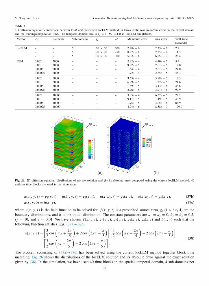
S. Dong and Z. Li Computer Methods in Applied Mechanics and Engineering 387 (2021) 114129
wbtf
Tmg
Table 51D diffusion equation: comparison between FEM and the current locELM method, in terms of the maximum/rms errors in the overall domainand the training/computation time. The temporal domain size is t f = 1. Rm = 1.0 in locELM simulations.
Method ∆t Elements Sub-domains Q M Maximum error rms error Wall time(seconds)
locELM – – 5 20 × 20 200 2.48e − 6 2.23e − 7 7.9– – 5 20 × 20 250 8.97e − 8 2.25e − 8 11.3– – 5 30 × 30 300 5.82e − 8 6.25e − 9 28.4
FEM 0.002 2000 – – – 2.42e − 4 4.40e − 5 5.90.001 2000 – – – 9.82e − 5 2.01e − 5 12.00.0005 2000 – – – 1.54e − 4 2.61e − 5 24.00.00025 2000 – – – 1.72e − 4 2.85e − 5 48.3
0.002 5000 – – – 3.63e − 4 5.98e − 5 12.30.001 5000 – – – 6.99e − 5 1.22e − 5 24.60.0005 5000 – – – 1.69e − 5 3.43e − 6 48.80.00025 5000 – – – 2.26e − 5 3.91e − 6 97.9
0.002 10000 – – – 3.85e − 4 6.32e − 5 22.20.001 10000 – – – 9.11e − 5 1.49e − 5 43.90.0005 10000 – – – 1.75e − 5 3.05e − 6 86.90.00025 10000 – – – 4.24e − 6 8.58e − 7 179.0
Fig. 26. 2D diffusion equation: distributions of (a) the solution and (b) its absolute error computed using the current locELM method. 40uniform time blocks are used in the simulation.
u(a1, y, t) = g1(y, t), u(b1, y, t) = g2(y, t), u(x, a2, t) = g3(x, t), u(x, b2, t) = g4(x, t), (37b)
u(x, y, 0) = h(x, y), (37c)
here u(x, y, t) is the field function to be solved for, f (x, y, t) is a prescribed source term, gi (1 ⩽ i ⩽ 4) are theoundary distributions, and h is the initial distribution. The constant parameters are a1 = a2 = 0, b1 = b2 = 0.5,f = 10, and ν = 0.01. We have chosen f (x, y, t), g1(y, t), g2(y, t), g3(x, t), g4(x, t) and h(x, y) such that theollowing function satisfies Eqs. (37a)–(37c),
u(x, y, t) =[
32
cos(
πx +2π
5
)+ 2 cos
(2πx −
π
5
)] [32
cos(
πy +2π
5
)+ 2 cos
(2πy −
π
5
)][
32
cos(
π t +2π
5
)+ 2 cos
(2π t −
π
5
)].
(38)
he problem consisting of (37a)–(37c) has been solved using the current locELM method together block timearching. Fig. 26 shows the distributions of the locELM solution and its absolute error against the exact solution
iven by (38). In the simulation, we have used 40 time blocks in the spatial–temporal domain, 4 sub-domains per
38

S. Dong and Z. Li Computer Methods in Applied Mechanics and Engineering 387 (2021) 114129
ufaTsdc
3
3
Ht
E
tC
sr
time block (with 2 uniform sub-domains along the x and y directions and one sub-domain in time), 15 × 15 × 15niform collocation points per sub-domain, a single hidden layer with a width of 400 nodes and the tanh activationunction in the local neural networks for each sub-domain, and the weight/bias coefficients for the hidden layerre set to uniform random values generated on the interval [−0.2, 0.2]. A seed value 12 has been used for theensorflow random number generator for this test. It can be observed that the current method has captured theolution accurately, with the maximum absolute error and the rms absolute error in the overall spatial–temporalomain being 1.04e − 6 and 7.19e − 8, respectively. The neural-network training time is 564 seconds for thisomputation.
.4. Nonlinear examples
.4.1. Nonlinear Helmholtz equationAs the first nonlinear example, we test the locELM method using the boundary value problem with the nonlinear
elmholtz equation in one dimension. Consider the domain [a, b] and the following boundary value problem onhis domain,
d2udx2 − λu + β sin(u) = f (x), (39a)
u(a) = h1, u(b) = h2, (39b)
where u(x) is the function to be solved for, f (x) is a prescribed source term, λ and β are constant parameters, andh1 and h2 are the boundary values. We assume the following values for the constant parameters involved in theseequations and domain specification,
a = 0, b = 8, λ = 50, β = 10.
We choose the source term f (x) and the boundary values h1 and h2 such that the following function satisfiesqs. (39a)–(39b),
u(x) = sin(
3πx +3π
20
)cos
(4πx −
2π
5
)+
32+
x10
. (40)
We employ the locELM method discussed in Section 2.3.1 for solving this problem, by restricting the methodo one dimension. We partition the domain [a, b] into Ne uniform sub-domains (sub-intervals), and impose the
1 continuity conditions across the sub-domain boundaries. We employ Q uniform collocation points within eachsub-interval.
The local neural network for each sub-domain consists of an input layer with one node (representing x), a singlehidden layer with M nodes and the tanh activation function, and an output layer with one node (representing thesolution u) and no activation function and no bias. An additional affine mapping operation normalizing the inputx data to the interval [−1, 1] is incorporated into the local neural networks right behind the input layer for eachub-domain. The weight and bias coefficients in the hidden layer of the local neural networks are set to uniformandom values generated on the interval [−Rm, Rm]. We employ a fixed seed value 12 for the Tensorflow random
number generator for all the tests reported in this sub-section with locELM.We employ the nonlinear least squared method with perturbations (NLSQ-perturb) and the combined New-
ton/linear least squared method (Newton-LLSQ) from Section 2.3.1 for computing the resultant nonlinear problem.The initial guess to the solution is set to zero in all the tests of this subsection. In the NLSQ-perturb method (seeAlgorithm 1), we have employed δ = 0.2, and ξ2 = 1 as discussed in Remark 2.8, for generating the randomperturbations in the following tests.
The locELM simulation parameters include the number of sub-domains (Ne), the number of collocation pointsper sub-domain (Q), the number of training parameters per sub-domain (M), and the maximum magnitude of therandom coefficients of the local neural networks (Rm).
Fig. 27 illustrates the profiles of the locELM solutions and their absolute errors computed using the NLSQ-perturband Newton-LLSQ methods. In these simulations, we have employed Ne = 4 uniform sub-domains, Q = 100uniform collocation points per sub-domain, M = 200 training parameters per sub-domain, and Rm = 5.0 for
generating the random weight/bias coefficients. The profile of the exact solution given by (40) is also included in39

S. Dong and Z. Li Computer Methods in Applied Mechanics and Engineering 387 (2021) 114129
ta
tTe
p
ct
Fig. 27. Nonlinear Helmholtz equation: profiles of the locELM solutions (a,c) and their absolute errors (b,d), computed using NLSQ-perturb(a,b) and Newton-LLSQ (c,d).
Fig. 28. Effect of collocation points (nonlinear Helmholtz equation): (a) the maximum and rms errors in the domain, and (b) the networkraining time, as a function of the number of collocation points per sub-domain, computed using the locELM method with NLSQ-perturbnd Newton-LLSQ.
hese plots. The solution profiles obtained with the current method exactly overlap with that of the exact solution.he error profiles indicate that the NLSQ-perturb method results in more accurate results than Newton-LLSQ, withrror levels on the order 10−12
∼ 10−9 for NLSQ-perturb versus 10−9∼ 10−5 for Newton-LLSQ.
Fig. 28 demonstrates the effect of the number of collocation points per sub-domain on the simulation accuracy andthe computational cost. In this group of tests, we have employed Ne = 4 sub-domains, M = 200 training parametersper sub-domain, and Rm = 5.0 when generating the random coefficients. The number of uniform collocation points
er sub-domain is varied systematically between Q = 25 and Q = 200. Fig. 28(a) shows the maximum and rmserrors in the domain as a function of the number of collocation points per sub-domain, obtained with NLSQ-perturband Newton-LLSQ. Fig. 28(b) shows the corresponding training time of the overall neural network versus thenumber of collocation points per sub-domain. With the Newton-LLSQ method, the errors are observed to decreasegradually with increasing number of collocation points, and appear to stagnate at a level around 10−6 when thenumber of collocation points/sub-domain is beyond 150. With the NLSQ-perturb method, the errors initially decreaseexponentially with increasing number of collocation points (when below 125), and then stagnate at a level around10−11 when the number of collocation points/sub-domain increases to 150 and beyond. The NLSQ-perturb resultsare in general considerably more accurate than those obtained with Newton-LLSQ. In terms of the training time, theNewton-LLSQ method is consistently faster than NLSQ-perturb, and the difference becomes larger as the number ofcollocation points increases. With the Newton-LLSQ method, the training time appears not sensitive to the numberof collocation points, and remains nearly the same with increasing number of collocation points (Fig. 28(b)). Withthe NLSQ-perturb method, the training time increases approximately linearly with increasing number of collocationpoints per sub-domain, and it becomes substantially slower than Newton-LLSQ when the number of collocationpoints becomes large.
Fig. 29 demonstrates the effect of the number of training parameters per sub-domain on the simulation accuracyand the computational cost. In this group of tests, we have employed Ne = 4 sub-domains, Q = 100 uniformollocation points per sub-domain, and Rm = 5.0 when generating the random coefficients in the hidden layers of
he local neural networks. The number of training parameters per sub-domain is varied systematically between 5040

S. Dong and Z. Li Computer Methods in Applied Mechanics and Engineering 387 (2021) 114129
ps
ape1dtdanpBmt
ide
Fig. 29. Effect of the number of training parameters (nonlinear Helmholtz equation): (a) the maximum and rms errors in the domain, and (b)the network training time, versus the number of training parameters per sub-domain, computed using the locELM method with NLSQ-perturband Newton-LLSQ.
Fig. 30. Results obtained with 2 hidden layers in local neural networks (nonlinear Helmholtz equation): profiles of (a) the locELM (NLSQ-erturb) solution and (b) its absolute error. (c) The maximum/rms errors in the domain versus the number of collocation points perub-domain.
nd 350. Fig. 29(a) shows the maximum and rms errors of the solutions as a function of the number of trainingarameters per sub-domain obtained with NLSQ-perturb and Newton-LLSQ. With NLSQ-perturb, the numericalrrors decrease substantially as the number of training parameters per sub-domain increases, reaching a level around0−10 when the number of training parameters increases beyond 200. With Newton-LLSQ, one can also observe aecrease in the errors as the number of training parameters increases. But the error reduction is much slower. Whenhe number of training parameters per sub-domain exceeds 200, the errors with Newton-LLSQ no longer seem toecrease further and remain at a level around 10−5. It is evident that the results from the Newton-LLSQ methodre generally much less accurate than those from the NLSQ-perturb method. Fig. 29(b) shows the correspondingetwork training time as a function of the number of training parameters per sub-domain. In the range of trainingarameters tested here, the training time with both of these two methods appear to fluctuate around a certain level.ut the training time with the Newton-LLSQ method is generally notably smaller than that with the NLSQ-perturbethod, except for the outlier point corresponding to 100 training parameters per sub-domain. These data suggest
hat Newton-LLSQ is generally faster than NLSQ-perturb.With the current locELM method, the local neural network can contain more than one hidden layer. As shown
n previous sub-sections, local neural networks with a small number (more than one) of hidden layers can alsoeliver accurate results using the current method. Fig. 30 demonstrates again this point with the nonlinear Helmholtzquation. In this group of tests, we employ Ne = 4 uniform sub-domains, M = 250 training parameters per sub-
domain, 2 hidden layers (with widths 25 and 250, respectively, and the tanh activation function) in each local neuralnetwork, and Rm = 2.0 when generating the random weight/bias coefficients for these hidden layers. The numberof uniform collocation points per sub-domain is varied systematically in these tests. Figs. 30(a) and (b) show thelocELM solution and error profiles obtained with Q = 175 uniform collocation points per sub-domain using the
NLSQ-perturb method. Fig. 30(c) shows the maximum and rms errors in the domain as a function of the number of41
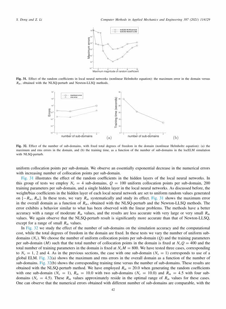
S. Dong and Z. Li Computer Methods in Applied Mechanics and Engineering 387 (2021) 114129
mw
uw
ttwoi
pttgsowdO
Fig. 31. Effect of the random coefficients in local neural networks (nonlinear Helmholtz equation): the maximum error in the domain versusRm , obtained with the NLSQ-perturb and Newton-LLSQ methods.
Fig. 32. Effect of the number of sub-domains, with fixed total degrees of freedom in the domain (nonlinear Helmholtz equation): (a) theaximum and rms errors in the domain, and (b) the training time, as a function of the number of sub-domains in the locELM simulationith NLSQ-perturb.
niform collocation points per sub-domain. We observe an essentially exponential decrease in the numerical errorsith increasing number of collocation points per sub-domain.Fig. 31 illustrates the effect of the random coefficients in the hidden layers of the local neural networks. In
his group of tests we employ Ne = 4 sub-domains, Q = 100 uniform collocation points per sub-domain, 200raining parameters per sub-domain, and a single hidden layer in the local neural networks. As discussed before, theeight/bias coefficients in the hidden layer of each local neural network are set to uniform random values generatedn [−Rm, Rm]. In these tests, we vary Rm systematically and study its effect. Fig. 31 shows the maximum errorn the overall domain as a function of Rm , obtained with the NLSQ-perturb and the Newton-LLSQ methods. The
error exhibits a behavior similar to what has been observed with the linear problems. The methods have a betteraccuracy with a range of moderate Rm values, and the results are less accurate with very large or very small Rm
values. We again observe that the NLSQ-perturb result is significantly more accurate than that of Newton-LLSQ,except for a range of small Rm values.
In Fig. 32 we study the effect of the number of sub-domains on the simulation accuracy and the computationalcost, while the total degrees of freedom in the domain are fixed. In these tests we vary the number of uniform sub-domains (Ne). We choose the number of uniform collocation points per sub-domain (Q) and the training parameters
er sub-domain (M) such that the total number of collocation points in the domain is fixed at Ne Q = 400 and theotal number of training parameters in the domain is fixed at Ne M = 800. We have tested three cases, correspondingo Ne = 1, 2 and 4. As in the previous sections, the case with one sub-domain (Ne = 1) corresponds to use of alobal ELM. Fig. 32(a) shows the maximum and rms errors in the overall domain as a function of the number ofub-domains. Fig. 32(b) shows the corresponding training time versus the number of sub-domains. These results arebtained with the NLSQ-perturb method. We have employed Rm = 20.0 when generating the random coefficientsith one sub-domain (Ne = 1), Rm = 10.0 with two sub-domains (Ne = 10.0) and Rm = 4.5 with four sub-omains (Ne = 4.5). These Rm values approximately reside in the optimal range of Rm values for these cases.
ne can observe that the numerical errors obtained with different number of sub-domains are comparable, with the42

S. Dong and Z. Li Computer Methods in Applied Mechanics and Engineering 387 (2021) 114129
t
egWa
Fig. 33. Nonlinear Helmholtz equation: Distributions of the solutions (a,c) and their absolute errors (b,d) computed using PINN [9] withhe Adam optimizer (a,b) and the L-BFGS optimizer (c,d). These can be compared with those in Fig. 27 computed using locELM.
Table 6Nonlinear Helmholtz equation: comparison between locELM and PINN in terms of the maxi-mum/rms errors in the domain, the number of epochs or nonlinear iterations, and the networktraining time. The problem settings and simulation parameters correspond to those of Figs. 27 and33.
Method Maximum error rms error Epochs/iterations Training time(seconds)
PINN (Adam) 4.56e − 3 5.04e − 4 45,000 578.2PINN (L-BFGS) 1.69e − 3 1.69e − 4 22,000 806.4locELM (NLSQ-perturb) 1.45e − 9 2.34e − 10 71 7.7locELM (Newton-LLSQ) 1.28e − 5 1.75e − 6 5 2.7
errors obtained on four sub-domains a little worse than those of the other cases. On the other hand, the networktraining time decreases significantly with increasing number of sub-domains.
We next compare the current locELM method with the PINN method [9] for solving the nonlinear Helmholtzquation. Fig. 33 shows distributions of the PINN solutions and their absolute errors against the exact solutioniven in Eq. (40), computed using the Adam optimizer (Figs. 33(a,b)) and the L-BFGS optimizer (Figs. 33(c,d)).ith the Adam optimizer, the neural network consists of 7 hidden layers, with a width of 50 nodes in each layer
nd the tanh activation function, in addition to the input layer of one node (representing x) and the output layer ofone node (representing the solution u). The network has been trained on the input data of 400 uniform collocationpoints for 45,000 epochs, with the learning rate gradually decreasing from 0.001 at the beginning to 5 × 10⁻⁶ atthe end of the training. With the L-BFGS optimizer, the neural network consists of 4 hidden layers, with a width of50 nodes in each layer and the tanh activation function, apart from the input layer of one node and the output layerof one node. The network has been trained on the input data of 400 uniform collocation points in the domain for22,000 L-BFGS iterations. The results indicate that the PINN method has captured the solution quite accurately,with the errors on the order 10−5
∼ 10−3 with the Adam optimizer and on the order 10−5∼ 10−4 with the L-BFGS
optimizer. Comparing the PINN results in this figure and the locELM results in Fig. 27, we can observe that thelocELM method is considerably more accurate than PINN.
Table 6 provides further comparisons between locELM and PINN in terms of the accuracy and the computationalcost. Here we have listed the maximum and rms errors in the domain, the number of epochs or nonlinear iterations inthe training, and the network training time, associated with the PINN (with Adam/L-BFGS optimizers) simulationsand the current locELM simulations. The problem settings and the simulation parameters here correspond to thosein Fig. 27 with locELM and those in Fig. 33 with PINN. It is evident that the current locELM method is muchmore accurate than PINN. For example, the errors obtained using locELM/NLSQ-perturb are about six orders ofmagnitude smaller than those obtained by PINN/L-BFGS. The errors obtained by locELM/Newton-LLSQ are abouttwo orders of magnitude smaller than those of PINN/L-BFGS. Furthermore, the current method is computationallymuch cheaper than PINN, with the training time approximately two orders of magnitude smaller (e.g. about 8seconds with locELM/NLSQ-perturb versus around 806 seconds with PINN/L-BFGS).
Let us now compare the current locELM method with the finite element method for solving the nonlinearHelmholtz equation. Fig. 34 shows the profiles of the finite element solution and its absolute error against the analyticsolution, computed on a mesh of 200,000 uniform elements. The finite element method is again implemented
using the FEniCS library in Python, and the nonlinear algebraic equation is solved using a Newton iteration. The43

S. Dong and Z. Li Computer Methods in Applied Mechanics and Engineering 387 (2021) 114129
mmal(l
Fig. 34. Nonlinear Helmholtz equation: profiles of the solution (a) and its absolute error (b) computed using the finite element method(FEM) with 200,000 uniform elements.
Table 7Nonlinear Helmholtz equation: comparison between locELM and FEM, in terms of the maximum/rms errors in the domain and thetraining/computation time. The problem settings correspond to those of Figs. 27(a,b) and 34.
Method Elements Sub-domains Q M Maximum error rms error Wall-time(seconds)
locELM (NLSQ-perturb) – 4 100 200 1.45e − 9 2.34e − 10 7.7– 4 125 200 3.96e − 11 7.02e − 12 10.6
FEM 200,000 – – – 5.26e − 9 1.37e − 9 4.7400,000 – – – 1.31e − 9 3.43e − 10 8.8800,000 – – – 3.29e − 10 8.57e − 11 18.1
FEM result is observed to be accurate, with an error level on the order 10−9. In Table 7 we compare the locELMethod and the finite element method with regard to the accuracy and the computational cost. The table lists theaximum and rms errors in the domain and the wall time of the training or computation, obtained using locELM
nd FEM on several sets of parameters corresponding to different simulation resolutions. One can observe thatocELM exhibits a comparable, and generally superior, performance to FEM. For example, the locELM case withQ, M) = (100, 200) has a computational cost comparable to the FEM case with 400,000 elements, and their errorevels are also comparable. The locELM case with (Q, M) = (125, 200) has a lower cost (∼ 10 seconds) than
the FEM case with 800,000 elements (∼ 18 seconds), and also has considerably smaller errors, by an order ofmagnitude, than the latter.
3.4.2. Nonlinear spring equationIn the next example we test the locELM method using an initial value problem, the nonlinear spring. The goal
here is to assess the performance of the locELM method together with the block time marching scheme, especiallyfor long-time dynamic simulations.
Consider the temporal domain, Ω = [0, t f ], and the following initial value problem on this domain,
d2udt2 + ω2u + α sin(u) = f (t), (41a)
u(0) = u0,dudt
t=0= v0, (41b)
where u(t) is the displacement, f (t) is an imposed external force, ω and α are constant parameters, u0 is the initialdisplacement, and v0 is the initial velocity. The parameters in the above domain and problem specifications assumethe following values in this subsection,
ω = 2, α = 0.5, t f = 100, or 15, or 2.5.
We choose the external force f (t) such that the following function satisfies Eq. (41a),
u(t) = t sin(t). (42)
44

S. Dong and Z. Li Computer Methods in Applied Mechanics and Engineering 387 (2021) 114129
t
vosdwlf(rbitg(
to
lct
ea
tteenbahmI
Fig. 35. Nonlinear spring: time histories of (a) the locELM solution and (b) its absolute error against the exact solution. 40 uniform timeblocks are used.
We set the initial displacement and the initial velocity both to zero, i.e. u0 = 0 and v0 = 0. Under these settings,he initial value problem consisting of Eqs. (41a)–(41b) has the solution given by (42).
We employ the locELM method and the block time marching scheme from Section 2.3.2 to solve this initialalue problem. We partition the domain [0, t f ] into Nb uniform time blocks, and solve this initial value problemn each time block individually and successively. For the computation within each time block, we use a singleub-domain in the simulation, as the amount of data involved in is quite small because the function does notepend on space. We enforce the equations on Q uniform collocation points within each time block. Accordingly,e employ a single neural network within each time block for this problem. The neural network consists of an input
ayer of one node (representing the time t), a single hidden layer with a width of M nodes and the tanh activationunction, and an output layer of one node (representing the solution u). The output layer is assumed to be linearno activation function) and contains no bias. As in previous sections, we incorporate an affine mapping operationight behind the input layer to normalize the input t data to the interval [−1, 1] for each time block. The weight andias coefficients in the hidden layer of the neural network are pre-set to uniform random values generated on thenterval [−Rm, Rm]. A fixed seed value 1234 is used with locELM for the random number generator. We employhe NLSQ-perturb method from Section 2.3.1 for computing the resultant nonlinear algebraic problem. The initialuess of the solution is set to zero. In the event the random perturbation is triggered, we employ δ = 1.0 and ξ2 = 1see Algorithm 1 and Remark 2.8) for generating the random perturbations in the tests of this subsection.
The locELM simulation parameters include the number of time blocks Nb, the number of collocation points perime block Q, the number of training parameters per time block M (i.e. the number of nodes in the hidden layerf the neural network), and the maximum magnitude of the random coefficients Rm .
Fig. 35 shows the time histories of the displacement and its absolute error obtained using locELM in a fairlyong-time simulation. The time history of the exact solution given by (42) has also been shown in Fig. 35(a) foromparison. In this test the domain size is set to t f = 100. We have employed Nb = 40 uniform time blocks withinhe domain, Q = 60 uniform collocation points per time block, M = 100 training parameters per time block, andRm = 5.0 when generating the random weight/bias coefficients for the hidden layer of the neural network. It isvident that the current locELM method has captured the solution very accurately, with the maximum level of thebsolute error on the order 10−8 over the entire domain.
Fig. 36 illustrates the effect of the number of degrees of freedom (collocation points, training parameters) onhe simulation accuracy. In this group of tests the temporal domain size is set to t f = 15, and we employ Nb = 6ime blocks within the domain. Fig. 36(a) shows the absolute-error histories of the locELM solution against thexact solution, obtained using 20 and 40 collocation points per time block. Fig. 36(b) shows the maximum and rmsrrors in the overall domain obtained with different numbers of collocation points in the locELM simulation. Theumber of training parameters per time block is fixed at M = 100 with the tests in these two plots. The errors cane observed to decrease exponentially as the number of collocation points per time block increases (when belowround 60), and then become stagnant as the number of collocation points increases further. Fig. 36(c) shows timeistories of the absolute errors corresponding to 20 and 40 training parameters per time block. Fig. 36(d) shows theaximum/rms errors in the overall domain, obtained with different numbers of training parameters per time block.
n the tests of these two plots, the number of collocation points per time block has been fixed at Q = 60. The
45

S. Dong and Z. Li Computer Methods in Applied Mechanics and Engineering 387 (2021) 114129
c
co(
aibita
sA
Fig. 36. Nonlinear spring: (a) Error histories obtained with 20 and 40 collocation points per time block. (b) The maximum/rms errors in thedomain versus the number of collocation points per time block. In (a) and (b), the number of training parameters per time block is fixedat 100. (c) Error histories obtained with 20 and 30 training parameters per time block. (d) The maximum/rms errors versus the number oftraining parameters per time block. In (c) and (d) the number of the collocation points per time block is fixed at 60.
Fig. 37. Nonlinear spring: The maximum and rms errors in the overall domain as a function of Rm , the maximum magnitude of the randomoefficients.
Fig. 38. Comparison between locELM and PINN (nonlinear spring): Time histories of (a) the solutions and (b) their absolute errors, computedusing PINN [9] with the Adam optimizer and using locELM with the NLSQ-perturb method. The temporal domain size is t f = 2.5.
onvergence with respect to the training parameters is not as regular as that for the collocation points. Nonetheless,ne can see that the errors approximately decrease exponentially with increasing number of training parameterswhen below 50), and then they essentially stagnate as the number of training parameters increases further.
Fig. 37 demonstrates the effect of Rm , the maximum magnitude of the random coefficients, on the simulationccuracy. In this set of tests, the temporal domain size is t f = 15. We have employed Nb = 6 uniform time blocksn the domain, Q = 60 uniform collocation points in each time block, and M = 100 training parameters per timelock. The value of Rm is varied systematically in the tests. In this figure we plot the maximum and rms errorsn the overall domain corresponding to different Rm values. The characteristics observed here are consistent withhose from previous subsections. The locELM method has a better accuracy with Rm in a range of moderate values,nd in this case approximately Rm = 1 ∼ 9. The results are less accurate if Rm is very large or very small.
Let us next compare the current locELM method with PINN [9] for solving the nonlinear spring equation. Fig. 38hows a comparison of the time histories of the solutions and their absolute errors obtained using PINN with thedam optimizer and using the current locELM method with NLSQ-perturb. In this group of tests, the temporal
46

S. Dong and Z. Li Computer Methods in Applied Mechanics and Engineering 387 (2021) 114129
(o
l
W
s
mesd
Table 8Nonlinear spring: Comparison between locELM and PINN in terms of the maximum/rms errors in thedomain, the number of epochs or nonlinear iterations in the training, and the network training time. Theproblem settings and the simulation parameters correspond to those of Fig. 38.
Method Maximum error rms error Epochs/iterations Training time(seconds)
PINN (Adam) 1.21e − 4 6.71e − 5 20,000 26.3locELM (NLSQ-perturb) 2.82e − 11 1.12e − 11 48 0.34
domain size is set to t f = 2.5. In the PINN simulation, the neural network consists of an input layer of one noderepresenting t), three hidden layers with a width of 10 nodes and the tanh activation function in each layer, and anutput layer of one node (representing the solution u). The input data consists of 500 uniform collocation points
from the domain [0, t f ]. The neural network has been trained using the Adam optimizer for 20,000 epochs, with theearning rate decreasing from 0.01 at the beginning to 1e− 5 at the end of the training. In the locELM simulation,
we employ a single time block (Nb = 1) in the domain, Q = 60 uniform collocation points within the time block,M = 100 training parameters in the time block, a single hidden layer in the neural network, and Rm = 5.0 forgenerating the random weight/bias coefficients. Fig. 38 demonstrates that both PINN and locELM have capturedthe solution accurately, but the error of the locELM result is considerably smaller than that of PINN.
Table 8 provides a further comparison between locELM and PINN in terms of their accuracy and computationalcost. The problem settings and the simulation parameters here correspond to those of Fig. 38. We have listed themaximum and rms errors of the PINN and locELM results in the overall domain, the number of epochs or nonlineariterations in the training, and the network training time. The data demonstrate that the current locELM method ismuch more accurate, by six orders of magnitude, than PINN, and the network training time of locELM is muchsmaller, by nearly two orders of magnitude, than that of PINN.
3.4.3. Viscous Burger’s equationIn this subsection we further test the locELM method using the viscous Burger’s equation. Consider the spatial–
temporal domain Ω = (x, t) | x ∈ [a, b], t ∈ [0, t f ], and the following initial/boundary value problem with theBurger’s equation,
∂u∂t+ u
∂u∂x= ν
∂2u∂x2 + f (x, t), (43a)
u(a, t) = g1(t), u(b, t) = g2(t), (43b)
u(x, 0) = h(x), (43c)
where u(x, t) is the solution to be solved for, the constant ν denotes the viscosity, f (x, t) is a prescribed sourceterm, g1(t) and g2(t) denote the boundary distributions, and h(x) is the initial distribution. We employ the followingvalues for the constant parameters,
ν = 0.01, a = 0, b = 5, t f = 10, or 2.5, or 0.25.
e choose the source term f and the boundary/initial distributions (g1, g2 and h) such that the function
u(x, t) =(
1+x10
)(1+
t10
)[2 cos
(πx +
2π
5
)+
32
cos(
2πx −3π
5
)][2 cos
(π t +
2π
5
)+
32
cos(
2π t −3π
5
)] (44)
atisfies this initial/boundary value problem.We employ the method from Section 2.3.2 with block time marching to solve this problem, by restricting the
ethod to one spatial dimension. The spatial–temporal domain Ω is partitioned into Nb uniform time blocks. Withinach time block, we further partition its spatial–temporal domain into Nx uniform sub-domains in x and Nt uniformub-domains in time, resulting in Ne = Nx Nt sub-domains per time block. C1 continuity is imposed on the sub-omain boundaries in the x direction, and C0 continuity is imposed on the sub-domain boundaries in time. Within
47
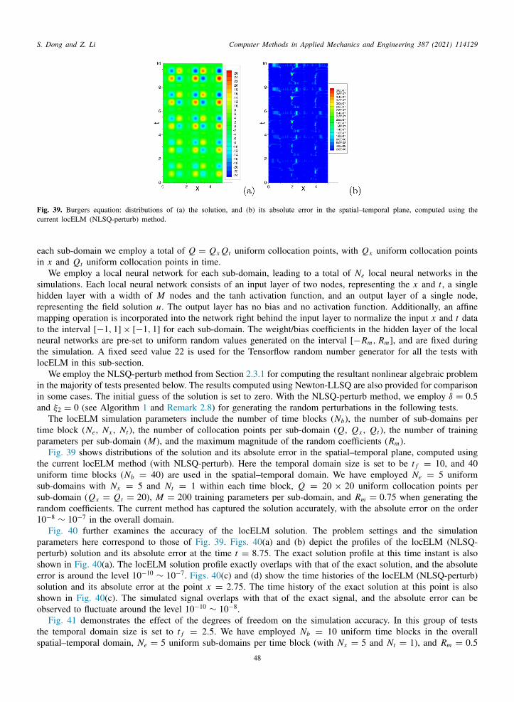
S. Dong and Z. Li Computer Methods in Applied Mechanics and Engineering 387 (2021) 114129
c
e
shrmtntl
iia
tp
tussr1
ppsesso
ts
Fig. 39. Burgers equation: distributions of (a) the solution, and (b) its absolute error in the spatial–temporal plane, computed using theurrent locELM (NLSQ-perturb) method.
ach sub-domain we employ a total of Q = Qx Qt uniform collocation points, with Qx uniform collocation pointsin x and Qt uniform collocation points in time.
We employ a local neural network for each sub-domain, leading to a total of Ne local neural networks in theimulations. Each local neural network consists of an input layer of two nodes, representing the x and t , a singleidden layer with a width of M nodes and the tanh activation function, and an output layer of a single node,epresenting the field solution u. The output layer has no bias and no activation function. Additionally, an affineapping operation is incorporated into the network right behind the input layer to normalize the input x and t data
o the interval [−1, 1]× [−1, 1] for each sub-domain. The weight/bias coefficients in the hidden layer of the localeural networks are pre-set to uniform random values generated on the interval [−Rm, Rm], and are fixed duringhe simulation. A fixed seed value 22 is used for the Tensorflow random number generator for all the tests withocELM in this sub-section.
We employ the NLSQ-perturb method from Section 2.3.1 for computing the resultant nonlinear algebraic problemn the majority of tests presented below. The results computed using Newton-LLSQ are also provided for comparisonn some cases. The initial guess of the solution is set to zero. With the NLSQ-perturb method, we employ δ = 0.5nd ξ2 = 0 (see Algorithm 1 and Remark 2.8) for generating the random perturbations in the following tests.
The locELM simulation parameters include the number of time blocks (Nb), the number of sub-domains perime block (Ne, Nx , Nt ), the number of collocation points per sub-domain (Q, Qx , Qt ), the number of trainingarameters per sub-domain (M), and the maximum magnitude of the random coefficients (Rm).
Fig. 39 shows distributions of the solution and its absolute error in the spatial–temporal plane, computed usinghe current locELM method (with NLSQ-perturb). Here the temporal domain size is set to be t f = 10, and 40niform time blocks (Nb = 40) are used in the spatial–temporal domain. We have employed Ne = 5 uniformub-domains with Nx = 5 and Nt = 1 within each time block, Q = 20 × 20 uniform collocation points perub-domain (Qx = Qt = 20), M = 200 training parameters per sub-domain, and Rm = 0.75 when generating theandom coefficients. The current method has captured the solution accurately, with the absolute error on the order0−8∼ 10−7 in the overall domain.
Fig. 40 further examines the accuracy of the locELM solution. The problem settings and the simulationarameters here correspond to those of Fig. 39. Figs. 40(a) and (b) depict the profiles of the locELM (NLSQ-erturb) solution and its absolute error at the time t = 8.75. The exact solution profile at this time instant is alsohown in Fig. 40(a). The locELM solution profile exactly overlaps with that of the exact solution, and the absoluterror is around the level 10−10
∼ 10−7. Figs. 40(c) and (d) show the time histories of the locELM (NLSQ-perturb)olution and its absolute error at the point x = 2.75. The time history of the exact solution at this point is alsohown in Fig. 40(c). The simulated signal overlaps with that of the exact signal, and the absolute error can bebserved to fluctuate around the level 10−10
∼ 10−8.Fig. 41 demonstrates the effect of the degrees of freedom on the simulation accuracy. In this group of tests
he temporal domain size is set to t f = 2.5. We have employed Nb = 10 uniform time blocks in the overallpatial–temporal domain, N = 5 uniform sub-domains per time block (with N = 5 and N = 1), and R = 0.5
e x t m48

S. Dong and Z. Li Computer Methods in Applied Mechanics and Engineering 387 (2021) 114129
lt
pos
dadnbacts
wdh
Fig. 40. Burger’s equation: Profiles of the locELM (NLSQ-perturb) solution (a) and its absolute error (b) at t = 8.75. Time histories of theocELM (NLSQ-perturb) solution (c) and its absolute error (d) at the point x = 2.75. The settings and simulation parameters correspond tohose of Fig. 39.
Fig. 41. Effect of the degrees of freedom on the accuracy (Burger’s equation): the maximum and rms errors in the domain as a functionof (a) the number of collocation points in each direction per sub-domain, and (b) the number of training parameters per sub-domain.
when generating random coefficients for the hidden layers of the local neural networks. First, we fix the numberof training parameters per sub-domain to M = 200, and vary the number of (uniform) collocation points per sub-domain systematically while maintaining Qx = Qt . Fig. 41(a) shows the maximum and rms errors in the overalldomain versus the number of collocation points in each direction per sub-domain. It is observed that the errorsdecrease essentially exponentially with increasing number of collocation points per direction (when below aroundQx = Qt = 15). Then the errors stagnate as the number of collocation points per direction increases beyond15, due to the saturation associated with the fixed number of training parameters in the test. Then, we fix thenumber of uniform collocation points to Q = 20× 20 per sub-domain, and vary the number of training parameters
er sub-domain systematically in a range of values. Fig. 41(b) shows the resultant maximum/rms errors in theverall domain versus the number of training parameters per sub-domain. As the number of training parameters perub-domain increases, the locELM errors can be observed to decrease substantially.
Fig. 42 demonstrates the effect of the number of sub-domains, with the total number of degrees of freedom in theomain (approximately) fixed. In this group of tests, the temporal domain size is set to t f = 0.25, and we employsingle time block in the spatial–temporal domain. We employ uniform sub-domains, and vary the number of sub-omains within the time block systematically between Ne = 1 and Ne = 5 (with fixed Nt = 1 and various Nx ). Theumber of (uniform) collocation points per sub-domain and the number of training parameters per sub-domain areoth varied, but the total number of collocation points and the total number of training parameters in the time blockre fixed approximately at Ne Q ≈ 2000 and Ne M ≈ 1000, respectively. More specifically, we employ Q = 45×45ollocation points/sub-domain and M = 1000 training parameters/sub-domain with Ne = 1 sub-domain within theime block, Q = 32×32 collocation points/sub-domain and M = 500 training parameters/sub-domain with Ne = 2ub-domains, Q = 26 × 26 collocation points/sub-domain and M = 333 training parameters/sub-domain with
Ne = 3 sub-domains, Q = 22 × 22 collocation points/sub-domain and M = 250 training parameters/sub-domainith Ne = 4 sub-domains, and Q = 20× 20 collocation points/sub-domain and M = 200 training parameters/sub-omain with Ne = 5 sub-domains within the time block. When generating the random weight/bias coefficients, weave employed Rm = 2.0 with Ne = 1 sub-domain in the time block, Rm = 1.0 with Ne = 2 and 3 sub-domains, and
Rm = 0.75 with Ne = 4 and 5 sub-domains within the time block. These values are approximately in the optimal
49

S. Dong and Z. Li Computer Methods in Applied Mechanics and Engineering 387 (2021) 114129
((
r
Fig. 42. Effect of the number of sub-domains, with fixed total degrees of freedom in the domain (Burger’s equation): (a) the maximum andrms errors in the domain, and (b) the training time, as a function of the number of uniform sub-domains per time block. Temporal domainsize is t f = 0.25, and a single time block is used in the spatial–temporal domain.
Fig. 43. Comparison between locELM and DGM (Burger’s equation): distributions of the solutions (left column) and their absolute errorsright column) computed using DGM with the Adam optimizer (a,b) and L-BFGS optimizer (c,d), and using locELM with NLSQ-perturbe,f) and with Newton-LLSQ (g,h).
ange of Rm values for these cases. Fig. 42(a) shows the maximum and rms errors of the locELM (NLSQ-perturb)solution in the domain as a function of the number of sub-domains within the time block. We observe that theerrors decrease quite significantly, by nearly two orders of magnitude, as the number of sub-domains increasesfrom Ne = 1 to Ne = 3. The errors remain approximately at the same level with three and more sub-domains.Note that the case with one sub-domain corresponds to the global ELM computation. These results indicate thatthe local ELM simulation with multiple sub-domains appears to achieve a better accuracy than the global ELMsimulation for this problem. Fig. 42(b) shows the training time of the neural network as a function of the number ofsub-domains. The training time has been reduced substantially as the number of sub-domains increases from one tothree sub-domains (from around 110 seconds to about 40 seconds), and it remains approximately the same with threeand more sub-domains. These results show that, compared with the global ELM, the use of domain decompositionand multiple sub-domains in locELM can significantly reduce the computational cost for the Burger’s equation.This is consistent with the observations with the other problems in previous sections.
We next compare the current locELM method with the deep Galerkin method (DGM) for the Burger’s equation.Fig. 43 is a comparison of distributions of the solutions (left column) and their absolute errors (right column)in the spatial–temporal plane, obtained using DGM with the Adam and L-BFGS optimizers (top two rows) and
using the current locELM method with NLSQ-perturb and Newton-LLSQ (bottom two rows). In these tests the50
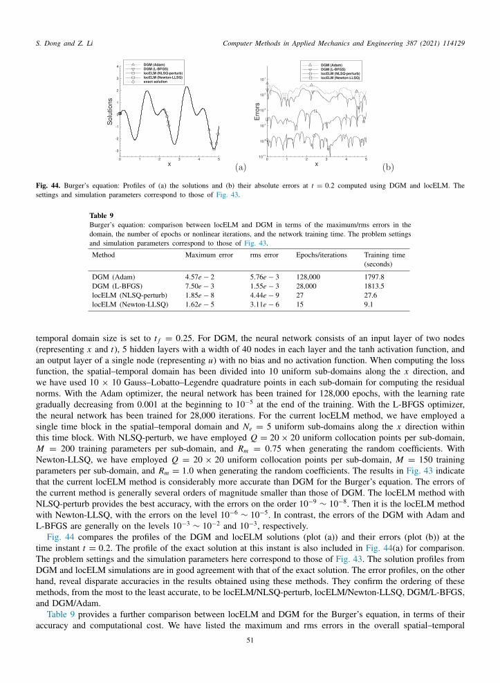
S. Dong and Z. Li Computer Methods in Applied Mechanics and Engineering 387 (2021) 114129
s
Fig. 44. Burger’s equation: Profiles of (a) the solutions and (b) their absolute errors at t = 0.2 computed using DGM and locELM. Theettings and simulation parameters correspond to those of Fig. 43.Table 9Burger’s equation: comparison between locELM and DGM in terms of the maximum/rms errors in thedomain, the number of epochs or nonlinear iterations, and the network training time. The problem settingsand simulation parameters correspond to those of Fig. 43.
Method Maximum error rms error Epochs/iterations Training time(seconds)
DGM (Adam) 4.57e − 2 5.76e − 3 128,000 1797.8DGM (L-BFGS) 7.50e − 3 1.55e − 3 28,000 1813.5locELM (NLSQ-perturb) 1.85e − 8 4.44e − 9 27 27.6locELM (Newton-LLSQ) 1.62e − 5 3.11e − 6 15 9.1
temporal domain size is set to t f = 0.25. For DGM, the neural network consists of an input layer of two nodes(representing x and t), 5 hidden layers with a width of 40 nodes in each layer and the tanh activation function, andan output layer of a single node (representing u) with no bias and no activation function. When computing the lossfunction, the spatial–temporal domain has been divided into 10 uniform sub-domains along the x direction, andwe have used 10 × 10 Gauss–Lobatto–Legendre quadrature points in each sub-domain for computing the residualnorms. With the Adam optimizer, the neural network has been trained for 128,000 epochs, with the learning rategradually decreasing from 0.001 at the beginning to 10−5 at the end of the training. With the L-BFGS optimizer,the neural network has been trained for 28,000 iterations. For the current locELM method, we have employed asingle time block in the spatial–temporal domain and Ne = 5 uniform sub-domains along the x direction withinthis time block. With NLSQ-perturb, we have employed Q = 20× 20 uniform collocation points per sub-domain,M = 200 training parameters per sub-domain, and Rm = 0.75 when generating the random coefficients. WithNewton-LLSQ, we have employed Q = 20 × 20 uniform collocation points per sub-domain, M = 150 trainingparameters per sub-domain, and Rm = 1.0 when generating the random coefficients. The results in Fig. 43 indicatethat the current locELM method is considerably more accurate than DGM for the Burger’s equation. The errors ofthe current method is generally several orders of magnitude smaller than those of DGM. The locELM method withNLSQ-perturb provides the best accuracy, with the errors on the order 10−9
∼ 10−8. Then it is the locELM methodwith Newton-LLSQ, with the errors on the level 10−6
∼ 10−5. In contrast, the errors of the DGM with Adam andL-BFGS are generally on the levels 10−3
∼ 10−2 and 10−3, respectively.Fig. 44 compares the profiles of the DGM and locELM solutions (plot (a)) and their errors (plot (b)) at the
time instant t = 0.2. The profile of the exact solution at this instant is also included in Fig. 44(a) for comparison.The problem settings and the simulation parameters here correspond to those of Fig. 43. The solution profiles fromDGM and locELM simulations are in good agreement with that of the exact solution. The error profiles, on the otherhand, reveal disparate accuracies in the results obtained using these methods. They confirm the ordering of thesemethods, from the most to the least accurate, to be locELM/NLSQ-perturb, locELM/Newton-LLSQ, DGM/L-BFGS,and DGM/Adam.
Table 9 provides a further comparison between locELM and DGM for the Burger’s equation, in terms of their
accuracy and computational cost. We have listed the maximum and rms errors in the overall spatial–temporal51

S. Dong and Z. Li Computer Methods in Applied Mechanics and Engineering 387 (2021) 114129
cF
TBt
Bl
eWsicatodsFt
f
Fig. 45. Comparison between locELM and FEM (Burger’s equation): Profiles of (a) the solutions and (b) their absolute errors at t = 0.2,omputed using locELM (with NLSQ-perturb) and using FEM. (c) The maximum and rms errors at t = 0.25 versus ∆t computed usingEM (with a mesh of 10,000 uniform elements), showing its second-order convergence rate in time.
able 10urger’s equation: comparison between locELM and FEM in terms of the maximum/rms errors in the domain and the training/computation
ime. Q and M denote the number of collocation points per sub-domain and the number of training parameters per sub-domain, respectively.
Method Elements ∆t Sub-domains Q M Maximum error rms error Wall-time(seconds)
locELM – – 5 15 × 15 150 2.10e − 6 4.35e − 7 14.7(NLSQ-perturb) – – 5 20 × 20 200 1.85e − 8 4.44e − 9 27.6
locELM – – 5 15 × 15 150 1.25e − 5 2.71e − 6 6.8(Newton-LLSQ) – – 5 20 × 20 150 1.62e − 5 3.11e − 6 9.1
FEM 2000 0.00025 – – – 2.64e − 5 5.15e − 6 12.52000 0.000125 – – – 3.07e − 5 5.76e − 6 25.4
5000 0.00025 – – – 1.89e − 5 1.74e − 6 26.05000 0.000125 – – – 4.13e − 6 7.90e − 7 50.8
10000 0.00025 – – – 2.22e − 5 1.99e − 6 47.710000 0.000125 – – – 4.74e − 6 4.36e − 7 92.6
domain, the number of epochs or nonlinear iterations in the training, and the training time of the neural networkcorresponding to DGM with the Adam/L-BFGS optimizers and the current locELM method with NLSQ-perturband Newton-LLSQ. The observations here are consistent with those of previous sections. The locELM method isorders of magnitude more accurate than DGM (e.g. 10−8 with locELM/NLSQ-perturb versus 10−3 with DGM/L-
FGS), and its training time is orders of magnitude smaller than that of DGM (e.g. around 28 seconds withocELM/NLSQ-perturb versus around 1800 seconds with DGM/L-BFGS).
Finally, we compare the current locELM method with the classical finite element method for solving the Burger’squation. In the FEM simulation, we discretize the Burger’s equation (43a) in time using a semi-implicit scheme.e treat the nonlinear term explicitly and the viscous term implicitly, and discretize the time derivative by the
econd-order backward differentiation formula (BDF2). The method is again implemented using the FEniCS libraryn Python. Figs. 45(a) and (b) show a comparison of the solution and error profiles at t = 0.2 obtained using theurrent locELM (NLSQ-perturb) method and using the finite element method. Fig. 45(c) shows the numerical errorst t = 0.25 as a function of the time step size ∆t computed using the finite element method. In these simulationshe temporal domain size is t f = 0.25. In Figs. 45(a,b), the FEM simulation is conducted with ∆t = 1.25e − 4n a mesh of 10,000 uniform elements, and the locELM simulation is conducted with a single time block in theomain and Ne = 5 sub-domains in the time block, with (Q, M) = (20×20, 200) and Rm = 0.75. In Fig. 45(c), theimulations are performed with a fixed mesh of 10,000 uniform elements. It can be observed that both locELM andEM have produced accurate solutions, and that the FEM exhibits a second-order convergence rate in time before
he error saturation when ∆t becomes very small.Table 10 provides a comparison between locELM and FEM in terms of their accuracy and computational cost
or the Burger’s equation. The temporal domain size is t f = 0.25 in these tests. We solve the problem using
52

S. Dong and Z. Li Computer Methods in Applied Mechanics and Engineering 387 (2021) 114129
f
postp
wttdmot
P
locELM and FEM on several sets of simulation parameters with different numerical resolutions. The maximumand rms errors in the spatial–temporal domain are computed, and we also record the training time of locELM andthe computation time of FEM in these simulations. We list in this table the maximum and rms errors, as wellas the training/computation time, corresponding to different simulation parameters for the locELM method withNLSQ-perturb and Newton-LLSQ and for the finite element method. A single time block has been used in thespatial–temporal domain for the locELM simulations, and we employ Rm = 0.75 with locELM/NLSQ-perturb andRm = 1.0 with locELM/Newton-LLSQ for generating the random coefficients. It is observed that the current locELMmethod with both NLSQ-perturb and Newton-LLSQ shows a superior performance to the FEM. For example, thetwo cases with locELM/Newton-LLSQ have numerical errors comparable to the FEM cases with 2000 elements(for both ∆t), 5000 elements (∆t = 0.00025) and 10000 elements (∆t = 0.00025), but the computational cost oflocELM/Newton-LLSQ is notably smaller than the cost of these FEM cases. The locELM/NLSQ-perturb case with(Q, M) = (15× 15, 150) has numerical errors comparable to the FEM cases with 5000 elements (∆t = 0.000125)and 10000 elements (∆t = 0.000125), but the computational cost of this locELM/NLSQ-perturb case is only araction of those of these two FEM cases. The locELM/NLSQ-perturb case with (Q, M) = (20 × 20, 200) has
a computational cost comparable to the FEM cases with 2000 elements (∆t = 0.000125) and 5000 elements(∆t = 0.00025), but the errors of this locELM/NLSQ-perturb case are nearly three orders of magnitude smallerthan those of these two FEM cases.
4. Concluding remarks
In this paper we have developed an efficient method based on domain decomposition and local extreme learningmachines (termed locELM) for solving linear/nonlinear partial differential equations. The problem domain ispartitioned into sub-domains, and the field solution on each sub-domain is represented by a local shallow feed-forward neural network, consisting of a small number (one or more) of hidden layers. Ck continuity conditions,with k related to the PDE order, are imposed on the sub-domain boundaries. The hidden-layer coefficients of allthe local neural networks are pre-set to random values, and are fixed in the computation. The training parametersconsist of the output-layer coefficients of the local neural networks.
We employ a set of collocation points within each sub-domain, which constitute the input data to the neuralnetwork. The PDE, the boundary/initial conditions, and the Ck continuity conditions are enforced on the collocation
oints in the sub-domains, on the overall domain boundaries, and on the sub-domain boundaries, respectively. Theseperations result in a system of linear or nonlinear algebraic equations about the training parameters. We seek a leastquares solution to this system, and compute the solution by a linear or nonlinear least squares method. Traininghe overall network consists of the linear or nonlinear least squares computations. This is different from the backropagation-type algorithms.
For longer-time simulations of time-dependent PDEs, we have developed a block time-marching scheme togetherith the locELM method. The spatial–temporal domain is first divided into a number of windows in time, referred
o as time blocks, and we solve the PDE on each time block separately and successively. We observe that when theemporal dimension of the domain is large, if without block time marching, the neural network can become veryifficult to train. On the other hand, with block time marching and using a moderate time block size, the problem isore manageable and much easier to solve. Block time marching requires re-training of the overall neural network
n different time blocks, and so all network trainings are online operations. This is feasible with locELM thankso its high accuracy and low computational cost.
We have performed extensive numerical experiments to test the locELM method, and compared it with DGM,INN, global ELM, and the finite element method (FEM). We have the following observations:
• The locELM method exhibits a clear sense of convergence with increasing number of degrees of freedom. Itserrors typically decrease exponentially or nearly exponentially as the number of sub-domains, or the numberof collocation points/sub-domain, or the number of training parameters/sub-domain increases.• The random hidden-layer coefficients of the local neural networks influence the simulation accuracy. In this
work these coefficients are set to uniform random values generated on [−Rm, Rm]. The simulation accuracytends to decrease with very large or very small Rm . Higher accuracy is generally associated with a rangeof moderate Rm values. This range of optimal Rm values tends to expand when the number of collocationpoints/sub-domain or training parameters/sub-domain increases.
53

S. Dong and Z. Li Computer Methods in Applied Mechanics and Engineering 387 (2021) 114129
• The locELM training time generally increases linearly (or super-linearly for some problems) with respect tothe number of sub-domains. It also tends to increase with respect to the number of collocation points and tothe number of training parameters, but the relation is not quite regular.• When the total degrees of freedom (total collocation points, total training parameters) in the system are fixed,
increasing the number of sub-domains, hence with the number of collocation points/training parameters persub-domain accordingly reduced, generally leads to simulation results with comparable accuracy, but it candramatically reduce the network training time. Compared with global ELM, which corresponds to the locELMwith a single sub-domain, the use of multiple sub-domains in locELM can significantly reduce the networktraining time, and produce results with comparable accuracy.• The current locELM method shows a clear superiority to DGM and PINN, which are some of the commonly-
used DNN-based PDE solvers, in terms of both accuracy and computational cost. The numerical errors andthe network training time of locELM are considerably smaller, typically by orders of magnitude, than thoseof DGM and PINN.• The locELM method exhibits a computational performance that is comparable, and oftentimes superior, to the
classical FEM. With the same computational cost, the locELM errors are comparable to, and oftentimes muchsmaller than, the FEM errors. To achieve the same accuracy, the locELM training time is comparable to, andoftentimes markedly smaller than, the FEM computation time.
We would like to make some further comments with regard to Rm , the maximum magnitude of the randomhidden-layer coefficients of the local neural networks. As discussed above, the simulation results have a betteraccuracy if Rm falls into a range of moderate values for a given problem. Let us consider the following question:given a new problem (e.g. a new PDE), how do we know what this range is and how do we find this range ofoptimal Rm values in practice? The approximate range of these optimal Rm values can be estimated readily bypreliminary numerical experiments. Here is the basic idea. Given a new problem, one can always add some sourceterms to the PDE or to the boundary/initial conditions, and then manufacture a solution to the given problem,with the augmented source terms. Then one can use the manufactured solution to evaluate the accuracy of a setof preliminary simulations by varying the Rm systematically. This will provide a reasonable estimate for the rangeof optimal Rm values. After that, one can conduct actual simulations of the given problem, without the addedsource term, by using an Rm value from the estimated range. It is observed that the optimal range for Rm is notsensitive to the manufactured solution used for its estimate when a reasonably good resolution is employed. If avery complicated manufactured solution is being used, one will want to employ a large enough resolution whenestimating Rm .
Some further comments are also in order concerning the numerical tests with fixed total degrees of freedom inthe domain, while the number of sub-domains is varied. Because the total degrees of freedom in the domain is fixed,the degrees of freedom per sub-domain decrease as the number of sub-domains increases. One can anticipate that,when the number of sub-domains becomes sufficiently large, the number of degrees of freedom per sub-domaincan become very small. This will be bound to adversely affect the simulation accuracy, because the solution isrepresented locally by these degrees of freedom on each sub-domain. Therefore, if the total degrees of freedom inthe domain are fixed, when the number of sub-domains increases beyond a certain point, the simulation accuracywill start to deteriorate. The aforementioned observation about comparable accuracy with increasing number ofsub-domains, with fixed total degrees of freedom in the domain, is for the cases where the number of sub-domainsis below that point.
As demonstrated by ample examples in this paper, the computational performance of the current locELM methodis on par with, and oftentimes exceeds, that of the classical finite element method. The importance of this pointcannot be overstated. To the best of the authors’ knowledge, this seems to be the first time when a neural network-based method delivers the same performance as, or a better performance than, a traditional numerical method forthe commonly-encountered computational problems in low dimensions. The current method demonstrates the greatpotential, and perhaps points toward a path forward, for neural network-based methods to be truly competitive, andexcel, in computational science and engineering simulations.
Some characteristics exhibited by the current locELM method, e.g. the exponential convergence with respectto the number of collocation points and training parameters, are reminiscent of those of the traditional high-ordernumerical methods. Compared with the finite element method employing higher-order elements (see Appendix B),
the current locELM method is also competitive to a certain degree. But overall the locELM seems not as efficient54

S. Dong and Z. Li Computer Methods in Applied Mechanics and Engineering 387 (2021) 114129
h
A
A
cl
fi
as the higher-order finite elements at this point. How to further improve this method is an interesting problem, andwill be explored in a future endeavor.
Declaration of competing interest
The authors declare that they have no known competing financial interests or personal relationships that couldave appeared to influence the work reported in this paper.
cknowledgment
This work was partially supported by NSF, USA (DMS-2012415, DMS-1522537).
ppendix A. The Newton-Linear Least Squares (Newton-LLSQ) method
In this Appendix we elaborate on the Newton-LLSQ method from Section 2.3.1 for solving the nonlinear systemonsisting of (22a)–(22b) in some detail. This method combines the Newton iteration on the top level with a lineareast squares approach for computing the increment field within each Newton step.
Let u(k)(x, y) denote the approximation of the solution u at the Newton step k, and v(x, y) denote the incrementeld to be computed at this step. Then
u(k+1)= u(k)
+ v. (45)
The increment v is described by the linearized version of Eq. (22a),
Lv + J(u(k), u(k)
x , u(k)y
)v = f (x, y)−
[Lu(k)
+ F(u(k), u(k)
x , u(k)y
)], (46)
where u(k)x and u(k)
y denote the partial derivatives of u(k), and J(u(k), u(k)
x , u(k)y
)is the Jacobian (operator) of the
nonlinear term F(u, ux , u y). We impose the boundary condition (22b) on u(k+1), which gives rise to followingboundary condition for the increment v in light of (45),
v = g(x, y)− u(k)(x, y), on ∂Ω . (47)
Eqs. (46) and (47) are linear equations about the increment field v(x, y). Given the approximation u(k) at Newtonstep k, these equations can be solved using the locELM method for linear differential equations as discussed inSection 2.2.1, which employs a linear least squares approach. Then the approximation to the solution u at Newtonstep (k + 1) is given by Eq. (45).
Note that in Section 2.3.1 we assume that L is a second-order linear differential operator with respect to both xand y. When solving the Eqs. (46)–(47) with locELM, we therefore impose the C1 continuity conditions for u(k+1)
on the sub-domain boundaries. These will give rise to the continuity conditions about the increment field v onthe sub-domain boundaries. Let the vectors [X0, X1, . . . , X Nx ] and [Y0, Y1, . . . , YNy ] again denote the coordinatesof the sub-domain boundaries in the x and y directions, and emn denote the sub-domain that occupies the region[Xm, Xm+1] × [Yn, Yn+1] for 0 ⩽ m ⩽ Nx − 1 and 0 ⩽ n ⩽ Ny − 1, where Nx and Ny denote the number ofsub-domains along the x and y directions. Then the continuity conditions for the increment field v(x, y) on thesub-domain boundaries are given by,
vemn (Xm+1, y)− vem+1,n (Xm+1, y) = −u(k),emn (Xm+1, y)+ u(k),em+1,n (Xm+1, y), (48a)∂vemn
∂x
(Xm+1,y)
−∂vem+1,n
∂x
(Xm+1,y)
= −∂u(k),emn
∂x
(Xm+1,y)
+∂u(k),em+1,n
∂x
(Xm+1,y)
, (48b)
for 0 ⩽ m ⩽ Nx − 2, 0 ⩽ n ⩽ Ny − 1,
and
vemn (x, Yn+1)− vemn+1 (x, Yn+1) = −u(k),emn (x, Yn+1)+ u(k),emn+1 (x, Yn+1), (49a)∂vemn
∂y
(x,Yn+1)
−∂vemn+1
∂y
(x,Yn+1)
= −∂u(k),emn
∂y
(x,Yn+1)
+∂u(k),emn+1
∂y
(x,Yn+1)
, (49b)
for 0 ⩽ m ⩽ Nx − 1, 0 ⩽ n ⩽ Ny − 2,
where vemn and u(k),emn denote the fields v and u(k) on the sub-domain emn , respectively.
55

S. Dong and Z. Li Computer Methods in Applied Mechanics and Engineering 387 (2021) 114129
wd
T(
otlni
Remark A.1. In the Newton-LLSQ method, both the increment field v(x, y) and the converged solution u(x, y)from the Newton iterations can be represented in terms of the output-layer coefficients (training parameters) ofthe local neural networks. The increment v can be so represented, because it is computed in this way by thelinear least squares method. Here is the basic idea on how to represent the approximation u(k+1) and the convergedsolution u(x, y) in terms of the output-layer coefficients of the local neural networks. We start with a zero initialguess, u(0)
= 0, for the Newton iteration. Accordingly, we initialize a vector (or matrix) with the same shape asthe vector (or matrix) of output-layer coefficients of the local neural networks, which will be referred to as theaccumulation vector, to all zeros. At Newton step k (k ⩾ 0), after the increment field v is computed by the linearleast squares method, we update the accumulation vector by adding in the output-layer coefficients corresponding tothe increment v. At this point, the updated accumulation vector contains the weight coefficients that correspond tothe approximation u(k+1). Upon convergence of the Newton iteration, the accumulation vector contains the weightcoefficients that correspond to the converged solution. We can then update the output-layer coefficients of the localneural networks by the content of the accumulation vector, and the local neural networks now fully represent theconverged solution to the boundary value problem with the nonlinear differential equation.
Remark A.2. The formulation presented above for the Newton-LLSQ method also applies to the time-dependentnonlinear differential Eqs. (25a)–(25c). Note that the time-derivative operator is linear and can be incorporatedinto the operator L in the above formulation. By imposing the initial condition (25c) on u(k+1)(x, y, t = 0), onecan attain a corresponding initial condition for the increment field v(x, y, t = 0) using Eq. (45). Additionally,one will need to impose the C0 continuity condition for u(k+1)(x, y, t) on the sub-domain boundaries along thetemporal direction. This will give rise to an associated continuity condition for the increment field v(x, y, t) on thesub-domain boundaries along the temporal direction, which is analogous to Eqs. (48a) and (49a). The linear systemconsisting of the linearized differential equation about the increment v, the corresponding boundary and initialconditions for v, and the associated continuity conditions for v on the sub-domain boundaries along the spatial andtemporal directions, can be solved using the locELM method (the basic method) as discussed in Section 2.2.2 withthe linear least squares approach.
Appendix B. Numerical tests with the Poisson equation
In this Appendix we consider the classical Poisson equation in two dimensions (2D) and provide furthercomparisons between the locELM method and the FEM. Here we compare locELM not only with the classicalsecond-order finite elements (linear elements), but also with higher-order Lagrange elements, which are availablefrom the FEniCS library.
We consider the 2D domain Ω = (x, y) | x ∈ [0, 1], y ∈ [0, 1], and the Poisson equation on this domain withDirichlet boundary conditions,
∂2u∂x2 +
∂2u∂y2 = f (x, y), (50a)
u(0, y) = g1(y), u(1, y) = g2(y), u(x, 0) = h1(x), u(x, 1) = h2(x), (50b)
here u(x, y) is the field to be solved for, f (x, y) is a prescribed source term, g1, g2, h1 and h2 denote the boundaryistributions. We consider the following manufactured solution to the system (50),
u(x, y) = −[
32
cos(
πx +2π
5
)+ 2 cos
(2πx −
π
5
)] [32
cos(
πy +2π
5
)+ 2 cos
(2πy −
π
5
)]. (51)
he source term f and the boundary distributions (g1, g2, h1 and h2) are chosen accordingly such that the expression51) satisfies (50). Fig. 46 shows the distribution of this solution in the x-y plane.
We employ the locELM method from Section 2.2.1 to solve this problem. Each local neural network consistsf an input layer of two nodes, representing x and y, a hidden layer with M nodes (M to be specified below) andhe tanh activation function, and a linear output layer with one node, representing the field solution u. The outputayer has zero bias. Additionally, an affine mapping is incorporated into the network right behind the input layer toormalize the input x and y data to the interval [−1, 1]×[−1, 1] for each sub-domain. The hidden-layer coefficientsn the local neural networks are pre-set to uniform random values generated on [−R , R ]. A fixed seed value 1 is
m m56
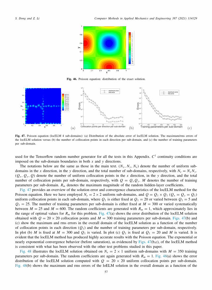
S. Dong and Z. Li Computer Methods in Applied Mechanics and Engineering 387 (2021) 114129
i
bto(oIeni
Fig. 46. Poisson equation: distribution of the exact solution.
Fig. 47. Poisson equation (locELM 4 sub-domains): (a) Distribution of the absolute error of locELM solution. The maximum/rms errors ofthe locELM solution versus (b) the number of collocation points in each direction per sub-domain, and (c) the number of training parametersper sub-domain.
used for the Tensorflow random number generator for all the tests in this Appendix. C1 continuity conditions aremposed on the sub-domain boundaries in both x and y directions.
The notations below are the same as those in the main text. (Nx , Ny, Ne) denote the number of uniform sub-domains in the x direction, in the y direction, and the total number of sub-domains, respectively, with Ne = Nx Ny .(Qx , Q y, Q) denote the number of uniform collocation points in the x direction, in the y direction, and the totalnumber of collocation points per sub-domain, respectively, with Q = Qx Q y . M denotes the number of trainingparameters per sub-domain. Rm denotes the maximum magnitude of the random hidden-layer coefficients.
Fig. 47 provides an overview of the solution error and convergence characteristics of the locELM method for thePoisson equation. Here we have employed Ne = 2× 2 uniform sub-domains, and Q = Q1× Q1 (Qx = Q y = Q1)uniform collocation points in each sub-domain, where Q1 is either fixed at Q1 = 20 or varied between Q1 = 5 andQ1 = 25. The number of training parameters per sub-domain is either fixed at M = 300 or varied systematicallyetween M = 25 and M = 600. The random coefficients are generated with Rm = 1, which approximately lies inhe range of optimal values for Rm for this problem. Fig. 47(a) shows the error distribution of the locELM solutionbtained with Q = 20 × 20 collocation points and M = 300 training parameters per sub-domain. Figs. 47(b) andc) show the maximum and rms errors in the overall domain of the locELM solution as a function of the numberf collocation points in each direction (Q1) and the number of training parameters per sub-domain, respectively.n plot (b) M is fixed at M = 300 and Q1 is varied. In plot (c) Q1 is fixed at Q1 = 20 and M is varied. It isvident that the locELM method has produced highly accurate results with the Poisson equation. The exponential orearly exponential convergence behavior (before saturation), as evidenced by Figs. 47(b,c), of the locELM methods consistent with what has been observed with the other test problems studied in this paper.
Fig. 48 illustrates the locELM solution obtained on Ne = 2 × 1 uniform sub-domains with M = 350 trainingarameters per sub-domain. The random coefficients are again generated with Rm = 1. Fig. 48(a) shows the erroristribution of the locELM solution computed with Q = 20 × 20 uniform collocation points per sub-domain.
ig. 48(b) shows the maximum and rms errors of the loELM solution in the overall domain as a function of the57

S. Dong and Z. Li Computer Methods in Applied Mechanics and Engineering 387 (2021) 114129
e
t(
l
FS
Fig. 48. Poisson equation (locELM 2 sub-domains): (a) Distribution of the absolute error of locELM solution. (b) The maximum/rms errorsof the locELM solution, and (c) the training time, versus the number of collocation points in each direction per sub-domain.
Fig. 49. Poisson equation (FEM, linear elements): (a) FEM error distribution computed on a 1000 × 1000 mesh. (b) The FEM maximum/rmsrrors in the domain, and (c) the FEM computation time, as a function of the number of elements in each direction. An N × N mesh
contains 2N 2 triangular linear elements.
Fig. 50. Poisson equation: The maximum error of the locELM/FEM solutions versus the training/computation time. The locELM datacorrespond to those of Figs. 48(b,c) with 2 sub-domains, where the number of collocation points is varied. The FEM data correspond tothose of Figs. 49(b,c), where the number of elements in the mesh is varied.
number of uniform collocation points in each direction Q1 (with Qx = Q y = Q1) per sub-domain. Fig. 48(c) showshe corresponding network training time as a function of Q1. We can observe the exponential decrease of the errorsbefore saturation), and the near-linear growth of the training time, with increasing number of collocation points.
We next compare these locELM simulation results with those of the classical finite element method (2nd-order,inear elements) with Figs. 49 and 50 and Table 11. The setting for the FEM simulations is as follows. We employ aN1×N2 uniform rectangular mesh in the FEM simulation, where N1 and N2 are specified below. As stipulated by theEniCS library, each rectangle in the mesh is further divided along its diagonal into two triangular linear elements.
o an N1 × N2 rectangular mesh contains a total of 2N1 N2 triangular linear elements for the FEM simulations.58

S. Dong and Z. Li Computer Methods in Applied Mechanics and Engineering 387 (2021) 114129
dsawTq
tooocidotutoaTaow
Table 11Poisson equation: Comparison between locELM and the classical FEM (linear elements) in terms of the maximum/rms errors in the domainand the training or computation time. The FEM results correspond to those of Fig. 49. The locELM results correspond to those of Fig. 48for 2 sub-domains and those of Fig. 47 for 4 sub-domains. Q and M denote the number of uniform collocation points and the number oftraining parameters per sub-domain, respectively.
Method Mesh Sub-domains Q M Max-error rms-error Wall-time(seconds)
FEM 250 × 250 – – – 4.41e − 4 1.24e − 4 0.70400 × 400 – – – 1.72e − 4 4.83e − 5 1.87500 × 500 – – – 1.10e − 4 3.09e − 5 3.09600 × 600 – – – 7.66e − 5 2.15e − 5 4.76700 × 700 – – – 5.63e − 5 1.58e − 5 6.83800 × 800 – – – 4.31e − 5 1.21e − 5 9.01900 × 900 – – – 3.41e − 5 9.54e − 6 12.31000 × 1000 – – – 2.76e − 5 7.73e − 6 16.2
locELM – 2 5 × 5 350 1.73e − 1 3.69e − 2 5.2– 2 8 × 8 350 3.26e − 3 5.02e − 4 5.6– 2 10 × 10 350 2.16e − 4 4.78e − 5 5.7– 2 12 × 12 350 6.72e − 5 1.52e − 5 6.4– 2 15 × 15 350 1.03e − 6 2.34e − 7 7.1– 2 20 × 20 350 1.45e − 8 1.35e − 9 8.6– 2 25 × 25 350 2.81e − 8 1.98e − 9 10.4
– 4 5 × 5 300 1.41e − 1 3.01e − 2 9.8– 4 8 × 8 300 7.56e − 4 1.45e − 4 10.1– 4 10 × 10 300 1.90e − 4 4.21e − 5 11.1– 4 12 × 12 300 1.37e − 5 3.29e − 6 12.2– 4 15 × 15 300 1.20e − 7 2.80e − 8 13.6– 4 20 × 20 300 6.57e − 9 4.49e − 10 17.9– 4 25 × 25 300 6.72e − 9 5.21e − 10 20.8
Fig. 49 provides an overview of the FEM simulation results of the Poisson equation. Fig. 49(a) shows theistribution of the absolute error of the FEM solution obtained on a 1000 × 1000 mesh, indicating that the FEMolution is quite accurate. Figs. 49(b) and (c) show the maximum/rms errors of the FEM solution in the domain,nd the FEM computation time, as a function of the number of elements in each direction of the mesh (N1). Heree have varied N1 systematically between N1 = 25 and N1 = 1000, while maintaining N1 = N2 in the mesh.he second-order convergence rate can be clearly observed from Fig. 49(b). The computation time approximatelyuadruples as the number of elements in each direction (N1) doubles.
In Fig. 50 we plot the maximum error in the domain of the locELM solution (and the FEM solution) versushe network-training time (respectively the FEM computation time). Here the locELM data correspond to thosef Fig. 48(b,c), with Ne = 2 × 1 sub-domains, M = 350 training parameters per sub-domain, and the numberf collocation points per sub-domain varied between 5 × 5 and 25 × 25. The FEM data correspond to thosef Figs. 49(b,c), with the mesh size varied between 25 × 25 and 1000 × 1000. We observe that the accuracy-ost relation for the current locELM method and the classical FEM is qualitatively different. With FEM, the errornitially decreases rapidly with increasing computation time (smaller mesh), and then the error reduction slows downramatically with respect to the computation time (larger mesh). When the mesh size becomes moderate or large,nly slight improvement in the accuracy can be gained with increasing computation time for the classical FEM. Onhe other hand, with locELM the error decreases approximately exponentially with increasing computation time,ntil it saturates at a certain level and no longer decreases as the computation time further increases. Fig. 50 showshat there is a crossover point, below which the FEM outperforms the locELM and beyond which the locELMutperforms the FEM. By saying one method outperforming the other, we mean that the first method can achievebetter accuracy with the same computation time, or can achieve the same accuracy with less computation time.his suggests that with a smaller FEM mesh (or a smaller number of training data points for locELM) the FEM canchieve a better accuracy than locELM with the same computation time. On the other hand, with a larger numberf training data points (or a larger mesh for FEM) the locELM can achieve a better accuracy than the classical FEM
ith the same computation time.59

S. Dong and Z. Li Computer Methods in Applied Mechanics and Engineering 387 (2021) 114129
Fig. 51. Poisson equation (comparing locELM with higher-order FEM): The FEM maximum/rms errors (a) and the computation time (b)as a function of the number of elements in each direction, obtained with Lagrange elements of degree 3. The locELM maximum/rms errors(c) and the network training time (d) as a function of the number of collocation points in each direction per sub-domain, obtained withNe = 2× 2 = 4 uniform sub-domains (M = 325 and Rm = 1).
Table 11 provides more concrete error and computation time data for comparison between locELM and theclassical FEM for the Poisson equation. Here we list the maximum and rms errors of the locELM and FEM solutions,as well as the locELM training time and FEM computation time, corresponding to a set of FEM meshes and locELMresolutions. The locELM data include those obtained on both two and four sub-domains. One can observe that theFEM errors and computation time on the 700 × 700 mesh are comparable to those of the locELM method with 2sub-domains and 12 × 12 collocation points per sub-domain. With simulation resolutions below these values theclassical FEM outperforms locELM, and with resolutions above these values the locELM outperforms the classicalFEM. It can also be observed that the FEM errors and computation time on the 900 × 900 mesh are comparableto those of the locELM method with 4 sub-domains and 12 × 12 collocation points per sub-domain. The classicalFEM outperforms the locELM with resolutions below these values, and the locELM method outperforms the FEMwith resolutions beyond these values.
In all the foregoing comparisons we have used the classical finite element method, i.e. second-order with linearelements. We next provide some comparisons between the locELM method and the FEM with higher-order elements,specifically with higher-order Lagrange elements [54], which are available from the FEniCS library. The simulationresults and the comparison are summarized in Figs. 51 and 52.
Figs. 51(a) and (b) show the maximum/rms errors of the FEM solution obtained with Lagrange elements ofdegree 3 (4th-order), as well as the computation time, as a function of the number of elements in each direction.Here the size of the rectangular mesh is varied systematically between 10 × 10 and 350 × 350. One can clearlyobserve the 4th-order convergence rate and the rapid growth in the computation time as the number of elementsin the mesh increases. Figs. 51(c) and (d) show the maximum/rms errors of the locELM solution, and the networktraining time, as a function of the number of collocation points in each direction per sub-domain. Here we haveemployed Ne = 2× 2 uniform sub-domains, M = 325 training parameters per sub-domain, Rm = 1 for generatingthe random coefficients, and Q = Q1 × Q1 collocation points per sub-domain with Q1 varied systematically. Wecan observe the exponential decrease in the locELM errors (before saturation) and the near-linear growth in thenetwork training time.
60

S. Dong and Z. Li Computer Methods in Applied Mechanics and Engineering 387 (2021) 114129
so
a
FrLcLltad
cfiFAptai
R
Fig. 52. Poisson equation (comparing locELM with higher-order FEM): The maximum error in the domain versus the training/computationtime for locELM and higher-order FEM. The FEM results are obtained with Lagrange elements of degrees 3 and 4, with the degree-3FEM results corresponding to those of Figs. 51(a,b). The locELM results are obtained with Ne = 2 (M = 350) and Ne = 4 (M = 325)ub-domains, with the two-subdomain results corresponding to those of Figs. 48(b,c) and the four-subdomain results corresponding to thosef Figs. 51(c,d).
In Fig. 52 we plot the maximum error in the domain of the locELM solution and the higher-order FEM solution,s a function of the training/computation time. The locELM data include those with 2 sub-domains (M = 350,
Q varied) corresponding to Figs. 48(b,c) and those with 4 sub-domains (M = 325, Q varied) corresponding toigs. 51(c,d). The FEM data include those obtained with Lagrange elements of degree 3 and degree 4. The FEMesults with degree-three Lagrange elements correspond to those of Figs. 51(a,b). The FEM results with degree-fouragrange elements are obtained with the mesh size varied between 10 × 10 and 160 × 160. Due to the limitedomputer memory, the 160 × 160 mesh is the largest one we can perform the FEM simulations on using theagrange elements of degree 4. Fig. 52 shows that the FEM with degree-three Lagrange elements outperforms the
ocELM using two sub-domains as tested here. There is a crossover point between the degree-three FEM curve andhe locELM curve with four sub-domains. With lower resolutions the degree-three FEM outperforms the locELM,nd with higher resolutions the locELM with four sub-domains outperforms the degree-three FEM. The FEM withegree-four Lagrange elements appear to outperform the locELM in all the cases tested here.
To summarize, as the number of training data points (respectively the number of elements) increases, theonvergence behavior of the locELM method is fundamentally different from that of the classical (second-order)nite element method. When the number of elements (or the number of training data points) is small, the classicalEM outperforms locELM, in the sense it can achieve a better accuracy with the same computation/training time.s the number of elements (or number of training data points) increases, there is a crossover point. Beyond thisoint the locELM outperforms the classical FEM, and achieves a better accuracy with the same training/computationime. Compared with the finite element method employing higher-order elements, the current locELM method islso competitive to a certain degree. But overall it appears not as efficient as the latter in its current state (or perhapsmplementation).
eferences
[1] I. Goodfellow, Y. Bengio, A. Courville, Deep Learning, The MIT Press, 2016.[2] K. Hornik, M. Stinchcombe, H. White, Multilayer feedforward networks are universal approximators, Neural Netw. 2 (1989) 359–366.[3] K. Hornik, M. Stinchcombe, H. White, Universal approximation of an unknown mapping and its derivatives using multilayer feedforward
networks, Neural Netw. 3 (1990) 551–560.[4] N.E. Cotter, The Stone-Weierstrass theorem and its application to neural networks, IEEE Trans. Neural Netw. 4 (1990) 290–295.[5] X. Li, Simultaneous approximations of mulvariate functions and their derivatives by neural networks with one hidden layer,
Neurocomputiing 12 (1996) 327–343.[6] P.J. Werbos, Beyond Regression: New Tools for Prediction and Alaysis in the Behavioral Sciences (Ph.D. thesis), Cambridge, MA,
1974,[7] S. Haykin, Neural Networks: A Comprehensive Foundation, Prentice Hall, 1999.[8] J. Sirignano, K. Spoliopoulos, DGM: A deep learning algorithm for solving partial differential equations, J. Comput. Phys. 375 (2018)
1339–1364.
61

S. Dong and Z. Li Computer Methods in Applied Mechanics and Engineering 387 (2021) 114129
[9] M. Raissi, P. Perdikaris, G.E. Karniadakis, Physics-informed neural networks: a deep learning framework for solving forward andinverse problems involving nonlinear partial differential equations, J. Comput. Phys. 378 (2019) 686–707.
[10] I.E. Lagaris, A.C. Likas, D.I. Fotiadis, Artificial neural networks for solving ordinary and partial differential equations, IEEE Trans.Neural Netw. 9 (1998) 987–1000.
[11] I.E. Lagaris, A.C. Likas, D.G. Papageorgiou, Neural-network methods for boundary value problems with irregular boundaries, IEEETrans. Neural Netw. 11 (2000) 1041–1049.
[12] K. Rudd, S. Ferrari, A constrained integration (CINT) approach to solving partial differential equations using artificial neural networks,Neurocomputing 155 (2015) 277–285.
[13] W. E, B. Yu, The deep Ritz method: a deep learning-based numerical algorithm for solving variational problems, Commun. Math.Stat. 6 (2018) 1–12.
[14] N. Winovich, K. Ramani, G. Lin, ConvPDE-UQ: Convolutional neural networks with quantified uncertainty for heterogeneous ellipticpartial differential equations on varied domains, J. Comput. Phys. 394 (2019) 263–279.
[15] J. He, J. Xu, Mgnet: A unified framework for multigrid and convolutional neural network, Sci. China Math. 62 (2019) 1331–1354.[16] W. Xing, R.M. Kirby, S. Zhe, Deep corgionalization for the emulation of spatial-temporal fields, 2019, ArXiv:1910.07577.[17] Y. Zang, G. Bao, X. Ye, H. Zhou, Weak adversarial networks for high-dimensional partial differential equations, J. Comput. Phys. 411
(2020) 109409.[18] Y. Wang G. Lin, Efficient deep learning techniques for multiphase flow simulation in heterogeneous porous media, J. Comput. Phys.
401 (2020) 108968.[19] E. Samanaiego, C. Anitescu, S. Goswami, V.M. Nguyen-Thanh, H. Guo, K. Hamdia, X. Zhuang, T. Rabczuk, An energy approach to the
solution of partial differential equations in computational mechanics via machine learning: concepts, implementation and applications,Comput. Methods Appl. Mech. Engrg. 362 (2020) 112790.
[20] J. Xu, The finite neuron method and convergence analysis, 2020, ArXiv:2010.01458.[21] A.G. Baydin, B.A. Pearlmutter, A.A. Radul, J.M. Siskind, Automatic differentiation in machine learning: a survey, J. Mach. Learn.
Res. 18 (2018) 1–43.[22] A.D. Jagtap, E. Kharazmi, G.E. Karniadakis, Conservative physics-informed neural networks on discrete domains for conservation laws:
applications to forward and inverse problems, Comput. Methods Appl. Mech. Engrg. 365 (2020) 113028.[23] G.-B. Huang, Q.-Y. Zhu, C.-K. Siew, Extreme learning machine: theory and applications, Neurocomputing 70 (2006) 489–501.[24] G.-B. Huang, D.H. Wang, Y. Lan, Extreme learning machines: a survey, Int. J. Mach. Learn. Cybern. 2 (2011) 107–122.[25] G.H. Golub, C.F.V. Loan, Matrix Computations, third ed., Johns Hopkins Press, MD, 1996.[26] Y.H. Pao, G.H. Park, D.J. Sobajic, Learning and generalization characteristics of the random vector functional-link net, Neurocomputing
6 (1994) 163–180.[27] B. Igelnik, Y.H. Pao, Stochastic choice of basis functions in adaptive function approximation and the functional-link net, IEEE Trans.
Neural Netw. 6 (1995) 1320–1329.[28] W. Maass, H. Markram, On the computational power of recurrent circuits of spiking neurons, J. Comput. System Sci. 69 (2004)
593–616.[29] H. Jaeger, M. Lukosevicius, D. Popovici, U. Siewert, Optimization and applications of echo state networks with leaky integrator
neurons, Neural Netw. 20 (2007) 335–352.[30] L. Zhang, P.N. Suganthan, A comprehensive evaluation of random vector functional link networks, Inform. Sci. 367–368 (2016)
1094–1105.[31] C.S. Webster, Alan Turing’s unorganized machines and artificial neural networks: his remarkable early work and future possibilities,
Evol. Intel. 5 (2012) 35–43.[32] F. Rosenblatt, The perceptron: a probabilistic model for information storage and organization in the brain, Psychol. Rev. 65 (1958)
386–408.[33] S. Balasundaram, Kapil, Application of error minimized extreme learning machine for simultaneous learning of a function and its
derivativs, Neurocomputing 74 (2011) 2511–2519.[34] Y. Yang, M. Hou, J. Luo, A novel improved extreme learning machine algorithm in solving ordinary differential equations by Legendre
neural network methods, Adv. Differential Equations 469 (2018) 1–24.[35] H. Sun, M. Hou, Y. Yang, T. Zhang, F. Weng, F. Han, Solving partial differential equations based on Bernsteirn neural network and
extreme learning machine algorithm, Neural Process. Lett. 50 (2019) 1153–1172.[36] S. Panghal, M. Kumar, Optimization free neural network approach for solving ordinary and partial differential equations, Eng. Comput.
(2020) Early Access.[37] H. Liu, B. Xing, Z. Wang, L. Li, Legendre neural network method for several classes of singularly perturbed differential equations
based on mapping and piecewise optimization technology, Neural Process. Lett. 51 (2020) 2891–2913.[38] V. Dwivedi, B. Srinivasan, Physics informed extreme learning machine (PIELM) − a rapid method for the numerical solution of partial
differential equations, Neurocomputing 391 (2020) 96–118.[39] Barry F. Smith, Petter E. Bjø rstad, William D. Gropp, Domain Decomposition: Parallel Multilevel Methods for Elliptic Partial
Differential Equations, Cambridge University Press, 1996.[40] A. Toselli, O. Widlund, Domain Decomposition Methods − Algorithms and Theory, Springer, 2005.[41] S. Dong, BDF-like methods for nonlinear dynamic analysis, J. Comput. Phys. 229 (2010) 3019–3045.[42] S. Dong, J. Shen, A pressure correction scheme for generalized form of energy-stable open boundary conditions for incompressible
flows, J. Comput. Phys. 291 (2015) 254–278.[43] S. Dong, Multiphase flows of N immiscible incompressible fluids: a reduction-consistent and thermodynamically-consistent formulation
and associated algorithm, J. Comput. Phys. 361 (2018) 1–49.
62

S. Dong and Z. Li Computer Methods in Applied Mechanics and Engineering 387 (2021) 114129
[44] K. Li, K. Tang, T. Wu, Q. Liao, D3M: A deep domain decomposition method for partial differential equations, IEEE Access 8 (2020)5283–5294.
[45] G.E. Karniadakis, S.J. Sherwin, Spectral/Hp Element Methods for Computational Fluid Dynamics, second ed., Oxford University Press,2005.
[46] Y. Yu, R.M. Kirby, G.E. Karniadakis, Spectral element and hp methods, Encycl. Comput. Mech. 1 (2017) 1–43.[47] X. Zheng, S. Dong, An eigen-based high-order expansion basis for structured spectral elements, J. Comput. Phys. 230 (2011) 8573–8602.[48] S. Dong, Z. Yosibash, A parallel spectral element method for dynamic three-dimensional nonlinear elasticity problems, Comput. Struct.
87 (2009) 59–72.[49] S. Dong, J. Shen, A time-stepping scheme involving constant coefficient matrices for phase field simulations of two-phase incompressible
flows with large density ratios, J. Comput. Phys. 231 (2012) 5788–5804.[50] D.P. Kingma, J. Ba, Adam: a method for stochastic optimization, 2014, ArXiv:1412.6980.[51] J. Nocedal, S.J. Wright, Numerical Optimization, second ed., Springer, 2006.[52] H.P. Langtangen, A. Logg, Solving PDEs in Python, the FEniCS Tutorial I, SpringerOpen, 2016.[53] S. Dong, N. Ni, A method for representing periodic functions and enforcing exactly periodic boundary conditions with deep neural
networks, J. Comput. Phys. 435 (2021) 110242.[54] R.L. Courant, Variational methods for the solution of problems of equilibrium and vibration, Bull. Amer. Math. Soc. 49 (1943) 1–23.
63