HAL Id: hal-01617692https://hal.inria.fr/hal-01617692

Submitted on 18 May 2018

HAL is a multi-disciplinary open accessarchive for the deposit and dissemination of sci-entific research documents, whether they are pub-lished or not. The documents may come fromteaching and research institutions in France orabroad, or from public or private research centers.

L’archive ouverte pluridisciplinaire HAL, estdestinée au dépôt et à la diffusion de documentsscientifiques de niveau recherche, publiés ou non,émanant des établissements d’enseignement et derecherche français ou étrangers, des laboratoirespublics ou privés.

A Schwarz-based domain decomposition method for thedispersion equation

Joao Guilherme Caldas Steinstraesser, Rodrigo Cienfuegos, José Daniel GalazMora, Antoine Rousseau

To cite this version:Joao Guilherme Caldas Steinstraesser, Rodrigo Cienfuegos, José Daniel Galaz Mora, AntoineRousseau. A Schwarz-based domain decomposition method for the dispersion equation. Journalof Applied Analysis and Computation, Wilmington Scientific Publisher, 2018. hal-01617692

A Schwarz-based domain decomposition method for thedispersion equation

Joao Guilherme Caldas Steinstraessera,∗, Rodrigo Cienfuegosb, Jose DanielGalaz Morab, Antoine Rousseauc

a MERIC, Marine Energy Research & Innovation Center, Avda. Apoquindo 2827,Santiago, Chile

bDepartamento de Ingenierıa Hidraulica y Ambiental, Pontificia Universidad Catolica deChile, Av. Vicuna Mackenna 4680 - Macul, Santiago, Chile

cInria and Inria Chile, Avda. Apoquindo 2827, Santiago, Chile

Abstract

We propose a Schwarz-based domain decomposition method for solving a dis-persion equation consisting on the linearized KdV equation without the ad-vective term, using simple interface operators based on the exact transparentboundary conditions for this equation. An optimization process is performedfor obtaining the approximation that provides the method with the fastest con-vergence to the solution of the monodomain problem.

Keywords: domain decomposition method, Schwarz method, transparentboundary conditions, KdV equation

1. Introduction

The Korteweg - de Vries (KdV) equation, derived by [11] in 1895, modelsthe propagation of waves with small amplitude and large wavelength, taking inaccount nonlinear and dispersive effects. In terms of dimensionless but unscaledvariables, it can be written as [2]

ut + ux + uux + uxxx = 0

As done in [14] (and in [3] as a special case of their work), we will focus inthis paper on the linearized KdV equation without the advective term :

ut + uxxx = 0 (1)

to which we will refer as dispersion equation.

∗Corresponding authorEmail addresses: joao.caldas@meric.cl (Joao Guilherme Caldas Steinstraesser),

racienfu@ing.puc.cl (Rodrigo Cienfuegos), jdgalaz@uc.cl (Jose Daniel Galaz Mora),antoine.rousseau@inria.fr (Antoine Rousseau)

Preprint submitted to Elsevier October 16, 2017

The work developed here is inspired from [14] and [3]. Nevertheless, ourobjectives are different from theirs. In this paper we propose an additive Schwarzmethod (ASM) for solving the dispersion equation (1) in a bounded domain,i.e., we decompose the computational domain in subdomains and solve the time-dependent problem in each one of them. Our work focuses on the formulation ofappropriate and optimized conditions on the interface between the subdomains,in order to minimize the error due to the domain decomposition method (DDM)and to accelerate the convergence of the method.

The interface boundary conditions (IBCs) proposed here are based on theexact transparent boundary conditions (TBCs) for the equation (1), derived by[14] and [3]. The TBCs make the approximate solution in the computationaldomain coincide with the solution of the whole domain, but its exact computa-tion is not doable in general [1]. [14] and [3] proposed numerical approximationsfor these conditions, seeking to reduce the error created by the introduction ofartificial boundaries.

In the work presented here, we do not propose approximate TBCs for re-ducing the error related to the finitude of the computational domain. In fact,we intend to reduce the error created by the decomposition of the domain andthe introduction of an artificial interface boundary condition, in the context ofa DDM. In other words, we study the effectiveness of the boundary conditionsas IBCs, not as TBCs. As a consequence, our work shall not use the same ref-erence solution as the one used by [14] and [3]: for validating their approaches,they compare their approximate solution with the exact solution in the wholedomain. On the other hand, our reference solution is the approximate solutioncomputed on the computational monodomain. Moreover, in order to isolate theerror due to the DDM from that originated by time discretization, we study ourmethod locally in time, i.e., along one time step.

This paper is organized as follows : In Section 2, we describe the DDM usedhere and we recall the exact TBCs derived by [14] for equation (1). Then, wepropose approximations for them, leading to very simple mixed-type conditions(avoiding, for example, integrations in time) to be used as IBCs in the DDM.Small modifications are proposed for these IBCs such that the solution of theDDM problem converges exactly to the reference solution (the solution of themonodomain problem). In Section 3, we perform a large set of numerical testsin order to optimize the IBCs, in the sense that we search the coefficients thatprovide the fastest convergence for the DDM iterative process.

2. Resolution of the dispersion equation using a domain decomposi-tion method

We propose in this section a DDM for solving the problem

2

ut + uxxx = 0, x ∈ Ω, t ≥ t0u(t0, x) = uexact(t0, x), x ∈ Ω

Υ1(u,−L) = 0, t ≥ t0Υ2(u, L) = 0, t ≥ t0Υ3(u, L) = 0, t ≥ t0

(2)

in the domain Ω = [a, b].We firstly present a brief review of the DDM considered here, the parallel

or additive Schwarz method (ASM) and then we propose IBCs for applying itto the problem solved in this paper.

2.1. The Schwarz Method

Domain decomposition methods allow to decompose a domain Ω in multi-ple subdomains Ωi (that can possibly overlap) and solve the problem in eachone of them. Therefore, one must find functions that satisfy the PDE in eachsubdomain and that match on the interfaces.

The first DDM developed was the alternating or multiplicative Schwarzmethod, in which the IBCs for computing the solution in a subdomain arefunction of the most updated solution in the neighbor subdomains. We con-sider here a modified version of this algorithm, introduced more recently by [12]and known as parallel or additive Schwarz method. In this algorithm, the IBCsfor computing the solution uki , in the subdomain Ωi and iteration k, are alwaysconstructed using the solution uk−1

j , j 6= i, of the previous iteration in theneighbor subdomains.

This modification originates an inherently parallel algorithm, which one nat-urally implements with parallel computing. The advantages obtained with theparallelism become more evident when the number of subdomains increases [12].

In the ASM, the boundary condition for the problem in Ωi, in each interfacebetween the subdomains Ωi and Ωj , can be written as

Bi(uk+1i ) = Bi(ukj ) (3)

where (3), Bi denotes the operator of the IBC. This operator allows the con-struction of more general Schwarz methods: in the original one, the IBCs areDirichlet conditions (i.e., Bi(u) = u ) [10, 13].

Without loss of generality, in the following we consider a domain Ω decom-posed in two non-overlapping subdomains, Ω1 and Ω2, with Γ = Ω1

⋂Ω2.

When implementing a Schwarz method, one must define appropriate opera-tors Bi such that:

• There is a unique solution ui in each subdomain Ωi;

• The solution ui in each subdomain Ωi converges to u|Ωi, i.e., the solution

u, restricted to Ωi, of the problem in the monodomain Ω;

3

Moreover, one wants the method to show a fast convergence.In fact, accordingly to [10], the optimal additive Schwarz method for solving

the problem A(u) = f in Ω

u = 0 on ∂Ω

where A is a partial differential operator, is the one which uses as IBCs theexact TBCs for the problem, which are given by

Bi(u) =∂

∂niu+D2N(u)

where ∂ni is the outward normal to Ωi on Γ , and the D2N (Dirichlet toNeumann) operator is defined by

D2N : α(x) 7→ ∂

∂nciv

∣∣∣∣Γ

with α defined on Γ. v is solution of the following problem, solved in thecomplementary set of Ωi, denoted by Ωci

A(v) = f in Ωciv = 0 on ∂Ωi\Γv = α on Γ

The ASM using such exact TBCs is optimal in the sense that it converges intwo iterations, and no other ASM can converge faster [10]. Nevertheless, theseTBCs, in general, are not simple to compute both analytically and numerically.More specifically, they are nonlocal in time, so they must be approximated foran efficient numerical implementation [1]. These facts motivate us to look forsimpler operators to use as IBCs in the ASM. We propose them based on theexact TBCs operators for the equation (1), as derived by [3].

2.2. Interface boundary condition operators based on the exact TBCs for thedispersion equation

In [3], TBCs are derived for the one-dimensional continuous linearized KdVequation (or Airy equation):

ut + U1ux + U2uxxx = h(t, x), t ∈ R+, x ∈ R (4)

where U1 ∈ R, U2 ∈ R+∗ and h is a source term, assumed to be compactly

supported in a finite computational domain [a, b], a < b.For the homogeneous initial boundary value problem

ut + U1ux + U2uxxx = 0, t ∈ R+, x ∈ [a, b]

u(0, x) = u0(x), x ∈ [a, b]

+boundary conditions

4

the TBCs are given by [3, equations (2.17) -(2.18)]

u(t, a)− U2L−1

(λ1(s)2

s

)∗ ux(t, a)− U2L−1

(λ1(s)

s

)∗ uxx(t, a) = 0

u(t, b)− L−1

(1

λ1(s)2

)∗ uxx(t, b) = 0

ux(t, b)− L−1

(1

λ1(s)

)∗ uxx(t, b) = 0

(5)

where L−1 denotes the inverse Laplace transform, ∗ the convolution operator,s ∈ C, Re(s) > 0, is the Laplace frequency and λ1 is, among the three roots ofthe cubic characteristic equation obtained when solving (4) in the Laplace spaceand in the complementary set of [a, b], the only one with negative real part.

In this paper, we focus on the special case U1 = 0, U2 = 1, which results onthe dispersion equation (1). In this case, accordingly to [14], the only root withnegative real part is

λ(s) = λ1(s) = − 3√s (6)

The computation of the TBCs (5) is not simple due to the inverse Laplacetransform, which makes these conditions nonlocal in time. Therefore, we pro-pose approximations of the root (6) that avoid integrations in time, making theoperators considerably simpler.

Obviously, we do not expect these operators to be as accurate as the ap-proximate TBCs proposed by [3] (who derives TBCs for the discrete linearizedKdV equation). Nevertheless, the objectives of our work and the work of [3]are very different: while they seek to minimize the error of the computed solu-tion (compared to the analytical one) due to the boundary conditions, we wanthere to apply our operators as IBCs in a DDM. Therefore, our objective layson the convergence of the DDM to the solution of the same problem in themonodomain, independently of the errors on the external boundaries.

We use the constant polynomial P0(s) = c for approximating λ2/s (whichcan be seen as a (0,0) order Pade approximation). Moreover, as a consequenceof (6), we can approximate the other operands of the inverse Laplace transformsin (5) only in function of c :

λ2

s= c,

λ

s= −c2, 1

λ(s)2= c2,

1

λ(s)= −c (7)

Replacing (7) in (5), using some well-know properties of the Laplace Trans-form (linearity and convolution) , we get the approximate transparent boundaryconditions

Θc1(u, x) = u(t, x)− cux(t, x) + c2uxx(t, x) = 0

Θc2(u, x) = u(t, x)− c2uxx(t, x) = 0

Θc3(u, x) = ux(t, x) + cuxx(t, x) = 0

(8)

5

We notice that the approximation (8) has the same form as the exact TBCsfor the equation (1) presented in [14] and [3], being the constant c an approxi-mation for fractional integral operators.

We also remark that (8) are mixed-type boundary conditions (up to thesecond derivative of the solution), which, in the next section, we apply as IBCsin a DDM and we seek to optimize in order to accelerate the convergence ofthis method. The idea of using optimized boundary conditions in DDMs wasalready explored in [9] and [4], in the context of the Schrodinger equation.

Considering a discrete domain with mesh size ∆x and points x0, ..., xN andusing some finite difference approximations, the operators (8) are discretized as

u0 − cu1 − u0

∆x+ c2

u0 − 2u1 + u2

∆x2= 0

uN − c2uN − 2uN−1 + uN−2

∆x2= 0

uN − uN−1

∆x+ c

uN − 2uN−1 + uN−2

∆x2= 0

(9)

2.3. ASM with the proposed IBCs

With the operators Θci defined, we now apply them in a DDM, with two non-

overlapping subdomains Ω1 = [a, 0] and Ω2 = [0, b], a < 0 < b and interfaceΓ = Ω1 ∩ Ω2

Considering that we want to analyze and minimize the error due to the ap-plication of a DDM (isolating it from the error acumulated along the time steps,due to the temporal discretization), the reference solution uref in our study isthe solution of the monodomain problem (2) solved along onte time step (equa-tion 10). Therefore, we implement a DDM to an evolution problem discretizedin time (thus consisting in an ODE in space), an idea already explored by [5].

u(t0+∆t)−u(t0)∆t + uxxx = 0, x ∈ Ω

u(t0, x) = uexact(t0, x), x ∈ Ω

Υ1(u(t0 + ∆t), a) = 0

Υ2(u(t0 + ∆t), b) = 0

Υ3(u(t0 + ∆t), b) = 0

(10)

The external BCs Υi, i = 1, 2, 3 (i.e., defined on ∂Ωi\Γ) are independentof the interface BCs. Here, we consider Υ1 = Θc=1.0

1 , Υ2 = Θc=0.02 and Υ3 =

Θc=0.03 , which gives

Υ1(u, x) = u− ux + uxx = 0

Υ2(u, x) = u = 0

Υ3(u, x) = ux = 0

This choice was based on the simple form and implementation of theseboundary conditions. Nevertheless, it does not have much importance in thestudy done here, as we want to analyze exclusively the behavior of the DDM. The

6

only restriction for an appropriate study is that the external BCs for computinguref must be the same Υi, i = 1, 2, 3, used for each subdomain in the DDM,as we did in (11)-(12) and (10).

The resolution of the problem (10) by the Additive Schwarz method andusing the IBCs (9) is written as

uk+11 (t0+∆t)−uk+1

1 (t0)∆t + (uk+1

1 )xxx(t0 + ∆t) = 0, x ∈ Ω1

u01(t0) = uexact(t0, x), x ∈ Ω1

Υc1(uk+1

1 (t0 + ∆t), a) = 0,

Θc2(uk+1

1 (t0 + ∆t), 0) = Θc2(uk2(t0 + ∆t), 0),

Θc3(uk+1

1 (t0 + ∆t), 0) = Θc3(uk2(t0 + ∆t), 0)

(11)

uk+12 (t0+∆t)−uk+1

2 (t0)∆t + (uk+1

2 )xxx(t0 + ∆t) = 0, x ∈ Ω2

u02(t0) = uexact(t0, x), x ∈ Ω2

Θc1(uk+1

2 (t0 + ∆t), 0) = Θc1(uk1(t0 + ∆t), 0)

Υc2(uk+1

2 (t0 + ∆t), b) = 0

Υc3(uk+1

2 (t0 + ∆t), b) = 0

(12)

A simple analysis (for example in the Laplace domain) shows that the mon-odomain and DDM problems (10) and (11)-(12) have an unique solution.

We also remark that our proposed DDM can be used for solving the problem(2), i.e., in a time window containing multiple time steps, by solving (11)-(12)in each time step, with the converged solution of the previous time step as initialdata.

Remarks on the notation. In the following study of our proposed DDM, wherewe perform a spatial discretization, we introduce an extra subindex, so thesolution is denoted as uki,j , where i indicates the subdomain Ωi (or, in the caseof the reference solution, i = ref , and in the convergence of the method, i = ∗),j indicates the spatial discrete position and k indicates the iteration.

2.4. Spatial discretization of the problem

Concerning the spatial discretization, the monodomain Ω is divided in 2N+1homogeneously distributed points, numbered from 0 to 2N . In all the analyticaldescription, we consider that the two subdomains Ω1 and Ω2 have the samenumber of points, respectively x0, ..., xN and xN , ..., x2N . The interface pointxN is common to the two domains, having different computed solutions uk1,Nand uk2,N in each one of them. Evidently, we expect, at the convergence of themethod, that u∞1,N = u∞2,N = u∗N

As done in the initial numerical tests in the section 2.2, an implicit FiniteDifference scheme is used here. For the interior points of each one of the do-mains, we consider a second order discretization for the third spatial derivativein equation (1):

7

uk+1i,j − αi,j

∆t+− 1

2uk+1i,j−2 + uk+1

i,j−1 − uk+1i,j+1 + 1

2uk+1i,j+2

∆x3= 0 (13)

which is valid for j = 2, ..., N − 2 in the case i = 1; for j = N + 2, ..., 2N − 2in the case i = 2; and for j = 2, ..., 2N − 2 in the case i = ref . In the aboveexpression, αi,j is a given data (for example, the exact or the converged solutionin the previous time step).

For the points near the boundaries, we use second order uncentered dis-cretizations or the appropriate boundary condition. Considering that one bound-ary condition is written for the left boundary and two for the right one, we haveto impose an uncentered discretization only for the second leftmost point of thedomain. For example, for the point x1 :

uk+11,1 − α1,1

∆t+− 5

2uk+11,1 + 9uk+1

1,2 − 12uk+11,3 + 7uk+1

1,4 − 32u

k+11,5

∆x3= 0

and similarly to the other points near the boundaries.In the resolution of the problem in Ω1, two IBCs are imposed (corresponding

to Θ2 and Θ3) to the discrete equations for the points xN−1 and xN . On theother hand, in the resolution of the problem in Ω2, only one interface boundarycondition is used (corresponding to Θ1), being imposed to the point xN .

Remark : modification of the reference solution. Even if the DDM with theproposed IBCs is compatible with the monodomain problem (which we will seethat is not the case), the solution of the DDM does not converge exactly touref , for a reason that does not depend on the expression of the IBCs, buton the fact that for each domain we write two boundary conditions in theright boundary and only one on the left boundary. We are using a secondorder centered discretization for the third spatial derivative (which uses a stencilof two points in each side of the central point), implying that we must writean uncentered discretization for the point xN+1 when solving the problem inΩ2. Therefore, this point does not satisfy the same discrete equation as in thereference problem. In order to avoid this incompatibility and allow us to studythe behavior of the DDM, we will modify the discretization for the point uN+1 inthe monodomain problem, using the same second-order uncentered expression :

uk+12,N+1 − α2,N+1

∆t+− 5

2uk+12,N+1 + 9uk+1

2,N+2 − 12uk+12,N+3 + 7uk+1

2,N+4 −32u

k+12,N+5

∆x3= 0

Figure 1 resumes the discretizations imposed to each point in the mon-odomain and the DDM problems, as described above:

8

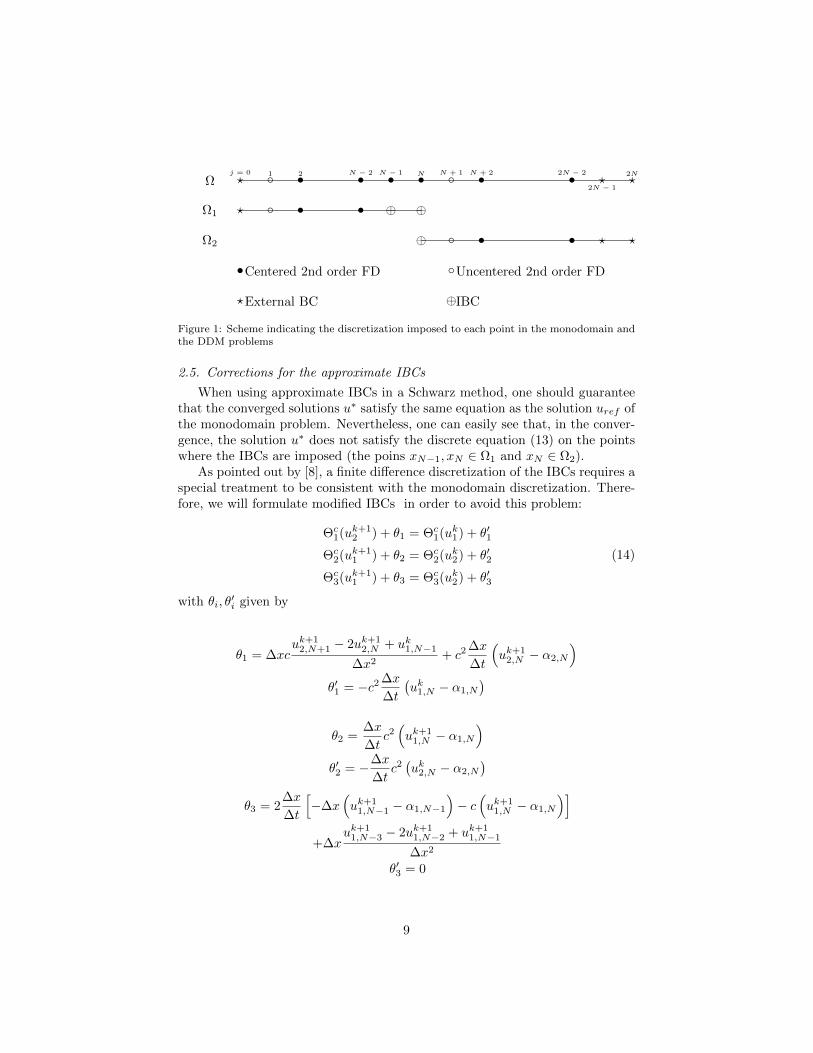
Ωj = 0 1 2 N − 2 N − 1 N N + 1 N + 2 2N − 2

2N − 1

2N? ? ?• • • • • •

Ω1 ? • • ⊕ ⊕

Ω2 ⊕ • • ? ?

•Centered 2nd order FD Uncentered 2nd order FD

?External BC ⊕IBC

Figure 1: Scheme indicating the discretization imposed to each point in the monodomain andthe DDM problems

2.5. Corrections for the approximate IBCs

When using approximate IBCs in a Schwarz method, one should guaranteethat the converged solutions u∗ satisfy the same equation as the solution uref ofthe monodomain problem. Nevertheless, one can easily see that, in the conver-gence, the solution u∗ does not satisfy the discrete equation (13) on the pointswhere the IBCs are imposed (the poins xN−1, xN ∈ Ω1 and xN ∈ Ω2).

As pointed out by [8], a finite difference discretization of the IBCs requires aspecial treatment to be consistent with the monodomain discretization. There-fore, we will formulate modified IBCs in order to avoid this problem:

Θc1(uk+1

2 ) + θ1 = Θc1(uk1) + θ′1

Θc2(uk+1

1 ) + θ2 = Θc2(uk2) + θ′2

Θc3(uk+1

1 ) + θ3 = Θc3(uk2) + θ′3

(14)

with θi, θ′i given by

θ1 = ∆xcuk+1

2,N+1 − 2uk+12,N + uk1,N−1

∆x2+ c2

∆x

∆t

(uk+1

2,N − α2,N

)θ′1 = −c2 ∆x

∆t

(uk1,N − α1,N

)θ2 =

∆x

∆tc2(uk+1

1,N − α1,N

)θ′2 = −∆x

∆tc2(uk2,N − α2,N

)θ3 = 2

∆x

∆t

[−∆x

(uk+1

1,N−1 − α1,N−1

)− c

(uk+1

1,N − α1,N

)]+∆x

uk+11,N−3 − 2uk+1

1,N−2 + uk+11,N−1

∆x2

θ′3 = 0

9

It is straightforward to verify that the DDM problem with these modifica-tions in the IBCs insure that the converged solution u∗ satisfies, in every point,the same discrete equations as the solution uref of the monodomain problem(10).

In addition, we notice that all the modification terms θi, θ′i, i = 1, 2, 3, are

of order O(∆x) (they are composed of discrete versions of time derivatives andsecond spatial derivatives multiplied by ∆x). It is essential to insure that theseterms are small, for the consistency with the approximate IBCs Θi to be fulfilled.

3. Numerical tests for optimizing the IBCs (speed of convergence)

Our objective now is to optimize the IBCs in the sense of minimizing thenumber of iterations of our method until the convergence. We perform a verylarge set of tests in order to find the coefficient c that provide the fastestconvergence. To start with, we make this study with fixed time step and spacestep, in order to analyze exclusively the influence of the coefficient.

As we are interested in the speed with which the solution of the DDM methodconverges to the reference solution, the criteria of convergence used is

eΩ,k ≤ ε

with ε = 10−9 and

eΩ,k = ||uref,N − ukN ||2=

√√√√√∆x

N∑j=0

(uref,j − uk1,j

)2+

2N∑j=N

(uref,j − uk2,j

)2The range of tested coefficients is [−10.0, 20.0] (chosen after initial tests to

identify a proper interval), with a step equal to 0.1 between them (or evensmaller, up to 0.005, in the regions near the optimal coefficients), and the max-imal number of iterations is set to 100.

3.1. Test varying the initial time step and the interface position

As said above, in the first set of tests we consider a fixed time step ∆t =20/2560 = 0.0078125 and a fixed mesh size ∆x = 12/500 = 0.024. Moreover,we consider two subsets of tests, in order to study the speed of convergence withdifferent initial conditions and different sizes of the subdomains:

1. Tests varying the initial time step t0, with the interface in the center ofthe monodomain Ω = [−6, 6];

2. Tests varying the position of the interface (xinterface = −a + α(b − a),where b = −a = 6 and 0 < α < 1), for a fixed initial time t0 = 0.78125.

10

In all the cases, the reference solution uref is the solution of the monodomainproblem (10).

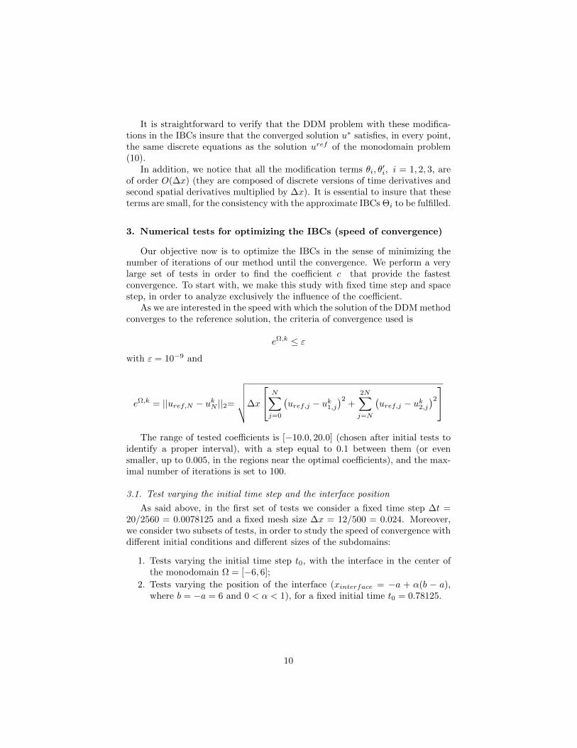
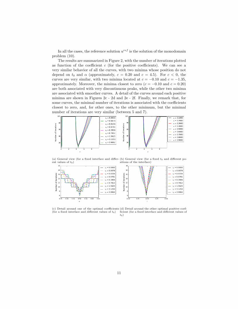
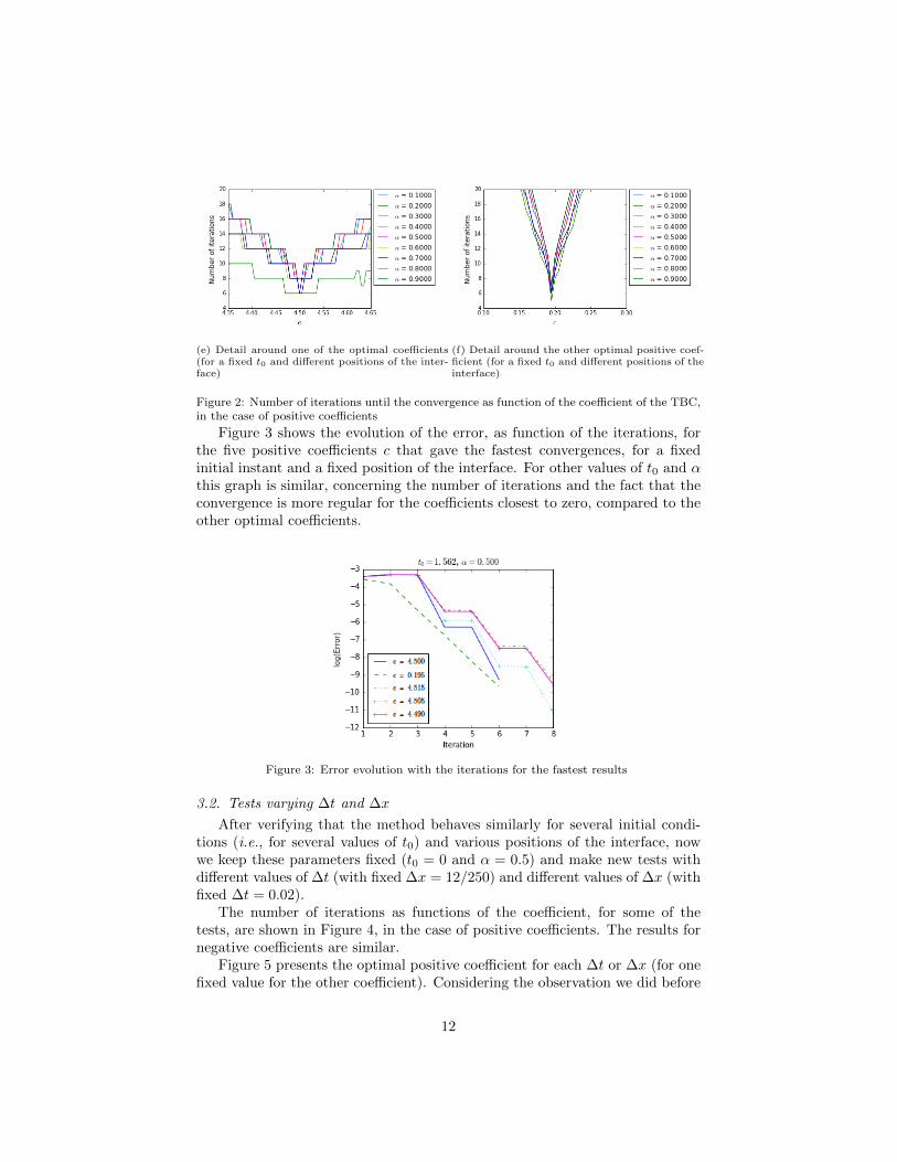
The results are summarized in Figure 2, with the number of iterations plottedas function of the coefficient c (for the positive coefficients). We can see avery similar behavior of all the curves, with two minima whose position do notdepend on t0 and α (approximately, c = 0.20 and c = 4.5). For c < 0, thecurves are very similar, with two minima located at c = −0.10 and c = −1.35,approximately. Moreover, the minima closest to zero (c = −0.10 and c = 0.20)are both associated with very discontinuous peaks, while the other two minimaare associated with smoother curves. A detail of the curves around each positiveminima are shown in Figures 2c - 2d and 2e - 2f. Finally, we remark that, forsome curves, the minimal number of iterations is associated with the coefficientsclosest to zero, and, for other ones, to the other minimum, but the minimalnumber of iterations are very similar (between 5 and 7).

(a) General view (for a fixed interface and differ-ent values of t0)

(b) General view (for a fixed t0 and different po-sitions of the interface)

(c) Detail around one of the optimal coefficients(for a fixed interface and different values of t0)

(d) Detail around the other optimal positive coef-ficient (for a fixed interface and different values oft0)

11

(e) Detail around one of the optimal coefficients(for a fixed t0 and different positions of the inter-face)

(f) Detail around the other optimal positive coef-ficient (for a fixed t0 and different positions of theinterface)

Figure 2: Number of iterations until the convergence as function of the coefficient of the TBC,in the case of positive coefficients

Figure 3 shows the evolution of the error, as function of the iterations, forthe five positive coefficients c that gave the fastest convergences, for a fixedinitial instant and a fixed position of the interface. For other values of t0 and αthis graph is similar, concerning the number of iterations and the fact that theconvergence is more regular for the coefficients closest to zero, compared to theother optimal coefficients.

Figure 3: Error evolution with the iterations for the fastest results

3.2. Tests varying ∆t and ∆x

After verifying that the method behaves similarly for several initial condi-tions (i.e., for several values of t0) and various positions of the interface, nowwe keep these parameters fixed (t0 = 0 and α = 0.5) and make new tests withdifferent values of ∆t (with fixed ∆x = 12/250) and different values of ∆x (withfixed ∆t = 0.02).

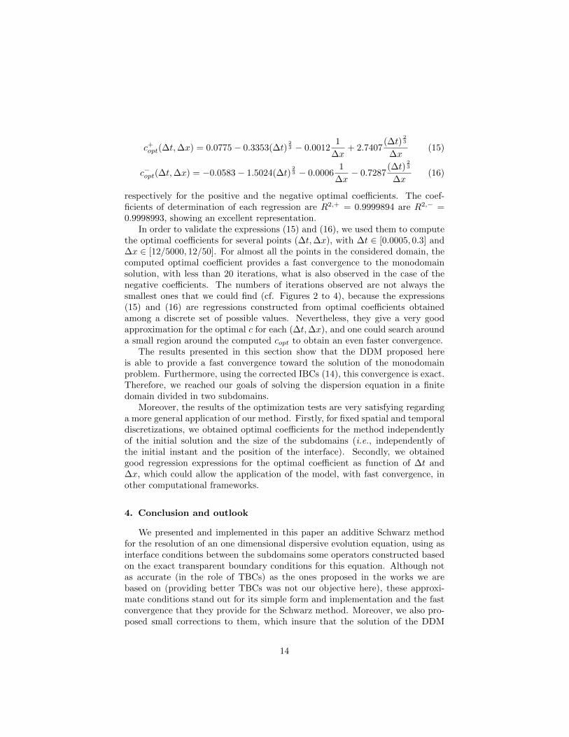
The number of iterations as functions of the coefficient, for some of thetests, are shown in Figure 4, in the case of positive coefficients. The results fornegative coefficients are similar.

Figure 5 presents the optimal positive coefficient for each ∆t or ∆x (for onefixed value for the other coefficient). Considering the observation we did before

12

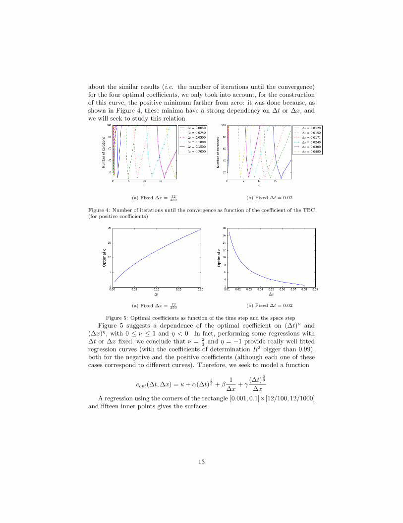
about the similar results (i.e. the number of iterations until the convergence)for the four optimal coefficients, we only took into account, for the constructionof this curve, the positive minimum farther from zero: it was done because, asshown in Figure 4, these minima have a strong dependency on ∆t or ∆x, andwe will seek to study this relation.

(a) Fixed ∆x = 12250

(b) Fixed ∆t = 0.02

Figure 4: Number of iterations until the convergence as function of the coefficient of the TBC(for positive coefficients)

(a) Fixed ∆x = 12250

(b) Fixed ∆t = 0.02

Figure 5: Optimal coefficients as function of the time step and the space step

Figure 5 suggests a dependence of the optimal coefficient on (∆t)ν and(∆x)η, with 0 ≤ ν ≤ 1 and η < 0. In fact, performing some regressions with∆t or ∆x fixed, we conclude that ν = 2

3 and η = −1 provide really well-fittedregression curves (with the coefficients of determination R2 bigger than 0.99),both for the negative and the positive coefficients (although each one of thesecases correspond to different curves). Therefore, we seek to model a function

copt(∆t,∆x) = κ+ α(∆t)23 + β

1

∆x+ γ

(∆t)23

∆x

A regression using the corners of the rectangle [0.001, 0.1]×[12/100, 12/1000]and fifteen inner points gives the surfaces

13

c+opt(∆t,∆x) = 0.0775− 0.3353(∆t)23 − 0.0012

1

∆x+ 2.7407

(∆t)23

∆x(15)

c−opt(∆t,∆x) = −0.0583− 1.5024(∆t)23 − 0.0006

1

∆x− 0.7287

(∆t)23

∆x(16)

respectively for the positive and the negative optimal coefficients. The coef-ficients of determination of each regression are R2,+ = 0.9999894 are R2,− =0.9998993, showing an excellent representation.

In order to validate the expressions (15) and (16), we used them to computethe optimal coefficients for several points (∆t,∆x), with ∆t ∈ [0.0005, 0.3] and∆x ∈ [12/5000, 12/50]. For almost all the points in the considered domain, thecomputed optimal coefficient provides a fast convergence to the monodomainsolution, with less than 20 iterations, what is also observed in the case of thenegative coefficients. The numbers of iterations observed are not always thesmallest ones that we could find (cf. Figures 2 to 4), because the expressions(15) and (16) are regressions constructed from optimal coefficients obtainedamong a discrete set of possible values. Nevertheless, they give a very goodapproximation for the optimal c for each (∆t,∆x), and one could search arounda small region around the computed copt to obtain an even faster convergence.

The results presented in this section show that the DDM proposed hereis able to provide a fast convergence toward the solution of the monodomainproblem. Furthermore, using the corrected IBCs (14), this convergence is exact.Therefore, we reached our goals of solving the dispersion equation in a finitedomain divided in two subdomains.

Moreover, the results of the optimization tests are very satisfying regardinga more general application of our method. Firstly, for fixed spatial and temporaldiscretizations, we obtained optimal coefficients for the method independentlyof the initial solution and the size of the subdomains (i.e., independently ofthe initial instant and the position of the interface). Secondly, we obtainedgood regression expressions for the optimal coefficient as function of ∆t and∆x, which could allow the application of the model, with fast convergence, inother computational frameworks.

4. Conclusion and outlook

We presented and implemented in this paper an additive Schwarz methodfor the resolution of an one dimensional dispersive evolution equation, using asinterface conditions between the subdomains some operators constructed basedon the exact transparent boundary conditions for this equation. Although notas accurate (in the role of TBCs) as the ones proposed in the works we arebased on (providing better TBCs was not our objective here), these approxi-mate conditions stand out for its simple form and implementation and the fastconvergence that they provide for the Schwarz method. Moreover, we also pro-posed small corrections to them, which insure that the solution of the DDM

14

problem converges exactly to the solution of the monodomain problem. Finally,we verified that the speed of convergence depends on the time step, the meshsize and the (only) coefficient for constructing the approximate interface condi-tions; thus, via an optimization process, we obtained and validated regressionexpressions that provide the optimal coefficient (i.e., the one that provides thefastest convergence) in function of ∆t and ∆x.

Natural continuations of the work presented here would be the study of themethod using more complex operators as IBCs, using for example higher-ordersPade approximations for λ2/s and considering different approximations for leftand right boundary conditions. Moreover, we can extend this study for otherproblems, for instance the linearized KdV equation, which adds an advectiveterm on the equation solved here, as well as other models of wave propagation.Finally, we can seek the development of global in time Schwarz methods, usingoptimized Scwharz waveform relaxation methods.

Acknowledgement

This study was conducted under the Marine Energy Research & InnovationCenter (MERIC) project CORFO 14CEI2-28228, and thanks to the support ofinternational partnerships department of Inria, through fundacion Inria Chile.

The authors also want to thank Philippe Bonneton and Veronique Martinfor fruitful discussions related to this work.

References

[1] Antoine, X., Arnold, A., Besse, C., Ehrhardt, M., and Schadle, C. (2008).A review of Transparent Boundary Conditions or linear and nonlinearSchrodinger equations. Commum. Comput. Phys., 4(4):729–796.

[2] Benjamin, T. B., Bona, J. L., and Mahony, J. J. (1972). Model equa-tions for long waves in nonlinear dispersive systems. Philos. T. R. Soc. S-A,272(1220):47–78.

[3] Besse, C., Ehrhardt, M., and Lacroix-Violet, I. (2016). Discrete ArtificialBoundary Conditions for the linearized Korteweg-de Vries Equation. Numer.Meth. Part. D. E., 32(5):1455–1484.

[4] Besse, C. and Xing, F. (2017). Schwarz waveform relaxation method forthe one-dimensional Schroedinger equation with general potential. Numer.Algorithms, 74(2):393–426.

[5] Blayo, E., Cherel, D., and Rousseau, A. (2016). Towards optimized Scwharzmethods for the Navier-Stokes equations. J. Sci. Comput., 66(1):275–295.

[6] Gander, M. J. (1998). Overlapping Schwarz Waveform Relaxation forparabolic problems. Contemp. Math., 218:425–431.

15

[7] Gander, M. J. (2008). Schwarz methods over the course of time. Electron.T. Numer. Ana. [electronic only], 31:228–255.

[8] Gander, M. J., Halpern, L., and Nataf, F. (2001). Internal report no 469 -Optimal Schwarz waveform relaxation for the one dimensional wave equation.Technical report, Ecole Polytechnique - Centre de Mathematiques Appliquees.

[9] Halpern, L. and Szeftel, J. (2008). Optimized and Quasi-optimal SchwarzWaveform Relaxation for the one dimensional Schrodinger equation. InLanger, U., Discacciati, M., Keyes, D. E., Widlund, O. B., and Zulehner, W.,editors, Domain Decomposition Methods in Science and Engineering XVII,pages 221–228. Springer Berlin Heidelberg, Berlin, Heidelberg.

[10] Japhet, C. and Nataf, F. (2003). The best interface conditionsfor Domain Decompostion methods : Absorbing Boundary Conditions.https://www.ljll.math.upmc.fr/∼nataf/chapitre.pdf.

[11] Korteweg, D. J. and de Vries, G. (1895). On the change of form of longwaves advancing in a rectangular canal and on a new type of long stationarywaves. Philos. Mag., 5(39):422–443.

[12] Lions, P.-L. (1988). On the Schwarz alternating method.I. In R.Glowinski,G.Golub, G.Meurant, and J.Periaux, editors, Proceedings of the First Interna-tional Symposium on Domain Decomposition Methods for Partial DifferentialEquations, pages 1–42. SIAM.

[13] Lions, P.-L. (1990). On the Schwarz alternating method III: a variant fornonoverlapping sub-domains. In Chan, T., Glowinski, R., Periaux, J., andWidlund, O., editors, Proceedings of the Third International Conference onDomain Decomposition Methods, page 202–223.

[14] Zheng, C., Wen, X., and Han, H. (2008). Numerical solution to a linearizedKdV equation on unbounded domain. Numer. Meth. Part. D. E., 24(2):383–399.

16