Load flow solutions of radial distribution system using

Load flow solutions of radial distribution system using backward forward

sweep method

Prem Prakash* and D.C. Meena

Department of Electrical Engineering Delhi Technological University, Bawana Road,

Shahbad Daulatpur, Delhi-110042, India

*Email: [email protected]; Corresponding Author.

ABSTRACT

The concept of load flow for radial distribution network (RDN) is presented in this paper. It is

very essential for power system that the investigator or system planner have full idea of

system before going to any restructure or expansion planning. For this the load flow solution

is mandatory. Actually, load flow solution presents the real time picture of existing system. In

load flow four quantities these are voltage, phasor angle of voltage, real power and reactive

power at any particular bus is specified out of these four quantities two are given and

remaining two can be calculated for any bus with the help of load flow equations. In this

research article load flow of RDN is being solved by backward forward sweep (BFS) method

is applied. As there are two established methods for load flow solutions these are Gauss-

Seidel, Newton-Raphson but these methods are not suitable for RDN because the R/X ratio of

RDN is more than that transmission system. Therefore, Gauss-Seidel Newton-Raphson based

methods are not generally applied in order to solve the load flow solutions of RDN because

these methods are not converge properly. In order to obtain load flow solutions the program

for solution is developed in MATLAB environment.

Key words: Radial distribution network; load flow; backward forward sweep method; active

power loss; reactive power loss.

INTRODUCTION:

In load flow solution the non-linear equations are being solved by developing the program in

MATLAB environment. The advancement and reinforcement is continuous process because

International Journal of Scientific Engineering and Applied Science (IJSEAS) – Volume-7, Issue-5, May 2021ISSN: 2395-3470www.ijseas.com

68

mailto:[email protected]

load demand is increasing exponentially. Therefore, to meet this increasing demand it is

essential to determine solution of load flow and other reinforcement. The cutting edge

distribution system is always being looked with a regularly developing burden. This expanding

burden is coming about into expanded weight and decreased voltage [1], [2], [3], [4]. The

dissemination arranges likewise has a run of the mill include that the voltage at (nodes) decreases

whenever moved far from substation. The advanced power system is always being subjected to a

consistently developing burden request. This expanding burden is coming about into expanded

power demand and low voltage. This reduction in voltage is primarily because of deficient

measure of reactive power. Indeed, even in certain industry, it might prompt voltage collapse due

to critical loading. In this way to improve the voltage profile and to stay away from voltage

breakdown responsive pay is required [1], [2], [5], [7]. The low X/R ratio leads to higher power

loss and voltage sag when compared with transmission lines [2], [3] [5], [7], [8], [9]. Such non-

unimportant misfortunes directly affect the monetary issues and generally performance of

distribution system. The importance of enhancing the performance has constrained the power

utilities to lessen the losses at distribution level. Numerous courses of action can be applied to

diminish these misfortunes like system reconfiguration, shunt capacitor, distributed generation

placement etc [3], [4], [6], [7]. The distributed generators supply some portion of dynamic power

request, in this manner lessening the current and MVA in lines. Establishment of DGs on power

system will contribute in lessening vitality misfortunes, top interest misfortunes and enhancement

in the systems voltage profile, systems steadiness and influence factor of the systems [3], [4].

Distributed generation (DG) innovations under smart grid idea frames the foundation of our

reality Electric appropriation systems [4], [6]. These DG advances are grouped into two classes:

(I) sustainable power sources (RES) and (ii) petroleum derivative based sources. Sustainable

power sources (RES) based DGs are biomass, wind turbines, photovoltaic, , geothermal, little

hydro, and so on. Non-renewable energy source based DGs are the internal combustion engines

(IC), combustion turbines and fuel cells [3] [5]. Nearness of distributed generation in

dissemination systems is a pivotal test regarding specialized and well being issues [7-9]. In this


69

way, it is basic to assess the specialized effects of DG in power systems. Hence, the generators are

should have been associated in conveyed 10 frameworks in such a way, that it maintains a

strategic distance from debasement of intensity quality and unwavering quality. Assessment of the

specialized effects of DG in the power systems is basic and arduous. Deficient allotment of DG as

far as its area and limit may prompt increment in shortcoming flows, causes voltage varieties,

meddle in voltage-control forms, lessen or increment misfortunes, increment framework capital

and working expenses, and so forth [8]. Also, introducing DG units isn't clear, and hence the

arrangement and measuring of DG units ought to be painstakingly tended to [8], [9].

Examining this improvement issue is the significant inspiration of the present postulation look

into. DG portion is fundamentally a typical combinatorial enhancement agenda which needs

simultaneous improvement of numerous destinations [10], for example minimizations of active

and reactive power losses, bus voltage deviation, carbon radiation, line stacking, and impede and

augmentation of system unwavering quality and so forth. The objective is to decide the ideal

location(s) and size(s) of DG units in distribution system. The enhancement is completed under

the limitations of most extreme DG ratings, warm breaking point of system branches, and voltage

farthest point of the nodes [9-10]. In [11], an explanatory way to deal with the ideal area of DG is

exhibited. In the vast majority of the present works, populace based developmental calculations

are utilized as arrangement techniques. This incorporates hereditary calculation (GA) and

molecule swarm enhancement [6] [13], [14]. The benefits of populace based meta-heuristics

calculations, for example, GA and PSO are that a lot of non-overwhelmed arrangements can be

found in a solitary run due to their multi-point search limit. They are additionally less inclined to

dimensionality issues; nonetheless, intermingling isn't constantly ensured.

The present research article presents the load flow solutions of non-linear equations for

networks which have nature of opposite of transmission system means in this network the

ratio of resistance to inductive reactance is higher. In present method there is no need to form

Jacobian matrix and admittance matrix therefore the computational burden is reduced

significantly. In this study the major steps which are discussed as follows


70

CURRENT INJECTION CRITERION:

In this criterion basically current is injected and it is bus injected branch current (BIBC). This

phenomenon is based on equivalent current injection at bus in distribution networks.

Basically, this model is more realistic and real time based in this concept the complex load

model at kth bus is expressed as follows

........N 2, 1, ere,wh =+= kjQPS kkk (1)

The equivalent current injected from kth bus is expressed as follows

**

+=

=

k

kk

k

kk

V

jQP

V

SI (2)

In this load flow BIBC and branch current and bus voltage (BCBV) matrix is required.

Therefore, the procedure of formation of this matrix is given herewith.

• The injected power at different bus is transformed into equivalent current

• The relation of bus current branch current is obtained by Kirchhoff’s current law

(KCL) and by using BFS based method

• The branch current is represent in the function of IB1, IB2 and so on

• These branch current are further expressed in terms of bus injected current

In this section the matrix formation is presented. It is illustrated by taking a simple network

comprising six buses and five branches. Further, load current at each node except root node is

represented by IL1, IL2 and IL3 and so on and branch current in respective branch it is given

by IB1, IB2 and so on. The distribution network which is considered is shown in Fig. 1


71

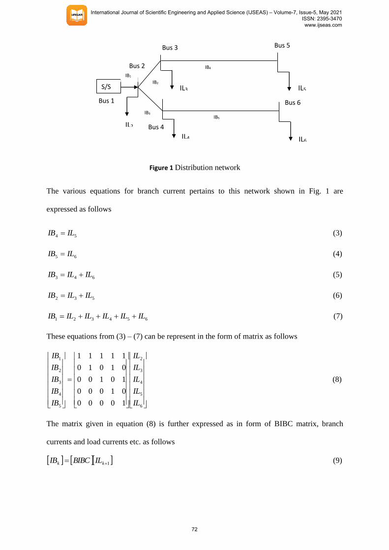
Figure 1 Distribution network

The various equations for branch current pertains to this network shown in Fig. 1 are

expressed as follows

54 ILIB = (3)

65 ILIB = (4)

643 ILILIB += (5)

532 ILILIB += (6)

654321 ILILILILILIB ++++= (7)

These equations from (3) – (7) can be represent in the form of matrix as follows

=

6

5

4

3

2

5

4

3

2

1

10000

01000

10100

01010

11111

IL

IL

IL

IL

IL

IB

IB

IB

IB

IB

(8)

The matrix given in equation (8) is further expressed as in form of BIBC matrix, branch

currents and load currents etc. as follows

1+= kk ILBIBCIB (9)

S/S

Bus 1

Bus 2

Bus 3

Bus 4

Bus 5

Bus 6

IB1

IB2

IB3

IB4

IB5

IL2

IL3

IL4

IL5

IL6


72

Where, BIBC is matrix given as 0 and 1 elements, [IB] and [IL] are also defined above

equations. Moreover, the branch current bus voltage (BCBV) is defined as follows. The

BCBV matrix is related to BIBC matrix which is given in above equations. These relationship

are obtained with the help of Kirchhoff’s voltage law (KVL) is applied in forward loop.

matrix impedancebranch is e, wher ZDZDBIBCBCBVT

= (10)

ZD is one of the matrix is called branch impedance matrix having diagonal elements are 1

remaining all elements are 0 (zero)

MODELING OF LOAD DEMAND:

In this present paper load demand is considered as real time load model as constant power

load (P), constant current load model (I), constant impedance load model (Z) and composite

load model (ZIP). These combined load models are basically characterized by per phase

complex power as line to neutral voltage. The complex power in the form of voltage is

expressed as

=+= SSjQPS or (11)

= VV (12)

Further, load current for constant power for both type i.e. (real and reactive) is defined as

( ) −

=

V

SIL pq (13)

In this expression shown in equation (13) the bus voltage magnitude is not remain constant at

time of iterations are executed in order to obtain convergence process.

Further, the next load demand profile i.e. constant impedance is expressed as


73

=S

VZ

2

Impedance (14)

Moreover, the load current is basically function of impedance is expressed as follows

( ) −=Z

VILZ (15)

LOAD PROFILE AS FUNCTION OF CURRENT:

This is the load profile is constant current load profile hence the value of current is change

according to following equation

( ) −

=

=

V

S

V

SILi

*

(16)

In equation (16) and are power factor angle and voltage angle respectively

ZIP TYPE OF LOAD MODEL:

It is the special category of load in which three quantities i.e. impedance (Z), current (I), and

power (P) are all remains constant during operation and their value taken in some proportion

to make the ZIP type load. In this load the total current which is entering in the load is sum of

all current components in order to obtain ZIP load profile. In this study the coefficient of

different load profile are taken as follows

COEFFICIENT OF ZIP:

The description of ZIP load model is given as follows

a) Z type load profile is considered as ZP, in this study its value is taken as 0.3

b) I type load profile is considered as IP, in this study its value is taken as 0.1

c) PQ type load profile is considered as SP, in this study its value is taken as 0.6


74

As the sum of all considered parameters is 1. Therefore, ZP+IP+SP = 1, further, load current

is represent as follows

pqizZIP IIIIL ++= and pqpqiizz ILSPIILIPIILZPI === and , (17)

LOAD FLOW ALGORITHM FOR DISTRIBUTION SYSTEM:

In this section algorithm adopted for evaluation of solution of load is discussed. There are

several steps which are using are given as follows

• Step 1: Data of branch and load data are read

• Step 2: Calculate the branch current and injected current from bus using the different

equations

• Step 3: Determine BIBC matrix

• Step 4: Determine the three matrices these are [BIBC] and [BCBV] and impedance

matrix is [ZD]

• Step 5: Calculate [DLF] matrix by [DLF] = [BCBV]*[BIBC]

• Step 6: Estimate [IB] = [BIBC]*[IL] and [ V] = [DLF]*[IL]

• Step 7: Fix iteration counter K = 0

• Step 8: Update iteration counter K = K + 1

• Step 9: Determine voltage at each bus for different load models

KK ILDLFV = +1

• Step 10: Calculate updated voltage 101 ++ += KK VVV

• Step 11: check tolerance level is obtained i.e. ( ) ( ) tolerance1 −+ KVKV , go to

step 8

• Step 12: Estimate current of each branch and hence calculate system power loss

• Step 13: Estimate bus voltage magnitude and print the results

• Step 14: End


75

DESCRIPTION OF OBTAINED RESULTS:

In this research article load flow of solution is applied on 85-bus network. The single line

representation of considered 85-bus network is shown in Fig. 2. Moreover, it is evident from

Fig. 3 that the voltage profile at various for different load demand. From this figure it is

observed that voltage at various buses is lowest in values for const power load while the

voltage values are higher for constant impedance load demand and for constant current load

model the voltage values are in between in constant power and constant impedance.

Furthermore, Fig. 4 is representing the branch current profile for different load model. From

this figure it is noticed that branch number 1 to 9 current required by different load model is

different additionally, up to branch 1 to 9 the constant power load profile require more current

as compare to other load profile such as constant impedance and constant current load model.

Secondly, constant impedance load model required minimum value of current for branch

number 1 to 9 and for constant current load model required less current as compare to

constant power load model and more current required from constant impedance load model.


76

1

2

3

4

5

6

7

8

9

10

11

12

13

14

15

16

17

18

19

20

21

22

23

24

46

47

45

44

57

58

5960

61

62

65

66

64

63

77

70

69

68

71

67

73

74

72

76 75

25

26

27

28

29

30

31

32

33

34

35

36

40

41

4243

38 37

39

48

49

50

51 56

54

53

52

55

79

78

80

81

82

83

84

85

Sub-station

Figure 2: Representation of 85-bus network


77

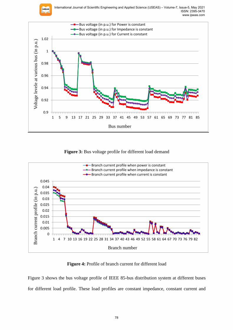
Figure 3: Bus voltage profile for different load demand

Figure 4: Profile of branch current for different load

Figure 3 shows the bus voltage profile of IEEE 85-bus distribution system at different buses

for different load profile. These load profiles are constant impedance, constant current and

0.9

0.92

0.94

0.96

0.98

1

1.02

1 5 9 13 17 21 25 29 33 37 41 45 49 53 57 61 65 69 73 77 81 85

Volt

age

level

e at

var

iou

s b

us

(in p

.u.)

Bus number

Bus voltage (in p.u.) for Power is constantBus voltage (in p.u.) for Impedance is constantBus voltage (in p.u.) for Current is constant

0

0.005

0.01

0.015

0.02

0.025

0.03

0.035

0.04

0.045

1 4 7 10 13 16 19 22 25 28 31 34 37 40 43 46 49 52 55 58 61 64 67 70 73 76 79 82

Bra

nch

curr

ent

pro

file

(in

p.u

.)

Branch number

Branch current profile when power is constantBranch current profile when impedance is constantBranch current profile when current is constant


78

constant power load demand. From this figure it is observed constant impedance load has

maximum value of bus voltage and constant power load has lowest value of bus voltage at

different buses and constant current load profile has medium value of bus voltage between

constant impedance and constant power load profile. Figure 4 shows the current profile of

different branches for different load profile as it is observed from this figure that constant

power load has higher value of branch current profile while constant impedance has lower

value of branch current profile.

CONCLUSIONS:

The present research article elaborate the load flow solutions of different load demand models

these load models are constant impedance load demand, constant current load demand and

constant power load models. The load flow solutions are performed by BFS based method in

this method in this method BIBC and BCBV matrices are formed in order to obtained

solutions of load flow in form of branch current, bus voltage and hence obtained the power

flow in each branch which helps to estimate the system power losses for further helpful to

restructure, reinforcement and expansion of existing distribution network. The program for

solution of load flow equations is formed in MATLAB environment and obtained results it is

found that voltage value in p.u. at various buses for various load model from this it is noticed

that pattern of voltage is almost similar but constant power load model has lower value of

voltage and this value is higher for constant current load model and constant impedance load

model. Further, the branch profile for all considered load model is almost similar. These

results are obtained by considering 85-bus network for validate the algorithm.

REFERENCES

[1] R. E. Brown, electric power distribution reliability, CRC press, 2008.


79

[2] Keane et al., “State-of the –Art Techniques and Challenges Ahead for Distributed

Generation Planning and Optimization,” IEEE Transactions on Power Systems, 28 (2),

1493-1502, 2013

[3] Pecas Lopes, N. Hatziargyriou, J. Mutale, P. Djapic, N. Jenkins. “Integrating

distributed generation into electric power systems: a review of drivers, challenges and

opportunities,” Electric Power Systems Research, 77, 1189-1203, 2007.

[4] P. S. Georgilakis and N. D. Hatziargyriou. “Optimal distributed generation placement

in power distribution networks: models, methods, and future research,” IEEE

Transactions on Power System, 3, 3420-3428

[5] T. Ackermann, G. Andersson, and L. Soder. “Distributed generation: a definition,

Electric Power Systems Research, 57, 195-204, 2001

[6] Y. A. Katsigiannis and P. S. Georgilakis. “Effect of customer worth of interrupted

supply on the optimal design of small isolated power systems with increased

renewable energy penetration,” IET Generation Transmission Distribution, 7 (3), 265-

275, 2013

[7] Mohd Zamri Che Wanik, Istvan Erlich, and Azah Mohmed. “Intelligent Management

of Distributed Generators Reactive Power for Loss Minimization and Voltage

Control,” MELECON-2010, IEEE Mediterrnean Electro-technical Conference, 2010

[8] N. C. Sahoo, S. Ganguly, D. Das. “Recent advances on power distribution system

planning: a state-of-the-art survey,” Energy Systems. 4, 165–193

[9] D. Q. Hung, N. Mithulananthan, R.C. Bansal. “Analytical expressions for DG

allocation in primary distribution networks,” IEEE Transactions on Energy

Conversion, 25 (3), 814-820

[10] D. Das. “Reactive power compensation for radial distribution networks using genetic

algorithm,” International Journal of Electrical Power & Energy Systems, 24 (7), 573-

581, 2002


80

[11] A.M. El-Zonkoly. “Optimal placement of multi-distributed generation units including

different load models using particle swarm optimization,” IET Generation

Transmission Distribution, 5 (7), 760-771, 2011

[12] S.H. Horowitz, A.G. Phadke. Power System Relaying, 2nd Ed. Baldock: Research

Studies Press Ltd, 2003

[13] S. Ghosh and D. Das. “Method for load-flow solution of radial distribution networks,”

IEEE Proceedings on Generation, Transmission & Distribution, 146 (6), 641- 648,

1999

[14] J. H. Teng. “A Direct Approach for Distribution System Load Flow Solutions,” IEEE

Transaction on Power Delivery, 18 (3), 882-887

[15] Sahib Khan and Arsan Ali. “CLIFD: A novel image forgery detection technique using

digital signatures” Journal of Engineering Research, 9 (1), 168-175, 2021.

[16] Abdelmoula Rihab, Ben Hadj Naourez, Chaieb Mohamed and Neji Rafik. “Multi-

objective optimization of a series hybrid electric vehicle using DIRECT algorithm”

Journal of Engineering Research, 9 (1), 151-167, 2021

[17] Mishal Al-Gharabally, Ali F Almutairi and Ayed A. Salman. “Particle swarm

optimization application for multiple attribute decision making in vertical handover in

heterogenous wireless networks” Journal of Engineering Research, 9 (1), 176-187,

2021


81

Documents

Load flow solutions of radial distribution system using