LIQUID FILM FORMATION BY SPRAY & DROPLET

IMPACT ON A SOLID SURFACE

By

Alireza Dalili

A thesis submitted in conformity with the requirements

for the degree of Doctor of Philosophy

Graduate Department of Mechanical and Industrial Engineering

University of Toronto

© Copyright by Alireza Dalili 2016

ii

ABSTRACT

Liquid Film Formation by Spray & Droplet Impact on a Solid Surface

Alireza Dalili

Doctor of Philosophy

Graduate Department of Mechanical and Industrial Engineering

University of Toronto

2016

Formation of liquid films through the deposition of droplets and spray onto a solid surface

was studied experimentally. Experiments were done to observe the coalescence of highly viscous

liquid droplets (87 wt% glycerin-in-water solutions) deposited onto a flat, solid steel plate.

Droplets were deposited sequentially in straight lines or square droplet arrays. Droplet center-to-

center distance was varied and the final dimensions of lines and sheets measured from

photographs. When overlapping droplets were deposited surface tension forces pulled impacting

droplets towards those already on the surface, a phenomena known as drawback. At large

overlaps droplets deposited in a line or square array coalesced to form a circular film. When the

droplet center-to-center distance increased, leading to less interaction, long, thin lines and square

sheets were formed. As overlap was further decreased lines and sheets became discontinuous. A

simple model was developed to predict the conditions under which rupture occurred. The lowest

droplet overlap ratio (defined as droplet overlap distance divided by droplet spread diameter) at

which a continuous liquid film could be formed was λ = 0.293. Further studies with a pneumatic

droplet generator that put down multiple droplets simultaneously confirmed this finding. In

addition, spray experiments also exhibited the drawback effect during droplet coalescence and

showcased the need to spray small droplets with large overlap in order to form a uniform thin

film. Bubble entrapment and escape from sprayed paint films of different thickness was analyzed

iii

and the number, diameter and velocity of air bubbles were determined. Bubbles were observed to

escape from both upward and downwards facing surfaces. Concentration gradients due to solvent

evaporation in a paint film create surface tension variations that drive Marangoni flows, which

bring bubbles to the paint surface. An analytical one-dimensional model of solvent diffusion was

used to calculate solvent concentration variations in the paint film and the Marangoni number.

iv

ACKNOWLEDGMENTS

I would like to express my deepest gratitude and appreciation to my supervisor, Professor

Sanjeev Chandra, for his invaluable guidance and consistent encouragement throughout my PhD

study. Without his help this dissertation would not have been possible. It has been an honour to

conduct research under his supervision.

I would also like to thank Professor Javad Mostaghimi who offered me valuable advice and

shared his expertise and research insights during my program.

My sincere thanks are extended to my thesis committee member, Professor Markus

Bussmann from the Department of Mechanical and Industrial Engineering at University of

Toronto.

I am also grateful to Professor Nasser Ashgriz from the Department of Mechanical and

Industrial Engineering at University of Toronto and Professor Alidad Amirfazli from the

Department of Mechanical Engineering at York University for participating in my SGS Final

Oral Exam.

Special gratitude goes to Dr. H.T. Charles Fan, Dr. H.H. (Harry) Kuo and Mr. Joseph C.

Simmer from General Motors R&D and funding sources, Natural Sciences and Engineering

Research Council of Canada (NSERC) and General Motors Canada.

Finally, I dedicate this thesis along with my heartfelt gratitude and love to my wife, Maryam,

and to my parents and family.

v

TABLE OF CONTENTS

ABSTRACT ................................................................................................................................... ii

ACKNOWLEDGMENTS ........................................................................................................... iv

TABLE OF CONTENTS ............................................................................................................. v

LIST OF FIGURES .................................................................................................................... vii

LIST OF TABLES ...................................................................................................................... xii

NOMENCLATURE ................................................................................................................... xiii

CHAPTER 1

INTRODUCTION ..................................................................................................................... 1

1.1 Automotive Paint Application ...................................................................................... 1

1.2 Droplet Coalescence ..................................................................................................... 4

1.3 Bubble Entrapment ....................................................................................................... 6

1.4 Thesis Objectives .......................................................................................................... 9

1.5 Thesis Organization .................................................................................................... 10

CHAPTER 2

FORMATION OF LIQUID SHEETS BY DEPOSITION OF DROPLETS ON A

SURFACE ................................................................................................................................ 11

2.1 Introduction ................................................................................................................ 11

2.2 Experimental System .................................................................................................. 12

2.3 Results & Discussion .................................................................................................. 15

2.4 Conclusion .................................................................................................................. 34

CHAPTER 3

FORMATION OF LIQUID SHEETS BY DEPOSITION OF MONO-DISPERSE

SPRAYS ON A FLAT SURFACE.......................................................................................... 36

3.1 Introduction ................................................................................................................ 36

3.2 Experimental System .................................................................................................. 37

3.3 Results & Discussion .................................................................................................. 39

3.4 Conclusion .................................................................................................................. 51

vi

CHAPTER 4

FORMATION OF LIQUID SHEETS BY SPRAYING ON A SURFACE ........................ 53

4.1 Introduction ................................................................................................................ 53

4.2 Experimental System .................................................................................................. 53

4.3 Results & Discussion .................................................................................................. 57

4.4 Conclusion .................................................................................................................. 64

CHAPTER 5

BUBBLE ENTRAPMENT AND ESCAPE FROM SPRAYED PAINT FILMS ............... 65

5.1 Introduction ................................................................................................................ 65

5.2 Experimental System .................................................................................................. 66

5.3 Results & Discussion .................................................................................................. 70

5.4 Conclusion .................................................................................................................. 91

CHAPTER 6

SUMMARY, CONCLUSIONS AND FUTURE WORK ..................................................... 93

6.1 Summary & Conclusions ............................................................................................ 93

6.2 Contributions .............................................................................................................. 96

6.3 Future Work ................................................................................................................ 96

REFERENCES ............................................................................................................................ 97

APPENDIX A

ENGINEERING DRAWING OF MECHANICAL PARTS ............................................. 106

APPENDIX B

TRANSLATION MOTION SYSTEM AND COMPUTER SOFTWARE ...................... 112

APPENDIX C

PHASE DOPPLER PARTICLE ANALYZER (PDPA) .................................................... 116

vii

LIST OF FIGURES

Figure 1.1: Various paint defects: (a) orange peel (b) running and sagging (c) wrinkling (d)

bubble entrapment [10, 11] ............................................................................................................. 3

Figure 2.1: Schematic and picture of the experimental system .....................................................14

Figure 2.2: Schematic showing deposition of droplets to form a line. Equilibrium spread

diameter of a single droplet after it impacted on the substrate, Ds, droplet center-to center

distance, L, stage speed, u ..............................................................................................................15

Figure 2.3: Lines formed by twelve 87 wt% glycerin droplets deposited on a steel substrate with

varying center-to-center spacing (L) ............................................................................................. 16

Figure 2.4: 1-D Drawback Index (𝜃1𝐷) as a function of overlap ratio (𝜆) for 87 wt% glycerin

lines. The curve shows the critical drawback index below which lines are no longer

continuous…. .................................................................................................................................19

Figure 2.5: Photograph of incremental build-up of 87 wt% glycerin liquid sheets produced at

λ = 0.88 and λ = 0.37. The final frame is taken 30 minutes after deposition, showing that the film

shape is stable ................................................................................................................................20

Figure 2.6: Photographs of 87 wt% glycerin liquid sheet produced at various overlap ratios (λ).

The red square indicates the ideal liquid sheet that should completely wet the surface with square

side length of Dy = Ds+(m-1)L where Ds = 5.86 mm, m = 12 droplets and L varies with overlap

ratio ................................................................................................................................................21

viii

Figure 2.7: a. Enlarged view of the film with λ = 0.25 film with angle α defined. b. Droplet

interaction in the λ = 0.25 film. The movement of the edge of the first droplet in each row due to

contact with the other droplets is indicated by the red arrows (∆x) .............................................. 23

Figure 2.8: 2-D Drawback Index (θ2D) variation with overlap ratio (λ) for 87 wt% glycerin liquid

sheets. The solid symbols show the sheets that remained intact and the hollow symbols sheets

that ruptured. All sheets that ruptured had θ2D < 1 and λ < 0.293..................................................25

Figure 2.9: a. Interaction between droplets in a 2-D liquid film generated from a stationary

nozzle and landing on a moving substrate. b. The droplet overlap ∆C is found by calculating the

diagonal length (OT) of the third and fifth droplets and subtracting the distance (OQ) to the

seventh droplet ...............................................................................................................................28

Figure 2.10: Measured circularity of the 2-D liquid films as a function of overlap ratio. The

horizontal lines mark the circularity of a perfect circle and a square ............................................30

Figure 2.11: Dimensionless film thickness (t/D) variation with overlap ratio (λ) ........................ 31

Figure 2.12: Dimensionless film thickness (t/D) variation with impact Reynolds number for

various Weber number values ........................................................................................................34

Figure 3.1: Schematic and picture of the experimental system .....................................................38

Figure 3.2: Photos of 10 second 87 wt% glycerin mono-disperse spray hitting the Plexiglass

substrate .........................................................................................................................................40

Figure 3.3: Evidence of drawback during droplet deposition ........................................................41

ix

Figure 3.4: Fraction of observable area covered by fluid over 20 second recording time ............42

Figure 3.5: Variation of Droplet Center-to-Center Distance (L) with time ...................................47

Figure 3.6: Variation of Overlap Ratio (λ) with time ....................................................................47

Figure 3.7: Representative arrangement of maximum number of non- overlapping circles that can

be packed into a square area of 2268 mm2 with Ds = 3.25 mm [50] .............................................49

Figure 3.8: Predicted average area coverage calculated for experimental conditions presented in

this chapter, namely m = 458 droplets and Ds = 3.25 mm .............................................................51

Figure 4.1: Schematic of the 87 wt% glycerin spray experimental setup ......................................55

Figure 4.2: Picture of spray fixture. Fixture has adjustable brackets at the four corners ..............57

Figure 4.3: Accumulation of spray droplets on the substrate ........................................................58

Figure 4.4: The time evolution of areas during and after spraying ................................................59

Figure 4.5: Coalescence and drawback in spray droplets ..............................................................60

Figure 4.6: Coalescence and drawback in spray droplets after the spray is shut off .....................61

Figure 4.7: A side view of equilibrium spreading diameter of each droplet (𝐷𝑠1 , 𝐷𝑠2), spreading

diameter, 𝐷𝑥, droplet center-to center distance, 𝐿, contact angle, 𝜃.…………. ............................62

x

Figure 5.1: Change in (a) viscosity and (b) surface tension of model paint with variation of

solvent concentration. The data for these graphs were provided by Javaheri [52]. .......................67

Figure 5.2: Picture of the experimental system .............................................................................70

Figure 5.3: Bubbles in 260 μm thick paint film .............................................................................71

Figure 5.4: Change in bubble density with time for paint films of varying thickness ...................72

Figure 5.5: Change in Sauter Mean Diameter (SMD) of bubbles with time for paint films of

varying thickness ...........................................................................................................................74

Figure 5.6: Change in film and bubble velocity over time for paint films of varying

thickness……. ................................................................................................................................75

Figure 5.7: Bubbles resting at the phase interface (model paint-air) before escaping ...................77

Figure 5.8: Thin liquid film between the bubble and the interface ................................................78

Figure 5.9: Bubbles in 150 μm thick upward and downward facing paint films ...........................79

Figure 5.10: Change in Sauter Mean Diameter (SMD) of bubbles with time for 150 μm thick

upward and downward facing paint films ......................................................................................80

Figure 5.11: Bubble escape mechanism.........................................................................................81

Figure 5.12: Bubble density for 87 wt% glycerin film ..................................................................82

Figure 5.13: Schematic of modeling parameters for drying of paint film at room

temperature……. ...........................................................................................................................84

xi

Figure 5.14: Weight loss as a function of time for paint films of varying thickness .....................86

Figure 5.15: Reduced desorption curves for paint films of varying thickness ..............................87

Figure 5.16: Solvent concentration profiles as a function of time for: (a) 100 μm and (b) 450 μm

thick paint films .............................................................................................................................89

Figure 5.17: Marangoni number as a function of time for paint films of varying thickness .........90

Figure A.1: Opal diffusing glass holder .......................................................................................107

Figure A.2: Mono-disperse spray nozzle body ............................................................................108

Figure A.3: Mono-disperse spray nozzle plate ............................................................................109

Figure A.4: Spray fixture substrate holder ...................................................................................110

Figure A.5: PDPA spray mounting plate .....................................................................................111

Figure B.1: Software interface developed for motion stage control and droplet deposition

[16]…… ...................................................................................................................................... 113

Figure C.1: TSI PDPA system used for measuring spray droplet size ........................................116

Figure C.2: TSI FlowSizer software Interface [66] .....................................................................117

xii

LIST OF TABLES

Table 2.1: Properties of 87 wt% glycerin in water solution and other fluids commonly used in

painting and printing applications. The properties of 87 wt% glycerin in water solution and paint

were measured at 25 °C. The properties of the paraffin wax and printer ink were measured at

their respective melting temperatures of 70 °C and 95 °C ............................................................12

xiii

NOMENCLATURE

Variable Unit

A Area of liquid sheet m2

𝐴𝑊 Wetted surface area m2

𝐴𝐼𝑊 Ideal wetted surface area m2

C Concentration -

Ci Initial volatile concentration -

C∞ Volatile concentration in atmosphere -

∆C Concentration difference across the paint film -

D Diameter m

𝐷𝑠 Droplet spread diameter m

𝐷𝑦 Droplet line length m

Dv Volatile diffusivity in paint m2/s

d10 Mean Diameter m

d32 Sauter Mean Diameter m

𝐹𝜎 Surface tension force N/m

𝐹𝜇 Viscous shear force N/m

g Gravitational acceleration m/s2

h Liquid film thickness (height) m

J Volatile mass flux kg/m2s

L Droplet center-to-center distance m

L Paint film thickness m

M Mass kg

𝑚 Number of deposited droplets -

n Row (Line) in a liquid sheet array -

P Perimeter of liquid sheet m

𝑝 Pressure N/m2

r Droplet radius m

r Bubble radius m

t Time s

t Liquid film thickness m

U Droplet impact velocity m/s

U Bubble velocity m/s

xiv

V Liquid volume m3

x Length of liquid sheet m

x Vertical coordinate m

y Height of liquid sheet m

Greek Letters

α Coefficient in mass transfer equation at paint surface kg/m2s

βa Advancing contact angle °

𝜃 Static contact angle °

𝜅 Surface curvature 1/m

𝜌 Liquid density kg/m3

𝜌𝑣 Volatile partial density kg/m3

𝜌𝑝 Bubble density kg/m3

𝛥𝜌 Difference between model paint and bubble density kg/m3

µ Dynamic viscosity N.s/m2

σ Surface tension N/m

λn Eigenvalues -

𝜆 Overlap ratio -

𝜃1𝐷/2𝐷 1-Dimension / 2-Dimension drawback index -

ξ Droplet spread factor -

Dimensionless Numbers

We Weber number -

Re Reynolds number -

Bi Biot number -

Fo Fourier number -

𝑀𝑎 Marangoni number -

1

CHAPTER 1

INTRODUCTION

1.1 AUTOMOTIVE PAINT APPLICATION

An automobile’s colour and appearance creates the consumers’ first impression about a car

and often serves as one of the key factors in making a purchasing decision. However, automobile

paint and surface finish also acts as a corrosion and abrasion resistant coating that protects the

vehicle over a service life of many years. Therefore, the painting of cars is a very complex and

important step in production subject to very strict quality control. The paint shop can constitute

anywhere from 30-50% of the total cost of a typical assembly plant [1]. Over 80% of all

environmental concerns in automobile assembly are attributed to painting and related processes

[2]. For instance, these processes act as the largest source of regulated chemicals including

volatile organic compounds and other air pollutants [2]. As a result, car manufacturers shoulder a

significant cost burden to capture these emissions and dispose the waste material.

Currently paints are applied to the body in multiple layers with the use of electrostatic

rotating bell (ESRB) atomizers, where paint is directed onto the inner bell surface that is

maintained at a voltage of 50-90 kV and rotates at around 50,000 rpm, to break up the paint and

expel it through centrifugal forces [3, 4, 5, 6]. High velocity shaping air and often a charged

pattern control ring is used to force the charged particles towards the surface. Robot

manipulators are used to position the paint atomizers.

2

As described by [5, 7], paint curing of automotive car bodies is a complex and energy

consuming task. Paint is usually cured in 3 steps: flash-off, convection and radiation as

mentioned by [5]. As described by [6], in the flash-off step, solvents evaporate from the wet film

and the paint film flows and smoothes out. The ambient temperature needs to be kept constant

and sufficient time must be afforded for flash-off. For instance, GM uses an ambient flash-off

period of 2 minutes [5]. After flash-off, convection curing is carried out by circulating heated air

around the part in an oven [6, 8, 9]. To reduce the curing period, radiation is used as well. As an

example, GM first carries out 5 minutes of radiation curing before subjecting the part to a 20

minute forced convection curing [5]. The entire process is carried out at 121 oC [5].

BASF and HMG Paints, [10, 11], have a list of paint defects along with the definition,

causes, prevention and repair measures for each one. Figure 1.1 illustrates a sample of these poor

paint finishes. For instance, a paint film that is not flat exhibits an “orange peel” finish

(Fig. 1.1a). The non-uniform paint layer can be caused by larger than desired droplets in the

spray, low droplet impact velocity or high paint viscosity. High paint viscosity means that paint

droplets do not have enough time to spread, coalesce and level out in order to form a flat paint

surface. Paint sagging (Fig. 1.1b) is caused by gravitational forces inducing flow of paint layers

on inclined surfaces [12]. Reducing paint viscosity leads to improved leveling of the paint film

and lessens the orange peel effect, but worsens paint sagging. Also, if the applied paint film is

thicker than usual, it will lead to sagging (running) of the paint, while a thin paint film can lead

to orange peel [13]. In addition, as the paint dries and the volatile components evaporate, the

composition of the paint layer varies with depth. The viscosity, density and surface tension of

paint near the free surface becomes greater than lower layers [14]. This leads to convection

driven flows in the paint film and wrinkling of the paint surface (Fig. 1.1c). Moreover, bubbles

3

can be entrapped in the paint during impact of the spray droplets or can be generated by

evaporation of gases during curing (Fig. 1.1d).

(a) (b) (c) (d)

Figure 1.1: Various paint defects: (a) orange peel (b) running and sagging (c) wrinkling (d)

bubble entrapment [10, 11]

The quality of sprayed paint layers depend on a large number of parameters such as droplet

size, impact velocity, spray angle and paint properties (viscosity, density, surface tension). At the

present time, the optimal spray parameters are found through trial-and-error, a time-consuming

and expensive process.

The aim of this thesis was to further understand the causes of paint defects and establish

concrete relationships between the paint application parameters and the eventual quality of the

painted surface.

4

1.2 DROPLET COALESCENCE

In painting and coating applications droplets are sprayed on a solid surface to form a smooth,

continuous liquid film. It is often desirable to make the film as thin as possible, but surface

tension may prevent droplets deposited on a solid surface from wetting the surface properly and

flattening into a thin layer. Interactions between droplets and their subsequent movement can

also make the surface of the liquid layer uneven. As the film dries and hardens these surface

undulations become visible as defects in the coating.

In addition to automotive coatings, there are other applications where droplet interactions

have a significant impact on the quality of the finished product. An ink-jet printer creates text or

images on paper by placing small ink droplets in a pattern. This well-established technology is

increasingly being applied in newly emerging fabrication methods that use droplet-on-demand

generators coupled with computer-controlled motion stages to deposit polymers to fabricate

electronic circuits [15], build three-dimensional components out of wax, metal or ceramic [16],

or even create organs by depositing living tissue on soft scaffold structures [17]. In all of these

applications it is important that droplets remain where they are placed so that their desired

configuration is maintained. However, capillary forces between touching droplets can displace

them from their original position, an effect known as “drawback”, reducing the resolution with

which components can be made. Drawback reduces the resolution of ink-jet printed images,

diminishes the dimensional tolerance of objects created by 3D printing and can cause

displacement of solder bumps placed on printed circuit boards.

Numerous experimental and analytical studies have been carried out to investigate the

coalescence of droplets [18-27]. Duineveld [18] studied the stability of ink-jet printed line of

5

liquid with zero receding contact angle on a flat uniform surface both experimentally and

theoretically. The lines became unstable if the liquid-substrate contact angle became larger than

the advancing contact angle. In [19], the authors considered the coalescence of two water sessile

drops during condensation and studied its kinetics both experimentally and theoretically. They

found the relaxation time to be extremely large which was attributed to the strong dissipation that

occurs during the motion of the contact line. Roisman et al. [20] focused on the impact of two

drops on a solid dry surface. Parameters such as droplet diameter, impact velocity, time interval

between the drops and their distance were controlled. The shape of the liquid film on the surface,

the interface between the two drops and the shape of the uprising sheets was observed.

Analytical models were proposed for single drop impact that took into account surface tension,

wettability, viscous drag and inertia as well as inertia dominated symmetric impact of two

identical drops. Authors of [21] studied the coalescence of a pendent and a sessile drop for

different viscosity and drop sizes. The droplets coalesced rapidly due to large curvature and

unbalanced surface tension force in the neck region. Increasing liquid viscosity led to sharper

neck curvature. Ri Li et al. [22] examined drawback during the deposition of overlapping molten

wax droplets while varying substrate temperature, droplet overlap ratio and the time between

impacts of droplets. In a subsequent paper [24] they studied the coalescence of a falling droplet

with a stationary sessile droplet, using high-speed video to record coalescence dynamics, shape

evolution and contact line movement. Narhe et al. [23] considered the coalescence of water

droplets growing in a condensation chamber as well as through syringe deposition. The authors

saw that the initial kinetic energy given to the droplet greatly affected the coalescence dynamics

such that syringe deposition induced large oscillations while condensation coalescence did not

exhibit such oscillations and as a result the relaxation time was 10-100 times slower. Gao and

6

Sonin [25] investigated the conditions required for precise deposition of molten microdrops

under controlled thermal conditions. Columnar, sweep deposition on flat surfaces and repeated

sweep deposition for building larger objects were investigated. Castrejon-Pita et al. [26]

investigated the dynamics of impact and coalescence of glycerol/water droplets on a solid

surface by high-speed particle image velocimetry. Graham et al. [27] considered the coalescence

of a falling droplet with a sessile one on solid surface of various wettabilities through

experimental and numerical analysis. The droplet diameter, impact velocity and distance

between the impacting droplets were controlled. All of these studies were done using two or

more droplets deposited in a line. There has been no work done to examine interactions between

droplets deposited in two-dimensional sheets on a surface.

1.3 BUBBLE ENTRAPMENT

When liquid is atomized and sprayed on a surface, as in industrial paint processes, a large

number of bubbles are formed in the deposited layer [28]. This is a well-known problem in the

automotive paint industry and “defoaming agents”, which are typically surfactants, are added to

paints to minimize bubble entrapment [29]. Bubbles can create serious defects in car body

finishes. After paint is sprayed on automotive components they are baked in an oven to evaporate

the solvent and cure the paint. Evaporating solvent diffuses into any bubbles still in the paint,

expanding them until they burst through the paint surface and create visible pinholes [30].

A number of studies have been carried out to investigate the formation of air bubbles during

droplet impact [31-42]. Chandra and Avedisian [31] photographed the impact of a n-heptane

7

droplet onto a stainless steel surface at room temperature and observed the presence of a single

bubble at the point of impact. Mehdi-Nejad et al. [32] numerically simulated the droplet impact

for water, n-heptane and molten nickel droplets to investigate the effect of viscosity, velocity and

contact angle on bubble entrapment. They explained that the bubble forms due to the air gap

between the impacting droplet and the surface. As the droplet approaches the surface, the air in

the gap is forced out. Increased air pressure under the droplet leads to the creation of a

depression in its surface in which air is trapped. The maximum air pressure was seen to be

located directly below the center of the droplet where the bubble forms. Researchers in [33] used

ultrafast x-ray phase contrast imaging to visualize the evolution process of the air film into a

bubble. Investigators in [34, 35] saw bubble entrapment both at the center as well as underneath

the levitated spreading lamella.

Van Dam and Le Clerc [36] experimentally studied micro-sized water droplet impact and

observed bubble entrapment in almost all cases. They optically measured the droplet shape and

oscillation behavior during impact and proposed a model for the bubble volume based on impact

speed. Thoroddsen et al. [37] observed the evolution of the air disk under a droplet impacting

onto a solid surface as it contracted into a bubble under the center of the drop for a range of

Weber and Reynolds numbers. They measured the initial size and contraction speed of the air

disk. They found that the contraction speed of the bubble is independent of the wettability of the

liquid. Micro-bubble formation was often seen on the initial ring location. In addition, the

capillary wave propagation from the edge of the air disk to the center left a small droplet in the

middle of the bubble. Eggers [38] studied air entrainment through free-surface cusps. The author

proposed that the viscosity of the air drawn into the narrow channel of a cusp singularity is

8

enough to destroy the stationary solution and a sheet emanates from the cusp’s tip through which

air is entrained.

Elmore et al. [39] took high speed images of air-water interface dynamics of drop impact that

lead to reproducing bubbles and discussed the various phenomena seen during the process.

Thoroddsen et al. [40] studied bubble entrapment during droplet impact onto a liquid surface.

With the aid of an ultra-high-speed video camera, they studied the dynamics of the air sheet

under the center of the droplet as it contracts due to surface tension and forms a bubble. They

concluded that the contraction speed of the air sheet can be explained as a balance between

inertia and surface tension forces. They proposed a model for the initial bubble thickness and

radius based on the bottom curvature of the droplet and the Reynolds number. Deng et al. [41]

investigated bubble entrapment for droplet impact onto the surface of a deep pool of the same

liquid as the droplet. They found that viscosity has a weakening effect on capillary waves around

the crater which is responsible for the bubble pinching. They concluded that bubble size

decreases exponentially with increasing capillary number. Keij et al. [42] observed bubble

formation during the impact of a sessile droplet with a moving meniscus and concluded that the

size of the entrapped bubble depended very much on the initial location where the droplet and

the moving meniscus first made contact and coalesced. The process of bubble entrapment is

fairly well understood and various practices in industry attempt to minimize bubble entrapment

such as adding surfactant to the paint, altering the paint chemistry altogether or delaying the

placement of the painted surface in the oven for curing to allow for bubble escape, a practice

known as “flash-off”. However, it is not clear how bubbles escape from paint films and we

attempt to address it in this thesis.

9

1.4 THESIS OBJECTIVES

The goal of this thesis was to advance our understanding of droplet coalescence and bubble

entrapment during painting applications. Such knowledge would allow us to know the minimum

amount of material necessary to cover a certain area without having any ruptures in the liquid

film. The droplet size and overlap criteria required to create a uniform thin film could be

established. Furthermore, knowing the mechanism behind bubble escape, including the effect of

paint film thickness, bubble size and gravity could eventually lead to guidelines and

recommendations that enhance the quality of the painted surface. In order to achieve these

objectives the following was done:

Design and build an apparatus to create liquid films through deposition and coalescence of

individual droplets

Develop an analytical model to predict the shape, thickness and continuity of liquid films for

a given droplet size and spacing

Design and construct an experimental system to photograph the impact and amalgamation of

multiple droplets from a mono-disperse spray

Investigate the growth of liquid films generated from a mono-disperse spray and the effect of

droplet interactions on them

Design and build an apparatus to visualize liquid film formation by spraying on a surface

Study the evolution of liquid masses from a spray over time and determine the droplet size

and overlap criteria required to obtain a uniform thin film

Establish the mechanism by which bubbles escape from a paint film and estimate the

magnitude of the forces and flows involved in the process

10

1.5 THESIS ORGANIZATION

Chapter 2 describes the experimental and analytical work pertaining to the formation of

liquid films from depositing individual droplets. The liquid films obtained for different droplet

spacing are presented and a simple criteria is outlined on when continuous lines or sheets of

liquid should be expected for a given droplet size and spacing and what their shape and thickness

would be.

Chapter 3 focuses on visualization of liquid films formed by laying down multiple droplets

from a mono-disperse spray. Photographs of the liquid films are displayed and their growth

pattern and the effect of droplet interactions are explained.

Chapter 4 concentrates on the time evolution of liquid films formed from spray deposition

onto a surface and the droplet size and overlap criteria needed to attain a uniform thin film.

Chapter 5 presents the experimental and analytical work carried out on bubble entrapment

and escape from sprayed paint films of varying thickness. The process by which the bubbles

leave the film is articulated and an analytical model is used to calculate the magnitude of the

forces and flows responsible for bubble movement.

Chapter 6 outlines the main conclusions of this research work and provides recommendations

for future work in this area.

11

CHAPTER 2

FORMATION OF LIQUID SHEETS BY DEPOSITION OF

DROPLETS ON A SURFACE

2.1 INTRODUCTION

There are many applications in which it is vital for deposited droplets to remain in their

positions in order to maintain the desired pattern and arrangement. However, capillary forces

between neighbouring droplets can lead to their displacement from the initial position, an effect

known as “drawback”, reducing the quality of the final product. The study outlined in this

chapter was motivated by two questions. The first: how do droplet interactions influence the

shape of a liquid film printed on a solid surface? For example, if we deposit droplets in a square

array, will the perimeter of the sheet formed remain square? The second question: what is the

biggest surface area (corresponding to the thinnest liquid layer) we can cover with a given

volume of droplets before their spacing becomes so large that the liquid film ruptures due to

drawback?

This chapter reports the results of experimental investigation in which droplets of 87%

glycerin in water solutions, with viscosity two-orders of magnitude greater than that of pure

water, were deposited in lines and square arrays on a metal surface and their coalescence

photographed. The high viscosity of the liquid is typical of paints, polymers and waxes used in

coating applications. Table 2.1 lists the properties of the test liquid along with those of some

commonly used industrial fluids. The objective was to develop a simple criteria to predict when

12

continuous lines or sheets of liquid could be formed for a given droplet size and spacing and

what their shape and thickness would be.

density

(ρ) kg/m3

viscosity

(µ) cP

surface tension

(σ) mN/m

87 wt% glycerin

in water solution

[43, 44, 45]

1224 124 63.5

Paint [43] 1004.4 110 32.3

Paraffin wax [46] 771 5.4 22.4

Printer ink [47] 820 34.3 27.6

Table 2.1: Properties of 87 wt% glycerin in water solution and other fluids commonly used in

painting and printing applications. The properties of 87 wt% glycerin in water solution and paint

were measured at 25 °C. The properties of the paraffin wax and printer ink were measured at

their respective melting temperatures of 70 °C and 95 °C.

2.2 EXPERIMENTAL SYSTEM

Figure 2.1 gives a schematic diagram and picture of the experimental system used to form

droplets in a pattern on a substrate. An x-y motion stage (XYR-1010, Danaher Precision Motion,

USA) with 200 mm x 200 mm (8 in. x 8 in.) travel, controlled by software developed by Fang

[16], was used to position the substrate. The droplet generator system consisted of a stainless

steel tank filled with liquid and connected to a centrifugal pump (PA411-50MT, The Berns

Corporation, USA) that passes compressed liquid through stainless steel and plastic tubing to a

solenoid valve (8262H020, ASCO Valves, USA). A partially open needle valve (S-1RS6,

Swagelok, USA) was used to manually control the fluid flow upstream of the needle. That and a

pressure regulator (26A, Watts Water Technologies, USA) maintained a closed loop for fluid

flow and ensured no back flow into the pump. The solenoid valve was normally closed and could

be opened for a pre-determined period of time with a timer circuit that was triggered by a

13

computer and coordinated with the motion of the substrate. By varying the speed of the motion

stage, the center-to-center distance between droplets (L) was controlled. Droplets were deposited

at a constant frequency of 1 Hz. The exact position of the droplets varied due to variations in the

delay between triggering the solenoid valve and detachment of a droplet from the tip of the

needle. The uncertainty in positioning a droplet was ±0.14 mm.

Droplets of 87 wt% glycerin in water solution were made by opening the solenoid valve for

13 ms to allow liquid at 30 kPa pressure to pass through a 17 gage needle (7748-03, Hamilton

Company, USA) (with 1.47 mm outer diameter) and detach from the tip as a droplet. The

average droplet diameter (D) was measured to be 3.4 mm with a standard deviation of 0.01 mm;

all droplets had diameters within two standard deviations of the mean. The droplets impacted

with a velocity (U) of 1.1 m/s.

Still images of the final shape of droplets were captured at 2304x1728 pixel resolution using

a video camera (Sony HDR-CX100, Sony Corporation, USA). The spread diameter of a single

droplet (Ds) and the length (Dy) of a line formed by the coalescence of several droplets were

defined as shown in Figure 2.2 and measured using image analysis software (ImageJ, National

Institute of Health).

14

Figure 2.1: Schematic and picture of the experimental system

Pump Tank

Pressure

Regulator

Solenoid

Valve

Needle

Valve

Timer

DC Voltage Source

X-Y

Motion

Stage

15

Figure 2.2: Schematic showing deposition of droplets to form a line. Equilibrium spread

diameter of a single droplet after it impacted on the substrate, Ds, droplet center-to center

distance, L, stage speed, u.

2.3 RESULTS & DISCUSSION

The equilibrium spread diameter of a single droplet after it impacted on the substrate was

measured to be Ds = 5.86 mm and the equilibrium liquid-solid contact angle was 45°. The Weber

number (We= ρU2D/σ) for our experiments was calculated to be 80 and the Reynolds number

(Re= ρUD/μ) was 37. Since the contact angle was measured at the liquid/substrate interface, this

study only applies to hydrophilic surfaces in which the contact angle is less than 90°. Lines were

created by depositing twelve droplets onto the steel substrate with droplet center-to-center

distance, L, varying from 0.73 mm to 6.58 mm. The resulting lines are shown in Figure 2.3. As

evident in the images, as the overlap ratio decreases, the line becomes longer and thinner.

Decreasing the overlap ratio allows production of lines with more uniform thickness, but if the

overlap is too small the lines begin to break up.

16

0.73 mm (λ = 0.88)

1.45 mm (λ = 0.75)

2.17 mm (λ = 0.63)

2.96 mm (λ = 0.50)

3.68 mm (λ = 0.37)

4.41 mm (λ = 0.25)

5.13 mm (λ = 0.12)

5.86 mm (λ = 0.00)

6.04 mm (λ = -0.03)

6.58 mm (λ = -0.12)

Figure 2.3: Lines formed by twelve 87 wt% glycerin droplets deposited on a steel substrate with

varying center-to-center spacing (L).

80 mm

Direction of Droplet Landing

17

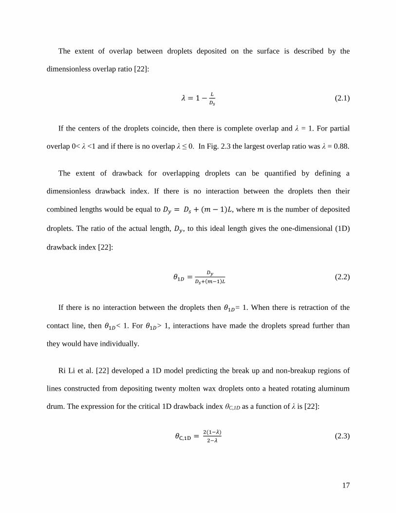
The extent of overlap between droplets deposited on the surface is described by the

dimensionless overlap ratio [22]:

𝜆 = 1 −𝐿

𝐷𝑠 (2.1)

If the centers of the droplets coincide, then there is complete overlap and λ = 1. For partial

overlap 0< λ <1 and if there is no overlap λ ≤ 0. In Fig. 2.3 the largest overlap ratio was λ = 0.88.

The extent of drawback for overlapping droplets can be quantified by defining a

dimensionless drawback index. If there is no interaction between the droplets then their

combined lengths would be equal to 𝐷𝑦 = 𝐷𝑠 + (𝑚 − 1)𝐿, where 𝑚 is the number of deposited

droplets. The ratio of the actual length, 𝐷𝑦, to this ideal length gives the one-dimensional (1D)

drawback index [22]:

𝜃1𝐷 =𝐷𝑦

𝐷𝑠+(𝑚−1)𝐿 (2.2)

If there is no interaction between the droplets then 𝜃1𝐷= 1. When there is retraction of the

contact line, then 𝜃1𝐷< 1. For 𝜃1𝐷> 1, interactions have made the droplets spread further than

they would have individually.

Ri Li et al. [22] developed a 1D model predicting the break up and non-breakup regions of

lines constructed from depositing twenty molten wax droplets onto a heated rotating aluminum

drum. The expression for the critical 1D drawback index θC,1D as a function of λ is [22]:

𝜃C,1D = 2(1−𝜆)

2−𝜆 (2.3)

18

The 1D model developed by Ri Li et al. [22] (Eq. 2.3) does not explicitly include surface or

liquid properties. However, the equilibrium spread diameter of a single droplet after impact on

the substrate (Ds) can either be measured from experiments or calculated from correlations that

are typically functions of We, Re, and liquid-solid contact angle. Ds determines both overlap ratio

(λ) and 1D drawback index (θ1D), making these variables and the models derived using them a

function of surface and liquid properties. Therefore, Eq. 2.3 can be used to predict the breakup

and non-breakup regions of the lines constructed in this study from depositing twelve 87 wt%

glycerin droplets onto a flat, solid steel plate at ambient temperature.

Figure 2.4 shows the 1D drawback index (𝜃1𝐷) variation with overlap ratio (𝜆) for twelve

drops, where each data point represents the average of five measurements. For 𝜃1𝐷< 1, drawback

has occurred. For large overlap (𝜆 ≥ 0.72), the drawback index became greater than 1 (𝜃1𝐷 >1),

meaning that interactions between droplets made them spread more than they would have if they

had landed on the bare substrate. The locus of Eq. 2.3 is also plotted in Figure 2.4. For a specific

λ, θ1D < θC,1D means the line will be broken, while θ1D > θC,1D means that the line will be

continuous. In the figure, solid symbols represent continuous lines and hollow symbols signify

broken lines. For the case of overlap ratio λ = 0.12, both continuous and discontinuous cases

were observed, depending on small variations in droplet placement, as it lands on the border

between the breakup and non-breakup regions. The theoretical model (Eq. 2.3) correctly predicts

the break up and non-breakup regions for the twelve 87 wt% glycerin droplet lines.

The incremental build-up of two-dimensional liquid sheets and the difference in the final

shape of the films for various overlaps were studied by creating 12x12 square droplet array with

varying overlap ratios. Figure 2.5 shows the process of creating sheets with overlaps of λ = 0.88

19

(L = 0.73 mm) and λ = 0.37 (L = 3.68 mm). The same droplet spacing was maintained in both x

and y directions for each sheet and the direction of droplet landing on the substrate is shown in

Figure 2.5. For large overlap (λ = 0.88) even a single line was in the form of a circle, while for

small overlap the droplets formed a continuous line. When 144 droplets were deposited in a

12x12 grid, they formed a circle at large overlap and a roughly square shape, narrower at the top

than the bottom, for small overlap. To ensure that the final shapes were stable, the sheets were

photographed again after 30 minutes. As can be seen in the last image in Figure 2.5, the shape

did not change significantly.

Figure 2.4: 1-D Drawback Index (𝜃1𝐷) as a function of overlap ratio (𝜆) for 87 wt% glycerin

lines. The curve shows the critical drawback index below which lines are no longer continuous.

0

0.2

0.4

0.6

0.8

1

1.2

1.4

0 0.2 0.4 0.6 0.8 1 1.2

θ1D

(1D

Dr

aw

ba

ck

In

de

x)

λ (Overlap Ratio)

Breakup

Non-breakup

Theoretical Prediction:

20

λ = 0.88 λ = 0.37

1 Line

2 Lines

4 Lines

6 Lines

8 Lines

10 Lines

12 Lines

12 Lines (30 min)

Figure 2.5: Photograph of incremental build-up of 87 wt% glycerin liquid sheets produced at

λ = 0.88 and λ = 0.37. The final frame is taken 30 minutes after deposition, showing that the film

shape is stable.

64 mm

21

A number of liquid films were made by depositing droplets in a square 12 x 12 array with

varying overlap ratios from λ = 0.88 to λ = –0.12. Figure 2.6 shows the final shapes obtained.

The squares marked on the images indicate the shape of the liquid sheet ideally desired, with side

length of Dy = Ds+(m-1)L, where in this case Ds = 5.86 mm, m = 12 droplets and L varies with

overlap ratio. By comparing the actual sheet to the square, one can clearly see the excess

spreading or drawback at different overlap ratios. At large overlap (λ≥0.75), the liquid sheets are

circular and significantly larger than the corresponding squares superimposed on them. They

become square at lower overlap 0.63≤λ≤0.37. Further decreasing the overlap (λ = 0.25) distorts

the film so that it is narrower at the top than the bottom. For λ≤0.25, the film begins to rupture as

drawback moves the droplets and creates holes in the film.

λ = 0.88 λ = 0.75 λ = 0.63

λ = 0.50 λ = 0.37 λ = 0.25

λ = 0.12 λ = 0.00 λ = -0.12

Figure 2.6: Photographs of 87 wt% glycerin liquid sheet produced at various overlap ratios (λ).

The red square indicates the ideal liquid sheet that should completely wet the surface with square

side length of Dy = Ds+(m-1)L where Ds = 5.86 mm, m = 12 droplets and L varies with overlap

ratio.

89 mm

22

Figure 2.7a shows an enlarged view of the film made with λ = 0.25, which has a distinctive

shape, narrowing towards the top. The angle α between the tangents to the two sides was

measured to be 70°. When droplets are deposited in overlapping lines, the first droplet in each

line contacts two previously deposited droplets, and is pulled by both of them as indicated by the

arrows in Figure 2.7b. The displacement of the droplets is visible in Figure 2.7a, producing the

scalloped edges of the film. Each successive line is therefore shorter than the previous. This

effect is additive as successive lines are deposited, so since the length of the first line is:

𝑥 = [(𝑚 − 1)𝐿 + 𝐷𝑠]𝜃1𝐷 (2.4)

The displacement of the first droplet in line n will be:

∆𝑥 = 𝑛[(𝑚 − 1)𝐿 + 𝐷𝑠](1 − 𝜃1𝐷) (2.5)

The vertical height of the sheet after n lines are placed is:

∆𝑦 = [(𝑛 − 1)𝐿 + 𝐷𝑠]𝜃1𝐷 (2.6)

The tangent of the angle α is therefore,

tan 𝛼 =∆𝑦

∆𝑥=

[(𝑛−1)𝐿+𝐷𝑠]𝜃1𝐷

𝑛[(𝑚−1)𝐿+𝐷𝑠](1−𝜃1𝐷) (2.7)

For the case of a square grid, where n = m

tan 𝛼 = 𝜃1𝐷

𝑛(1−𝜃1𝐷) (2.8)

Substituting the measured value of θ1D = 0.97 for λ = 0.25 and n = 12 we get α = 69.6° from Eq.

2.8, which is very close to the observed value of 70°.

23

𝑥 = [(𝑚 − 1)𝐿 + 𝐷𝑠]𝜃1𝐷

𝑥𝑖𝑑𝑒𝑎𝑙 = (𝑚 − 1)𝐿 + 𝐷𝑠

α

∆y

∆x

Row 3

a.

b. Row 2

Row 1

Row 12

2∆x

∆x

Row 4 4∆x

3∆x

Figure 2.7: a. Enlarged view of the film with λ = 0.25 film with angle α defined. b. Droplet

interaction in the λ = 0.25 film. The movement of the edge of the first droplet in each row due to

contact with the other droplets is indicated by the red arrows (∆x).

24

To quantify the extent of drawback in liquid sheets, the wetted surface area, AW, was

measured using image analysis software and normalized by the ideal area, AIW. The ideal wetted

area, marked by the square in each image of Figure 2.6, corresponds to the case where the

deposited droplets do not interact with one another so that the film is a square with side length

Ds+(m-1)L, where m is the number of droplets in one row of the array. The area of the square is

AIW = [Ds+(𝑚 −1)L]2. The ratio of AW to AIW gives a two-dimensional (2D) drawback index:

𝜃2𝐷 =𝐴𝑊

𝐴𝐼𝑊=

𝐴𝑊

[𝐷𝑠+(𝑚−1)𝐿]2 (2.9)

If we assume that both sides of the square sheet are pulled back by the same amount as a single

line of droplets, the actual wetted area may be approximated by:

AW = {[Ds+(𝑚 −1)L] θ1D} 2 (2.10)

Substituting Eq. 2.10 in Eq. 2.9 gives a relationship between the one-dimensional and two-

dimensional drawback indices:

θ2D = (θ1D)2 (2.11)

If there is no interaction between the droplets, 𝜃2𝐷 = 1. When there is retraction of the

contact line, then 𝜃2𝐷 < 1. For 𝜃2𝐷 > 1, interactions have made the droplets spread further than

they would have individually. 𝜃2𝐷 has been plotted as a function of overlap ratio (λ) for 2D

liquid sheets in Figure 2.8. At 𝜆 = 0.5, 𝜃2𝐷 ≈ 1, so that the shape of the film is very close to ideal

(see Figure 2.6). For an overlap of 𝜆 > 0.5, 𝜃2𝐷 >1, implying droplets landed on top of each

other and flowed outwards, spreading more than they would have if they had landed on the bare

substrate. Excess spreading is much more pronounced in the liquid sheet than it was in the case

25

of a single line (compare Figure 2.4 with Figure 2.8). Averaged over a large number of droplets,

the average overlap ratio remains the same for a given application.

The film will rupture if we attempt to spread the liquid over a larger area than it can cover,

i.e. if AIW > AW or alternately, if θ2D <1. The critical drawback index, below which the film will

be discontinuous, is θ2D,C = 1. Figure 2.8 shows that this criterion works well in practice: films

with θ2D <1 were seen to be ruptured.

Figure 2.8: 2-D Drawback Index (θ2D) variation with overlap ratio (λ) for 87 wt% glycerin liquid

sheets. The solid symbols show the sheets that remained intact and the hollow symbols sheets

that ruptured. All sheets that ruptured had θ2D < 1 and λ < 0.293.

0

1

2

3

4

5

6

7

0 0.2 0.4 0.6 0.8 1

θ2

D(2

D D

ra

wb

ac

k I

nd

ex

)

λ (Overlap Ratio)

Breakup Region

λc= 0.293

26

To predict the droplet spacing at which two-dimensional liquid sheets will rupture, consider

Figure 2.9a, which shows a diagram of 9 droplets in a square grid. The numbers on the droplets

indicate the order in which they are placed. When droplet 5 is deposited it will be drawn back

along the diagonal by droplets 2, 3 and 4. If the amount of drawback is such that when droplet 7

is deposited it does not touch droplet 5, the film will have a hole in it.

When two overlapping droplets are deposited, their combined length is (𝐷𝑠 + 𝐿)𝜃1𝐷.

Therefore, the sides a and b of the square in Figure 2.9a will be 𝑎 = 𝑏 = (𝐷𝑠 + 𝐿)𝜃1𝐷. The

distance of the far edge of droplet 5 (point T) from point O, measured along the diagonal c is:

𝑂𝑇 = √[(𝐷𝑠 + 𝐿)𝜃1𝐷]2 + [(𝐷𝑠 + 𝐿)𝜃1𝐷]2 − (√2 − 1)𝐷𝑆 (2.12)

If there were no interaction with droplets 3 and 5, the near edge of droplet 7 (point Q) would be

located at a distance

𝑂𝑄 = √(2𝐿)2 + (2𝐿)2 = √8𝐿 (2.13)

Droplets 5 and 7 overlap by ∆C=OT–OQ:

∆𝐶 = √[(𝐷𝑠 + 𝐿)𝜃1𝐷]2 + [(𝐷𝑠 + 𝐿)𝜃1𝐷]2 − (√2 − 1)𝐷𝑆 − √8𝐿 (2.14)

If ∆𝐶 < 0, droplet 7 will not touch droplet 5 and a hole forms in the sheet. Dividing Eq. 2.14 by

Ds and using the definition, 𝜆 = 1 −𝐿

𝐷𝑠, we get:

∆𝐶

𝐷𝑠= √2[(2 − 𝜆)𝜃1𝐷]2 − (√2 − 1) − √8(1 − 𝜆) (2.15)

27

For cases where ∆𝐶

𝐷𝑠< 0, breakup occurs. As such, the critical condition to form a continuous

sheet is ∆𝐶

𝐷𝑠= 0. Setting the left hand side of Eq. 2.15 to 0, we obtain the critical value of θ1D at

which the film will rupture for a given overlap ratio:

𝜃1𝐷,𝐶 = 2.293−2𝜆

2−𝜆 (2.16)

From Eq. 2.11, 𝜃1𝐷,𝐶 = √𝜃2𝐷,𝐶 = 1. Substituting this value in Eq. 2.16 gives a critical

droplet overlap ratio of λc = 0.293, below which the liquid film will break. Note that this value is

derived purely from geometrical considerations, and does not depend on the surface or liquid

properties since once again Ds which features in overlap ratio (λ), 1D drawback index (θ1D) and

2D drawback index (θ2D) variables can either be measured from experiments or calculated from

correlations that are typically functions of We, Re, and liquid-solid contact angle. Thus, variables

and models containing Ds will become a function of surface and liquid properties. The

experimental observations of Figure 2.8 agree with prediction of Eq. 2.16, since the liquid films

are broken for λ ≤ 0.25, but intact for λ ≥ 0.37.

28

a.

b.

5

8

1

7

2

c-axis

4 6

3

9

a

b

0

∆𝑪

T

Q

O

Figure 2.9: a. Interaction between droplets in a 2-D liquid film generated from a stationary

nozzle and landing on a moving substrate. b. The droplet overlap ∆C is found by calculating the

diagonal length (OT) of the third and fifth droplets and subtracting the distance (OQ) to the

seventh droplet.

29

To quantify the change in shape of a liquid film from a square to a circle as overlap ratio is

increased, we can use the ratio of the wetted area, A, to the perimeter of the film, P. For a circle

and square respectively the area to perimeter ratio is:

Circle: 𝐴

𝑃=

𝜋𝑟2

2𝜋𝑟=

𝑟

2=

1

2√

𝐴

𝜋 (2.17)

Square: 𝐴

𝑃=

𝐿2

4𝐿=

√𝐴

4 (2.18)

We can define the circularity of any continuous liquid sheet by using image analysis software

to measure its area to perimeter ratios, and normalizing it with the A/P value of a circle of equal

area. Figure 2.10 shows the results obtained: the two horizontal lines on the graph show the

circularity values for a perfect circle (circularity=1) and square (circularity=√𝜋/ 2 = 0.886).

As the overlap ratio increases the films become increasingly circular, and for overlap ratios

greater than 0.63 the circularity is approximately constant. At λ = 0.5 the film is almost perfectly

square. For overlap ratios smaller than 0.37, circularity cannot be defined due to the numerous

ruptures in the liquid film.

30

Figure 2.10: Measured circularity of the 2-D liquid films as a function of overlap ratio. The

horizontal lines mark the circularity of a perfect circle and a square.

How thin a liquid film can we make using droplet deposition? To make a film as thin as

possible we should, in principle, maximize the spacing between droplets. However, if the

spacing is too large drawback will lead to rupture of the film. In our experiments the combined

volume of 144 droplets was 2937 mm3. The wetted surface area of the films was measured using

ImageJ and an average film thickness calculated by dividing the liquid volume by the film area.

Figure 2.11 shows the variation in dimensionless film thickness (normalized by droplet diameter

of 3.4 mm) with increasing overlap ratio. The film thickness varied from 44% to 80% of the

initial droplet diameter. The thinnest film with no ruptures, for overlap ratio of 0.37, had average

thickness of 1.5 mm, which is about 44% of the initial droplet diameter. For overlap ratios

smaller than 0.37 a thickness cannot be defined due to the numerous ruptures in the liquid film.

0.4

0.6

0.8

1

1.2

0 0.2 0.4 0.6 0.8 1

(A/P

) Ex

p/(

A/P

) Cir

cle

λ (Overlap Ratio )

Experimental Data

Square

Circle

31

Figure 2.11: Dimensionless film thickness (t/D) variation with overlap ratio (λ)

Suppose that a volume of liquid V is subdivided into m equal sized drops, each with initial

diameter D, and deposited in a square film with wetted surface area Aw and average film

thickness t. Then,

𝐴𝑊 = [𝐷𝑠 + (√𝑚 − 1)𝐿]2

𝜃2𝐷 (2.19)

𝑡 =𝑉

𝐴𝑊=

𝜋𝐷3

6𝑚

[𝐷𝑠+(√𝑚−1)𝐿]2

𝜃2𝐷

(2.20)

0

0.2

0.4

0.6

0.8

1

0 0.2 0.4 0.6 0.8 1

Dim

en

sio

nle

ss

Fil

m T

hic

kn

es

s (

t/D

)

λ (Overlap Ratio)

32

Eq. 2.20 can be normalized by droplet diameter:

𝑡

𝐷=

𝜋

6𝑚

[𝐷𝑠𝐷

+(√𝑚−1)𝐷𝑠𝐷

𝐿

𝐷𝑠]

2𝜃2𝐷

(2.21)

Introducing the droplet spread factor 𝜉 = 𝐷𝑠

𝐷 and using the definition 𝜆 = 1 −

𝐿

𝐷𝑠:

𝑡

𝐷=

𝜋

6𝑚

𝜉2[1+(√𝑚−1)(1−𝜆)]2

𝜃2𝐷

(2.22)

In a spray painting or coating application the number of droplets in the liquid sheet is typically

very large (m>>1), in which case Eq. 2.22 simplifies to:

𝑡

𝐷=

𝜋

6𝜉2(1−𝜆)2𝜃2𝐷 (2.23)

The normalized film thickness does not depend on the number of droplets. However, for a

fixed liquid volume, as the number of droplets increases, their diameter decreases, reducing the

absolute film thickness.

We established previously that the lowest overlap ratio that would give us a continuous sheet

is λc = 0.293 with 𝜃2𝐷 = 1. Substituting these values into Eq. 2.23 gives us the minimum film

thickness (normalized by the droplet diameter) possible for a continuous liquid sheet:

𝑡

𝐷=

𝜋

3.00𝜉2 (2.24)

The droplet spread factor 𝜉 varies with both impact Weber (We) and Reynolds (Re) numbers as

well as the advancing contact angle (βa). A simple correlation [48] can be used to calculate the

value of 𝜉 as a function of these parameters:

33

𝜉 =𝐷𝑚𝑎𝑥

𝐷= √

𝑊𝑒+12

3(1−𝑐𝑜𝑠𝛽𝑎)+4(𝑊𝑒/√𝑅𝑒) (2.25)

Where 𝜉 is the maximum spread factor, Dmax is the maximum spread diameter after impact, D is

the initial droplet diameter and βa is the advancing contact angle. The advancing contact angle

(βa) was set at 90°, which is typical of water on metal surfaces [48].

Figure 2.12 shows the variation of film thickness, normalized by the initial droplet diameter

(t/D) as a function of Reynolds number for 80<We<500. In this range of We and Re, the film

thickness was typically less than 70% of the initial droplet diameter. For We = 80 and Re = 37,

the t/D value is approximately 60%. In comparison, for We = 200 and Re = 500, the t/D value

drops to approximately 20%. Increasing either Weber or Reynolds value leads to a thinner film

since droplets would spread further upon impact and cover a larger area. Increasing We above

200 has little effect on film thickness as evident in Figure 2.12. In the limit that We>>12 and

We>>Re0.5, Eq. 2.25 reduces to 𝜉 = 0.5 𝑅𝑒0.25 [48]. In that case the spread factor varies only

weakly with impact velocity and the film thickness decreases slowly with increasing Re.

34

Figure 2.12: Dimensionless film thickness (t/D) variation with impact Reynolds number for

various Weber number values

2.4 CONCLUSION

Droplets of 87 wt% glycerin-in-water solutions were deposited in straight lines or square

arrays. Droplet center-to-center distance was varied and the shape and dimensions of the final

liquid sheet measured from photographs. A dimensionless drawback index, defined by taking the

ratio of the actual to ideal dimensions of lines and liquid films was use to predict conditions

under which the lines or films would either remain continuous or rupture. Square films were

assumed to rupture if they were spread over a larger area than they could possibly cover, given

that surface tension prevented their spread. The lowest droplet overlap ratio at which a

0

0.1

0.2

0.3

0.4

0.5

0.6

0.7

0.8

0 2000 4000 6000 8000 10000 12000

Dim

en

sio

nle

ss

Fil

m T

hic

kn

es

s (

t/D

)

Reynolds Number

We = 80

We = 200

We = 500

35

continuous liquid film could be formed was λ = 0.293. At large overlap ratios (λ>0.6) droplets

deposited in a square array formed a circular film. A simple model of film formation by droplet

deposition showed that the minimum film thickness formed by coalescence of droplets varied

from 5% to 70% of the initial droplet diameter. Increasing impact Weber and Reynolds number

decreased the film thickness.

36

CHAPTER 3

FORMATION OF LIQUID SHEETS BY DEPOSITION OF

MONO-DISPERSE SPRAYS ON A FLAT SURFACE

3.1 INTRODUCTION

In coating applications the objective is to form a continuous liquid film by spraying or

sequentially depositing droplets on a solid surface. It is often desirable to make as thin a film as

possible, but interactions between droplets and their consequent movement can create ruptures in

a thin liquid layer. In Chapter 2 we concluded that the lowest droplet overlap ratio at which a

continuous liquid film could be formed was λ = 0.293.

This chapter details the results of experiments in which a mono-disperse spray of 87 wt%

glycerin in water solution was deposited onto a Plexiglass substrate and photographed from

below. The objective was to see if phenomena such as drawback seen in coalescence of

overlapping droplets (Chapter 2) could be extended to mono-disperse sprays. Also, a formula

correlating the growth in the wetted area to time was obtained from the experimental data. In

many processes where droplet coalescence is of major importance, the growth pattern follows a

simple asymptotic scaling behavior and can be formulated [49]. Furthermore, the overlap ratio

between the droplets during film formation was estimated. These values were compared to the

lowest overlap ratio at which a continuous liquid film can be formed, namely λ = 0.293. The

minimum number of droplets necessary to cover a particular area with a continuous film as well

as the largest area that can be covered by a continuous liquid film given a volume of fluid was

correctly predicted as well.

37

3.2 EXPERIMENTAL SYSTEM

The fluid used was 87 wt% glycerin in water solution with density (𝜌) of 1224 kg/m3,

dynamic viscosity (µ) of 124 cP and surface tension (σ) of 63.5 mN/m. A schematic and picture

of the experimental system devised for spraying the 87 wt% glycerin in water solution is given

below in Figure 3.1. The insert of the figure shows the nozzle plate. A fluid chamber was

connected through stainless steel tubing to a nozzle plate consisting of a 5 cm x 5 cm stainless

steel sheet with 49 holes, each 400 µm in diameter, arranged in a square pattern of 7 holes in 7

rows with equal spacing of 5 mm between holes. A compressed air supply was used to dispense

the fluid. Air flow was controlled using a gas pressure regulator (3476-A, Matheson, Basking

Ridge, NJ, USA) which supplied air to a pneumatic solenoid valve (RHL206H50B, ASCO

Valves, Florham Park, NJ, USA).

The pneumatic solenoid valve was normally closed, and a pulse generator (PDG-2515,

Directed Energy, Fort Collins, CO, USA) with a control circuit (transistor switch) was used to

open the valve for a precise amount of time. In order to ensure the generation of discrete droplets

and prevent droplet coalescence on the nozzle plate, negative pressure on the liquid in the nozzle

was required which led to the inclusion in the setup of a diaphragm and feedback loop to the top

of the fluid chamber open to the atmosphere. The nozzle plate was coated with a super-

hydrophobic coating (Ultra-Ever Dry, UltraTech International Co., Jacksonville, FL, USA).

When the pneumatic solenoid valve was opened, a gas pulse of alternating negative and positive

pressure was applied to the liquid in the nozzle leading to periodic motion of the free liquid

surface. The liquid detached from the nozzle tip in the form of a droplet.

38

Two fans blowing air in a cross-flow manner were utilized to randomize the path of the

droplets. The target substrate was 184 mm in diameter and clamped down by a stainless steel

threaded ring and holder that left an exposed area of 165 mm in diameter. The Plexiglass

substrate was placed 14 cm below the nozzle plate.

Figure 3.1: Schematic and picture of the experimental system

Droplets of 87 wt% glycerin in water solution were made by opening the solenoid valve 10

times, each pulse for the duration of 8 milliseconds, at a constant frequency of 1 Hz. The air

pressure was maintained at 660 kPa. The droplets had a diameter (D) of 2.5 mm.

Fluid Chamber Air Ball Valve

Fluid Ball Valve

Diaphragm

Nozzle

Feedback Loop Solenoid Valve

INSERT:

Nozzle

Plate

39

3.3 RESULTS & DISCUSSION

Using a high speed camera (FASTCAM SA5, Photron, San Diego, CA, USA), the impact of

liquid droplets onto the transparent Plexiglass substrate was videotaped from underneath. Videos

were taken at 1000 frames per second, 1024 x 1024 pixel resolution (82 x 82 mm) and 999.75 µs

shutter speed. At time t = 0, the solenoid valve is triggered and at t = 10 s, it receives the last

pulse.

Figure 3.2 shows a sequence of images of spray impact on the substrate. In the early stages

(t=2s), separate droplets are visible. As more land on the surface they coalesce with those already

present leading to large deposited masses and at approximately t = 8 s, these masses interconnect

with one another and a continuous liquid film begins to take shape. By t = 10 s, the surface is

covered by a continuous film and the droplets land on this liquid film. In the later frames, the

drawback effect can be seen as the surface tension forces pull the outer periphery of the sheet

into the larger mass. The shape changes to that seen in t = 20 s when videotaping was stopped. A

single photo was taken after 20 minutes to determine the equilibrium shape of the liquid sheet as

shown in Figure 3.2.

40

2 sec 4 sec

6 sec 8 sec

10 sec 14 sec

20 sec 20 min

Figure 3.2: Photos of 10 second 87 wt% glycerin mono-disperse spray hitting the Plexiglass

substrate

Multiple

Droplet

Coalescence

and Film

Formation

Droplet

Coalescence

82 mm

Liquid Film

Outer

Periphery

Drawback

41

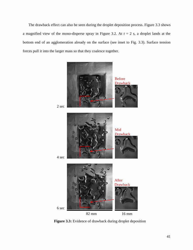
The drawback effect can also be seen during the droplet deposition process. Figure 3.3 shows

a magnified view of the mono-disperse spray in Figure 3.2. At t = 2 s, a droplet lands at the

bottom end of an agglomeration already on the surface (see inset to Fig. 3.3). Surface tension

forces pull it into the larger mass so that they coalesce together.

2 sec

4 sec

6 sec

Figure 3.3: Evidence of drawback during droplet deposition

16 mm

After

Drawback

Before

Drawback

82 mm

Mid

Drawback

42

The area of the substrate covered by the fluid was measured using image analysis software

(ImageJ, National Institute of Health, Bethesda, MD, USA). Since the focus was on the

continuous film, the images were cropped to 740 x 960 pixel resolution leading to an observable

area of 4556 mm2. All droplets and liquid masses with outlines fully visible in the captured area

were counted towards the total area coverage given the fact that, especially in the early frames, it

was hard to distinguish which droplets and liquid masses would end up in the final continuous

liquid film. Figure 3.4 shows the fraction of the observable area covered by the fluid over the 20

second recording time of the camera. The data series represents the average of the three

experimental area fraction values at each time step. The error bars represent the maximum and

minimum values obtained in the three experiments. The area covered grows rapidly up to the 10

second mark at which point the solenoid valve is no longer triggered. Afterwards, only slight

fluctuations in the form of decrease due to drawback or increase due to the settling of the liquid

film on the substrate can be seen.

Figure 3.4: Fraction of observable area covered by fluid over 20 second recording time

0

0.1

0.2

0.3

0.4

0.5

0.6

0 5 10 15 20 25

Ar

ea

Fr

ac

tio

n

Time (seconds)

43

Liquid film growth occurs in the first 10 seconds of the experiments. Eq. 3.1 characterizes

the growth period (first 10 seconds) of the curve in Figure 3.4, namely the average growth of the

liquid film in the three experiments. This equation relates growth of the wetted area to time:

𝐴𝑟𝑒𝑎 𝐹𝑟𝑎𝑐𝑡𝑖𝑜𝑛 = 0.0003𝑡3 − 0.0089𝑡2 + 0.1078𝑡 + 0.0009 (3.1)

Next we calculate the overlap between the droplets deposited (λ). The extent of overlap

between droplets deposited on the surface is described by the dimensionless overlap ratio [22]:

𝜆 = 1 −𝐿

𝐷𝑠 (3.2)

Where, L is the center-to-center distance between the droplets and Ds is the droplet spread

diameter. If the centers of the droplets coincide, then there is complete overlap and λ = 1. For

partial overlap, 0< λ <1 and if there is no overlap λ ≤ 0.

In order to estimate the overlap ratio, the number of droplets deposited must be known which

can be calculated by obtaining the fluid volume deposited on the substrate. To calculate the

volume of the fluid that had been dispensed to form the single continuous sheet (V), the liquid

was collected off the substrate using a syringe after the experimental photograph representing the

equilibrium state at t = 20 min had been taken. Collecting the fluid after 20 minutes on the

substrate did not lead to inaccuracy in the weight value as we had determined in separate

experiments that the evaporation only led to a decrease of 0.37% in the weight of the fluid sheet

over the 20 minutes. The fluid collected was weighed on a balance (AL-204, Acculab, Bradford,

MA, USA) with a resolution of 0.1 mg. The average weight of the liquid from the three

experiments was 4.586 grams. The weight measured in our experiments varied by less than ±2%

of the average value. This weight translates to a volume of 3.75x10-6 m3. Considering the 2.5 mm

44

diameter droplets to be spheres with a volume of 8.18x10-9 m3, we can determine that 458

droplets have landed on the substrate. This is a reasonable estimate since our nozzle has 49 holes

and 10 pulses were applied to the solenoid valve. The volume and droplet number were assumed

to increase linearly with time and reach the final number after 10 seconds.

The overlap ratio calculation will concentrate on the first 10 seconds as the focus is on liquid

film formation. Drawback will not be taken into consideration since the film is forming during

this time period and is constantly evolving. The wetted area (AW) is calculated as the product of

the length (x) and height (y) of the sheet:

𝐴𝑊 = 𝑥 ∗ 𝑦 = [(𝑚 − 1)𝐿 + 𝐷𝑠] ∗ [(𝑛 − 1)𝐿 + 𝐷𝑠] (3.3)

Where, m is the number of droplets in each column of the liquid sheet, n is the number of

droplets in each row of the sheet.

Since the nozzle plate was arranged in a square pattern of 7 holes in 7 rows, the wetted area

can be approximated as a square, in which case n = m and AW reduces to:

𝐴𝑊 = [(√𝑚 − 1)𝐿 + 𝐷𝑠]2 (3.4)

Where, now m represents the total number of droplets deposited.

To predict Ds, the spread factor 𝜉 = 𝐷𝑠

𝐷 is introduced. The droplet spread factor 𝜉 varies with

both impact Weber (We) and Reynolds (Re) numbers as well as the advancing contact angle (βa).

A simple correlation [48], introduced in Chapter 2, can be used to calculate the value of 𝜉 as a

function of these parameters:

45

𝜉 =𝐷𝑚𝑎𝑥

𝐷= √

𝑊𝑒+12

3(1−𝑐𝑜𝑠𝛽𝑎)+4(𝑊𝑒/√𝑅𝑒) (3.5)

Where 𝜉 is the maximum spread factor, Dmax is the maximum spread diameter after impact, D

is the initial droplet diameter and βa is the advancing contact angle. The advancing contact angle

(βa) was set at 90°, which is typical of water on metal surfaces [48]. Plexiglass is hydrophilic and

this advancing contact angle is appropriate. The equilibrium liquid-solid contact angle was 65°.

Since the contact angle was measured at the liquid/substrate interface, this study only applies to

hydrophilic surfaces in which the contact angle is less than 90°. The droplet impact velocity

(𝑈 = √2𝑔ℎ) was calculated to be 1.66 m/s for the 14 cm distance between the nozzle plate and

substrate. The Weber number (𝑊𝑒 = 𝜌𝑈2𝐷/𝜎) for our experiments was calculated to be 133

and the Reynolds number (𝑅𝑒 = 𝜌𝑈𝐷/𝜇) was 41. Substituting these values into Eq. 3.5 gave us

𝜉 = 1.3 and Ds = 3.25 mm. The substrate surface area covered by a single droplet can be

measured from the experiments. The surface area (𝜋𝐷𝑠2/4) of 8.3 mm2 given by this Ds value

agrees well with the surface area measurements in the experiments for a single droplet. The

average of 10 surface area measurements for a single droplet from the experiments was 7.88

mm2. The measurements varied by ±5% of the average value.

Note that Equations 3.2 and 3.4 do not explicitly include surface or liquid properties.

However, the droplet spread diameter (Ds) can either be measured from experiments or

calculated from correlations, similar to Eq. 3.5, that are typically functions of We, Re, and

liquid-solid contact angle. Ds determines both overlap ratio (λ) and wetted area (AW), making

these variables and the models derived using them a function of surface and liquid properties.

Therefore, Eq. 3.2 in conjunction with results in Chapter 2 can be used to predict the rupture or

46

continuity of films constructed in this study from depositing 87 wt% glycerin in water droplets

onto a transparent Plexiglas substrate at ambient temperature.

Knowing the droplet spread diameter (Ds) as well as the number of droplets deposited (m)

and the surface area covered at each time step from the experiments (AW), we can use Equation

3.4 to obtain the variation of droplet center-to-center distance (L) over time as shown in Figure

3.5 and subsequently calculate overlap ratio (λ) from Eq. 3.2 as graphed in Figure 3.6. The

assumption here is that the droplets are falling in a square pattern as described by Equation 3.4.

The average droplet center-to-center distance considering the entire 10 second period and three

experiments is 2.55 mm. This value is obtained by taking an average of the center-to-center

distances calculated at each time step for each experiment. The droplet center-to-center distance

at each time step is calculated via Eq. 3.4 by substituting the appropriate AW and m for that time

step along with Ds = 3.25 mm. Comparing this value to the spacing between the holes on the

nozzle plate of 5 mm, one can state that a droplet landed in-between two droplets coming from

adjacent nozzles due to the randomization caused by the air flow from the fans. The average

overlap ratio considering the entire 10 second period and three experiments is 0.22 which is less

than 1 and means that there is partial overlap between the droplets. Comparing the experimental

images and their accompanying overlap ratios to the critical value of 0.293 reported in Chapter 2,

we can see that indeed continuous films formed once this overlap ratio was surpassed. The

experiment presented in Figure 3.2 has an overlap value of 0.263 at t = 8 s and an overlap value

of 0.313 at t = 10 s. As evident in Figure 3.2, the liquid sheet takes shape in t = 8 s and has a

closed perimeter and by t = 10 s it is fully formed.

47

Figure 3.5: Variation of Droplet Center-to-Center Distance (L) with time

Figure 3.6: Variation of Overlap Ratio (λ) with time

0

0.5

1

1.5

2

2.5

3

3.5

0 2 4 6 8 10 12

Dr

op

let

Ce

nte

r-t

o-C

en

ter

Dis

tan

ce

(m

m)

Time (seconds)

0

0.05

0.1

0.15

0.2

0.25

0.3

0.35

0.4

0 2 4 6 8 10 12

Ov

er

lap

Ra

tio

Time (seconds)

48

Substituting the now known values of number of droplets deposited (m) and droplet center-

to-center distance (L) at each time step and the droplet spread diameter (Ds) of 3.25 mm into Eq.

3.4 we obtain the growth curve in Figure 3.4 with its corresponding growth equation, Eq. 3.1,

validating our procedure. Once again, the volume and droplet number were assumed to increase

linearly with time and reach the final number after 10 seconds.

We can use this analysis to determine the largest continuous square liquid film that can be

achieved for a given volume of fluid. The largest area we can cover with a continuous film (Aw)

for a given volume of fluid (V) can be predicted using Eq. 3.4 considering drawback, 𝜃2𝐷. The

following equation was also presented in Chapter 2 as Eqns. 2.10 & 2.19.

𝐴𝑊 = [𝐷𝑠 + (√𝑚 − 1)𝐿]2

𝜃2𝐷 (3.6)

The largest continuous liquid film is achieved for 𝜃2𝐷 = 1 and λ = 0.293. This corresponds to

the tip of the breakup region presented in Figure 2.8 of Chapter 2.

If we take the experiments presented in this chapter as an example, we had a dispensed

volume of 3.75x10-6 m3. We considered the 2.5 mm diameter droplets to be spheres with a

volume of 8.18x10-9 m3 and therefore determined that 458 droplets had landed on the substrate.

Substituting the number of droplets along with L = 2.3 mm and Ds = 3.25 mm for λ = 0.293 and

𝜃2𝐷 = 1 in Eq. 3.6, we obtain AW = 2517 mm2. This is the largest continuous liquid film

achievable with a dispensed volume of 3.75x10-6 m3 and 2.5 mm diameter droplets. As stated

previously, the actual area that was covered at t = 10 s (m = 458 droplets) averaged 2268 mm2

over the experiments presented in this chapter. This is due to the fact that the overlap ratio here

was λ = 0.33 as previously calculated.

49

If we wanted to know the minimum number of droplets that would be required to form a

continuous liquid film to cover the 2268 mm2 area, we would substitute AW = 2268 mm2 along

with L = 2.3 mm and Ds = 3.25 mm for λ = 0.293 and 𝜃2𝐷 = 1 in Eq. 3.6. This would give us

m = 412 droplets. Considering the fact that we deposited 458 droplets, we can conclude that we

could have achieved a continuous film over the same area by depositing 46 droplets less than we

did in the experiments. This would have changed the overlap ratio between the droplets from

λ = 0.33 to λ = 0.293.

The least number of droplets required to cover a given area is achieved when there is no

interaction between the droplets. The minimum number of droplets that would be required to

cover a 2268 mm2 area can be determined by setting λ = 0 and 𝜃2𝐷 = 1 in Eq. 3.6, along with

values of AW = 2268 mm2, L = 3.25 mm and Ds = 3.25 mm. This calculation gives us m = 215

droplets. We can compare this number with the largest number of non-overlapping circles that

can be packed into a given area, which is 231 droplets for our case [50], as shown in Fig. 3.7.

Figure 3.7: Representative arrangement of maximum number of non-overlapping circles that can

be packed into a square area of 2268 mm2 with Ds = 3.25 mm [50].

50

As mentioned before, substituting the now known values of number of droplets deposited (m)

and droplet center-to-center distance (L) at each time step and the droplet spread diameter (Ds) of

3.25 mm into Eq. 3.4 or Eq. 3.6 with 𝜃2𝐷 = 1, we obtain the growth curve in Figure 3.4 with its

corresponding growth equation, Eq. 3.1, verifying our procedure. Once again, the volume and

droplet number were assumed to increase linearly with time and reach the final number after 10

seconds. This curve is plotted in Figure 3.8 below. As a comparison, the growth curves predicted

by having λ = 0.293 for coverage by a continuous film or λ = 0 for maximum coverage are

plotted as well. The overlap ratio (λ) remains constant for the entire time period of 10 seconds in

these two cases as opposed to the overlap ratio for the experimental case which varies with time.

The observable area was kept similar to the experiments at 4556 mm2. The experimental graph

covers 2269 mm2 after 10 seconds or 0.5 of the observable area, while the continuous film covers

2506 mm2 or 0.55 of the observable area and the maximum area coverage would be 4829 mm2 or

1.06 of the observable area.

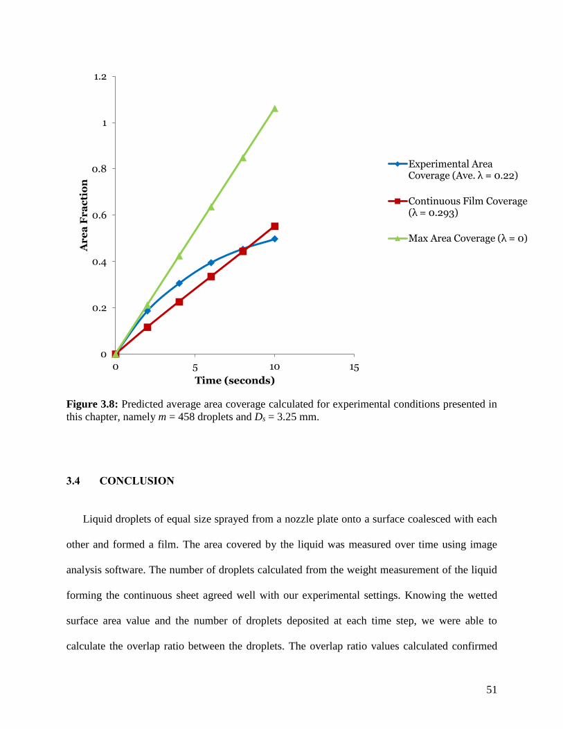
51

Figure 3.8: Predicted average area coverage calculated for experimental conditions presented in

this chapter, namely m = 458 droplets and Ds = 3.25 mm.

3.4 CONCLUSION

Liquid droplets of equal size sprayed from a nozzle plate onto a surface coalesced with each

other and formed a film. The area covered by the liquid was measured over time using image

analysis software. The number of droplets calculated from the weight measurement of the liquid

forming the continuous sheet agreed well with our experimental settings. Knowing the wetted

surface area value and the number of droplets deposited at each time step, we were able to

calculate the overlap ratio between the droplets. The overlap ratio values calculated confirmed

0

0.2

0.4

0.6

0.8

1

1.2

0 5 10 15

Ar

ea

Fr

ac

tio

n

Time (seconds)

Experimental Area Coverage (Ave. λ = 0.22)

Continuous Film Coverage (λ = 0.293)

Max Area Coverage (λ = 0)

52

the findings in Chapter 2 and reaffirmed the fact that λ = 0.293 is significant and continuous

films form once this critical overlap ratio is surpassed whether they are formed using droplet

deposition or mono-disperse sprays. Drawback was also seen both during and after spraying

similar to droplet deposition. Combining the results from this chapter and Chapter 2, the largest

area that can be covered by a continuous liquid film given a volume of fluid was successfully

calculated. This conclusion would greatly assist industries in predicting the amount of paint

required to fully cover a certain surface without the need for trial and error runs thus saving time

and money.

53

CHAPTER 4

FORMATION OF LIQUID SHEETS BY SPRAYING ON A

SURFACE

4.1 INTRODUCTION

Spray droplets impact onto the surface and coalesce; creating large local masses on the

substrate that drawback subsequent droplets causing breakup in the liquid film. The goal of this

chapter of the thesis is to capture and analyze the evolution of liquid masses from a spray over

time. In order to see the outline of the liquid masses, a continuous liquid film is not created and

only a small amount of liquid is dispensed leading to a low overlap ratio which may leave

significant gaps within the film if only a small number of droplets are deposited. Questions to be

answered are: how do interactions between droplets cause a non-uniform liquid film; and what

droplet size distribution and overlap ratio should be utilized in sprays to create a uniform film?

The experiments were conducted using 87 wt% glycerin in water solution. The spray was

deposited onto a Plexiglass substrate and photographed from below.

4.2 EXPERIMENTAL SYSTEM

A schematic of the experimental system devised for spraying 87 wt% glycerin in water

solution is given in Figure 4.1. A tank full of liquid was connected to a centrifugal pump

(PA411-50MT, The Berns Corporation, USA) that passed the fluid through stainless steel and

plastic tubing towards a solenoid valve (8262H232, ASCO Valves, USA). A partially open

54

metering valve (S-1RS6, Swagelok, USA) and a pressure regulator (26A, Watts Water

Technologies., USA) were used to manually control the fluid flow upstream of the nozzle.

Compressed air, controlled by a pressure regulator (3476-A, Matheson, USA), was used to

atomize the fluid properly. Air flow was switched on when required by a second solenoid valve

(RHL206H50B, ASCO Valves, USA). The fluid and pneumatic solenoid valves were normally

closed, and a pulse generator (PDG-2515, Directed Energy, Fort Collins, CO, USA) triggered

transistor switches to open the valves for a precise amount of time. When the valves were

opened, fluid and compressed air passed through a stainless steel air-atomizing round spray

nozzle (Model 1/8JJ–SS+SUJ11–SS, Spraying Systems Co., Wheaton, IL, USA) for 1.5 s. The

fluid pressure was kept constant at 240 kPa and the air pressure at 150 kPa. The mean diameter

of the droplets (d10) for this spray was measured using a PDPA system (TSI, Shoreview, MN,

USA) and determined to be 242 µm.

The transparent Plexiglas substrate was placed 27 cm below the spray nozzle and a high

speed camera (FASTCAM SA5, Photron, San Diego, CA, USA), placed under it, pointing

upwards, to record spray impact. Videos were taken at 4000 frames per second, 1024x1024 pixel

resolution and 249.8 µs shutter speed.

55

Figure 4.1: Schematic of the 87 wt% glycerin spray experimental setup

The spray is mounted on a fixture consisting of four interconnected 6-feet high aluminum

T-beams that hold two surfaces via mount brackets. A picture of the spray fixture is provided in

Figure 4.2. The surfaces are 100 cm in length and 50 cm in width. One surface hosts the spray

setup and the other contains the substrate. The mount brackets come with screws that can be

loosened to allow for the repositioning of the surfaces. Therefore, the substrate can be moved

relative to the spray nozzle. The substrate is held down by a stainless steel threaded ring and

holder that allows for the changing of the substrate with ease. The fixture has leveling legs on

either end of the T-beams that allow for the entire frame to be flipped over so that the position of

the spray and substrate surfaces is reversed. In this manner inverse spraying is achieved. The

frame allows for the positioning of the light and camera such that video can be taken from both

above and below the substrate. The spray nozzle is held in place by a mounting plate which has

fittings for both the showerhead and the air-atomizing round spray nozzle.

56

Faceplate securing

spray nozzle

Substrate Holder

Spray Holder

57

Figure 4.2: Picture of spray fixture. Fixture has adjustable brackets at the four corners.

4.3 RESULTS & DISCUSSION

Figure 4.3 illustrates the deposition of spray droplets onto the transparent Plexiglas substrate,

viewed from below. The spray was switched on at t=0 and turned off at t=1.5 s. Small droplets

were evident on the surface (t=0.3 s), which grew larger as more droplets were deposited and

amalgamated with the existing liquid on the surface. By t=1.4 s there were relatively large

masses of liquid on the surface. The spray stopped at t=1.5 s and no additional liquid was

deposited after that time. The irregular liquid masses continued to move and become more round

(see t=2.6 to 5.1 s), so that the surface area covered by liquid was reduced.

Stainless steel threaded

ring and holder

58

0.3 s 0.4 s 0.5 s 0.6 s

1.4 s 2.6 s 3.3 s 5.1 s

Figure 4.3: Accumulation of spray droplets on the substrate

Figure 4.4 shows the variation in the area of surface covered by liquid, as measured from

photographs using image analysis software. Two different curves are shown, for the total area

covered by “small” arbitrarily defined as those with area ≤1 mm2 and “large” (area>1 mm2)

patches of liquid. Immediately after the spray was turned on the area covered by small regions of

liquid increased until t≈0.5 s. By this time many of the smaller spots of liquid had grown larger

than 1 mm2, and therefore the curve in Figure 4.4 slopes downwards, while that showing area

covered by large spots increases. At t=1.5 s the spray was shut off. Further changes in the area

covered by liquid were because of merging of droplets on the surface and drawback. The total

area covered by liquid increased briefly due to merging of small droplets, and then decreased as

smaller droplets were pulled into larger ones. The area covered by smaller masses of liquid

Spray Stops-1.5 s

2

3 m

m

59

remained approximately constant. These represent small, isolated droplets that did not contact

any other liquid and remain undisturbed.

Figure 4.4: The time evolution of areas during and after spraying

Figure 4.5 shows details of how small droplets coalesced with larger liquid masses on the

surface. At t=518 ms a small portion of the substrate is shown enlarged. At t=519 s a droplet

landed in that area, connecting several of the smaller liquid patches on the surface. Surface

tension forces drew the smaller droplets towards the larger mass (t=528 ms) then pulled the

coalesced droplets into a more circular area (t=745 ms).

0

50

100

150

200

250

300

350

400

0 0.5 1 1.5 2 2.5 3 3.5 4 4.5 5 5.5

Ar

ea

(m

m2)

Time (seconds)

≤ 1 mm^2

> 1 mm^2

Total Area

Sp

ra

y S

top

s Drawback

≤1 mm2

>1 mm2

Total Area

60

518 ms 519 ms 528 ms

598 ms 668 ms 745 ms

Figure 4.5: Coalescence and drawback in spray droplets

Coalescence and movement of the liquid on the surface persisted well after the spray was

shut off. Figure 4.6 shows a section of the surface for t > 1.5 s, when no more liquid was being

deposited on the surface. In the region marked with a square, two pools of liquid that were

initially separate (t=1.53 s) moved due to surface tension driven flows and touched each other

(t=1.65 s). The smaller region of liquid was pulled into the larger one (t=1.90 s) until they

formed a single mass (t=2.15 s).

1.9

mm

61

1.53 s 1.65 s

1.90 s 2.15 s

Figure 4.6: Coalescence and drawback in spray droplets after the spray is shut off

To understand how droplets deposited by a spray onto a solid surface are driven to coalesce,

a series of tests were done where the coalescence of two sequentially deposited droplets onto a

flat substrate was observed, while varying the center-to-center distance and the volume ratio of

the two droplets. The droplet generator described in Chapter 2 was used to conduct these

experiments. A summary of the results and the mechanism behind droplet coalescence will be

provided here and further details and results can be found in [51].

A schematic of the coalescing droplets is presented below in Figure 4.7. The droplets are

assumed to be formed by the impact of two initially spherical droplets with radii r1 and r2

23 mm

62

respectively. The droplets rest on the substrate with liquid-solid contact angle 𝜃. Once on the

substrate, the coalescing droplets are essentially two overlapping spherical caps.

Figure 4.7: A side view of equilibrium spreading diameter of each droplet (𝐷𝑠1 , 𝐷𝑠2), spreading

diameter, 𝐷𝑥, droplet center-to center distance, 𝐿, contact angle, 𝜃.

The rate at which droplets are pulled towards each other depends on the volume ratio. To

study this effect [51], the volume ratio of the droplets was changed, but the overlap ratio between

them was kept constant. The sessile droplet placed on the substrate was 2 or 3 times larger in

volume than the impacting droplet. Initially, the droplets were driven outwards due to the high-

pressure region near the edges of the droplets. Afterwards, a liquid bridge formed between the

droplets as they coalesced that was concave upwards, while the droplets were convex upwards.

The Young-Laplace equation states that the pressure difference across any free surface is [51]:

∆𝑝 = 𝜎𝜅 (4.1)

Where 𝜎 is the liquid surface tension and 𝜅 the curvature of the surface. The pressure in the

droplet will be higher than the surroundings if the curvature is positive (convex upwards).

𝒓𝟐 𝒓𝟏

𝑳

𝑫𝒔𝟐 𝑫𝒔𝟏

𝑫𝒙

𝜽 𝜽

63

However, if the curvature is negative (concave upwards) the pressure will be negative.

Therefore, the driving force for coalescence was the positive pressure inside the bulk of the two

droplets and the negative pressure in the liquid bridge connecting them. From particle image

velocimetry images of coalescing droplets it is clear that flow is directed from the periphery of

the drops towards their center [26].

Increasing the volume of the sessile droplet reduced its curvature, and therefore the pressure

inside it. As a result, the pressure difference between the two droplets became larger and they

were driven to each other more quickly.

As [51] details, the rate at which droplets are pulled towards each other also depends on the

overlap ratio. To study this effect, the overlap ratio between the droplets was changed, but the

volume ratio was kept constant. The sessile droplet was 3 times larger in volume than the

impacting droplet. For low overlap ratio, negative pressure was observed in the liquid bridge

between the two droplets. Once again, as in the case for the varying volume ratio, the pressure

difference between the two droplets pulled them together, leading to a large displacement of the

edges. As the overlap ratio was increased, the curvature of the combined droplet quickly became

uniform and no pressure difference was observed between the different regions of the liquid and

the coalesced droplet remained more or less stationary.

Viewing droplet coalescence from an energy perspective, it is clear that the process reduces

the surface area and therefore surface energy is minimized. The surface area of the combined

(coalesced) droplet is smaller than that of the individual droplets before coalescence.

64

4.4 CONCLUSION

Liquid droplets sprayed on a surface coalesce with each other to form local liquid pockets,

preventing the formation of a continuous uniform film. In the early time period of spraying, the

liquid mass on the surface is comprised of numerous small pockets. As time passes, the droplets

on the substrate coalesce with one another and the majority of liquid mass on the surface consists

of large liquid islands. Drawback occurs throughout the spraying process and is especially

evident after spraying is over. Smaller droplets (or liquid masses) get pulled into adjacent larger

droplets (or liquid masses). As the liquid patch size grows, the process accelerates and it draws in

any smaller droplets faster. Liquid motion is driven by pressure difference between the droplets.

The liquid bridge that connects two coalescing droplets has a negative curvature, leading to a

negative pressure in it, while both droplet surfaces have positive curvature and therefore a

positive pressure. This pressure difference creates a flow in both droplets from the edges towards

the center (the liquid bridge) making them coalesce. A greater difference in the volume of the

droplets causes a larger curvature difference and therefore pressure imbalance. Also, the larger

the center-to-center distance between the two drops (smaller overlap), the greater the pressure

difference driving the two drops together. Therefore, to obtain a uniform film, either the spray

droplet size distribution should be uniform so that the volume ratio of the droplets dispensed is

kept to a minimum or the overlap ratio between the droplets should be increased so that they

remain static after deposition. To obtain a uniform thin film, the sprayed droplets should be small

and close to one another.

65

CHAPTER 5

BUBBLE ENTRAPMENT AND ESCAPE FROM

SPRAYED PAINT FILMS

5.1 INTRODUCTION

Bubble entrapment is one of the major defects affecting the quality of the finished paint

coating on cars. It is standard practice in the automotive paint industry to wait for 5-10 minutes

after spraying a component, a period known as the “flash-off” time during which some of the

solvent evaporates, before placing it in an oven to cure [29]. This delay is known to minimize the

number of bubbles and suppress their growth, but the exact mechanism by which bubbles leave

the paint has not been established.

This study was undertaken to determine how air bubbles escape from a spray painted film.

We photographed the motion of bubbles in liquid films applied by spraying paint onto a glass

substrate. A model paint, whose surface tension and viscosity were measured, was used. All

experiments were done at room temperature. The size and number of bubbles was measured as a

function of time using image analysis software. Substrates were weighed to determine the rate of

solvent evaporation. An analytical model of solvent diffusion through the paint layer was used to

calculate concentration gradients and thereby to estimate the magnitude of surface tension

gradients that drive Marangoni flows in the paint.

66

5.2 EXPERIMENTAL SYSTEM

Experiments were conducted using model paint, prepared by mixing 85 wt% resin with 15

wt% solvent. The resin consisted of 70 wt% CYMEL 1159 (Cytec Industries Inc., Woodland

Park, NJ, USA) and 30 wt% PARALOID AT400 (Dow Chemical Co., Midland, Michigan,

USA). The solvent used was n-Butanol (Caledon Laboratory Chemicals, Georgetown, ON,

Canada). Using thermogravimetric analysis (TGA) it was determined that the pure resin initially

contained 35.7 wt% solvent. The initial solvent concentration in the model paint was therefore 45

wt%. The surface tension and viscosity of the paint were measured experimentally by Javaheri

[52] using a digital viscometer (DV-I, Brookfield Engineering Laboratories, Middleboro, MA,

USA). The viscosity was measured for the pure resin mixture (Cymel and Paraloid) and then for

solutions of the resin in n-butanol in 2 wt% increments up to 20 wt% of solvent (Fig. 5.1a). The

viscosity decreased from approximately 3500 cP for the pure resin to 200 cP for a solution with

20 wt% butanol. The surface tension was measured [52] using a force tensiometer (Sigma KSV,

Biolin Scientific, Stockholm, Sweden) with a standard platinum-iridium ring in contact with the

model paint. Increasing amounts of the solvent were added to the paint similar to what was done

when measuring viscosity. The surface tension decreased from 27.5 mN/m for pure resin to 23.5

mN/m for pure n-butanol (Fig. 5.1b). The model paint, consisting of resin with 15% solvent, had

density (𝜌) of 988 kg/m3, volatile partial density (𝜌𝑣) of 442 kg/m3, dynamic viscosity (µ) of 240

cP and surface tension (σ) of 26 mN/m. As solvent concentration decreased, the viscosity and

surface tension of the model paint increased. Properties of n-butanol were taken from [53].

67

(a) Viscosity

(b) Surface Tension

Figure 5.1: Change in (a) viscosity and (b) surface tension of model paint with variation of

solvent concentration. The data for these graphs were provided by Javaheri [52].

0

500

1000

1500

2000

2500

3000

3500

4000

0 2 4 6 8 10 12 14 16 18 20

Vis

co

sit

y (

cP

)

Solvent Concentration (%Weight)

23

24

25

26

27

28

0 10 20 30 40 50 60 70 80 90 100

Su

rfa

ce

Te

ns

ion

(m

N/m

)

Solvent Concentration (%Weight)

68

Figure 5.2 shows a picture of the experimental system. A handheld compressed air sprayer

(Project Sprayer, Wagner Spray Tech, Plymouth, MN, USA) was used to spray model paint onto

the substrate. The substrate was a 2”x 2” piece of heat-resistant borosilicate glass (8476K121,

McMaster-Carr, Elmhurst, IL, USA), which was chosen because it was transparent and allowed

bubbles to be clearly seen when illuminated from below. The compressed air sprayer was used to

spray model paint onto two glass substrates at the same time: one substrate was used to

photograph bubble motion and the other to measure weight losses. The sprayer was moved at a

constant speed across the substrate surface, keeping the spray pattern and flow rate constant

throughout the experiments. The number of passes of the spray gun over the substrate determined

the paint film thickness. A single pass of the sprayer deposited a paint thickness of

approximately 75-100 µm, so 1 to 6 passes were used in experiments. A balance (AL-204,

Acculab, Bradford, MA, USA) was used to measure the weight of the substrate before and after

spraying with a resolution of 0.1 mg and the weight of the paint calculated from the difference.

The average paint thickness was calculated by dividing the paint mass by the density of the paint

and the surface area of the test surface. The uncertainty in average thickness with this method

was estimated to be less than ±1 µm.

After spraying paint, the glass substrate was placed horizontally above a LED light panel

(Gagne Inc., Johnson City, NY, USA) that provided backlighting. It took approximately a minute

to remove the substrates from the paint booth, position them under the camera and start

photographing and as such time t = 0 marks the first photograph taken. Still images were taken at

5 s intervals for 15 minutes using a digital SLR camera (D90, Nikon Inc., Melville, NY, USA)

mounted above the substrate, pointing downward and triggered by a programmable timer (TC-

N3, JYC Technology, Hong Kong, China). The images were taken at 4288x2848 pixel

69

resolution. The pictures were analyzed using the threshold function in image analysis software

(ImageJ, National Institute of Health, Bethesda, MD, USA) to count the number of bubbles in

each image and the cross-sectional area of each bubble. Thresholding (Binary Contrast

Enhancement) sets a grayscale cutoff point and uses it to transform a grayscale image to binary

(black and white). Grayscale values below the limit become black and those above become

white. Thus after thresholding, bubbles may no longer look perfectly circular and have a rather

jagged outline. The figures shown in this chapter are the experimental photographs after

thresholding.

ImageJ software does have limitations when it comes to distinguishing the individual bubbles

in the early time intervals where there is clustering and a large number of bubbles are present in

the paint film. This issue was mitigated through enhancing the contrast of the experimental

images before thresholding and also fine-tuning the grayscale cutoff point to ensure that the

figures produced after the threshold process closely resembled the experimental figures. The

smallest bubbles resolved through this process had a diameter of 4 µm which corresponds well

with the 5 µm value seen in literature for bubbles entrapped from viscous droplet impact onto a

glass substrate [34].

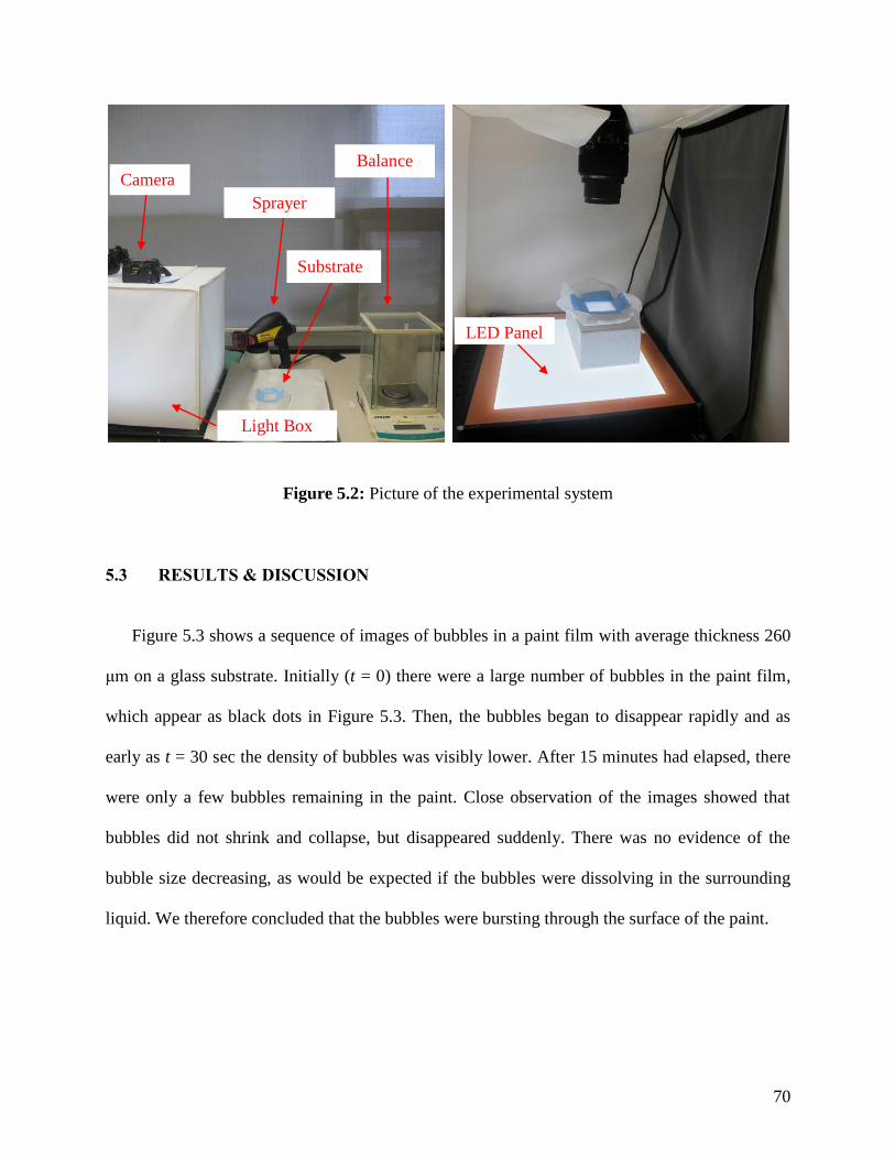
70

Figure 5.2: Picture of the experimental system

5.3 RESULTS & DISCUSSION

Figure 5.3 shows a sequence of images of bubbles in a paint film with average thickness 260

μm on a glass substrate. Initially (t = 0) there were a large number of bubbles in the paint film,

which appear as black dots in Figure 5.3. Then, the bubbles began to disappear rapidly and as

early as t = 30 sec the density of bubbles was visibly lower. After 15 minutes had elapsed, there

were only a few bubbles remaining in the paint. Close observation of the images showed that

bubbles did not shrink and collapse, but disappeared suddenly. There was no evidence of the

bubble size decreasing, as would be expected if the bubbles were dissolving in the surrounding

liquid. We therefore concluded that the bubbles were bursting through the surface of the paint.

Balance

Sprayer

LED Panel

Camera

Substrate

Light Box

71

0 min 15 sec

30 sec 45 sec

2 min 4 min

11 min 15 min

Figure 5.3: Bubbles in 260 μm thick paint film

17 mm

72

Figure 5.4 shows the change of bubble density (the number of bubbles per square millimeter)

for paint films with varying thickness (L). The initial bubble count was approximately the same,

approximately 50 bubbles/mm2 for all the films, even though the thinnest layer was formed using

a single pass of the spray while the thickest took up to 6 passes. It is likely that bubbles created

in subsequent passes merged with those already on the surface during the first pass of the paint

spray. It is also possible that in the thickest paint layers, bubbles in the top layers obscured other

bubbles below them. The bubble density decreased very rapidly for the thinnest film (L=100

μm), decreasing to 10% of its initial value in 100 s and almost 0 in less than 500 s. As the film

thickness increased the bubbles took longer to escape from the film, but in all cases most bubbles

had left by t = 900 s. In the thickest film (L=450 µm) there was a large amount of movement of

the paint film so that new bubbles moved into the field of view during the initial 100 s, leading to

fluctuations in the bubble density. The variation may also be due to bubbles at varying depths in

the paint moving past each other.

Figure 5.4: Change in bubble density with time for paint films of varying thickness

0

10

20

30

40

50

60

0 100 200 300 400 500 600 700 800 900 1000

Bu

bb

le c

ou

nt

pe

r m

m2

Time (seconds)

100 um

150 um

260 um

450 um

73

To define an average bubble size, the Sauter Mean Diameter (SMD), d32, was calculated,

defined as the diameter of a bubble that has the same volume to surface area ratio as the total

group of bubbles being observed. Image analysis was used to measure bubble diameter (d),

which ranged from 4 to 650 µm in diameter. As [34] reports, the bubbles entrapped from viscous

droplet impact onto a glass substrate ranged from 5 to 50 µm in diameter, with the average size

increasing linearly with radial distance from impact center. In our experiments, the larger

bubbles observed were due to bubble coalescence during multiple passes of the spray and also

after spray application due to liquid motion. The largest bubbles had diameters greater than the

film thickness, implying that they protruded above the film surface. The SMD was derived from:

𝑑32 =∑ 𝑑3

∑ 𝑑2 (5.1)

Figure 5.5 shows the variation of SMD with time in four different paint films with increasing

thickness. The initial SMD (t = 0) increased with film thickness, suggesting that bubbles merged

with each other during consecutive passes of the paint spray. The SMD decreased with time for

films 260 µm and less in thickness, while it increased for the 450 µm thick film. For the thinnest

films (L=100 µm and 150 µm) the SMD was approximately the same as the film thickness at the

start and then decreased as the largest bubbles broke through the surface and disappeared. There

was relatively little movement of the bubbles in the plane of the paint layer for thin films. For the

450 µm thick film bubbles were seen to be in constant motion, colliding with each other and

coalescing, producing a continuous increase in average bubble diameter.

The thinnest paint film, formed by a single pass of the paint sprayer, best represents at time

t=0 the size of bubbles formed in the absence of any bubble coalescence. We can place an upper

limit on the density of bubbles if we consider a 1 mm x 1 mm square covered by 50 equal-sized

74

circles, corresponding to the highest bubble density seen in Fig. 5.4. The largest diameter of

circles that can be fitted in this area is 143 µm, in which case they cover 80% of the total area

[50]. This number is only a little larger than the mean diameter of bubbles in the thinnest paint

film (L=100 µm). It is likely that when multiple passes of the paint spray are applied the bubble

density in the first layer is already so high that subsequently deposited bubbles collide with each

other and coalesce. The bubble density therefore remains constant while the mean bubble size

increases.

Figure 5.5: Change in Sauter Mean Diameter (SMD) of bubbles with time for paint films of

varying thickness

Bubble velocities in the paint film were measured using a particle image velocimetry (PIV)

plugin for ImageJ [54] that measures the distance travelled by objects in sequential images.

Average velocities were calculated by dividing the displacement of bubbles by the time interval

(5 s) between frames. Figure 5.6 shows the variation of average bubble velocity with time for

0.00

0.05

0.10

0.15

0.20

0.25

0.30

0.35

0.40

0.45

0.50

0 100 200 300 400 500 600 700 800 900 1000

Sa

ute

r M

ea

n D

iam

ete

r (

mm

)

Time (seconds)

100 um

150 um

260 um

450 um

75

films of varying thickness. In thin films the velocity was low and reduced quickly: the velocity in

the L=100 µm film reduced from 3 µm/s to 1 µm/s in 20 s while the velocity in the L=260 µm

film went from 5 µm/s to 1 µm/s in 900 s. The behavior of bubbles in the L=450 µm thick film

was different: the velocity was an order of magnitude greater and it increased for the first 100 s,

reaching a peak of almost 30 µm/s and then gradually decreased to 4 µm/s after 900 s.

The relatively rapid motion of bubbles in the 450 µm thick film, compared to those in the

thinner films, explains why the mean bubble diameter increases in that film. It was observed that

bubbles collided with each other and coalesced, decreasing their number but increasing their

size. In the thinner films bubbles moved much more slowly and collided less frequently. The

mean bubble diameter in thinner paint films is therefore determined by the rate at which bubbles

escape from the surface of the paint film.

Figure 5.6: Change in film and bubble velocity over time for paint films of varying thickness

0.0

0.1

1.0

10.0

100.0

0 100 200 300 400 500 600 700 800 900 1000

Ve

loc

ity

(µ

m/s

)

Time (seconds)

100 um

150 um

260 um

450 um

76

The most obvious reason for bubbles to rise to the surface of an upward facing liquid film is

due to buoyancy forces lifting them up in which case their acceleration is given by the solution to

the force balance equation [55]:

4

3𝜋𝑟3 (𝜌𝑝 +

𝜌

2)

𝑑𝑈

𝑑𝑡=

4

3𝜋𝑟3𝑔𝛥𝜌 − 6𝜋µ𝑟𝑈 − 6𝑟2√𝜋𝜌µ ∫

�̇�(𝑠)𝑑𝑠

√𝑡−𝑠

𝑡

0 (5.2)

Where r is the bubble radius, U is the bubble velocity, 𝜌𝑝 and 𝜌 are the density of the bubble

and liquid respectively, 𝛥𝜌 is the difference between the liquid and bubble density, µ is the fluid

viscosity and 𝑔 is the gravitational acceleration. The term on the left hand side of the equation

includes the “virtual mass” of the liquid that has to be accelerated along with the bubble. The

first term on the right hand side of the equation is the buoyancy force that lifts the bubble

upwards and varies with r3. The second term is Stokes drag and the third is the “Basset force”

which is caused by the development of a wake behind a particle accelerating in a fluid [56].

These last two terms, which retard bubble motion, are proportional to r and r2 respectively. If

there is an assortment of bubbles with varying sizes in a liquid the larger bubbles will rise faster

than the smaller bubbles since the buoyancy term dominates.

To test predictions from this equation experimentally, transparent glass vials, 20 mm in

diameter and 60 mm high, were filled three-quarters full with model paint and shaken to generate

air bubbles within the liquid. The vials were then placed on a level surface and the rise of the

bubbles recorded using a high speed camera (FASTCAM SA5, Photron, San Diego, CA, USA)

at 60 frames per second. Bubbles with diameters ranging from 250 µm to 500 µm had average

velocities from 100 µm/s to 200 µm/s respectively, about the order of magnitude predicted by

Equation 5.2, and it was confirmed that larger bubbles rise faster than smaller ones. However, at

77

these velocities all the bubbles should traverse even the thickest paint film (450 µm) and escape

in a few seconds, whereas many remain in the paint films for over 15 minutes as seen in Fig. 5.3.

Bubbles that rise to the surface of the paint remain trapped there and cannot break through

the interface. Figure 5.7 shows a photograph of the paint-air interface inside a vial in which the

bubbles had been given sufficient time to rise to the surface. The largest bubbles arrived first at

the liquid-air interface and clustered there but were not able to break through. As a bubble

approaches an interface, a thin liquid film remains on its upper surface, which has to drain and

rupture before the bubble can escape as shown schematically in Figure 5.8 [57, 58, 59]. This is

the reason that we can observe bubbles in paint films with diameters greater than the average

film thickness. The time for the bubble to escape becomes greater with increasing liquid

viscosity and decreasing surface tension [58, 59]. Since the paint has high viscosity and

relatively low surface tension, the time for the liquid film to drain will be very long. It is

therefore likely that the larger bubbles rise first to the surface of the paint film, but then remain

trapped there until the film on their surfaces either drains or the bubbles are pushed out by the

movement of the liquid.

Figure 5.7: Bubbles resting at the phase interface (model paint-air) before escaping

19 mm

78

Figure 5.8: Thin liquid film between the bubble and the interface

If bubble escape is driven by liquid movement rather than buoyancy forces alone it should be

possible for bubbles to escape from a downward facing surface as well. To determine whether

bubbles can escape from the paint film even when buoyancy forces oppose their movement we

did tests in which the test surface was turned over after spraying so that the paint film on it was

facing downwards. Figure 5.9 shows photographs of two paint films of approximately the same

thickness (L=150 μm), one facing upwards and the other facing downwards, for two minutes.

Time t = 0 marks the first photograph, but it took approximately a minute to remove the

substrates from the paint booth, position them under the camera and start photographing. The

starting point was therefore not identical – the bubbles on the downward facing substrate were

larger than those on the upward facing one. The bubble density of both films decrease with time.

However, the bubbles on the downward facing surface are visibly larger than those on the

upward facing surface.

Drainage Drainage

Free Surface

Air

Liquid

Liquid Film

Bubble

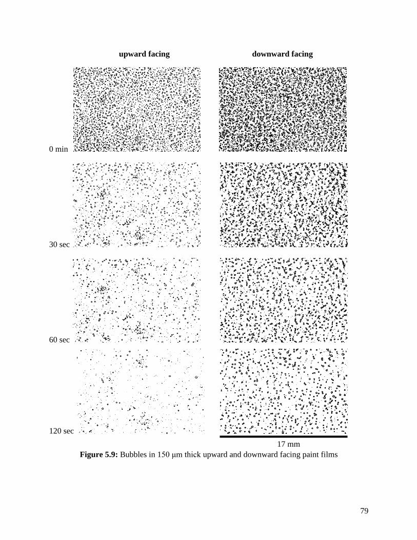
79

upward facing downward facing

0 min

30 sec

60 sec

120 sec

Figure 5.9: Bubbles in 150 μm thick upward and downward facing paint films

17 mm

80

Figure 5.10 shows the variation of bubble SMD with time for both upward and downward

facing paint layers. The SMD of bubbles in a downward facing film was larger than those in an

upward facing film, but both decreased with time. Bubbles therefore escape from the paint even

when buoyancy forces oppose their rise toward the free surface. Liquid motion alone is adequate

to carry bubbles to the surface of a paint film and push them out. In an upward facing substrate

buoyancy forces reinforce this movement, carrying larger bubbles faster to the paint surface and

leaving behind smaller bubbles. In a downward facing substrate buoyancy forces oppose bubble

escape, preferentially lifting larger bubbles towards the substrate while allowing smaller bubbles

to escape.

Figure 5.10: Change in Sauter Mean Diameter (SMD) of bubbles with time for 150 μm thick

upward and downward facing paint films

0.00

0.05

0.10

0.15

0.20

0.25

0 100 200 300 400 500 600 700 800 900 1000

Sa

ute

r M

ea

n D

iam

ete

r (

mm

)

Time (seconds)

upward facing

downward facing

81

Liquid motion in the paint layer is driven by surface tension gradients created by variations

in solvent concentration [60]. Figure 5.11 illustrates this mechanism. When butanol evaporates

from the paint, random fluctuations in the evaporation rate at different points on the surface will

produce surface tension gradients, since surface tension decreases with higher solvent

concentration. The liquid flows from regions of lower surface tension to those of higher surface

tension and create convection cells. These Marangoni flows bring fresh paint from the bottom of

the paint layer to the surface, producing greater concentration gradients along the surface. The

convective flows also carry bubbles to the paint surface and allow them to break through the

surface of the liquid.

Figure 5.11: Bubble escape mechanism

To test whether bubbles can escape from a thin viscous film in the absence of any Marangoni

flows we did a set of experiments in which 87 wt% glycerin in water solution with a viscosity of

124 cP, density of 1224 kg/m3 and surface tension of 63.5 mN/m was sprayed onto the substrate.

The substrate was then photographed at 1 minute intervals for 28 minutes. Figure 5.12 shows

measurements of bubble count as a function of time for a 3 mm thick film. We observed no

change in the bubble count or observe any movement of bubbles or the liquid. The insets to

82

Figure 5.12 are photographs taken at 0, 10 and 25 minutes. The glycerin in water mixture has

values of viscosity, density and surface tension the same order of magnitude as that of the paint.

The main difference between the two is that the paint is much more volatile, containing butanol

solvent that evaporates rapidly. In the absence of a volatile component there are no flows in the

glycerin-water mixtures.

Figure 5.12: Bubble density for 87 wt% glycerin film

Marangoni convection is driven by surface tension forces, which are opposed by viscous

forces. The magnitude of surface tension forces due to concentration gradients can be estimated

by:

𝐹𝜎 =𝜕𝜎

𝜕𝐶.

𝜕𝐶

𝜕𝑥. 𝐿2 (5.3)

Where the film thickness, L, is used as a length scale.

0

0.5

1

1.5

2

2.5

0 200 400 600 800 1000 1200 1400 1600 1800

Bu

bb

le c

ou

nt

pe

r m

m2

Time (seconds)

0 min 10 min 25 min

83

Viscous shear forces that oppose fluid flow can be estimated from:

𝐹𝜇 = 𝜇 𝜕𝑢

𝜕𝑥. 𝐿2 (5.4)

There is no imposed velocity in this problem, but we can define a diffusive velocity with

magnitude u ~ Dv /L. Assuming x~L and substituting into Equation 5.4:

𝐹𝜇 = 𝜇 𝐷𝑣 (5.5)

The Marangoni number (Ma) is the ratio of surface tension to viscous forces [61]:

𝑀𝑎 =𝐹𝜎

𝐹𝜇= (

𝜕𝜎

𝜕𝐶) (

𝜕𝐶

𝜕𝑥) 𝐿2/𝐷𝑣𝜇 (5.6)

Flows in the paint film commence when surface tension forces overcome viscous forces and

the Marangoni number exceeds a critical value. The paint viscosity (µ) and surface tension

variation with concentration (𝜕𝜎/𝜕𝐶) have been measured experimentally (Fig. 5.1). To evaluate

Ma we need to determine the concentration gradient in the film (𝜕𝐶/𝜕𝑥) and the diffusivity of

solvent in the paint layer (Dv).

Solvent transport was modelled by using the 1-D mass transfer model [62, 63] in which

paint is assumed to be a binary mixture in which solvent diffuses through a non-volatile layer.

The paint film was assumed to be a uniform layer of thickness L (Fig. 5.13) in which the butanol

concentration C(x,t) varies with distance from the substrate (x) and time (t). The initial

concentration Ci is uniform and the concentration in the surrounding atmosphere C∞ is zero [63].

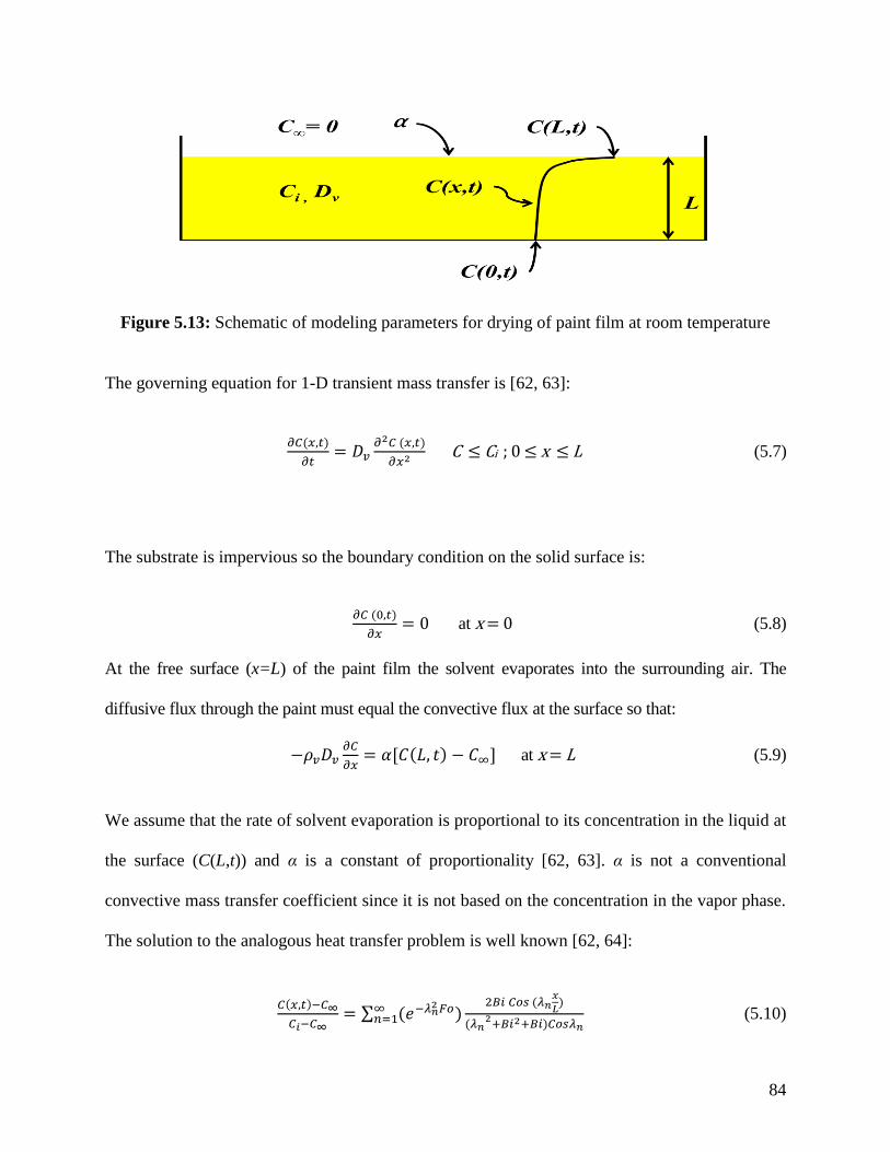
84

Figure 5.13: Schematic of modeling parameters for drying of paint film at room temperature

The governing equation for 1-D transient mass transfer is [62, 63]:

𝜕𝐶(𝑥,𝑡)

𝜕𝑡= 𝐷𝑣

𝜕2𝐶 (𝑥,𝑡)

𝜕𝑥2 C ≤ Ci ; 0 ≤ x ≤ L (5.7)

The substrate is impervious so the boundary condition on the solid surface is:

𝜕𝐶 (0,𝑡)

𝜕𝑥= 0 at x = 0 (5.8)

At the free surface (x=L) of the paint film the solvent evaporates into the surrounding air. The

diffusive flux through the paint must equal the convective flux at the surface so that:

−𝜌𝑣𝐷𝑣𝜕𝐶

𝜕𝑥= 𝛼[𝐶(𝐿, 𝑡) − 𝐶∞] at x = L (5.9)

We assume that the rate of solvent evaporation is proportional to its concentration in the liquid at

the surface (C(L,t)) and α is a constant of proportionality [62, 63]. α is not a conventional

convective mass transfer coefficient since it is not based on the concentration in the vapor phase.

The solution to the analogous heat transfer problem is well known [62, 64]:

𝐶(𝑥,𝑡)−𝐶∞

𝐶𝑖−𝐶∞= ∑ (𝑒−𝜆𝑛

2 𝐹𝑜)2𝐵𝑖 𝐶𝑜𝑠 (𝜆𝑛

𝑥

𝐿)

(𝜆𝑛2+𝐵𝑖2+𝐵𝑖)𝐶𝑜𝑠𝜆𝑛

∞𝑛=1 (5.10)

85

Where,

Eigenvalues λn: 𝜆𝑛 = 𝐵𝑖 𝐶𝑜𝑡 𝜆𝑛 (5.11)

Fourier number: 𝐹𝑜 =𝐷𝑣𝑡

𝐿2 (5.12)

Biot number: 𝐵𝑖 =𝛼𝐿

𝐷𝑣𝜌𝑣 (5.13)

We calculated the proportionality constant α from the value of mass flux, J, using the

equation:

𝐽 = 𝛼(𝐶(𝐿, 0) − 𝐶∞) = 𝛼𝐶𝑖 (5.14)

The surface mass flux of solvent from the paint was measured by recording the weight loss of

paint films of different thickness. Figure 5.14 shows the mass loss from paint films of varying

thickness due to evaporation of solvent, as a percentage of the initial mass. The mass loss

depends on film thickness, and is fastest for the thinnest film (100 μm). Dividing the mass lost

over a 60 second period by the surface area of the film and the time interval yields the volatile

mass flux, J. The value of α was obtained from the average of the mass flux values for the first 3

minutes assuming that the surface concentration remained constant at C(L,0) = 𝐶𝑖 = 0.45. We

calculated an average value of α = 7.4 x 10-5 kg/m2s, which did not vary significantly with film

thickness. In the range of films tested in our experiments α varied by less than ±6% of the

average value.

86

Figure 5.14: Weight loss as a function of time for paint films of varying thickness

The cumulative solvent mass that has escaped from the paint film at time t, Mt, can be

expressed as a fraction of the total solvent mass, M∞, as follows [62]:

𝑀𝑡

𝑀∞= 1 − ∑ (e−𝜆𝑛

2𝐹𝑜∞

𝑛=1)

2𝐵𝑖2

𝜆𝑛2(𝜆𝑛

2+𝐵𝑖2+𝐵𝑖) (5.15)

Figure 5.15 illustrates the mass of solvent that evaporated from the paint film during the

experiments divided by the total solvent mass as a function of √𝑡/𝐿. The analytical solution

assumes a constant Dv and α. If Dv and α are constant then theoretically all the curves in Figure

5.15 should collapse onto a single line. However, in reality, the effective diffusivity could change

over time as the paint dries and a high viscosity film forms on the surface of the paint [62]. The

thinner a paint film is, the faster it will dry and the length of time for which we can assume a

constant diffusivity is reduced. If we assume curves in Figure 5.15 are coincident for √𝑡

𝐿< 6.7 x

40

50

60

70

80

90

100

0 100 200 300 400 500 600 700 800 900 1000

% W

eig

ht

Time (seconds)

100 um

150 um

260 um

450 um

87

104 s0.5/m., then the assumption of constant Dv is reasonable for 45 sec for a 100 μm thick paint

film, 1.7 min for a 150 μm film, 5.1 min for a 260 μm film and 15.2 min for a 450 μm film. As

the majority of the bubbles escape from the paint films within the first few minutes, it is

reasonable to assume Dv constant during that time.

Figure 5.15: Reduced desorption curves for paint films of varying thickness

For small times the mass loss from the paint film can be approximated as [62]:

𝑀𝑡

𝑀∞=

2

𝐿√𝐷𝑣𝑡 {𝜋−

1

2 + 2 ∑ (−1)𝑛ierfc 𝑛𝐿

√𝐷𝑡∞𝑛=1 } (5.16)

In the early stages, this reduces to [62]:

𝑀𝑡

𝑀∞=

2

𝐿√

𝐷𝑣𝑡

𝜋 (5.17)

0

0.05

0.1

0.15

0.2

0.25

0.3

0.35

0.4

0.45

0.5

0 5 10 15 20 25 30 35

Mt/

M∞

t1/2/L (s1/2/m) ( x 104)

100 um

150 um

260 um

450 um

88

Substituting the experimentally measured mass loss over the first 3 minutes of the

evaporation process in Equation 5.17, we obtain an average diffusivity value of 6.41 x 10-13 m2/s.

This value was used in Equations (5.10-5.13) to calculate the concentration variation in the paint

layer as a function of time for varying paint film thickness. Results are shown in Figure 5.16 for

L = 100 µm and L = 450 µm. For both film thicknesses, the concentration next to the substrate

had not decreased after 15 minutes and in contrast there was a substantial drop at the surface of

the film from the very beginning of the experiment indicative of the large Biot number (Bi >> 1)

and the negligible resistance to mass transfer from the paint surface to the air. The Biot number

increases with film thickness which is why the concentration at the surface is essentially zero

during the entire experiment for the 450 µm film. For the thinner film, as time progressed, the

concentration decreased across an increasingly larger portion of the film. The average

concentration gradient in the paint film was calculated assuming 𝜕𝐶

𝜕𝑥~

∆𝐶

𝐿 where ∆C is the

concentration difference across the film thickness. The viscosity of the model paint at room

temperature, 240 cP, was used in the Marangoni number calculations.

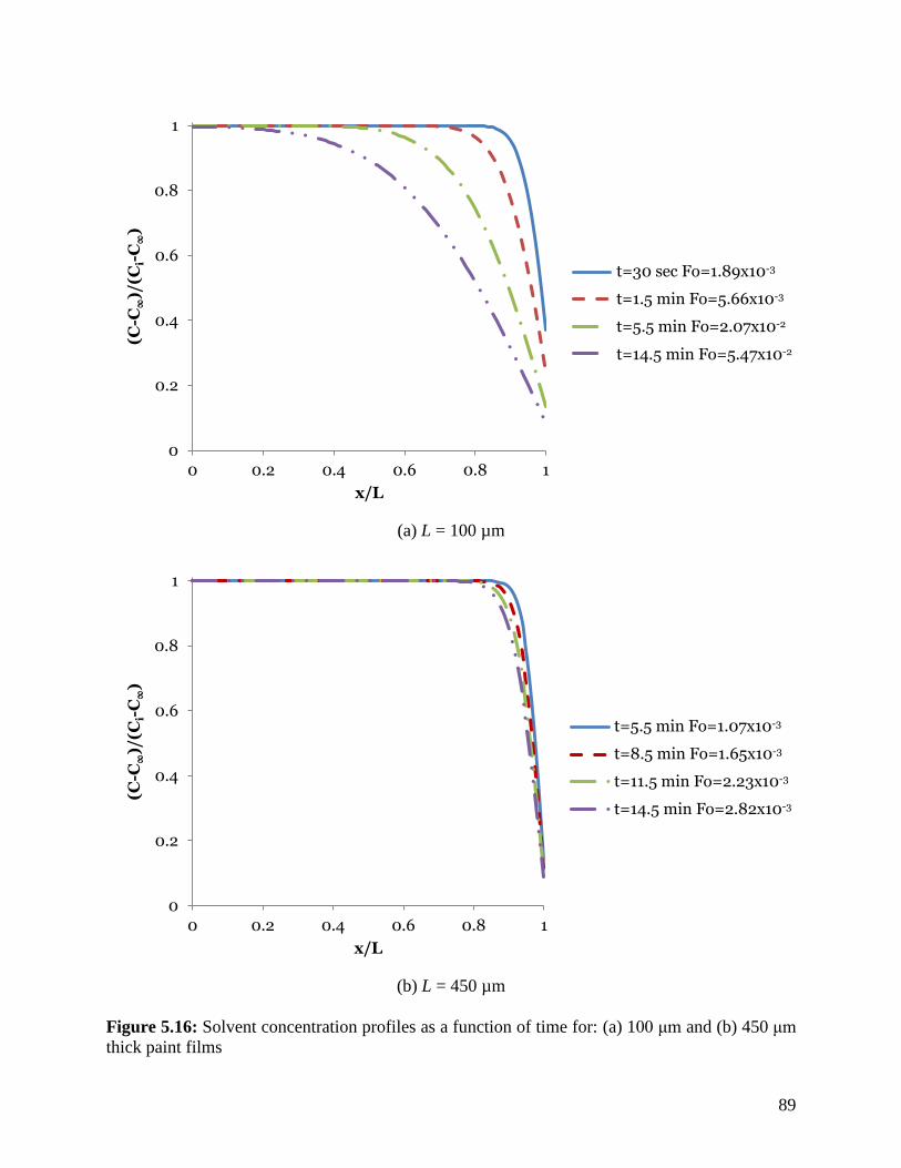
89

(a) L = 100 µm

(b) L = 450 µm

Figure 5.16: Solvent concentration profiles as a function of time for: (a) 100 μm and (b) 450 μm

thick paint films

0

0.2

0.4

0.6

0.8

1

0 0.2 0.4 0.6 0.8 1

(C-C

∞)/

(Ci-

C∞

)

x/L

t=30 sec Fo=1.89E-3

t=1.5 min Fo=5.66E-3

t=5.5 min Fo=2.07E-2

t=14.5 min Fo=5.47E-2

0

0.2

0.4

0.6

0.8

1

0 0.2 0.4 0.6 0.8 1

(C-C

∞)/

(Ci-

C∞

)

x/L

t=5.5 min Fo=1.07E-3

t=8.5 min Fo=1.65E-3

t=11.5 min Fo=2.23E-3

t=14.5 min Fo=2.82E-3

t=30 sec Fo=1.89x10-3

t=1.5 min Fo=5.66x10-3

t=5.5 min Fo=2.07x10-2

t=14.5 min Fo=5.47x10-2

t=5.5 min Fo=1.07x10-3

t=8.5 min Fo=1.65x10-3

t=11.5 min Fo=2.23x10-3

t=14.5 min Fo=2.82x10-3

90

Marangoni numbers (Ma) calculated from Equation 5.6 are shown in Figure 5.17 as a

function of time. Ma is proportional to L2, and so is larger for thicker films, which explains why

flow velocities were so much higher in the L = 450 µm film (Fig. 5.6). At t = 0, when the

concentration of solvent in the paint film is uniform everywhere, Ma=0. For our film

thicknesses, the concentration gradient increases continuously over the observation period and

never decreases and therefore Ma increases continuously as well.

Figure 5.17: Marangoni number as a function of time for paint films of varying thickness

Although Ma continued to increase throughout the 900 s observation period for all films, the

bubble velocity began to decrease much earlier: the 100 µm film stopped moving after 100 s and

the 150 µm film after approximately 300 s (Fig. 5.6). These correspond to the times that most

0

5

10

15

20

25

30

0 200 400 600 800 1000

Ma

ra

ng

on

i N

um

be

r (

x 1

05)

Time (seconds)

100 um

150 um

260 um

450 um

91

bubbles escaped from these paint films (Fig. 5.4). The decrease in velocity can be attributed to

the increase in paint viscosity due to evaporation of the solvent. As solvent is depleted in the top

layer of the paint film the viscosity increases very sharply (Fig. 5.1a), and reduces the flow

velocity in the paint film. The high viscosity surface layer also prevents bubbles from breaking

through the surface of the paint and escaping (Figs. 5.7 and 5.8). The solvent loss was greatest in

the thinner films (Fig. 5.14), reducing their velocity the most. In contrast, for the 450 µm film,

the increase in viscosity was less significant and the paint film remained mobile allowing

bubbles to escape during the entire 900 s observation time (Fig. 5.4). As bubbles collided with

each other and coalesced the average bubble diameter also increased (Fig. 5.5) in the L = 450 µm

paint film.

5.4 CONCLUSION

The time taken for bubbles in sprayed paint films with thickness 100 to 450 µm to escape

varied from 100 to 900 s, increasing with the thickness of the layer. The Sauter mean diameter of

bubbles in films less than 300 µm thick decreased as a function of time, showing that larger

bubbles escaped faster than small bubbles. The mean diameter of bubbles in a thick paint film

(450 µm) increased with time as bubbles coalesced with each other. Bubbles were observed to be

carried along with the paint as it moved due to surface tension gradient induced flows, reaching

velocities of up to 30 µm/s. Bubble velocity increased with paint film thickness.

Buoyancy forces were not the sole reason for bubble departure from the paint film: they were

observed to leave both upward and downwards facing surfaces. Bubbles in a layer of 87 wt%

92

glycerin in water mixture, which had no volatile component, did not escape and the liquid did not

move. Concentration gradients caused by solvent evaporation in a paint film create surface

tension variations that drive flows. An analytical one-dimensional model of solvent diffusion

was used to calculate concentration variations in the paint film and the Marangoni number.

In all paint layers, Ma continuously increased since concentration gradients also continuously

increased over the observation period. In thin films, the time scale for movement of bubbles and

a rapid decrease in their number varied from 100 to 300 s. The decrease in film and bubble

velocity after this time was attributed to the substantial increase in paint viscosity as the solvent

evaporated. In the thick paint layer (450 µm), the increase in viscosity was smaller and the paint

flow was stronger leading to bubbles moving and escaping throughout the entire 15 minutes.

93

CHAPTER 6

SUMMARY, CONCLUSIONS AND FUTURE WORK

6.1 SUMMARY & CONCLUSIONS

The objective of this thesis was to investigate the causes of paint defects observed in the

automotive industry focusing on uniform film formation and bubble structure in such films. First

droplet deposition and its influencing parameters were studied before sprays were analyzed.

Droplet generator systems capable of creating two-dimensional paint films as well as liquid

films through deposition and coalescence of individual droplets were designed. Mono-disperse

spray capable of generating multiple equal-sized droplets was built. A versatile setup for

photographing spray experiments from below and varying different experimental parameters

such as nozzle to substrate spacing with ease was constructed.

Individual droplet deposition and coalescence experiments showed the effect of droplet

displacement on the continuity, shape and thickness of liquid films. When overlapping droplets

are deposited surface tension forces pulled impacting droplets towards those already on the

surface, a phenomena known as drawback. Droplets deposited close to one another (large

overlap) coalesced to form a circular film. Whereas, droplets placed at a larger distance and

therefore less interaction, formed square sheets. As overlap was further decreased lines and

sheets became discontinuous. A simple model was developed to predict the conditions under

which rupture occurred. The lowest droplet overlap ratio (defined as droplet overlap distance

divided by droplet spread diameter) at which a continuous liquid film could be formed was

λ = 0.293. At large overlap ratios (λ>0.6) droplets deposited in a square array formed a circular

94

film. The minimum thickness of a continuous film formed by coalescence of droplets was shown

to vary from 5% to 70% of the initial droplet diameter while increasing impact Weber and

Reynolds number reduced the film thickness.

Mono-disperse spray experiments utilizing a pneumatic droplet generator confirmed the

presence of drawback in such sprays and as a result liquid agglomeration on the surface.

Measurements from photographs generated a correlation for the growth of the wetted area with

time. The overlap ratio between the droplets during film formation was calculated for each time

step using the wetted surface area measurement and the number of droplets deposited.

Continuous liquid films formed once the overlap ratio surpassed the critical value of λ=0.293.

The minimum number of droplets needed to cover a known area with a continuous liquid film as

well as the largest area that can be covered by a continuous liquid film given a volume of fluid

was predicted.

Local liquid pockets were also seen in full spray experiments. Droplet coalescence and

drawback led to the creation of liquid islands that grew over time as smaller impacting droplets

got pulled into the larger masses on the substrate. Pressure difference between the droplets drove

liquid motion. The liquid bridge connecting two coalescing droplets has negative curvature and

hence negative pressure in it, while both droplet surfaces have positive curvature and therefore a

positive pressure. This pressure difference creates a flow in both droplets from the peripheries

towards the center making them coalesce. The effect of volume ratio as well as overlap ratio on

the coalescence of droplets was studied. A greater disparity in the volume of the droplets causes

a larger curvature difference and therefore pressure variation. Also, the larger the center-to-

center distance between the two drops, the greater the pressure difference driving the two drops

95

together. It was concluded that spraying small droplets with large overlap was the best option to

ensure a uniform thin film.

Bubble entrapment and escape from sprayed films was examined by spraying a model paint

consisting of resin dissolved in butanol onto horizontal glass substrates to form films varying

from 100 µm to 450 µm in thickness. The substrates were photographed at 5 s intervals and

image analysis software used to measure the number, diameter and velocity of air bubbles

trapped in the paint layer. Painted substrates were weighed to determine the rate of solvent

evaporation. Bubbles escaped from the paint in 100 to 900 s, the time increasing with paint

thickness. The Sauter mean diameter of bubbles in films less than 300 µm in thickness decreased

with time because larger bubbles escaped faster than small bubbles, while the mean diameter of

bubbles in a 450 µm thick layer increased due to bubble coalescence. Bubble velocities due to

movement of the liquid increased with paint thickness and reached 30 µm/s. Bubbles escaped

from both upward and downwards facing surfaces. Concentration gradients due to solvent

evaporation in a paint film create surface tension variations that drive Marangoni flows, which

bring bubbles to the paint surface. An analytical one-dimensional model of solvent diffusion was

used to calculate solvent concentration variations in the paint film and the Marangoni number.

96

6.2 CONTRIBUTIONS

Important contributions towards the understanding the formation and bubble structure of

automotive paint films was made in this thesis as listed below:

Predicting the shape, thickness and continuity of liquid films for a given droplet size

and spacing.

Extending the findings for individual droplet coalescence to sprays.

Determining the spray droplet size and overlap criteria for achieving uniform thin

film.

Establishing bubble escape mechanism from paint films along with estimation of

forces and flows involved.

6.3 FUTURE WORK

Several recommendations on furthering the work done in this research are:

The spray investigation can be carried out with different nozzle to substrate spacing

as well as various liquids and substrates. Changing these parameters will respectively

showcase the effect of overlap ratio and contact angle on the film formation.

The spray investigation can be extended to calculate the overlap ratio between the

impacting droplets and determine whether the critical overlap value λ=0.293 for

continuous liquid films holds.

97

REFERENCES

[1] R.G. Nallicheri, “Automotive painting: an economic and strategic analysis”, M.S. thesis,

Sloan School of Management, Massachusetts Institute of Technology, Cambridge, MA, USA,

1994.

[2] C.A. Geffen and S. Rothenberg, “Suppliers and environmental innovation: The automotive

paint process”, International Journal of Operations and Production Management, Vol. 20, pp.

166-186, 2000.

[3] J. Domnick, A. Scheibe and Q. Ye, “The simulation of the electrostatic spray painting

process with high-speed rotary bell automizers. Part I: Direct Charging”, Particle & Particle

Systems Characterization, Vol. 22, pp. 141-150, 2005.

[4] D.C. Conner, P.N. Atkar, A.A. Rizzi and H. Choset, “Development of deposition models for

paint application on surfaces embedded in IR3 for use in automated path planning”, Proceedings

IEEE/RSJ International Conference on Intelligent Robots and Systems, Vol. 2, pp. 1844-9, 2002.

[5] H.T. Charles Fan and H. Kuo, General Motors Research and Development, Personal

Communication

[6] R. Talbert, Paint Technology Handbook, Boca Raton, FL: CRC Press, 2008.

[7] A. Goldschmidt and H.J. Streitberger, BASF Handbook on Basics of Coating Technology,

Hannover, Germany: BASF Coatings AG, 2003.

98

[8] I. Lewin, “Product, paint and curing method: the essential components of an integrated

coating system”, Pigment & Resin Technology, Vol. 28, pp. 158-161, 1999.

[9] R.C. Leach, “Curing with infrared and combination ovens”, Industrial Paint and Powder,

Vol. 80, pp. 16-20, 2004.

[10] BASF, “Paint Defects Advice”, Online Resource, Accessed August 3, 2011:

http://www.carpaintdepot.com/docs/basf/Paint_Defects.pdf

[11] HMG Paints Ltd, “HMG Troubleshooting”, Online Resource, Accessed August 3, 2011:

http://www.hmgpaint.com/troubleshooting/

[12] W.S. Overdiep, “The levelling of paints”, Progress in Organic Coatings, Vol. 14, pp.159-

175, 1986.

[13] R. Radfar, J. Jassbi, F. Ghoreishi, S. Khanmohammadi and M. Alborzi, “Proactive quality

paint thickness control using ANFIS”, 2010 IEEE International Conference on Systems, Man

and Cybernetics (SMC 2010), Istanbul, Turkey, 2010, pp. 5-10.

[14] S.D. Howison, J.A. Moriarty, J.R. Ockendon, E.L. Terrill and S.K. Wilson, “A

mathematical model for drying paint layers”, Journal of Engineering Mathematics, Vol. 32, pp.

377-394, 1997.

[15] B.-J. de Gans, P. C. Duineveld and U. S. Schubert, “Inkjet printing of polymers: state of the

art and future developments”, Advanced Materials, Vol. 16, pp. 203-213, 2004.

99

[16] M. Fang, S. Chandra and C.B. Park, “Building three-dimensional objects by deposition of

molten metal droplets”, Rapid Prototyping Journal, Vol. 14, pp.44-52, 2008.

[17] T. Boland, T. Xu, B. Damon and X. Cui, “Application of inkjet printing to tissue

engineering”, Biotechnology Journal, Vol. 1, pp. 910-917, 2006.

[18] P.C. Duineveld, “The stability of ink-jet printed lines of liquid with zero receding contact

angle on a homogeneous substrate”, Journal of Fluid Mechanics, Vol. 477, pp. 175-200, 2003.

[19] C. Andrieu, D. Beysens, V.S. Nikolayev and Y. Pomeau, “Coalescence of sessile drops”,

Journal of Fluid Mechanics, vol. 453, pp. 427-438, 2002.

[20] I.V. Roisman, B. Prunet-Foch, C. Tropea and M. Vignes-Adler, “Multiple drop impact onto

a dry solid substrate”, Journal of Colloid and Interface Science, Vol. 256, pp. 396-410, 2002.

[21] S.T. Thoroddsen, K. Takehara and T.G. Etoh, “The coalescence speed of a pendent and a

sessile drop”, Journal of Fluid Mechanics, Vol. 527, pp. 85-114, 2005.

[22] R. Li, N. Ashgriz, S. Chandra, J.R. Andrews and J. Williams, “Drawback during deposition

of overlapping molten wax droplets”, Journal of Manufacturing Science and Engineering, Vol.

130, pp. 041011-1–10, 2008.

[23] R. Narhe, D. Beysens and V.S. Nikolayev, “Contact line dynamics in drop coalescence and

spreading”, Langmuir, Vol. 20, pp. 1213-1221, 2004.

[24] R. Li, N. Ashgriz, S. Chandra, J. Andrews and S. Drappel, “Coalesence of two droplets

impacting a solid surface”, Experiments in Fluids, Vol. 48, pp. 1025-1035, 2010.

100

[25] F. Goa and A.A. Sonin, “Precise deposition of molten microdrops: the physics of

microfabrication”, Proceedings of the Royal Society of London, Series A: Mathematical,

Physical and Engineering Sciences, Vol. 444, pp. 533-554, 1994.

[26] J.R. Castrejon-Pita, E.S. Betton, K.J. Kubiak, M.C.T. Wilson and I.M. Hutchings, “The

dynamics of the impact and coalescence of droplets on a solid surface”, Biomicrofluidics, Vol. 5,

pp. 014112-1–20, 2011.

[27] P.J. Graham, M.M. Farhangi and A. Dolatabadi, “Dynamics of droplet coalescence in

response to increasing hydrophobicity”, Physics of Fluids, Vol. 24, pp. 112105-1–20, 2012.

[28] L. A. Kornum and H. K. Raaschou Nielsen, “Surface defects in drying paint films”,

Progress in Organic Coatings, Vol. 8, pp. 275-324, 1980.

[29] H. J. Streitberger and K. F. Dössel, Automotive Paints and Coatings, Weinheim, Germany:

Wiley-VCH Verlag GmbH & Co., 2008.

[30] J. Domnick, D. Gruseck, K. Pulli, A. Scheibe, Q. Ye and F. Brinckmann, “Investigations of

the drying process of a water based paint film for automotive applications”, Chemical

Engineering and Processing, Vol. 50, pp. 495–502, 2011.

[31] S. Chandra and C.T. Avedisian, "On the collision of a droplet with a solid surface",

Proceedings of the Royal Society of London, Series A: Mathematical, Physical and Engineering

Sciences, Vol. 432, pp. 13-41, 1991.

[32] V. Mehdi-Nejad, J. Mostaghimi and S. Chandra, "Air bubble entrapment under an

impacting droplet", Physics of Fluids, Vol. 15, pp. 173-183, 2003.

101

[33] J.S. Lee, B.M. Weon, J.H. Je and K. Fezzaa, "How does an air film evolve into a bubble

during droplet impact?", Physical Review Letters, Vol. 109, pp. 204501-1-5, 2012.

[34] S.T. Thoroddsen, K. Takehara, And T.G. Etoh, "Bubble entrapment through topological

change", Physics of Fluids, Vol. 22, pp. 051701-1-4, 2010.

[35] M.M. Driscoll, C.S. Stevens and S.R. Nagel, "Thin film formation during splashing of

viscous liquids", Physical Review E, Vol. 82, pp. 036302-1-7, 2010.

[36] D.B. van Dam and C. Le Clerc, "Experimental study of the impact of an ink-jet printed

droplet on a solid substrate", Physics of Fluids, Vol. 16, pp. 3403-3414, 2004.

[37] S.T. Thoroddsen, T.G. Etoh, K. Takehara, N. Ootsuka and Y. Hatsuki, "The air bubble

entrapped under a drop impacting on a solid surface", Journal of Fluid Mechanics, Vol. 545, pp.

203-212, 2005.

[38] J. Eggers, "Air entrainment through free-surface cusps", Physical Review Letters, Vol. 86,

pp. 4290-4293, 2001.

[39] P. A. Elmore, G.L. Chahine, and H.N. Oguz, "Cavity and flow measurements of

reproducible bubble entrainment following drop impacts", Experiments in Fluids, Vol. 31, pp.

664-673, 2001.

[40] S.T. Thoroddsen, T.G. Etoh and K. Takehara, "Air entrapment under an impacting drop",

Journal of Fluid Mechanics, Vol. 478, pp. 125-134, 2003.

102

[41] Q. Deng, A.V. Anilkumar, and T.G. Wang, "The role of viscosity and surface tension in

bubble entrapment during drop impact onto a deep liquid pool", Journal of Fluid Mechanics,

Vol. 578, pp. 119-138, 2007.

[42] D.L. Keij, K.G. Winkels, H. Castelijins, M. Riepen and J.H. Snoeijer, "Bubble formation

during the collision of a sessile drop with a meniscus”, Physics of Fluids, Vol. 25, pp. 082005-1-

13, 2013.

[43] M. Kadoura, “The formation and drying of thin paint films sprayed on a solid surface”,

M.A.Sc thesis, Department of Mechanical & Industrial Engineering, University of Toronto,

Toronto, ON, 2011.

[44] The Dow Chemical Company, OPTIM Synthetic Glycerine – Physical Properties [Online].

Available: http://www.dow.com/optim/optim-advantage/physical-properties.htm

[45] D. Khossravi and K.A. Connors, “Solvent effects on chemical processes. 3. Surface tension

of binary aqueous organic solvents”, Journal of Solution Chemistry, Vol. 22, pp. 321-330, 1993.

[46] R. Bhola and S. Chandra, “Parameters controlling solidification of molten wax droplets

falling on a solid surface”, Journal of Materials Science, Vol. 34, pp. 4883-4894, 1999.

[47] R. Li, “Droplet deposition in solid ink printing”, Ph.D. dissertation, Department of

Mechanical & Industrial Engineering, University of Toronto, Toronto, ON, 2008.

[48] M. Pasandideh-Fard, Y.M. Qiao, S. Chandra and J. Mostaghimi, “Capillary effects during

droplet impact on a solid surface”, Physics of Fluids, Vol. 8, pp.650-659, 1996.

103

[49] P. Meakin, “Droplet deposition growth and coalescence”, Reports on Progress in Physics,

Vol. 55, pp. 157-240, 1992.

[50] E. Specht. (2015, February 21). The best known packings of equal circles in a square

[Online]. Available: http://hydra.nat.uni-magdeburg.de/packing/csq/csq.html#overview

[51] J. Esmaeelpanah, A. Dalili, S. Chandra and J. Mostaghimi, "Coalescence and drawback of

unequal sized droplets deposited on a surface", Proceedings of the Canadian Society for

Mechanical Engineering International Congress, Toronto, ON, Canada, 2014.

[52] H. Javaheri, “Automotive Paint Properties”, M.Eng thesis, Department of Chemical

Engineering, University of Toronto, Toronto, ON, 2013.

[53] Dow. (2014, March 3). Butanol Technical Data Sheet [Online]. Available:

http://msdssearch.dow.com/PublishedLiteratureDOWCOM/dh_08ac/0901b803808ac9ed.pdf?file

path=oxysolvents/pdfs/noreg/327-00014.pdf&fromPage=GetDoc

[54] Q. Tseng. (2014, May 13). PIV (Particle Image Velocimetry)---ImageJ plugin [Online].

Available: https://sites.google.com/site/qingzongtseng/piv

[55] R. Clift, J. R. Grace and M. E. Weber, Bubbles, Drops and Particles, New York, NY:

Academic Press, 1978.

[56] C. Crowe, M. Sommerfeld and Y. Tsuji, Multiphase Flows with Droplets and Particles,

Boca Raton, FL: CRC Press, 1998.

104

[57] P.-S. Hahn, J.-D. Chen and J. C. Slattery, “Effects of London-van der Waals forces on the

thinning and rupture of a dimpled liquid film as a small drop or bubble approaches a fluid-fluid

interface”, AIChE Journal, Vol. 31, pp. 2026-2038, 1985.

[58] T. Sanada, M. Watanabe and T. Fukano, “Effects of viscosity on coalescence of a bubble

upon impact”, Chemical Engineering Science, Vol. 60, pp. 5372-5384, 2005.

[59] H. Kočárková, F. Rouyer and F. Pigeonneau, “Film drainage of viscous liquid on top of bare

bubble Influence of the Bond number”, Physics of Fluids, Vol. 25, pp.022105-1-14, 2013.

[60] T. Köllner, K. Schwarzenberger, K. Eckert and T. Boeck, “Multiscale structures in solutal

Marangoni convection: Three-dimensional simulations and supporting experiments”, Physics of

Fluids, Vol. 25, pp.092109-1-31, 2013.

[61] N. Saranjam, S. Chandra, J. Mostaghimi, H. Fan and J. Simmer, “Surface tension-driven

flows within drying paint films”, Proceedings of the 15th International Heat Transfer

Conference, Kyoto, Japan, 2014, IHTC15-8582.

[62] J. Crank, The Mathematics of Diffusion, Oxford, UK: Clarendon Press, 1975.

[63] L. Ion and J. M. Vergnaud, “Process of drying a polymeric film by diffusion – evaporation

and shrinkage. Determination of the concentration-dependent diffusivity”, Polymer Testing, Vol.

14, pp. 479-487, 1995.

[64] J. M. Vergnaud, Drying of Polymeric and Solid Materials: Modelling and Industrial

Applications, New York, NY: Springer-Verlag, 1992.

105

[65] B. Doda. (2015, July 22). PDPA [Online]. Available:

http://velocimetry.net/pdpa_principles.htm

[66] TSI (2015, July 22). PDPA Systems [Online]. Available:

http://www.tsi.com/pdpa-systems/

106

APPENDIX A

ENGINEERING DRAWING OF MECHANICAL PARTS

Engineering drawings of major components of the experimental setups are provided in this

appendix. All units are in millimeters except for Figure A.4 which was requested in inches.

Figure A.1: Opal diffusing glass holder

Figure A.2: Mono-disperse spray nozzle body

Figure A.3: Mono-disperse spray nozzle plate

Figure A.4: Spray fixture substrate holder

Figure A.5: PDPA spray mounting plate

107

Figure A.1: Opal diffusing glass holder

108

Figure A.2: Mono-disperse spray nozzle body

109

Figure A.3: Mono-disperse spray nozzle plate

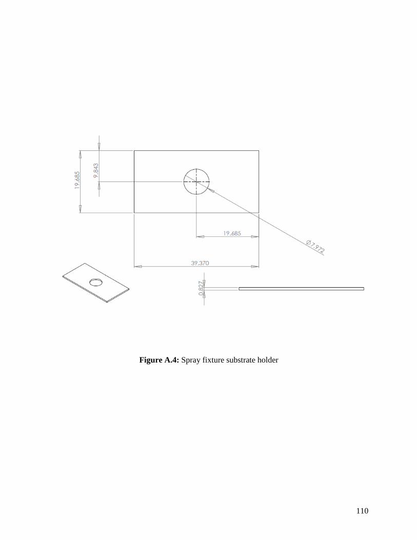
110

Figure A.4: Spray fixture substrate holder

111

Figure A.5: PDPA spray mounting plate

112

APPENDIX B

TRANSLATION MOTION SYSTEM AND COMPUTER

SOFTWARE

The translation motion system consists of an x-y motion stage (XYR-1010, Danaher

Precision Motion, Chicago, IL, USA) with 200 mm x 200 mm (8 in. x 8 in.) travel. The motion

of the individual axes of the stage is independent and can be coordinated in order to implement

any complex motion under the control of a 4-axis motion controller board (DMC-1840, Galil

Motion Control, Inc., Rocklin, CA). The controller board is connected to a junction box which

directs the commands from the controller board to an amplifier used to drive the motors on the

stage. The junction box also receives encoder readings from the motors which allow the user to

exactly know the position of each axis of the stage.

Computer software developed by Fang [16] was used to control the system. The software

provides a program editor window where the motion program to control the movement of the x-y

stage can be entered. The program is based on the geometrical characteristics of the object that is

to be created. The Galil program syntax consists of designated double-lettered commands

understood by the Galil motion control board. Furthermore, a section of the software is dedicated

to process parameters involved in producing and dispensing droplets, such as deposition rate and

stage speed, thus synchronizing stage motion and droplet delivery. Finally, the status of the

motion stage, such as the speed of individual axes and current coordinates of the stage are

tracked and relayed to the user.

113

Figure B.1: Software interface developed for motion stage control and droplet deposition [16]

Motion program samples written to create liquid lines and two-dimensional liquid films are

presented below and comments on key control commands are provided as well. For each desired

overlap ratio, the center-to-center distance between the droplets would be calculated based on the

known droplet spread diameter. Since it was known that each count of the x-y motion stage had a

speed of 0.5 µm/s, the appropriate stage speed count would be included in the program.

Detailed instructions on how to program the motion stage can be found in the user manual and

program guide provided by Galil Motion Inc.

114

a) Motion program for fabrication of 12x12 two-dimensional 87 wt% glycerin liquid film with

L=2.17 mm in Chapter 2

#LINE SHEET //Program label

COUNT=1 //Initialize variables

BILINES= 6

DCX=100000 //Specify deceleration of both x and y axis

DCY=100000

SP 4348, 4348 //Specify speed of both x and y axis

#LOOP //Start a loop to implement droplet deposition on multiple lines

PRY=52176 //Move 52176 steps in positive y direction

BGY //Begin y-axis motion

CB0 //Set output0 to high which is used to initiate droplet deposition

AMY //After y-axis motion

SB0 //Set output0 to low which is used to suspend droplet deposition

PRX=4348 //Move 4348 steps in positive x direction

BGX

AMX

PRY=-52176 //Move 52176 steps in negative y direction

BGY

CB0

AMY

SB0

PRX=4348

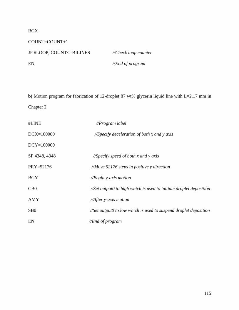
115

BGX

COUNT=COUNT+1

JP #LOOP, COUNT<=BILINES //Check loop counter

EN //End of program

b) Motion program for fabrication of 12-droplet 87 wt% glycerin liquid line with L=2.17 mm in

Chapter 2

#LINE //Program label

DCX=100000 //Specify deceleration of both x and y axis

DCY=100000

SP 4348, 4348 //Specify speed of both x and y axis

PRY=52176 //Move 52176 steps in positive y direction

BGY //Begin y-axis motion

CB0 //Set output0 to high which is used to initiate droplet deposition

AMY //After y-axis motion

SB0 //Set output0 to low which is used to suspend droplet deposition

EN //End of program

116

APPENDIX C

PHASE DOPPLER PARTICLE ANALYZER (PDPA)

Phase Doppler Particle Analyzers (PDPA) can quantify the size and velocity of spray

droplets at the same time. The device combines laser-based optical transmitter, an optical

receiver, an electronic signal processor and software to obtain and analyze the data [65].

As mentioned by [66], Phase Doppler method is based on light scattering interferometry. The

intersection of the two laser beams defines a non-intrusive sample volume location. When a

droplet travels through the sample volume, light from the probes is scattered into a multi-detector

receiving probe strategically positioned at an off-axis collection angle. The phase shift between

the signals from the different detectors is proportional to the size of the droplets.

Figure C.1: TSI PDPA system used for measuring spray droplet size

Laser Transmitter

Optical Receiver

Spray Nozzle

Signal Processing & Photodetector

Modules

Laser

117

The TSI FlowSizer data acquisition and analysis software provides a comprehensive

interface for setting the parameters of the different equipment in the system and presents the

gathered data in user-defined graphics and statistics reports. Some of the diameter measurement

fields included in the Run Statistics report is D10, D20, D30, D32, D43 and Size Valid Count.

Figure C.2 showcases some of the windows displayed by FlowSizer pertaining to droplet size

distribution and measurements. More information on the TSI PDPA system and the FlowSizer

software can be found in Phase Doppler Particle Analyzer (PDPA) operations manual provided

by TSI.

Figure C.2: TSI FlowSizer software Interface [66]