Embed Size (px)
Citation preview
A Review on Liquid Spray Models for Diesel Engine
Computational Analysis
by Luis Bravo and Chol-Bum Kweon
ARL-TR-6932 May 2014 Approved for public release; distribution is unlimited.
NOTICES
Disclaimers The findings in this report are not to be construed as an official Department of the Army position unless so designated by other authorized documents. Citation of manufacturer’s or trade names does not constitute an official endorsement or approval of the use thereof. Destroy this report when it is no longer needed. Do not return it to the originator.
Army Research Laboratory Aberdeen Proving Ground, MD 21005-5069
ARL-TR-6932 May 2014
A Review on Liquid Spray Models for Diesel Engine Computational Analysis
Luis Bravo and Chol-Bum Kweon Vehicle Technology Directorate, ARL
Approved for public release; distribution is unlimited.
ii
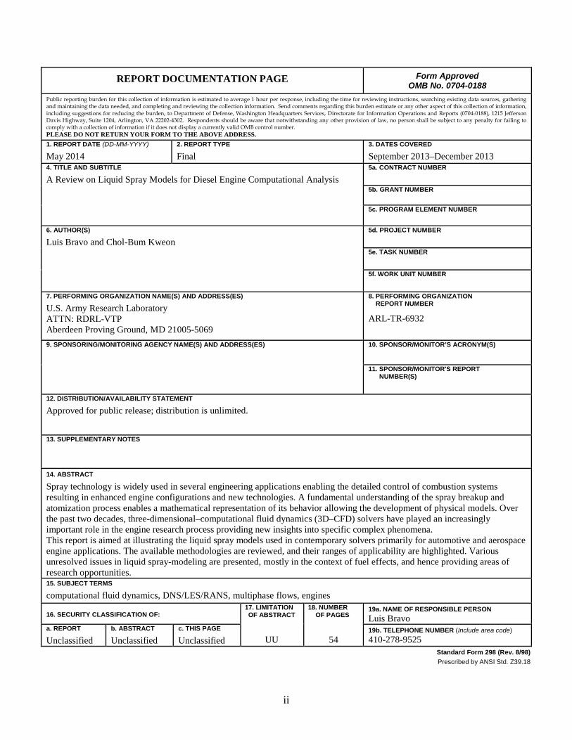
REPORT DOCUMENTATION PAGE Form Approved OMB No. 0704-0188
Public reporting burden for this collection of information is estimated to average 1 hour per response, including the time for reviewing instructions, searching existing data sources, gathering and maintaining the data needed, and completing and reviewing the collection information. Send comments regarding this burden estimate or any other aspect of this collection of information, including suggestions for reducing the burden, to Department of Defense, Washington Headquarters Services, Directorate for Information Operations and Reports (0704-0188), 1215 Jefferson Davis Highway, Suite 1204, Arlington, VA 22202-4302. Respondents should be aware that notwithstanding any other provision of law, no person shall be subject to any penalty for failing to comply with a collection of information if it does not display a currently valid OMB control number. PLEASE DO NOT RETURN YOUR FORM TO THE ABOVE ADDRESS. 1. REPORT DATE (DD-MM-YYYY)
May 2014 2. REPORT TYPE
Final 3. DATES COVERED
September 2013–December 2013 4. TITLE AND SUBTITLE
A Review on Liquid Spray Models for Diesel Engine Computational Analysis 5a. CONTRACT NUMBER
5b. GRANT NUMBER
5c. PROGRAM ELEMENT NUMBER
6. AUTHOR(S)
Luis Bravo and Chol-Bum Kweon 5d. PROJECT NUMBER
5e. TASK NUMBER
5f. WORK UNIT NUMBER
7. PERFORMING ORGANIZATION NAME(S) AND ADDRESS(ES)
U.S. Army Research Laboratory ATTN: RDRL-VTP Aberdeen Proving Ground, MD 21005-5069
8. PERFORMING ORGANIZATION REPORT NUMBER
ARL-TR-6932
9. SPONSORING/MONITORING AGENCY NAME(S) AND ADDRESS(ES)
10. SPONSOR/MONITOR’S ACRONYM(S) 11. SPONSOR/MONITOR'S REPORT NUMBER(S)
12. DISTRIBUTION/AVAILABILITY STATEMENT
Approved for public release; distribution is unlimited.
13. SUPPLEMENTARY NOTES
14. ABSTRACT
Spray technology is widely used in several engineering applications enabling the detailed control of combustion systems resulting in enhanced engine configurations and new technologies. A fundamental understanding of the spray breakup and atomization process enables a mathematical representation of its behavior allowing the development of physical models. Over the past two decades, three-dimensional–computational fluid dynamics (3D–CFD) solvers have played an increasingly important role in the engine research process providing new insights into specific complex phenomena. This report is aimed at illustrating the liquid spray models used in contemporary solvers primarily for automotive and aerospace engine applications. The available methodologies are reviewed, and their ranges of applicability are highlighted. Various unresolved issues in liquid spray-modeling are presented, mostly in the context of fuel effects, and hence providing areas of research opportunities. 15. SUBJECT TERMS
computational fluid dynamics, DNS/LES/RANS, multiphase flows, engines
16. SECURITY CLASSIFICATION OF: 17. LIMITATION OF ABSTRACT
UU
18. NUMBER OF PAGES
54
19a. NAME OF RESPONSIBLE PERSON Luis Bravo
a. REPORT
Unclassified b. ABSTRACT
Unclassified c. THIS PAGE
Unclassified 19b. TELEPHONE NUMBER (Include area code) 410-278-9525
Standard Form 298 (Rev. 8/98) Prescribed by ANSI Std. Z39.18
iii
Contents
List of Figures v
List of Tables vi
1. Summary 1
2. Introduction 2
3. Physical Description 5
3.1 Primary Atomization .......................................................................................................7
3.2 Secondary Atomization ...................................................................................................9
4. Spray Modeling 11
4.1 The Spray Equation: A Statistical Description ..............................................................12 4.1.1 Droplet Acceleration .........................................................................................12 4.1.2 Drop Radius .......................................................................................................13 4.1.3 Drop Temperature .............................................................................................13 4.1.4 Drop Deformation .............................................................................................14 4.1.5 Drop Collisions ..................................................................................................14
4.2 Review of Liquid Spray Breakup Models .....................................................................15 4.2.1 KH Breakup Model ...........................................................................................15 4.2.2 Blob Injection Model .........................................................................................19 4.2.3 Linearized Instability Sheet Atomization (LISA) Breakup Model ...................21 4.2.4 Taylor Analogy Breakup (TAB) and E-TAB Breakup Model ..........................24 4.2.5 RT/Hybrid KH-RT/Modified KH-RT Breakup Model .....................................27 4.2.6 KH-ACT (Aerodynamics, Cavitation, and Turbulence) Breakup Model .........29
5. Summary and Outlook 33
5.1 Summary .......................................................................................................................34
5.2 Unresolved Issues and Directions .................................................................................36
6. References 38
iv
List of Symbols, Abbreviations, and Acronyms 43
Distribution List 45
v
List of Figures
Figure 1. Various stages of high-pressure diesel spray breakup. .....................................................6
Figure 2. Disintegration of circular water jet in pressure atomization (d=1.5mm). ........................8
Figure 3. Primary fragmentation modes of a liquid jet in pressurized atomization. ........................8
Figure 4. Jet-stability curve showing the breakup length modes and dependence with velocity. ......................................................................................................................................9
Figure 5. Breakup modes in secondary droplet breakup. ...............................................................11
Figure 6. Schematic growth of surface perturbations in KH model. Notation 1 depicts the liquid phase, while 2 depicts the gas phase..............................................................................16
Figure 7. Wave growth rate vs. wave number as a function of Weber number and Ohnesorge number. ....................................................................................................................................17
Figure 8. Physical behavior of (a) wavelength and (b) growth rate of the most unstable surface wave.............................................................................................................................18
Figure 9. Illustration of the blob-injection model of Reitz et al.. ..................................................19
Figure 10. Schematic (a) sheet and spray formation with a pressure swirl injection, (b) breakup mechanism of planar liquid sheets . ...........................................................................21
Figure 11. (a) Quantitative droplet distribution from atomizer; measured and predicted (b) Spray penetration, (c) SMD with inwardly opening injectors (Conditions: 𝑃𝑖𝑛𝑗 =4.86 𝑀𝑃𝑎 , 𝑚𝑖𝑛𝑗 = 44 𝑚𝑔 , 𝑑𝑢𝑟𝑖𝑛𝑗 = 3.86 𝑚𝑠, and fuel density, 𝜌𝑓 = 0.77 𝑔/𝑐𝑚3 ) ......24
Figure 12. Drop distribution in the near field for t_inj = 1.0 ms after 100 d downstream (𝑃𝑖𝑛𝑗 = 300 𝑏𝑎𝑟). ...................................................................................................................26
Figure 13. Comparison of liquid penetration profiles with E-TAB for 3 cases at 𝑃𝑖𝑛𝑗 =300 𝑏𝑎𝑟. Top case conditions: 𝑃𝑔𝑎𝑠 = 11 𝑏𝑎𝑟 , 𝑡𝑖𝑛𝑗 = 2.5 𝑚𝑠; Middle case: 𝑃𝑔𝑎𝑠 =30 𝑏𝑎𝑟 , 𝑡𝑖𝑛𝑗 = 4.0 𝑚𝑠 ; Bottom case: 𝑃𝑔𝑎𝑠 = 50 𝑏𝑎𝑟 , 𝑡𝑖𝑛𝑗 = 5.0 𝑚𝑠 . .............................27
Figure 14. KH-RT liquid model validation (a) penetration length validation with x-ray data (b) effect of ROI on penetration rates. .....................................................................................29
Figure 15. Primary breakup model effect on nonevaporating (a) liquid penetration profiles and (b) SMD. Conditions: 𝑃𝑖𝑛𝑗 = 1100 𝑏𝑎𝑟 , 𝜌𝑓 = 865.4 𝑘𝑔/𝑚3 ,𝑑𝑖𝑛𝑗 = 169 𝜇𝑚, 𝜌∞ = 34.13, 𝑇∞ = 298 𝐾, 10%0 𝑁2. ...................................................................................32
Figure 16. Comparison between hybrid KH model and KH-ACT model for (a) liquid penetration length variations with chamber temperature and (b) vapor penetration length variations with time. Conditions for the orifice diameter, injection pressure, and fuel temperature are: 246 𝜇𝑚, 1420 𝑏𝑎𝑟, and 438 𝐾, respectively. ..............................................33
vi
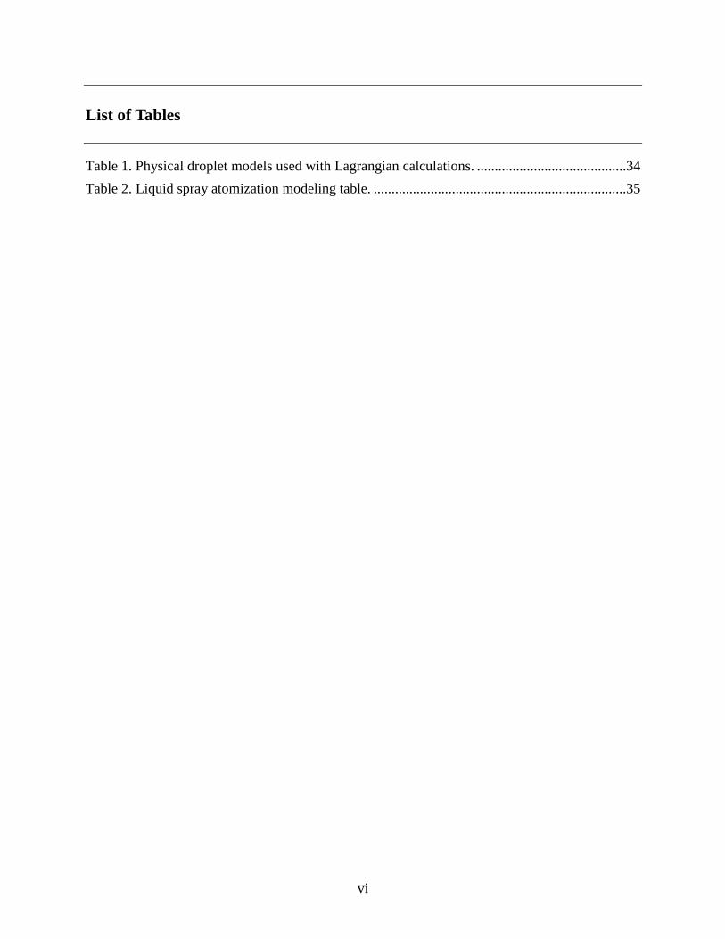
List of Tables
Table 1. Physical droplet models used with Lagrangian calculations. ..........................................34
Table 2. Liquid spray atomization modeling table. .......................................................................35
1
1. Summary
Multidimensional numerical simulation (three-dimensional–computational fluid dynamics [3D–CFD]) of the spray behavior is an integral part of engine research critical for combustion optimization and to enhance the understanding of complex in-cylinder combustion phenomena occurring in engines. Successful implementation of advanced modeling tools is strongly related to our current understanding of the physical processes involved. The importance of numerical models and simulation tools is increasing dramatically (1). Recently, it has been essential in aiding the development process of new combustion concepts providing unprecedented efficiencies (2). Such developments are critical to engine technology advancements of interest to the U.S. Army. The objective of this report is to review the leading 3D–CFD atomization models used in engine research to illustrate our current understanding, and to identify grey areas of further research.
Spray behavior can be described as a multiscale, turbulent physical process presenting several technical challenges. There is a liquid core region that is affected by the aerodynamic interaction. Once the liquid surface becomes unstable it will favor the creation of liquid ligaments that in turn will create parent “primary” droplets at first, followed by secondary “child” droplets. Droplets are reduced in size due to evaporation and combustion occurs while reduced droplets traveling downstream of the injector nozzle. Models capturing this process have had success in engineering applications, and have typically relied on empirical correlations or simplified physics. However, deeper knowledge about turbulent sprays is still needed in the community. Several reports have noted an insufficient understanding of the development of surface instabilities, ligament formation mechanisms, and droplet formation mechanism from a ligament. Nozzle effects and needle wobble conditions are also important characteristics that have not been fully resolved and strongly affect spray breakup. Improved knowledge of primary breakup will lead to better predictions of spray characteristics such as initial droplet size distribution, spray angle, and jet structure, which result in significant impacts on improving the engine combustion process.
Spray breakup models may be improved through the use of high-resolution numerical simulations. Large Eddy Simulation (LES) can provide a tradeoff between accuracy and computational cost. LES is dependent on the subgrid models to treat unresolved flow-field. Direct Numerical Simulation (DNS) is aimed at removing turbulence uncertainty and resolving all of the flow length-scales. Of key importance is resolving the droplet length scale, in addition to the flow length scale, and studying the droplet interactions with its surroundings. Computationally, DNS is still a daunting task due to its resolution requirements imposed by the droplet scale. Recently, several studies using DNS tools have made significant strides in primary atomization models using the Eularian Lagrangian Spray Atomization (ELSA) methodology and driving the
2
development of advanced models. Typically, these studies are conducted in small configurations, and are representative of efforts towards next generation atomization models for diesel sprays.
2. Introduction
The objective of this report is to review contemporary liquid spray physical models used in the computational fluid dynamics (CFD) community for engine applications. It provides a technical introduction, a presentation of the physical mechanisms, and a review/discussion of the leading models and applications.
The aims of the report are as follows:
• To provide a review of current spray modeling efforts used in the state-of-the-art engine research.
• To identify critical areas of future modeling interest that can lead to technological advancements.
• To promote engine spray research by dissemination of these findings to the scientific community.
Fundamental physical understanding of the spray atomization process is (1) critical in addressing the Army’s need to enable the advancement of efficient air and ground combat vehicles and compact fuel-to-electric power systems, and (2) essential to continue leading strategic development for portable and heavy-duty engine applications. Spray technology has a wide range of applications in engineering—such as combustion devices found in unmanned aerial systems (rotary and piston engines), aerospace propulsion systems (gas turbine engines), ground vehicle engines (piston engines), metallurgical processes (spray generated coatings) for thermal barrier, environmental barrier, substrate corrosion protection, and material strengthening (3–5). Within the context of unmanned aerial and ground vehicle engine applications, an understanding of liquid spray characteristics is critical in improving engine performance and efficiency as well as complying with strict emissions standards that require precise fuel delivery systems for optimum power and reduction of exhaust gases and particulates. Hence, detailed characterization of the spray and combustion processes is important in developing high-impact new technologies such as single-fuel optimized engines for Army engine applications.
Spray breakup is a complex phenomenon and dependent on many factors such as velocity of spray, injection pressure, geometry of nozzle, temperature of both fluids, and properties of fluid (i.e., their density, viscosity, surface tension, and vapor pressure) (6). Several detailed studies of the spray process exist in the combustion literature focusing on the atomization and breakup characteristics of fuel sprays through the use of sophisticated combustion vessels (7–10). The Engine Combustion Network (ECN) established through the efforts at Sandia National
3
Laboratories (SNL) has historically driven the experimental efforts in quantifying spray parameters with the aim of providing a high-fidelity consolidated database at diesel and gasoline engine relevant conditions. Some of the ECN affiliates that have conducted spray characterization in vessels include: SNL, French Petroleum Institute (IFPEN), Universidad Politecnica de Valencia (CMT-Motores Termicos), Caterpillar, Eindhoven University of Technology (TU/e), Michigan Technological University (MTU), and General Motors. Most recently, the U.S. Army Research Laboratory (ARL) is expanding its involvement in the ECN network. Measurements are typically conducted at well controlled high temperature and pressure conditions through the use of two distinct types of combustion vessels: Constant-Pressure Flow (CPF) and Constant-Volume Preburn (CVP) chambers. An excellent review has been published focusing on the comparison between the operations and control of boundary conditions for both types of combustion vessels (CPF and CVP) while studying a well reported case denoted as Spray A (11). Spray A uses a single component diesel surrogate fuel (n-dodecane), a single hole injector (common rail, 1500-bar fuel pressure, 363-K fuel temperature), representing a diesel engine combustion condition (900 K, 60 bar) that use a moderate rate of exhaust-gas recirculation (EGR). Using a CVP chamber, Siebers et al. (12) reported the spray liquid penetration length at near Spray A conditions and studied the spray behavior when subject to changes in operating conditions such as decreasing injector orifice diameter, injection pressure, ambient gas density or temperature, and fuel volatility. It was established that liquid length decreases linearly with injector diameter, temperature or density, increases with fuel volatility or temperature, and that it is independent of injection pressure. Extending this work, Weber et al. (13) has used a CPF type vessel at diesel conditions, together with computational methods (CFD and microgenetic algorithms), to provide optimization strategies for spray penetration and mixture formation at diesel condition (50 bar and 800 K). Similar research efforts led by Kweon (3) have been performed at the ARL for diesel and JP-8 fuels to characterize the effects of injector configuration and fuel composition on the spray parameters using a CPF vessel and optical diagnostics such as Mie scattering, Shadowgraph, and Schlieren images.
Access to spray measurements plays a key role in the development of physics-based models to be integrated into robust 3D–CFD solvers. Multidimensional CFD solvers will utilize experimental data by carrying out model-validation studies and quantifying the simulation error; hence the solver strictly relies on the fidelity of the measurement in addition to its own numerical errors. A validation study will reveal the suitability of modeling assumptions (physical models), stability of the spatio-temporal numerical technique (numerical methods), and calibration of model parameters (turbulence, breakup, combustion constants) that is required to carefully benchmark a simulation. Hence, validated modeling of spray and combustion processes enables several attributes that make its use in engine development of paramount importance; for example, its suitability in conducting extensive cost-effective parametric studies, the ability to provide a complete history of multidimensional resolved information for every variable, and its ability to artificially separate specific subprocesses that would inherently interact in an experiment to provide new insights. Over the years, these attributes have contributed to the use
4
of CFD solvers in spray processes for both research and design purposes. Some of the CFD solvers representing the current state of the art of spray modeling are: CONVERGE developed by Convergent Science, USA (14); KIVA, developed by Los Alamos National Laboratories, USA (15); OpenFoam developed by OpenCFD, U.K.; and AVBP developed by Centre Européen de Recherche et de Formation Avancée en Calcul Scientifique (CERFACS), France. The solvers are available for the simulation of complex combustion phenomena and are representative of ongoing efforts within the combustion community to advance the general area of CFD-based engine research.
In recent years, the engine modeling community has utilized SNL ECN network spray data mainly to validate and demonstrate several numerical features of CFD solvers (16-19). These features include the solvers ability to model turbulence in the flow field, obtain grid-convergent simulations, and study the effect of ensemble averaging on spray kinematics, penetration length, and other important parameters (14, 17). Modeling the transients in the flow field is an important feature due to the spray local inhomegeneities that may arise during mixing. Traditionally, coarse turbulence models have been used in engine research due to the burden of the computational cost associated with the grid-resolution. Turbulence modeling is classified on its level of flow/grid resolution and its cost, with DNS resolving all the length scales, LES resolving the anisotropic lengthscales while modeling the isotropic/dissipation scales, and Reynolds Average Navier Stokes (RANS) that is based on ensemble averaging of the governing equations. Using a RANS technique, Senecal et al. (17) has reported in detail the modeling guidelines to simulate nonevaporating, evaporating, and reacting sprays utilizing the CONVERGE solver. In this study, ECN spray-A was used to demonstrate key modeling features such as the importance of adaptive-mesh-refinement (AMR), grid embedding, grid convergence properties, and critical lagrangian parcel distribution for accurate spray modeling (17). Further studies demonstrated the effect of several high-resolution turbulence methods (LES techniques) on resolving the flow field, cycle-to-cycle variations in the context of grid convergence, and its effect on spray modeling constants (18, 19). Good agreement was found for global quantities such as liquid and vapor penetration lengths with experimental data for single-shot LES realization. However, deeper comparison to local quantities such as velocity and mixture fraction was shown to require the average of many LES realizations. Additionally, the spray breakup constants are demonstrated to depend on the amount of resolution utilized in resolving the flow fields, and the transition from RANS to LES turbulence methods does require consideration to recalibrate. Similarly, Habchi and Bruneaux (20) studied the effects of LES ensemble averaging for a single hole injector in a high-pressure, high-temperature vessel and found good agreements with experimental data using 10-30 LES realizations using the AVBP solver (20). Hence, it is generally agreed that using LES is similar to a single-shot experimental injection requiring ensemble averaging, while with RANS a single shot realization will be enough to capture important spray quantities.
5
In the preceding text, several state-of-the-art methodologies have been presented highlighting recent progress in both experimental and computational engine research. In the context of spray modeling, the predictive quality of the phenomelogical models in CFD solvers have reached a mature level making its use a necessity in engine research and development (1, 2, 21). In spite of such progress, there are several areas that have not been fully addressed by the modeling community and where progress is clearly needed. Phenomelogical breakup models that accurately account for primary breakup effects (near the nozzle orifice) have not been fully able to simulate the process. It is also known that spray is optically very dense in this region, making it difficult to measure. As a result, a comprehensive understanding of the contributions of cavitation, multiphase turbulence, and aerodynamics effects on the spray process has not been achieved presently. Additionally, criteria for grid-converged spray calculations are still being studied and no globally accepted consensus exists today; however, much progress has been reported for high-resolution models.
The reports cover the following areas:
• An introduction to existing methodologies (both experimental and computational) used to carry out fundamental spray research in engine applications.
• A review of key physical mechanisms, and governing parameters, of importance in spray model development and analysis.
• A review of contemporary liquid spray models used in CFD modeling community and provide model application guidelines.
• A presentation of technical challenges and unexplored areas in spray research providing outlooks and recommendations in engine spray modeling.
3. Physical Description
Sprays play the role in mixing the fuel with air, and to increase its surface area for rapid evaporation and combustion. Its process significantly affects the ignition behavior, heat release and pollutant formation rates, fuel consumption, and exhaust emissions. The kinetic energy of the spray represents the main source for turbulence production and governs the microscale air-fuel mixing by turbulent diffusion and the flame speed of the premixed flame front (21).
The spray and atomization processes, can be described as a multiphase flow phenomena involving liquid phase in the form of droplets and ligaments and the gas phase represented as a continuum. The spray process is typically initiated as a result of high-pressure liquid fuel discharged from an injector nozzle (or several nozzles) carrying with its important physical features like liquid-phase turbulent flows, and cavitation effects from the generation of gas-phase
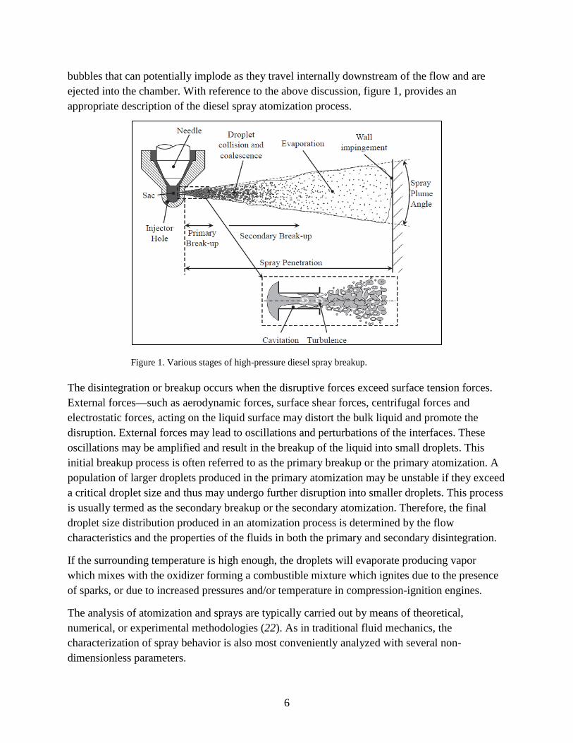
6
bubbles that can potentially implode as they travel internally downstream of the flow and are ejected into the chamber. With reference to the above discussion, figure 1, provides an appropriate description of the diesel spray atomization process.
Figure 1. Various stages of high-pressure diesel spray breakup.
The disintegration or breakup occurs when the disruptive forces exceed surface tension forces. External forces—such as aerodynamic forces, surface shear forces, centrifugal forces and electrostatic forces, acting on the liquid surface may distort the bulk liquid and promote the disruption. External forces may lead to oscillations and perturbations of the interfaces. These oscillations may be amplified and result in the breakup of the liquid into small droplets. This initial breakup process is often referred to as the primary breakup or the primary atomization. A population of larger droplets produced in the primary atomization may be unstable if they exceed a critical droplet size and thus may undergo further disruption into smaller droplets. This process is usually termed as the secondary breakup or the secondary atomization. Therefore, the final droplet size distribution produced in an atomization process is determined by the flow characteristics and the properties of the fluids in both the primary and secondary disintegration.
If the surrounding temperature is high enough, the droplets will evaporate producing vapor which mixes with the oxidizer forming a combustible mixture which ignites due to the presence of sparks, or due to increased pressures and/or temperature in compression-ignition engines.
The analysis of atomization and sprays are typically carried out by means of theoretical, numerical, or experimental methodologies (22). As in traditional fluid mechanics, the characterization of spray behavior is also most conveniently analyzed with several non-dimensionless parameters.
7
Several of the important parameters are listed below.
Liquid Reynolds number: 𝑅𝑒𝑙 =𝜌𝑙𝑢𝑙𝑑𝑙𝜇𝑙
(1) Liquid Weber number: 𝑊𝑒𝑙 =
𝜌𝑙𝑢𝑙2𝑑𝑙𝜎
(2) Aerodynamic (gas) Weber number: 𝑊𝑒𝑔 =
𝜌𝑔𝑢𝑟𝑒𝑙2 𝑑𝑙𝜎
(3)
Ohnesorge number:
𝑂ℎ = �𝑊𝑒𝑙𝑅𝑒𝑙
=𝜇𝑙
�𝜌𝑙𝜎𝑑𝑙 (4)
Discharge Coefficient: 𝐶𝑑 =
𝑣𝑙
�2∆𝑃𝜌𝑙
(5)
Cavitation Parameter:
𝐾 =2�𝑃𝑙 − 𝑃𝑔�𝜌𝑙𝑣2
(6)
3.1 Primary Atomization
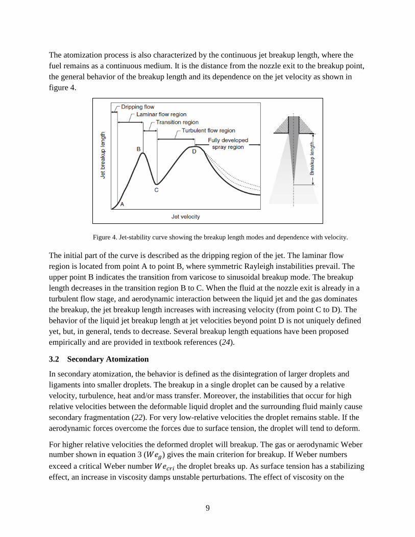
In primary breakup, the behavior of liquid sheets (or jets) can be classified into different atomization modes depending on boundary conditions. Figure 2 depicts the droplet breakup behavior with increasing Weber number conditions. Earlier investigation of single fluid pressure atomization, divided the breakup regimes of a circular liquid jet into three areas depending on the liquid Reynolds number and the Ohnesorge number (23). The regimes are further described below, and are also illustrated in figure 3.
1. At low-Reynolds number, the jet disintegrates due to surface tension effects into fairly identical droplet sizes (Rayleigh regime, symmetric, or varicose instability).
2. At intermediate-Reynolds number, drop formation is influenced by aerodynamics forces (non-axisymmetric Rayleigh breakup). These forces cause symmetric (first wind-induced mode) and asymmetric (second wind-induced mode, asymmetric or sinusoidal instability) wave growth of gas liquid interface that finally leads to jet disintegrations. This is known as the aerodynamic regime).
3. At higher-Reynolds number, the jet disintegrates almost spontaneously at the nozzle exit. This is called the atomization regime.
The transition line from the Rayleigh regime to the aerodynamic mode is identified by
𝑊𝑒𝑙 =1.74 × 10⁴
𝑅𝑒0.5 (7)
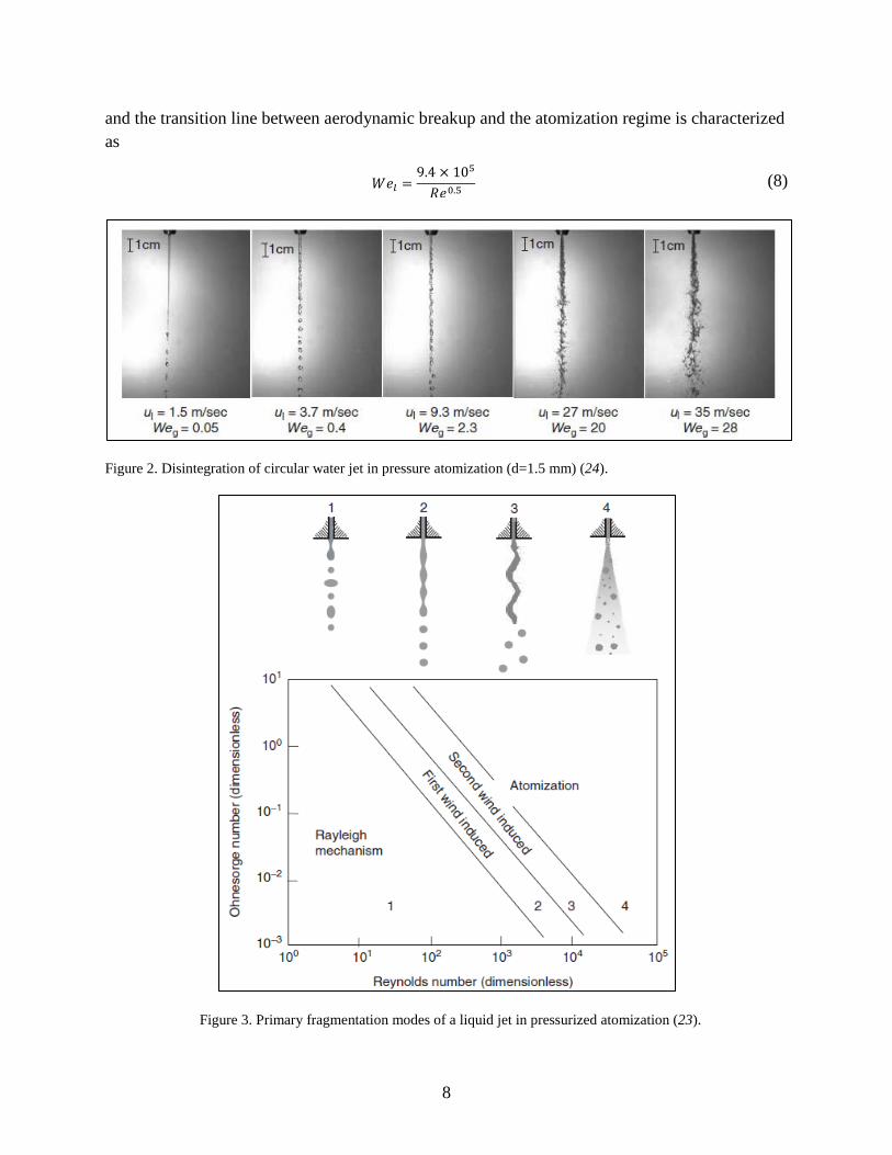
8
and the transition line between aerodynamic breakup and the atomization regime is characterized as
𝑊𝑒𝑙 =9.4 × 10⁵
𝑅𝑒0.5 (8)
Figure 2. Disintegration of circular water jet in pressure atomization (d=1.5 mm) (24).
Figure 3. Primary fragmentation modes of a liquid jet in pressurized atomization (23).
9
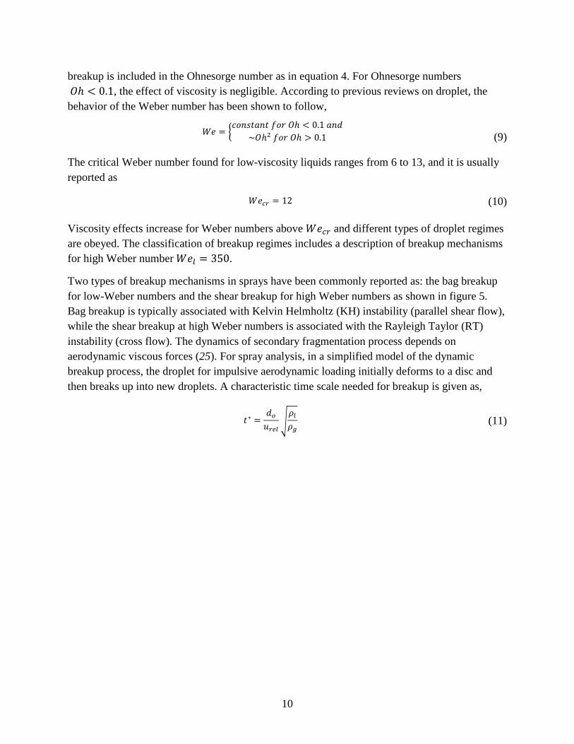
The atomization process is also characterized by the continuous jet breakup length, where the fuel remains as a continuous medium. It is the distance from the nozzle exit to the breakup point, the general behavior of the breakup length and its dependence on the jet velocity as shown in figure 4.
Figure 4. Jet-stability curve showing the breakup length modes and dependence with velocity.
The initial part of the curve is described as the dripping region of the jet. The laminar flow region is located from point A to point B, where symmetric Rayleigh instabilities prevail. The upper point B indicates the transition from varicose to sinusoidal breakup mode. The breakup length decreases in the transition region B to C. When the fluid at the nozzle exit is already in a turbulent flow stage, and aerodynamic interaction between the liquid jet and the gas dominates the breakup, the jet breakup length increases with increasing velocity (from point C to D). The behavior of the liquid jet breakup length at jet velocities beyond point D is not uniquely defined yet, but, in general, tends to decrease. Several breakup length equations have been proposed empirically and are provided in textbook references (24).
3.2 Secondary Atomization
In secondary atomization, the behavior is defined as the disintegration of larger droplets and ligaments into smaller droplets. The breakup in a single droplet can be caused by a relative velocity, turbulence, heat and/or mass transfer. Moreover, the instabilities that occur for high relative velocities between the deformable liquid droplet and the surrounding fluid mainly cause secondary fragmentation (22). For very low-relative velocities the droplet remains stable. If the aerodynamic forces overcome the forces due to surface tension, the droplet will tend to deform.
For higher relative velocities the deformed droplet will breakup. The gas or aerodynamic Weber number shown in equation 3 (𝑊𝑒𝑔) gives the main criterion for breakup. If Weber numbers exceed a critical Weber number 𝑊𝑒𝑐𝑟𝑖 the droplet breaks up. As surface tension has a stabilizing effect, an increase in viscosity damps unstable perturbations. The effect of viscosity on the
10
breakup is included in the Ohnesorge number as in equation 4. For Ohnesorge numbers 𝑂ℎ < 0.1, the effect of viscosity is negligible. According to previous reviews on droplet, the behavior of the Weber number has been shown to follow,
𝑊𝑒 = �𝑐𝑜𝑛𝑠𝑡𝑎𝑛𝑡 𝑓𝑜𝑟 𝑂ℎ < 0.1 𝑎𝑛𝑑
~𝑂ℎ2 𝑓𝑜𝑟 𝑂ℎ > 0.1�
(9)
The critical Weber number found for low-viscosity liquids ranges from 6 to 13, and it is usually reported as
𝑊𝑒𝑐𝑟 = 12 (10) Viscosity effects increase for Weber numbers above 𝑊𝑒𝑐𝑟 and different types of droplet regimes are obeyed. The classification of breakup regimes includes a description of breakup mechanisms for high Weber number 𝑊𝑒𝑙 = 350.
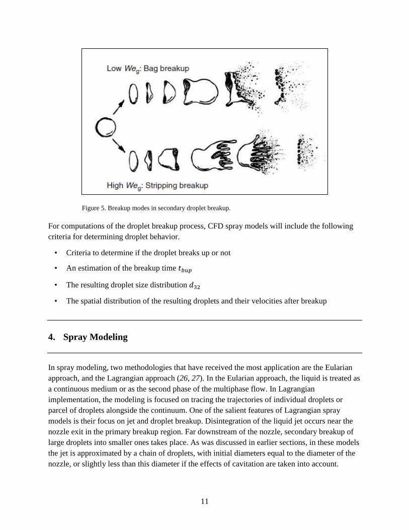
Two types of breakup mechanisms in sprays have been commonly reported as: the bag breakup for low-Weber numbers and the shear breakup for high Weber numbers as shown in figure 5. Bag breakup is typically associated with Kelvin Helmholtz (KH) instability (parallel shear flow), while the shear breakup at high Weber numbers is associated with the Rayleigh Taylor (RT) instability (cross flow). The dynamics of secondary fragmentation process depends on aerodynamic viscous forces (25). For spray analysis, in a simplified model of the dynamic breakup process, the droplet for impulsive aerodynamic loading initially deforms to a disc and then breaks up into new droplets. A characteristic time scale needed for breakup is given as,
𝑡∗ =
𝑑𝑜𝑢𝑟𝑒𝑙
�𝜌𝑙𝜌𝑔
(11)
11
Figure 5. Breakup modes in secondary droplet breakup.
For computations of the droplet breakup process, CFD spray models will include the following criteria for determining droplet behavior.
• Criteria to determine if the droplet breaks up or not
• An estimation of the breakup time 𝑡𝑏𝑢𝑝
• The resulting droplet size distribution 𝑑32
• The spatial distribution of the resulting droplets and their velocities after breakup
4. Spray Modeling
In spray modeling, two methodologies that have received the most application are the Eularian approach, and the Lagrangian approach (26, 27). In the Eularian approach, the liquid is treated as a continuous medium or as the second phase of the multiphase flow. In Lagrangian implementation, the modeling is focused on tracing the trajectories of individual droplets or parcel of droplets alongside the continuum. One of the salient features of Lagrangian spray models is their focus on jet and droplet breakup. Disintegration of the liquid jet occurs near the nozzle exit in the primary breakup region. Far downstream of the nozzle, secondary breakup of large droplets into smaller ones takes place. As was discussed in earlier sections, in these models the jet is approximated by a chain of droplets, with initial diameters equal to the diameter of the nozzle, or slightly less than this diameter if the effects of cavitation are taken into account.
12
This section aims at providing several models for separate treatment of these two regions or models for combined treatment.
4.1 The Spray Equation: A Statistical Description
A statistical description for the stochastic behavior of spray was introduced on the landmark paper by Williams (28). This mathematical model includes the effects of droplet growth, the formation of new droplets, collisions, and aerodynamics forces. In principle, for sprays composed of 𝑁 particles, a statistical description will involve the specification of the 𝑁𝑡ℎ order distribution function in the phase space consisting of 3𝑁 spatial coordinates and 3𝑁 velocity coordinates. In the probability density approach, the spray droplets are represented by a PDF,𝑓(𝑡, 𝑥,𝑦, 𝑧), representing the probable number of droplets per unit volume in time and space. The state of the droplet is described by its parameters that are the coordinates in the particle state space, the parameters typically are: location 𝑥, velocity 𝑣, radius 𝑟 , the temperature 𝑇𝑑 , the deformation parameter and rate of deformation, 𝑦, �̇�, respectively.
The spray PDF is the solution of a spray transport equation given in component form as,
𝑑𝑓𝑑𝑡
+ 𝑑𝑖𝑣𝑥(𝑓𝑣) + 𝑑𝑖𝑣𝑦(𝑓𝑣)̇ +𝜕𝜕𝑟
(𝑓�̇�) +𝜕𝜕𝑇𝑑
�𝑓𝑇�̇�� +𝜕𝜕𝑦
(𝑓�̇�) +𝜕𝜕�̇�
(𝑓�̈�) = 𝑓𝑐𝑜𝑙𝑙̇ + 𝑓𝑏𝑢̇ (12) where the source terms are due to droplet collision and breakup and are modeled via individual spray sub processes. Additional models also need to be available for each subprocess on the left hand side of equation 10 for a complete description of the spray physics.
In this next section, models are presented to account for droplet acceleration, droplet radius, droplet temperature, droplet deformation, droplet collision, and droplet breakup (atomization) for use in contemporary spray solvers (29).
4.1.1 Droplet Acceleration
The droplet acceleration equation of motion is given by,
𝑑𝑑𝑡𝐯 =
38𝐶𝑑𝜌𝑔𝜌𝑙
||𝐯𝐫||𝑟
𝐯𝐫 + 𝐠 (13) where 𝐶𝑑 is the drag coefficient, 𝜌𝑔, 𝜌𝑙 the gas and liquid densities, 𝐯𝐫 is the relative drop velocity defined as 𝐯𝐫 = 𝐮 + 𝐮′ − 𝐯 accounting for turbulence fluctuations, and 𝐠 is the gravitational constant. The drag coefficient is given by following formulas,
𝐶𝑑 = �24𝑅𝑒𝑑
�1 + 𝑅𝑒𝑑2/3/6� if 𝑅𝑒𝑑 ≤ 1000
0.424 if 𝑅𝑒𝑑 > 1000�
where 𝑅𝑒𝑑 is the droplet Reynolds number defined by, 𝑅𝑒𝑑 = 2𝑟𝜌𝑔𝐯𝐫/𝜇𝑔(𝑇�), and the weighted gas temperature is given by the two third law, 𝑇� = (𝑇 + 2𝑇𝑑)/3.
13
4.1.2 Drop Radius
Considering mainly for convective heat and mass transfer, the Frossling correlation is used to determine the droplet radius. It is determined from the mass rate of change due to evaporation or condensation, its expression is written as,
𝑑𝑑𝑡𝑟2 =
𝜌𝑣𝜌𝑑𝐷𝑣𝐵𝑑𝑆ℎ𝑑 (14)
where 𝐷𝑣 is the vapor diffusivity in the gas and it is determined from the empirical Frossling correlation, 𝜌𝑣𝐷𝑣 = 𝐷1𝑇�𝐷2 having 𝐷1 and 𝐷2 as constants and 𝑇� . The Spalding mass transfer number is used to define,
𝐵𝑑 = (𝑌𝑣∗ − 𝑌𝑣)/(1 − 𝑌𝑣∗) (15)
and 𝑌𝑣 = 𝜌𝑣/𝜌𝑔 is the vapor mass fraction, and 𝑌𝑣∗ is the vapor mass fraction on the drop surface calculated assuming equilibrium conditions and invoking the Clayperon thermodynamic equation,
𝑌𝑣∗(𝑇𝑑) = �1 +
𝑀𝑊𝑠
𝑀𝑊𝑣�
𝑝𝑔𝑝𝑣(𝑇𝑑) − 1��
−1
(16)
The molecular weights are denoted as 𝑀𝑊𝑠, for the surrounding gas, and 𝑀𝑊𝑣 for the vapor. The equilibrium vapor pressure is denoted as, 𝑝𝑣(𝑇𝑑) and 𝑝𝑔is the gas pressure.
The Sherwood number is denoted as
𝑆ℎ𝑑 = �2.0 + 0.6𝑅𝑒𝑑1/2𝑆𝑐𝑑
1/3 �𝑙𝑛1 + 𝐵𝑑𝐵𝑑
(17)
where the droplet Schmidt number is defined as, 𝑆𝑐𝑑 = 𝜇(𝑇�)/𝜌𝑔𝐷𝑔(𝑇�).
4.1.3 Drop Temperature
An energy balance determines the rate of change of the droplet temperature, where the energy supplied to the drop raises the temperature or supplies heat for evaporation. The mathematical expression is written as,
𝐶𝑑𝑚𝑑𝑑𝑇𝑑𝑑𝑡
= 𝑞ℎ𝑆𝑑 + 𝐿(𝑇𝑑)𝑑𝑚𝑑
𝑑𝑡 (18)
where 𝐶𝑑 is the droplet specific heat, 𝑚𝑑 the mass, 𝑆𝑑 the surface, 𝑞ℎ is the convective heat transferred to the drop, and 𝐿(𝑇𝑑) is the latent heat of evaporation. The change in droplet temperature heat conduction rate, 𝑞ℎ , is given by the Ranz-Marshall correlation as follows,
14
𝑞ℎ = 𝐾𝑔�𝑇��𝑁𝑢𝑑(𝑇 − 𝑇𝑑)/2𝑟 (19) The conductivity of the gas is given by the empirical relationship 𝐾𝑔�𝑇�� = �𝐾1𝑇�
32� /�𝑇� + 𝐾2�,
where 𝐾1 and 𝐾2 are constants. The convective heat transfer is expressed in terms of Nusselt number as,
𝑁𝑢𝑑 = �2.0 + 0.6𝑅𝑒𝑑1/2Prd
1/3 �𝑙𝑛1 +𝐵𝑑𝐵𝑑
(20)
where 𝑅𝑒𝑑is the droplets Reynolds number and the droplet Prandlt number is defined by 𝑃𝑟𝑑 = 𝜇𝑔�𝑇��𝐶𝑝(𝑇�)/𝐾𝑔�𝑇��. Finally the latent heat of vaporization is defined as the difference between the vapor enthalpy ℎ𝑣 and the liquid enthalpy ℎ𝑑 as,
𝐿(𝑇𝑑) = ℎ𝑣(𝑇𝑑) − ℎ𝑑�𝑇𝑑 , 𝑝𝑣(𝑇𝑑)� = �𝑒𝑣(𝑇𝑑) +
𝑅𝑜𝑇𝑑𝑀𝑊𝑣
� − �𝑒𝑑(𝑇𝑑) +𝑝𝑣(𝑇𝑑)𝜌𝑑
� (21) where 𝑒 is the specific internal heat, 𝑅𝑜 the universal gas constant, 𝑀𝑊𝑣 the molecular weight of the vapor, and 𝑝𝑣(𝑇𝑑) is the equilibrium vapor pressure.
4.1.4 Drop Deformation
Drop distortion is important in the determination of breakup in atomization process. Typically deformation is modeled by use of Taylor’s drop oscillator (TAB model) where distortion is described by a forced, damped, harmonic oscillator. The forcing term is given by the aerodynamic drag, the damping is due to the liquid viscosity, and surface tension is the restoring force. The deformation equation is written as,
�̈� = 𝐶𝐹𝐶𝐵𝜌𝑔𝜌𝑙𝑢2
𝑟2 −𝐶𝐾𝜎𝜌𝑙𝑟3𝑦−
𝐶𝑑𝜇𝑙𝜌𝑙𝑟2 �̇� (22)
where 𝐶𝐹 ,𝐶𝐾, and 𝐶𝑑 are dimensionless numbers, further details of this model is given in section 4.2.4.
4.1.5 Drop Collisions
The droplet collision model of O’Rourke and Amsden (36) is consistent with the stochastic nature of spray simulations, where only a subsample of droplets is tracked. It represents parcels of varying number of drops. The size, number, and velocity of parcels determine the probability of colliding with other parcels. The drop collisions are accounted via the source term 𝑓𝑐𝑜𝑙𝑙̇ .The probability for a drop with index 1 to undergo collisions with a drop of index 2 in a given volume 𝑉 during a specified time interval ∆𝑡 is given by the Poisson distribution,
𝑃𝑛 = �̅�𝑛𝑒𝑥𝑝(−�̅�)/𝑛! (23)
15
where �̅� = 𝜈∆𝑡 is the mean. The collision frequency is modeled as,
𝜈 =𝑁2𝑉𝜋(𝑟1 + 𝑟2)2‖𝐯𝟏 − 𝐯𝟐‖ (24)
where 𝑁2 represents the number of drops in volume and drop state 2. The collision in this model will have two possible outcomes, depending on the collision impact parameter b; for cases when 𝑏 < 𝑏𝑐𝑟 then the drop will coalesce, and if 𝑏 > 𝑏𝑐𝑟 then the drops undergo an elastic collision (rebound) maintaining their size and temperature. The critical impact parameter 𝑏𝑐𝑟 = 𝑏𝑐𝑟(𝑟1, 𝑟2,𝜎) depends on collision drop sizes and surface tension, 𝜎.
Other techniques for modeling droplet collision include the works proposed by Schmidt and Rutland (30), it is based on the No Time Counter (NTC) method used in gas dynamics for Direct Numerical Simulation calculations.
4.2 Review of Liquid Spray Breakup Models
Typically fuel injection is handled using a blob injection model and due to the interaction with the environment the computational parcels are subject to surface instabilities.
In diesel spray applications, the instabilities are typically described through KH and RT models, which are used to predict primary and secondary breakup. An intact liquid-core breakup length is used where the KH model alone is used to predict primary breakup; downstream of this critical length (and in the hybrid case) the RT and KH models are implemented in competing manners, such that the droplet breaks up by the model that predicts a shorter breakup time. In the injector nozzle region, where droplet velocities are larger, the RT breakup model dominates, while in KH model is used further downstream.
The section will describe in detail some of the leading engine spray models.
4.2.1 KH Breakup Model
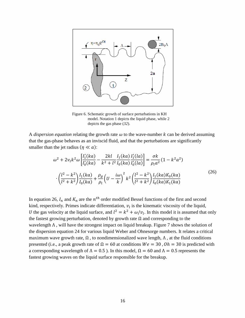
The formulation of the KH Wave Breakup Model developed primarily by Reitz and Diwaker (31) considers a cylindrical liquid jet of radius a penetrating through a circular orifice into a quiescent incompressible gas chamber. The interaction between the surrounding gas and the liquid jet creates a number of infinitesimal surface perturbations that are characterized with initial amplitude of 𝜂𝑜and a spectrum of wavelengths 𝜆 (𝑘 = 2𝜋/𝜆), see figure 6. The perturbation amplitude increases exponentially due to the interaction between the liquid and the gas; the growth rate is complex and is described as 𝜔 = 𝜔𝑟 + 𝑖𝜔𝑖. The surface perturbations are described with the following relation:
𝜂(𝑡) = 𝑅(𝜂𝑜exp [𝑖𝑘𝑥 + 𝜔])) (25)
16
Figure 6. Schematic growth of surface perturbations in KH model. Notation 1 depicts the liquid phase, while 2 depicts the gas phase (32).
A dispersion equation relating the growth rate 𝜔 to the wave-number 𝑘 can be derived assuming that the gas-phase behaves as an inviscid fluid, and that the perturbations are significantly smaller than the jet radius (𝜂 ≪ 𝑎):
𝜔2 + 2𝜈𝑙𝑘2𝜔 �
𝐼1′(𝑘𝑎)𝐼0′(𝑘𝑎) −
2𝑘𝑙𝑘2 + 𝑙2
𝐼1(𝑘𝑎)𝐼0(𝑘𝑎)
𝐼1′(𝑙𝑎)𝐼0′(𝑙𝑎)� =
𝜎𝑘𝜌𝑙𝑎2
(1 − 𝑘2𝑎2)
∙ �𝑙2 − 𝑘2
𝑙2 + 𝑘2�𝐼1(𝑘𝑎)𝐼0(𝑘𝑎) +
𝜌𝑔𝜌𝑙�𝑈 −
𝑖𝜔𝑘�2
𝑘2 �𝑙2 − 𝑘2
𝑙2 + 𝑘2�𝐼1(𝑘𝑎)𝐾0(𝑘𝑎)𝐼0(𝑘𝑎)𝐾1(𝑘𝑎)
(26)
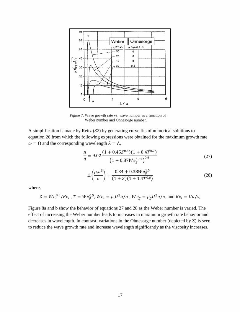
In equation 26, 𝐼𝑛 and 𝐾𝑛 are the 𝑛𝑡ℎ order modified Bessel functions of the first and second kind, respectively. Primes indicate differentiation, 𝑣𝑙 is the kinematic viscosity of the liquid, 𝑈 the gas velocity at the liquid surface, and 𝑙2 = 𝑘2 + 𝜔/𝑣𝑙. In this model it is assumed that only the fastest growing perturbation, denoted by growth rate Ω and corresponding to the wavelength Λ , will have the strongest impact on liquid breakup. Figure 7 shows the solution of the dispersion equation 24 for various liquid Weber and Ohnesorge numbers. It relates a critical maximum wave growth rate, Ω , to nondimensionalized wave length, Λ , at the fluid conditions presented (i.e., a peak growth rate of Ω = 60 at conditions 𝑊𝑒 = 30 ,𝑂ℎ = 30 is predicted with a corresponding wavelength of Λ = 0.5 ). In this model, Ω = 60 and Λ = 0.5 represents the fastest growing waves on the liquid surface responsible for the breakup.
17
Figure 7. Wave growth rate vs. wave number as a function of Weber number and Ohnesorge number.
A simplification is made by Reitz (32) by generating curve fits of numerical solutions to equation 26 from which the following expressions were obtained for the maximum growth rate 𝜔 = Ω and the corresponding wavelength 𝜆 = Λ,
Λ𝑎
= 9.02(1 + 0.45𝑍0.5)(1 + 0.4𝑇0.7)
�1 + 0.87𝑊𝑒𝑔1.67�0.6 (27)
Ω�𝜌𝑙𝑎3
𝜎� =
0.34 + 0.38𝑊𝑒𝑔1.5
(1 + 𝑍)(1 + 1.4𝑇0.6) (28)
where,
𝑍 = 𝑊𝑒𝑙0.5/𝑅𝑒𝑙 , 𝑇 = 𝑊𝑒𝑔0.5, 𝑊𝑒𝑙 = 𝜌𝑙𝑈2𝑎/𝜎 , 𝑊𝑒𝑔 = 𝜌𝑔𝑈2𝑎/𝜎, and 𝑅𝑒𝑙 = 𝑈𝑎/𝜈𝑙
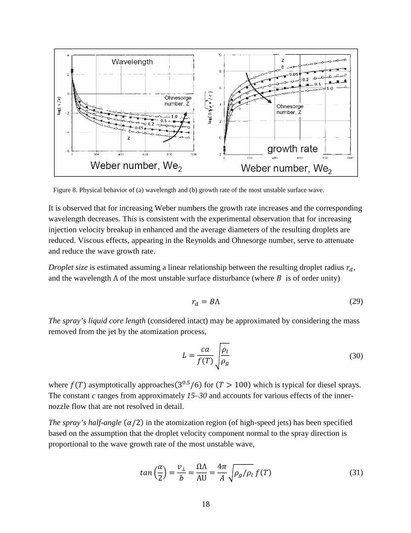
Figure 8a and b show the behavior of equations 27 and 28 as the Weber number is varied. The effect of increasing the Weber number leads to increases in maximum growth rate behavior and decreases in wavelength. In contrast, variations in the Ohnesorge number (depicted by Z) is seen to reduce the wave growth rate and increase wavelength significantly as the viscosity increases.
18
Figure 8. Physical behavior of (a) wavelength and (b) growth rate of the most unstable surface wave.
It is observed that for increasing Weber numbers the growth rate increases and the corresponding wavelength decreases. This is consistent with the experimental observation that for increasing injection velocity breakup in enhanced and the average diameters of the resulting droplets are reduced. Viscous effects, appearing in the Reynolds and Ohnesorge number, serve to attenuate and reduce the wave growth rate.
Droplet size is estimated assuming a linear relationship between the resulting droplet radius 𝑟𝑑, and the wavelength Λ of the most unstable surface disturbance (where 𝐵 is of order unity)
𝑟𝑑 = 𝐵Λ (29) The spray’s liquid core length (considered intact) may be approximated by considering the mass removed from the jet by the atomization process,
𝐿 =
𝑐𝑎𝑓(𝑇)�
𝜌𝑙𝜌𝑔
(30)
where 𝑓(𝑇) asymptotically approaches(30.5/6) for (𝑇 > 100) which is typical for diesel sprays. The constant c ranges from approximately 15–30 and accounts for various effects of the inner-nozzle flow that are not resolved in detail.
The spray’s half-angle (𝛼/2) in the atomization region (of high-speed jets) has been specified based on the assumption that the droplet velocity component normal to the spray direction is proportional to the wave growth rate of the most unstable wave,
𝑡𝑎𝑛 �𝛼2� =
𝑣⊥𝑏
=ΩΛAU
=4𝜋𝐴 �𝜌𝑔/𝜌𝑙 𝑓(𝑇) (31)
19
where the constant A accounts for the nozzle geometry and it has been defined in terms of the length to diameter ratio of the nozzle hole,
𝐴 = 3.0 +
𝑙𝑛𝑜𝑧/𝑑𝑛𝑜𝑧3.6
(32)
4.2.2 Blob Injection Model
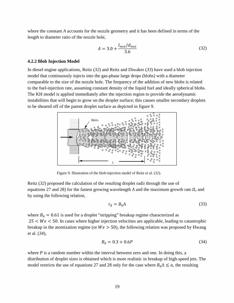
In diesel engine applications, Reitz (32) and Reitz and Diwaker (33) have used a blob injection model that continuously injects into the gas-phase large drops (blobs) with a diameter comparable to the size of the nozzle hole. The frequency of the addition of new blobs is related to the fuel-injection rate, assuming constant density of the liquid fuel and ideally spherical blobs. The KH model is applied immediately after the injection region to provide the aerodynamic instabilities that will begin to grow on the droplet surface; this causes smaller secondary droplets to be sheared off of the parent droplet surface as depicted in figure 9.
Figure 9. Illustration of the blob-injection model of Reitz et al. (32).
Reitz (32) proposed the calculation of the resulting droplet radii through the use of equations 27 and 28) for the fastest growing wavelength Λ and the maximum growth rate Ω, and by using the following relation,
𝑟𝑑 = 𝐵0Λ (33) where 𝐵0 = 0.61 is used for a droplet “stripping” breakup regime characterized as 25 < 𝑊𝑒 < 50. In cases where higher injection velocities are applicable, leading to catastrophic breakup in the atomization regime (or 𝑊𝑒 > 50), the following relation was proposed by Hwang et al. (34),
𝐵0 = 0.3 + 0.6𝑃 (34) where P is a random number within the interval between zero and one. In doing this, a distribution of droplet sizes is obtained which is more realistic in breakup of high-speed jets. The model restricts the use of equations 27 and 28 only for the case where 𝐵0Λ ≤ 𝑎, the resulting
20
droplet diameter is less than the radius of the original drop. When this condition is not satisfied, 𝑟𝑑 is estimated as,
𝑟𝑑 = 𝑚𝑖𝑛 �
(3𝜋𝑎2𝑈/2Ω)1/3
(3𝑎2Λ/4)1/3� for 𝐵0Λ > 𝑎, calculated once
(35)
Equation 35 is based on the assumption that the jet disturbance has a frequency of 𝑓 = Ω/2𝜋 (i.e., one drop is formed each wave period), or that droplet size is determined from the volume of liquid contained under one surface wave.
The breakup and generation of new small droplets lead to a reduction in size of the original blob. A mathematical description of the temporal change in radius of the parent drop is written as,
𝑑𝑎𝑑𝑡
= −𝑎 − 𝑟𝑏𝜏
(36)
where 𝜏 is the breakup time given as,
𝜏 = 3.726𝐵1𝑎ΛΩ
(37)
and the constant 𝐵1 is introduced to account for internal flow effects of the nozzle flow on the breakup time. Reitz and Diwaker (31, 33) suggests using a value 𝐵1 = 20 where other references report more accurate values with values ranging from 𝐵1 = 1.73 up to 𝐵1 = 30. To reproduce the spray cone angle the child droplets emanating from the blobs have a velocity component perpendicular to the main spray orientation. Maximum values of this component are obtained from the spray half-angle specified in equation 29. It also suggests using an even distribution between zero and the maximum normal velocity for the various droplets in order to achieve a realistic droplet density within the spray.
Additionally, it is also shown that in the limits 𝑊𝑒 → 0 and 𝑊𝑒 → ∞ the characteristic breakup time, 𝜏 , takes the form of,
𝜏 =
⎩⎪⎨
⎪⎧
0.82𝐵1�𝜌𝑙𝑟03
𝜎 ,𝑓𝑜𝑟 𝑏𝑎𝑔 𝑏𝑟𝑒𝑎𝑘𝑢𝑝
𝐵1�𝜌𝑙𝜌𝑔
𝑟0|𝑈| ,𝑓𝑜𝑟 𝑠ℎ𝑒𝑎𝑟 𝑏𝑟𝑒𝑎𝑘𝑢𝑝
�
(38)
Conditions for bag and shear breakup are experimentally determined and reported to be 𝑊𝑒 >6 and 𝑊𝑒/�𝑅𝑒𝐺 > 0.5 , respectively, with the Weber and Reynolds number based on the droplet radius.
21
4.2.3 Linearized Instability Sheet Atomization (LISA) Breakup Model
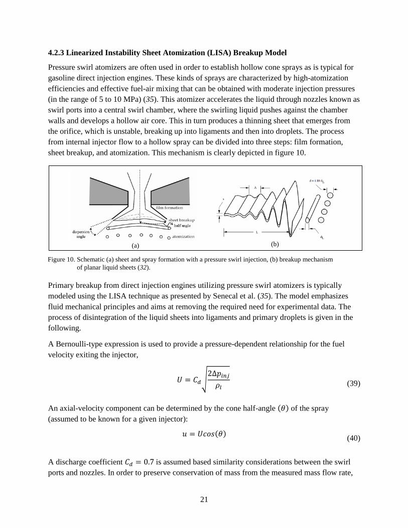
Pressure swirl atomizers are often used in order to establish hollow cone sprays as is typical for gasoline direct injection engines. These kinds of sprays are characterized by high-atomization efficiencies and effective fuel-air mixing that can be obtained with moderate injection pressures (in the range of 5 to 10 MPa) (35). This atomizer accelerates the liquid through nozzles known as swirl ports into a central swirl chamber, where the swirling liquid pushes against the chamber walls and develops a hollow air core. This in turn produces a thinning sheet that emerges from the orifice, which is unstable, breaking up into ligaments and then into droplets. The process from internal injector flow to a hollow spray can be divided into three steps: film formation, sheet breakup, and atomization. This mechanism is clearly depicted in figure 10.
Figure 10. Schematic (a) sheet and spray formation with a pressure swirl injection, (b) breakup mechanism
of planar liquid sheets (32).
Primary breakup from direct injection engines utilizing pressure swirl atomizers is typically modeled using the LISA technique as presented by Senecal et al. (35). The model emphasizes fluid mechanical principles and aims at removing the required need for experimental data. The process of disintegration of the liquid sheets into ligaments and primary droplets is given in the following.
A Bernoulli-type expression is used to provide a pressure-dependent relationship for the fuel velocity exiting the injector,
𝑈 = 𝐶𝑑�
2∆𝑝𝑖𝑛𝑗𝜌𝑙
(39)
An axial-velocity component can be determined by the cone half-angle (𝜃) of the spray (assumed to be known for a given injector):
𝑢 = 𝑈𝑐𝑜𝑠(𝜃) (40)
A discharge coefficient 𝐶𝑑 = 0.7 is assumed based similarity considerations between the swirl ports and nozzles. In order to preserve conservation of mass from the measured mass flow rate,
(a) (b)
22
�̇�𝑖𝑛𝑗, Reitz (32) suggests to enforce the following expression (discharge coefficients taking values below 0.7 are assumed to be representative of an air-core existing in the center of the rotating flow)
𝐶𝑑 = 𝑚𝑎𝑥 �0.7,
4�̇�𝑖𝑛𝑗
𝜋𝑑𝑛𝑜𝑧2 𝜌𝑙 cos(𝜃)�𝜌𝑙
2∆𝑝𝑖𝑛𝑗 �
(41)
The continuity equation relating the thickness 𝑡𝑓 of the liquid film inside the injector to the measured mass flow rate is given as,
�̇�𝑖𝑛𝑗 = 𝜋𝑢𝑡𝑓�𝑑𝑛𝑜𝑧 − 𝑡𝑓� (42) Following the same assumptions as the KH wave breakup model, a spectrum of infinitesimal disturbances imposed on the liquid-sheet surface from the liquid-gas interaction causing the amplitudes of the waves to grow as in equation 23, 𝜂(𝑡) = 𝑅(𝜂𝑜exp [𝑖𝑘𝑥 + 𝜔]). Similarly, the most unstable disturbance having the largest value of 𝜔𝑟, denoted by Ω, is assumed to be responsible for sheet breakup and an expression for a dispersion relation, 𝜔𝑟 = 𝜔𝑟(𝑘), is clearly needed to extract this parameter. Senecal et al. (35) provided a simplified dispersion relationship assuming sinuous wave mode disturbances on the liquid sheet surfaces (waves traveling on both surfaces of the liquid sheet travel exactly in phase),
𝜔𝑟 = −2𝜈𝑙𝑘2 + �4𝜈𝑙2𝑘4 +
𝜌𝑔𝜌𝑙𝑈2𝑘2 −
𝜎𝑘3
𝜌𝑙 (43)
Equation 43 provides a dispersion relation (for sinuous-wave mode surface disturbances) that can be obtained under the following assumptions: (1) using an order of magnitude analysis from the inviscid solutions to show that the second order terms in viscosity can be neglected in comparison to other terms; (2) for cases where Weber numbers of 𝑊𝑒𝑔 = 27/16 is exceeded, short waves will grow on the sheet surface, with a growth rate independent of the sheet thickness; (3) the gas-to-liquid density ration has to meet the condition, 𝜌𝑔/𝜌𝑙 ≪ 1.
The breakup time used to calculate the critical amplitude of surface disturbances (the time where ligaments are assumed to be formed) is provided as,
𝜂𝑏 = 𝜂0𝑒𝑥𝑝(Ω𝜏𝑏)
𝜏𝑏 =1𝑎
ln �𝜂𝑏𝜂0�
(44)
23
where 𝜂𝑏 is the critical amplitude at breakup, 𝜂0is the amplitude of the initial disturbance, and Ω is the maximum growth rate that is obtained by numerically maximizing equation 26 as a function of the wave number 𝑘 .
The breakup length 𝐿 is now estimated by assuming constant velocity for the liquid sheet,
𝐿 = 𝑈𝜏𝑏 =
𝑈Ω𝑙𝑛 �
𝜂𝑏𝜂0�
(45)
where quantity 𝜂𝑏/𝜂0 has been reported as 𝜂𝑏/𝜂0 = 12.
Ligament diameter formed at the breakup point is obtained from a mass balance, assuming that the ligaments are formed from tears in the sheet once per wavelength. The resulting diameter is given as,
𝑑𝐿 = �4
𝜋Λs ∙ 2ℎ = �
16ℎ𝐾𝑠
(46)
where 𝐾𝑠 is the wavenumber 𝐾𝑠 = 2𝜋/Λs corresponding to the maximum growth rate Ω leading to the breakup of the sheet. The ligament diameter is a function of the sheet half-thickness ℎ at the breakup position, which is related to its initial value ℎ0 at the nozzle orifice by,
ℎ =
ℎ0�𝑑𝑛𝑜𝑧 − 𝑡𝑓�2𝐿 𝑠𝑖𝑛(𝜃)𝑑𝑛𝑜𝑧 − 𝑡𝑓
(47)
and
ℎ0 ≈𝑡𝑓2
cos(𝜃) (48)
Further breakup of ligaments into droplets is calculated based on an analogy to Weber’s result for growing waves on cylindrical, viscous liquid columns. The wave number 𝐾𝐿 for the fastest growing wave on the ligament is,
𝐾𝐿𝑑𝐿 = �
12
+3𝜇𝑙
2�𝜌𝑙𝜎𝑑𝐿�1/2
(49)
24
Assuming that breakup occurs when the amplitude of the most unstable wave is equal to the radius of the ligament (one drop will be formed per wavelength). A mass balance then yields an expression for the droplet diameter, 𝑑𝑑𝑟𝑜𝑝
𝑑𝑑𝑟𝑜𝑝 = �
3𝜋𝑑𝐿2
𝐾𝐿�1/3
(50)
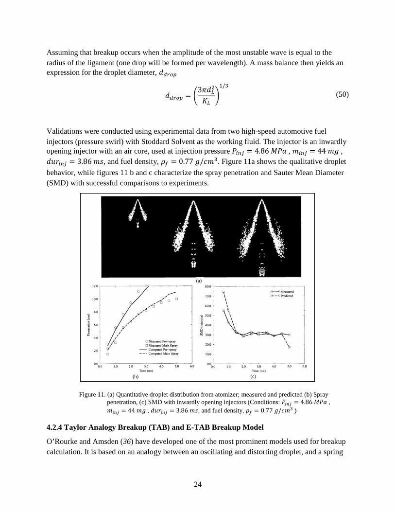
Validations were conducted using experimental data from two high-speed automotive fuel injectors (pressure swirl) with Stoddard Solvent as the working fluid. The injector is an inwardly opening injector with an air core, used at injection pressure 𝑃𝑖𝑛𝑗 = 4.86 𝑀𝑃𝑎 , 𝑚𝑖𝑛𝑗 = 44 𝑚𝑔 , 𝑑𝑢𝑟𝑖𝑛𝑗 = 3.86 𝑚𝑠, and fuel density, 𝜌𝑓 = 0.77 𝑔/𝑐𝑚3. Figure 11a shows the qualitative droplet behavior, while figures 11 b and c characterize the spray penetration and Sauter Mean Diameter (SMD) with successful comparisons to experiments.
Figure 11. (a) Quantitative droplet distribution from atomizer; measured and predicted (b) Spray penetration, (c) SMD with inwardly opening injectors (Conditions: 𝑃𝑖𝑛𝑗 = 4.86 𝑀𝑃𝑎 , 𝑚𝑖𝑛𝑗 = 44 𝑚𝑔 , 𝑑𝑢𝑟𝑖𝑛𝑗 = 3.86 𝑚𝑠, and fuel density, 𝜌𝑓 = 0.77 𝑔/𝑐𝑚3 )
4.2.4 Taylor Analogy Breakup (TAB) and E-TAB Breakup Model
O’Rourke and Amsden (36) have developed one of the most prominent models used for breakup calculation. It is based on an analogy between an oscillating and distorting droplet, and a spring
(a)
(b) (c)
25
mass system. The restoring force of the spring corresponds to the surface tension forces, external forces on the mass corresponds to the aerodynamic drag forces, and the damping force is represented by the viscosity of the liquid. The formulation of the classical TAB model is given below,
The equation of the damped, forced harmonic oscillator is given by:
𝑚�̈� = 𝐹 − 𝑘𝑠𝑥 − 𝑑�̇� (51) where 𝑥 is the displacement (droplet displacement from equilibrium), 𝐹 are the external forces (drag), 𝑘𝑠 is the spring constant (surface tension), and 𝑑 is the damping parameter (liquid viscosity). With the use of Taylor’s analogy, the physical dependencies of the coefficients are
𝐹𝑚
= 𝐶𝐹𝜌𝑔𝑢2
𝜌𝑙𝑟 ,𝑘𝑠𝑚
= 𝐶𝐾𝜎𝜌𝑙𝑟3
,𝑑𝑚
= 𝐶𝑑𝜇𝑙𝜌𝑙𝑟2
(52)
where 𝐶𝐹 ,𝐶𝐾, and 𝐶𝑑 are dimensionless numbers. Additionally, 𝐶𝐵 is used to normalize 𝑥, 𝑦 = 𝑥/𝐶𝐵𝑟 and normalizing the oscillator equation yields,
�̈� =
𝐶𝐹𝐶𝐵
𝜌𝑔𝜌𝑙𝑢2
𝑟2−𝐶𝐾𝜎𝜌𝑙𝑟3
𝑦 −𝐶𝑑𝜇𝑙𝜌𝑙𝑟2
�̇� (53)
with breakup occurring if and only if 𝑦 > 1, and if and only if the amplitude of oscillation of the north and south poles equals the drop radius. The dimensionless constants, 𝐶𝐹 ,𝐶𝐾,𝑎𝑛𝑑 𝐶𝑑, are determined by comparing with experimental and theoretical results and have the following values: 𝐶𝐾 = 8, 𝐶𝑑 = 0.5, 𝐶𝑏 = 0.5 , and 𝐶𝐹 = 1/3. We also note that it has been reported by Grover et al. (37) that for gasoline sprays a value of 𝐶𝐾 = 0.6 resulted in better agreement with measurements; thus the need for model parameter calibration for different fuels is clearly needed.
The prediction of droplet sizes after breakup is based upon an energy conservation analysis. In the analysis, a balance of the energy of the parent drop with the energies of the newly generated drops after breakup carried out to yield,
𝑟𝑟32
= 1 +8𝐾20
+𝜌𝑙𝑟3
𝜎�̈� �
6𝐾 − 5120
� (54)
where 𝑟32 is the Sauter Mean Radius (SMR) of the parent droplet and 𝐾 a constant that must be determined by measuring drop sizes. O’Rourke and Amsden (36) suggested a value of 𝐾 = 10/3. One of the model limitations is that it can only represent one oscillation mode (in reality several modes exist) corresponding to the lowest order harmonic whose axis is aligned with the relative velocity
26
vector between liquid/gas. This is the most important oscillation modes, but for large Weber numbers other modes become more significant to the breakup process.
The Enhanced-TAB model (E-TAB) developed by Tanner in 1997 (38) and Tanner and Weisser in 1998 (39) reflects a cascade of droplet breakup, where the breakup condition is calculated based on the Taylor’s droplet oscillator dynamic analogy (32). The droplet size is reduced in a continuous manner, until the product droplets reach a stable condition, while the droplet deformation dynamics from the original TAB model is maintained.
Breakup occurs when the droplet distortion (normalized with respect to the initial radius) exceeds the critical value of 1. The rate of droplet creation is:
𝑑𝑑𝑡𝑚(𝑡) = −3𝐾𝑏𝑟𝑚(𝑡) (55)
where 𝑚(𝑡) is the mean mass of the droplet’s product distribution, and 𝐾𝑏𝑟 a constant depending on the breakup mechanism. Further analysis leads to an exponential relation between the products (𝑟) and parents (𝛼) droplet radius as,
𝑟𝛼
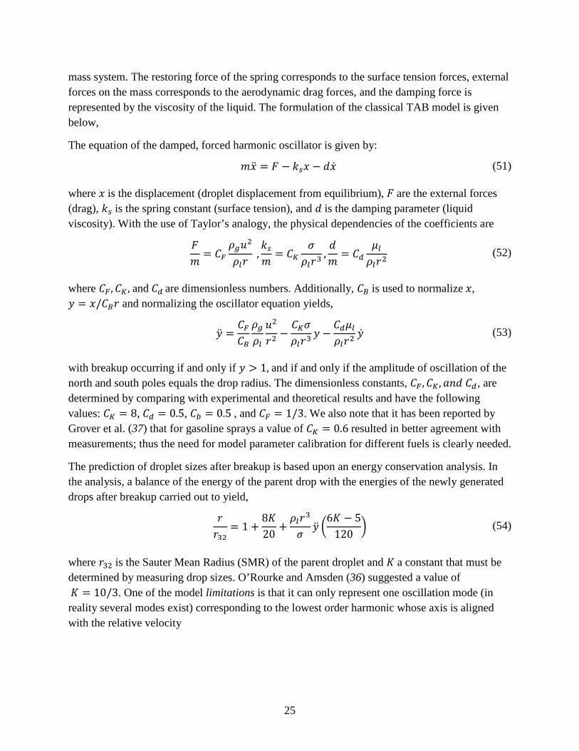
= 𝑒−𝐾𝑏𝑢𝑡 (56) Tanner (38) TAB/E-TAB model performance was validated through a range of conditions representing low-to-intermediate pressure injection into an ambient nonevaporating environment. The breakup constant for the E-TAB were determined through comparison and experimental matching of cross-sectional drop size distribution in the dense region. Figure 12 shows improvements for droplet velocity and droplet size in comparison to the traditional TAB method for an injection time 𝑡𝑖𝑛𝑗 = 1 𝑚𝑠 at 100 nozzle diameters downstream from injection (100𝑑𝑜 = 15 𝑚𝑚).
Figure 12. Drop distribution in the near field fort_inj = 1.0 ms after 100 d downstream (𝑃𝑖𝑛𝑗 = 300 𝑏𝑎𝑟).
27
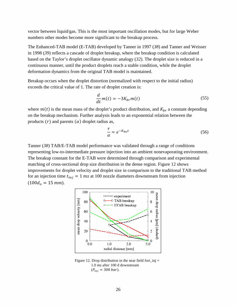
Further model validation is demonstrated with results in good agreement with measurements as shown in figure 13 liquid penetration and the spray angle (radial expansion). Note that a key feature of the TAB models is the ability to compute the radial expansion as part of the calculation.
Figure 13. Comparison of liquid penetration profiles with E-TAB for 3 cases at 𝑃𝑖𝑛𝑗 = 300 𝑏𝑎𝑟. Top case conditions: 𝑃𝑔𝑎𝑠 = 11 𝑏𝑎𝑟 , 𝑡𝑖𝑛𝑗 = 2.5 𝑚𝑠; Middle case: 𝑃𝑔𝑎𝑠 = 30 𝑏𝑎𝑟 , 𝑡𝑖𝑛𝑗 = 4.0 𝑚𝑠 ; Bottom case: 𝑃𝑔𝑎𝑠 = 50 𝑏𝑎𝑟 , 𝑡𝑖𝑛𝑗 = 5.0 𝑚𝑠 .
4.2.5 RT/Hybrid KH-RT/Modified KH-RT Breakup Model
This model is formulated based on theoretical analysis of the stability of liquid-gas interfaces when accelerated in a normal direction to the plane (34). Typically RT instabilities tend to develop when the fluid acceleration has an opposite direction to the density gradient (the interface is stable when acceleration and density gradients are aligned). For a liquid droplet decelerating by drag forces in the gas phase it means that instabilities may grow unstable at the trailing edge of the droplet,
The acceleration of a droplet is due to the drag forces and is mathematically expressed as,
��⃗�� =38𝐶𝐷
𝜌𝑔𝑣𝑟𝑒𝑙2
𝜌𝑙𝑟 (57)
where 𝑣𝑟𝑒𝑙 is the relative velocity between the droplet and gas, 𝑟 is the droplet radius. Assuming a linearized disturbance growth rate and negligible viscosity, the frequency and wavelength of the fastest growing waves are derived as,
ΩRT = �2��⃗��
3���⃗���𝜌𝑙 − 𝜌𝑔�
3𝜎�1/4
(58)
(a) (b)
28
and,
ΛRT = 2𝜋�
3𝜎��⃗���𝜌𝑙 − 𝜌𝑔�
(59)
It is observed that acceleration is the leading term causing a rapid growth of RT instabilities, whereas surface tension counteracts the breakup mechanism.
Traditional (standard) RT models define the growth rate as follows,
𝜔𝑅𝑇 = �𝑘𝑅𝑇 �𝜌𝑙 − 𝜌𝑔𝜌𝑙 + 𝜌𝑔
�𝑎 −𝑘𝑅𝑇3 𝜎𝜌𝑙 + 𝜌𝑔
(60)
More recent efforts have reformulated the growth rate to account for viscosity variations (14),
𝜔𝑅𝑇 = −𝑘𝑅𝑇2 �
𝜇𝑙 + 𝜇𝑔𝜌𝑙 + 𝜌𝑔
� + �𝑘𝑅𝑇 �𝜌𝑙 − 𝜌𝑔𝜌𝑙 + 𝜌𝑔
�𝑎 −𝑘𝑅𝑇3 𝜎𝜌𝑙 + 𝜌𝑔
+ 𝑘𝑅𝑇4 �𝜇𝑙 + 𝜇𝑔𝜌𝑙 + 𝜌𝑔
�2
(61)
The breakup time is found as the reciprocal of the frequency of the fastest growing wave,
𝑡𝑏𝑢 =
1Ω
(62)
The size of the product droplet is calculated based on the RT wavelength Λ , and the breakup process is only allowed when Λ < dparent. Typically the RT model is used in combination of the KH model as a hybrid KH-RT model to describe secondary droplet breakup. In the hybrid case, the RT and KH models are implemented in competing manners, such that the droplet breaks up by the model that predicts a shorter breakup time (40). In the injector nozzle region, where droplet velocities are larger, the RT breakup model dominates, while in KH model is used further downstream.
An additional constraint is enforced, that is used in order to reproduce experimentally intact core or breakup lengths,
𝐿𝑏𝑢 = 𝐶�
𝜌𝑙𝜌𝑔𝑑𝑛𝑜𝑧 (63)
the RT breakup model would predict very rapid breakup directly at the nozzle exit; thus it is switched off within the breakup length provided. Since the RT model predicts the disintegration of a parent droplet into a number of equally sized product droplets, the combination of RT-KH
29
model counteracts the formation of sprays with bimodal droplet size distributions as they would be predicted if the KH model alone is applied as the sole mechanism.
The modified KH-RT model removes the restriction of enforcing a liquid breakup length “a priori.” Primary breakup (of the injected drops) is treated with KH instability model, while secondary breakup is modeled by competing effects of the KH and RT mechanisms (14).
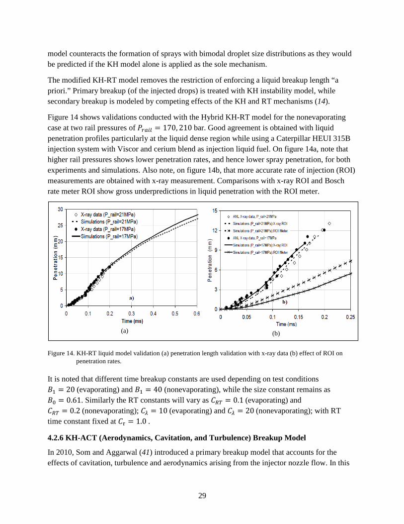
Figure 14 shows validations conducted with the Hybrid KH-RT model for the nonevaporating case at two rail pressures of 𝑃𝑟𝑎𝑖𝑙 = 170, 210 bar. Good agreement is obtained with liquid penetration profiles particularly at the liquid dense region while using a Caterpillar HEUI 315B injection system with Viscor and cerium blend as injection liquid fuel. On figure 14a, note that higher rail pressures shows lower penetration rates, and hence lower spray penetration, for both experiments and simulations. Also note, on figure 14b, that more accurate rate of injection (ROI) measurements are obtained with x-ray measurement. Comparisons with x-ray ROI and Bosch rate meter ROI show gross underpredictions in liquid penetration with the ROI meter.
Figure 14. KH-RT liquid model validation (a) penetration length validation with x-ray data (b) effect of ROI on penetration rates.
It is noted that different time breakup constants are used depending on test conditions 𝐵1 = 20 (evaporating) and 𝐵1 = 40 (nonevaporating), while the size constant remains as 𝐵0 = 0.61. Similarly the RT constants will vary as 𝐶𝑅𝑇 = 0.1 (evaporating) and 𝐶𝑅𝑇 = 0.2 (nonevaporating); 𝐶𝜆 = 10 (evaporating) and 𝐶𝜆 = 20 (nonevaporating); with RT time constant fixed at 𝐶𝜏 = 1.0 .
4.2.6 KH-ACT (Aerodynamics, Cavitation, and Turbulence) Breakup Model
In 2010, Som and Aggarwal (41) introduced a primary breakup model that accounts for the effects of cavitation, turbulence and aerodynamics arising from the injector nozzle flow. In this
(a) (b)
30
study, the effects of the internal turbulent channel flow emanating from the nozzle were reported to be important in predicting a more accurate rate of atomization, liquid penetration depth, and affecting the size of the child droplets.
The model, KH-ACT is quasi-dynamically linked to the inner nozzle flow simulation to provide the cavitation and turbulence transient levels at the nozzle exit as initial and boundary condition conditions as follows.
The turbulence induced breakup model consists of calculating the turbulent time and length scale assuming isotropic internal flow and using the classical decay laws,
𝐿𝑡 = 𝐶𝜇 �
𝐾(𝑡)1.5
𝜖(𝑡) � ; 𝜏𝑡 = 𝐶𝜇 �
𝐾(𝑡)𝜖(𝑡)
�
(64)
where 𝐾(𝑡) and 𝜖(𝑡) are the instantaneous kinetic energy and turbulent dissipation rate, and 𝐶𝜇and 𝐶𝜖 are the model constants. Based on an isotropic turbulence assumption, and neglecting the diffusion, convection, and production terms in the 𝑘 − 𝜖 equation the following estimates are used for 𝐾(𝑡) and 𝜖(𝑡),
𝐾(𝑡) = �
(𝐾0)𝐶𝜖
𝐾0�1 + 𝐶𝜇 − 𝐶𝜇𝐶𝜖� + 𝜖𝑡(𝐶𝜖 − 1)�1/(1−𝐶𝜖)
(65)
𝜖(𝑡) = 𝜖 �
𝐾(𝑡)𝐾0
�𝐶𝜖
(66)
where 𝐾0 and 𝜖0 are the initial values at the nozzle exit at start of injection (SOI), determined from precursor nozzle flow simulations conducted by Som and Aggarwal (41).
The cavitation induced breakup model considers the generation of cavities in the nozzle injector that may travel downstream and reach the nozzle exit; the mechanism of implosion enhances jet atomization process decreasing characteristic breakup timescales. The timescale is set by the faster of two physical mechanisms occurring from the burst of the cavity at the jet periphery or by collapse before reaching it,
𝜏𝐶𝐴𝑉 = 𝑚𝑖𝑛�𝜏𝑐𝑜𝑙𝑙𝑎𝑝𝑠𝑒: 𝜏𝑏𝑢𝑟𝑠𝑡� (67)
The bubble collapse time is calculated from the Rayleigh Plesset theory as the time taken for a bubble of a given radius “r” to decrease to zero,
31
𝜏𝑐𝑜𝑙𝑙𝑎𝑝𝑠𝑒 = 0.9145𝑅𝐶𝐴𝑉�
𝜌𝑙𝑝𝑣
(68)
where 𝑝𝑣 is the fuel vapor pressure, 𝜌𝑙 is the fuel density, and 𝑅𝐶𝐴𝑉 is the effective radius of an equivalent bubble from the nozzle, 𝑅𝐶𝐴𝑉 = 𝑟ℎ𝑜𝑙𝑒�1 − 𝐶𝑎; and the area reduction coefficient 𝐶𝑎 is calculated from precursor internal flow nozzle calculations, and 𝑟ℎ𝑜𝑙𝑒 is the exit radius.
The average time required for a cavitation bubble to reach the periphery of the jet can be estimated as,
𝜏𝑏𝑢𝑟𝑠𝑡 =
𝑟ℎ𝑜𝑙𝑒 − 𝑅𝐶𝐴𝑉𝑢𝑡𝑢𝑟𝑏′ (69)
Where the turbulent velocity 𝑢𝑡𝑢𝑟𝑏′ = �2𝐾(𝑡)/3 is obtained from the precursor calculation; the length scale for the cavitation induced breakup is calculated as 𝐿𝐶𝐴𝑉 = 𝑅𝐶𝐴𝑉 .
Aerodynamically induced breakup model KH model is used to calculate the instantaneous length and timescales for every parcel as,
𝐿𝐾𝐻 = 𝑟 − 𝑟𝐾𝐻 (70)
𝜏𝐾𝐻 =
3.276𝐵1𝑟Ω𝐾𝐻ΛKH
(71)
The ratio of length and timescales for each process is calculated since the largest value will determine the dominant breakup process,
𝐿𝐴𝜏𝐴
= 𝑚𝑎𝑥 �𝐿𝐾𝐻(𝑡)𝜏𝐾𝐻(𝑡)
;𝐿𝐶𝐴𝑉(𝑡)𝜏𝐶𝐴𝑉(𝑡)
;𝐿𝑇(𝑡)𝜏𝑇(𝑡)
� (72)
In the case where aerodynamic induced breakup is dominant, then the previously presented KH model is employed for primary atomization. When cavitation or turbulence are the dominant mechanisms the following breakup law is used,
𝑑𝑟𝑑𝑡
= −𝐶𝑇,𝐶𝐴𝑉 𝐿𝐴𝜏𝐴
(73)
where 𝐶𝑇,𝐶𝐴𝑉 is a model constant.
32
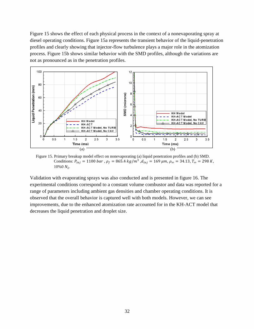
Figure 15 shows the effect of each physical process in the context of a nonevaporating spray at diesel operating conditions. Figure 15a represents the transient behavior of the liquid-penetration profiles and clearly showing that injector-flow turbulence plays a major role in the atomization process. Figure 15b shows similar behavior with the SMD profiles, although the variations are not as pronounced as in the penetration profiles.
Figure 15. Primary breakup model effect on nonevaporating (a) liquid penetration profiles and (b) SMD. Conditions: 𝑃𝑖𝑛𝑗 = 1100 𝑏𝑎𝑟 , 𝜌𝑓 = 865.4 𝑘𝑔/𝑚3 ,𝑑𝑖𝑛𝑗 = 169 𝜇𝑚, 𝜌∞ = 34.13, 𝑇∞ = 298 𝐾, 10%0 𝑁2.
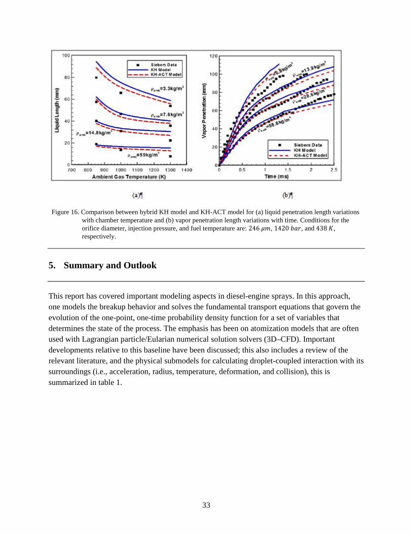
Validation with evaporating sprays was also conducted and is presented in figure 16. The experimental conditions correspond to a constant volume combustor and data was reported for a range of parameters including ambient gas densities and chamber operating conditions. It is observed that the overall behavior is captured well with both models. However, we can see improvements, due to the enhanced atomization rate accounted for in the KH-ACT model that decreases the liquid penetration and droplet size.
(a) (b)
33
Figure 16. Comparison between hybrid KH model and KH-ACT model for (a) liquid penetration length variations with chamber temperature and (b) vapor penetration length variations with time. Conditions for the orifice diameter, injection pressure, and fuel temperature are: 246 𝜇𝑚, 1420 𝑏𝑎𝑟, and 438 𝐾, respectively.
5. Summary and Outlook
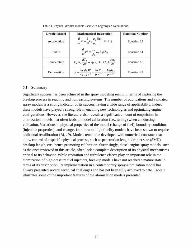
This report has covered important modeling aspects in diesel-engine sprays. In this approach, one models the breakup behavior and solves the fundamental transport equations that govern the evolution of the one-point, one-time probability density function for a set of variables that determines the state of the process. The emphasis has been on atomization models that are often used with Lagrangian particle/Eularian numerical solution solvers (3D–CFD). Important developments relative to this baseline have been discussed; this also includes a review of the relevant literature, and the physical submodels for calculating droplet-coupled interaction with its surroundings (i.e., acceleration, radius, temperature, deformation, and collision), this is summarized in table 1.
34
Table 1. Physical droplet models used with Lagrangian calculations.
Droplet Model Mathematical Description Equation Number
Acceleration 𝑑𝑑𝑡𝐯 =
38𝐶𝑑𝜌𝑔𝜌𝑔
||𝐯𝐫||𝑟
𝐯𝐫 + 𝐠 Equation 13
Radius 𝑑𝑑𝑡𝑟2 =
𝜌𝑣𝜌𝑑𝐷𝑣𝐵𝑑𝑆ℎ𝑑 Equation 14
Temperature 𝐶𝑑𝑚𝑑𝑑𝑇𝑑𝑑𝑡
= 𝑞ℎ𝑆𝑑 + 𝐿(𝑇𝑑)𝑑𝑚𝑑
𝑑𝑡 Equation 18
Deformation �̈� =𝐶𝐹𝐶𝐵𝜌𝑔𝜌𝑙𝑢2
𝑟2−𝐶𝐾𝜎𝜌𝑙𝑟3
𝑦 −𝐶𝑑𝜇𝑙𝜌𝑙𝑟2
�̇� Equation 22
5.1 Summary
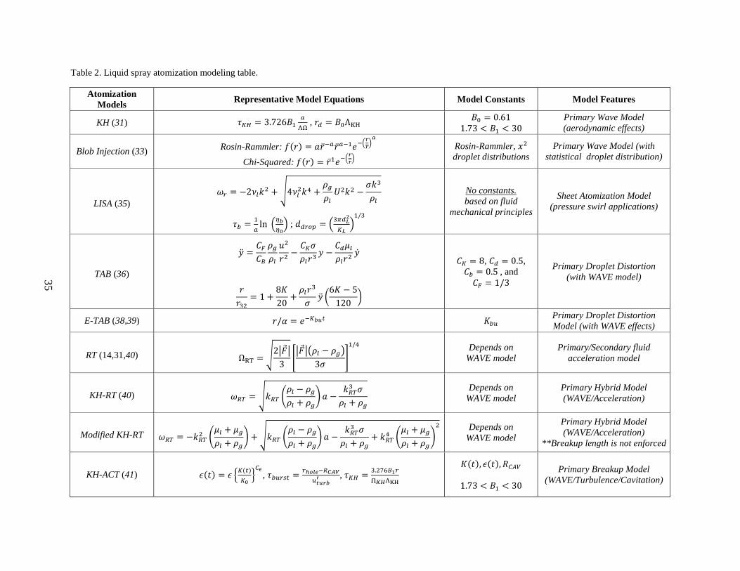
Significant success has been achieved in the spray modeling realm in terms of capturing the breakup process in reacting and nonreacting systems. The number of publications and validated spray models is a strong indicator of its success having a wide range of applicability. Indeed, these models have played a strong role in enabling new technologies and optimizing engine configurations. However, the literature also reveals a significant amount of empiricism in atomization models that often leads to model calibration (i.e., tuning) when conducting validation. Variations in physical properties of the model (change of fuel), boundary conditions (injection properties), and changes from low-to-high fidelity models have been shown to require additional recalibration (18, 19). Models tend to be developed with numerical constants that allow control of a specific physical process, such as penetration length, droplet size (SMD), breakup length, etc., hence promoting calibration. Surprisingly, diesel engine spray models, such as the ones reviewed in this article, often lack a complete description of its physical mechanisms critical to its behavior. While cavitation and turbulence effects play an important role in the atomization of high-pressure fuel injectors, breakup models have not reached a mature state in terms of its description. Its implementation in a contemporary spray-atomization model has always presented several technical challenges and has not been fully achieved to date. Table 2 illustrates some of the important features of the atomization models presented.
35
Table 2. Liquid spray atomization modeling table.
Atomization Models Representative Model Equations Model Constants Model Features
KH (31) 𝜏𝐾𝐻 = 3.726𝐵1𝑎ΛΩ
, 𝑟𝑑 = 𝐵0ΛKH 𝐵0 = 0.61 1.73 < 𝐵1 < 30
Primary Wave Model (aerodynamic effects)
Blob Injection (33) Rosin-Rammler: 𝑓(𝑟) = 𝑎�̅�−𝑎�̅�𝑎−1𝑒−�𝑟𝑟��𝑎
Chi-Squared: 𝑓(𝑟) = �̅�1𝑒−�
𝑟𝑟��
Rosin-Rammler, 𝑥2 droplet distributions
Primary Wave Model (with statistical droplet distribution)
LISA (35) 𝜔𝑟 = −2𝜈𝑙𝑘2 + �4𝜈𝑙2𝑘4 +
𝜌𝑔𝜌𝑙𝑈2𝑘2 −
𝜎𝑘3
𝜌𝑙
𝜏𝑏 = 1𝑎
ln �𝜂𝑏𝜂0� ; 𝑑𝑑𝑟𝑜𝑝 = �3𝜋𝑑𝐿
2
𝐾𝐿�1/3
No constants. based on fluid
mechanical principles
Sheet Atomization Model (pressure swirl applications)
TAB (36)
�̈� =𝐶𝐹𝐶𝐵𝜌𝑔𝜌𝑙𝑢2
𝑟2−𝐶𝐾𝜎𝜌𝑙𝑟3
𝑦 −𝐶𝑑𝜇𝑙𝜌𝑙𝑟2
�̇�
𝑟𝑟32
= 1 +8𝐾20
+𝜌𝑙𝑟3
𝜎�̈� �
6𝐾 − 5120
�
𝐶𝐾 = 8, 𝐶𝑑 = 0.5, 𝐶𝑏 = 0.5 , and 𝐶𝐹 = 1/3
Primary Droplet Distortion (with WAVE model)
E-TAB (38,39) 𝑟/𝛼 = 𝑒−𝐾𝑏𝑢𝑡 𝐾𝑏𝑢 Primary Droplet Distortion Model (with WAVE effects)
RT (14,31,40) ΩRT = �2��⃗��3
���⃗���𝜌𝑙 − 𝜌𝑔�
3𝜎�1/4
Depends on
WAVE model Primary/Secondary fluid
acceleration model
KH-RT (40) 𝜔𝑅𝑇 = �𝑘𝑅𝑇 �𝜌𝑙 − 𝜌𝑔𝜌𝑙 + 𝜌𝑔
� 𝑎 −𝑘𝑅𝑇3 𝜎𝜌𝑙 + 𝜌𝑔
Depends on
WAVE model Primary Hybrid Model (WAVE/Acceleration)
Modified KH-RT 𝜔𝑅𝑇 = −𝑘𝑅𝑇2 �𝜇𝑙 + 𝜇𝑔𝜌𝑙 + 𝜌𝑔
� + �𝑘𝑅𝑇 �𝜌𝑙 − 𝜌𝑔𝜌𝑙 + 𝜌𝑔
� 𝑎 −𝑘𝑅𝑇3 𝜎𝜌𝑙 + 𝜌𝑔
+ 𝑘𝑅𝑇4 �𝜇𝑙 + 𝜇𝑔𝜌𝑙 + 𝜌𝑔
�2
Depends on
WAVE model
Primary Hybrid Model (WAVE/Acceleration)
**Breakup length is not enforced
KH-ACT (41) 𝜖(𝑡) = 𝜖 �𝐾(𝑡)𝐾0�𝐶𝜖
, 𝜏𝑏𝑢𝑟𝑠𝑡 = 𝑟ℎ𝑜𝑙𝑒−𝑅𝐶𝐴𝑉𝑢𝑡𝑢𝑟𝑏′ , 𝜏𝐾𝐻 = 3.276𝐵1𝑟
Ω𝐾𝐻ΛKH
𝐾(𝑡), 𝜖(𝑡),𝑅𝐶𝐴𝑉
1.73 < 𝐵1 < 30
Primary Breakup Model (WAVE/Turbulence/Cavitation)
36
5.2 Unresolved Issues and Directions
Cavitation develops due to pockets of low-static pressure and abrupt changes in the internal nozzle geometry. Turbulence is generated from vapor phase disturbances, internal flow conditions, wall roughness, and any microscale manufacturing imperfections on the surface. Cavitation will increase the liquid velocity at the nozzle exit, and hence will influence the formation and quality of the emerging spray. Improved spray development is believed to lead to a more complete combustion process, lower fuel consumption, and reduced emissions. However, cavitation can decrease the flow efficiency (discharge coefficient) due to its effect on the exiting jet. Also, imploding cavitation bubbles inside the orifice can cause material erosion, thus decreasing the life and performance of the injector (29). This effect has only been directly accounted for in the KH-ACT model developed by Som and Aggarwal (41) and introduced in previous sections. Here an empirical approach was utilized to account for turbulence and cavitation, based on idealized assumptions such as internal isotropic turbulent flow and approximations in cavitation number receiving some success for reacting sprays.
Several numerical studies exist with the intent of modeling the flow inside injector under diesel operating conditions (42–45). Typically several multiphase techniques such as interphase tracking methods, two fluid nozzle flow models, and continuum flow models or homogenous equilibrium models (HEMs) have been utilized to study the effects of cavitation in diesel injector nozzle. Recently in 2013, Payri et al. (42) has achieved significant success in predicting injector quantities for a six orifice microsac nozzle with cylindrical holes, and inclined to cavitation effects using continuum flow models. A similar model was used by Salvador et al. (45) with high-fidelity LES techniques to model cavitation in multihole microsac nozzles. Validation was conducted in terms of mass flow, momentum flux, and effective velocity under real operating conditions with success and the mutual interaction between cavitation and turbulence presented. Flow turbulence and vorticity is reported to affect the appearance of cavitation near the orifice inlet, and once vapor phase is present it will promote the turbulence production since the highest values of vorticity in the nozzle are found at the interphase (45). Several other numerical studies exist using Lagrangian multidimensional CFD models to account for the onset and development of cavitation where good agreement has been reported including higher order diagnostics such as turbulent velocity, which is equally influenced by the inherent unsteadiness from cavitation. It has been concluded that cavitation modeling has reached a stage of maturity at which it can consistently identify many of the effects of nozzle design on cavitation, thus making a significant contribution to nozzle performance and optimization (46, 47).
Recently, several studies invoking the use of DNS methodology have surfaced as a tool to develop next-generation primary models (48–53). Particular attention is given to the lack of theories relating to the determination of the smallest length scale in turbulent liquid gas flows. In several works, the DNS methodology has been utilized to provide new databases and promote the development of an LES formulation of liquid atomization (53) through the use of the ELSA
37
model. In ELSA, a single-phase Eularian approach is used to describe the primary breakup region (54). In the downstream region, where the spray is considered to be diluted enough, the spray is represented through conventional Lagrangian particles and their trajectories and evolutions are tracked. It was reported that this approach needs only two modeling constant, and comprehensive validation is found for the whole set of operating conditions without manipulating the constant values (51, 54). Similar efforts were carried out by Desjardin et al. (50), where he modeled a small portion of the breakup region of a simplified diesel injector. Through the use of advanced numerical techniques, Desjardin was able to show the robustness and accuracy of his approach in modeling atomization. Ning and Reitz (51) extended the operating conditions and conducted a validation study using ELSA of nonvaporizing diesel sprays achieving successful comparison with standard KH-RT breakup models and experimental measurements.
In light of these advancements, atomization models have the opportunity to enhance its modeling features to address its shortcomings. Areas where spray breakup models are expected and recommended to improve are as follows:
• Its ability to accurately describe the entire spray process including the primary breakup “dense” region to the “dilute” region.
• Its ability to capture the effects of injector nozzle turbulence and its mutual interaction with cavitation phenomena.
• Its ability to resolve the flow-field with high resolution as in LES/DNS models, without a-priori requirements of recalibration.
• Its ability to capture variations in fuel physical properties, without a-priori requirements of recalibration, important in studying fuel effects on atomization.
• Its ability to include the effects of needle deformation, as it has been reported that for high-injection pressures, needle deformations can be of the same order than needle lifts.
• Its ability to describe the effects of an electrical field or charge, important for engineering level electrostatic spray applications.
38
6. References
1. Shi, Y.; Ge, H.; Reitz, R. Computational Optimization of Internal Combustion Engines, Springer, 2011.
2. Reitz, R. Directions in Internal Combustion Engine Research. Combustion and Flame 2013.
3. Kweon, C. A Review of Heavy-Fueled Rotary Engine Combustion Technologies; ARL-TR-5546; U.S. Army Research Laboratory: Aberdeen Proving Ground, MD, 2011.
4. Champagne, V.; Dinavahi, S.; Leyman, P. Prediction of Particle Velocity for the Cold Spray Process; ARL-TR-5683; U.S. Army Research Laboratory: Aberdeen Proving Ground, MD, 2011.
5. Waits, C.; Hanrahan, B. Fabrication and Testing of Tapered Electro-spray Nozzles; ARL-TR-6226; U.S. Army Research Laboratory: Aberdeen Proving Ground, MD, 2012.
6. Faeth, G.; Hsiang, L.; Wu, P. Structure and Breakup Properties of Sprays. International Journal of Multiphase Flow 1995.
7. Bardi, M.; Payri, R.; Malbec, L.; Bruneaux, G.; Pickett, L.M.; Manin, J.; Bazyn, T.; Genzale, C.; Engine Combustion Network: Comparison of Spray Development, Vaporization, and Combustion in Different Combustion Vessels. Atomization and Sprays 2012.
8. Pickett, L.; Genzale, C.; Bruneaux, G.; Malbec, L.M.; Hermant, L.; Christiansen, C.; Schramm, J. Comparison of Diesel Spray Combustion in Different High-Temperature, High-Pressure Facilities, SAE paper 10FFL-315, 2010.
9. Pickett, L. Introducing the Engine Combustion Network. International Multidimensional Engine Modeling User's Group Meeting at the SAE Congress, Detroit, MI, April 13, 2008. https://imem.cray.com/2008/agenda-2008.html (accessed May 2014).
10. Bazyn,T.; Martin, G.C.; Spray Combustion Measurements in a Flow-Through High Temperature, High Pressure Chamber. ILASS Americas, 23rd Annual Conference on Liquid Atomization and Spray Systems, Ventura, CA, May, 2011.
11. Meijer, M.; Somers, B.; Johnson, J.; Naber, J.; Lee, S.; Malbec, L.M.; Bruneaux, G.; Pickett, L.M.; Bardi, M.; Payri, R.; Bazyn, T. Engine Combustion Network (ECN): Characterization and Comparison of Boundary Conditions for Different Combustion Vessels. Atomization and Sprays 2012, 22(9), 777–806.
12. Siebers, D. Liquid-Phase Fuel Penetration in Diesel Sprays, SAE Transactions 980809, 1998.
39
13. Weber, J.; Spiekermann, P.; Peters, N. Model Calibration for Spray Penetration and Mixture Formation in a High Pressure Fuel Spray Using a Micro-Genetic Algorithm and Optical Data, SAE transactions 2005-01-2099, 2005.
14. Senecal, P.; Richards, K.; Pomraning, E.; Yang, T. A New Parallel Cut-Cell Cartesian CFD Code for Rapid Grid Generation Applied to in-Cylinder Diesel Engine Simulations, SAE 2007-01-0159, 2007.
15. Amsden, T. D.; O’Rourke, A. A.; Butler, P. J. KIVA-II: A Computer Program for Chemically Reactive Flows With Sprays, LA-11560-MS, 1989.
16. Vijayraghavan Iyengar, S.; Tsang, C.; Rutland, C. Validating Non-Reacting Spray Cases With KIVA-3V and OpenFoam, SAE technical paper 2013-01-1595, 2013.
17. Senecal, P.; Pomraning, E.; Richards, K.; Som, S. Grid-Convergent Spray Models for Internal Combustion Engine CFD Simulations. In Proceedings of the ASME 2012 Internal Combustion Engine Division Fall Technical Conference (ICEF2012-92043), 2012.
18. Xue, E. P. Q.; Som, S.; Senecal, P. K. A Study of Grid Resolution and SGS Models for LES Under Non-Reacting Spray Conditions. ILASS Americas, 25th Annual Conference on Liquid Atomization and Spray Systems, Pittsburgh, PA, May 2013.
19. Senecal, P.; Pomraning, E.; Xue, Q.; Som, S. Large Eddy Simulation of Vaporizing Sprays Considering Multi-Injection Averaging and Grid-Convergent Mesh Resolution. Proceedings of the ASME 2013 Internal Combustion Engine Division Fall Technical Conference (ICEF2013-19082), 2013.
20. Habchi, C.; Bruneaux, G. LES and Experimental Investigation of Diesel Sprays. ICLASS 2012, 12th Triennial International Conference on Liquid Atomization and Spray Systems, 2012.
21. Stiesch, G. Modeling Engine Spray and Combustion Processes, Springer, 2003.
22. Lin, S. P.; Reitz, R. D. Drop and Spray Formation From a Liquid Jet. Annual Review of Fluid Mechanics January 1998, 30 (1), 85–105.
23. Reitz, R. D. Mechanisms of Breakup of Round Liquid Jets, Ph. D. thesis, Princeton University, 1978.
24. Ashgriz, N. Handbook of Atomization and Sprays: Theory and Applications; Springer, 2011.
25. Marmottant, P.; Villermaux, E. On Spray Formation. Journal of Fluid Mechanics 2004.
26. Archambault, M. Stochastic Spray Flow Models: A Review, ILASS-Americas 22nd Annual Conference on Liquid Atomization and Spray Systems, Cincinnati, OH, May 2010.
40
27. Pai, G. M.; Subramaniam, S. Accurate Numerical Solution of The Spray Equation Using Particle Methods. Atomization and Sprays 2006, 16 (2), 159–194.
28. Williams, F. Spray Combustion and Atomization. Physics of Fluids 1958.
29. Ashgriz, N. Handbook of Atomization and Sprays: Theory and Applications, Springer, 2011.
30. Schmidt, D.; Rutland, C. A New Droplet Collision Algorithm. Journal of Computational Physics, vol 164, 62-80 2000.
31. Reitz, R.; Diwakar, R. Effect of Drop Breakup on Fuel Sprays, SAE Technical Paper 860469, 1986.
32. Reitz, R. Computer Modeling of Sprays. Spray Technology Short Course, Pittsburgh, PA, 1996.
33. Reitz, R.; Diwakar, R. Structure of High-Pressure Fuel Sprays. SAE Int.J.Engines 870598, 1987.
34. Hwang, S. S.; Liu, Z.; Reitz, R. D. Breakup Mechanisms and Drag Coefficients of High-Speed Vaporizing Liquid Drops. Atomization and Sprays 1996, 6 (3).
35. Senecal, P.; Schmidt, D.; Nouar, I.; Rutland, C.; Reitz, R.; Corradini, M. Modeling High-Speed Viscous Liquid Sheet Atomization. International Journal of Multiphase Flow 1999, 25 (6), 1073–1097.
36. O’Rourke, A.; Amsden, P. The Tab Method for Numerical Calculation of Spray Droplet Breakup. SAE Technical Paper 872089, 1987.
37. Grover, R.O.; Assanis, D.N.; Lippert, A.M.; El Tahry, S.H.; Drake, M.C.; Fansler, T.D.; Harrington, D.L.; A Critical Analysis of Splash Criteria for GDI Spray Impingement, ILASS Americas,15th Annual Conference on Liquid Atomization and Spray Systems, Madison, WI, May 2002.
38. Tanner, F. Liquid Jet Atomization and Droplet Breakup Modeling of Non-Evaporating Diesel Fuel Sprays. SAE Technical Paper 970050, 1997.
39. Tanner, G.; Weisser, F. Simulation of Liquid Jet Atomization for Fuel Sprays by Means of a Cascade Drop Breakup Model, SAE Technical Paper 980808, 1998.
40. Beale, J. Modeling Fuel Injection Using Kelvin-Helmholtz/Rayleigh-Taylor Hybrid Atomization Model In Kiva-3v, M.S. Thesis in Mechanical Engineering, University of Wisconsin, Madison, 1999.
41. Som, S.; Aggarwal, S. K. Effects of Primary Breakup Modeling on Spray and Combustion Characteristics of Compression Ignition Engines. Combustion and Flame June 2010, 157 (6), 1179–1193.
41
42. Payri, F.; Payri, R.; Salvador, F. J.; Martínez-López, J. A Contribution to the Understanding of Cavitation Effects in Diesel Injector Nozzles Through a Combined Experimental and Computational Investigation. Computers & Fluids. 2012, 58, 88–101.
43. Salvador, F. J.; Romero, J.-V.; Roselló, M.-D.; Martinez-Lopez, J. Validation of a Code for Modeling Cavitation Phenomena in Diesel Injector Nozzles. Mathematical and Computer Modelling 2010, 52 (7), 1123–1132.
44. Salvador, F. J.; Martinez-Lopez, J.; Romero, J.-V.; Roselló, M.-D. Influence of Biofuels on the Internal Flow in Diesel Injector Nozzles. Mathematical and Computer Modelling 2011, 54, (7), 1699–1705.
45. Salvador, F. J.; Martinez-Lopez, J.; Romero, J.-V.; Roselló, M.-D. Computational Study of the Cavitation Phenomenon and its Interaction With the Turbulence Developed in Diesel Injector Nozzles by Large Eddy Simulation (LES). Mathematical and Computer Modelling 2013, 57 (7), 1656–1662.
46. Andriotis, A.; Gavaises, M.; Arcoumanis, C. Vortex Flow and Cavitation in Diesel Injector Nozzles. Journal of Fluid Mechanics 2008, 610, 195–215.
47. Giannadakis, E.; Gavaises, M.; Arcoumanis, C. Modelling of Cavitation in Diesel Injector Nozzles. Journal of Fluid Mechanics 2008, 616, 153.
48. Menard, T.; Beau, P.A.; Tanguy, S.; Demoulin, F.X.; Berlemont, A. Primary Breakup Modeling Part A: DNS, A Tool to Explore Primary Breakup. International Conference for Liquid Atomization and Sprays Systems, ICLASS06-034, Kyoto, Japan, 2006.
49. Beau, P.A.; Menard, T.; Lebas, R.; Berlemont, A.; Demoulin, F.-X. Primary Break Up Modeling Part B: Extracting Modeling Information From DNS Based Results. International Conference for Liquid Atomization and Sprays Systems, ICLASS06-037, Kyoto, Japan, 2006.
50. Desjardins, O.; M. H. and H. P., Moureau, V.; Knudsen, E. Conservative Level Set/Ghost Fluid Method for Simulating Primary Atomization. In ILASS Americas 20th Annual Conference on Liquid Atomization and Spray Systems, Chicago, IL, May 2007.
51. Ning, R.; Reitz, W.; Lippert, A.M.; Diwakar, R. Development of a Next-Generation Spray and Atomization Model Using an Eulerian Lagrangian Methodology. In 17th International Multidimensional Engine Modeling User’s Group Meeting, Detroit, Michigan, April 2007.
52. Gorokhovski, M.; Herrmann, M. Modeling Primary Atomization. Annual Review of Fluid Mechanics 2008, 40 (1), 343–366.
53. Demoulin, F. X.; Reveillon, J.; Duret, B.; Bouali, Z.; Desjonqueres, P.; Menard, T. Toward using Direct Numerical Simulation to Improve Primary Break-Up Modeling. Atomization and Sprays 2013.
42
54. Lebas, F.; Blokkeel, R.; Beau, G.; Demoulin, P. Coupling Vaporization Model With the Eulerian-Lagrangian Spray Atomization (ELSA) Model in Diesel Engine Conditions, 2005-01-0213 Technical Paper SAE, 2005.
43
List of Symbols, Abbreviations, and Acronyms
AMR adaptive-mesh-refinement
ARL U.S. Army Research Laboratory
CERFACS Centre Européen de Recherche et de Formation Avancée en Calcul Scientifique
CFD computational fluid dynamics
CPF Constant-Pressure Flow
CVP Constant-Volume Preburn
DNS Direct Numerical Simulation
ECN Engine Combustion Network
EGR exhaust-gas recirculation
ELSA Eularian Lagrangian Spray Atomization
E-TAB Enhanced-TAB model
HEM homogenous equilibrium models
IFPEN French Petroleum Institute
KH Kelvin Helmholtz
LES Large-eddy simulation
LISA Linearized Instability Sheet Atomization
MTU Michigan Technological University
NTC No Time Counter
RANS Reynolds Average Navier Stokes
ROI rate of injection
RT Rayleigh Taylor
SMD Sauter Mean Diameter
SMR Sauter Mean Radius
SNL Sandia National Laboratories
44
SOI start of injection
TAB Taylor Analogy Breakup
TU/e Eindhoven University of Technology
45
1 DEFENSE TECHNICAL
(PDF) INFORMATION CTR
DTIC OCA
2 DIR USARL
(PDF) IMAL HRA
RDRL CIO LL
1 GOVT PRINTG OFC
(PDF) A MALHOTRA
1 DIR USARL
(PDF) RDRL VTP
L BRAVO

46
INTENTIONALLY LEFT BLANK.