Embed Size (px)
Citation preview
INTERNATIONAL JOURNAL OF ROBUST AND NONLINEAR CONTROLInt. J. Robust Nonlinear Control 2009; 19:92–116Published online 22 July 2008 in Wiley InterScience (www.interscience.wiley.com). DOI: 10.1002/rnc.1340
Linear parameter varying control of wind turbines covering bothpartial load and full load conditions
Kasper Zinck Østergaard1,∗,†, Jakob Stoustrup2 and Per Brath1
1Turbine Control and Operation R&D, Vestas Wind Systems A/S, Alsvej 21, 8900 Randers, Denmark2Automation and Control, Department of Electronic Systems, Aalborg University,
Fredrik Bajers Vej 7C, 9220 Aalborg Ø, Denmark
SUMMARY
This paper considers the design of linear parameter varying (LPV) controllers for wind turbines in orderto obtain a multivariable control law that covers the entire nominal operating trajectory.
The paper first presents a controller structure for selecting a proper operating trajectory as a functionof estimated wind speed. The dynamic control law is based on LPV controller synthesis with generalparameter dependency by gridding the parameter space.
The controller construction can, for medium- to large-scale systems, be difficult from a numericalpoint of view, because the involved matrix operations tend to be ill-conditioned. The paper proposes acontroller construction algorithm together with various remedies for improving the numerical conditioningthe algorithm.
The proposed algorithm is applied to the design of a LPV controller for wind turbines, and a compar-ison is made with a controller designed using classical techniques to conclude that an improvement inperformance is obtained for the entire operating envelope. Copyright q 2008 John Wiley & Sons, Ltd.
Received 1 August 2007; Revised 4 April 2008; Accepted 7 April 2008
KEY WORDS: linear parameter varying control; control of wind turbines; gain scheduling; numericalconditioning
1. INTRODUCTION
In the wind energy industry, there has been a large focus on increasing the capacity of wind turbinesin order to reduce the installation costs when compared with the power production during thelifetime of the wind turbine. This has resulted in a rapid growth in rotor size and electrical powerproduction, and in the period from 1980 to 2003 the largest wind turbine size has grown fromapproximately 50 to 5000 kW,which is more than a 20% increase per year for more than 20 years [1].
∗Correspondence to: Kasper Zinck Østergaard, Turbine Control and Operation R&D, Vestas Wind Systems A/S,Alsvej 21, 8900 Randers, Denmark.
†E-mail: [email protected]
Copyright q 2008 John Wiley & Sons, Ltd.
LINEAR PARAMETER VARYING CONTROL OF WIND TURBINES 93
This dramatic increase in wind turbine size and capacity has made it very challenging to designwind turbines, because many of the structural and electrical components are not scalable, i.e. thecosts introduced by scaling the components grow at a higher rate than the benefits from increasedproduction. For the structural components, this means that the components must be made lighterwithout compromising their durability, e.g. by improving the performance of active control.
Previous investigations such as [2–6] have shown that linear, time-invariant methods providegood closed-loop results when observing local behaviour. A natural choice for controller designcovering the entire operating envelope is therefore to design linear controllers along a chosenoperating trajectory and then to interconnect them in an appropriate way in order to get a controlformulation for the entire operating region. This approach is denoted as gain scheduling andin [7–9] this is done by interpolating the outputs of a set of local controllers (either by linearinterpolation or by switching). Alternatively, parameters of the controller are updated according toa pre-specified function of a measured/estimated variable [10–12].
A systematic way of designing such parameter-dependent controllers is within the frameworkof linear parameter varying (LPV) systems. Here, the model will be represented by a linear modelat all operating conditions and a controller with similar parameter dependency is synthesized toguarantee a certain performance specification for all possible parameter values within a specifiedset. A major difference to classical gain scheduling is that it is possible to take into account thatthe scheduling parameters can vary in time. In this paper we will, due to numerical considerations,assume arbitrary fast parameter variations, which is the most restrictive form of LPV control.
In [13–15] the LPV design procedure is applied for the special case of affine parameter depen-dency. However, affine parameter dependency is a very strict requirement for designing controllersfor wind turbines in the entire operating region. Mainly because the performance criteria are verydifferent in partial load when compared with full load control, but also because it is rather crude toapproximate the nonlinear aerodynamics by a first-order function over the entire operating region.In [13, 14] this is handled by designing different LPV controllers for the below- and above-ratedwind speeds and then switching between them.
The gain-scheduled design methods in the literature consider one controller for partial loadand another controller for full load operation (except for [15] in which a simplistic parameterdependency is assumed). This means that a method for bumpless transfer between two very differentcontrollers needs to be implemented to make the control law work in practice. In this paper weconsider an alternative approach in which a gain-scheduled controller is designed for both partialload and full load operations for a 3MW wind turbine with a rotor diameter of 90m.
As performance criteria, the design will focus on tracking a generator speed reference togetherwith minimization of fatigue damage in vital components, e.g. drive train and tower. Controleffort is also taken into account to avoid the pitch system to wear out and the power fluctuationsto be too high. In order to handle the very different performance criteria for low wind speedsand high wind speeds, it has been decided to use a grid-based method as in [16], because itmakes it possible to use a general form of parameter dependency. The controller construction isvery sensitive to numerical issues and a number of remedies are presented for conditioning theconstruction procedure. To reduce numerical complexity, it has been decided to focus only onarbitrary fast parameter variations throughout the paper.
The paper is structured as follows. In Section 2 we discuss the closed-loop objectives that will beconsidered in the design process and in Section 3 the considered wind turbine model is presented.A controller structure is given in Section 4 for tracking the desired target trajectory. This sectionis followed by a presentation of the performance channel for the LPV design in Section 5. Then in
Copyright q 2008 John Wiley & Sons, Ltd. Int. J. Robust Nonlinear Control 2009; 19:92–116DOI: 10.1002/rnc
94 K. Z. ØSTERGAARD, J. STOUSTRUP AND P. BRATH
Section 6 the LPV controller design method is presented and a discussion of numerical remediesfor controller construction is made in Section 7. In Section 8 closed-loop simulation results arepresented and conclusions are given in Section 9.
2. CONTROL OBJECTIVES
The main objective for wind turbine controllers is to maximize the trade-off between the annualenergy production and the construction and maintenance costs of the wind turbine. This has resultedin two operational modes for pitch-regulated variable-speed wind turbines: partial load and fullload operations.
Partial load operation is the mode in which there is not enough kinetic energy in the wind toachieve nominal electrical power production. In this mode the primary objective is to control thepitch and rotor speed to achieve the maximum aerodynamic efficiency of the wind turbine.
Full load operation is the mode in which the kinetic energy in the wind field has exceeded thenominal electrical power production and conversion losses. In this mode the generator speed shouldbe kept close to the nominal speed and the pitch angle should be controlled to achieve nominalelectrical power production. Further, it is important to reduce the fluctuations on the power, knownas flicker.
In both operating regions, it is important to minimize the fatigue loads in critical structuralcomponents, and in this paper the following three components will be considered: drive train,tower in the fore–aft direction, and pitch system.
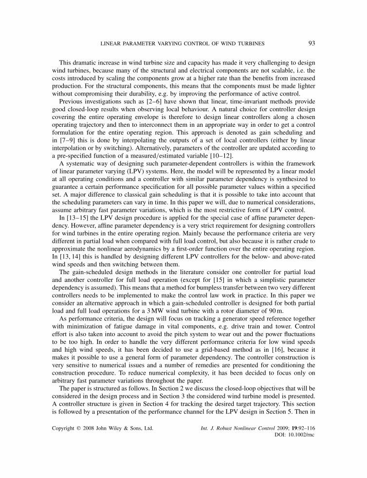
In addition, it is crucial that the generator speed does not exceed the maximum generator speed inorder not to overheat the electrical components. When combining these conditions, the steady-statetrajectory of the wind turbine can be described by a function of wind speed, which is illustratedin Figure 1. The requirements regarding optimization of power production and deviations fromnominal generator speed then amount to tracking the steady-state trajectory in Figure 1 as closelyas possible.
The other performance criteria can be seen as detuning of the tracking controller to limitstructural oscillations and high amounts of control effort. For the pitch activity, it is well knownthat during high wind speeds a high amount of activity is required to track the target trajectory andminimize tower loads. During low wind speeds, the pitch angle should be kept close to the valueyielding maximum aerodynamic performance. This means that there needs to be a high emphasison the wear in the pitch system during low wind speeds, whereas higher variations can be toleratedduring high wind speeds.
10 20
0
10
20
wind speed [m/s]
pitc
h an
gle
[deg
]
10 2010
12
14
16
wind speed [m/s]
roto
r sp
eed
[rpm
]
10 200
1
2
3
wind speed [m/s]
pow
er [M
W]
Figure 1. Illustration of operating region for wind turbine.
Copyright q 2008 John Wiley & Sons, Ltd. Int. J. Robust Nonlinear Control 2009; 19:92–116DOI: 10.1002/rnc
LINEAR PARAMETER VARYING CONTROL OF WIND TURBINES 95
As discussed above, the requirements are different for low wind speeds and high wind speeds.This is not only in terms of use of the control signals, but also for fatigue loads and trackingperformance because the energy in the wind increases with wind speed. Since the wind speedwill vary between low wind speeds and high wind speeds, the performance criteria will changesignificantly during operation. In the sequel, we shall demonstrate that a systematic approach toobtain the above objectives can be achieved by the virtue of an LPV controller design. In thismanner we obtain a smooth transition between controllers satisfying the design requirements alongthe design trajectory. Further, it shall be noted that nonlinearities caused, for example, by theaerodynamics can easily be incorporated into the LPV design framework.
3. WIND TURBINE MODEL
Based on the control objectives presented in the previous section, a nonlinear model of suitablecomplexity will be constructed. Then in order to obtain an LPV model, the nonlinear model islinearized along the desired operating trajectory.
It has been evaluated that five components have to be modelled in order to perform a propercontroller design according to the presented requirements: drive train, tower, aerodynamics, pitchsystem, and generator and converter system. These five components will be presented in thefollowing sections.
3.1. Drive train
The drive train is modelled by two inertias interconnected by a spring and a damper. In this design,the dynamics of the blades will not be included, and the blade stiffness and inertia are thereforelumped into the slow-speed shaft. Friction is included in terms of linear friction coefficients oneach shaft. This leads to the following formulation of the drive train model:
Jr�r = Qa−Br�r−N�(N�r−�g)−NK�� (1a)
Jg�g = −Qg−Bg�g+�(N�r−�g)+K�� (1b)
�� = N�r−�g (1c)
Qsh = �(N�r−�g)+K�� (1d)
where �r and �g are the rotational speeds of, respectively, the slow- and high-speed shaft, �� is theangular difference between slow- and high-speed shaft, Qa and Qg are, respectively, aerodynamictorque and generator reaction torque, Jr and Jg are the two moments of inertia, Br and Bg arethe friction coefficients on the two shafts, N is the gearing ratio, K and � are the stiffness anddamping coefficients of the interconnection of the two inertias, and Qsh is the torque between thetwo shafts.
3.2. Tower
The tower will be modelled by a mass–spring system as in (2) with pt as the displacement of thetower top, m is the equivalent mass, Bt is the structural damping of the tower, Kt is the towerstiffness, and Ft is the thrust on the tower
m pt=Ft−Bt pt−Kt pt (2)
Copyright q 2008 John Wiley & Sons, Ltd. Int. J. Robust Nonlinear Control 2009; 19:92–116DOI: 10.1002/rnc
96 K. Z. ØSTERGAARD, J. STOUSTRUP AND P. BRATH
Aerodynamic efficiency, cP
tip speed ratio [ ]
pitc
h an
gle
[deg
]
5 10 15 20
0
10
20
30
40
Aerodynamic efficiency, c T
tip speed ratio [ ]
pitc
h an
gle
[deg
]
5 10 15 20
0
10
20
30
40
Figure 2. Illustration of aerodynamic efficiency and thrust coefficient. Light shades indicate smallcoefficients and dark shades indicate large coefficients.
3.3. Aerodynamics
The aerodynamics will be approximated by static functions of spatial average of wind speed, rotorspeed, and pitch angle according to [17]
Qa = 1
2��R2 v3
�rcP(�,�) (3a)
Ft = 12��R2v2cT (�,�) (3b)
� = �rR
v(3c)
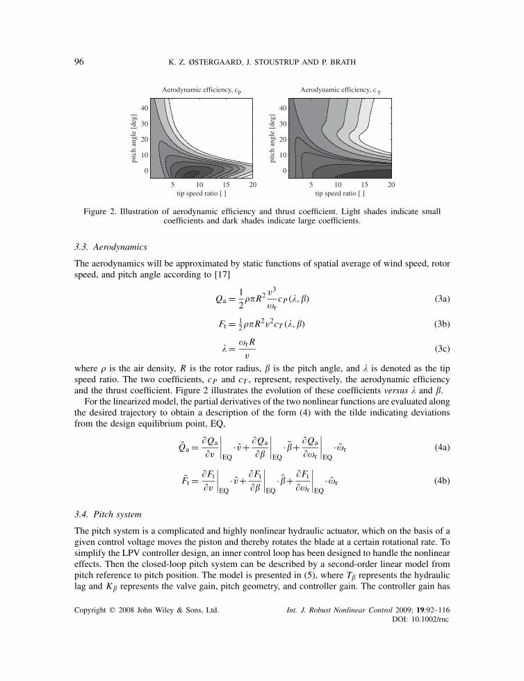
where � is the air density, R is the rotor radius, � is the pitch angle, and � is denoted as the tipspeed ratio. The two coefficients, cP and cT , represent, respectively, the aerodynamic efficiencyand the thrust coefficient. Figure 2 illustrates the evolution of these coefficients versus � and �.
For the linearized model, the partial derivatives of the two nonlinear functions are evaluated alongthe desired trajectory to obtain a description of the form (4) with the tilde indicating deviationsfrom the design equilibrium point, EQ,
Qa = �Qa
�v
∣∣∣∣EQ
· v+ �Qa
��
∣∣∣∣EQ
· �+ �Qa
��r
∣∣∣∣EQ
·�r (4a)
Ft = �Ft�v
∣∣∣∣EQ
· v+ �Ft��
∣∣∣∣EQ
· �+ �Ft��r
∣∣∣∣EQ
·�r (4b)
3.4. Pitch system
The pitch system is a complicated and highly nonlinear hydraulic actuator, which on the basis of agiven control voltage moves the piston and thereby rotates the blade at a certain rotational rate. Tosimplify the LPV controller design, an inner control loop has been designed to handle the nonlineareffects. Then the closed-loop pitch system can be described by a second-order linear model frompitch reference to pitch position. The model is presented in (5), where T� represents the hydrauliclag and K� represents the valve gain, pitch geometry, and controller gain. The controller gain has
Copyright q 2008 John Wiley & Sons, Ltd. Int. J. Robust Nonlinear Control 2009; 19:92–116DOI: 10.1002/rnc
LINEAR PARAMETER VARYING CONTROL OF WIND TURBINES 97
–50
0
50
ωg
V Qg,ref βref
–100
–50
0
50Q
sh
10 –1
100
101
102
–100
– 50
0
p t,vel
Freq [rad/s]10
– 110
010
110
2
Freq [rad/s]10
–110
010
110
2
Freq [rad/s]
vv
v
vv
v
v
v
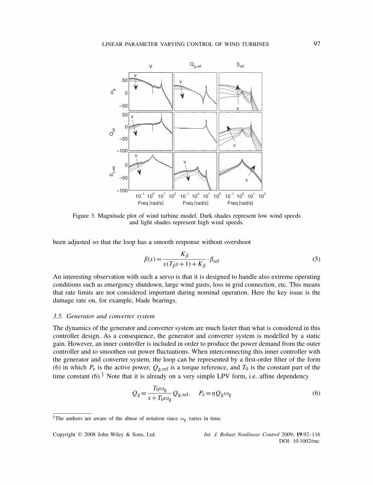
Figure 3. Magnitude plot of wind turbine model. Dark shades represent low wind speedsand light shades represent high wind speeds.
been adjusted so that the loop has a smooth response without overshoot
�(s)= K�
s(T�s+1)+K�·�ref (5)
An interesting observation with such a servo is that it is designed to handle also extreme operatingconditions such as emergency shutdown, large wind gusts, loss in grid connection, etc. This meansthat rate limits are not considered important during nominal operation. Here the key issue is thedamage rate on, for example, blade bearings.
3.5. Generator and converter system
The dynamics of the generator and converter system are much faster than what is considered in thiscontroller design. As a consequence, the generator and converter system is modelled by a staticgain. However, an inner controller is included in order to produce the power demand from the outercontroller and to smoothen out power fluctuations. When interconnecting this inner controller withthe generator and converter system, the loop can be represented by a first-order filter of the form(6) in which Pe is the active power, Qg,ref is a torque reference, and T0 is the constant part of thetime constant (6).‡ Note that it is already on a very simple LPV form, i.e. affine dependency
Qg= T0�g
s+T0�gQg,ref, Pe=�Qg�g (6)
‡The authors are aware of the abuse of notation since �g varies in time.
Copyright q 2008 John Wiley & Sons, Ltd. Int. J. Robust Nonlinear Control 2009; 19:92–116DOI: 10.1002/rnc
98 K. Z. ØSTERGAARD, J. STOUSTRUP AND P. BRATH
3.6. Interconnection
With the above-described components, the wind turbine model can be obtained by the standardinterconnection of the blocks described in the above sections. The only nonlinear componentsdescribed above are the aerodynamics and generator system. With the assumption that the windturbine is operating on the nominal trajectory specified in Figure 1, the equilibrium values forpitch angle and rotor/generator speed can be described uniquely by the wind speed. This meansthat the wind turbine model can be described by an LPV model scheduled on only wind speed asillustrated in Figure 3.
4. CONTROLLER STRUCTURE
Before discussing the specific choice of the controller structure, it is important to understand thedesired behaviour of the control system in the different operating modes. In partial load operation,an important objective is to maximize the electrical power production. This means that the pitchangle and rotor speed should be controlled in a way so that the aerodynamic coefficient, cP , ismaximized. By observing the leftmost illustration in Figure 2, it implies that the pitch angle shouldbe kept constant close to −2◦ and the rotor speed should be controlled proportional to the effectivewind speed to get an optimal tip speed ratio. In practice, this will be done by tracking a generatorspeed reference via an update of the generator torque.
In full load operation, the generator speed and power needs to be kept close to constant nominalvalues, which means that the generator torque should be varied as little as possible. The pitchposition as the remaining control signal is controlled to keep the aerodynamic power constantthereby keeping the electric power constant.
The main part of the controller structure is then a set-up for tracking a specified generator speedreference by mainly using generator torque in partial load operation and pitch angle in full loadoperation. On top of this main structure, there will be components using both control signals inorder to minimize the oscillations in drive train and tower fore–aft movement. For the minimizationof tower oscillations a measurement of tower acceleration is included.
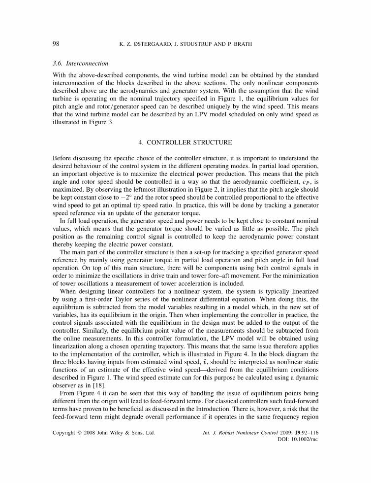
When designing linear controllers for a nonlinear system, the system is typically linearizedby using a first-order Taylor series of the nonlinear differential equation. When doing this, theequilibrium is subtracted from the model variables resulting in a model which, in the new set ofvariables, has its equilibrium in the origin. Then when implementing the controller in practice, thecontrol signals associated with the equilibrium in the design must be added to the output of thecontroller. Similarly, the equilibrium point value of the measurements should be subtracted fromthe online measurements. In this controller formulation, the LPV model will be obtained usinglinearization along a chosen operating trajectory. This means that the same issue therefore appliesto the implementation of the controller, which is illustrated in Figure 4. In the block diagram thethree blocks having inputs from estimated wind speed, v, should be interpreted as nonlinear staticfunctions of an estimate of the effective wind speed—derived from the equilibrium conditionsdescribed in Figure 1. The wind speed estimate can for this purpose be calculated using a dynamicobserver as in [18].
From Figure 4 it can be seen that this way of handling the issue of equilibrium points beingdifferent from the origin will lead to feed-forward terms. For classical controllers such feed-forwardterms have proven to be beneficial as discussed in the Introduction. There is, however, a risk that thefeed-forward term might degrade overall performance if it operates in the same frequency region
Copyright q 2008 John Wiley & Sons, Ltd. Int. J. Robust Nonlinear Control 2009; 19:92–116DOI: 10.1002/rnc
LINEAR PARAMETER VARYING CONTROL OF WIND TURBINES 99
Figure 4. Implementation structure for an LPV controller based on linearizationalong a trajectory of equilibrium points.
as the LPV controller. In this case it should be included in the LPV design using a two degrees-of-freedom controller design, e.g. along the lines of [19]. It is expected that the feed-forward termswill not interfere with the LPV controller because of the successful results obtained for classicalcontrollers. The LPV design presented in this paper will, therefore, not include feed-forward terms,because this would increase the dimensionality of the design problem and thereby make numericaldifficulties more likely.
5. SELECTION OF PERFORMANCE CHANNELS AND ASSOCIATED WEIGHTS
In the applied formulation of LPV control, the performance is measured in terms of energyamplification from a number of selected inputs to a selection of outputs—very similar to H∞control. However, the objectives in Section 2 are given in physical terms, such as to minimize thefatigue damage in the tower, to limit the maximum generator speed, etc. As performance input,the wind speed is chosen and to transform the objectives into something that can be measured byenergy amplification, the following performance outputs have been chosen.
Tower top velocity in the fore–aft direction, y: The tower is lightly damped close to its eigen-frequency and it is therefore most important to actively dampen oscillations around this frequency.In the linearized model, the bode diagram of the transfer function from wind speed to tower topvelocity has a peak at the tower eigenfrequency—along the entire operating trajectory. Thus, byintroducing a frequency-independent scaling of this performance output, the dampening of theoscillations around the tower eigenfrequency can be included in the performance function forcontroller design.
Torsion torque in drive train, Qsh: For the drive train the issue is very similar, because it islightly damped around its eigenfrequency. The bode diagram of the transfer function from windspeed to shaft torque has a peak at this eigenfrequency, which means that a frequency-independentscaling can be used—with the same argumentation as for the tower.
Tracking error for generator speed, �e: The main target of using this performance output isto minimize the variations in generator speed, from the design trajectory, caused by variationsin wind speed. The main content of the wind speed is in lower frequencies, which means thatputting an emphasis on low-frequency components will be satisfactory. Because the low-frequencycomponents are dominant in the transfer function from wind speed to generator speed (for all thelinearized models) this means that again a frequency-independent scaling is applicable. However,the scaling should be gain scheduled by effective wind speed to take into account that the issue of
Copyright q 2008 John Wiley & Sons, Ltd. Int. J. Robust Nonlinear Control 2009; 19:92–116DOI: 10.1002/rnc
100 K. Z. ØSTERGAARD, J. STOUSTRUP AND P. BRATH
overspeeds is most likely to occur around rated generator speed, i.e. a larger weight for mediumwind speeds than on high and low wind speeds should be used.
Pitch activity, �: It is very undesirable to have high-frequency content in the controlled pitchangle because this would cause a high amount of wear in blade bearings and in the pitch hydraulics.In partial load operation, there is a very limited control authority in the pitch actuator because thewind turbine is operating close to aerodynamic optimality. As a consequence, the generator torqueis the main control signal in low wind speeds and it is cheap to limit pitch activity in this region.At high wind speeds, the pitch system is the main actuator and limiting the pitch activity has amuch higher impact on the other structural loads. It has therefore been decided to gain schedulethe weight on pitch activity to allow for high activity in full load operation and low activity inpartial load operation. Further, the weight will be in the form of a high pass filter to make thehigh-frequency pitch activity more expensive than the low-frequency activity.
Variations in generator torque, Qg: In the linearized model for controller design, the electricalpower is not directly accessible as a linear combination of states and inputs. In full load operation,where the steady-state generator speed is constant, the variations in generator torque relate ina direct way to power fluctuations. Therefore, the generator torque will be weighted by a largefrequency-independent scaling at high wind speeds, whereas a smaller scaling is used for low windspeeds to allow for sufficient tracking of generator speed reference.
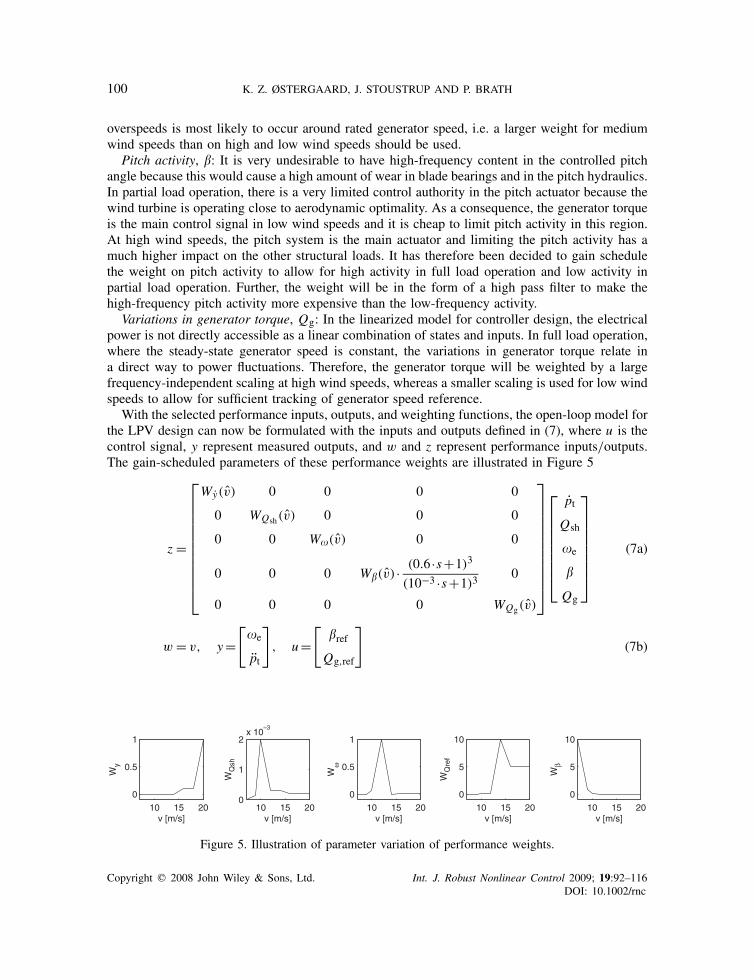
With the selected performance inputs, outputs, and weighting functions, the open-loop model forthe LPV design can now be formulated with the inputs and outputs defined in (7), where u is thecontrol signal, y represent measured outputs, and w and z represent performance inputs/outputs.The gain-scheduled parameters of these performance weights are illustrated in Figure 5
z =
⎡⎢⎢⎢⎢⎢⎢⎢⎢⎢⎢⎣
Wy(v) 0 0 0 0
0 WQsh(v) 0 0 0
0 0 W�(v) 0 0
0 0 0 W�(v) · (0.6 ·s+1)3
(10−3 ·s+1)30
0 0 0 0 WQg(v)
⎤⎥⎥⎥⎥⎥⎥⎥⎥⎥⎥⎦
⎡⎢⎢⎢⎢⎢⎢⎢⎣
pt
Qsh
�e
�
Qg
⎤⎥⎥⎥⎥⎥⎥⎥⎦
(7a)
w = v, y=[
�e
pt
], u=
[�ref
Qg,ref
](7b)
10 15 20
0
0.5
1
v [m/s]
Wy
10 15 200
1
2x 10
–3
v [m/s]
WQ
sh
10 15 20
0
0.5
1
v [m/s]
Wω
10 15 20
0
5
10
v [m/s]
WQ
ref
10 15 20
0
5
10
v [m/s]
Wβ
Figure 5. Illustration of parameter variation of performance weights.
Copyright q 2008 John Wiley & Sons, Ltd. Int. J. Robust Nonlinear Control 2009; 19:92–116DOI: 10.1002/rnc
LINEAR PARAMETER VARYING CONTROL OF WIND TURBINES 101
It is expected that the control law will result in a high amount of 3P§ content. These oscillationsoriginate from the varying air flow on the blades, e.g. due to a blade passing the tower. Dampeningthese oscillations will require a large amount of pitch activity and it is estimated that the cost interms of wear in blade bearings is much higher than the gain in dampening of 3P oscillations. Asa consequence, a notch filter will be applied to the control outputs at the 3P frequency. Becausethe 3P frequency is close to the drive train eigenfrequency, an oscillator is also applied to thecontrol signal, Qg,ref, by using the ideas from internal model control.
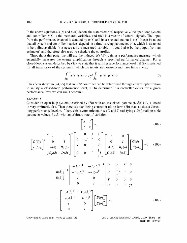
6. LINEAR PARAMETER VARYING CONTROL
With the overall controller structure presented in Section 4, the control objectives given in Section 2,and the choice of performance channels and weights decided in Section 5, the preparations forthe dynamic LPV controller design have been done. This leads to the design of an LPV controllerfor the control of wind turbines. This section will present the base of the algorithm for controllersynthesis and construction.
6.1. Synthesis of LPV controllers
In [20] an analysis is provided for LPV closed-loop systems under the assumption of slowly varyingparameters and in [21, 22] the general framework for designing LPV controllers with arbitrary rateof variation was presented in a linear matrix inequality (LMI) formulation. In the following, thedesign procedure is summarized and it is discussed how to handle numerical difficulties that mightoccur for higher-order systems.
During this section, an abstract representation will be used for the model derived in Section 3combined with the performance weights. We consider a weighted open-loop model of the form(8a), which is created along standard lines for system interconnection as done in [23]. We will thensearch for a controller, (8b), of similar structure as the open-loop model to satisfy a specified closed-loop performance. The model and controller can be interconnected to a closed-loop representationdescribed by short-hand notation in (8c), for which it can be observed that the formulation is affinein the controller variables
⎡⎢⎣x(t)
z(t)
y(t)
⎤⎥⎦ =
⎡⎢⎣
A((t)) Bp((t)) B((t))
Cp((t)) D((t)) E((t))
C((t)) F((t)) 0
⎤⎥⎦
⎡⎢⎣x(t)
w(t)
u(t)
⎤⎥⎦ (8a)
[xc(t)
u(t)
]=
[Ac((t)) Bc((t))
Cc((t)) Dc((t))
][xc(t)
y(t)
](8b)
[xcl(t)
z(t)
]=
[Acl((t)) Bcl((t))
Ccl((t)) Dcl((t))
][xcl(t)
w(t)
](8c)
§The 3P frequency is three times the rotational speed of the rotor.
Copyright q 2008 John Wiley & Sons, Ltd. Int. J. Robust Nonlinear Control 2009; 19:92–116DOI: 10.1002/rnc
102 K. Z. ØSTERGAARD, J. STOUSTRUP AND P. BRATH
In the above equations, x(t) and xc(t) denote the state vector of, respectively, the open-loop systemand controller, y(t) is the measured variables, and u(t) is a vector of control signals. The inputfrom the performance channel is denoted by w(t) and its associated output is z(t). It can be notedthat all system and controller matrices depend on a time-varying parameter, (t), which is assumedto be online available (not necessarily a measured variable—it could also be the output from anestimator) and therefore also used to schedule the controller.
Throughout this paper we will use the induced L2/L2 gain as a performance measure, whichessentially measures the energy amplification through a specified performance channel. For aclosed-loop system described by (8c) we state that it satisfies a performance level if (9) is satisfiedfor all trajectories of the system in which the inputs are non-zero and have finite energy∫ ∞
0z(t)Tz(t)dt<2
∫ ∞
0w(t)Tw(t)dt (9)
It has been shown in [24, 25] that an LPV controller can be determined through convex optimizationto satisfy a closed-loop performance level, . To determine if a controller exists for a givenperformance level we can use Theorem 1.
Theorem 1Consider an open-loop system described by (8a) with an associated parameter, (t)∈�, allowedto vary arbitrarily fast. Then there is a stabilizing controller of the form (8b) that satisfies a closed-loop performance level, , if there exist symmetric matrices X and Y satisfying (10) for all possibleparameter values, ∈�, with an arbitrary rate of variation[
X I
I Y
]�0 (10a)
[C()⊥F()⊥
]T
⎡⎢⎢⎢⎢⎣
I 0
0 I
A() Bp()
Cp() D()
⎤⎥⎥⎥⎥⎦
T⎡⎢⎢⎢⎢⎢⎢⎣
0 0 X 0
0 −I 0 0
X 0 0 0
0 0 01
I
⎤⎥⎥⎥⎥⎥⎥⎦
⎡⎢⎢⎢⎢⎣
I 0
0 I
A() Bp()
Cp() D()
⎤⎥⎥⎥⎥⎦
[C()⊥F()⊥
]≺0 (10b)
[B()T⊥E()T⊥
]T
⎡⎢⎢⎢⎢⎣
−A()T −Cp()T
−Bp()T −D()T
I 0
0 I
⎤⎥⎥⎥⎥⎦
T⎡⎢⎢⎢⎢⎢⎢⎣
0 0 Y 0
0 −1
I 0 0
Y 0 0 0
0 0 0 I
⎤⎥⎥⎥⎥⎥⎥⎦
×
⎡⎢⎢⎢⎢⎣
−A()T −Cp()T
−Bp()T −D()T
I 0
0 I
⎤⎥⎥⎥⎥⎦
[B()T⊥E()T⊥
]�0 (10c)
Copyright q 2008 John Wiley & Sons, Ltd. Int. J. Robust Nonlinear Control 2009; 19:92–116DOI: 10.1002/rnc
LINEAR PARAMETER VARYING CONTROL OF WIND TURBINES 103
The matrix inequalities in Theorem 1 are clearly affine in the variables X and Y . In the contextof controller synthesis, it is typically desirable to determine a controller that minimizes and notonly one that satisfies a pre-specified performance specification. This can be done by bisectionor alternatively by using the well-known Schur lemma, whereby the two matrix inequalities aretransformed into matrix inequalities that are also linear in . Then can be used directly in theoptimization problem.
In the above performance specification, it is required to solve infinitely many LMIs—one foreach possible parameter—and the problem cannot therefore be solved in finite time. In the specialcase of affine parameter dependency and with the parameters varying within a convex polytope,the problem reduces to checking only the vertices [26]. As discussed in the Introduction, affineparameter dependency is not expected to give a satisfactory performance for the application inmind. Alternatively, a method has been developed for designing controllers for the case of rationalparameter dependency [27, 28]. This approach is much more appealing, but suffers from numericalissues in the construction of controllers from the synthesis variables. One issue is that the numericsare highly dependent on the choice (and size) of a linear fractional representation, which makes ita very demanding task to design controllers for which the performance function is scheduled, andthe scheduling might change between iterations in the design process. Because of these reasons,it has been chosen to focus on an approximative method (using a grid) presented in [29] but stillwith the assumption of arbitrarily fast parameter variations.
The density of the grid is to be determined from a trade-off between having a lot of grid pointscausing heavy computational time and a few grid points not catching the nonlinear behaviourto a sufficient degree. It can be shown that if a parameterized LMI is satisfied for two selectedparameter values, the parameterized LMI will also be satisfied for a convex combination of the twoparameters—see, for example [23]. This means that if we can assume affine parameter dependencyof the weighted open loop in the interval between two grid points, the stability and performancewill be given for the intermediate parameter values. For the specific application of LPV controlfor wind turbines, it has been chosen to select two grid points in each of the following threeoperating modes: partial load operation with variable generator speed, partial load operation withnominal generator speed, and full load operation. This provides an acceptable trade-off betweenhaving a few number of grid points and not violating the assumption of piecewise affine parameterdependency too much.
6.2. Controller construction
By solving the optimization problem for controller synthesis in Theorem 1, we get an achievableperformance level, , and the matrices X and Y for the quadratic storage/Lyapunov function usedto measure the performance and stability of the closed-loop interconnection.
Note that the controller variables Ac, Bc, Cc, and Dc are not directly available from Theorem 1.Fortunately, a method for constructing the controller variables has been developed in which an LMIcontaining the controller variables can be constructed and solved analytically from the result of (10).
The details can be found in [24, 25] and in this paper we focus only on the actual procedurefor constructing the controller when X and Y have been determined. To simplify the notation, werewrite (10b) and (10c) as in (11) with the variables defined in (12)
RT⊥
[I
Q
]T
P
[I
Q
]R⊥ ≺ 0 (11a)
Copyright q 2008 John Wiley & Sons, Ltd. Int. J. Robust Nonlinear Control 2009; 19:92–116DOI: 10.1002/rnc
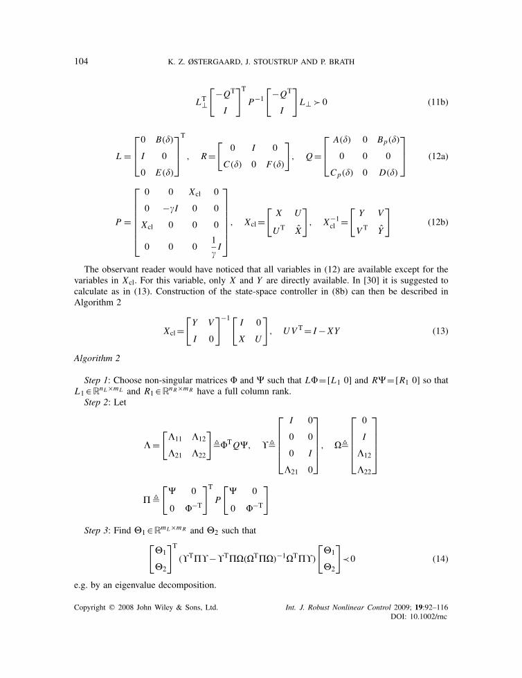
104 K. Z. ØSTERGAARD, J. STOUSTRUP AND P. BRATH
LT⊥
[−QT
I
]T
P−1
[−QT
I
]L⊥ � 0 (11b)
L =⎡⎢⎣0 B()
I 0
0 E()
⎤⎥⎦T
, R=[
0 I 0
C() 0 F()
], Q=
⎡⎢⎣
A() 0 Bp()
0 0 0
Cp() 0 D()
⎤⎥⎦ (12a)
P =
⎡⎢⎢⎢⎢⎢⎢⎣
0 0 Xcl 0
0 −I 0 0
Xcl 0 0 0
0 0 01
I
⎤⎥⎥⎥⎥⎥⎥⎦
, Xcl=[
X U
UT X
], X−1
cl =[Y V
V T Y
](12b)
The observant reader would have noticed that all variables in (12) are available except for thevariables in Xcl. For this variable, only X and Y are directly available. In [30] it is suggested tocalculate as in (13). Construction of the state-space controller in (8b) can then be described inAlgorithm 2
Xcl=[Y V
I 0
]−1[I 0
X U
], UV T= I −XY (13)
Algorithm 2
Step 1: Choose non-singular matrices � and � such that L�=[L1 0] and R�=[R1 0] so thatL1∈RnL×mL and R1∈RnR×mR have a full column rank.
Step 2: Let
� =[
�11 �12
�21 �22
]��TQ�, ��
⎡⎢⎢⎢⎢⎣
I 0
0 0
0 I
�21 0
⎤⎥⎥⎥⎥⎦ , ��
⎡⎢⎢⎢⎢⎣
0
I
�12
�22
⎤⎥⎥⎥⎥⎦
� �[
� 0
0 �−T
]T
P
[� 0
0 �−T
]
Step 3: Find �1∈RmL×mR and �2 such that[�1
�2
]T
(�T��−�T��(�T��)−1�T��)
[�1
�2
]≺0 (14)
e.g. by an eigenvalue decomposition.
Copyright q 2008 John Wiley & Sons, Ltd. Int. J. Robust Nonlinear Control 2009; 19:92–116DOI: 10.1002/rnc
LINEAR PARAMETER VARYING CONTROL OF WIND TURBINES 105
Step 4: Then [Ac() Bc()
Cc() Dc()
]= L−T
1 (�2�−11 −�11)R
−11
7. NUMERICAL CONDITIONING OF AN LPV CONTROLLER DESIGN
To summarize we have seen that the LPV controller design problem can be solved by determiningX and Y satisfying (10) for which is minimized. Then Xcl can be constructed using (13), andthe controller matrices in K can then be determined by Algorithm 2 with variables as in (12).In practice, the solution is unfortunately not that simple because numerical issues might makethe controller construction impossible if no extra measures are taken. This section will presentmethods for conditioning the controller synthesis and construction to make it possible to designLPV controllers for practical applications.
7.1. Inversion of �T��
It can be shown that (11a) is equivalent to requiring �T��≺0. This means that �T�� is alwaysnon-singular, but in practice it might become very ill-conditioned which can be seen from theparticular set-up for control of wind turbines. In this application, the primal LMI has a conditionnumber in the order of 1010 and it is concluded that the inversion of a matrix that is ill-conditionedmight affect the numerical conditioning of the algorithm. In [31] a remedy is suggested by anappropriate scaling of �.
Choose � such that R�=[R1 0] as in Algorithm 2, e.g. by a singular value decompositionof R. Then let
J =[J11 J12
J21 J22
]=�
T[I
Q
]T
P
[I
Q
]�, �=�
[I 0
0 Q
], QTQ=−J−1
22
We can observe that � satisfies the condition R�=[R1 0], now with �T��≈−I . We are ofcourse still left with finding a suitable Q, which is not easier from a numerical point of view, butthe point is that even with an approximate solution �T�� is made better conditioned.
7.2. Conditioning of variables
The main matrix inequality used to determine the controller variables is (14), which containsa number of products between matrices, �, �, and �. If one or more of these variables areill-conditioned, numerical errors might make small negative eigenvalues of (14) shift to positiveeigenvalues, which in the end means that it is impossible to determine �1 and �2 of appropriatedimension that renders the matrix inequality satisfied.
The conditioning of � and � is given mainly by the norm of Q and �, because they are boundedfrom below by 1. If a proper realization is chosen (e.g. according to the discussion above andby scaling of the inputs and outputs), the norm of Q will not have any significant impact on thenumerical stability of the algorithm. The norm of � will be given mainly by the square root of J22,which is expected to have a norm in the same scale as P . This means that with a proper choice of
Copyright q 2008 John Wiley & Sons, Ltd. Int. J. Robust Nonlinear Control 2009; 19:92–116DOI: 10.1002/rnc
106 K. Z. ØSTERGAARD, J. STOUSTRUP AND P. BRATH
realization and scaling of inputs and outputs, the numerical issues in controller construction withthe proposed algorithm is determined by the conditioning of � and thereby P .
For reasonable choices of performance level ( close to 1), the conditioning of P is given bythe conditioning of Xcl. Xcl is unfortunately often close to being singular when the optimiza-tion problem approaches optimum. A remedy is to take advantage of the partitioning used forconstructing Xcl. In [23], four different modifications to (11) have been investigated and it hasbeen found promising to modify the variables for the construction algorithm in order to distributethe conditioning more evenly. This can be done by performing the variable substitution in (15)
Pnew=
⎡⎢⎢⎢⎢⎢⎢⎢⎣
0 0 X−11 0
0 −I 0 0
X−T1 0 0 0
0 0 01
I
⎤⎥⎥⎥⎥⎥⎥⎥⎦
, Qnew=[X2 0
0 I
]Q, Lnew= L
[XT2 0
0 I
](15)
We now need to choose X1 and X2 appropriately in order to optimize numerical performance.Three different approaches have been investigated in [23] and it has been found that methodpresented in the following has superior performance.
We will take advantage of the requirement of X and Y being symmetric and positive definite.This means that they can be expressed as X =MTM and Y =NTN , e.g. by a Cholesky factorization.Then (13) can be rearranged as (16)
Xcl=[NTN V
I 0
]−1[I 0
MTM U
]=
[N N−TV
M−T 0
]−1[N−T 0
M M−TU
](16)
If we denote
ST T=M−TUV TN−1=M−TN−1−MNT (17)
we can describe X1 and X2 in the following equation:
X1=[
N T
M−T 0
], X2=
[N−T 0
M S
](18)
7.3. Bounding synthesis LMIs and variables
The remedies presented in Sections 7.1 and 7.2 involve modifications to the construction algo-rithm to render the controller construction possible from a numerical point of view. In practicalapplications, the controller construction might still fail because of numerical issues.
For a typical application, X and Y will become large when reaching optimum and I −XY willbe close to singular. This means that the construction of X1 and X2 of full rank is difficult becauseU or V (or equivalently S and T ) will be ill-conditioned. In the particular application, this isalso the case with I −XY having a condition number in the order of 1013. To handle this issuea slack variable � has been included in the coupling condition (10a) as in (19) to separate the
Copyright q 2008 John Wiley & Sons, Ltd. Int. J. Robust Nonlinear Control 2009; 19:92–116DOI: 10.1002/rnc
LINEAR PARAMETER VARYING CONTROL OF WIND TURBINES 107
eigenvalues of X from the eigenvalues of Y−1. With a Schur complement of (19) and a reorderingof the terms, we can see that I −XY ≺−(�2−1)I which means that by increasing � we can makeI −XY better conditioned [
Y �I
�I X
]�0 (19)
As mentioned, X and Y might also become very large in norm which increases the norm ofX1 and X2 and in many cases making them worse-conditioned. To avoid this an upper bound isincluded for the two variables.
It should be noted that these introduced coefficients and bounds come with the cost that thesynthesis problem in Theorem 1 most likely will not satisfy the performance criterion, , with theintroduced bounds. This means that it might be necessary to go for a controller satisfying a slightlypoorer performance level. For the particular application, this means a decrease in performancefrom =1 to =1.33.
7.4. Design algorithm
In summary we can design a controller to satisfy a given performance specification by followingAlgorithm 3.
Algorithm 3
Step 1: Determine X and Y by solving the set of LMIs in Theorem 1.Step 2: Determine a representation for X1 and X2 according to (18).Step 3: Calculate the controller, K , from Algorithm 2 with the suggested modifications.Step 4: If controller construction fails, bound critical variables/LMIs and reiterate from Step 2.
8. SIMULATION RESULTS
The proposed design algorithm has been applied to the control of wind turbines. The gain and timeconstant in the performance weights have been chosen by an iterative procedure by first designinga linear time invariant (LTI) controller at the operating points to satisfy the desired performancespecifications after which the LPV controller is designed. This design has resulted in the controllerillustrated in Figure 6 in which the most noticeable observation is the switch between mainly usinga generator torque at low wind speeds and a pitch at high wind speeds.
In the design procedure it was experienced that it was necessary to exaggerate the gain of theperformance weights to get appropriate performance from a simulations point of view. Especiallythe weight on pitch at low wind speeds, tracking error of generator speed at mid wind speeds, andgenerator torque at high wind speeds needed to be modified significantly from the LTI design tothe LPV design to get similar controllers. Otherwise, the LPV controller in low wind speed wouldresemble the high wind speed controller too much. It will be shown that the LPV controller designedusing the exaggerated performance weights show satisfactory performance from simulations pointof view, and the LPV controller design is therefore concluded to be successful.
Copyright q 2008 John Wiley & Sons, Ltd. Int. J. Robust Nonlinear Control 2009; 19:92–116DOI: 10.1002/rnc
108 K. Z. ØSTERGAARD, J. STOUSTRUP AND P. BRATH
–80
–60
– 40
– 20
0
20
Qg,
ref
ωerr pt,acc
100 101 102 103
–80
– 60
– 40
–20
0
β ref
Freq. [rad/s]100 101 102 103
Freq. [rad/s]
vv
vv
Figure 6. Magnitude plot of LPV controller. Dark shades represent low wind speeds andlight shades represent high wind speeds.
full/partial load
PID
PID
Windturbine
generatorReference
ref
β
P
v
gω
refP
refβ
v
hub
opt
rated
ω +
+
Figure 7. Block diagram of a classical controller.
8.1. Simulation set-up
A controller similar to a commercial controller has been used for simulation-based illustrations ofthe benefits of the designed LPV controller. In Figure 7 a rough sketch of this classical controlleris presented and in what follows it will be described briefly.
The main part of the controller is a set of two proportional integral derivatives (PIDs) for trackingof generator speed. In partial load operation, one PID controller is used which has power referenceas a control signal. Another PID controller is used in full load operation with pitch reference ascontrol signal. These PID controllers are gain scheduled on the basis of generator speed and pitch
Copyright q 2008 John Wiley & Sons, Ltd. Int. J. Robust Nonlinear Control 2009; 19:92–116DOI: 10.1002/rnc
LINEAR PARAMETER VARYING CONTROL OF WIND TURBINES 109
angle in order to take into account the variations in the aerodynamics. They have been tuned bythe Ziegler–Nichols approach and are implemented with anti-windup to take into account thatthe control signals can be saturated. In Figure 7, a simple switching mechanism is illustrated todecide if the partial load controller or the full load controller is active. This is a simplificationof the real implementation, because means have been included to allow for bumpless transferbetween the two controllers. To minimize drive train oscillations, an additional loop is includedwhich updates the power reference on the basis of generator speed variations around the drive traineigenfrequency.
The closed-loop performance has then been evaluated through simulations of both the classicalcontroller and the LPV controller. These simulations have been performed with a stochastic windinput with turbulence according to the IEC 1A standard [32].
The performance criteria for the tracking of generator speed and active power will be measureddifferently in partial load and full load operations. In partial load operation, the tracking will bemeasured by average power production during the entire simulation. In full load operation, thetracking of power production is measured by the standard deviation on active power. For thisperformance criterion, time ranges are disregarded where either controller is operating in partialload. Further, in operation modes with rated generator speed, the tracking of the generator speedis measured by the difference between minimum and maximum generator speeds.
The performance for especially the fatigue damage is difficult to evaluate directly from theenergy gain as discussed in [13], and the damage on tower and drive train is evaluated fromrain-flow count [33]. Finally, the damage due to pitch activity is mostly on the blade bearings forwhich the damage can be approximated by the standard deviation of the pitch rate [33].
8.2. Partial load and variable-speed operations
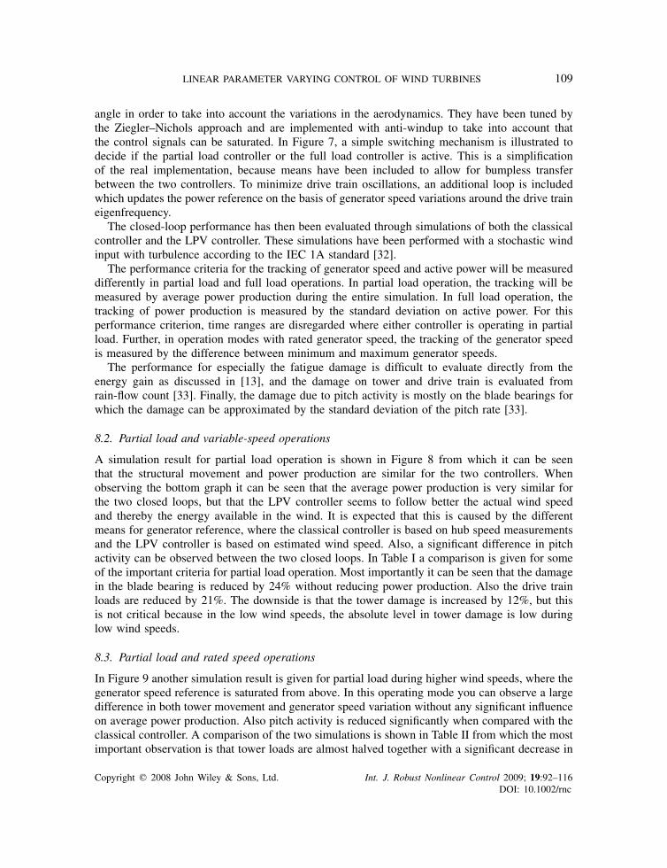
A simulation result for partial load operation is shown in Figure 8 from which it can be seenthat the structural movement and power production are similar for the two controllers. Whenobserving the bottom graph it can be seen that the average power production is very similar forthe two closed loops, but that the LPV controller seems to follow better the actual wind speedand thereby the energy available in the wind. It is expected that this is caused by the differentmeans for generator reference, where the classical controller is based on hub speed measurementsand the LPV controller is based on estimated wind speed. Also, a significant difference in pitchactivity can be observed between the two closed loops. In Table I a comparison is given for someof the important criteria for partial load operation. Most importantly it can be seen that the damagein the blade bearing is reduced by 24% without reducing power production. Also the drive trainloads are reduced by 21%. The downside is that the tower damage is increased by 12%, but thisis not critical because in the low wind speeds, the absolute level in tower damage is low duringlow wind speeds.
8.3. Partial load and rated speed operations
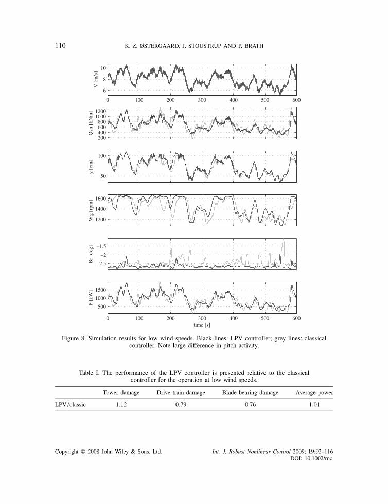
In Figure 9 another simulation result is given for partial load during higher wind speeds, where thegenerator speed reference is saturated from above. In this operating mode you can observe a largedifference in both tower movement and generator speed variation without any significant influenceon average power production. Also pitch activity is reduced significantly when compared with theclassical controller. A comparison of the two simulations is shown in Table II from which the mostimportant observation is that tower loads are almost halved together with a significant decrease in
Copyright q 2008 John Wiley & Sons, Ltd. Int. J. Robust Nonlinear Control 2009; 19:92–116DOI: 10.1002/rnc
110 K. Z. ØSTERGAARD, J. STOUSTRUP AND P. BRATH
0 100 200 300 400 500 600
6
8
10
V [
m/s
]
200400600800
10001200
Qsh
[kN
m]
50
100
y [c
m]
1200
1400
1600
Wg
[rpm
]B
r [d
eg]
0 100 200 300 400 500 600
500
1000
1500
–1.5
–2
–2.5
P [k
W]
time [s]
Figure 8. Simulation results for low wind speeds. Black lines: LPV controller; grey lines: classicalcontroller. Note large difference in pitch activity.
Table I. The performance of the LPV controller is presented relative to the classicalcontroller for the operation at low wind speeds.
Tower damage Drive train damage Blade bearing damage Average power
LPV/classic 1.12 0.79 0.76 1.01
Copyright q 2008 John Wiley & Sons, Ltd. Int. J. Robust Nonlinear Control 2009; 19:92–116DOI: 10.1002/rnc
LINEAR PARAMETER VARYING CONTROL OF WIND TURBINES 111
0 100 200 300 400 500 600
10
15
V [
m/s
]
1000
1500
2000
Qsh
[kN
m]
50
100
150
y [c
m]
1550160016501700
Wg
[rpm
]
02468
Br
[deg
]
0 100 200 300 400 500 6001000
2000
3000
P [k
W]
time [s]
Figure 9. Simulation results for medium wind speeds. Black lines: LPV controller; grey lines: classicalcontroller. Note large difference in tower movement and generator speed.
Table II. The performance of the LPV controller is presented relative to the classicalcontroller for the operation at medium wind speeds.
Tower damage Drive train damage Blade bearing damage Speed peak–peak Average power
LPV/classic 0.48 0.93 0.70 0.68 1.00
Copyright q 2008 John Wiley & Sons, Ltd. Int. J. Robust Nonlinear Control 2009; 19:92–116DOI: 10.1002/rnc
112 K. Z. ØSTERGAARD, J. STOUSTRUP AND P. BRATH
0 100 200 300 400 500 600
1214161820
V [
m/s
]
120014001600180020002200
Qsh
[kN
m]
406080
100120140
y [c
m]
1500
1600
1700
Wg
[rpm
]
0
5
10
15
Br
[deg
]
0 100 200 300 400 500 600
2000
2500
3000
P [k
W]
time [s]
Figure 10. Simulation results for high wind speeds. Black lines: LPVcontroller; grey lines: classical controller.
generator speed of 32%. This is obtained without increasing the pitch activity or decreasing theaverage power production.
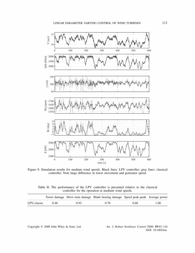
8.4. Full load operation
In full load operation, improvements can be observed when compared with the classical controller.A result from a simulation in full load is given in Figure 10 in which the most important observationis that the generator speed variations are reduced significantly without increasing structural loads.A number of power dips are also observed in the classical controller due to switching to partialload operation. The difference between the two controllers is caused by the different means for
Copyright q 2008 John Wiley & Sons, Ltd. Int. J. Robust Nonlinear Control 2009; 19:92–116DOI: 10.1002/rnc
LINEAR PARAMETER VARYING CONTROL OF WIND TURBINES 113
Table III. The performance of the LPV controller is presented relative to the classicalcontroller for the operation at high wind speeds.
Tower damage Drive train damage Blade bearing damage Speed peak–peak Std. power
LPV/classic 0.85 0.56 0.98 0.67 0.94
generator references as discussed in Section 8.2. From a comparison given in Table III, it can beobserved that the generator speed is reduced by 33% and drive train oscillations are reduced by44% without increasing pitch activity, power fluctuations, or tower oscillations.
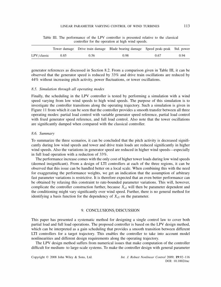
8.5. Simulation through all operating modes
Finally, the scheduling in the LPV controller is tested by performing a simulation with a windspeed varying from low wind speeds to high wind speeds. The purpose of this simulation is toinvestigate the controller transitions along the operating trajectory. Such a simulation is given inFigure 11 from which it can be seen that the controller provides a smooth transfer between all threeoperating modes: partial load control with variable generator speed reference, partial load controlwith fixed generator speed reference, and full load control. Also note that the tower oscillationsare significantly damped when compared with the classical controller.
8.6. Summary
To summarize the three scenarios, it can be concluded that the pitch activity is decreased signifi-cantly during low wind speeds and tower and drive train loads are reduced significantly in higherwind speeds. Also the variations in generator speed are reduced in higher wind speeds—especiallyin full load operation with a reduction of 33%.
The performance increase comes with the only cost of higher tower loads during low wind speeds(deemed insignificant). From a design of LTI controllers at each of the three regions, it can beobserved that this issue can be handled better on a local scale. When combining this with the needfor exaggerating the performance weights, we get an indication that the assumption of arbitraryfast parameter variations is restrictive. It is therefore expected that an even better performance canbe obtained by relaxing this constraint to rate-bounded parameter variations. This will, however,complicate the controller construction further, because Xcl will then be parameter dependent andthe conditioning might vary significantly over wind speed. Further, there is no general method foridentifying a basis function for the dependency of Xcl on the parameter.
9. CONCLUSIONS/DISCUSSION
This paper has presented a systematic method for designing a single control law to cover bothpartial load and full load operations. The proposed controller is based on the LPV design method,which can be interpreted as a gain scheduling that provides a smooth transition between differentLTI controllers for a target trajectory. This enables the controller to take into account modelnonlinearities and different design requirements along the operating trajectory.
The LPV design method suffers from numerical issues that make computation of the controllerdifficult for medium- to large-scale systems. To make the controller design with general parameter
Copyright q 2008 John Wiley & Sons, Ltd. Int. J. Robust Nonlinear Control 2009; 19:92–116DOI: 10.1002/rnc
114 K. Z. ØSTERGAARD, J. STOUSTRUP AND P. BRATH
0 100 200 300 400 500 60068
1012141618
V [
m/s
]
1000
2000
Qsh
[kN
m]
50
100
y [c
m]
1400
1600
Wg
[rpm
]
0
5
10
Br
[deg
]
0 100 200 300 400 500 600
1000
2000
3000
P [k
W]
time [s]
Figure 11. Simulation results for whole wind speed range. Black lines: LPV controller; grey lines: classicalcontroller. Note smooth transition between operating modes and reduced tower oscillations.
dependency possible for the specific application, the paper has presented and discussed severalissues related to the numerical computation of LPV controllers.
The proposed method for obtaining a numerically stable design algorithm has been used forthe design of an LPV controller for control of wind turbines in both partial load and full loadoperations. Using simulation studies, the proposed controller has been compared with a controllerdesigned using classical techniques and it has been concluded that the LPV controller achievessignificantly better performance. Most importantly, a decrease in pitch activity is observed for lowwind speeds and tower and drive train loads are reduced in higher wind speeds. This performanceincrease is obtained without affecting the produced power, power fluctuations, and generator speed
Copyright q 2008 John Wiley & Sons, Ltd. Int. J. Robust Nonlinear Control 2009; 19:92–116DOI: 10.1002/rnc
LINEAR PARAMETER VARYING CONTROL OF WIND TURBINES 115
variations. However, the tower loads are observed to increase slightly during low wind speeds, butthis increase is deemed insignificant and the design is therefore concluded to be successful.
The proposed controller has not yet been implemented on a real wind turbine. Before this can bedone it should be investigated how the control law affects the structural components not includedin the design model, e.g. blade dynamics and tower sideways movement.
Finally, it has been experienced that there is a large difference between the combination ofweights that are appropriate for designing local H∞ controllers and the weights necessary forappropriate simulation results in the LPV framework. For the weights for the LPV control, it wasnecessary to exaggerate the weights to get the desired performance from a simulation point ofview. This indicates that the assumption of arbitrarily fast parameter variations is conservative andit is therefore suggested to do similar investigations for rate-bounded parameter variations. Thedesign algorithm in this case is in theory very similar, but the numerics are expected to be moredifficult to handle, because conditioning of the design variables can vary more over the operatingtrajectory.
As a concluding remark it should be noted that model uncertainty is not handled directly in thedesign formulation, but the performance channels considering tower and drive train oscillationscan be considered as a detuning of the tracking controller at the two respective eigenfrequencies.Also the channels from disturbance (wind speed) to control signals can be considered similar tothe control sensitivity usually used in robust controller techniques. Robustness towards parametricuncertainty can be covered fairly well by sampling the parameter space.
ACKNOWLEDGEMENTS
The authors would like to thank Professor C. Scherer from Delft University of Technology, The Netherlands,for his helpful discussions about the numerics related to controller construction for LPV controllers.
REFERENCES
1. Gardner P, Garrad A, Jamieson P, Snodin H, Nichols G, Tindal A. Wind energy—the facts—volume 1. TechnicalReport, Garrad Hassan for European Wind Energy Association, 2002.
2. Hand MM, Balas MJ. Systematic controller design methodology for variable-speed wind turbines. TechnicalReport, NREL, 2002.
3. Vihriala H, Ridanpaa P, Perala R, Soderlund L. Control of a variable speed wind turbine with feedforward ofaerodynamic torque. European Wind Energy Conference, Nice, France, 1999; 881–884.
4. Connor B, Leithead WE, Grimble MJ. LQG control of a constant speed horizontal axis wind turbine. Conferenceon Control Applications, Glasgow, Scotland, 1994; 251–252. DOI: 10.1109/CCA.1994.381190.
5. Munteanu I, Cutululis NA, Bratcu AI, Ceanga E. Optimization of variable speed wind power systems based ona LQG approach. Control Engineering Practice 2004; 13(7):903–912. DOI: 10.1016/j.conengprac.2004.10.013.
6. Rocha R, Filho LSM, Bortolus MV. Optimal multivariable control for wind energy conversion system—acomparison between H2 and H∞ controllers. Conference on Decision and Control, Seville, Spain, 2005;7906–7911.
7. Cutululis NA, Ceanga E, Hansen AD, Sørensen P. Robust multi-model control of an autonomous wind powersystem. Wind Energy 2006; 9:399–419. DOI: 10.1002/we.194.
8. Jelavic M, Peric N, Petrovic I, Car S, Madercic M. Design of a wind turbine pitch controller for loads andfatigue reduction. European Wind Energy Conference, Milan, Italy, 2007.
9. Kraan I, Bongers PMM. Control of a wind turbine using several linear robust controllers. Conference on Decisionand Control, San Antonio, TX, U.S.A., 1993; 1928–1929. DOI: 10.1109/CDC.1993.325530.
10. Leith DJ, Leithead WE. Application of nonlinear control to a HAWT. Conference on Control Applications,Glasgow, Scotland, 1994; 245–250. DOI: 10.1109/CCA.1994.381191.
Copyright q 2008 John Wiley & Sons, Ltd. Int. J. Robust Nonlinear Control 2009; 19:92–116DOI: 10.1002/rnc
116 K. Z. ØSTERGAARD, J. STOUSTRUP AND P. BRATH
11. Leith DJ, Leithead WE. Appropriate realization of gain-scheduled controllers with application to wind turbineregulation. International Journal of Control 1996; 65(2):223–248. DOI: 10.1080/00207179608921695.
12. van Engelen TG, van der Hooft EL, Schaak P. Development of wind turbine control algorithms for industrialuse. European Wind Energy Conference, Madrid, Spain, 2003.
13. Lescher F, Camblong H, Curea O, Briand R. LPV control of wind turbines for fatigue loads reduction usingintelligent micro sensors. American Control Conference, New York City, NY, U.S.A., 2007; 6061–6066.
14. Lescher F, Zhao JY, Borne P. Robust gain scheduling controller for pitch regulated variable speed wind turbine.Studies in Informatics and Control 2005; 14(4):299–315.
15. Mantz RJ, Bianchi FD, Christiansen CF. Gain scheduling control of variable-speed wind energy conversion systemsusing quasi-LPV models. Control Engineering Practice 2005; 13:247–255. DOI: 10.1016/j.conengprac.2004.03.006.
16. Balas GJ. Linear, parameter-varying control and its applications to a turbofan engine. International Journal ofRobust and Nonlinear Control 2002; 12:763–796. DOI: 10.1002/rnc.704.
17. Burton T, Sharpe D, Jenkins N, Bossanyi EA. Wind Energy Handbook. Wiley: New York, 2001. DOI: 10.1002/0470846062.
18. Østeraard KZ, Brath P, Stoustrup J. Estimation of effective wind speed. Journal of Physics: Conference Series2007; 75. Available at: http://www.iop.org/EJ/toc/1742-6596/75/1.
19. Howze JW, Bhattacharyya SP. Robust tracking, error feedback, and two-degree-of-freedom controllers.Transactions on Automatic Control 1997; 42(7):980–983.
20. Shamma JS, Athans M. Analysis of gain scheduled control for nonlinear plants. Transactions on AutomaticControl 1990; 35(8):898–907. DOI: 10.1109/9.58498.
21. Becker G, Packard A. Robust performance of linear parametrically varying systems using parametrically-dependentlinear feedback. Systems and Control Letters 1994; 23:205–215. DOI: 10.1016/0167-6911(94)90006-X.
22. Gahinet P, Apkarian P. A linear matrix inequality approach to H∞ control. International Journal of Robust andNonlinear Control 1994; 4:421–448. DOI: 10.1002/rnc.4590040403.
23. Østergaard KZ. Robust, gain-scheduled control of wind turbines. Ph.D. Thesis, Aalborg University, 2008.24. Helmersson A. IQC synthesis based on inertia constraints. IFAC World Congress, Beijing, China, 1999.25. Scherer CW. Recent Advantages on LMI Methods in Control. Chapter: Robust mixed control and LPV control
with full block scalings. SIAM: Philadelphia, PA, 2000.26. Apkarian P, Gahinet P, Becker G. Self-scheduled H∞ control of linear parameter-varying systems—a design
example. Automatica 1995; 31(9):1251–1261. DOI: 10.1016/0005-1098(95)00038-X.27. Scherer CW. LPV control and full block multipliers. Automatica 2001; 37:361–375.28. Iwasaki T, Shibata G. LPV system analysis via quadratic separator for uncertain implicit systems. Transactions
on Automatic Control 2001; 46(8):1195–1208. DOI: 10.1109/9.940924.29. Wu F, Yang XH, Packard A, Becker G. Induced L2-norm control for LPV system with bounded parameter
variation rates. American Control Conference, Seattle, Washington, U.S.A., 1995; 2379–2383.30. Gahinet P. Explicit controller formulas for LMI-based H∞ synthesis. Automatica 1996; 32(7):1007–1014. DOI:
10.1016/0005-1098(96)00033-7.31. Trangbæk K. Linear parameter varying control of induction motors. Ph.D. Thesis, Aalborg University, 2001.32. IEC. IEC 61400-1. International Standard, 2005.33. Hammerum K. A fatigue approach to wind turbine control. Master’s Thesis, Technical University of Denmark,
2006.
Copyright q 2008 John Wiley & Sons, Ltd. Int. J. Robust Nonlinear Control 2009; 19:92–116DOI: 10.1002/rnc