HAL Id: hal-00727039https://hal.archives-ouvertes.fr/hal-00727039v3

Preprint submitted on 29 Apr 2013

HAL is a multi-disciplinary open accessarchive for the deposit and dissemination of sci-entific research documents, whether they are pub-lished or not. The documents may come fromteaching and research institutions in France orabroad, or from public or private research centers.

L’archive ouverte pluridisciplinaire HAL, estdestinée au dépôt et à la diffusion de documentsscientifiques de niveau recherche, publiés ou non,émanant des établissements d’enseignement et derecherche français ou étrangers, des laboratoirespublics ou privés.

Linear programming formulations for queueing controlproblems with action decomposabilityAriel Waserhole, Jean-Philippe Gayon, Vincent Jost

To cite this version:Ariel Waserhole, Jean-Philippe Gayon, Vincent Jost. Linear programming formulations for queueingcontrol problems with action decomposability. 2012. �hal-00727039v3�

Linear programming formulations for queueing control

problems with action decomposability

Ariel Waserhole 1,2 Jean-Philippe Gayon1 Vincent Jost2

1 G-SCOP, Grenoble-INP 2 LIX CNRS, Ecole Polytechnique Palaiseau

April 26, 2013

Abstract

We consider a special class of continuous-time Markov decision processes (CTMDP) that areaction decomposable. An action-Decomposed CTMDP (D-CTMPD) typically models queueingcontrol problems with several types of events. A sub-action and cost is associated to each typeof event. The action space is then the Cartesian product of sub-action spaces. We first proposea new and natural Quadratic Programming (QP) formulation for CTMDPs and relate it to moreclassic Dynamic Programming (DP) and Linear Programming (LP) formulations. Then we focuson D-CTMDPs and introduce the class of decomposed randomized policies that will be shownto be dominant in the class of deterministic policies by a polyhedral argument. With this newclass of policies, we are able formulate decomposed QP and LP with a number of variables linearin the number of types of events whereas in its classic version the number of variables growsexponentially. We then show how the decomposed LP formulation can solve a wider class ofCTMDP that are quasi decomposable. Indeed it is possible to forbid any combination of sub-actions by adding (possibly many) constraints in the decomposed LP. We prove that, given a set oflinear constraints added to the LP, determining whether there exists a deterministic policy solutionis NP-complete. We also exhibit simple constraints that allow to forbid some specific combinationsof sub-actions. Finally, a numerical study compares computation times of decomposed and non-decomposed formulations for both LP and DP algorithms.

Keywords: Continuous-time Markov decision process; Queueing control; Event-based dynamicprogramming; Linear programming.

1 Introduction

Different approaches exist to solve numerically a Continuous-Time Markov Decision Problem (CT-MDP) that are based on optimality equations (or Bellman equations). The most popular methodis the value iteration algorithm which is essentially a backward Dynamic Programming (DP). An-other well known approach is to model a CTMDP as a Linear Programming (LP). LP based algo-rithms are slower than DP based algorithms. However, LP formulations offer the possibility to addvery easily linear constraints on steady state probabilities, which is not the case of DP formulations.

1

Good introductions to CTMDPs can be found in the books of Puterman (1994), Bertsekas (2005) andGuo and Hernandez-Lerma (2009).

In this paper, we consider a special class of CTMDPs that we call action Decomposed CTMDPs(D-CTMPDs). D-CTMDP typically model queueing control problems with several types of events(demand arrival, service end, failure, etc) and where a sub-action (admission, routing, repairing, etc)and also a cost is associated to each type of event. The class of D-CTMPD is related to the conceptof event-based DP, first introduced by Koole (1998). Event-based DP is a systematic approach forderiving monotonicity results of optimal policies for various queueing and resource sharing models.Citing Koole: “Event-based DP deals with event operators, which can be seen as building blocks ofthe value function. Typically it associates an operator with each basic event in the system, such asan arrival at a queue, a service completion, etc. Event-based DP focuses on the underlying propertiesof the value and cost functions, and allows us to study many models at the same time.” The event-based DP framework is strongly related to older works (see e.g. Lippman (1975); Weber and Stidham(1987)).

Apart from the ability to prove structural properties of the optimal policy, the event-based DPframework is also a very natural way to model many queueing control problems. In addition, it allowsto reduce drastically the number of actions to be evaluated in the value iteration algorithm. Thefollowing example will be used throughout the paper to illustrate our approach and results and will bereferred to as the dynamic pricing problem.

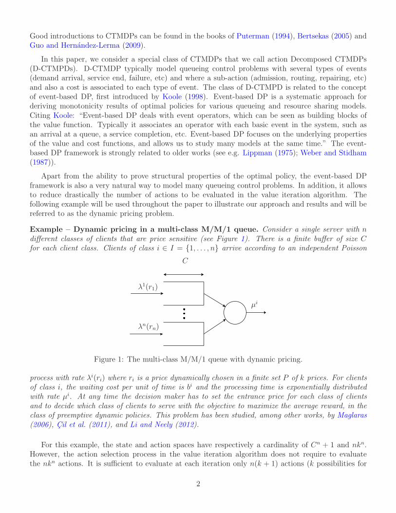
Example – Dynamic pricing in a multi-class M/M/1 queue. Consider a single server with ndifferent classes of clients that are price sensitive (see Figure 1). There is a finite buffer of size Cfor each client class. Clients of class i ∈ I = {1, . . . , n} arrive according to an independent Poisson

λ1(r1)

λn(rn)

µi

C

Figure 1: The multi-class M/M/1 queue with dynamic pricing.

process with rate λi(ri) where ri is a price dynamically chosen in a finite set P of k prices. For clientsof class i, the waiting cost per unit of time is bi and the processing time is exponentially distributedwith rate µi. At any time the decision maker has to set the entrance price for each class of clientsand to decide which class of clients to serve with the objective to maximize the average reward, in theclass of preemptive dynamic policies. This problem has been studied, among other works, by Maglaras(2006), Cil et al. (2011), and Li and Neely (2012).

For this example, the state and action spaces have respectively a cardinality of Cn + 1 and nkn.However, the action selection process in the value iteration algorithm does not require to evaluatethe nkn actions. It is sufficient to evaluate at each iteration only n(k + 1) actions (k possibilities for

2

each class of customer and n possibilities for the class to be served). This property has been usedintensively in the literature since the seminal paper of Lippman (1975). In the classic LP formulationof the dynamic pricing problem, that one can find in (Puterman, 1994) for instance, the number ofvariables grows exponentially with the number of possible prices. In this paper, we will show that theLP can be reformulated in a way such that the number of variables grows linearly with the number ofpossible prices.

Our contributions can be summarized as follows. We first propose a new and natural QuadraticProgramming (QP) formulation for CTMDP and relate it to more classic Dynamic Programming(DP) and Linear Programming (LP) formulations. Then, we introduce the class of D-CTMPDs whichis probably the largest class of CTMDPs for which the event-based DP approach can be used. Wealso introduce the class of decomposed randomized policies that will be shown to be dominant amongrandomized policies. With these new policies, we are able to reformulate the QP and the LP with anumber of variables growing linearly with the number of event types. With respect to the decomposedDP, this LP formulation is really simple to write and does not need the uniformization process necessaryfor the DP formulation which is sometimes source of errors and waste of time. Moreover, it allows touse generic LP related techniques such that sensitivity analysis (Filippi, 2011) or approximate linearprogramming (Dos Santos Eleutrio, 2009).

Another contribution of the paper is to show how to forbid some actions while preserving thestructure of the decomposed LP. If some actions (combinations of sub-actions) are forbidden, the DPcannot be decomposed anymore. In the dynamic pricing example, imagine that we want a low price tobe selected for at least one class of customer. In the (non-decomposed) DP formulation, it is easy toadd this constraint by removing all actions that does not contain a low price. However, it is not possibleto decompose anymore the DP, in our opinion. In the decomposed LP formulation, we show how it ispossible to remove this action and other combinations of actions by adding simple linear constraints.We also discuss the generic problem of reducing arbitrarily the action space by adding a set of linearconstraints in the decomposed LP. Not surprisingly, this problem is difficult and is not appropriate ifmany actions are removed arbitrarily. When new constraints are added in the decomposed LP, it is alsonot clear whether deterministic policies remain dominant or not. We even prove that, given a set oflinear constraints added to the LP, determining whether there exists a deterministic policy solution isNP-complete. However, for some simple action reductions, we show that deterministic policies remaindominant. We finally present numerical results comparing LP and DP formulations (decomposed ornot).

Before presenting the organization of the paper, we mention briefly some related literature address-ing MDP with large state space (Bertsekas and Castanon, 1989; Tsitsiklis and Van Roy, 1996) whichtries to fight the curse of dimensionality, i.e. the exponential growth of the state space size with someparameter of the problem. Another issue, less tackled, appears when the state space is relatively smallbut the action space is very large. Hu et al. (2007) proposes a randomized search method for solvinginfinite horizon discounted cost discrete-time MDP for uncountable action spaces.

The rest of the paper is organized as follows. We first address the average cost problem. Section 2reminds the definition of a CTMDP and formulates it as a QP. We also link the QP formulation withclassic LP and DP formulations. In Section 3, we define properly D-CTMDP and show how the DPand LP can be decomposed for this class of problems. Section 4 discusses the problem of reducingthe action space by adding valid constraints in the decomposed LP. Section 5 compares numericallycomputation times of decomposed and non-decomposed formulations for both LP and DP algorithms,

3

for the dynamic pricing problem. Finally, Section 6 explains how our results can be adapted to adiscounted cost criterion.

2 Continuous-Time Markov Decision Processes

In this section, we remind some classic results on CTMDPs that will be useful to present our contri-butions.

2.1 Definition

We slightly adapt the definition of a CTMDP given by Guo and Hernandez-Lerma (2009). A CTMDPis a stochastic control problem defined by a 5-tuple

{S, A, λs,t(a), hs(a), rs,t(a)

}

with the following components:

• S is a finite set of states;

• A is a finite set of actions, A(s) are the actions available from state s ∈ S;

• λs,t(a) is the transition rate to go from state s to state t with action a ∈ A(s);

• hs(a) is the reward rate while staying in state s with action a ∈ A(s);

• rs,t(a) is the instant reward to go from state s to state t with action a ∈ A(s).

Instant rewards rs,t(a) can be included in the reward rates hs(a) by an easy transformation andreciprocally. Therefore for ease of presentation, we will use the aggregated reward rate hs(a) :=hs(a) +

∑t∈S λs,t(a)rs,t(a).

We first consider the objective of maximizing the average reward over an infinite horizon, thediscounted case will be discussed in the Section 6. We restrict our attention to stationary policieswhich are dominant for this problem (Bertsekas, 2005) and define the following policy classes:

• A (randomized stationary) policy p sets for each state s ∈ S the probability ps(a) to select actiona ∈ A(s) with

∑a∈A(s) ps(a) = 1.

• A deterministic policy p sets for each state s one action to select: ∀s ∈ S, ∃a ∈ A(s) such thatps(a) = 1 and ∀b ∈ A(s) \ {a}, ps(b) = 0.

• A strictly randomized policy has at least one state where the action is chosen randomly: ∃s ∈ S,∃a ∈ A(s) such that 0 < ps(a) < 1.

The best average reward policy p∗ with gain g∗ is solution of the following Quadratic Program (QP)together with a vector ∗ (called “variant pi” or “pomega”). s is to be interpreted as the stationarydistribution of state s ∈ S under policy p.

4

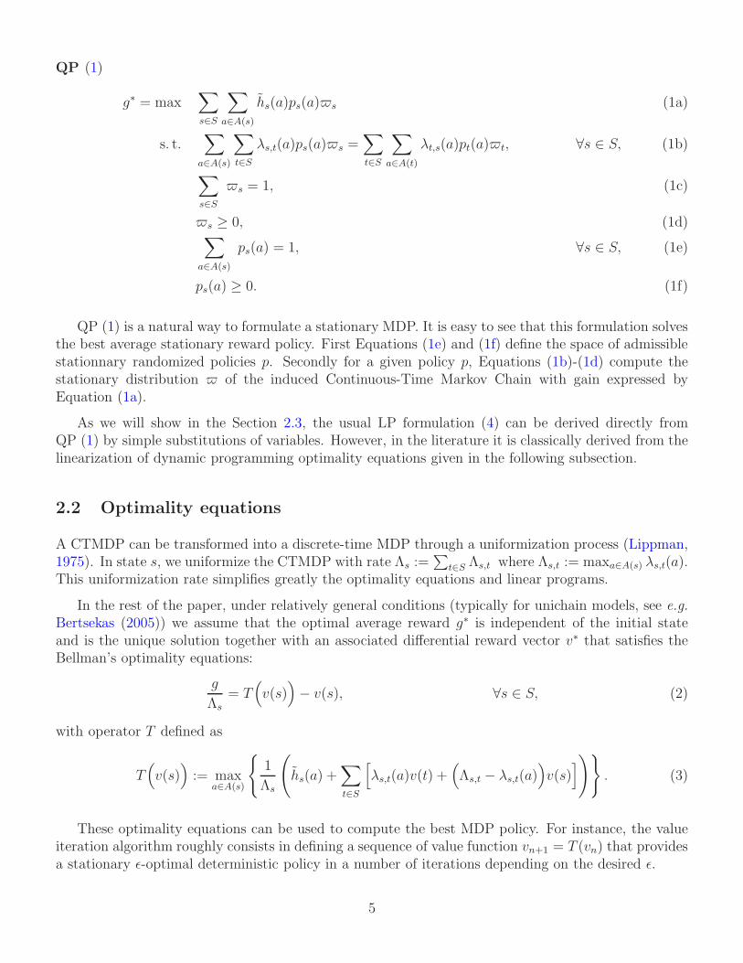
QP (1)

g∗ = max∑

s∈S

∑

a∈A(s)

hs(a)ps(a)s (1a)

s. t.∑

a∈A(s)

∑

t∈S

λs,t(a)ps(a)s =∑

t∈S

∑

a∈A(t)

λt,s(a)pt(a)t, ∀s ∈ S, (1b)

∑

s∈S

s = 1, (1c)

s ≥ 0, (1d)∑

a∈A(s)

ps(a) = 1, ∀s ∈ S, (1e)

ps(a) ≥ 0. (1f)

QP (1) is a natural way to formulate a stationary MDP. It is easy to see that this formulation solvesthe best average stationary reward policy. First Equations (1e) and (1f) define the space of admissiblestationnary randomized policies p. Secondly for a given policy p, Equations (1b)-(1d) compute thestationary distribution of the induced Continuous-Time Markov Chain with gain expressed byEquation (1a).

As we will show in the Section 2.3, the usual LP formulation (4) can be derived directly fromQP (1) by simple substitutions of variables. However, in the literature it is classically derived from thelinearization of dynamic programming optimality equations given in the following subsection.

2.2 Optimality equations

A CTMDP can be transformed into a discrete-time MDP through a uniformization process (Lippman,1975). In state s, we uniformize the CTMDP with rate Λs :=

∑t∈S Λs,t where Λs,t := maxa∈A(s) λs,t(a).

This uniformization rate simplifies greatly the optimality equations and linear programs.

In the rest of the paper, under relatively general conditions (typically for unichain models, see e.g.Bertsekas (2005)) we assume that the optimal average reward g∗ is independent of the initial stateand is the unique solution together with an associated differential reward vector v∗ that satisfies theBellman’s optimality equations:

g

Λs= T

(v(s)

)− v(s), ∀s ∈ S, (2)

with operator T defined as

T(v(s)

):= max

a∈A(s)

{1

Λs

(hs(a) +

∑

t∈S

[λs,t(a)v(t) +

(Λs,t − λs,t(a)

)v(s)

])}. (3)

These optimality equations can be used to compute the best MDP policy. For instance, the valueiteration algorithm roughly consists in defining a sequence of value function vn+1 = T (vn) that providesa stationary ǫ-optimal deterministic policy in a number of iterations depending on the desired ǫ.

5

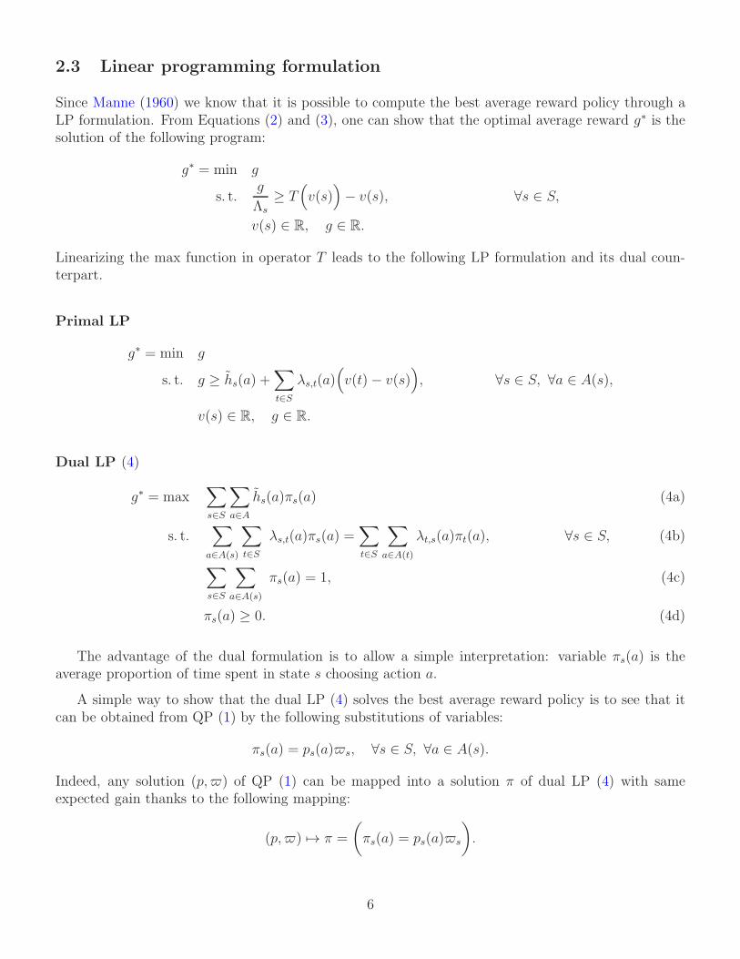
2.3 Linear programming formulation

Since Manne (1960) we know that it is possible to compute the best average reward policy through aLP formulation. From Equations (2) and (3), one can show that the optimal average reward g∗ is thesolution of the following program:

g∗ = min g

s. t.g

Λs≥ T

(v(s)

)− v(s), ∀s ∈ S,

v(s) ∈ R, g ∈ R.

Linearizing the max function in operator T leads to the following LP formulation and its dual coun-terpart.

Primal LP

g∗ = min g

s. t. g ≥ hs(a) +∑

t∈S

λs,t(a)(v(t)− v(s)

), ∀s ∈ S, ∀a ∈ A(s),

v(s) ∈ R, g ∈ R.

Dual LP (4)

g∗ = max∑

s∈S

∑

a∈A

hs(a)πs(a) (4a)

s. t.∑

a∈A(s)

∑

t∈S

λs,t(a)πs(a) =∑

t∈S

∑

a∈A(t)

λt,s(a)πt(a), ∀s ∈ S, (4b)

∑

s∈S

∑

a∈A(s)

πs(a) = 1, (4c)

πs(a) ≥ 0. (4d)

The advantage of the dual formulation is to allow a simple interpretation: variable πs(a) is theaverage proportion of time spent in state s choosing action a.

A simple way to show that the dual LP (4) solves the best average reward policy is to see that itcan be obtained from QP (1) by the following substitutions of variables:

πs(a) = ps(a)s, ∀s ∈ S, ∀a ∈ A(s).

Indeed, any solution (p,) of QP (1) can be mapped into a solution π of dual LP (4) with sameexpected gain thanks to the following mapping:

(p,) 7→ π =

(πs(a) = ps(a)s

).

6

For the opposite direction, there exists several “equivalent” mappings preserving the gain. Theirdifferences lie in the decisions taken in unreachable states (s = 0). We exhibit one:

π 7→ (p,) =

ps(a) =

πs(a)s

, if s 6= 0

1, if s = 0 and a = a1

0, otherwise

, s =

∑

a∈A(s)

πs(a)

.

Since any solution of QP (1) can be mapped to a solution of dual LP (4) and conversely, in thesequel we overload the word policy as follows:

• We (abusively) call (randomized) policy a solution π of the dual LP (4).

• We say that π is a deterministic policy if it satisfies πs(a) ∈ {0, s =∑

a∈A(s) πs(a)}, ∀s ∈

S, ∀a ∈ A(s).

3 Action Decomposed Continuous-TimeMarkov Decision Pro-

cesses

3.1 Definition

An action Decomposed CTMDP (D-CTMDP) is a CTMDP such that:

• In each state s ∈ S, the action space can be written as the Cartesian product of ns ≥ 1 sub-action sets: A(s) = A1(s)× . . .×Ans

(s). An action a ∈ A(s) is then composed by ns sub-actions(a1, . . . , ans

) where ai ∈ Ai(s).

• Sub-action ai increases the transition rate from s to t by λis,t(ai), the reward rate by hi

s(ai) andthe instant reward rate by ris,t(ai).

– The resulting transition rate from s to t is then λs,t(a) =∑ns

i=1 λis,t(ai).

– The resulting aggregated reward rate in state s when action a is taken is then hs(a) =∑ns

i=1 his(ai) with hi

s(ai) = hs(ai) +∑

t∈S λis,t(ai)r

is,t(ai).

D-CTMDPs typically model queueing control problems with several types of events (demand ar-rival, service end, failure, etc), an action associated to each type of event (admission control, routing,repairing, etc) and also a cost associated to each type of event. Event-based DP, as defined by Koole(1998), is included in the class of D-CTMDPs.

For ease of notation, we assume without loss of generality that each state s ∈ S has exactly ns = nindependent sub-action sets, with I = {1, · · · , n}, and that each sub-action set Ai(s) contains exactlyk sub-actions.

We introduce the concept of decomposed policy.

• A (randomized) decomposed policy is a vector p = ((p1s, . . . , pns ), s ∈ S) such that for each state s

there is a probability pis(ai) to select sub-action ai ∈ Ai(s) with∑

ai∈Ai(s)pis(ai) = 1, ∀s ∈ S, ∀i ∈

I. The probability to choose action a = (a1, · · · , an) in state s is then ps(a) =∏

i∈I pis(ai).

7

• A decomposed policy p is said deterministic if ∀s ∈ S, ∀i ∈ I, ∃ai ∈ Ai(s) such that pis(ai) = 1and ∀bi ∈ Ai(s) \ {ai}, pis(bi) = 0. In other words, p selects one sub-action for each state s andeach sub-action set Ai.

In the following we will see that decomposed policies are dominant for D-CTMDPs. It is interestingsince a decomposed policy p is described in a much more compact way than a classic policy p.

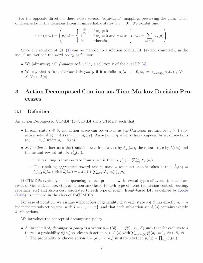
Simply applying the definition, one can check that the best average reward decomposed policy p∗ issolution of the following quadratic program where ˚s is to be interpreted as the stationary distributionof state s ∈ S.

Decomposed QP (5)

g∗ = max∑

s∈S

∑

i∈I

∑

ai∈Ai(s)

his(ai)p

is(ai)˚s (5a)

s. t.∑

i∈I

∑

ai∈Ai(s)

∑

t∈S

λis,t(ai)p

is(ai)˚s =

∑

t∈S

∑

i∈I

∑

ai∈Ai(t)

λit,s(ai)p

it(ai)˚t, ∀s ∈ S, (5b)

∑

s∈S

˚s = 1, (5c)

˚s ≥ 0, (5d)∑

ai∈Ai(s)

pis(ai) = 1, ∀s ∈ S, ∀i ∈ I, (5e)

pis(ai) ≥ 0. (5f)

Example – Dynamic pricing in a multi-class M/M/1 queue (D-CTMDP formulation). Wecontinue the example started in the Section 1. This problem can be modeled as a D-CTMDP with statespace S = {(s1, . . . , sn) | si ≤ C, ∀i ∈ I}. In each state s ∈ S, there is ns = (n+1) sub-actions and anaction can be written as a = (r1, . . . , rn, d) with ri the price decided to be offered to client class i and dthe client class to process. The action space is then A = P n×D with D = {1, . . . , n}. The waiting costin state (s1, . . . , sn) is independent of the action selected and is worth

∑i h

isi. The reward rate incurredby sub-action ri is λi(ri)r

i. Let the function 1b equals 1 if boolean expression b is worth true and 0otherwise. The resulting aggregated reward rate in state s = (s1, . . . , sn) when action a = (r1, . . . , rn, d)is selected is then hs(a) =

∑ni=1 h

is(ri) with hi

s(ri) = hisi + 1si<Cλi(ri)ri.

For this example, the cardinality of the state space and the action space are respectively |S| = (C+1)n

and |A| = knn.

3.2 Optimality equations

Optimality equations for CTMDPs can be rewritten in the context of a D-CTMDPs to take advantageof decomposition properties. Let Λi

s,t = maxai∈Ai(s) λis,t(ai). The uniformization rate is again Λs =∑

t∈S Λs,t where Λs,t, as defined previous section, can be rewritten as follows:

Λs,t = maxa∈A(s)

λs,t(a) = max(a1, ..., an)

∈ A1(s)×...×An(s)

∑

i∈I

λis,t(ai) =

∑

i∈I

maxai∈Ai(s)

λis,t(ai) =

∑

i∈I

Λis,t.

8

Operator T as defined in Equation (3) can be rewritten as:

T(v(s)

)= max

(a1, ..., an)∈ A1(s)×...×An(s)

{1

Λs

∑

i∈I

(his(ai) +

∑

t∈S

[λis,t(ai)v(t) +

(Λi

s,t − λis,t(ai)

)v(s)

])}. (6)

That we can decompose as:

T(v(s)

)=

1

Λs

∑

i∈I

(max

ai∈Ai(s)

{his(ai) +

∑

t∈S

[λis,t(ai)v(t) +

(Λi

s,t − λis,t(ai)

)v(s)

]}). (7)

The value iteration algorithm is much more efficient if T is expressed as in the latter equation.Experimental results presented in Section 5 show it clearly. Indeed computing the maximum requiresnk evaluations in Equation (6) and nk in Equation (7). To the best of our knowledge, this decompositionproperty of operator T is used in many queueing control problems (see Koole (1998) and related papers)but has not been formalized as generally as in this paper.

Example – Dynamic pricing in a multi-class M/M/1 queue (DP approach). We can nowwrite down the optimality equations. We use the following uniformization: let Λ =

∑i∈I Λ

i +∆ withΛi = maxri∈P{λ

i(ri)} and ∆ = maxi∈I {µi}.

For a state s = (s1, . . . , sn) and with ei the unitvector of the ith coordinate, the operator T forclassic optimality equations can be defined as follows:

T

(v(s)

)= max

(r1,...,rn,d)∈A

{∑

i∈I

[hi(ri) + 1si<Cλ

i(ri)v(s+ ei)]

+1sd>0µdv(s− ed) +

(Λ−

∑

i∈I

1si<Cλi(ri) + ∆− 1sd>0µ

d

)v(s)

}.

Since we are dealing with a D-CTMDP, operator T can also be decomposed as:

T

(v(s)

)=

1

Λ

∑

i∈I

hi(ri) + max

ri∈Psi<C

{λi(ri)v(s+ ei) +

(Λi − λi(ri)

)v(s)

}

+maxd∈Dsd>0

{µdv(s− ed) + (∆− µd)v(s)

}).

3.3 LP formulation

Let πis(ai) be interpreted as the average proportion of time spent in state s choosing action ai ∈ Ai(s)

among all sub-actions Ai(s). From decomposed QP (5) we can build the LP (8) formulation withsimple substitutions of variable:

πis(ai) = πi

s(ai)˚s, ∀s ∈ S, ∀i ∈ I, ∀ai ∈ Ai(s).

We obtain that g∗ is the solution of the following LP formulation:

9

Decomposed Dual LP (8)

g∗ = max∑

s∈S

∑

i∈I

∑

ai∈Ai(s)

his(ai)π

is(ai) (8a)

s. t.∑

i∈I

∑

ai∈Ai(s)

∑

t∈S

λis,t(ai)π

is(ai) =

∑

t∈S

∑

i∈I

∑

ai∈Ai(t)

λit,s(ai)π

it(ai), ∀s ∈ S, (8b)

∑

ai∈Ai(s)

πis(ai) = ˚s, ∀s ∈ S, ∀i ∈ I, (8c)

∑

s∈S

˚s = 1, (8d)

πis(ai) ≥ 0, ˚s ≥ 0. (8e)

The decomposed dual LP formulation (8) has |S|(kn + 1) variables and |S|((k + 1)n + 2) + 1constraints. It is much less than the classic dual LP formulation (4) that has |S|kn variables and|S|(kn + 1) constraints.

Lemma 1. Any solution (p, ˚) of decomposed QP (1) can be mapped into a solution (π, ˚) of decom-posed dual LP (4) with same expected gain thanks to the following mapping:

(p, ˚) → (π, ˚) =

(πis(ai) = πi

s(ai)˚s, ˚

).

For the opposite direction, there exists several “equivalent” mappings preserving the gain. Theirdifferences lie in the decisions taken in unreachable states (s = 0). We exhibit one:

(π, ˚) 7→ (p, ˚) =

pis(ai) =

πis(ai)˚s

, if ˚s 6= 0

1, if ˚s = 0 and ai = a10, otherwise

, ˚

.

�

Since any solution of the decomposed QP (5) can be matched to a solution of decomposed dualLP (8) and conversely (Lemma 1), in the sequel we again overload the word policy as follows:

• We (abusively) call (randomized) decomposed policy a solution (˚, π) of the decomposed dualLP (8).

• We say that (˚, π) is a deterministic policy if it satisfies πis(ai) ∈ {0, ˚s}, ∀s ∈ S, ∀i ∈ I, ∀ai ∈

Ai(s).

Dualizing the decomposed dual LP (8), we obtain the following primal version:

10

Decomposed Primal LP (9)

g∗ = min g

s. t. m(s, i) ≥ his(ai) +

∑

t∈S

λis,t(ai)

(v(t)− v(s)

), ∀s ∈ S, ∀i ∈ I, ∀ai ∈ Ai(s),

g ≥∑

i∈I

m(s, i), ∀s ∈ S,

m(s, i) ∈ R, v(s) ∈ R, g ∈ R.

Note that the decomposed primal LP (9) could have also been obtained using the optimalityequations (7). Indeed, under some general conditions (Bertsekas, 2005), the optimal average rewardg∗ is independent from the initial state and together with an associated differential cost vector v∗

it satisfies the optimality equations (7). The optimal average reward g∗ is hence the solution of thefollowing equations:

g∗ = min g

s. t.g

Λs

≥ T(v(s)

)− v(s), ∀s ∈ S.

That can be reformulated using decomposability to have:

g∗ = maxs∈S

{Λs

(T (v(s))− v(s)

)}

= maxs∈S

{∑

i∈I

(max

ai∈Ai(s)

{his(ai) +

∑

t∈S

[λis,t(ai)v(t) +

(Λi

s,t − λis,t(ai)

)v(s)

]− Λi

sv(s)

})}

= maxs∈S

{∑

i∈I

(max

ai∈Ai(s)

{his(ai) +

∑

t∈S

λis,t(ai)

(v(t)− v(s)

)})}. (10)

The LP (9) can be obtained from Equation (10) using Lemma 3 given in appendix.

Example – Dynamic pricing in a multi-class M/M/1 queue (LP approach). With a = (r1, . . . , rn, d) ∈A, we can now formulate its classic dual LP formulation:

max∑

s∈S

∑

a∈A

(n∑

i=1

hi(ri)

)πs(a)

s.t.∑

a∈A

(1sd>0µ

d +n∑

i=1

1si<Cλi(ri)

)πs(a)

=∑

a∈A

(n∑

i=1

1si>0λi(ri)πs−ei(a) + 1sd<Cµ

dπs+ed(a)

), ∀s ∈ S,

∑

s∈S

∑

a∈A

πs(a) = 1,

πs(a) ≥ 0.

11

And its decomposed Dual LP formulation:

max∑

s∈S

n∑

i=1

hi(ri)πis(ri)

s.t. =∑

i∈I

∑

ri∈P

1si>0λi(ri)π

is−ei

(ri) +∑

d∈D

1sd<Cµdπs+ed(d), ∀s ∈ S,

∑

ri∈P

πis(ri) = ˚s, ∀s ∈ S, ∀i ∈ I,

∑

d∈D

πs(d) = ˚s, ∀s ∈ S,

∑

s∈S

˚s = 1,

πis(ri) ≥ 0, πs(d) ≥ 0, ˚s ≥ 0.

3.4 Polyhedral results

Seeing the decomposed dual LP (8) as a reformulation of the decomposed QP (5), see Lemma 1, it isclear that it gives a policy maximizing the average reward. However, it doesn’t provide any structureof optimal solutions. For this purpose, Lemma 2 gives two mappings linking classic and decomposedpolicies that are used in Theorem 1 to prove polyhedral results showing the dominance of deterministicpolicies. This means that the simplex algorithm on the decomposed dual LP (8) will return the bestaverage reward deterministic policy.

Lemma 2. Let a(i) be the ith coordinate of vector a. The following policy mappings preserve thestrictly randomized and deterministic properties:

D : p 7→ p =

pis(ai) =∑

a∈A(s)/a(i)=ai

ps(a)

; D−1 : p 7→ p =

(ps(a1, . . . , an) =

∏

i∈I

pis(ai)

).

Moreover:(a) D is linear.(b) The following policy transformations preserve moreover the excepted gain:

1. (p,) 7→ (p, ˚) = (D(p), );

2. π 7→ (π, ˚) = (D(π), ˚s =∑

a∈A(s) πs(a));

3. (p, ˚) 7→ (p,) = (D−1(p), ˚);

4. (π, ˚) 7→ (π,) = (D−1(π), ˚).

�

Theorem 1. The best decomposed CTMDP average reward policy is solution of the decomposed dualLP (8). Equations (8b)-(8e) describe the convex hull of deterministic policies.

12

Proof: We call P the polytope defined by constraints (8b)-(8e). From Lemma 1 we know that allpolicies are in P . To prove that vertices of P are deterministic policies we use the characterizationthat a vertex of a polytope is the unique optimal solution for some objective.

Assume that (π, ˚) is a strictly randomized decomposed policy, optimal solution with gain g ofthe decomposed dual LP (8) for some objective ho. From Lemma 2 we know that there exists astrictly randomized non decomposed policy (π,) with same expected gain. Deterministic policies aredominant in non decomposed models, therefore there exists a deterministic policy (π∗, ∗) with gaing∗ ≥ g. From Lemma 2 we can convert (π∗, ∗) into a deterministic decomposed policy (π∗, ˚∗) withsame expected gain g∗ = g∗ ≥ g. Since (π, ˚) is optimal we have then g∗ = g∗ which means that (π, ˚)is not the unique optimal solution for objective ho. Therefore a strictly decomposed randomized policycan’t be a vertex of the decomposed LP (8) and P is the convex hull of deterministic policies. �

3.5 Benefits of decomposed LP

First, recall that with the use of action decomposability, decomposed LP (8) allows to have a complexitypolynomial in the number of independent sub-action sets: |S|(kn+ 1) variables and |S|((k + 1)n+ 2)constraints for the dual whereas in the classic it grows exponentially: |S|kn variables and |S|(kn + 1)constraints. In the Section 5 we will see that it has a substantial impact on the computation time.

Secondly, even if the LP (8) is slower to solve than DP (7), as shown experimentally in the Section 5,this mathematical programming approach offers some advantages. First, LP formulations can help tocharacterize the polyhedral structure of discrete optimization problems, see Buyuktahtakin (2011).Secondly, there is in the LP literature generic methods directly applicable such as sensitive analysis,see Filippi (2011), or approximate linear programming techniques, see Dos Santos Eleutrio (2009).Another interesting advantage is that the dual LP (8) is really simple to write and does not need theuniformization necessary to the DP (7) which is sometimes source of waste of time and errors.

Finally, a big benefit of the LP formulation is the ability to add extra constraints that are notknown possible to consider in the DP. A classic constraint that is known possible to add only in theLP formulation is to restrain the stationary distribution on a subset T ⊂ S of states to be greater thana parameter q, for instance to force a quality of service:

∑

s∈T

s ≥ q.

Nevertheless, we have to be aware that such constraint can enforce strictly randomized policies as opti-mal solutions. In the next section we discuss constraints that preserve the dominance of deterministicpolicies.

4 Using decomposed LP to tackle a wider class of large action

space MDP

4.1 Constraining action space, preserving decomposability

In decomposed models we can lose hand on certain action incompatibilities we had on classic ones:

13

Example – Dynamic pricing in a multi-class M/M/1 queue (Adding extra constraints). Let saywe have two prices high h and low l for the n classes of clients. In a state s we have then the followingset of actions: A(s) = P (s) × D(s) where P (s) =

∏ni=1 Pi(s) and Pi(s) = {hi, li}. Assume that, for

some marketing reasons, there needs to be at least one low price selected. In the non decomposed model,it is easily expressible by a new space of action P ′(s) = P (s)\{(h1, . . . , hn)} removing the action whereall high prices are selected. However, it is not possible to use decomposition anymore with this newaction space, even though there is still some structure in the problem.

When reducing the action space event-based DP techniques are inapplicable, but we can use somepolyhedral properties of the LP formulation to model this action space reduction. In Theorem 2, we willshow that it is possible to reduce the action space of any state s ∈ S to A′(s) ⊆ A(s) and to preservethe action decomposability advantage by adding a set of constraints to the decomposed dual LP (8).However, this theorem is not constructive and only proves the existence of such constraints. Moreover,in general the number of constraints necessary to characterize the admissible decomposed policiesmight be exponential and it would be finally less efficient than considering the non decomposed model(Proposition 1). Nevertheless, in some particular cases, one might be able to intuitively formulate somevalid constraints that a decomposed policy should respect as in the following example.

Example – Dynamic pricing in a multi-class M/M/1 queue (Constraining in average). Inaverage we can forbid solutions with all high prices (sub-action hi) by selecting at most n − 1 highprices (Equation (11a)), or at least one low price (sub-action li, Equation (11b)):

n∑

i=1

pis(hi) =

n∑

i=1

πis(hi)

˚s≤ n− 1, (11a)

orn∑

i=1

pis(li) =

n∑

i=1

πis(li)

˚s≥ 1. (11b)

These equations constrain the average behaviour of the system. However, together with decomposeddual LP (8) it is not obvious that they provide optimal deterministic policies in general. In Corollary 1,we will provide a state-policy decomposition criteria to verify if a set of constraints correctly modelsan action space reduction. However, to apply it in general as we will prove in Proposition 2, it involvesto solve a co-NP complete problem. Moreover, when trying to formulate valid constraints, we willsee in Proposition 3 that it is even NP-complete to check whether or not there exists one feasibledeterministic policy (not only the optimal).

These results hold in general, in practice Equations (11a) or (11b) correctly models the actionspace reduction and can be generalized under the general action reduction constraint framework. InCorollary 2 we will prove that we can use several action reduction constraints at the same time (undersome assumptions) and always obtain deterministic policies as optimum. In other words, adding suchconstraints to the decomposed dual LP (8) and using the simplex algorithm to solve it will returnan optimal deterministic solution. Next example provides another application of action reductionconstraint framework.

Example – Dynamic pricing in a multi-class M/M/1 queue (Another extra constraints). Wewant now to select exactly n/2 high prices, the number of actions to remove from the original actionspace is exponential in n: A′(s) = {(a1, . . . , an) |

∑ni=1 1ai=l = n/2} = A(s)\{(a1, . . . , an) |

∑ni=1 1ai=l 6=

14

n/2}. Although, there is a simple way to model this constraint in average with the action reduction con-straint framework ensuring the dominance of deterministic policies:

n∑

i=1

pis(hi) =n∑

i=1

πis(hi)

˚s

=n

2. (12)

4.2 State policy decomposition criteria

In the following for each s ∈ S, πs (resp. ps) represents the matrix of variables πis(ai) (resp. pis(ai))

with i ∈ I and ai ∈ Ai(s). The next theorem states that there exists a set of constraints to add tothe decomposed dual LP (8) so that it correctly solves the policy within A′ maximizing the averagereward criterion and that the maximum is attained by a deterministic policy.

Theorem 2. For a decomposed CTMDP with a reduced action space A′(s) ⊆ A(s), ∀s ∈ S, thereexists a set of linear constraint {Bsps ≤ bs, ∀s ∈ S} that describes the convex hull of deterministicdecomposed policies p in A′(s). Then {Bsπs ≤ bs˚s, ∀s ∈ S} together with equations (8b)-(8e) definesthe convex hull of decomposed deterministic policies (π, ˚) in A′.

Proof: Equations (1e) and (1f) of non decomposed QP (1) specify the space of feasible policies pfor a classic CTMDP. For each state s ∈ S we can reformulate this space by the convex hull of allfeasible deterministic policies: ps ∈ conv{ps | ∃a ∈ A′(s) s.t. ps(a) = 1}. We use the mappings D andD−1 defined in Lemma 2. Note that for any linear mapping M and any finite set X , conv(M(X)) =M(conv(X)). D is linear, therefore for each state s ∈ S the convex hull Hs of CTMDPs policy withsupports in A′(s) is mapped into the convex hull Hs of decomposed CTMDPs state policy in A′(s):

D(Hs) = Hs

⇔ D

(conv

{ps | ∃a ∈ A′(s) s.t. ps(a) = 1

})= conv

{D(ps) | ∃a ∈ A′(s) s.t. ps(a) = 1

}

= conv

{ps | ∃(a1, . . . , an) ∈ A′(s) s.t. pis(ai) = 1

}.

Recall (a particular case of) Minkowski-Weyl’s theorem: for any finite set of vectors A′ ⊆ Rn there

exists a finite set of linear constraints {Bv ≤ b} that describes the convex hull of vectors v in A′. Hs

is convex hence from Minkowski-Weyl’s theorem there exists a matrix Bs and a vector bs such thatvectors ps in Hs can be described by the constraints Bsps ≤ bs. In the decomposed dual QP (5) we canthen replace Equations (5e) and (5f) that specify the set of feasible D-CTMDP policies by constraints{Bsps ≤ bs, ∀s ∈ S}. With substitutions of variable, constraints C := {Bsπs ≤ bs˚s, ∀s ∈ S} arelinear in (πs, ˚s) and can hence be added to the decomposed dual LP (8).

As in Theorem 1, with the characterization that a vertex of a polytope is the unique solution forsome objective, we prove now that the vertices of the polytope defined by Equations (8b)-(8e) togetherwith constraints C are deterministic policies. Assume (π, ˚) is a strictly randomized decomposedpolicy of gain g, optimal solution of the decomposed dual LP (8) for some objective h0 together withconstraints C. (π, ˚) can be mapped into a strictly randomized non decomposed policy (π,), stillrespecting C, with same expected gain that is dominated by a deterministic policy (π∗, ∗) respectingalso C with gain g∗ ≥ g. (π∗, ∗) can be again mapped into a deterministic decomposed policy

15

(π∗, ˚∗) respecting C with same expected gain g∗ = g∗ ≥ g. But since (π, ˚) is optimal we have theng∗ = g∗ which means that (π, ˚) is not the unique optimal solution for objective h0. Therefore, astrictly decomposed randomized policy can’t be a vertex of the decomposed dual LP (8) together withconstraints C. �

Corollary 1 (State policy decomposition criteria). If the vertices of the polytope {Bsps ≤ bs} are {0, 1}-vectors for each state s ∈ S, decomposed dual LP (8) together with constraints {Bsπs ≤ bs˚s, ∀s ∈ S}has a deterministic decomposed policies as optimum solution.

In other words, if in any states s ∈ S, one finds a set of constraints {Bsps ≤ bs} defining a {0, 1}-polytope constraining in average the feasible policies p to be in the reduced action space A′(s), then,the state policy decomposition criteria of Corollary 1 says that solving the decomposed dual LP (8)together with constraints {Bsπs ≤ bs˚s, ∀s ∈ S} will provide an optimal deterministic policy in A′.

4.3 Complexity and efficiency of action space reduction

We return to our example in the Section 4.1, where we want to use action decomposability on a reducedaction space A′(s) = D(s) ×

∏ni=1 Pi(s) \ {(h1, . . . , hn)}. Theorem 2 states that there exists a set of

constraints to add in the decomposed dual LP (8) such that it will return the best policies within A′

and that this policy will be deterministic. However, as we show in the next proposition, in general thepolyhedral description of a subset of decomposed policies can be less efficient than the non-decomposedones.

Proposition 1. The number of constraints necessary to describe a subset of decomposed policies canbe higher than the number of corresponding non-decomposed policies itself.

Proof: There is a positive constant c such that there exist {0, 1}-polytopes in dimension n with( cnlogn

)n4 facets (Barany and Por, 2001), while the number of vertices is less than 2n. �

In practice, we saw in our dynamic pricing example that one can formulate valid inequalities. Wecan apply Corollary 1 to check if the decomposed dual LP (8) together with equations (11b) correctlymodels the action space reduction. However, to use Corollary 1 we would need to be able to checkif these constraints define a polytope with {0, 1}-vector vertices. In general, to determine whether apolyhedron {x ∈ R

n : Ax ≤ b} is integral is co-NP-complete (Papadimitriou and Yannakakis, 1990).In the next proposition we show that it is also co-NP-complete for {0 − 1}-polytopes as a directconsequence of Ding et al. (2008).

Proposition 2. Determining whether a polyhedron {x ∈ [0, 1]n : Ax ≤ b} is integral is co-NP-complete.

Proof: Let A′ be a {0 − 1}-matrix with precisely two ones in each column. From Ding et al.(2008) we know that the problem of deciding whether the polyedron P defined by the linear system{A′x ≥ 1, x ≥ 0} is integral is co-NP-complete. Note that all vertices v of P respect 0 ≤ v ≤ 1.Therefore, {A′x ≥ 1, x ≥ 0} is integral if and only if {A′x ≥ 1, 0 ≤ x ≤ 1} is integral. It means thatdetermining whether the polyedron P defined by the linear system {A′x ≥ 1, 0 ≤ x ≤ 1} is integral isco-NP-complete. This is a particular case of determining whether for a general matrix A a polyhedron{x ∈ [0, 1]n : Ax ≤ b} is integral. �

16

As a consequence of Proposition 2, deciding if {Bsps ≤ bs, ∀s ∈ S} defines the convex hull ofdeterministic policies it contains is co-NP-complete. In fact, it is even NP-complete to determine if itcontains a deterministic policy solution at all:

Proposition 3. Consider a decomposed CTMDP with extra constraints of the form {Bsps ≤ bs, ∀s ∈S}. Determining if there exists a feasible deterministic policy solution of this decomposed CTMDP isNP-complete even if |S| = 1.

Proof: We show a reduction to the well known NP-complete problem 3-SAT. We reduce a 3-SATinstance with a set V of n variables and m clauses to a D-CTMDP instance. The system is composedwith only one state s, so s = 1. Each variable v creates an independent sub-action set Av containingtwo sub-actions representing the two possible states (literal l) of the variable: v and v. We have thenA =

∏v∈V Av =

∏v∈V {v, v} . Each clause C generates a constraint:

∑l∈C l ≥ 1. Finally, there exists a

deterministic feasible policy for the D-CTMDP instance if and only if the 3-SAT instance is satisfiable.�

4.4 An interesting generic constraint

Definition 1 (Action reduction constraint). An action reduction constraint (s, R,m,M) constrain ina state s ∈ S to select in average at least m and at most M sub-actions ai out of a set R belonging todifferent sub-action sets Ai(s). Its feasible policies space is defined by the following equation:

m ≤∑

ai∈R

pis(ai) =∑

ai∈R

πis(ai)

˚s≤ M. (13)

Although it is hard in general to find and to prove that a given set of linear equations modelscorrectly a reduced action space, we show in the following corollary, consequence of Corollary 1, thatit is nevertheless possible to exhibit some valid constraints.

Corollary 2. Combination of action reduction constraints] For a set of action reduction constraints{(sj , Rj, mj ,Mj) | j ∈ J}, if no sub-action ai is present in more than one action reduction constraintRj, then the decomposed dual LP (8), together with Equations {(13) | j ∈ J}, preserves the dominanceof optimal policies. Moreover, the solution space of this LP is the convex hull of deterministic policiesrespecting the action reduction constraints. More formally, this sufficient condition can be reformulatedas: ∀s ∈ S,

⋃j∈J Rj is a sub-partition of

⋃i∈I Ai(s).

Proof: We know that pis(ai) =πis(ai)˚s

is the discrete probability to take action ai out of all actionsAi(s) in state s. Therefore, in state s, for an action reduction constraint (s, R,m,M), Equation (13)reduces the solution space to the decomposed randomized policies that select in average at least m andat most M actions out of the set R: m ≤

∑ai∈R

pis(ai) ≤ M .

If no sub-action is present in more than one action reduction constraint, then the matrix {∑

ai∈Rjpis(ai), j ∈

J} is totally unimodular and defines therefore a polytope with {0, 1}-vector vertices. Using Corollary 1we know then that deterministic policies are dominant. �

Returning to our dynamic pricing example where we want to have at least one low price selected.From Corollary 2, we know now that adding Equations (11a) or (11b) to LP (8) will return optimaldeterministic policies with a simplex solution technique. It is also the case when imposing to haveexactly half of the high prices selected with Equations (12).

17

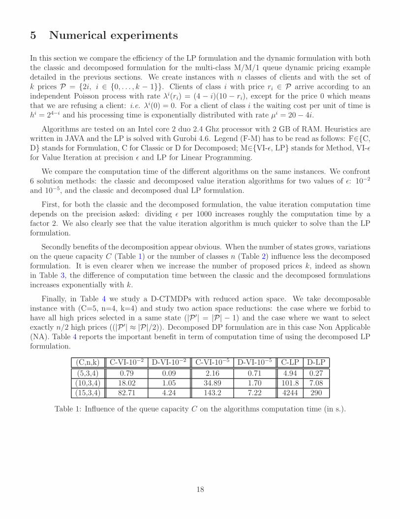
5 Numerical experiments

In this section we compare the efficiency of the LP formulation and the dynamic formulation with boththe classic and decomposed formulation for the multi-class M/M/1 queue dynamic pricing exampledetailed in the previous sections. We create instances with n classes of clients and with the set ofk prices P = {2i, i ∈ {0, . . . , k − 1}}. Clients of class i with price ri ∈ P arrive according to anindependent Poisson process with rate λi(ri) = (4 − i)(10 − ri), except for the price 0 which meansthat we are refusing a client: i.e. λi(0) = 0. For a client of class i the waiting cost per unit of time ishi = 24−i and his processing time is exponentially distributed with rate µi = 20− 4i.

Algorithms are tested on an Intel core 2 duo 2.4 Ghz processor with 2 GB of RAM. Heuristics arewritten in JAVA and the LP is solved with Gurobi 4.6. Legend (F-M) has to be read as follows: F∈{C,D} stands for Formulation, C for Classic or D for Decomposed; M∈{VI-ǫ, LP} stands for Method, VI-ǫfor Value Iteration at precision ǫ and LP for Linear Programming.

We compare the computation time of the different algorithms on the same instances. We confront6 solution methods: the classic and decomposed value iteration algorithms for two values of ǫ: 10−2

and 10−5, and the classic and decomposed dual LP formulation.

First, for both the classic and the decomposed formulation, the value iteration computation timedepends on the precision asked: dividing ǫ per 1000 increases roughly the computation time by afactor 2. We also clearly see that the value iteration algorithm is much quicker to solve than the LPformulation.

Secondly benefits of the decomposition appear obvious. When the number of states grows, variationson the queue capacity C (Table 1) or the number of classes n (Table 2) influence less the decomposedformulation. It is even clearer when we increase the number of proposed prices k, indeed as shownin Table 3, the difference of computation time between the classic and the decomposed formulationsincreases exponentially with k.

Finally, in Table 4 we study a D-CTMDPs with reduced action space. We take decomposableinstance with (C=5, n=4, k=4) and study two action space reductions: the case where we forbid tohave all high prices selected in a same state (|P ′| = |P| − 1) and the case where we want to selectexactly n/2 high prices ((|P ′| ≈ |P|/2)). Decomposed DP formulation are in this case Non Applicable(NA). Table 4 reports the important benefit in term of computation time of using the decomposed LPformulation.

(C,n,k) C-VI-10−2 D-VI-10−2 C-VI-10−5 D-VI-10−5 C-LP D-LP

(5,3,4) 0.79 0.09 2.16 0.71 4.94 0.27(10,3,4) 18.02 1.05 34.89 1.70 101.8 7.08(15,3,4) 82.71 4.24 143.2 7.22 4244 290

Table 1: Influence of the queue capacity C on the algorithms computation time (in s.).

18

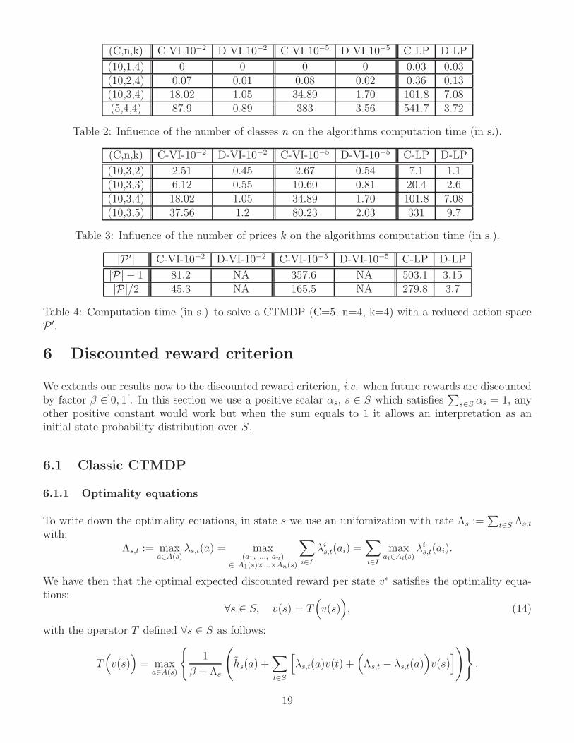
(C,n,k) C-VI-10−2 D-VI-10−2 C-VI-10−5 D-VI-10−5 C-LP D-LP

(10,1,4) 0 0 0 0 0.03 0.03(10,2,4) 0.07 0.01 0.08 0.02 0.36 0.13(10,3,4) 18.02 1.05 34.89 1.70 101.8 7.08(5,4,4) 87.9 0.89 383 3.56 541.7 3.72

Table 2: Influence of the number of classes n on the algorithms computation time (in s.).

(C,n,k) C-VI-10−2 D-VI-10−2 C-VI-10−5 D-VI-10−5 C-LP D-LP

(10,3,2) 2.51 0.45 2.67 0.54 7.1 1.1(10,3,3) 6.12 0.55 10.60 0.81 20.4 2.6(10,3,4) 18.02 1.05 34.89 1.70 101.8 7.08(10,3,5) 37.56 1.2 80.23 2.03 331 9.7

Table 3: Influence of the number of prices k on the algorithms computation time (in s.).

|P ′| C-VI-10−2 D-VI-10−2 C-VI-10−5 D-VI-10−5 C-LP D-LP

|P| − 1 81.2 NA 357.6 NA 503.1 3.15|P|/2 45.3 NA 165.5 NA 279.8 3.7

Table 4: Computation time (in s.) to solve a CTMDP (C=5, n=4, k=4) with a reduced action spaceP ′.

6 Discounted reward criterion

We extends our results now to the discounted reward criterion, i.e. when future rewards are discountedby factor β ∈]0, 1[. In this section we use a positive scalar αs, s ∈ S which satisfies

∑s∈S αs = 1, any

other positive constant would work but when the sum equals to 1 it allows an interpretation as aninitial state probability distribution over S.

6.1 Classic CTMDP

6.1.1 Optimality equations

To write down the optimality equations, in state s we use an unifomization with rate Λs :=∑

t∈S Λs,t

with:Λs,t := max

a∈A(s)λs,t(a) = max

(a1, ..., an)∈ A1(s)×...×An(s)

∑

i∈I

λis,t(ai) =

∑

i∈I

maxai∈Ai(s)

λis,t(ai).

We have then that the optimal expected discounted reward per state v∗ satisfies the optimality equa-tions:

∀s ∈ S, v(s) = T(v(s)

), (14)

with the operator T defined ∀s ∈ S as follows:

T(v(s)

)= max

a∈A(s)

{1

β + Λs

(hs(a) +

∑

t∈S

[λs,t(a)v(t) +

(Λs,t − λs,t(a)

)v(s)

])}.

19

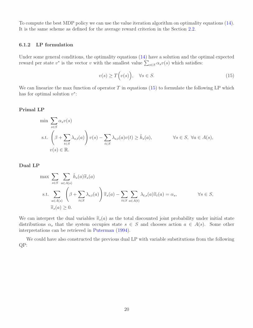
To compute the best MDP policy we can use the value iteration algorithm on optimality equations (14).It is the same scheme as defined for the average reward criterion in the Section 2.2.

6.1.2 LP formulation

Under some general conditions, the optimality equations (14) have a solution and the optimal expectedreward per state v∗ is the vector v with the smallest value

∑s∈S αsv(s) which satisfies:

v(s) ≥ T(v(s)

), ∀s ∈ S. (15)

We can linearize the max function of operator T in equations (15) to formulate the following LP whichhas for optimal solution v∗:

Primal LP

min∑

s∈S

αsv(s)

s.t.

(β +

∑

t∈S

λs,t(a)

)v(s)−

∑

t∈S

λs,t(a)v(t) ≥ hs(a), ∀s ∈ S, ∀a ∈ A(s),

v(s) ∈ R.

Dual LP

max∑

s∈S

∑

a∈A(s)

hs(a)πs(a)

s.t.∑

a∈A(s)

(β +

∑

t∈S

λs,t(a)

)πs(a)−

∑

t∈S

∑

a∈A(t)

λt,s(a)πt(a) = αs, ∀s ∈ S,

πs(a) ≥ 0.

We can interpret the dual variables πs(a) as the total discounted joint probability under initial statedistributions αs that the system occupies state s ∈ S and chooses action a ∈ A(s). Some otherinterpretations can be retrieved in Puterman (1994).

We could have also constructed the previous dual LP with variable substitutions from the followingQP:

20

QP

max∑

s∈S

∑

a∈A(s)

hs(a) ˜ sps(a)

s.t.∑

a∈A(s)

(β +

∑

t∈S

λs,t(a)

)˜ sps(a)−

∑

t∈S

∑

a∈A(t)

λt,s(a) ˜ tpt(a) = αs, ∀s ∈ S,

∑

s∈S

∑

a∈A(s)

ps(a) = 1,

˜ s ≥ 0, ps(a) ≥ 0.

6.2 Action Decomposed CTMDP

6.2.1 Optimality equations

To use the action decomposability we rewrite optimality equations (14) with an explicit decomposition.Using the same uniformization as in the classic case we obtain a decomposed operator T : ∀s ∈ S,

T(v(s)

)= max

(a1, ..., an)∈ A1(s)×...×An(s)

{n∑

i=1

[1

β + Λs

(his(ai) +

∑

t∈S

[λis,t(ai)v(t) +

(Λi

s,t − λis,t(ai)

)v(s)

])]}

=∑

i=∈I

[max

ai∈Ai(s)

{1

β + Λs

(his(ai) +

∑

t∈S

[λis,t(ai)v(t) +

(Λi

s,t − λis,t(ai)

)v(s)

])}].

To compute the best MDP policy we can now use again the value iteration algorithm but with thedecomposed operator that is much more efficient. The optimality equations with the decomposedoperator also lead to a LP formulation that we formulate in the next section.

6.2.2 LP formulation

Under some general conditions, optimality equations (14) with decomposed operator T have a solutionand the optimal expected reward per state v∗ is the vector v with the smallest value

∑s∈S αsv(s) which

satisfies:

αv∗ = min∑

s∈S

αsv(s)

s. t. v(s) ≥ T(v(s)

), ∀s ∈ S.

21

That we can reformulate:

min∑

s∈S

αsv(s)

s. t. 0 ≥ maxs∈S

{T(v(s)

)− v(s)

}

≥ maxs∈S

{(β + Λs)(T

(v(s)

)− v(s))

}

≥ maxs∈S

{n∑

i=1

[max

ai∈Ai(s)

{his(ai) +

∑

t∈S

λis,t(ai)

(v(t)− v(s)

)}]− βv(s)

}.

With Lemma 4 (given in appendix) we obtain that v∗ is the solution of the following LP.

Decomposed Primal LP

min∑

s∈S

αsv(s)

s.t. m(s, i) ≥ his(ai) +

∑

t∈S

λis,t(ai)

(v(t)− v(s)

), ∀s ∈ S, ∀i ∈ I, ∀ai ∈ Ai(s),

βv(s)−∑

i∈I

m(s, i) ≥ 0, ∀s ∈ S ≤ 0,

m(s, i) ∈ R, v(s) ∈ R.

Decomposed Dual LP

max∑

s∈S

∑

i∈I

∑

ai∈Ai(s)

˚πi

s(ai)his(ai)

s.t.∑

ai∈Ai(s)

˚πi

s(ai) =˚

s, ∀s ∈ S, ∀i ∈ I,

β ˚s +∑

i∈I

∑

ai∈Ai(s)

∑

t∈S

λis,t(ai)π

i

s(ai)−∑

t∈S

∑

i∈I

∑

ai∈Ai(t)

λit,s(ai)π

i

t(ai) = αs, ∀s ∈ S,

˚πi

s(ai) ≥ 0, ˚s ≥ 0.

Under initial state distributions α, we can interpret ˚s as the total discounted joint probability that

the system occupies state s ∈ S under initial state distributions αs, and ˚πi

s(ai) as the total discountedjoint probability that the system occupies state s ∈ S and chooses action ai ∈ Ai(s). The decomposeddual LP has |S|(kn + 1) variables and |S|((k + 1)n + 2) constraints. It is much less than the classicdual LP that has |S|kn variables and |S|(kn + 1) constraints.

We could have also constructed the previous dual decomposed LP with variable substitutions fromthe following QP:

22

Decomposed QP

max∑

s∈S

∑

i∈I

∑

ai∈Ai(s)

his(ai)p

is(ai)

˚s

s.t. β ˚s +∑

i∈I

∑

ai∈Ai(s)

∑

t∈S

λis,t(ai)p

is(ai)

˚s −

∑

t∈S

∑

i∈I

∑

ai∈Ai(t)

λit,s(ai)p

it(ai)

˚t = αs, ∀s ∈ S,

∑

ai∈Ai(s)

pis(ai) = 1, ∀s ∈ S, ∀i ∈ I,

pis(ai) ≥ 0, ˚s ≥ 0.

Remark 1. Theorems 1, 2, Propositions 1, 2, 3, Corollary 1 and 2 are also applicable when consideringthe discounted reward criterion with the substitution (π, ˜ ) → (π,), (π, ˚) → (π, ˚) and hence

ps(a) =˚πs(a)˚

sand pis(ai) =

˚πi

s(ai)˚

s.

A From decomposed DP to decomposed LP

The following lemmata help to pass from decomposed optimality DP equations to decomposed LPformulations. For the average reward criterion, using Lemma 3 can build decomposed primal LP (9)from optimality Equations (10). Lemma 3 do the same transformation for the discounted rewardcriterion.

Lemma 3. For any finite sets S, I, A and any data coefficients γs,i,a ∈ R with s ∈ S, i ∈ I anda ∈ A, the value

g∗ = maxs∈S

{∑

i∈I

maxa∈A

{γs,i,a

}}

is the solution of the following LP:

g∗ = min g

s. t. m(s, i) ≥ γs,i,a, ∀s ∈ S, ∀i ∈ I, ∀a ∈ A,

g ≥∑

i∈I

m(s, i), ∀s ∈ S,

m(s, i) ∈ R, ∀s ∈ S, ∀i ∈ I,

g ∈ R.

Proof: Let g∗ be an optimal solution of this LP. First it is trivial that g∗ ≥ maxs∈S{∑

i∈I m(s, i)}and

that Moreover we are minimizing g without any other constraints, hence g∗ = maxs∈S{∑

i∈I m(s, i)}.

Secondly for any optimal solution g∗, there exists s′ ∈ S such that∑

i∈I m(s′, i) = g∗ and ∀i ∈I, m(s′, i) = maxa∈A {γs′,i,a}, otherwise there would exist a strictly better solution. Therefore finallyg∗ = maxs∈S

{∑i∈I maxa∈A {γs,i,a}

}. �

Lemma 4. For any finite sets S, I, A, any data coefficients αs, γs,t,i,a, δs,i,a, ζs ∈ R, s, t ∈ S, i ∈ Iand a ∈ A, the vector v ∈ R

|S| with the smallest value∑

s∈S αsv(s) satisfying

0 ≥ maxs∈S

{∑

i∈I

maxa∈A

{∑

t∈S

γs,t,i,av(s) + δs,i,a

}+ ζsv(s)

}

23

is the solution of the following LP:

min∑

s∈S

αsv(s)

s. t. m(s, i) ≥∑

t∈S

γs,t,i,av(s) + δs,i,a, ∀s ∈ S, ∀i ∈ I, ∀a ∈ A,

0 ≥∑

i∈I

m(s, i) + ζsv(s), ∀s ∈ S,

m(s, i) ∈ R, v(s) ∈ R.

Proof: It is clear that we are minimizing∑

s∈S αsv(s). Now for any vector v we can see that ∀s ∈S, ∀i ∈ I, m(s, i) ≥ maxa∈A

{∑t∈S γs,t,i,av(s) + δs,i,a

}, and we have ∀s ∈ S,

∑i∈I m(s, i) + ζsv(s) ≤ 0.

Therefore any vector v solution must satisfy ∀s ∈ S 0 ≥∑

i∈I maxa∈A{∑

t∈S γs,t,i,av(s) + δs,i,a}+ζsv(s)

and finally 0 ≥ maxs∈S{∑

i∈I maxa∈A{∑

t∈S γs,t,i,av(s) + δs,i,a}+ ζsv(s)

}. �

References

I. Barany and A. Por. On 0-1 polytopes with many facets. Advances in Mathematics, 161(2):209–228,2001.

D. P. Bertsekas. Dynamic programming and optimal control. Vol. II. 3rd ed., Athena Scientific,Belmont, MA, 2005.

D. P. Bertsekas and D. A. Castanon. Adaptive aggregation methods for infinite horizon dynamicprogramming. Automatic Control, IEEE Transactions on, 34(6):589–598, 1989.

I. E. Buyuktahtakin. Dynamic Programming Via Linear Programming. John Wiley &Sons, Inc., 2011. ISBN 9780470400531. doi: 10.1002/9780470400531.eorms0277. URLhttp://dx.doi.org/10.1002/9780470400531.eorms0277.

E. B. Cil, F. Karaesmen, and E. L. Ormeci. Dynamic pricing and scheduling in a multi-class single-server queueing system. Queueing Systems - Theory and Applications, 67:305–331, 2011. doi: 10.1007/s11134-011-9214-5.

G. Ding, L. Feng, and W. Zang. The complexity of recognizing linear systems with certain integralityproperties. Mathematical Programming, Series A, 114:321334, 2008. DOI 10.1007/s10107-007-0103-y.

V. L. Dos Santos Eleutrio. Finding Approximate Solutions for Large Scale Linear Programs. PhDthesis, ETH Zurich, 2009.

C. Filippi. Sensitivity Analysis in Linear Programming. Wiley Encyclopedia of Operations Researchand Management Science, 2011.

X. Guo and O. Hernandez-Lerma. Continuous-Time Markov Decision Processes: Theory and Appli-cations. Stochastic modelling and applied probability. Springer Verlag, 2009. ISBN 9783642025464.URL http://books.google.fr/books?id=tgi-opMlLTwC.

24

Jiaqiao Hu, Michael C Fu, Vahid R Ramezani, and Steven I Marcus. An evolutionary random policysearch algorithm for solving markov decision processes. INFORMS Journal on Computing, 19(2):161–174, 2007.

G. M. Koole. Structural results for the control of queueing systems using event-based dynamic pro-gramming. Queueing Systems, 1998.

C. Li and M. J. Neely. Delay and rate-optimal control in a multi-class priorityqueue with adjustable service rates. In Albert G. Greenberg and Kazem Sohraby,editors, INFOCOM, pages 2976–2980. IEEE, 2012. ISBN 978-1-4673-0773-4. URLhttp://dblp.uni-trier.de/db/conf/infocom/infocom2012.html#LiN12.

S. A. Lippman. Applying a new device in the optimization of exponential queuing systems. OperationResearch, 1975.

C. Maglaras. Revenue management for a multiclass single-server queue via a fluid model analysis.Operations Research, 2006.

A. S. Manne. Linear programming and sequential decisions. Operations Research, 1960.

C. H. Papadimitriou and M. Yannakakis. On recognizing integer polyhedra. Combinatorica, 10(1):107–109, 1990.

M. L. Puterman. Markov Decision Processes: Discrete Stochastic Dynamic Programming. John Wileyand Sons, New York, NY, 1994.

J. N. Tsitsiklis and B. Van Roy. Feature-based methods for large scale dynamic programming. MachineLearning, 22(1):59–94, 1996.

R. Weber and S. Stidham. Optimal control of service rates in networks of queues. Advanced appliedprobabilities, 19:202–218, 1987.

25