Embed Size (px)
Citation preview
Velocity Averaging, Kinetic Formulations,
and Regularizing Effects in Quasi-Linear PDEs
EITAN TADMORUniversity of Maryland, College Park
AND
TERENCE TAOUniversity of California, Los Angeles
To Peter Lax and Louis Nirenberg on their 80th birthdaysWith friendship and admiration
Abstract
We prove in this paper new velocity-averaging results for second-order multi-
dimensional equations of the general form L(∇x , v) f (x, v) = g(x, v) where
L(∇x , v) := a(v) · ∇x − ∇�x · b(v)∇x . These results quantify the Sobolev regu-
larity of the averages,∫v f (x, v)φ(v)dv, in terms of the nondegeneracy of the set
{v : |L(iξ, v)| ≤ δ} and the mere integrability of the data, ( f, g) ∈ (L px,v, Lq
x,v).
Velocity averaging is then used to study the regularizing effect in quasi-linear
second-order equations, L(∇x , ρ)ρ = S(ρ), which use their underlying kinetic
formulations, L(∇x , v)χρ = gS . In particular, we improve previous regularity
statements for nonlinear conservation laws, and we derive completely new regu-
larity results for convection-diffusion and elliptic equations driven by degenerate,
nonisotropic diffusion. c© 2007 Wiley Periodicals, Inc.
1 Introduction
We study the regularity of solutions to multidimensional quasi-linear scalar
equations of the form
(1.1)
d∑j=0
∂
∂xjAj (ρ) −
d∑j,k=1
∂2
∂xj∂xkBjk(ρ) = S(ρ)
where ρ : R1+d → R is the unknown field and Aj , Bjk , and S are given functions
from R to R.
This class of equations governs time-dependent solutions ρ(t = x0, x) of non-
linear conservation laws where A0(ρ) = ρ and Bjk ≡ 0, time-dependent solutions
of degenerate diffusion and convection-diffusion equations where {B ′jk} ≥ 0, and
spatial solutions ρ(x) of degenerate elliptic equations where Aj ≡ 0. The notion
of solution should be interpreted here in an appropriate weak sense, since we focus
our attention on the degenerate diffusion case, which is too weak to enforce the
Communications on Pure and Applied Mathematics, Vol. LX, 1488–1521 (2007)c© 2007 Wiley Periodicals, Inc.
VELOCITY AVERAGING AND REGULARITY OF QUASI-LINEAR PDES 1489
smoothness required for a notion of a strong solution. Instead, a common feature
of such problems is the (limited) regularity of their solutions, which is dictated by
the nonlinearity of the governing equations. A prototype example is provided by
discontinuous solutions of nonlinear conservation laws. In [36], Lions, Perthame,
and Tadmor have shown that entropy solutions of such laws admit a regularizing
effect of a fractional order, dictated by the order of nondegeneracy of the equations.
In this paper we extend this result for the general class of second-order equations
(1.1). In particular, we improve the regularity statement in [36] for nonlinear con-
servation laws, and we derive completely new regularity results for convection-
diffusion and elliptic equations driven by degenerate, nonisotropic diffusion.
The derivation of these regularity results employs a kinetic formulation of (1.1).
To describe this formulation let us proceed formally, seeking an equation that gov-
erns the indicator function associated with ρ, χρ(x)(v) := sgn(v)(|ρ| − |v|)+; it
depends on an auxiliary, so-called velocity variable v ∈ R, borrowing the terminol-
ogy from the classical kinetic framework. To this end, we consider the distribution
g = g(x, v), defined via its velocity derivative ∂vg using the formula
(1.2) ∂vg(x, v) := (a(v) · ∇x − ∇�
x · b(v)∇x + S(v)∂v
)χρ(x)(v),
where the convection vector a and diffusion matrix b are given by aj := A′j and
bjk := B ′jk ≥ 0. Observe that the nonlinear quantities �(ρ) can be expressed as
the v-moments of χρ , �(ρ) ≡ ∫v�′(v)χρ(v)dv, �(0) = 0. Therefore, by velocity
averaging of (1.2), we recover (1.1). Moreover, for a proper notion of weak solution
ρ, one augments (1.1) with additional conditions on the behavior of �(ρ) for a
large enough family of entropies �. These additional entropy conditions imply
that g is in fact a positive distribution g = m ∈ M+ that measures the entropy
dissipation of the nonlinear equation.
We arrive at the kinetic formulation of (1.1)
(1.3) L(∇x , v) f (x, v) = ∂vm − S(v)∂vχρ(x)(v), f = χρ, m ∈ M+,
where L is identified with the linear symbol L(iξ, v) := a(v) · iξ −〈b(v)ξ, ξ〉. We
recall that ρ(x) itself can be recovered by velocity averaging of f (x, v) = χρ(v)
via the identity ρ(x) = ∫f (x, v)dv. In Section 2 we discuss the regularity gained
by such velocity averaging.
There is a relatively short yet intense history of such regularity results, com-
monly known as “velocity-averaging lemmas.” We mention the early works of
[20, 24] and their applications, in the context of nonlinear conservation laws, in
[29, 35, 36, 37]; a detailed list of references can be found in [39] and is revisited
in Section 2 below. Almost all previous averaging results dealing with (1.3) are
restricted to the first-order transport equation, degL(iξ, · ) = 1. In Section 2.2
we present an extension to general symbols L that satisfy the so-called truncationproperty; luckily, as shown in Section 2.4 below, all L with degL(iξ, · ) ≤ 2 sat-
isfy this property. If L satisfies the truncation property and it is nondegenerate in
1490 E. TADMOR AND T. TAO
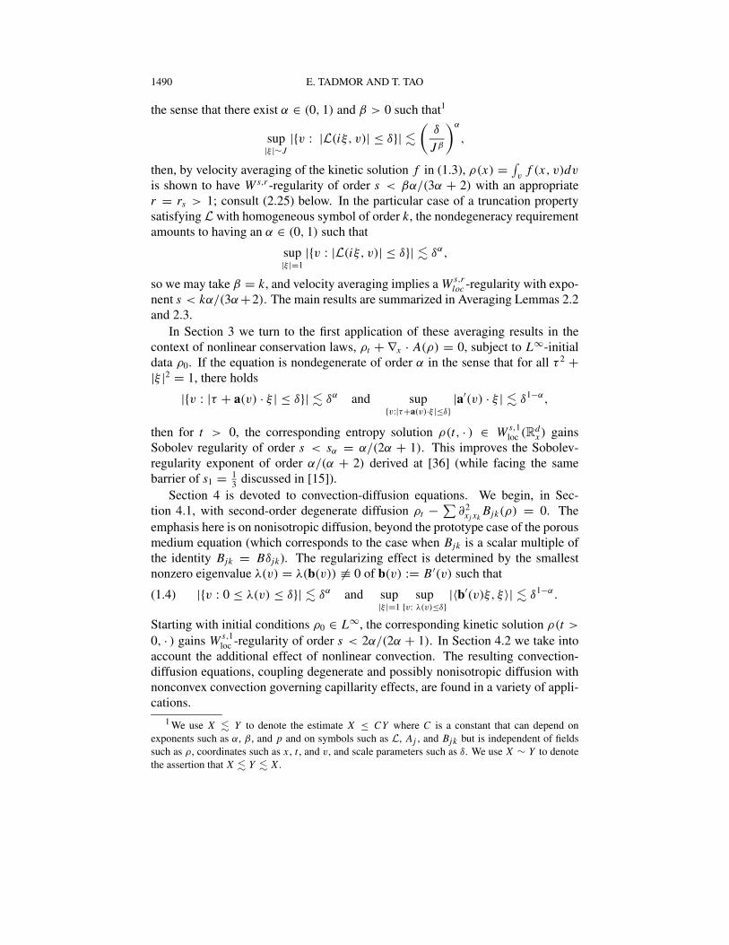
the sense that there exist α ∈ (0, 1) and β > 0 such that1
sup|ξ |∼J
|{v : |L(iξ, v)| ≤ δ}| �
(δ
J β
)α
,
then, by velocity averaging of the kinetic solution f in (1.3), ρ(x) = ∫v
f (x, v)dv
is shown to have W s,r -regularity of order s < βα/(3α + 2) with an appropriate
r = rs > 1; consult (2.25) below. In the particular case of a truncation property
satisfying L with homogeneous symbol of order k, the nondegeneracy requirement
amounts to having an α ∈ (0, 1) such that
sup|ξ |=1
|{v : |L(iξ, v)| ≤ δ}| � δα,
so we may take β = k, and velocity averaging implies a W s,rloc -regularity with expo-
nent s < kα/(3α+2). The main results are summarized in Averaging Lemmas 2.2
and 2.3.
In Section 3 we turn to the first application of these averaging results in the
context of nonlinear conservation laws, ρt + ∇x · A(ρ) = 0, subject to L∞-initial
data ρ0. If the equation is nondegenerate of order α in the sense that for all τ 2 +|ξ |2 = 1, there holds
|{v : |τ + a(v) · ξ | ≤ δ}| � δα and sup{v:|τ+a(v)·ξ |≤δ}
|a′(v) · ξ | � δ1−α,
then for t > 0, the corresponding entropy solution ρ(t, · ) ∈ W s,1loc (Rd
x ) gains
Sobolev regularity of order s < sα = α/(2α + 1). This improves the Sobolev-
regularity exponent of order α/(α + 2) derived at [36] (while facing the same
barrier of s1 = 13
discussed in [15]).
Section 4 is devoted to convection-diffusion equations. We begin, in Sec-
tion 4.1, with second-order degenerate diffusion ρt − ∑∂2
xj xkBjk(ρ) = 0. The
emphasis here is on nonisotropic diffusion, beyond the prototype case of the porous
medium equation (which corresponds to the case when Bjk is a scalar multiple of
the identity Bjk = Bδjk). The regularizing effect is determined by the smallest
nonzero eigenvalue λ(v) = λ(b(v)) �≡ 0 of b(v) := B ′(v) such that
(1.4) |{v : 0 ≤ λ(v) ≤ δ}| � δα and sup|ξ |=1
sup{v: λ(v)≤δ}
|〈b′(v)ξ, ξ〉| � δ1−α.
Starting with initial conditions ρ0 ∈ L∞, the corresponding kinetic solution ρ(t >
0, · ) gains W s,1loc -regularity of order s < 2α/(2α + 1). In Section 4.2 we take into
account the additional effect of nonlinear convection. The resulting convection-
diffusion equations, coupling degenerate and possibly nonisotropic diffusion with
nonconvex convection governing capillarity effects, are found in a variety of appli-
cations.
1 We use X � Y to denote the estimate X ≤ CY where C is a constant that can depend on
exponents such as α, β, and p and on symbols such as L, Aj , and Bjk but is independent of fields
such as ρ, coordinates such as x , t , and v, and scale parameters such as δ. We use X ∼ Y to denote
the assertion that X � Y � X .
VELOCITY AVERAGING AND REGULARITY OF QUASI-LINEAR PDES 1491
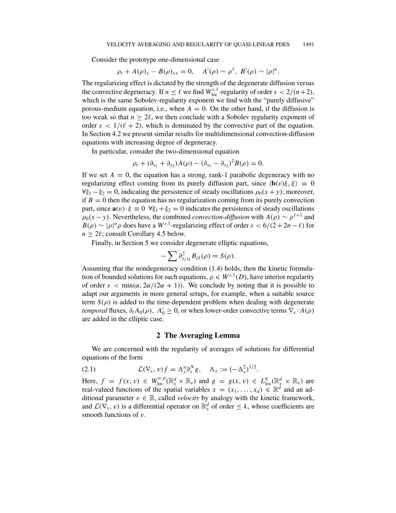
Consider the prototype one-dimensional case
ρt + A(ρ)x − B(ρ)xx = 0, A′(ρ) ∼ ρ�, B ′(ρ) ∼ |ρ|n.The regularizing effect is dictated by the strength of the degenerate diffusion versus
the convective degeneracy. If n ≤ � we find W s,1loc -regularity of order s < 2/(n+2),
which is the same Sobolev-regularity exponent we find with the “purely diffusive”
porous-medium equation, i.e., when A = 0. On the other hand, if the diffusion is
too weak so that n ≥ 2�, we then conclude with a Sobolev regularity exponent of
order s < 1/(� + 2), which is dominated by the convective part of the equation.
In Section 4.2 we present similar results for multidimensional convection-diffusion
equations with increasing degree of degeneracy.
In particular, consider the two-dimensional equation
ρt + (∂x1+ ∂x2
)A(ρ) − (∂x1− ∂x2
)2 B(ρ) = 0.
If we set A = 0, the equation has a strong, rank-1 parabolic degeneracy with no
regularizing effect coming from its purely diffusion part, since 〈b(v)ξ, ξ〉 ≡ 0
∀ξ1 − ξ2 = 0, indicating the persistence of steady oscillations ρ0(x + y); moreover,
if B = 0 then the equation has no regularization coming from its purely convection
part, since a(v) ·ξ ≡ 0 ∀ξ1 +ξ2 = 0 indicates the persistence of steady oscillations
ρ0(x − y). Nevertheless, the combined convection-diffusion with A(ρ) ∼ ρ�+1 and
B(ρ) ∼ |ρ|nρ does have a W s,1-regularizing effect of order s < 6/(2+2n − �) for
n ≥ 2�; consult Corollary 4.5 below.
Finally, in Section 5 we consider degenerate elliptic equations,
−∑
∂2xj xk
Bjk(ρ) = S(ρ).
Assuming that the nondegeneracy condition (1.4) holds, then the kinetic formula-
tion of bounded solutions for such equations, ρ ∈ W s,1(D), have interior regularity
of order s < min(α, 2α/(2α + 1)). We conclude by noting that it is possible to
adapt our arguments in more general setups, for example, when a suitable source
term S(ρ) is added to the time-dependent problem when dealing with degenerate
temporal fluxes, ∂t A0(ρ), A′0 ≥ 0, or when lower-order convective terms ∇x · A(ρ)
are added in the elliptic case.
2 The Averaging Lemma
We are concerned with the regularity of averages of solutions for differential
equations of the form
(2.1) L(∇x , v) f = ηx∂
Nv g, x := (−�2
x)1/2.
Here, f = f (x, v) ∈ W σ,ploc (Rd
x × Rv) and g = g(x, v) ∈ Lqloc(R
dx × Rv) are
real-valued functions of the spatial variables x = (x1, . . . , xd) ∈ Rd and an ad-
ditional parameter v ∈ R, called velocity by analogy with the kinetic framework,
and L(∇x , v) is a differential operator on Rdx of order ≤ k, whose coefficients are
smooth functions of v.
1492 E. TADMOR AND T. TAO
The velocity-averaging lemma asserts that if L( · , v) is nondegenerate in the
sense that its null set is sufficiently small (to be made precise below), then the
v-moments of f (x, · ),
f (x) :=∫v
f (x, v)φ(v)dv, φ ∈ C∞0 ,
are smoother than the usual regularity associated with the data of f (x, · ) and
g(x, · ). That is, by averaging over the so-called microscopic v-variable, there is a
gain of regularity in the macroscopic x-variables.
There is a relatively short yet intense history of such results, motivated by ki-
netic models such as Boltzmann, Vlasov, radiative transfer, and similar equations
where the v-moments of f represent macroscopic quantities of interest. We re-
fer to the early works of Agoshkov [1] and Golse, Lions, Perthame, and Sentis
[24, 25] treating first-order transport operators with f and g integrability of order
p = q > 1. The work of DiPerna, Lions, and Meyer [20] provided the first treat-
ment of the general case p �= q, followed by Bézard [4], the improved regularity
in [34], and an optimal Besov regularity result of DeVore and Petrova [16].
Extensions to more general streaming operators were treated by DiPerna and
Lions in [18, 19] with applications to Boltzmann and Vlasov-Maxwell equations,
and by Lions, Perthame, and Tadmor in [36] with applications to nonlinear con-
servation laws and related parabolic equations. Gérard [22] together with Golse
[23] provided an L2-treatment of general differential operators. A different line
of extensions consists of velocity-averaging lemmas that take into account dif-
ferent orders of integrability in x and v, leading to sharper velocity regulariza-
tion results sought in various applications. We refer to the results in [20] for
f ∈ L p1(Rv, L p2(Rdx )), g ∈ Lq1(Rv, Lq2(Rd
x )) and to Jabin and Vega [30] for f ∈W N1,p1(Rv, L p2(Rd
x )), g ∈ W N2,q1(Rv, Lq2(Rdx )). Westdickenberg [54] analyzed a
general case of the form f ∈ Bσp1,p2
(Rdx , Lr1(Rv)), g ∈ Bσ
q1,q2(Rd
x , Lr2(Rv)). Jabin,
Perthame, and Vega [29, 31] used a mixed integrability of
f ∈ L p(Rdx , W N1,p(Rv)), g ∈ Lq(Rd
x , W N2,q(Rv)),
to improve the regularizing results for nonlinear conservation laws [36, 37, 35],
Ginzburg-Landau, and other nonlinear models. Golse and Saint-Raymond [26]
showed that a minimal requirement of equi-integrability, say f ∈ L1(Rdx , L�(Rv))
and g ∈ L1(Rdx ×Rv) measured in Orlicz space L� with superlinear �, is sufficient
for relative compactness of the averages f , which otherwise might fail for mere
L1-integrability [24].
The derivation of velocity averaging in the above works was accomplished by
various methods. The main approach, which we use below, is based on decom-
position in Fourier space, carefully tracking f (ξ, v) in the “elliptic” region where
{v : L(iξ, v) �= 0} and the complement region, which is made sufficiently small
by a nondegeneracy assumption. Other approaches include the use of microlocal
VELOCITY AVERAGING AND REGULARITY OF QUASI-LINEAR PDES 1493
defect measures and H -measures [22, 48], wavelet decomposition [16], and “real-
space methods”—in time [5, 52] and in space-time using Radon transform [12, 54],
X-transform [30, 31], and duality-based dispersion estimates [26]. Almost all of
these results are devoted to the phenomena of velocity averaging in the context of
transport equations, k = 1.
Our study of velocity averaging applies to a large class of L’s satisfying the
so-called truncation property: in Section 2.4 we show that all L’s of order k ≤ 2
satisfy this truncation property. In particular, we improve the regularity statement
for first-order velocity averaging and extend the various velocity-averaging results
of the above works from first-order transport to general second-order transport-
diffusion and elliptic equations. The results are summarized in Averaging Lem-
mas 2.1 and 2.2 for homogeneous symbols and in Averaging Lemma 2.3 for gen-
eral, truncation-property-satisfying L’s. Our derivation is carried out in Fourier
space using Littlewood-Paley decompositions of f ∈ W σ,ploc (Rd
x × Rv) and g ∈Lq
loc(Rdx × Rv). To avoid an overload of indices, we leave for future work possible
extensions for more general data with mixed (x, v)–integrability of f and g.
2.1 The Truncation Property
We now come to a fundamental definition.
DEFINITION 2.1 Let m(ξ) be a complex-valued Fourier multiplier. We say that mhas the truncation property if, for any locally supported bump function ψ on C and
any 1 < p < ∞, the multiplier with symbol ψ(m(ξ)/δ) is an L p-multiplier uni-
formly in δ > 0, that is, its L p-multiplier norm depends solely on the support and
C� size of ψ (for some large � that may depend on m) but otherwise is independent
of δ.
In Section 2.4 we will describe some examples of multipliers with this trunca-
tion property. Equipped with this notion of a truncation property, we turn to discuss
the L p-size of parametrized multipliers. Let
Mψ f (x, v) := F−1x ψ
(m(ξ, v)
δ
)f (ξ, v)
denote the operator associated with the complex-valued multiplier m( · , v), trun-
cated at level δ, where f (ξ, v) = Fx f (ξ, v) := ∫Rd e−2π iξ ·x f (x, v)dx is the
Fourier transform of f ( · , v). Our derivation of the averaging lemmas below is
based on the following straightforward estimate for such parameterized multipli-
ers.
LEMMA 2.2 (Basic L p-Estimate) Let I be a finite interval, I ⊂ Rv, and assumem(ξ, v) satisfies the truncation property uniformly in v ∈ I . Let 1 < p ≤ 2. LetMψ denote the velocity-averaged Fourier multiplier
Mψ f (x) :=∫I
Mψ f (x, v)dv =∫I
F−1x ψ
(m(ξ, v)
δ
)Fx f (x, v)dv.
1494 E. TADMOR AND T. TAO
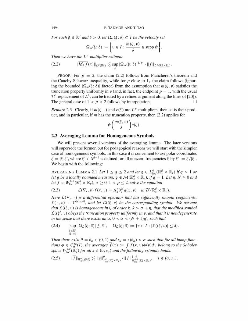
For each ξ ∈ Rd and δ > 0, let �m(ξ ; δ) ⊂ I be the velocity set
�m(ξ ; δ) :={v ∈ I : m(ξ, v)
δ∈ supp ψ
}.
Then we have the L p-multiplier estimate
(2.2) ‖Mψ f (x)‖L p(Rdx ) � sup
ξ
|�m(ξ ; δ)|1/p′ · ‖ f ‖L p(Rdx ×Rv).
PROOF: For p = 2, the claim (2.2) follows from Plancherel’s theorem and
the Cauchy-Schwarz inequality, while for p close to 1+ the claim follows (ignor-
ing the bounded |�m(ξ ; δ)| factor) from the assumption that m(ξ, v) satisfies the
truncation property uniformly in v (and, in fact, the endpoint p = 1, with the usual
H1 replacement of L1, can be treated by a refined argument along the lines of [20]).
The general case of 1 < p < 2 follows by interpolation. �
Remark 2.3. Clearly, if m(ξ, · ) and c(ξ) are L p-multipliers, then so is their prod-
uct, and in particular, if m has the truncation property, then (2.2) applies for
ψ
(m(ξ, v)
δ
)c(ξ).
2.2 Averaging Lemma for Homogeneous Symbols
We will present several versions of the averaging lemma. The later versions
will supersede the former, but for pedagogical reasons we will start with the simpler
case of homogeneous symbols. In this case it is convenient to use polar coordinates
ξ = |ξ |ξ ′, where ξ ′ ∈ Sd−1 is defined for all nonzero frequencies ξ by ξ ′ := ξ/|ξ |.We begin with the following:
AVERAGING LEMMA 2.1 Let 1 ≤ q ≤ 2 and let g ∈ Lqloc(R
dx × Rv) if q > 1 or
let g be a locally bounded measure, g ∈ M(Rdx × Rv), if q = 1. Let η, N ≥ 0 and
let f ∈ W σ,ploc (Rd
x × Rv), σ ≥ 0, 1 < p ≤ 2, solve the equation
(2.3) L(∇x , v) f (x, v) = ηx∂
Nv g(x, v) in D
′(Rdx × Rv).
Here L(∇x , · ) is a differential operator that has sufficiently smooth coefficients,L( · , v) ∈ C N ,ε>0, and let L(iξ, v) be the corresponding symbol. We assumethat L(iξ, v) is homogeneous in ξ of order k, k > σ + η, that the modified symbolL(iξ ′, v) obeys the truncation property uniformly in v, and that it is nondegeneratein the sense that there exists an α, 0 < α < (N + 1)q ′, such that
(2.4) supξ∈R
d
|ξ |=1
|�L(ξ ; δ)| � δα, �L(ξ ; δ) := {v ∈ I : |L(iξ, v)| ≤ δ}.
Then there exist θ = θα ∈ (0, 1) and sα = s(θα) > σ such that for all bump func-tions φ ∈ C∞
0 (I ), the averages f (x) := ∫f (x, v)φ(v)dv belong to the Sobolev
space W s,rloc (Rd
x ) for all s ∈ (σ, sα) and the following estimate holds:
(2.5) ‖ f ‖W s,rloc (Rd
x ) � ‖g‖θ
Lqloc(R
dx ×Rv)
· ‖ f ‖1−θ
W σ,ploc (Rd
x ×Rv), s ∈ (σ, sα).
VELOCITY AVERAGING AND REGULARITY OF QUASI-LINEAR PDES 1495
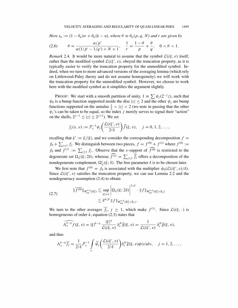
Here sα := (1 − θα)σ + θα(k − η), where θ ≡ θα(p, q, N ) and r are given by
(2.6) θ = α/p′
α(1/p′ − 1/q ′) + N + 1,
1
r= 1 − θ
p+ θ
q, 0 < θ < 1.
Remark 2.4. It would be more natural to assume that the symbol L(iξ, v) itself,
rather than the modified symbol L(iξ ′, v), obeyed the truncation property, as it is
typically easier to verify the truncation property for the unmodified symbol. In-
deed, when we turn to more advanced versions of the averaging lemma (which rely
on Littlewood-Paley theory and do not assume homogeneity) we will work with
the truncation property for the unmodified symbol. However, we choose to work
here with the modified symbol as it simplifies the argument slightly.
PROOF: We start with a smooth partition of unity, 1 ≡ ∑ψj (2
− j z), such that
ψ0 is a bump function supported inside the disc |z| ≤ 2 and the other ψj are bump
functions supported on the annulus 12
< |z| < 2 (we note in passing that the other
ψj ’s can be taken to be equal, so the index j merely serves to signal their “action”
on the shells, 2 j−1 ≤ |z| ≤ 2 j+1). We set
f j (x, v) := F−1x ψj
(L(iξ ′, v)
2 jδ
)f (ξ, v), j = 0, 1, 2, . . . ,
recalling that ξ ′ := ξ/|ξ |, and we consider the corresponding decomposition f =f0 + ∑
j≥1 f j . We distinguish between two pieces, f = f (0) + f (1) where f (0) :=f0 and f (1) := ∑
j≥1 f j . Observe that the v-support of f (0) is restricted to the
degenerate set �L(ξ ; 2δ), whereas f (1) = ∑j≥1 f j offers a decomposition of the
nondegenerate complement, �cL(ξ ; δ). The free parameter δ is to be chosen later.
We first note that f (0) = f0 is associated with the multiplier ψ0(L(iξ ′, v)/δ).
Since L(iξ ′, v) satisfies the truncation property, we can use Lemma 2.2 and the
nondegeneracy assumption (2.4) to obtain
‖ f (0)‖W σ,ploc (Rd
x ) � sup|ξ |=1
∣∣∣∣�L(ξ ; 2δ)
∣∣∣∣1/p′
· ‖ f ‖W σ,ploc (Rd
x ×Rv)
� δα/p′‖ f ‖W σ,ploc (Rd
x ×Rv).
(2.7)
We turn to the other averages f j , j ≥ 1, which make f (1). Since L(iξ, · ) is
homogeneous of order k, equation (2.3) states that
k−ηx f (ξ, v) = |ξ |k−η |ξ |η
L(iξ, v)∂ Nv g(ξ, v) = 1
L(iξ ′, v)∂ Nv g(ξ, v),
and thus
k−ηx f j = 1
2 jδF
−1x
∫v
ψj
(L(iξ ′, v)
2 jδ
)∂ Nv g(ξ, v)φ(v)dv, j = 1, 2, . . . ,
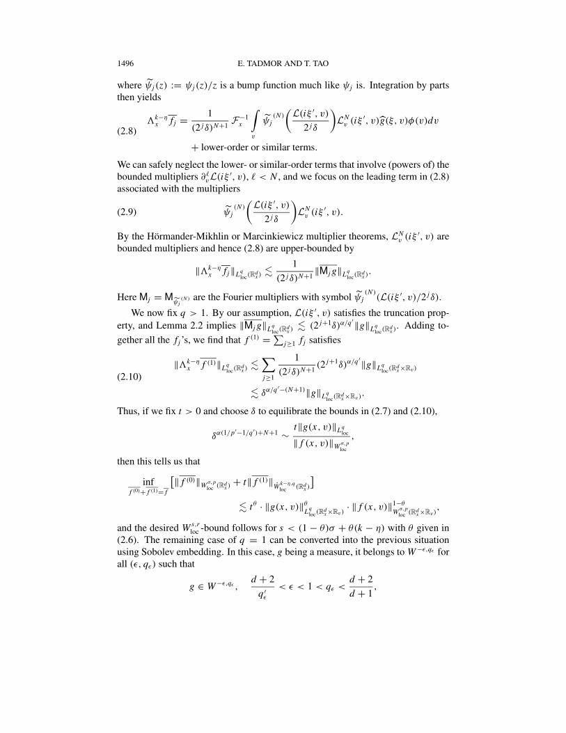
1496 E. TADMOR AND T. TAO
where ψj (z) := ψj (z)/z is a bump function much like ψj is. Integration by parts
then yields
k−ηx f j = 1
(2 jδ)N+1F
−1x
∫v
ψj(N )
(L(iξ ′, v)
2 jδ
)L
Nv (iξ ′, v)g(ξ, v)φ(v)dv
+ lower-order or similar terms.
(2.8)
We can safely neglect the lower- or similar-order terms that involve (powers of) the
bounded multipliers ∂�vL(iξ ′, v), � < N , and we focus on the leading term in (2.8)
associated with the multipliers
(2.9) ψj(N )
(L(iξ ′, v)
2 jδ
)L
Nv (iξ ′, v).
By the Hörmander-Mikhlin or Marcinkiewicz multiplier theorems, LNv (iξ ′, v) are
bounded multipliers and hence (2.8) are upper-bounded by
‖ k−ηx f j‖Lq
loc(Rdx ) �
1
(2 jδ)N+1‖Mj g‖Lq
loc(Rdx ).
Here Mj = Mψj
(N ) are the Fourier multipliers with symbol ψj(N )
(L(iξ ′, v)/2 jδ).
We now fix q > 1. By our assumption, L(iξ ′, v) satisfies the truncation prop-
erty, and Lemma 2.2 implies ‖Mj g‖Lqloc(R
dx ) � (2 j+1δ)α/q ′‖g‖Lq
loc(Rdx ). Adding to-
gether all the f j ’s, we find that f (1) = ∑j≥1 f j satisfies
‖ k−ηx f (1)‖Lq
loc(Rdx ) �
∑j≥1
1
(2 jδ)N+1(2 j+1δ)α/q ′‖g‖Lq
loc(Rdx ×Rv)
� δα/q ′−(N+1)‖g‖Lqloc(R
dx ×Rv)
.
(2.10)
Thus, if we fix t > 0 and choose δ to equilibrate the bounds in (2.7) and (2.10),
δα(1/p′−1/q ′)+N+1 ∼t‖g(x, v)‖Lq
loc
‖ f (x, v)‖W σ,ploc
,
then this tells us that
inff (0)+ f (1)= f
[‖ f (0)‖W σ,ploc (Rd
x ) + t‖ f (1)‖W k−η,qloc (Rd
x )
]� tθ · ‖g(x, v)‖θ
Lqloc(R
dx ×Rv)
· ‖ f (x, v)‖1−θ
W σ,ploc (Rd
x ×Rv),
and the desired W s,rloc -bound follows for s < (1 − θ)σ + θ(k − η) with θ given in
(2.6). The remaining case of q = 1 can be converted into the previous situation
using Sobolev embedding. In this case, g being a measure, it belongs to W −ε,qε for
all (ε, qε) such that
g ∈ W −ε,qε ,d + 2
q ′ε
< ε < 1 < qε <d + 2
d + 1,
VELOCITY AVERAGING AND REGULARITY OF QUASI-LINEAR PDES 1497
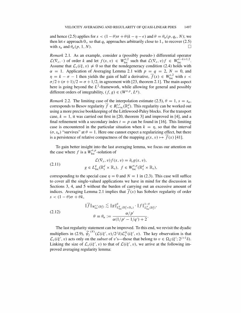
and hence (2.5) applies for s < (1 − θ)σ + θ(k − η − ε) and θ = θα(p, qε, N ); we
then let ε approach 0+ so that qε approaches arbitrarily close to 1+ to recover (2.5)
with sα and θα(p, 1, N ). �
Remark 2.1. As an example, consider a (possibly pseudo-) differential operator
L(∇x , · ) of order k and let f (x, v) ∈ W σ,2loc such that L(∇x , v) f ∈ W σ−k+1,2
loc .
Assume that Lv(iξ, v) �= 0 so that the nondegeneracy condition (2.4) holds with
α = 1. Application of Averaging Lemma 2.1 with p = q = 2, N = 0, and
η = k − σ − 1 then yields the gain of half a derivative, f (x) ∈ W s,2loc with s <
σ/2+ (σ +1)/2 = σ +1/2, in agreement with [23, theorem 2.1]. The main aspect
here is going beyond the L2-framework, while allowing for general and possibly
different orders of integrability, ( f, g) ∈ (W σ,p, Lq).
Remark 2.2. The limiting case of the interpolation estimate (2.5), θ = 1, s = sα,
corresponds to Besov regularity f ∈ Bs,rt=∞(Rd
x ). This regularity can be worked out
using a more precise bookkeeping of the Littlewood-Paley blocks. For the transport
case, k = 1, it was carried out first in [20, theorem 3] and improved in [4], and a
final refinement with a secondary index t = p can be found in [16]. This limiting
case is encountered in the particular situation when k = η, so that the interval
(σ, sα) “survives” at θ = 1. Here one cannot expect a regularizing effect, but there
is a persistence of relative compactness of the mapping g(x, v) �→ f (x) [41].
To gain better insight into the last averaging lemma, we focus our attention on
the case where f is a W σ,ploc -solution of
(2.11)L(∇x , v) f (x, v) = ∂vg(x, v),
g ∈ Lqloc(R
dx × Rv), f ∈ W σ,p
loc (Rdx × Rv),
corresponding to the special case η = 0 and N = 1 in (2.3). This case will suffice
to cover all the single-valued applications we have in mind for the discussion in
Sections 3, 4, and 5 without the burden of carrying out an excessive amount of
indices. Averaging Lemma 2.1 implies that f (x) has Sobolev regularity of order
s < (1 − θ)σ + θk,
(2.12)
‖ f ‖W s,rloc (Rd
x ) � ‖g‖θ
Lqloc(R
dx ×Rv)
· ‖ f ‖1−θ
L ploc(R
dx ),
θ ≡ θα := α/p′
α(1/p′ − 1/q ′) + 2.
The last regularity statement can be improved. To this end, we revisit the dyadic
multipliers in (2.9), ψj(N )
(L(iξ ′, v)/2 jδ)LNv (iξ ′, v). The key observation is that
Lv(iξ ′, v) acts only on the subset of v’s—those that belong to v ∈ �L(ξ ′; 2 j+1δ).
Linking the size of Lv(iξ ′, v) to that of L(iξ ′, v), we arrive at the following im-
proved averaging regularity lemma:
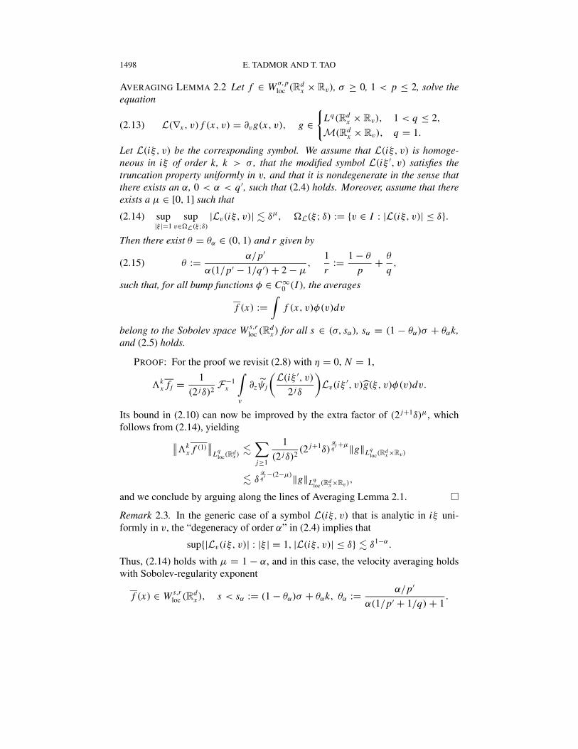
1498 E. TADMOR AND T. TAO
AVERAGING LEMMA 2.2 Let f ∈ W σ,ploc (Rd
x × Rv), σ ≥ 0, 1 < p ≤ 2, solve theequation
(2.13) L(∇x , v) f (x, v) = ∂vg(x, v), g ∈{
Lq(Rdx × Rv), 1 < q ≤ 2,
M(Rdx × Rv), q = 1.
Let L(iξ, v) be the corresponding symbol. We assume that L(iξ, v) is homoge-neous in iξ of order k, k > σ , that the modified symbol L(iξ ′, v) satisfies thetruncation property uniformly in v, and that it is nondegenerate in the sense thatthere exists an α, 0 < α < q ′, such that (2.4) holds. Moreover, assume that thereexists a µ ∈ [0, 1] such that
(2.14) sup|ξ |=1
supv∈�L(ξ ;δ)
|Lv(iξ, v)| � δµ, �L(ξ ; δ) := {v ∈ I : |L(iξ, v)| ≤ δ}.
Then there exist θ = θα ∈ (0, 1) and r given by
(2.15) θ := α/p′
α(1/p′ − 1/q ′) + 2 − µ,
1
r:= 1 − θ
p+ θ
q,
such that, for all bump functions φ ∈ C∞0 (I ), the averages
f (x) :=∫
f (x, v)φ(v)dv
belong to the Sobolev space W s,rloc (Rd
x ) for all s ∈ (σ, sα), sα = (1 − θα)σ + θαk,and (2.5) holds.
PROOF: For the proof we revisit (2.8) with η = 0, N = 1,
kx f j = 1
(2 jδ)2F
−1x
∫v
∂zψj
(L(iξ ′, v)
2 jδ
)Lv(iξ
′, v)g(ξ, v)φ(v)dv.
Its bound in (2.10) can now be improved by the extra factor of (2 j+1δ)µ, which
follows from (2.14), yielding∥∥ kx f (1)
∥∥Lq
loc(Rdx )
�∑j≥1
1
(2 jδ)2(2 j+1δ)
αq′ +µ‖g‖Lq
loc(Rdx ×Rv)
� δαq′ −(2−µ)‖g‖Lq
loc(Rdx ×Rv)
,
and we conclude by arguing along the lines of Averaging Lemma 2.1. �
Remark 2.3. In the generic case of a symbol L(iξ, v) that is analytic in iξ uni-
formly in v, the “degeneracy of order α” in (2.4) implies that
sup{|Lv(iξ, v)| : |ξ | = 1, |L(iξ, v)| ≤ δ} � δ1−α.
Thus, (2.14) holds with µ = 1 − α, and in this case, the velocity averaging holds
with Sobolev-regularity exponent
f (x) ∈ W s,rloc (Rd
x ), s < sα := (1 − θα)σ + θαk, θα := α/p′
α(1/p′ + 1/q) + 1.
VELOCITY AVERAGING AND REGULARITY OF QUASI-LINEAR PDES 1499
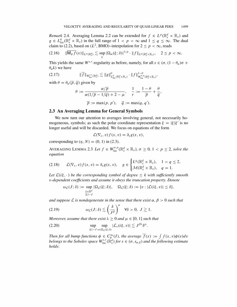
Remark 2.4. Averaging Lemma 2.2 can be extended for f ∈ L p(Rdx × Rv) and
g ∈ Lqloc(R
dx × Rv) in the full range of 1 < p < ∞ and 1 ≤ q ≤ ∞. The dual
claim to (2.2), based on (L2, BMO)–interpolation for 2 ≤ p < ∞, reads
(2.16) ‖Mψ f (x)‖L p(Rdx ) � sup
ξ
|�m(ξ ; δ)|1/p · ‖ f ‖L p(Rdx ×Rv), 2 ≤ p < ∞.
This yields the same W s,r -regularity as before, namely, for all s ∈ (σ, (1 − θα)σ +θαk) we have
(2.17) ‖ f ‖W s,rloc (Rd
x ) � ‖g‖θ
Lqloc(R
dx ×Rv)
· ‖ f ‖1−θ
W σ,ploc (Rd
x ×Rv),
with θ = θα(p, q) given by
θ := α/p
α(1/p − 1/q) + 2 − µ,
1
r:= 1 − θ
p+ θ
q,
p := max(p, p′), q := max(q, q ′).
2.3 An Averaging Lemma for General Symbols
We now turn our attention to averages involving general, not necessarily ho-
mogeneous, symbols; as such the polar coordinate representation ξ = |ξ |ξ ′ is no
longer useful and will be discarded. We focus on equations of the form
L(∇x , v) f (x, v) = ∂vg(x, v),
corresponding to (η, N ) = (0, 1) in (2.3).
AVERAGING LEMMA 2.3 Let f ∈ W σ,ploc (Rd
x × Rv), σ ≥ 0, 1 < p ≤ 2, solve theequation
(2.18) L(∇x , v) f (x, v) = ∂vg(x, v), g ∈{
Lq(Rdx × Rv), 1 < q ≤ 2,
M(Rdx × Rv), q = 1.
Let L(iξ, · ) be the corresponding symbol of degree ≤ k with sufficiently smoothv-dependent coefficients and assume it obeys the truncation property. Denote
ωL(J ; δ) := supξ∈R
d
|ξ |∼J
|�L(ξ ; δ)|, �L(ξ ; δ) := {v : |L(iξ, v)| ≤ δ},
and suppose L is nondegenerate in the sense that there exist α, β > 0 such that
(2.19) ωL(J ; δ) �
(δ
J β
)α
∀δ > 0, J � 1.
Moreover, assume that there exist λ ≥ 0 and µ ∈ [0, 1] such that
(2.20) sup|ξ |∼J
supv∈�L(ξ ;δ)
|Lv(iξ, v)| � J βλδµ.
Then for all bump functions φ ∈ C∞0 (I ), the average f (x) := ∫
f (x, v)φ(v)dv
belongs to the Sobolev space W s,rloc (Rd
x ) for s ∈ (σ, sα,β) and the following estimateholds:
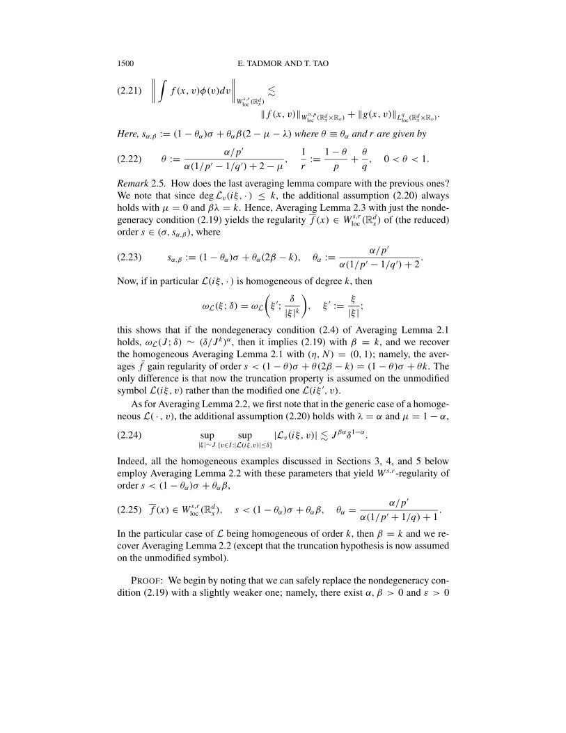
1500 E. TADMOR AND T. TAO
(2.21)
∥∥∥∥ ∫f (x, v)φ(v)dv
∥∥∥∥W s,r
loc (Rdx )
�
‖ f (x, v)‖W σ,ploc (Rd
x ×Rv)+ ‖g(x, v)‖Lq
loc(Rdx ×Rv)
.
Here, sα,β := (1 − θα)σ + θαβ(2 − µ − λ) where θ ≡ θα and r are given by
(2.22) θ := α/p′
α(1/p′ − 1/q ′) + 2 − µ,
1
r:= 1 − θ
p+ θ
q, 0 < θ < 1.
Remark 2.5. How does the last averaging lemma compare with the previous ones?
We note that since degLv(iξ, · ) ≤ k, the additional assumption (2.20) always
holds with µ = 0 and βλ = k. Hence, Averaging Lemma 2.3 with just the nonde-
generacy condition (2.19) yields the regularity f (x) ∈ W s,rloc (Rd
x ) of (the reduced)
order s ∈ (σ, sα,β), where
(2.23) sα,β := (1 − θα)σ + θα(2β − k), θα := α/p′
α(1/p′ − 1/q ′) + 2.
Now, if in particular L(iξ, · ) is homogeneous of degree k, then
ωL(ξ ; δ) = ωL
(ξ ′; δ
|ξ |k)
, ξ ′ := ξ
|ξ | ;
this shows that if the nondegeneracy condition (2.4) of Averaging Lemma 2.1
holds, ωL(J ; δ) ∼ (δ/J k)α, then it implies (2.19) with β = k, and we recover
the homogeneous Averaging Lemma 2.1 with (η, N ) = (0, 1); namely, the aver-
ages f gain regularity of order s < (1 − θ)σ + θ(2β − k) = (1 − θ)σ + θk. The
only difference is that now the truncation property is assumed on the unmodified
symbol L(iξ, v) rather than the modified one L(iξ ′, v).
As for Averaging Lemma 2.2, we first note that in the generic case of a homoge-
neous L( · , v), the additional assumption (2.20) holds with λ = α and µ = 1 − α,
(2.24) sup|ξ |∼J
sup{v∈I :|L(iξ,v)|≤δ}
|Lv(iξ, v)| � J βαδ1−α.
Indeed, all the homogeneous examples discussed in Sections 3, 4, and 5 below
employ Averaging Lemma 2.2 with these parameters that yield W s,r -regularity of
order s < (1 − θα)σ + θαβ,
(2.25) f (x) ∈ W s,rloc (Rd
x ), s < (1 − θα)σ + θαβ, θα = α/p′
α(1/p′ + 1/q) + 1.
In the particular case of L being homogeneous of order k, then β = k and we re-
cover Averaging Lemma 2.2 (except that the truncation hypothesis is now assumed
on the unmodified symbol).
PROOF: We begin by noting that we can safely replace the nondegeneracy con-
dition (2.19) with a slightly weaker one; namely, there exist α, β > 0 and ε > 0
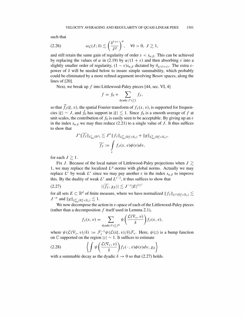
VELOCITY AVERAGING AND REGULARITY OF QUASI-LINEAR PDES 1501
such that
(2.26) ωL(J ; δ) �
(δ1+ε
J β
)α
, ∀δ > 0, J � 1,
and still retain the same gain of regularity of order s < sα,β . This can be achieved
by replacing the values of α in (2.19) by α/(1 + ε) and then absorbing ε into a
slightly smaller order of regularity, (1 − ε)sα,β dictated by θα/(1+ε). The extra ε-
power of δ will be needed below to insure simple summability, which probably
could be eliminated by a more refined argument involving Besov spaces, along the
lines of [20].
Next, we break up f into Littlewood-Paley pieces [44, sec. VI, 4]
f = f0 +∑
dyadic J ’s�1
f J ,
so that f J (ξ, v), the spatial Fourier transform of f J (x, v), is supported for frequen-
cies |ξ | ∼ J , and f0 has support in |ξ | � 1. Since f0 is a smooth average of f at
unit scales, the contribution of f0 is easily seen to be acceptable. By giving up an ε
in the index sα,β we may thus reduce (2.21) to a single value of J . It thus suffices
to show that
J s‖ f J ‖Lrloc(R
d ) � J σ‖ f J ‖L ploc(R
dx ×Rv)
+ ‖g‖Lqloc(R
dx ×Rv)
,
f J :=∫v
f J (x, v)φ(v)dv,
for each J � 1.
Fix J . Because of the local nature of Littlewood-Paley projections when J �1, we may replace the localized L p-norms with global norms. Actually we may
replace Lr by weak Lr since we may pay another ε in the index sα,β to improve
this. By the duality of weak Lr and Lr ′,1, it thus suffices to show that
(2.27) |〈 f J , χE〉| � J −s |E |1/r ′
for all sets E ⊂ Rd of finite measure, where we have normalized ‖ f J ‖L p(Rdx ×Rv) �
J −σ and ‖g‖Lqloc(R
dx ×Rv)
� 1.
We now decompose the action in v-space of each of the Littlewood-Paley pieces
(rather than a decomposition f itself used in Lemma 2.1),
f J (x, v) =∑
dyadic δ’s�J k
ψ
(L(∇x , v)
δ
)f J (x, v),
where ψ(L(∇x , v)/δ) := F−1x ψ(L(iξ, v)/δ)Fx . Here, ψ(z) is a bump function
on C supported on the region |z| ∼ 1. It suffices to estimate
(2.28)
⟨ ∫ψ
(L(∇x , v)
δ
)f J ( · , v)φ(v)dv, χE
⟩with a summable decay as the dyadic δ → 0 so that (2.27) holds.
1502 E. TADMOR AND T. TAO
By our assumption, L(iξ, v) satisfies the truncation property uniformly in v;
hence by Lemma 2.2 we see that for all 1 < p ≤ 2,
(2.29)
∥∥∥∥ ∫ψ
(L(∇x , v)
δ
)f J (x, v)φ(v)dv
∥∥∥∥L p
loc(Rdx )
�
ωL(J ; δ)1/p′‖ f J ‖L ploc(R
dx ×Rv)
.
From (2.29) and Hölder we may thus estimate (2.28) by
(2.30)
∣∣∣∣⟨ ∫ψ
(L(∇x , v)
δ
)f J ( · , v)φ(v)dv, χE
⟩∣∣∣∣ � J −σωL(J ; δ)1/p′ |E |1/p′.
On the other hand, thanks to equation (2.18) we can write
ψ
(L(∇x , v)
δ
)f J (x, v) = ψ
(L(∇x , v)
δ
)1
δ
∂
∂vgJ (x, v)
where ψ(z) := ψ(z)/z and the gJ ’s are the corresponding Littlewood-Paley dyadic
pieces of g. We thus have
(2.31)
∫ψ
(L(∇x , v)
δ
)f J (x, v)φ(v)dv =
1
δ
∫ψ
(L(∇x , v)
δ
)∂
∂vgJ (x, v)φ(v)dv.
We now integrate by parts to move the ∂/∂v derivative somewhere else. We will
assume that the derivative hits ψ(L(∇x , v)/δ), since the case when the derivative
hits the bump function φ(v) is much better. We are thus led to estimate
(2.32)1
δ2
∣∣∣∣⟨ ∫ψz
(L(∇x , v)
δ
)Lv(∇x , v)gJ (x, v)φ(v)dv, χE
⟩∣∣∣∣.Since gJ is localized to frequencies ∼ J , then by (2.20), the multiplier Lv(iξ, v)
acts like a constant of order O(J βλδµ). Also, ψz is a bump function much like ψ .
Thus we may modify (2.29) with p replaced by q (assuming that q > 1 and using
the modified argument for the case q = 1 as before), ψ replaced by ψz , and f J
replaced by Lv(∇x , v)gJ , to estimate (2.31) by
(2.33)
∣∣∣∣⟨ ∫ψ
(L(∇x , v)
δ
)f J ( · , v)φ(v)dv, χE
⟩∣∣∣∣ �
δ−(2−µ) J βλωL(J ; δ)1/q ′ |E |1/q ′.
Interpolating this bound with (2.30), we may bound (2.28) by
δ−θ(2−µ) J (1−θ)(−σ)+θβλωL(J ; δ)1/r ′ |E |1/r ′.
The parametrization in (2.22) dictates α/r ′ = θ(2 − µ). Finally, we put the extra
ε power into use: by (2.26), ωL(J ; δ)1/r ′� (δ1+ε J −β)θ(2−µ) and hence the last
VELOCITY AVERAGING AND REGULARITY OF QUASI-LINEAR PDES 1503
quantity is bounded by
δθ(2−µ)ε J −sα,β |E |1/r ′, sα,β = (1 − θ)σ − θβ(2 − µ − λ).
Summing in δ and using the hypothesis that s < sα,β , we obtain (2.27). �
2.4 Velocity Averaging for First- and Second-Order Symbols
To apply velocity Averaging Lemma 2.3 we need to find out which multipliers
m(ξ) have the truncation property. Fortunately, there are large classes of such
multipliers.
First of all, it is clear that the multipliers m(ξ) = ξ ·e1 and m(ξ) = |ξ |2 have the
truncation property, as in these cases the Fourier multipliers are just convolutions
with finite measures. Now, observe that if m(ξ) has the truncation property, then so
does m(L(ξ)) for any invertible linear transformation L on Rd , with a bound that
is uniform in L . This is because the L p-multiplier class is invariant under linear
transformations.
Because of this, we see that the multipliers
m1(ξ) = a(v) · iξ and m2(ξ) = 〈b(v)ξ, ξ〉have the truncation property uniformly in v, where a(v) are arbitrary real coeffi-
cients and b(v) is an arbitrary elliptic bilinear form with real coefficients.
From the Hörmander-Mikhlin or Marcinkeiwicz multiplier theorems and the
linear transformation argument one can also show that m1(ξ′) has the truncation
property uniformly in v. These arguments go back to the discussion of [20]. The
situation with m2(ξ′) is less clear, but fortunately we will not need to verify that
these second-order modified multipliers obey the truncation property since our av-
eraging lemmas also work with a truncation property hypothesis on the unmodified
multiplier.
Now we observe that if m1(ξ) and m2(ξ) are real multipliers with the truncation
property, then the complex multiplier m1(ξ)+ im2(ξ) also has the truncation prop-
erty. The basic observation is that one can use Fourier series to write any symbol
of the form
ψ
(m1(ξ) + im2(ξ)
δ
)as ∑
j,k∈Z
ψ( j, k)ψj
(m1(ξ)
δ
)ψk
(m2(ξ)
δ
)where ψj (x) := e2π i j x ψ and ψ is some bump function that equals 1 on the one-
dimensional projections of the support of ψ . Since the C�-norm of ψj grows poly-
nomially in j and ψ( j, k) decays rapidly in j and k (if ψ is sufficiently smooth),
we are done since the product of two L p-multipliers is still an L p-multiplier.
1504 E. TADMOR AND T. TAO
3 Nonlinear Hyperbolic Conservation Laws
Having developed our averaging lemmas, we now present some applications
to nonlinear PDEs. We begin with the study of (real-valued) solutions ρ(t, x) =ρ(t, x1, . . . , xd) ∈ L∞((0,∞)×Rd
x ) of multidimensional scalar conservation laws,
(3.1)∂
∂tρ(t, x) +
d∑j=1
∂
∂xjAj (ρ(t, x)) = 0 in D
′((0,∞) × Rdx ).
We abbreviate (3.1) as ρt + ∇x · A(ρ) = 0 where A is the vector of C2,ε-spatial
fluxes, A := (A1, A2, . . . , Ad). Let χγ (v) denote the velocity indicator function
χγ (v) =
1 if 0 < v ≤ γ
−1 if γ ≤ v < 0
0 otherwise.
We say that ρ(t, x) is a kinetic solution of the conservation law (3.1) if the corre-
sponding distribution function χρ(t,x)(v) satisfies the transport equation
(3.2) ∂tχρ(t,x)(v)+a(v) ·∇xχρ(t,x)(v) = ∂vm(t, x, v) in D′((0,∞)×Rd
x ×Rv),
for some nonnegative measure, m(t, x, v) ∈ M+((0,∞) × Rdx × Rv). Here, a(v)
is the vector of transport velocities, a(v) := (a1(v), . . . , ad(v)) where aj (·) :=A′
j (·), j = 1, . . . , d. The regularizing effect associated with the proper notion of
nonlinearity of the conservation law (3.1) was explored in [36] through the averag-
ing properties of an underlying kinetic formulation. For completeness, we include
here a brief description that will serve our discussion on nonlinear parabolic and
elliptic equations in the following sections, and we refer to [36] for a complete
discussion.
The starting point is the entropy inequalities associated with (3.1),
∂tη(ρ(t, x)) + ∇x · Aη(ρ(t, x)) ≤ 0 in D′((0,∞) × Rd
x ).
Here, η is an arbitrary entropy function (a convex function from R to R) and
Aη := (Aη
1, . . . , Aη
d) is the corresponding vector of entropy fluxes, Aη
j (ρ) :=∫ ρη′(s)A′
j (s)ds, j = 1, . . . , d. A function ρ ∈ L∞ is an entropy solution if
it satisfies the entropy inequalities for all pairs (η, Aη) induced by convex en-
tropies η. Entropy solutions are precisely those solutions that are realizable as
vanishing viscosity limit solutions and are uniquely determined by their L∞ ∩ L1–
initial data ρ0(x), prescribed at t = 0, e.g., [33]. A decisive role is played by the
one-parameter family of Kružkov entropy pairs, (η(ρ; v), Aη(ρ; v)), parametrized
by v ∈ R,
η(ρ; v) := |ρ − v|, Aη
j (ρ; v) := sgn(ρ − v)(Aj (ρ) − Aj (v)).
Kružkov entropy pairs lead to a complete L1-theory of existence, uniqueness, and
stability of first-order quasi-linear conservation laws [32].
VELOCITY AVERAGING AND REGULARITY OF QUASI-LINEAR PDES 1505
We turn to the kinetic formulation. We define the distribution m(t, x, v) =mρ(t,x)(v) by the formula
(3.3) m(t, x, v) := −[∂t
η(ρ; v) − η(0; v)
2+ ∇x ·
(Aη(ρ; v) − Aη(0; v)
2
)].
The entropy inequalities tell us that the distribution m = mρ is in fact a nonnegative
measure, m(t, x, v) ∈ M+((0,∞)×Rdx ×Rv). Next, we differentiate (3.3) with re-
spect to v: a straightforward computation yields that χρ(t,x)(v) satisfies the kinetic
transport equation (3.2). This reveals the interplay between Kružkov entropy in-
equalities and the underlying kinetic formulation; for nonlinear conservation laws,
kinetic solutions coincide with the entropy solutions [36, 40, 43]. Observe that
by velocity averaging we recover the macroscopic quantities associated with the
entropy solution ρ, ∫v
χρ(v)φ(v)dv = �(ρ),
where �(ρ) := ∫ ρ
s=0φ(s)ds is the primitive of φ. In particular, one can recover ρ
itself by setting φ(v) = 1[−M,M](v), M = ‖ρ‖L∞ .
We now use Averaging Lemma 2.2 to study the regularity of ρ. To this end
we first extend (3.2) over the full Rt × Rdx –space, using a C∞
0 (0,∞)–cutoff func-
tion, ψ ≡ 1 for t ≥ ε, so that f (t, x, v) := χρ(t,x)(v)ψ(t) and g(t, x, v) :=mv(t, x, v)ψ(t) + χρ(t,x)(v)∂tψ(t) satisfy
∂t f (t, x, v) + a(v) · ∇x f (t, x, v) = ∂vg(t, x, v) in D′(Rt × Rd
x × Rv),
with g ∈ M(Rt ×Rdx ×Rv). Set I := [inf ρ0, sup ρ0] and assume that the first-order
symbol is nondegenerate so that (2.4), (2.14) hold; namely, there exist α ∈ (0, 1)
and µ ∈ [0, 1] such that
(3.4) supτ 2+|ξ |2=1
|�a(ξ ; δ)| � δα, �a(ξ ; δ) := {v ∈ I : |τ + a(v) · ξ | ≤ δ},
and
(3.5) sup|ξ |=1
sup�a(ξ ;δ)
|a′(v) · ξ | � δµ.
We apply Averaging Lemma 2.2 for first-order symbols, k = 1, with q = 1,
p = 2, and σ = 0, to find that f (x) and hence ρ(x) belongs to W s,rloc (Rt × Rd
x ),
ρ(t, x) ∈ W s,rloc ((ε,∞) × Rd
x ), s < θα := α
α + 4 − 2µ, r := α + 4 − 2µ
α + 2 − µ.
At this stage we invoke the monotonicity property of entropy solutions, which
implies that for s < 1, ‖ρ(t, · )‖W s,1loc (Rd
x )is nonincreasing, and we deduce that
ρ(t, · ) ∈ W s,1(Rdx ) for t > ε. We conclude that the entropy solution operator
1506 E. TADMOR AND T. TAO
associated with the nonlinear conservation law (3.1),(3.4), ρ0(·) �→ ρ(t, · ), has a
regularizing effect, mapping L∞(Rdx ) into W s,1
loc (Rdx ),
∀t ≥ ε > 0 ρ(t, · ) ∈ W s,1loc (Rd
x ), s < s1, s1 := θα = α
α + 4 − 2µ.
Next, we use the bootstrap argument of [36, sec. 3] to deduce an improved
regularizing effect. The W s,1loc (Rt × Rd
x )–regularity of ρ(t, x)ψ(t) implies that
f (t, x, v) = χρ(t,x)(v)ψ(t) belongs to L1(W s,1(Rt × Rdx ), Rv); moreover, since
∂vχρ(v) is a bounded measure, f ∈ L1(W s,1(Rt ×Rdx ), Rv)∩L1(Rt ×Rd
x , W s,1(Rv))
and hence
f ∈ W s,1loc (Rt × Rd
x × Rv) ∀s < s1.
Interpolation with the obvious L∞-bound of f then yields that f ∈ W s,2loc (Rt ×
Rdx × Rv) for all s < s1/2. Therefore, Averaging Lemma 2.2 applies to f =
χρ(t,x)(v)ψ(t) with q = 1, p = 2, and σ = s1/2, implying that ρ(t, · ) has im-
proved W s,1loc -regularity of order s < s2 = (1 − θα)s1/2 + θα. Reiterating this
argument yields the fixed point sk ↑ s∞ = 2θα/(1 + θα) and we conclude with a
regularizing effect
∀t ≥ ε > 0 ρ0 ∈ L∞ ∩ L1(Rdx ) �→ ρ(t, · ) ∈ W s,1
loc (Rdx ), s <
α
α + 2 − µ.
As indicated earlier in Remark 2.5, in the generic case, µ = 1 − α,
(3.6) sup|ξ |=1
sup{v∈I :|τ+a(v)·ξ |≤δ}
|a′(v) · ξ | � δ1−α,
which yields a W s,1-regularizing effect of order s < α/(2α+1). This improves the
previous regularity result [36, theorem 4] of order s < α/(α + 2), corresponding
to µ = 0.
We can extend the last statement for general L ploc initial data. Recall that the
entropy solution operator associated with (3.1) is L1-contractive. We now in-
voke a general nonlinear interpolation argument of J.-L. Lions, e.g., [49, “Inter-
polation Theory,” lecture 8]; namely, if a possibly nonlinear T is Lipschitz on Xwith a Lipschitz constant L X and maps boundedly Y1 �→ Y2 with a bound BY ,
then one verifies that the corresponding K -functional satisfies K (T x, t; X, Y2) ≤L X K (x, t BY /L X ; X, Y1), and hence T maps [X, Y1]θ,q �→ [X, Y2]θ,q . Conse-
quently, the entropy solution operator maps [L1, L∞]θ,q �→ [L1, W s,1loc ]θ,q, 0 <
θ < 1 < q, and we conclude the following:
COROLLARY 3.1 Consider the nonlinear conservation law (3.1) subject to L p ∩L1–initial data, ρ(0, x) = ρ0(x). Assume the nondegeneracy condition of orderα, namely (3.4), (3.6), hold over arbitrary finite intervals I . Then ρ(t, x) gains aregularity of order s/p′,
∀t ≥ ε > 0 ρ0 ∈ L p ∩ L1(Rdx ) �→ ρ(t, · ) ∈ W s,1
loc (Rdx ), s <
α
(2α + 1)p′ .
VELOCITY AVERAGING AND REGULARITY OF QUASI-LINEAR PDES 1507
The study of regularizing effects in one- and two-dimensional nonlinear con-
servation laws has been studied by a variety of different approaches; an incomplete
list of references includes [21, 38, 45, 46, 47].
We close this section with three examples. Let � ≥ 1 and consider the one-
dimensional conservation law
(3.7)∂
∂tρ(t, x) + ∂
∂x
{1
� + 1ρ�+1(t, x)
}= 0, ρ0 ∈ [−M, M].
It satisfies the nondegeneracy condition (3.4) with α = 1�; hence ρ(t, · )|t>ε ∈ W s,1
loc
with s < α/(2α + 1) = 1/(� + 2). It is well-known, however, that the entropy
solution operator of the inviscid Burgers equation corresponding to � = 1 maps
L∞ �→ BV [38]. This shows that the regularizing effect of order α/(2α + 1) stated
in Corollary 3.1 is not sharp; consult [15] following [29]. Accordingly, it was
conjectured in [36] that (3.4) yields a regularizing effect of order α.
Next, let �, m ≥ 1 and consider the two-dimensional conservation law
∂
∂tρ(t, x) + ∂
∂x1
{1
� + 1ρ�+1(t, x)
}+ ∂
∂x2
{1
m + 1ρm+1(t, x)
}= 0,
subject to initial condition ρ0 ∈ [−M, M]. If � �= m then (3.4) is satisfied with
α = min{ 1�, 1
m } and we conclude ρ(t ≥ ε, · ) ∈ W sloc(L1) with s < min{ 1
�+2, 1
m+2}.
If � = m, however, then there is no regularizing effect since τ ′+v�ξ ′1+vmξ ′
2 ≡ 0 for
τ = 0, ξ1 + ξ2 = 0; indeed, ρ0(x − y) are steady solutions that allow oscillations
to persist along x − y = const. Other cases can be worked out based on their
polynomial degeneracy; for example,
∂
∂tρ(t, x) + ∂
∂x1
sin(ρ(t, x)) + ∂
∂x2
{1
3ρ3(t, x)
}= 0, ρ0 ∈ [−M, M],
has a nondegeneracy of order α = 14, yielding W s,1
loc -regularity of order s < 16.
4 Nonlinear Degenerate Parabolic Equations
We are concerned with second-order, possibly degenerate parabolic equations
in conservative form:
∂
∂tρ(t, x) +
d∑j=1
∂
∂xjAj (ρ(t, x))
−d∑
j,k=1
∂2
∂xj∂xkBjk(ρ(t, x)) = 0 in D
′((0,∞) × Rdx ).
(4.1)
We abbreviate, ρt + ∇x · A(ρ) − tr(∇x ⊗ ∇x B(ρ)) = 0 where B is the matrix
B := {Bjk}dj,k=1. By degenerate parabolicity we mean that the matrix B′(·) is non-
negative, 〈B′(·)ξ, ξ〉 ≥ 0 ∀ξ ∈ Rd . Our starting point is the entropy inequalities
1508 E. TADMOR AND T. TAO
associated with (4.1) such that for all convex η’s,
∂tη(ρ(t, x)) + ∇x · Aη(ρ(t, x))
− tr(∇x ⊗ ∇x Bη(ρ(t, x))
) ≤ 0 in D′((0,∞) × Rd
x ).(4.2)
Here Aη is the same vector of hyperbolic entropy fluxes we had before, Aη =(Aη
1, . . . , Aη
d), and Bη is the matrix of parabolic entropy fluxes, Bη := (Bη
jk)dj,k=1
where Bη
jk(ρ) := ∫ ρη′(s)B ′
jk(s)ds. We turn to the kinetic formulation. Utilizing
the Kružkov entropies η(ρ; v) := |ρ − v|, we define the distribution, m(t, x, v) =mρ(t,x)(v),
m(t, x, v) := −[∂t
η(ρ; v) − η(0; v)
2+ ∇x ·
(Aη(ρ; v) − Aη(0; v)
2
)]+ tr
(∇x ⊗ ∇x
Bη(ρ; v) − Bη(0; v)
2
).
(4.3)
The entropy inequalities tell us that m(t, x, v) ∈ M+((0,∞) × Rdx × Rv) and
differentiation with respect to v yields the kinetic formulation
(4.4) ∂tχρ(t,x)(v) + a(v) · ∇xχρ(t,x)(v) − ∇�x · b(v)∇xχρ(t,x)(v) = ∂vm(t, x, v)
for some nonnegative m ∈ M+ that measures entropy + dissipation production.
Here a is the same vector of velocities we had before, a = A′, and b is the
nonnegative diffusion matrix b := B′ ≥ 0. The representation η(ρ) − η(0) =∫η′(s)χρ(s)ds shows that the kinetic formulation (4.4) is in fact the equivalent
dual statement of the entropy inequalities (4.2). But neither of these statements
settles the question of uniqueness, except for certain special cases, such as the
isotropic diffusion, Bjk(ρ) = B(ρ)δjk ≥ 0, e.g., [8], or special cases with mild
singularities, e.g., a porous-media-type one-point degeneracy [17, 51]. The exten-
sion of Kružkov theory to the present context of general parabolic equations with
possibly nonisotropic diffusion was completed only recently in [11], after the pi-
oneering work [53]. Observe that the entropy production measure m consists of
contributions from the hyperbolic entropy dissipation and the parabolic dissipa-
tion of the equation m = mA + mB. The solutions sought by Chen and Perthame
in [11], ρ ∈ L∞, require that their corresponding distribution function χρ satisfy
(4.4) with a restricted form of parabolic defect measure mB: the restriction im-
posed on mB reflects a certain renormalization property of the mixed derivatives
of ρ (or, more precisely, the primitive of√
b(ρ)). Accordingly, we can refer to
these Chen-Perthame solutions as renormalized solutions with a kinetic formula-
tion (4.4). These renormalized kinetic solutions admit an equivalent interpretation
as entropy solutions [11] and as dissipative solutions [42]. A general L1-theory of
existence, uniqueness, and stability can be found in [10].
For a recent overview with a more complete list of references on such convec-
tion-diffusion equations in divergence form, we refer the reader to [9]. The regu-
larizing effect of such equations, however, is less understood. In [36, §5] we used
VELOCITY AVERAGING AND REGULARITY OF QUASI-LINEAR PDES 1509
the kinetic formulation (4.4) to prove that the solution operator, ρ0 �→ ρ(t, · ) is
relatively compact under a generic nondegeneracy condition
sup|ξ |=1
|�L(ξ ; 0)| = 0, �L(ξ ; 0) := {v : τ + a(v) · ξ = 0, 〈b(v)ξ, ξ〉 = 0}.
A general compactness result in this direction can be found in [22]. We turn to
quantify the regularizing effect associated with such kinetic solutions. We empha-
size that our regularity results are based on the “generic” kinetic formulation (4.4),
but otherwise they are independent of the additional information on the renormal-
ized Chen-Perthame solutions encoded in their entropy production measure m. The
extra restrictions of the latter will likely yield even better regularity results than
those stated below. We divide our discussion into two stages in order to highlight
different aspects of degenerate diffusion in Section 4.1 and the coupling with non-
linear convection in Section 4.2.
4.1 Nonisotropic Degenerate Diffusion
We consider the parabolic equation
(4.5)∂
∂tρ(t, x) −
d∑j,k=1
∂2
∂xj∂xkBjk(ρ(t, x)) = 0 in D
′((0,∞) × Rdx ).
Here we ignore the hyperbolic part and focus on the effect of nonisotropic diffu-
sion. The corresponding kinetic formulation (4.4) extended to the full Rt ×Rdx ×Rv
reads
∂t f (t, x, v) − ∇�x · b(v)∇x f (t, x, v) = ∂vm(t, x, v), f := χρψ(t),
with m ∈ M+(Rt × Rdx × Rv). Set I := [inf ρ0, sup ρ0]. The corresponding
symbol is L(iτ, iξ, v) = iτ − 〈b(v)ξ, ξ〉, and it suffices to make the nonde-
generacy assumption (2.4) on the second-order homogeneous part of the symbol
L(0, iξ, v) = −〈b(v)ξ, ξ〉. We make the assumption of nondegeneracy; namely,
there exist α ∈ (0, 1) and µ ∈ [0, 1] such that
(4.6) sup|ξ |=1
|�b(ξ ; δ)| � δα, �b(ξ ; δ) := {v ∈ I : 0 ≤ 〈b(v)ξ, ξ〉 ≤ δ}
and
(4.7) sup|ξ |=1
sup�b(ξ ;δ)
|〈b′(v)ξ, ξ〉| � δµ.
We apply Averaging Lemma 2.3 with q = 1, p = 2, σ = 0, and k = 2 to find that
f (t, x) and hence ρ(t, x) belong to W s,rloc (Rt × Rd
x ),
ρ(t, · ) ∈ W s,rloc ((ε,∞) × Rd
x ), s < 2θα, θα := α
α + 4 − 2µ, r := α + 4 − 2µ
α + 2 − µ.
We follow the hyperbolic arguments. The kinetic solution operator associated with
(4.1) is L1-contractive, hence ‖ρ(t, · )‖W s,1loc (Rd
x )is nonincreasing and we conclude
that ∀t > ε, ρ(t, · ) has W s,1loc -regularity of order s < s1, s1 := 2θα = 2α/(α + 4 −
1510 E. TADMOR AND T. TAO
2µ). We then bootstrap. Since χρ(v)ψ(t) ∈ W s,2loc (Rt × Rd
x × Rv) for all s < s1/2,
we can apply Averaging Lemma 2.1 with σ = s1/2 leading to W s,1loc -regularity of
order s2 := (1 − θα)s1/2 + 2θα with fixed point sk ↑ s∞ = 4θα/(1 + θα),
(4.8) ∀t ≥ ε > 0 ρ0 ∈ L∞ ∩ L1(Rdx ) �→ ρ(t, · ) ∈ W s,1
loc (Rdx ), s <
2α
α + 2 − µ.
We distinguish between two different types of degenerate parabolicity, summa-
rized in the following two corollaries:
COROLLARY 4.1 (Degenerate Parabolicity I: The Case of a Full Rank) Considerthe degenerate parabolic equation (4.1) subject to L p ∩ L1–initial data, ρ(0, x) =ρ0. Let λ1(v) ≥ · · · ≥ λd(v) ≥ 0 be the eigenvalues of b(v) and assume thatλd(v) �≡ 0 over I = [inf ρ0, sup ρ0]. Then 〈b(v)ξ, ξ〉 ≥ λd(v)|ξ |2 and ρ(t, x) hasa regularizing of order s < 2α/(α + 2 − µ)p′. In particular, (4.8) holds with α
and µ dictated by λd(v) ≡ λd(b(v)), |�λ(δ)| � δα, and
sup|ξ |=1
supv∈�λ(δ)
|〈b′(v)ξ, ξ〉| � δµ,
where �λ(δ) := {v ∈ I : 0 ≤ λd(v) ≤ δ}.Corollary 4.1 applies to the special case of isotropic diffusion,
(4.9)∂
∂tρ(t, x) − �B(ρ(t, x)) = 0, B ′(v) ≥ 0,
subject to L∞ ∩ L1–initial data, ρ(0, · ) = ρ0. If b(·) := B ′(v) is degenerate of
order α in the sense that
|�b(δ)| � δα and supv∈�b(δ)
|b′(v)| � δ1−α, �b(δ) := {v ∈ I : 0 ≤ b(v) ≤ δ},
then Corollary 4.1 implies, ∀t ≥ ε, ρ(t, · ) ∈ W s,1loc , s < 2α/(2α + 1). For
L p ∩ L1–data ρ0, the corresponding solution ρ(t, · ) gains W s,1loc -regularity of or-
der s < 2α/(2α + 1)p′ and we conjecture, in analogy with the hyperbolic case,
that the nondegeneracy (4.6) yields an improved regularizing effect of order 2α/p′.Existence, uniqueness, and regularizing effects of the isotropic equation (4.9) were
studied earlier in [2, 3, 6]. The prototype is provided by the porous media equation
(4.10)
∂
∂tρ(t, x) − �
{1
n + 1|ρn(t, x)|ρ(t, x)
}= 0,
ρ(0, x) = ρ0(x) ≥ 0, ρ0 ∈ L∞.
The velocity averaging yields W s,1-regularity of order 2/(n + 2) and, as in the
hyperbolic case, it does not recover the optimal Hölder continuity in this case, e.g.,
[17, 50]. In fact, the kinetic arguments do not yield continuity. Instead, our main
contribution here is to the nonisotropic case where we conjecture the same gain of
regularity driven by λd(b(v)) as the isotropic regularity driven by b(v).
VELOCITY AVERAGING AND REGULARITY OF QUASI-LINEAR PDES 1511
We continue with the subtler case where b(·) does not have a full rank so that
∃� 1 ≤ � < d : λ1(v) ≥ · · · ≥ λ�(v) ≥ 0, λ�+1(v) ≡ · · · ≡ λd(v) ≡ 0.
Despite this stronger degeneracy, there is still some regularity that can be “saved.”
To demonstrate our point, we consider the two-dimensional case.
COROLLARY 4.2 (Degenerate Parabolicity II: The Case of a Partial Rank) We con-sider the two-dimensional degenerate equation
∂
∂tρ(t, x) −
{∂2
∂x21
B11(ρ(t, x))
+ ∂2
∂x1∂x2
B12(ρ(t, x)) + ∂2
∂x22
B22(ρ(t, x))
}= 0,
(4.11)
subject to L∞ ∩ L1–initial data ρ(0, x) = ρ0. Assume strong degeneracy, b212(v) ≡
4b11(v)b22(v), so that λ2(b(v)) ≡ 0 ∀v ∈ I = [inf ρ0, sup0]. In this case,〈b(v)ξ, ξ〉 = (
√b11(v)ξ1 + √
b22(v)ξ2)2 and ρ(t, · ) admits a W s,1
loc -regularity oforder s < 2α/(α + 2 − µ), which is dictated by the nondegeneracy condition
(4.12) sup|ξ |=1
|�b(ξ ; δ)| � δα
and
(4.13) sup|ξ |=1
supv∈�b(ξ ;δ)
∣∣∣∣ b′11(v)√b11(v)
ξ1 + b′22(v)√b22(v)
ξ2
∣∣∣∣ � δµ−1/2
where �b(ξ ; δ) := {v ∈ I : |√b11(v)ξ1 + √b22(v)ξ2|2 ≤ δ}.
We distinguish between two extreme scenarios.
(1) If |b11(v)| � |b22(v)| ∀v ∈ I , then the regularizing effect (4.8) holds with
(α, µ) dictated by b22(v), namely,
|�b22(δ)| � δα and sup
v∈�b22(δ)
|b′22(v)| � δµ,
where �b22(δ) := {v ∈ I : 0 ≤ b22(v) ≤ δ}.
(2) If b11(v) ≡ b22(v) ∀v ∈ I , then there is no regularizing effect since the
symbol (√
b11(v)ξ1 + √b22(v)ξ2)
2 vanishes for all ξ1 ± ξ2 = 0 (so that (4.12) is
fulfilled with α = 0). Indeed, equation (4.11), with b11(v) = b22(v) =: B ′(v),
takes the form
∂
∂tρ(t, x) −
{∂2
∂x21
± 2∂2
∂x1∂x2
+ ∂2
∂x22
}B(ρ(t, x)) = 0,
and we observe that ρ0(x ∓ y) are steady solutions that allow for oscillations to
persist along x ∓ y = const.
1512 E. TADMOR AND T. TAO
4.2 Convection-Diffusion Equations
We begin with the one-dimensional case
(4.14)∂
∂tρ(t, x) + ∂
∂xA(ρ(t, x)) − ∂2
∂x2B(ρ(t, x)) = 0.
We look at the prototype example of high-order Burgers-type nonlinearity, a(v) :=v�, � ≥ 1, combined with porous medium diffusion b(v) = |v|n , n ≥ 1. The
corresponding symbol is given by L((iτ, iξ), v) = iτ + v�iξ + |v|nξ 2. We study
the regularity of this convection-diffusion equation using Averaging Lemma 2.3,
which employs the size of the set
�L
(J ; δ
) := {v | J |τ + v�ξ | + J 2|v|nξ 2 ≤ δ}, τ 2 + ξ 2 = 1, J � 1, δ � 1.
Comparing diffusion-versus-nonlinear convection effects, we can distinguish here
between three different cases. Clearly �L(J ; δ) ⊂ �b := {v : |v|n ≤ δ/J 2}, hence
ωL(J ; δ) � (δ/J 2)1/n and (2.19) holds with αb = 1/n and βb = 2. We shall use
this bound whenever n ≤ �, which is the case dominated by the parabolic part of
(4.14). Indeed, in this case we have (δ/J )1/� � (δ/J 2)1/n , which in turn yields
supv∈�L(J ;δ)
|Lv((iτ, iξ), v)| � supv∈�b
(J |v|�−1 + J 2|v|n−1) � J 2/nδ1−1/n.
This shows that (2.20) holds with (λb, µb) = (αb, 1 − αb), and velocity averaging
implies a W s,1loc -regularizing effect with Sobolev exponent s < βbαb/(3αb + 2),
s < sn = 2
2n + 3.
We also have �L(J ; δ) ⊂ �a := {v : |v|� � δ/J }, so that ωL(J ; δ) � (δ/J )1/�;
i.e., (2.19) holds with αa = 1/� and βa = 1. We shall use this bound whenever n ≥2�, which is the case driven by the hyperbolic part (4.14). In this case, (δ/J )1/� �(δ/J 2)1/n , hence
supv∈�L(J ;δ)
|Lv((iτ, iξ), v)| � supv∈�a
(J |v|�−1 + J 2|v|n−1) � J 1/�δ1−1/�,
implying that (2.20) is fulfilled with (λa, µa) = (αa, 1 − αa). The corresponding
Sobolev exponent, s < βaαa/(3αa + 2), is then given by
s < s� := 1
2� + 3.
Finally, for intermediate n’s, � < n < 2�, we interpolate the previous two ωL-
bounds (which are valid for all n’s),
ωL(J ; δ) � (δ/J )(1−ζ )/�(δ/J 2)ζ/n
for some ζ ∈ [0, 1], which we choose as ζ := (n/�) − 1, so that (2.19) holds with
α = (1 − ζ )/�+ ζ/n and βα = (1 − ζ )/�+ 2ζ/n, and (2.20) holds with (λ, µ) =(α, 1 − α). This then yields the Sobolev-regularity exponent, s < βα/(3α + 2),
s <n + (2� − n)ζ
3n + 3(� − n)ζ + 2n�, ζ := n
�− 1, � < n < 2�.
VELOCITY AVERAGING AND REGULARITY OF QUASI-LINEAR PDES 1513
An additional bootstrap argument improves this Sobolev exponent, s < βα/(2α +1), and we summarize the three different cases in the following corollary:
COROLLARY 4.3 The convection-diffusion equation
(4.15)∂
∂tρ(t, x)+ ∂
∂x
{1
� + 1ρ�+1(t, x)
}− ∂2
∂x2
{1
n + 1|ρn(t, x)|ρ(t, x)
}= 0,
subject to initial conditions ρ0 ∈ [−M, M], has a regularizing effect,
ρ0 ∈ L∞(Rx) �→ ρ(t > ε, · ) ∈ W s,1loc (Rx),
of order s < s�,n given by
s�,n = n + (2� − n)ζ�,n
2n + 2(� − n)ζ�,n + n�, ζ�,n :=
0, n ≤ �,
(n/�) − 1, � < n < 2�,
1, n ≥ 2�.
We note that when n ≤ �, then �b ⊂ �a and (4.15) is dominated by degenerate
diffusion with a regularizing effect of order s�,n = sn = 2/(n+2). Thus, we recover
the same order of regularity we met with the “purely diffusive” porous medium
equation (4.10). If n ≥ 2�, however, then �a ⊂ �b, and it is the hyperbolic part
that dominates diffusion, driving the overall regularizing effect of (4.15) with order
s�,n = s� = 1/(� + 2); we recover regularity with the same order that we met with
the “purely convective” hyper-Burgers equation (3.7). Finally, in the intermediate
“mixed cases,” � < n < 2�, we find a regularity of a (nonoptimal) order
s�,n = n� + (2� − n)(n − �)
2n� − 2(n − �)2 + n�2, � < n < 2�.
We turn to the multidimensional case (4.1). The regularizing effect is deter-
mined by the size of the set
�(J ; δ) = {v | J |τ+a(v)·ξ |+J 2〈b(v)ξ, ξ〉 ≤ δ}, τ 2+|ξ |2 = 1, J � 1, δ � 1.
Assume that the degenerate parabolic part of the equation has a full rank, so
that the smallest eigenvalue of b(v), λ(v) ≡ λd(b(v)), satisfies
(4.16) |�b(δ)| � δαb and sup|ξ |=1
supv∈�b(δ)
|〈b′(v)ξ, ξ〉| � δ1−αb,
where �b(δ) := {v | 0 ≤ λd(b(v)) ≤ δ}. In this case, ωL(J ; δ) � (δ/J 2)αb , which
yields a gain of W s,1loc -regularity of order s < 2αb/(2αb + 1). If in addition the
hyperbolic part of the equation has a nondegeneracy of order αa, namely,
supτ 2+|ξ |2=1
|�a((τ, ξ), δ)| � δαa and sup|ξ |=1
supv∈�a(δ)
|a′(v) · ξ | � δ1−αa,
where �a((τ, ξ); δ) := {v : |τ +a(v) ·ξ | ≤ δ}; then we can argue along the lines of
Corollary 4.3 to conclude that there is an overall W s,1loc -regularity of order dictated
by the relative size of 2αb/(2αb + 1) and αa/(2αa + 1). As an example, we have
the following:
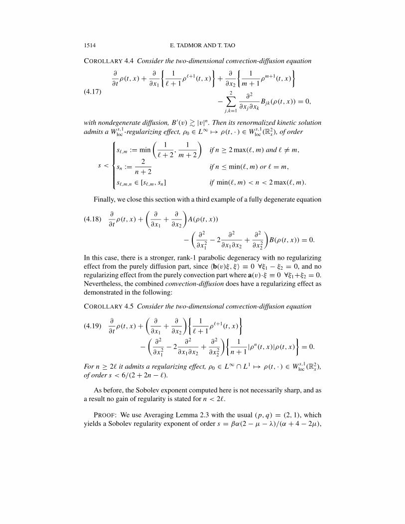
1514 E. TADMOR AND T. TAO
COROLLARY 4.4 Consider the two-dimensional convection-diffusion equation
∂
∂tρ(t, x) + ∂
∂x1
{1
� + 1ρ�+1(t, x)
}+ ∂
∂x2
{1
m + 1ρm+1(t, x)
}−
2∑j,k=1
∂2
∂xj∂xkBjk(ρ(t, x)) = 0,
(4.17)
with nondegenerate diffusion, B ′(v) � |v|n. Then its renormalized kinetic solutionadmits a W s,1
loc -regularizing effect, ρ0 ∈ L∞ �→ ρ(t, · ) ∈ W s,1loc (R2
x), of order
s <
s�,m := min
(1
� + 2,
1
m + 2
)if n ≥ 2 max(�, m) and � �= m,
sn := 2
n + 2if n ≤ min(�, m) or � = m,
s�,m,n ∈ [s�,m, sn] if min(�, m) < n < 2 max(�, m).
Finally, we close this section with a third example of a fully degenerate equation
(4.18)∂
∂tρ(t, x) +
(∂
∂x1
+ ∂
∂x2
)A(ρ(t, x))
−(
∂2
∂x21
− 2∂2
∂x1∂x2
+ ∂2
∂x22
)B(ρ(t, x)) = 0.
In this case, there is a stronger, rank-1 parabolic degeneracy with no regularizing
effect from the purely diffusion part, since 〈b(v)ξ, ξ〉 ≡ 0 ∀ξ1 − ξ2 = 0, and no
regularizing effect from the purely convection part where a(v)·ξ ≡ 0 ∀ξ1+ξ2 = 0.
Nevertheless, the combined convection-diffusion does have a regularizing effect as
demonstrated in the following:
COROLLARY 4.5 Consider the two-dimensional convection-diffusion equation
(4.19)∂
∂tρ(t, x) +
(∂
∂x1
+ ∂
∂x2
){1
� + 1ρ�+1(t, x)
}−
(∂2
∂x21
− 2∂2
∂x1∂x2
+ ∂2
∂x22
){1
n + 1|ρn(t, x)|ρ(t, x)
}= 0.
For n ≥ 2� it admits a regularizing effect, ρ0 ∈ L∞ ∩ L1 �→ ρ(t, · ) ∈ W s,1loc (R2
x),of order s < 6/(2 + 2n − �).
As before, the Sobolev exponent computed here is not necessarily sharp, and as
a result no gain of regularity is stated for n < 2�.
PROOF: We use Averaging Lemma 2.3 with the usual (p, q) = (2, 1), which
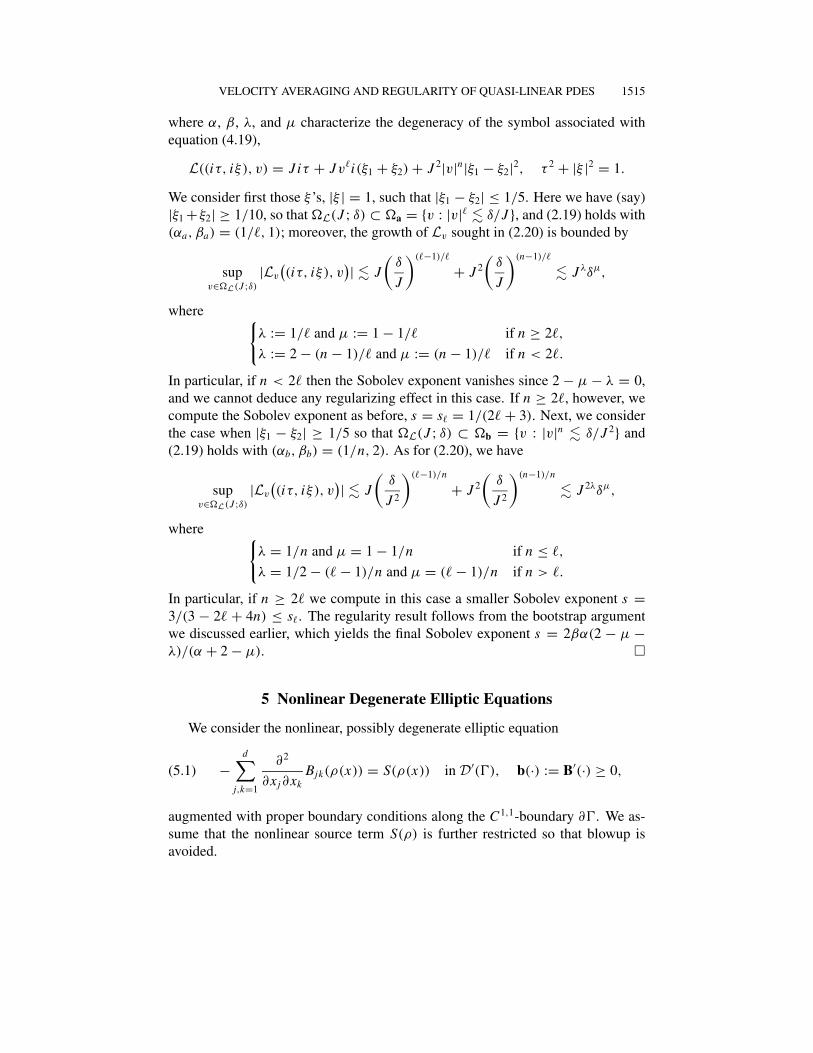
yields a Sobolev regularity exponent of order s = βα(2 − µ − λ)/(α + 4 − 2µ),
VELOCITY AVERAGING AND REGULARITY OF QUASI-LINEAR PDES 1515
where α, β, λ, and µ characterize the degeneracy of the symbol associated with
equation (4.19),
L((iτ, iξ), v) = J iτ + Jv�i(ξ1 + ξ2) + J 2|v|n|ξ1 − ξ2|2, τ 2 + |ξ |2 = 1.
We consider first those ξ ’s, |ξ | = 1, such that |ξ1 − ξ2| ≤ 1/5. Here we have (say)
|ξ1 + ξ2| ≥ 1/10, so that �L(J ; δ) ⊂ �a = {v : |v|� � δ/J }, and (2.19) holds with
(αa, βa) = (1/�, 1); moreover, the growth of Lv sought in (2.20) is bounded by
supv∈�L(J ;δ)
|Lv
((iτ, iξ), v
)| � J
(δ
J
)(�−1)/�
+ J 2
(δ
J
)(n−1)/�
� J λδµ,
where {λ := 1/� and µ := 1 − 1/� if n ≥ 2�,
λ := 2 − (n − 1)/� and µ := (n − 1)/� if n < 2�.
In particular, if n < 2� then the Sobolev exponent vanishes since 2 − µ − λ = 0,
and we cannot deduce any regularizing effect in this case. If n ≥ 2�, however, we
compute the Sobolev exponent as before, s = s� = 1/(2� + 3). Next, we consider
the case when |ξ1 − ξ2| ≥ 1/5 so that �L(J ; δ) ⊂ �b = {v : |v|n � δ/J 2} and
(2.19) holds with (αb, βb) = (1/n, 2). As for (2.20), we have
supv∈�L(J ;δ)
|Lv
((iτ, iξ), v
)| � J
(δ
J 2
)(�−1)/n
+ J 2
(δ
J 2
)(n−1)/n
� J 2λδµ,
where {λ = 1/n and µ = 1 − 1/n if n ≤ �,
λ = 1/2 − (� − 1)/n and µ = (� − 1)/n if n > �.
In particular, if n ≥ 2� we compute in this case a smaller Sobolev exponent s =3/(3 − 2� + 4n) ≤ s�. The regularity result follows from the bootstrap argument
we discussed earlier, which yields the final Sobolev exponent s = 2βα(2 − µ −λ)/(α + 2 − µ). �
5 Nonlinear Degenerate Elliptic Equations
We consider the nonlinear, possibly degenerate elliptic equation
(5.1) −d∑
j,k=1
∂2
∂xj∂xkBjk(ρ(x)) = S(ρ(x)) in D
′(�), b(·) := B′(·) ≥ 0,
augmented with proper boundary conditions along the C1,1-boundary ∂�. We as-
sume that the nonlinear source term S(ρ) is further restricted so that blowup is
avoided.
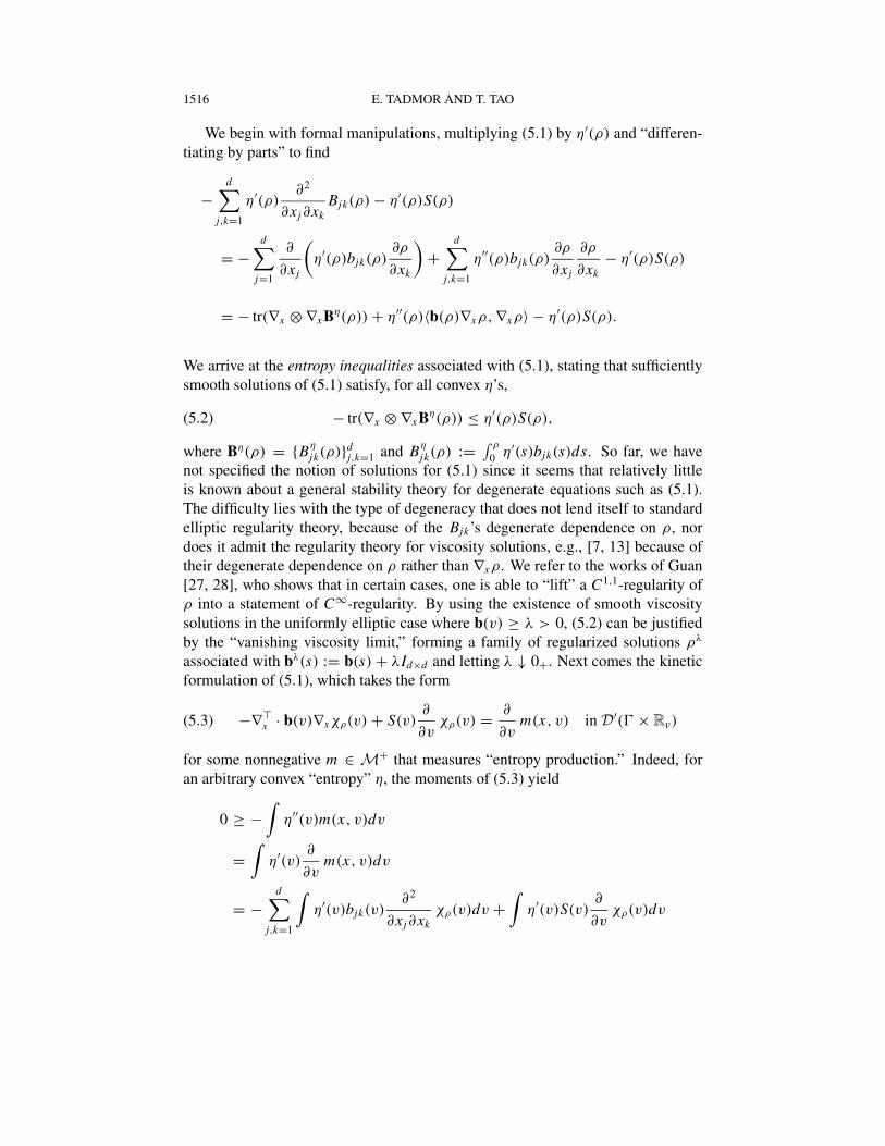
1516 E. TADMOR AND T. TAO
We begin with formal manipulations, multiplying (5.1) by η′(ρ) and “differen-
tiating by parts” to find
−d∑
j,k=1
η′(ρ)∂2
∂xj∂xkBjk(ρ) − η′(ρ)S(ρ)
= −d∑
j=1
∂
∂xj
(η′(ρ)bjk(ρ)
∂ρ
∂xk
)+
d∑j,k=1
η′′(ρ)bjk(ρ)∂ρ
∂xj
∂ρ
∂xk− η′(ρ)S(ρ)
= − tr(∇x ⊗ ∇x Bη(ρ)) + η′′(ρ)〈b(ρ)∇xρ, ∇xρ〉 − η′(ρ)S(ρ).
We arrive at the entropy inequalities associated with (5.1), stating that sufficiently
smooth solutions of (5.1) satisfy, for all convex η’s,
(5.2) − tr(∇x ⊗ ∇x Bη(ρ)) ≤ η′(ρ)S(ρ),
where Bη(ρ) = {Bη
jk(ρ)}dj,k=1 and Bη
jk(ρ) := ∫ ρ
0η′(s)bjk(s)ds. So far, we have
not specified the notion of solutions for (5.1) since it seems that relatively little
is known about a general stability theory for degenerate equations such as (5.1).
The difficulty lies with the type of degeneracy that does not lend itself to standard
elliptic regularity theory, because of the Bjk’s degenerate dependence on ρ, nor
does it admit the regularity theory for viscosity solutions, e.g., [7, 13] because of
their degenerate dependence on ρ rather than ∇xρ. We refer to the works of Guan
[27, 28], who shows that in certain cases, one is able to “lift” a C1,1-regularity of
ρ into a statement of C∞-regularity. By using the existence of smooth viscosity
solutions in the uniformly elliptic case where b(v) ≥ λ > 0, (5.2) can be justified
by the “vanishing viscosity limit,” forming a family of regularized solutions ρλ
associated with bλ(s) := b(s) + λId×d and letting λ ↓ 0+. Next comes the kinetic
formulation of (5.1), which takes the form
(5.3) −∇�x · b(v)∇xχρ(v) + S(v)
∂
∂vχρ(v) = ∂
∂vm(x, v) in D
′(� × Rv)
for some nonnegative m ∈ M+ that measures “entropy production.” Indeed, for
an arbitrary convex “entropy” η, the moments of (5.3) yield
0 ≥ −∫
η′′(v)m(x, v)dv
=∫
η′(v)∂
∂vm(x, v)dv
= −d∑
j,k=1
∫η′(v)bjk(v)
∂2
∂xj∂xkχρ(v)dv +
∫η′(v)S(v)
∂
∂vχρ(v)dv
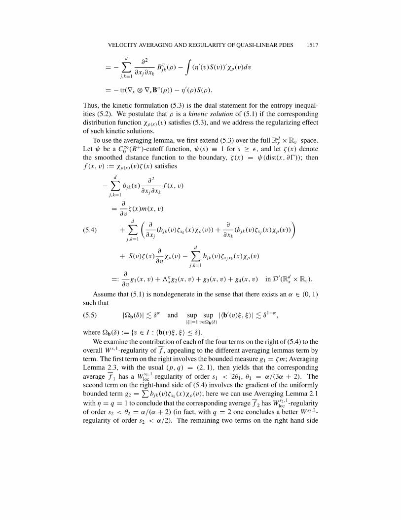
VELOCITY AVERAGING AND REGULARITY OF QUASI-LINEAR PDES 1517
= −d∑
j,k=1
∂2
∂xj∂xkBη
jk(ρ) −∫
(η′(v)S(v))′χρ(v)dv
= − tr(∇x ⊗ ∇x Bη(ρ)) − η′(ρ)S(ρ).
Thus, the kinetic formulation (5.3) is the dual statement for the entropy inequal-
ities (5.2). We postulate that ρ is a kinetic solution of (5.1) if the corresponding
distribution function χρ(x)(v) satisfies (5.3), and we address the regularizing effect
of such kinetic solutions.
To use the averaging lemma, we first extend (5.3) over the full Rdx × Rv–space.
Let ψ be a C∞0 (R+)-cutoff function, ψ(s) ≡ 1 for s ≥ ε, and let ζ(x) denote
the smoothed distance function to the boundary, ζ(x) = ψ(dist(x, ∂�)); then
f (x, v) := χρ(x)(v)ζ(x) satisfies
−d∑
j,k=1
bjk(v)∂2
∂xj∂xkf (x, v)
= ∂
∂vζ(x)m(x, v)
+d∑
j,k=1
(∂
∂xj(bjk(v)ζxk (x)χρ(v)) + ∂
∂xk(bjk(v)ζxj (x)χρ(v))
)
+ S(v)ζ(x)∂
∂vχρ(v) −
d∑j,k=1
bjk(v)ζxj xk (x)χρ(v)
=: ∂
∂vg1(x, v) + η
x g2(x, v) + g3(x, v) + g4(x, v) in D′(Rd
x × Rv).
(5.4)
Assume that (5.1) is nondegenerate in the sense that there exists an α ∈ (0, 1)
such that
(5.5) |�b(δ)| � δα and sup|ξ |=1
supv∈�b(δ)
|〈b′(v)ξ, ξ〉| � δ1−α,
where �b(δ) := {v ∈ I : 〈b(v)ξ, ξ〉 ≤ δ}.We examine the contribution of each of the four terms on the right of (5.4) to the
overall W s,1-regularity of f , appealing to the different averaging lemmas term by
term. The first term on the right involves the bounded measure g1 = ζm; Averaging
Lemma 2.3, with the usual (p, q) = (2, 1), then yields that the corresponding
average f 1 has a W s1,1loc -regularity of order s1 < 2θ1, θ1 = α/(3α + 2). The
second term on the right-hand side of (5.4) involves the gradient of the uniformly
bounded term g2 = ∑bjk(v)ζxk (x)χρ(v); here we can use Averaging Lemma 2.1
with η = q = 1 to conclude that the corresponding average f 2 has W s2,1loc -regularity
of order s2 < θ2 = α/(α + 2) (in fact, with q = 2 one concludes a better W s2,2-
regularity of order s2 < α/2). The remaining two terms on the right-hand side
1518 E. TADMOR AND T. TAO
of (5.4) yield smoother averages and therefore do not affect the overall regularity
dictated by the first two. Indeed, ∂vχρ(v) and hence g3(x, v) = S(v)ζ(x)∂vχρ(v)
is a bounded measure, and Averaging Lemma 2.1 with η = N = 0 implies that
the corresponding average f 3 belongs to the smaller Sobolev space W s3,1loc of order
s3 < 2θ3, θ3 = α/(α + 2). Finally, the last term on the right of (5.4) consists of
the bounded sum, g4 = −∑bjk(v)ζxj xk (x)χρ ; with η = N = 0 and q = 2, the
corresponding average f 4 has a W s4,2loc -regularity of order s4 < 2θ4, θ4 = α/2.
Next, we iterate the bootstrap argument we mentioned earlier in the context of
hyperbolic conservation laws. The first W s1,1-bound together with the L∞-bound
of f imply a W σ1,2loc -bound with σ1 = s1/2, which in turn yields the improved
regularity of f 1 ∈ W s,1loc , s < (1 − θ1)σ1 + 2θ1. Thus, for the first term we can
iterate the improved regularity, s1 �→ (1 − θ1)s1/2 + 2θ1, converging to the same
fixed point we had in the parabolic case before, s1 < 2α/(2α + 1). The second
term requires a more careful treatment: as we iterate the improved regularity of
χρ ∈ W s,1loc , we can express the term on the right of (5.4) as ηs g2 with ηs := 1 − s
and with g2 standing for the sum of L1-bounded terms, g2 = s∑
bjk(v)ζxk χρ(v).
Consequently, Averaging Lemma 2.1 yields the fixed-point iterations s2 �→ (1 −θ2)s2/2 + (2 − ηs2
)θ2 with limiting regularity of order s2 < α. The remaining two
terms are smoother and do not affect the overall regularity: a similar argument for
the third term yields the fixed-point iterations, s3 �→ (1−θ3)s3/2+2θ3 with a fixed
point s3 < 2α/(α + 1), while the fourth term remains in the smaller Sobolev space
W α,2. We summarize with the following statement:
COROLLARY 5.1 Let ρ ∈ L∞ be a kinetic solution of the nonlinear elliptic equa-tion (5.1) and assume the nondegeneracy condition (5.5) holds. Then we have theinterior regularity estimate for all D ⊂ �,
ρ(x) ∈ W s,1loc (D), s <
α if α < 12,
2α
2α + 1if 1
2< α < 1.
Acknowledgments. Part of this research was carried out while E.T. was visiting
the Weizmann Institute for Science, and it is a pleasure to thank the faculty of math-
ematics and computer science for their hospitality. Research was supported in part
by National Science Foundation Grant DMS #DMS04-07704 and ONR #N00014-
91-J-1076 (E.T.) and by the David and Lucille Packard Foundation (T.T.).
Bibliography
[1] Agoshkov, V. I. Spaces of functions with differential-difference characteristics and the smooth-
ness of solutions of the transport equation. Dokl. Akad. Nauk SSSR 276 (1984), no. 6, 1289–
1293; translation in Soviet Math. Dokl. 29 (1984), no. 3, 662–666.
[2] Bénilan, P.; Crandall, M. G. The continuous dependence on ϕ of solutions of ut − �ϕ(u) = 0.
Indiana Univ. Math. J. 30 (1981), no. 2, 161–177.
VELOCITY AVERAGING AND REGULARITY OF QUASI-LINEAR PDES 1519
[3] Bénilan, P.; Crandall, M. G. Regularizing effects of homogeneous evolution equations. Con-tributions to analysis and geometry (Baltimore, Md., 1980), 23–39. Johns Hopkins University
Press, Baltimore, Md., 1981.
[4] Bézard, M. Régularité L p précisée des moyennes dans les équations de transport. Bull. Soc.Math. France 122 (1994), no. 1, 29-76.
[5] Bouchut, F.; Desvillettes, L. Averaging lemmas without time Fourier transform and application
to discretized kinetic equations. Proc. Roy. Soc. Edinburgh Sect. A 129 (1999), no. 1, 19–36.
[6] Brézis, H.; Crandall, M. G. Uniqueness of solutions of the initial-value problem for ut −�ϕ(u) = 0. J. Math. Pures Appl. (9) 58 (1979), no. 2, 153–163.
[7] Caffarelli, L. A.; Cabré, X. Fully nonlinear elliptic equations. American Mathematical Society
Colloquium Publications, 43. American Mathematical Society, Providence, R.I., 1995.
[8] Carrillo, J. Entropy solutions for nonlinear degenerate problems. Arch. Ration. Mech. Anal. 147
(1999), no. 4, 269–361.
[9] Chen, G.-Q. Some recent methods for partial differential equations of divergence form. Dedi-
cated to the 50th anniversary of IMPA. Bull. Braz. Math. Soc. (N.S.) 34 (2003), no. 1, 107–144.
[10] Chen, G.-Q.; Karlsen, K. H. L1-framework for continuous dependence and error estimates for
quasilinear anisotropic degenerate parabolic equations. Trans. Amer. Math. Soc. 358 (2006),
no. 3, 937–963 (electronic).
[11] Chen, G.-Q.; Perthame, B. Well-posedness for non-isotropic degenerate parabolic-hyperbolic
equations. Ann. Inst. H. Poincaré Anal. Non Linéaire 20 (2003), no. 4, 645–668.
[12] Cheverry, C. Regularizing effects for multidimensional scalar conservation laws. Ann. Inst.H. Poincaré Anal. Non Linéaire 17 (2000), no. 4, 413–472.
[13] Crandall, M. G.; Ishii, H.; Lions, P.-L. User’s guide to viscosity solutions of second order partial
differential equations. Bull. Amer. Math. Soc. (N.S.) 27 (1992), no. 1, 1–67.
[14] Crandall, M. G.; Kocan, M.; Lions, P. L.; Swiech, A. Existence results for boundary problems
for uniformly elliptic and parabolic fully nonlinear equations. Electron. J. Differential Equa-tions 1999, no. 24, 22 pp. (electronic).
[15] De Lellis, C.; Westdickenberg, M. On the optimality of velocity averaging lemmas. Ann. Inst.H. Poincaré Anal. Non Linéaire 20 (2003), no. 6, 1075–1085.
[16] DeVore, R.; Petrova, G. The averaging lemma. J. Amer. Math. Soc. 14 (2001), no. 2, 279–296
(electronic).
[17] DiBenedetto, E. Degenerate parabolic equations. Universitext. Springer, New York, 1993.
[18] DiPerna, R. J.; Lions, P.-L. Global weak solutions of Vlasov-Maxwell systems. Comm. PureAppl. Math. 42 (1989), no. 6, 729–757.
[19] DiPerna, R. J.; Lions, P.-L. On the Cauchy problem for Boltzmann equations: global existence
and weak stability. Ann. of Math. (2) 130 (1989), no. 2, 321–366.
[20] DiPerna, R. J.; Lions, P.-L.; Meyer, Y. L p regularity of velocity averages. Ann. Inst. H. PoincaréAnal. Non Linéaire 8 (1991), no. 3-4, 271–287.
[21] Engquist, B.; E, W. Large time behavior and homogenization of solutions of two-dimensional
conservation laws. Comm. Pure Appl. Math. 46 (1993), no. 1, 1–26.
[22] Gérard, P. Moyennisation et régularité deux-microlocale. Ann. Sci. École Norm. Sup. (4) 23
(1990), no. 1, 89–121.
[23] Gérard, P.; Golse, F. Averaging regularity results for PDEs under transversality assumptions.
Comm. Pure Appl. Math. 45 (1992), no. 1, 1–26.
[24] Golse, F.; Lions, P.-L.; Perthame, B.; Sentis, R. Regularity of the moments of the solution of a
transport equation. J. Funct. Anal. 76 (1988), no. 1, 110–125.
[25] Golse, F.; Perthame, B.; Sentis, R. Un résultat de compacité pour les équations de transport
et application au calcul de la limite de la valeur propre principale d’un opérateur de transport.
C. R. Acad. Sci. Paris Sér. I Math. 301 (1985), no. 7, 341–344.
1520 E. TADMOR AND T. TAO
[26] Golse, F.; Saint-Raymond, L. Velocity averaging in L1 for the transport equation. C. R. Math.Acad. Sci. Paris 334 (2002), no. 7, 557–562.
[27] Guan, P. Regularity of a class of quasilinear degenerate elliptic equations. Adv. Math. 132
(1997), no. 1, 24–45.
[28] Guan, P. Nonlinear degenerate elliptic equations. Proceedings of ICCM2001 (Taiwan, 2001),257–266. New Studies in Advanced Mathematics, 4. International, Somerville, Mass., 2004.
Available online at http://www.math.mcgill.ca/guan/iccm.dvi
[29] Jabin, P.-E.; Perthame, B. Regularity in kinetic formulations via averaging lemmas. A tribute to
J. L. Lions. ESAIM Control Optim. Calc. Var. 8 (2002), 761–774 (electronic).
[30] Jabin, P.-E.; Vega, L. Averaging lemmas and the X-ray transform. C. R. Math. Acad. Sci. Paris337 (2003), no. 8, 505–510.
[31] Jabin, P.-E.; Vega, L. A real space method for averaging lemmas. J. Math. Pures Appl. (9) 83
(2004), no. 11, 1309–1351.
[32] Kružkov, S. N. First order quasilinear equations in several independent variables. Mat. Sb. (N.S.)81 (1970), no. 123, 228–255.
[33] Lax, P. D. Hyperbolic systems of conservation laws and the mathematical theory of shockwaves. Conference Board of the Mathematical Sciences Regional Conference Series in Applied
Mathematics, 11. Society for Industrial and Applied Mathematics, Philadelphia, 1973.
[34] Lions, P.-L. Régularité optimale des moyennes en vitesses. C. R. Acad. Sci. Paris Sér. I Math.
320 (1995), no. 8, 911–915.
[35] Lions, P.-L.; Perthame, B.; Souganidis, P. E. Existence and stability of entropy solutions for the
hyperbolic systems of isentropic gas dynamics in Eulerian and Lagrangian coordinates. Comm.Pure Appl. Math. 49 (1996), no. 6, 599–638.
[36] Lions, P.-L.; Perthame, B.; Tadmor, E. A kinetic formulation of multidimensional scalar con-
servation laws and related equations. J. Amer. Math. Soc. 7 (1994), no. 1, 169–191.
[37] Lions, P.-L.; Perthame, B.; Tadmor, E. Kinetic formulation of the isentropic gas dynamics and
p-systems. Comm. Math. Phys. 163 (1994), no. 2, 415–431.
[38] Oleınik, O. A. Discontinuous solutions of non-linear differential equations. Amer. Math. Soc.Transl. (2) 26 (1963), 95–172.
[39] Perthame, B. Kinetic formulation of conservation laws. Oxford Lecture Series in Mathematics
and Its Applications, 21. Oxford University Press, Oxford, 2002.
[40] Perthame, B. Mathematical tools for kinetic equations. Bull. Amer. Math. Soc. (N.S.) 41 (2004),
no. 2, 205–244.
[41] Perthame, B.; Souganidis, P. E. A limiting case for velocity averaging. Ann. Sci. École Norm.Sup. (4) 31 (1998), no. 4, 591–598.
[42] Perthame, B.; Souganidis, P. E Dissipative and entropy solutions to non-isotropic degenerate
parabolic balance laws. Arch. Ration. Mech. Anal. 170 (2003), no. 4, 359–370.
[43] Perthame, B.; Tadmor, E. A kinetic equation with kinetic entropy functions for scalar conser-
vation laws. Comm. Math. Phys. 136 (1991), no. 3, 501–517.
[44] Stein, E. M. Harmonic analysis: real-variable methods, orthogonality, and oscillatory inte-grals. Princeton Mathematical Series, 43. Monographs in Harmonic Analysis, 3. Princeton
University Press, Princeton, N.J., 1993.
[45] Tadmor, E.; Rascle, M.; Bagnerini, P. Compensated compactness for 2D conservation laws.
J. Hyperbolic Differ. Equ. 2 (2005), no. 3, 697–712.
[46] Tartar, L. Compensated compactness and applications to partial differential equations. Non-linear analysis and mechanics: Heriot-Watt Symposium, vol. 4, 136–212. Research Notes in
Mathematics, 39. Pitman, Boston–London, 1979.
[47] Tartar, L. The compensated compactness method for a scalar hyperbolic equation. Lecture
notes, 87-20. Carnegie-Mellon University, Pittsburgh, Pa., 1987.
VELOCITY AVERAGING AND REGULARITY OF QUASI-LINEAR PDES 1521
[48] Tartar, L. H -measures, a new approach for studying homogenisation, oscillations and concen-
tration effects in partial differential equations. Proc. Roy. Soc. Edinburgh Sect. A 115 (1990),
no. 3-4, 193–230.
[49] Tartar, L. An introduction to Sobolev spaces and interpolation spaces. Available online at
http://www.math.cmu.edu/cna/publications.html/SOB+Int.pdf
[50] Tassa, T. Regularity of weak solutions of the nonlinear Fokker-Planck equation. Math. Res.Lett. 3 (1996), no. 4, 475–490.
[51] Tassa, T. Uniqueness of piecewise smooth weak solutions of multidimensional degenerate par-
abolic equations. J. Math. Anal. Appl. 210 (1997), no. 2, 598–608.
[52] Vasseur, A. Kinetic semidiscretization of scalar conservation laws and convergence by using
averaging lemmas. SIAM J. Numer. Anal. 36 (1999), no. 2, 465–474 (electronic).
[53] Vol′pert, A. I.; Hudjaev, S. I. The Cauchy problem for second order quasilinear degenerate
parabolic equations. Mat. Sb. (N.S.) 78 (120) (1969), 374–396; translation in Math. USSR-Sb.
7 (1969), no. 3, 365–387.
[54] Westdickenberg, M. Some new velocity averaging results. SIAM J. Math. Anal. 33 (2002),
no. 5, 1007–1032 (electronic).
EITAN TADMOR TERENCE TAO
University of Maryland UCLA
Department of Mathematics Department of Mathematics
CSCAMM, 4149 CSIC Building #406 Box 951555
Paint Branch Drive Los Angeles, CA 90095-1555
College Park, MD 20742-2389 E-mail: [email protected]
E-mail: tadmor@
cscamm.umd.edu
Received November 2005.


![Regularizing AdaBoostpapers.nips.cc/paper/1615-regularizing-adaboost.pdfBoosting and other ensemble methods have been used with success in several ap plications, e.g. OCR [13, 8]](https://img.pdfslide.us/doc/110x75/5f49758b79a6cc2793298b7e/regularizing-boosting-and-other-ensemble-methods-have-been-used-with-success-in.jpg)