LINEAR IDENTIFICATION AND CONTROL OF REACTOR FOR PHTHALIC ... /Archive-2016/October-2016/73.pdf · LINEAR IDENTIFICATION AND CONTROL OF REACTOR FOR PHTHALIC ANHYDRIDE PRODUCTION PROCESS

ISSN: 2277-9655

[Malathi* et al., 5(10): October, 2016] Impact Factor: 4.116

IC™ Value: 3.00 CODEN: IJESS7

http: // www.ijesrt.com © International Journal of Engineering Sciences & Research Technology

[601]

IJESRT INTERNATIONAL JOURNAL OF ENGINEERING SCIENCES & RESEARCH

TECHNOLOGY

LINEAR IDENTIFICATION AND CONTROL OF REACTOR FOR PHTHALIC

ANHYDRIDE PRODUCTION PROCESS - CASE STUDY S. Malathi*, N. S. Bhuvanewswari

* Dept of EIE Easwari Engineering College Ramapuram, Chennai – 600089. Tamilnadu, India

DOI: 10.5281/zenodo.163029

ABSTRACT Phthalic anhydride is one of the most essential and rare chemicals used in manufacturing of paints, pigments, dyes

and esters. Now a day, the demand for the purest form of Phthalic anhydride is increasing but the production is

low to meet the demand. Phthalic anhydride is produced by maintaining the constant ratio of air and ortho xylene

at 3:1 at very high temperature in mixing column. The mixture is passed through the reactor for reaction with

catalyst. Finally, it enters the switch condenser for product separation. The main problem is if the reactor is not

maintained below its critical value, leads to explosion. As feed material is a petroleum product, the energy released

is enormous, it can endanger the life of employees and to surroundings. For efficient control, linear and nonlinear

model identification using AR, ARX and ARMAX is done and conventional controller is included to operate the

plant in closed loop.

KEYWORDS: Phthalic Anhydride, Nonlinear model Identification, AR, ARX, ARMAX

INTRODUCTION Most of the industrial chemical processes are exothermic, it is essential to ensure protection and safety of the

operating personnel as well as the environment.As the reaction proceeds, the amount of heat generated will

increase.To achieve the desired product, it is necessary to maintain the process temperature at the required value.

Properknowledge on type, ratio of the raw materials added, catalysts used, surrounding and reacting conditions is

required to carry out process in efficient and controlled manner.Phthalic anhydride is used in manufacture of

paints, esters, dies, pigments etc.Production of phthalic anhydride is an exothermic process, where the amount of

heat generated is high. The reaction exothermic as the medium in which the reaction is taking place gains heat.

When the increased amount of heat is not compensated by the jacket coolant temperature, reactor cracks and

thermal explosion occurs. Thermodynamics and kinetics of the chemical reactions determines the design of the

reactor. Batch and continuous type reactors are available. Batch reactors are mainly used in laboratories where

the reactants are placed in a test-tube, beaker. Reactants are mixed together and heated for the reaction to take

place. Finally, after reaction the mixture is cooled and purified based on requirements.Alternatively, the reactants

are fed continuously into the reactor at one point. The products are withdrawn at another point after the reaction

completes.In a continuous reactor, steady state must be attained where the flow rate into the reactor equal the flow

rates out of the reactor, or else the tank would be empty or overflow. By dividing the volume of the tank by the

average volumetric flow rate the residence time is calculated .Instead of calculating absolute amount of energy,

enthalpy change is calculated as it is easier. The work needed to change the volume of the system against ambient

pressure plus the change in internal energy of the system calculates the enthalpy change. World demand for PA

is expected to start recovering in 2010-2012, largely as a result of improved activity in the construction,

automotive and original equipment manufacture (OEM) sectors. US-based consultant orecasts world

consumption to grow at an average rate of 2.8%/year during the 2009-2014 period. However, this growth is

expected to vary greatly by application and region. Phthalic anhydride is the organic compound with the formula

C6H4(CO)2O, anhydride of phthalic acid of formula C6H4(CO2H)2 and an isomer of iso-phthalic acid.

Commercially, it is anhydride of dicarboxylic acid. Phthalic anhydride is a colorless solid is an important industrial

chemical. It is used for the large scale production of plastics. Market survey dictates the maximum usage of pthalic

anhydride is in the manufacture of phthalate plasticisers which is used as a plasticiser in polyvinyl chloride (PVC).

The major consumption of PA is mainly dependent on the growth of PVC, which is sensitive to general economic

http://www.ijesrt.com/

ISSN: 2277-9655




[602]

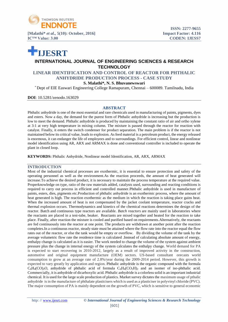
conditions as it is consumed mainly in the construction and automobile industries. Fig.1. shows the structure of

phthalic anhydride.

Figure:

Fig.1.Structure of Phthalic anhydride

The primary preparation for the process starts with mixture of air and ortho-xylene. Air is uncontrolled stream

and ortho-xylene is controlled stream. Ortho-xylene is scarce feed material so it must be used efficiently. For

initial startup of the reaction air must be preheated to 937oC. Then air is mixed in a desired ratio with ortho-xylene

which is at room temperature.

The mixture is feed to the reactor for the reaction to take place. Before that the reaction mixture must be preheated

because the required temperature for the reaction is very high and it requires more energy and more time for

reactor to attain the temperature and the efficiency also reduces. The reaction temperature is 535oC. So the jacket

heat flow must be regulated in the way to maintain the reaction temperature. After that it has to pass through

switch condenser for separation of immiscible solid particles in product. Then it must pass through the distillation

column for separation of low temperature and high temperature products. The purity of the material is an important

factor in this reaction. For that temperature has to be maintained. Along with the coolant temperature also

measured for more efficient control in the phthalic anhydride process.There is difficulty in maintaining the

reaction because this reaction highly exothermic. The reaction must be triggered for quick formation of phthalic

acid. For that a solid catalyst Vanadium Pentoxide (V2O5) is added. At 535oC only the catalyst reacts with the

mixture to form phthalic acid. But when the time when the catalyst and mixture starts to react then the reaction

turns into highly exothermic reaction and becomes difficult to control. The control action is taken but with large

delay in time. The product which are formed between the temperature range 534oC and 537oC are considered as

the best quality raw material. But the quantity at that range of temperature is very low but the demand for the

quality and quantity is increasing day by day.

IDENTIFICATION Method of identifying the mathematical model of a system from measurements of the process inputs and outputs

is termed as system identification. System identification for nonlinear is developed based on four basic

approaches, Volterra Series Models, Block Structured Models, Neural Network Models, and NARMAX Models.

Volterra Series Modelis a model defined for non-linear behaviour. The input to the process at all other times

defines the output of the non-linear process in volterra series model. Block structured model is nothing but

Hammerstein - Wiener model. In Hammerstein model, a linear dynamic element is considered after static single

valued non-linear element. In Wiener model, the linear element occurs before the static nonlinear characteristic.

Generally,a static linear element sandwiched between two dynamic systems is known as Hammerstein – Wiener

model. Nonlinear Auto Regressive Moving Averagewith Exogenousinput model (NARMAX) consists of past

inputs, outputs and noise terms. Unbiased estimates of the system model can be obtained because the noise is

modelled explicitly in the presence of nonlinear noise and unobserved highly correlated.

Dynamic model that connects the excited inputs with measured outputs is identified by using different model

structures. Model structures include unknown parameters inside the model. Set of criteria functions are chosen to

determine best model structure. Transfer function model, polynomial models like AR, ARX and ARMAX models

are discussed.

Transfer function Model


http://en.wikipedia.org/wiki/Mathematical_model

http://en.wikipedia.org/wiki/System

ISSN: 2277-9655




[603]

Transfer function is a function that relates input and output is known as transfer function. Reference input

operates through transfer function. Input operating with the function of the process produces an effect resulting

in controlled output or response. Thus, a transfer function provides cause and effect relationship between

input and output.

𝐺(𝑆) = 𝐶(𝑆)

𝑅(𝑆) (1)

A. AR Model

Auto Regressive model is a type of polynomial model. AR model parameters are estimated using variants of the

least-squares method where model structure is given by the following equation

𝐴(𝑞)𝑦(𝑡) = 𝑒(𝑡) (2)

B. ARX Model

Auto Regressive with Exogenous input also called as Controlled Autoregressive model. This structure is viewed

in linear regression. The ARX model structure is

𝑦(𝑡) + 𝑎1𝑦(𝑡 − 1) + ⋯ + 𝑎𝑛𝑎𝑦(𝑡 − 𝑛𝑎) = 𝑏1𝑢(𝑡 − 𝑛𝑘) + ⋯ + 𝑏𝑛𝑏𝑢(𝑡 − 𝑛𝑏 − 𝑛𝑘 + 1) + 𝑒(𝑡) (3)

C. ARMAX Model

Auto Regressive Moving Average with Exogenous input estimates the time domain data model. The model is

written explicitly as the difference equation

𝑦(𝑡) + 𝑎1𝑦(𝑡 − 1) + ⋯ + 𝑎𝑛𝑎𝑦(𝑡 − 𝑛𝑎) = 𝑏1𝑢(𝑡 − 1) + ⋯ + 𝑏𝑛𝑏𝑢(𝑡 − 𝑛𝑏) + 𝑐1𝑒(𝑡 − 1) + ⋯ + 𝑐𝑛𝑐𝑒(𝑡 −𝑛𝑐)(4)

CONTROL

Proportional-Integral-Derivative (PID) control is the most commonly used control algorithm in industry and is

universally accepted. The difference between a desired setpoint and a measured process variable is continuously

calculated to obtain the error value. The error is minimized by adjusting the control variable. The position of

a control valve, a damper is altered to reduce the error. The PID controller equation includes the proportional,

integral and derivative gains as shown in eqn (4).

𝑢(𝑡) = 𝐾𝑝𝑒(𝑡) + 𝐾𝑖 ∫ 𝑒(𝑡)𝑑𝑡 + 𝐾𝑑𝑑𝑒(𝑡)

𝑑𝑡

𝑡

0 (5)

P accounts for present values of the error, I accounts for past values of the error and D accounts for possible future

values of the error, based on its current rate of change.PID controller can deal with specific process requirements

if the three parameters of the controller are tuned.

A. Proportional term

Output of the proportional term is proportional to the current error value. A constant kpis adjusted to change the

response of the proportional term. The constant term is called the proportional gain constant.The proportional

term is given by

𝑃𝑜𝑢𝑡 = 𝐾𝑝 𝑒(𝑡) (6)

For a given change in the error, a large change in the output is obtained if the proportional gain is high. The

process becomes unstable if the proportional gain is too high. A small gain results in a small output response to a

large input error, and a less sensitive controller. The control action may be too small to process disturbances if the

proportional gain is too low.

B. Integral term

Output of the integral term is proportional to magnitude and the duration of the error. Sum of the instantaneous

error over time is provided by the integral term and provides the accumulated offset to be corrected previously.The

integral gain Kiis multiplied with the accumulated error and added to the controller output. The integral term is

given by

𝐼𝑜𝑢𝑡 = 𝐾𝑖 ∫ 𝑒(𝑡)𝑑𝑡𝑡

0 (7)

Residual steady-state error is eliminated with the integral part of PID controller. Residual steady-state error occurs

with a pure proportional controller. Present value overshoots from the setpoint value as the integral term response

depends on accumulated errors from the past.

C. Derivative term


https://en.wikipedia.org/wiki/Setpoint_(control_system)

https://en.wikipedia.org/wiki/Process_variable

https://en.wikipedia.org/wiki/Control_valve

https://en.wikipedia.org/wiki/Damper_(flow)

https://en.wikipedia.org/wiki/Overshoot_(signal)

ISSN: 2277-9655




[604]

Slope of the error over time is calculated to obtain the derivative of the process error. The error is multiplied with

the derivative gain Kd. The derivative term is given by:

𝐷𝑜𝑢𝑡 = 𝐾𝑑𝑑𝑒(𝑡)

𝑑𝑡 (8)

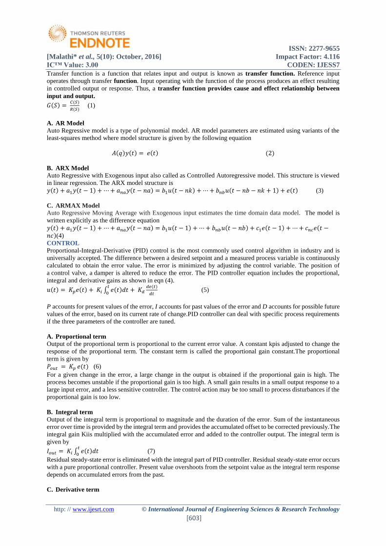
System behavior can be predicted from the derivative action thus settling time and stability of the process is

improved. Fig.2. shows the basic block diagram of the closed loop system used in the production of phthalic

anhydride process.

Figure:

Fig.2. Block diagram of Phthalic anhydride process

RESULTS AND DISCUSSION A. Model Identification

Transfer function Model

The transfer function of the process is estimated as the mathematical model for the process is not available. The

experimental data are collected and the transfer function for the process is determined by transfer function

estimation method in MATLAB. The input/output data is loaded in and object and then iddata object is created.

The initial conditions for the transfer function estimation are given. Then it is loaded in tfest function to give the

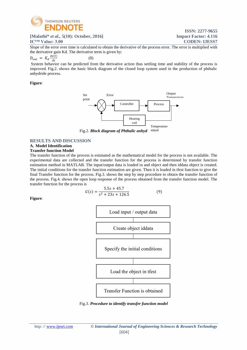
final Transfer function for the process. Fig.3. shows the step by step procedure to obtain the transfer function of

the process. Fig.4. shows the open loop response of the process obtained from the transfer function model. The

transfer function for the process is

𝐺(𝑠) =5.5𝑠 + 45.7

𝑠2 + 23𝑠 + 126.5 (9)

Figure:

Fig.3. Procedure to identify transfer function model

Load input / output data

Create object iddata

Specify the initial conditions

Load the object in tfest

Transfer Function is obtained

Controller Process

Heating

coil

Set

point

Error Output

Temperature

Temperature signal


ISSN: 2277-9655




[605]

Figure:

Fig.4.Response of the obtained transfer function

AR Model

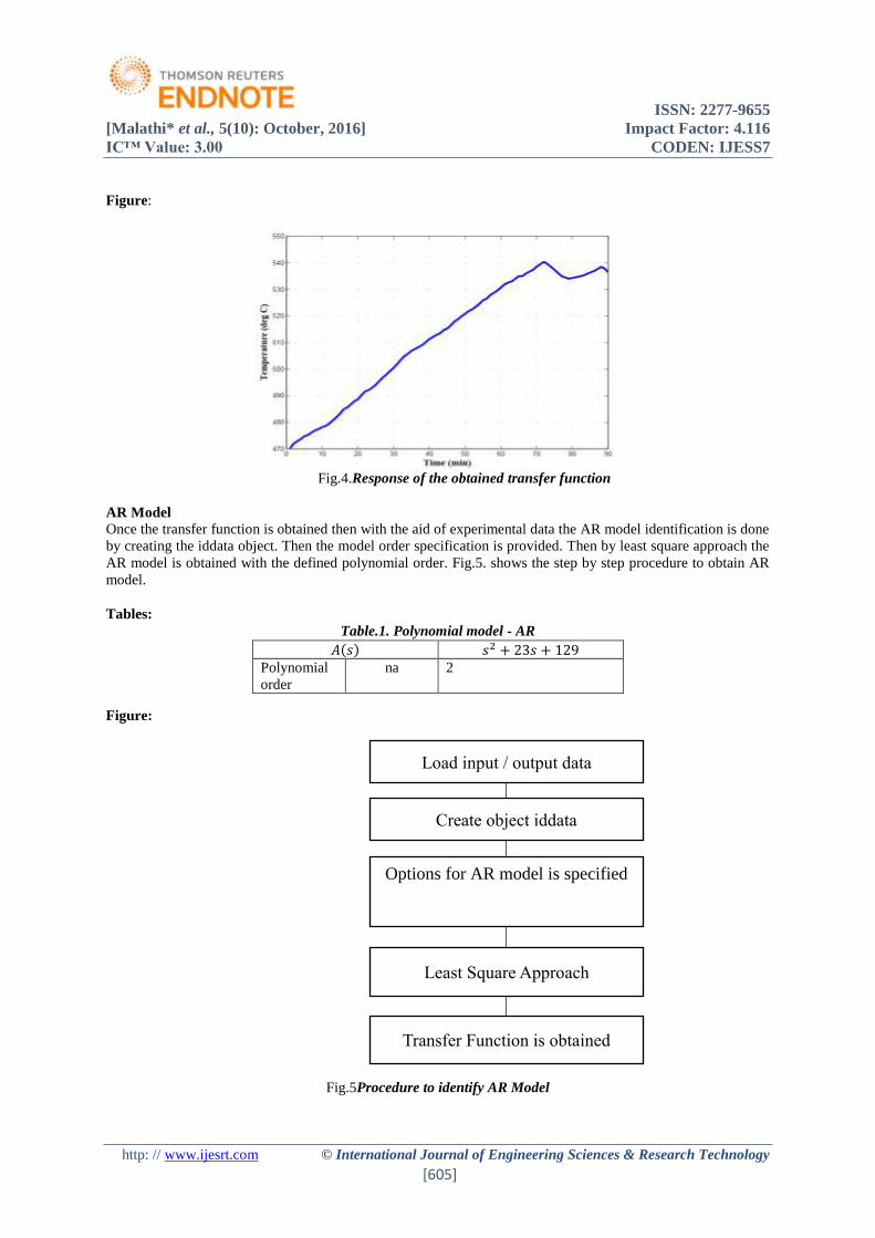
Once the transfer function is obtained then with the aid of experimental data the AR model identification is done

by creating the iddata object. Then the model order specification is provided. Then by least square approach the

AR model is obtained with the defined polynomial order. Fig.5. shows the step by step procedure to obtain AR

model.

Tables:

Table.1. Polynomial model - AR

Figure:

Fig.5Procedure to identify AR Model

𝐴(𝑠) 𝑠2 + 23𝑠 + 129

Polynomial

order

na 2



Options for AR model is specified

Least Square Approach



ISSN: 2277-9655




[606]

Table.1.

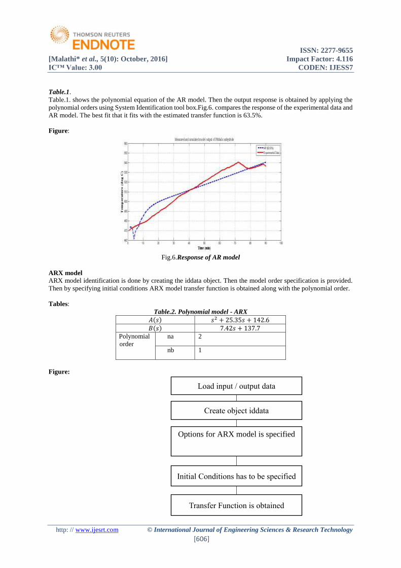
Table.1. shows the polynomial equation of the AR model. Then the output response is obtained by applying the

polynomial orders using System Identification tool box.Fig.6. compares the response of the experimental data and

AR model. The best fit that it fits with the estimated transfer function is 63.5%.

Figure:

Fig.6.Response of AR model

ARX model

ARX model identification is done by creating the iddata object. Then the model order specification is provided.

Then by specifying initial conditions ARX model transfer function is obtained along with the polynomial order.

Tables:

Table.2. Polynomial model - ARX

𝐴(𝑠) 𝑠2 + 25.35𝑠 + 142.6

𝐵(𝑠) 7.42𝑠 + 137.7

Polynomial

order

na 2

nb 1

Figure:



Options for ARX model is specified

Initial Conditions has to be specified



ISSN: 2277-9655




[607]

Fig.4 Procedure to identidy ARX model

Figure

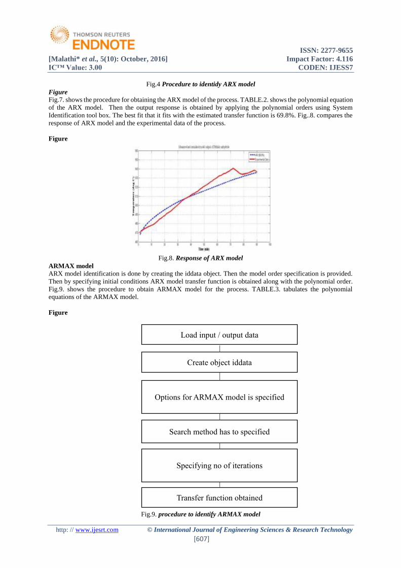
Fig.7. shows the procedure for obtaining the ARX model of the process. TABLE.2. shows the polynomial equation

of the ARX model. Then the output response is obtained by applying the polynomial orders using System

Identification tool box. The best fit that it fits with the estimated transfer function is 69.8%. Fig..8. compares the

response of ARX model and the experimental data of the process.

Figure

Fig.8. Response of ARX model

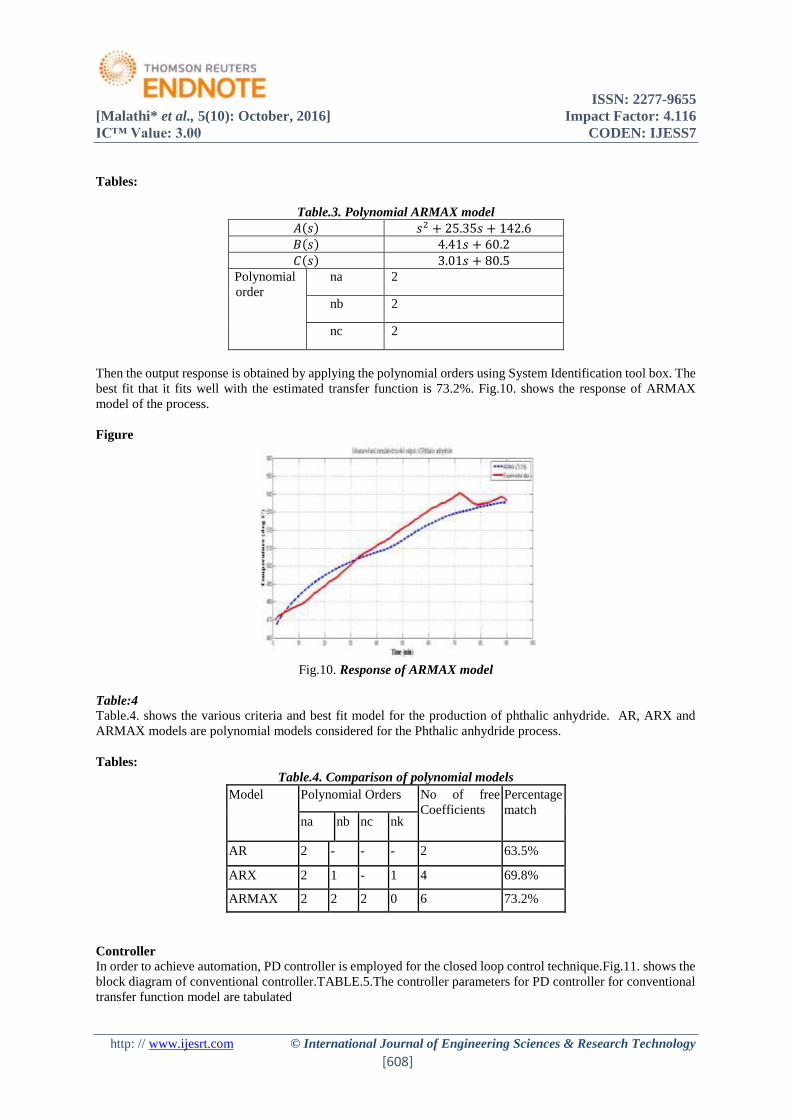
ARMAX model

ARX model identification is done by creating the iddata object. Then the model order specification is provided.

Then by specifying initial conditions ARX model transfer function is obtained along with the polynomial order.

Fig.9. shows the procedure to obtain ARMAX model for the process. TABLE.3. tabulates the polynomial

equations of the ARMAX model.

Figure

Fig.9. procedure to identify ARMAX model



Options for ARMAX model is specified

Search method has to specified

Specifying no of iterations

Transfer function obtained


ISSN: 2277-9655




[608]

Tables:

Table.3. Polynomial ARMAX model

𝐴(𝑠) 𝑠2 + 25.35𝑠 + 142.6

𝐵(𝑠) 4.41𝑠 + 60.2

𝐶(𝑠) 3.01𝑠 + 80.5

Polynomial

order

na 2

nb 2

nc 2

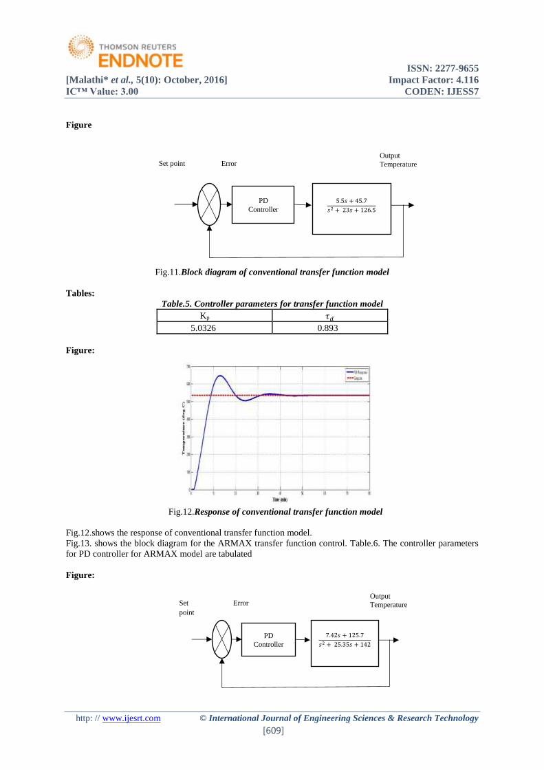
Then the output response is obtained by applying the polynomial orders using System Identification tool box. The

best fit that it fits well with the estimated transfer function is 73.2%. Fig.10. shows the response of ARMAX

model of the process.

Figure

Fig.10. Response of ARMAX model

Table:4

Table.4. shows the various criteria and best fit model for the production of phthalic anhydride. AR, ARX and

ARMAX models are polynomial models considered for the Phthalic anhydride process.

Tables:

Table.4. Comparison of polynomial models

Model Polynomial Orders No of free

Coefficients

Percentage

match na nb nc nk

AR 2 - - - 2 63.5%

ARX 2 1 - 1 4 69.8%

ARMAX 2 2 2 0 6 73.2%

Controller

In order to achieve automation, PD controller is employed for the closed loop control technique.Fig.11. shows the

block diagram of conventional controller.TABLE.5.The controller parameters for PD controller for conventional

transfer function model are tabulated


ISSN: 2277-9655




[609]

Figure

Fig.11.Block diagram of conventional transfer function model

Tables:

Table.5. Controller parameters for transfer function model

Kp 𝜏𝑑

5.0326 0.893

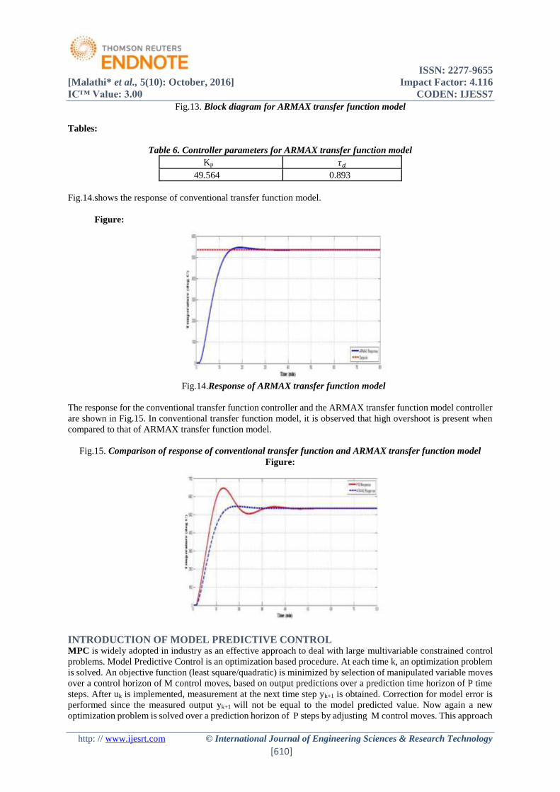
Figure:

Fig.12.Response of conventional transfer function model

Fig.12.shows the response of conventional transfer function model.

Fig.13. shows the block diagram for the ARMAX transfer function control. Table.6. The controller parameters

for PD controller for ARMAX model are tabulated

Figure:

PD

Controller

5.5𝑠 + 45.7

𝑠2 + 23𝑠 + 126.5

Set point Error Output

Temperature

PD

Controller

7.42𝑠 + 125.7

𝑠2 + 25.35𝑠 + 142

Set

point

Error Output

Temperature


ISSN: 2277-9655




[610]

Fig.13. Block diagram for ARMAX transfer function model

Tables:

Table 6. Controller parameters for ARMAX transfer function model

Kp 𝜏𝑑

49.564 0.893

Fig.14.shows the response of conventional transfer function model.

Figure:

Fig.14.Response of ARMAX transfer function model

The response for the conventional transfer function controller and the ARMAX transfer function model controller

are shown in Fig.15. In conventional transfer function model, it is observed that high overshoot is present when

compared to that of ARMAX transfer function model.

Fig.15. Comparison of response of conventional transfer function and ARMAX transfer function model

Figure:

INTRODUCTION OF MODEL PREDICTIVE CONTROL MPC is widely adopted in industry as an effective approach to deal with large multivariable constrained control

problems. Model Predictive Control is an optimization based procedure. At each time k, an optimization problem

is solved. An objective function (least square/quadratic) is minimized by selection of manipulated variable moves

over a control horizon of M control moves, based on output predictions over a prediction time horizon of P time

steps. After uk is implemented, measurement at the next time step yk+1 is obtained. Correction for model error is

performed since the measured output yk+1 will not be equal to the model predicted value. Now again a new

optimization problem is solved over a prediction horizon of P steps by adjusting M control moves. This approach


ISSN: 2277-9655




[611]

is called as receding control, this scheme introduces notion of feedback in the control law to compensate for

disturbances and modeling errors.Factors to be considered while implementing MPC are the type of objective

function used optimization, type of model used to predict the output, initialization of the model to predict future

output values, desired set-point trajectory, disturbance compensation and implementation of constraints.The basic

concept of MPC is to use a dynamic model to predict system behavior, and optimize the prediction to produce the

best decision — the control action at the current time. Based on the past and present values and future control

actions, the dynamic model predicts the future plant outputs. Optimizer calculates the control actions based on the

constraints presented as well as the objective function. Minimization of objective function is solving of the

optimization problem by adjusting control moves M which is subjected to modeling equations and input output

constraints.

In general for P prediction horizon & M control horizon,

Objective function is given as,

𝛗 = ∑ |𝐫𝐤+𝐢 − �̂�𝐤+𝐢| + 𝐰𝐏𝐢=𝟏 ∑ |∆𝐮𝐤+𝐢|

𝐌−𝟏𝐢=𝟏 and Optimization is min (φ).

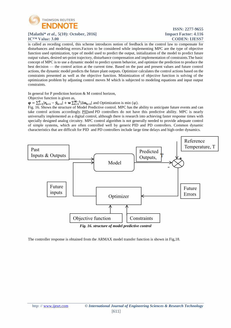
Fig. 16. Shows the structure of Model Predictive control. MPC has the ability to anticipate future events and can

take control actions accordingly. PIDand PD controllers do not have this predictive ability. MPC is nearly

universally implemented as a digital control, although there is research into achieving faster response times with

specially designed analog circuitry. MPC control algorithm is not generally needed to provide adequate control

of simple systems, which are often controlled well by generic PID and PD controllers. Common dynamic

characteristics that are difficult for PID and PD controllers include large time delays and high-order dynamics.

Fig. 16. structure of model predictive control

The controller response is obtained from the ARMAX model transfer function is shown in Fig,18.

Model

Optimizer

Future

inputs

Past

Inputs & Outputs

Future

Errors

Predicted

Outputs,

Reference

Temperature, T

+

-

Objective function Constraints


https://en.wikipedia.org/wiki/PID_controller

ISSN: 2277-9655




[612]

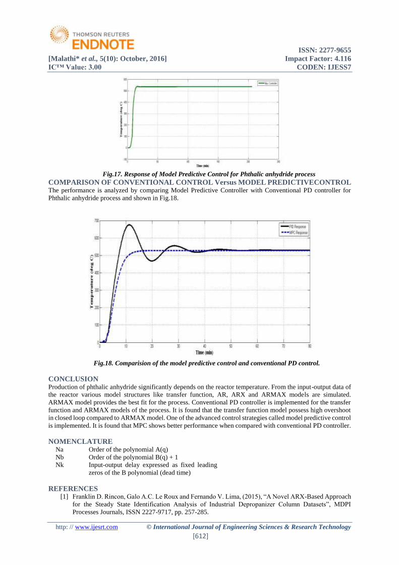
Fig.17. Response of Model Predictive Control for Phthalic anhydride process

COMPARISON OF CONVENTIONAL CONTROL Versus MODEL PREDICTIVECONTROL The performance is analyzed by comparing Model Predictive Controller with Conventional PD controller for

Phthalic anhydride process and shown in Fig.18.

Fig.18. Comparision of the model predictive control and conventional PD control.

CONCLUSION Production of phthalic anhydride significantly depends on the reactor temperature. From the input-output data of

the reactor various model structures like transfer function, AR, ARX and ARMAX models are simulated.

ARMAX model provides the best fit for the process. Conventional PD controller is implemented for the transfer

function and ARMAX models of the process. It is found that the transfer function model possess high overshoot

in closed loop compared to ARMAX model. One of the advanced control strategies called model predictive control

is implemented. It is found that MPC shows better performance when compared with conventional PD controller.

NOMENCLATURE Na Order of the polynomial A(q)

Nb Order of the polynomial B(q) + 1

Nk Input-output delay expressed as fixed leading

zeros of the B polynomial (dead time)

REFERENCES [1] Franklin D. Rincon, Galo A.C. Le Roux and Fernando V. Lima, (2015), “A Novel ARX-Based Approach

for the Steady State Identification Analysis of Industrial Depropanizer Column Datasets”, MDPI

Processes Journals, ISSN 2227-9717, pp. 257-285.


ISSN: 2277-9655




[613]

[2] Bhuvaneswari N S, Praveen R, Divya R, (2014), “System Identification and Modeling for Interacting

and Non-Interacting Tank Systems using Intelligent Techniques”, International Journal of Information

Sciences and Techniques, pp. 23-35.

[3] Muhammad Junaid Rabbani, Kashan Hussain, Asim-ur-Rehman khan, Abdullah Ali, (2013), “Model

Identification and Validation for a Heating System using MATLAB System Identification Toolbox”,

International Journal on Material Science and Engineering, ISSN 1757-8991, pp. 218-227.

[4] M. Shyamalagowri and R. Rajeswari, (2013), “Modeling and Simulation of Non-Linear Process Control

Reactor – Continuous Stirred Tank Reactor ”, International Journal of Advances in Engineering and

Technology, ISSN 22311963, pp. 1813-1818.

[5] Zahra’a F. Zuhwar, (2012), “The Control of Non Isothermal CSTR using Differential Controller

Strategies”, Iraqi Journal “.

[6] Nader Jamali Soufi Amlashi, Amin Shahsavari, Alireza Vahidifar, Mehrzad Nasirian, (2013), “Nonlinear

System Identification of Laboratory Heat Exchanger using Artificial Neural Network model”,

International Journal of Electrical and Computer Engineering, ISSN 2088-8708, pp. 118-128.

[7] George Stephanopoulos, (2006), ‘Chemical Process Control’, Prentice Hall India.

[8] Wayne B. Bequette, (2004), ‘Process Control: Design and Simulation’, Prince Hall of India.

[9] K. Krishnawamy, (2006), ‘Process Control’, New Age International Publishers.

[10] Thorsten Boger and Monica Menegola, “Monolithic Catalysts with High Thermal Conductivity for

Improved Operation and Economics in the Production of Phthalic Anhydride”, International journal of

Ind. Eng. Chem. Res., Vol 44, 2005, Pages 30-40

[11] G. Contillo, (2002), ‘Nonlinear Dynamics and Control in Process Engineering – Recent Advances’,

Springer-Verlag Italia, Milan.

[12] Lenart Ljung, (2000), ‘System Identification’, PTR Prince Hall Information and System Science.

[13] T.Ishikawa,Y.Natori “Modelling and optimisation of an industrial batch process for the production of

dioctyl phthalate”, International journal Computers and Chemical Engineering, Vol 21, 20 May 1997,

Pages S1239-S1244

[14] V.Nikolov, D.Klissurski & A.Anastasov, “Phthalic Anhydride from o-Xylene Catalysis: Science and

Engineering”, International journal of Catalysis Reviews, Vol 33, 1991, Pages 319-374

[15] http.mathworks.com/examples/sysid.

[16] http://www.mathworks.com/matlabcentral/answers/47212-how-to-make - transfer-function-if-you-

know-input-output-data.


Documents

LINEAR IDENTIFICATION AND CONTROL OF REACTOR FOR PHTHALIC ... /Archive-2016/October-2016/73.pdf · LINEAR IDENTIFICATION AND CONTROL OF REACTOR FOR PHTHALIC ANHYDRIDE PRODUCTION PROCESS