Embed Size (px)
Citation preview

LIMITS AND DERIVATIVESLIMITS AND DERIVATIVES
2
The problem of finding the tangent line
to a curve and the problem of finding
the velocity of an object both involve finding
the same type of limit—as we saw in
Section 2.1. This special type of limit is called a derivative.
LIMITS AND DERIVATIVES
2.7Derivatives and Rates
of Change
LIMITS AND DERIVATIVES
In this section, we will see that: the derivative can be interpreted as a rate
of change in any of the sciences or engineering.
If a curve C has equation y = f(x) and we want
to find the tangent line to C at the point
P(a,f(a)), then we consider a nearby point
Q(x,f(x)), where , and compute the slope
of the secant line PQ:
x a≠
( ) ( )PQ
f x f am
x a
−=
−
TANGENTS
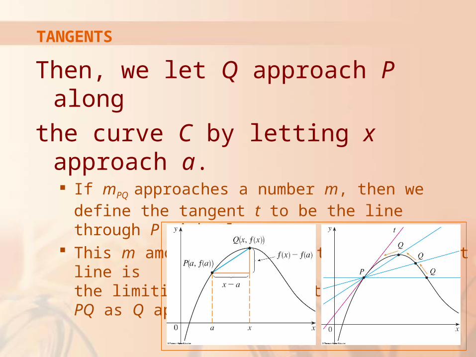
Then, we let Q approach P along
the curve C by letting x approach a. If mPQ approaches a number m, then we define the
tangent t to be the line through P with slope m. This m amounts to saying that the tangent line is
the limiting position of the secant line PQ as Q approaches P.
TANGENTS
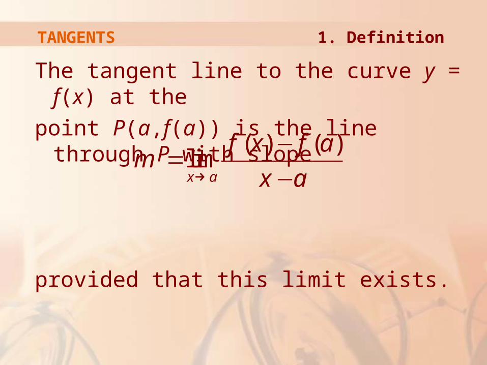
The tangent line to the curve y = f(x) at the
point P(a,f(a)) is the line through P with slope
provided that this limit exists.
( ) ( )limx a
f x f am
x a→
−=
−
TANGENTS 1. Definition

In our first example, we confirm
the guess we made in Example 1
in Section 2.1.
TANGENTS
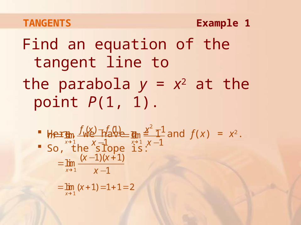
Find an equation of the tangent line to
the parabola y = x2 at the point P(1, 1).
Here, we have a = 1 and f(x) = x2. So, the slope is:
2
1 1
( ) (1) 1lim lim
1 1x x
f x f xm
x x→ →
− −= =
− −
1
( 1)( 1)lim
1x
x x
x→
− +=
−
1lim( 1) 1 1 2x
x→
= + = + =
TANGENTS Example 1
Using the point-slope form of the
equation of a line, we find that an
equation of the tangent line at (1, 1) is:
y - 1 = 2(x - 1) or y = 2x - 1
TANGENTS Example 1
We sometimes refer to the slope of the
tangent line to a curve at a point as the
slope of the curve at the point. The idea is that, if we zoom in far enough toward the
point, the curve looks almost like a straight line.
TANGENTS
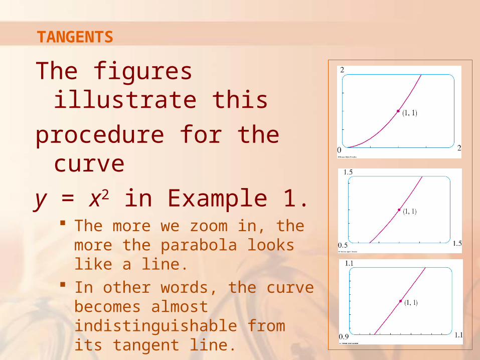
The figures illustrate this
procedure for the curve
y = x2 in Example 1. The more we zoom in, the more
the parabola looks like a line. In other words, the curve becomes
almost indistinguishable from its tangent line.
TANGENTS
There is another expression for the slope of a
tangent line that is sometimes easier to use.
If h = x - a, then x = a + h and so the slope
of the secant line PQ is:
( ) ( )PQ
f a h f am
h
+ −=
TANGENTS
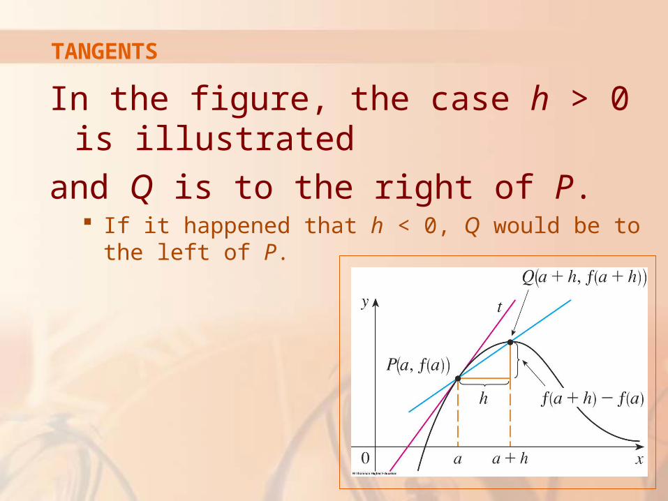
In the figure, the case h > 0 is illustrated
and Q is to the right of P. If it happened that h < 0, Q would be to the left of P.
TANGENTS
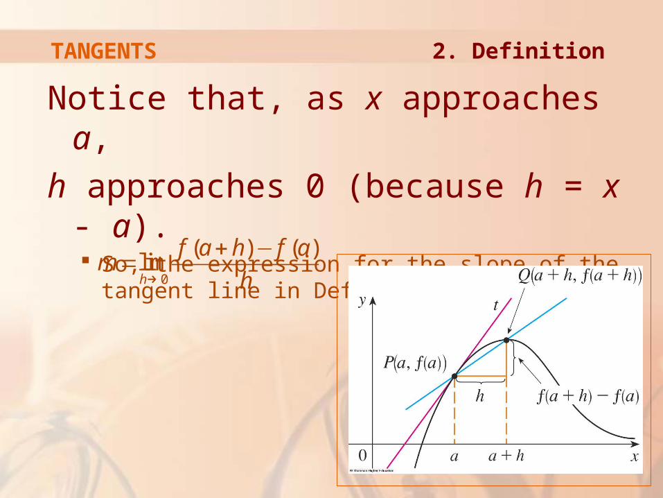
Notice that, as x approaches a,
h approaches 0 (because h = x - a). So, the expression for the slope of the tangent line in
Definition 1 becomes:
0
( ) ( )limh
f a h f am
h→
+ −=
TANGENTS 2. Definition
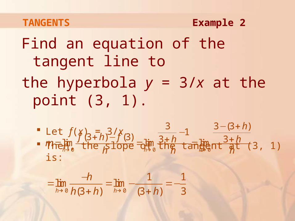
Find an equation of the tangent line to
the hyperbola y = 3/x at the point (3, 1).
Let f(x) = 3/x Then, the slope of the tangent at (3, 1) is:
0 0 0
3 3 (3 )1(3 ) (3) 3 3lim lim lim
h h h
hf h f h hm
h h h→ → →
− +−+ − + += = =
0 0
1 1lim lim
(3 ) (3 ) 3h h
h
h h h→ →
−= = − =−
+ +
TANGENTS Example 2
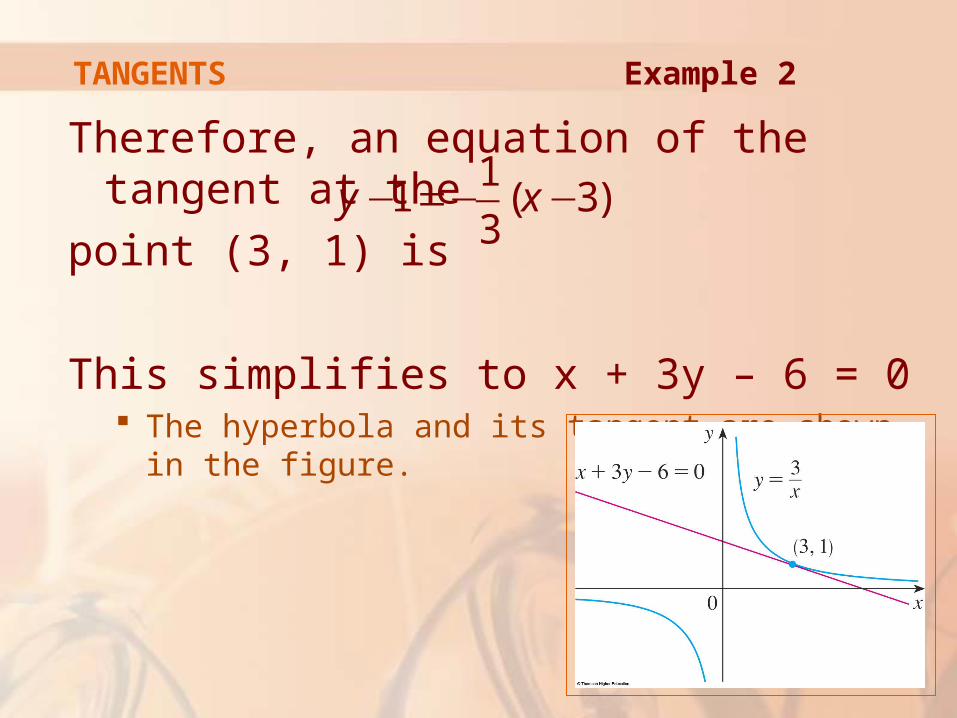
Therefore, an equation of the tangent at the
point (3, 1) is
This simplifies to x + 3y – 6 = 0 The hyperbola and its tangent are shown in the figure.
11 ( 3)
3y x− =− −
TANGENTS Example 2
In Section 2.1, we investigated the motion
of a ball dropped from the CN Tower and
defined its velocity to be the limiting value
of average velocities over
shorter and shorter time
periods.
VELOCITIES
In general, suppose an object moves
along a straight line according to an
equation of motion s = f(t) S is the displacement (directed distance) of the object
from the origin at time t. The function f that describes the motion is called
the position function of the object.
VELOCITIES
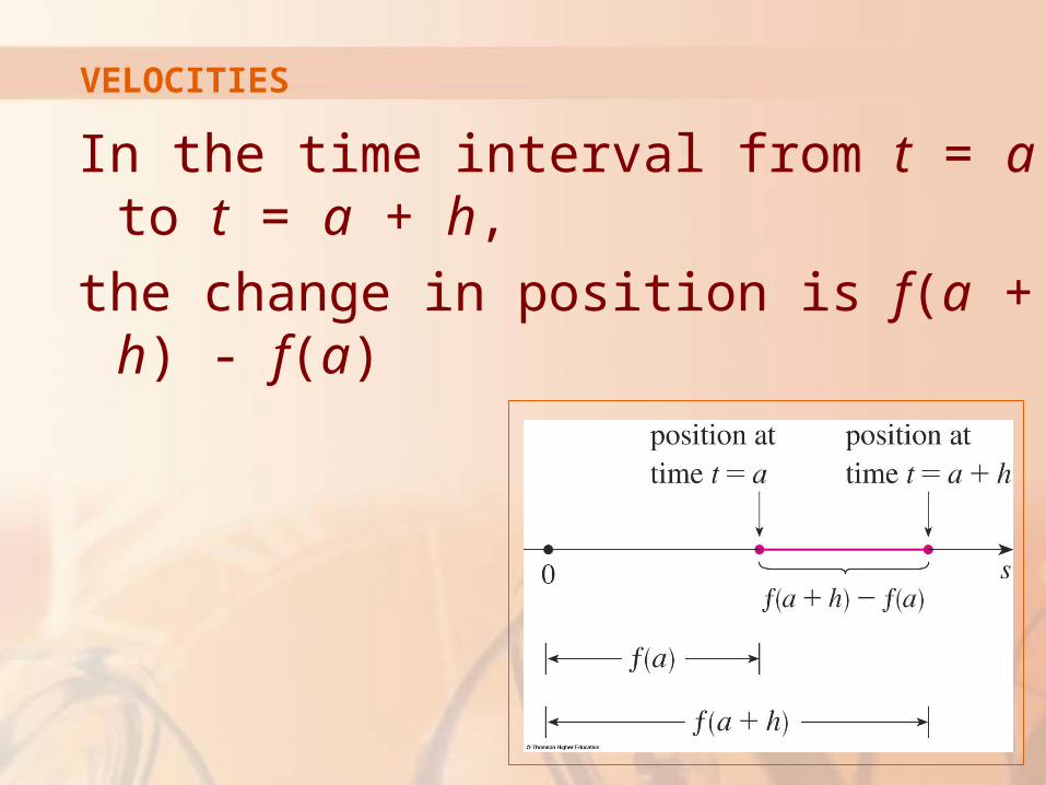
In the time interval from t = a to t = a + h,
the change in position is f(a + h) - f(a)
VELOCITIES
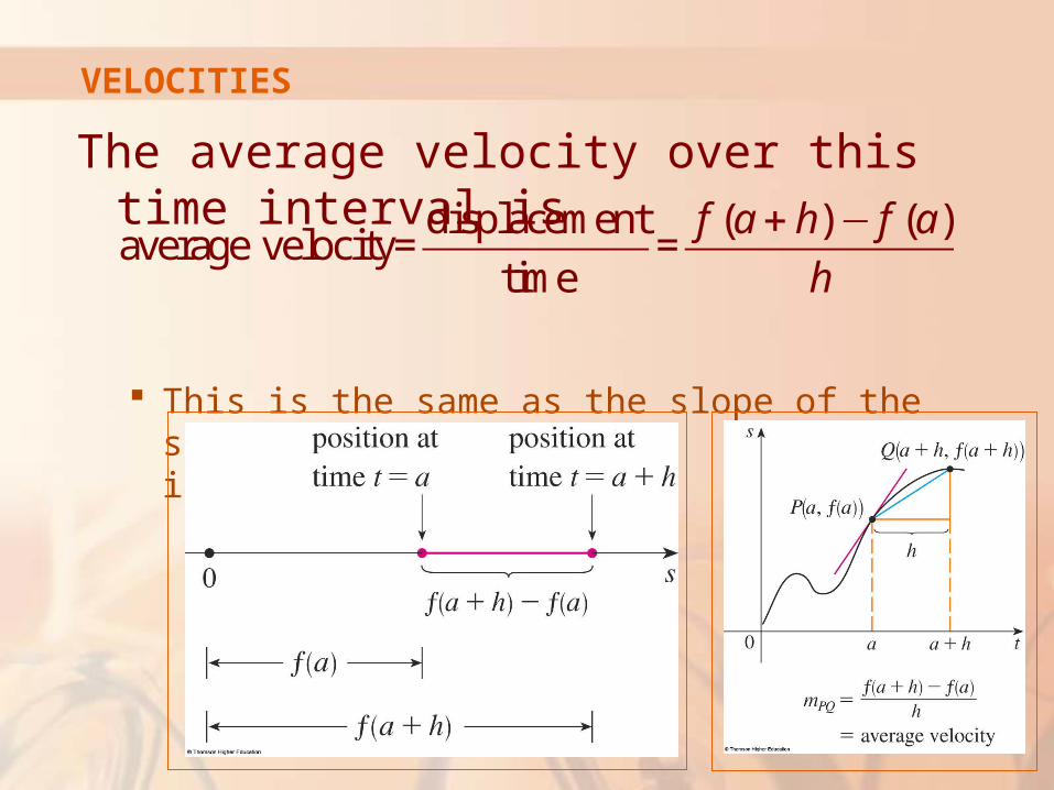
The average velocity over this time interval is
This is the same as the slope of the secant line PQ in the second figure.
displacement ( ) ( )average velocity= =
time
f a h f a
h
+ −
VELOCITIES
Now, suppose we compute the
average velocities over shorter and
shorter time intervals [a, a + h]. In other words, we let h approach 0.
VELOCITIES
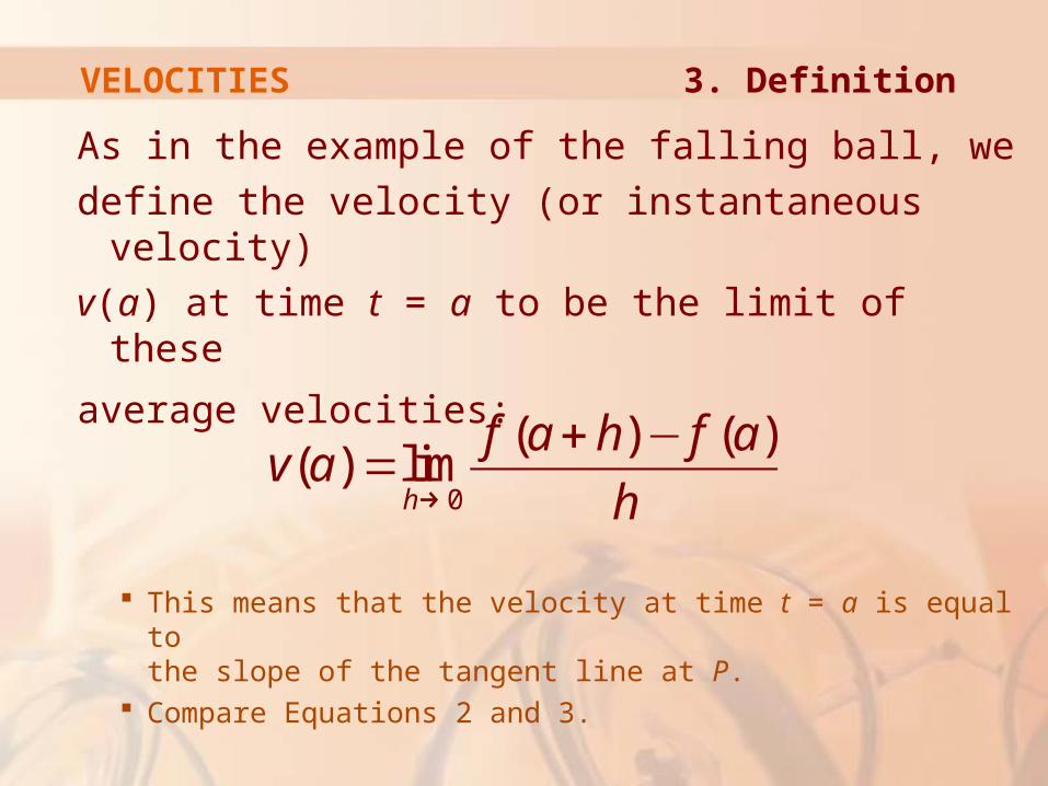
As in the example of the falling ball, we
define the velocity (or instantaneous velocity)
v(a) at time t = a to be the limit of these
average velocities:
This means that the velocity at time t = a is equal to the slope of the tangent line at P.
Compare Equations 2 and 3.
0
( ) ( )( ) lim
h
f a h f av a
h→
+ −=
VELOCITIES 3. Definition
Now that we know how to compute
limits, let’s reconsider the problem
of the falling ball.
VELOCITIES
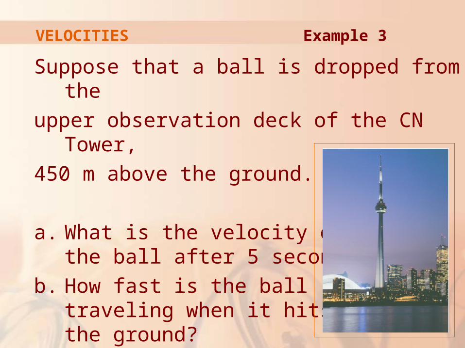
Suppose that a ball is dropped from the
upper observation deck of the CN Tower,
450 m above the ground.
a. What is the velocity of the ball after 5 seconds?
b. How fast is the ball traveling when it hits the ground?
VELOCITIES Example 3
We will need to find the velocity both
when t = 5 and when the ball hits the
ground. So, it’s efficient to start by finding the velocity at
a general time t = a
VELOCITIES Example 3
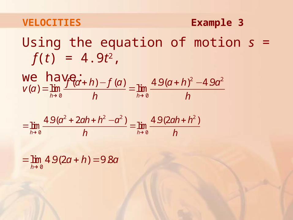
Using the equation of motion s = f(t) = 4.9t2,
we have:2 2
0 0
( ) ( ) 4.9( ) 4.9( ) lim lim
h h
f a h f a a h av a
h h→ →
+ − + −= =
2 2 2 2
0 0
4.9( 2 ) 4.9(2 )lim limh h
a ah h a ah h
h h→ →
+ + − += =
0lim4.9(2 ) 9.8h
a h a→
= + =
VELOCITIES Example 3
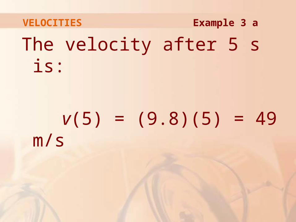
The velocity after 5 s is:
v(5) = (9.8)(5) = 49 m/s
VELOCITIES Example 3 a
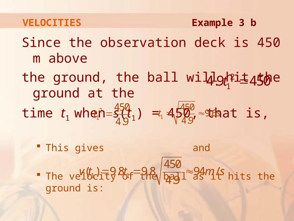
Since the observation deck is 450 m above
the ground, the ball will hit the ground at the
time t1 when s(t1) = 450, that is,
This gives and
The velocity of the ball as it hits the ground is:
214.9 450t =
21
450
4.9t = 1
4509.6
4.9t s= ≈
1 1
450( ) 9.8 9.8 94 /
4.9v t t m s= = ≈
VELOCITIES Example 3 b
We have seen that the same type of limit
arises in finding the slope of a tangent
line (Equation 2) or the velocity of an
object (Equation 3).
DERIVATIVES
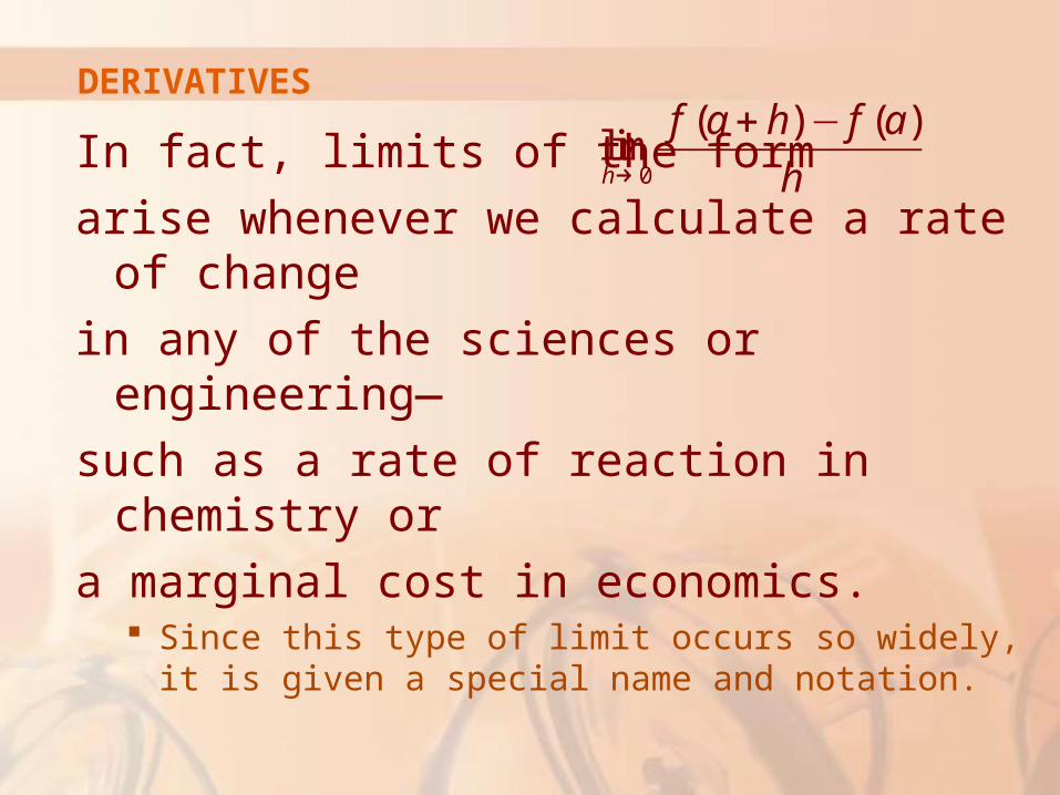
In fact, limits of the form
arise whenever we calculate a rate of change
in any of the sciences or engineering—
such as a rate of reaction in chemistry or
a marginal cost in economics. Since this type of limit occurs so widely, it is given a
special name and notation.
DERIVATIVES
0
( ) ( )limh
f a h f a
h→
+ −
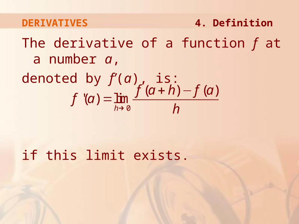
The derivative of a function f at a number a,
denoted by f’(a), is:
if this limit exists.
0
( ) ( )'( ) lim
h
f a h f af a
h→
+ −=
DERIVATIVES 4. Definition
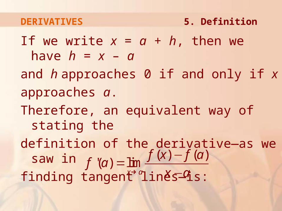
If we write x = a + h, then we have h = x – a
and h approaches 0 if and only if x
approaches a.
Therefore, an equivalent way of stating the
definition of the derivative—as we saw in
finding tangent lines—is:
( ) ( )'( ) lim
x a
f x f af a
x a→
−=
−
DERIVATIVES 5. Definition
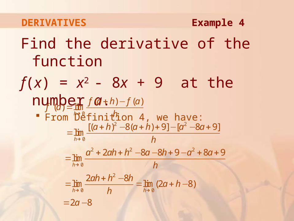
Find the derivative of the function
f(x) = x2 - 8x + 9 at the number a. From Definition 4, we have:
0
2 2
0
2 2 2
0
2
0 0
( ) ( )'( ) lim
[( ) 8( ) 9] [ 8 9]lim
2 8 8 9 8 9lim
2 8lim lim(2 8)
2 8
h
h
h
h h
f a h f af a
h
a h a h a a
h
a ah h a h a a
h
ah h ha h
ha
→
→
→
→ →
+ −=
+ − + + − − +=
+ + − − + − + +=
+ −= = + −
= −
DERIVATIVES Example 4
We defined the tangent line to the curve
y = f(x) at the point P(a,f(a)) to be the line that
passes through P and has slope m given by
Equation 1 or 2.
Since, by Definition 4, this is the same as the
derivative f’(a), we can now say the following. The tangent line to y = f(x) at (a,f(a)) is the line
through (a,f(a)) whose slope is equal to f’(a), the derivative of f at a.
DERIVATIVES
If we use the point-slope form of the equation
of a line, we can write an equation of the
tangent line to the curve y = f(x) at the point
(a,f(a)):
y - f(a) = f’(a)(x - a)
DERIVATIVES
Find an equation of the tangent line
to the parabola y = x2 - 8x + 9 at
the point (3, -6).
From Example 4, we know that the derivative of f(x) = x2 - 8x + 9 at the number a is f’(a) = 2a - 8
Therefore, the slope of the tangent line at (3, -6) is f’(3) = 2(3) – 8 = -2.
DERIVATIVES Example 5
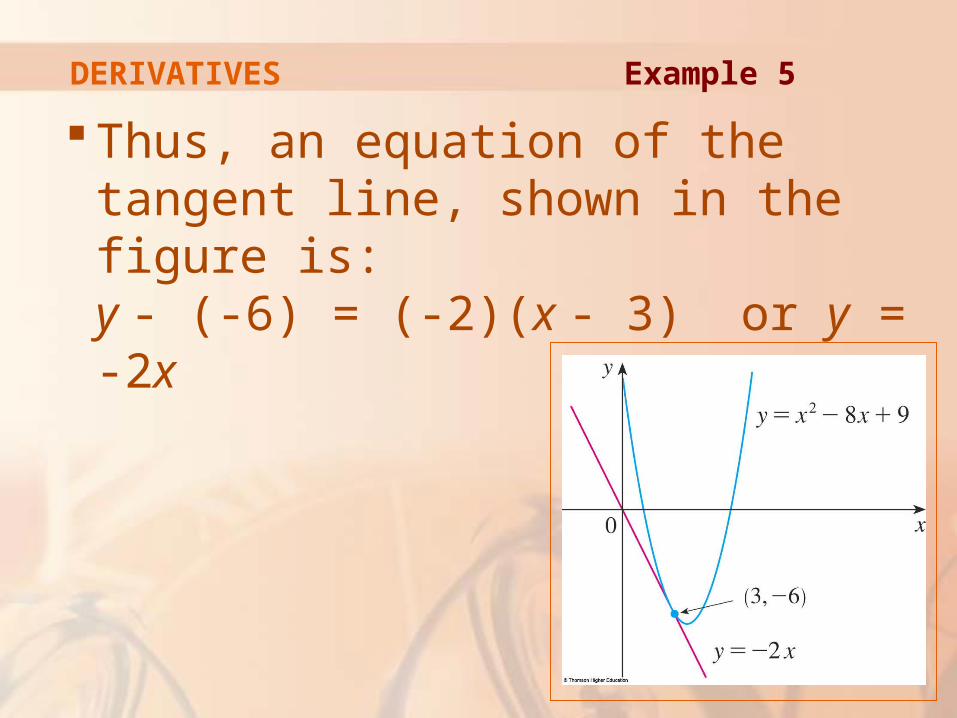
Thus, an equation of the tangent line, shown in the figure is: y - (-6) = (-2)(x - 3) or y = -2x
DERIVATIVES Example 5
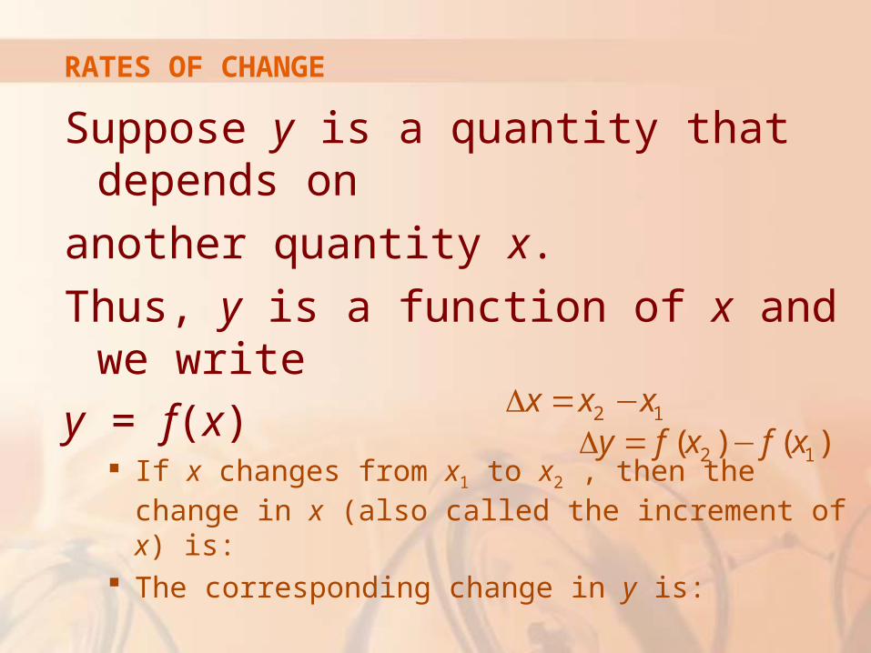
Suppose y is a quantity that depends on
another quantity x.
Thus, y is a function of x and we write
y = f(x) If x changes from x1 to x2 , then the change in x (also
called the increment of x) is: The corresponding change in y is:
2 1x x xΔ = −2 1( ) ( )y f x f xΔ = −
RATES OF CHANGE
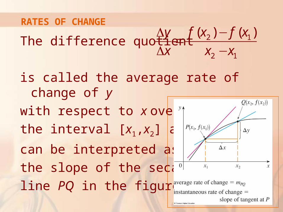
The difference quotient
is called the average rate of change of y
with respect to x over
the interval [x1,x2] and
can be interpreted as
the slope of the secant
line PQ in the figure.
2 1
2 1
( ) ( )f x f xy
x x x
−Δ=
Δ −
RATES OF CHANGE
By analogy with velocity, we consider
the average rate of change over smaller and
smaller intervals by letting x2 approach x1
and, therefore, letting approach 0. The limit of these average rates of change is called
the (instantaneous) rate of change of y with respect to x at x = x1.
xΔ
RATES OF CHANGE
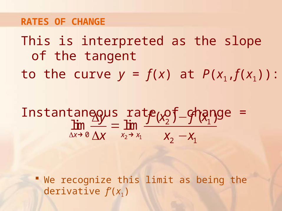
This is interpreted as the slope of the tangent
to the curve y = f(x) at P(x1,f(x1)):
Instantaneous rate of change =
We recognize this limit as being the derivative f’(x1)
2 1
2 1
02 1
( ) ( )lim limx x x
f x f xy
x x xΔ → →
−Δ=
Δ −
RATES OF CHANGE
We know that one interpretation of the
derivative f’(a) is as the slope of the tangent
line to the curve y = f(x) when x = a.
We now have a second interpretation. The derivative f’(a) is the instantaneous rate of change
of y = f(x) with respect to x when x = a.
RATES OF CHANGE
The connection with the first interpretation
is that, if we sketch the curve y = f(x), then
the instantaneous rate of change is the slope
of the tangent to this curve at the point
where x = a.
RATES OF CHANGE
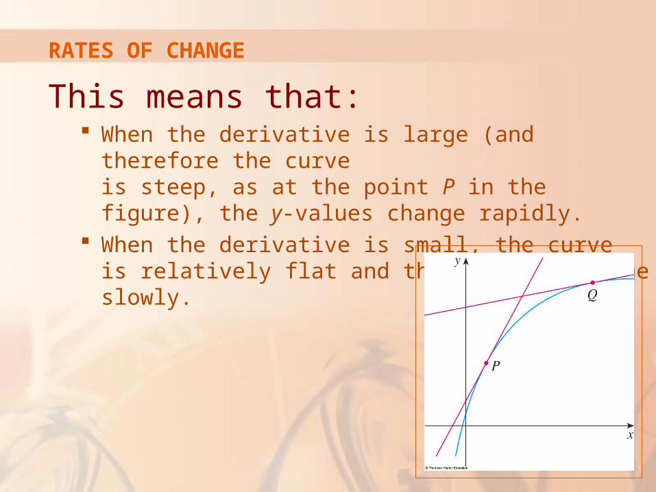
This means that: When the derivative is large (and therefore the curve
is steep, as at the point P in the figure), the y-values change rapidly.
When the derivative is small, the curve is relatively flat and the y-values change slowly.
RATES OF CHANGE
In particular, if s = f(t) is the position function
of a particle that moves along a straight line,
then f’(a) is the rate of change of the
displacement s with respect to the time t. In other words, f’(a) is the velocity of the particle
at time t = a. The speed of the particle is the absolute value of
the velocity, that is, |f’(a)|.
RATES OF CHANGE

In the next example, we discuss
the meaning of the derivative of
a function that is defined verbally.
RATES OF CHANGE
A manufacturer produces bolts of a fabric
with a fixed width.
The cost of producing x yards of this fabric
is C = f(x) dollars.a. What is the meaning of the derivative f’(x)?
What are its units?
b. In practical terms, what does it mean to say that f’(1,000) = 9?
c. Which do you think is greater, f’(50) or f’(500)? What about f’(5,000)?
RATES OF CHANGE Example 6
The derivative f’(x) is the instantaneous
rate of change of C with respect to x.
That is, f’(x) means the rate of change
of the production cost with respect to
the number of yards produced. Economists call this rate of change the marginal cost.
RATES OF CHANGE Example 6 a
As
the units for f’(x) are the same as
the units for the difference quotient . Since is measured in dollars and in yards,
it follows that the units for f’(x) are dollars per yard.
0'( ) lim
x
Cf x
xΔ →
Δ=
Δ
Cx
ΔΔ
CΔ xΔ
RATES OF CHANGE Example 6 a
The statement that f’(1,000) = 9 means that,
after 1,000 yards of fabric have been
manufactured, the rate at which the
production cost is increasing is $9/yard. When x =1,000, C is increasing 9 times as fast as x.
RATES OF CHANGE Example 6 b
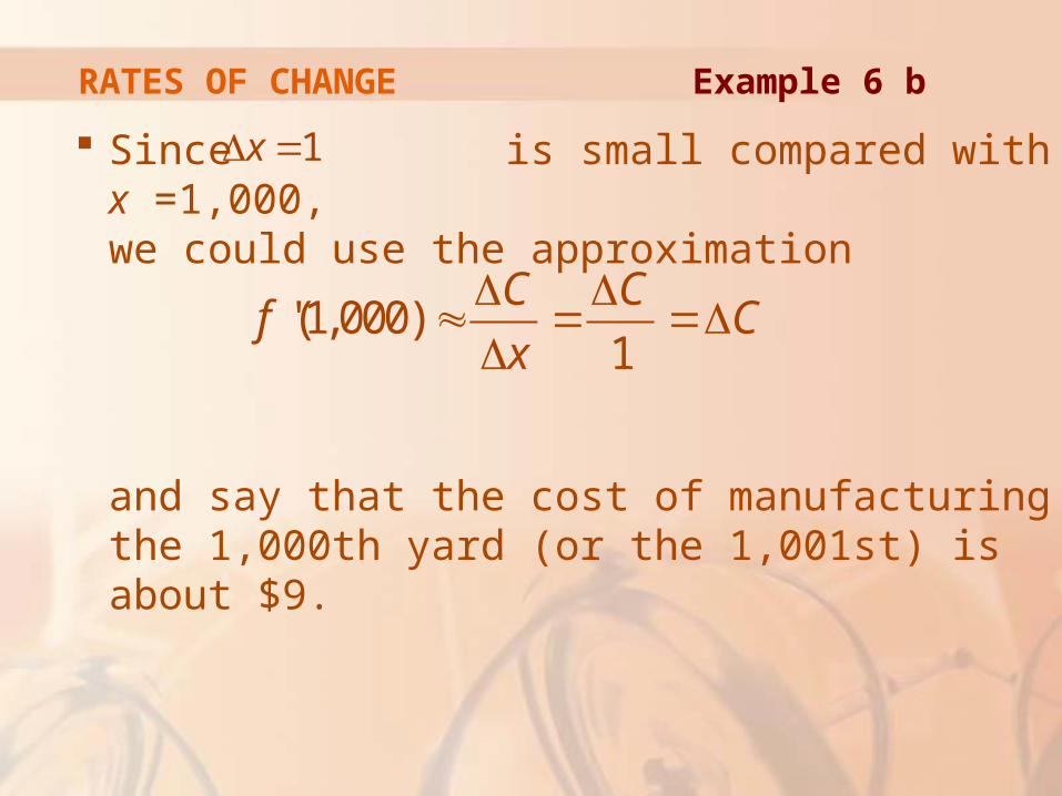
Since is small compared with x =1,000, we could use the approximation
and say that the cost of manufacturing the 1,000th yard (or the 1,001st) is about $9.
'(1,000)1
C Cf C
x
Δ Δ≈ = =Δ
Δ
1xΔ =
RATES OF CHANGE Example 6 b
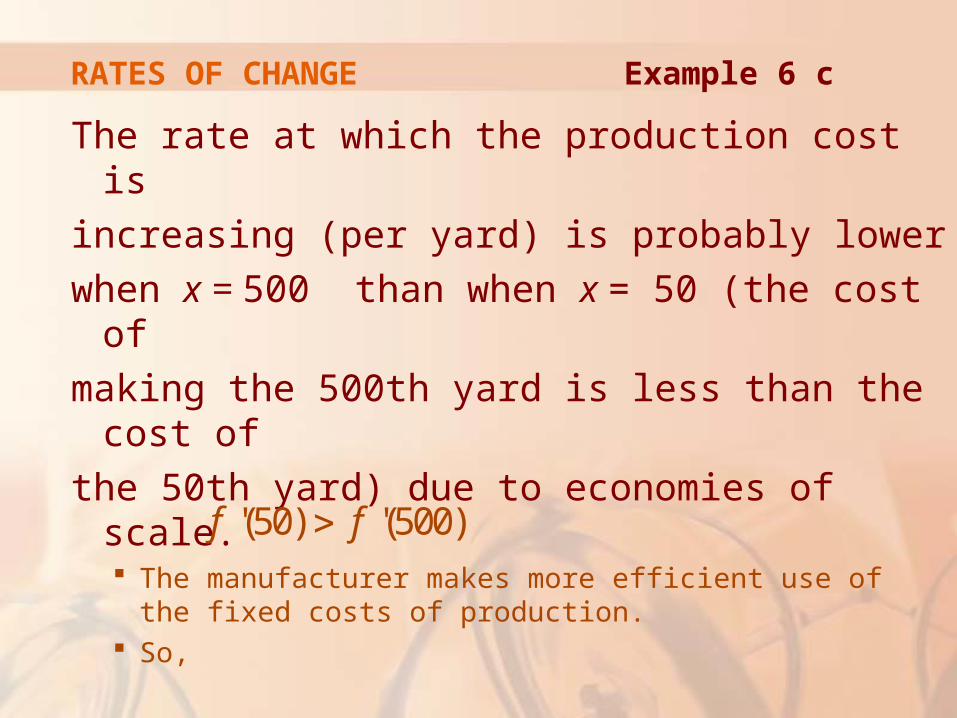
The rate at which the production cost is
increasing (per yard) is probably lower
when x = 500 than when x = 50 (the cost of
making the 500th yard is less than the cost of
the 50th yard) due to economies of scale. The manufacturer makes more efficient use of
the fixed costs of production. So, '(50) '(500)f f>
RATES OF CHANGE Example 6 c
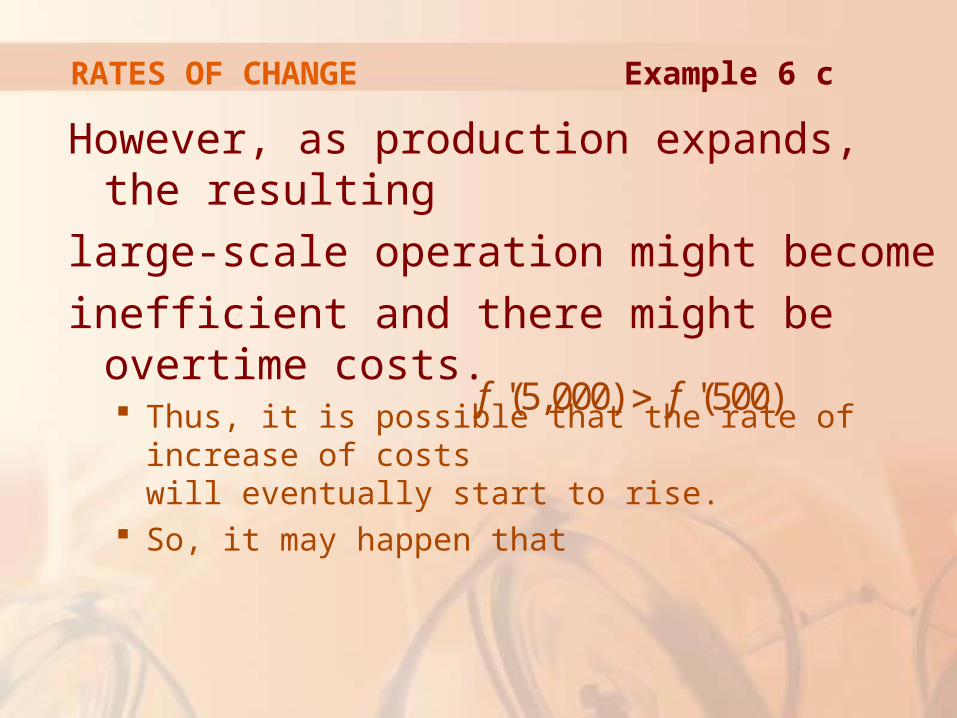
However, as production expands, the resulting
large-scale operation might become
inefficient and there might be overtime costs. Thus, it is possible that the rate of increase of costs
will eventually start to rise. So, it may happen that '(5,000) '(500)f f>
RATES OF CHANGE Example 6 c
In the following example, we estimate
the rate of change of the national debt
with respect to time. Here, the function is defined not by a formula but by
a table of values.
RATES OF CHANGE
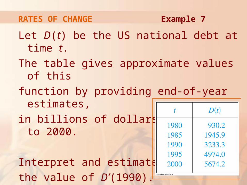
Let D(t) be the US national debt at time t.
The table gives approximate values of this
function by providing end-of-year estimates,
in billions of dollars, from 1980 to 2000.
Interpret and estimate
the value of D’(1990).
RATES OF CHANGE Example 7
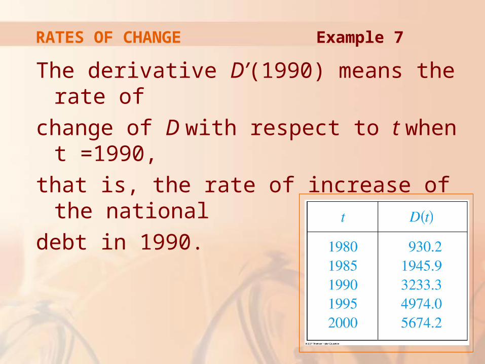
The derivative D’(1990) means the rate of
change of D with respect to t when t =1990,
that is, the rate of increase of the national
debt in 1990.
RATES OF CHANGE Example 7
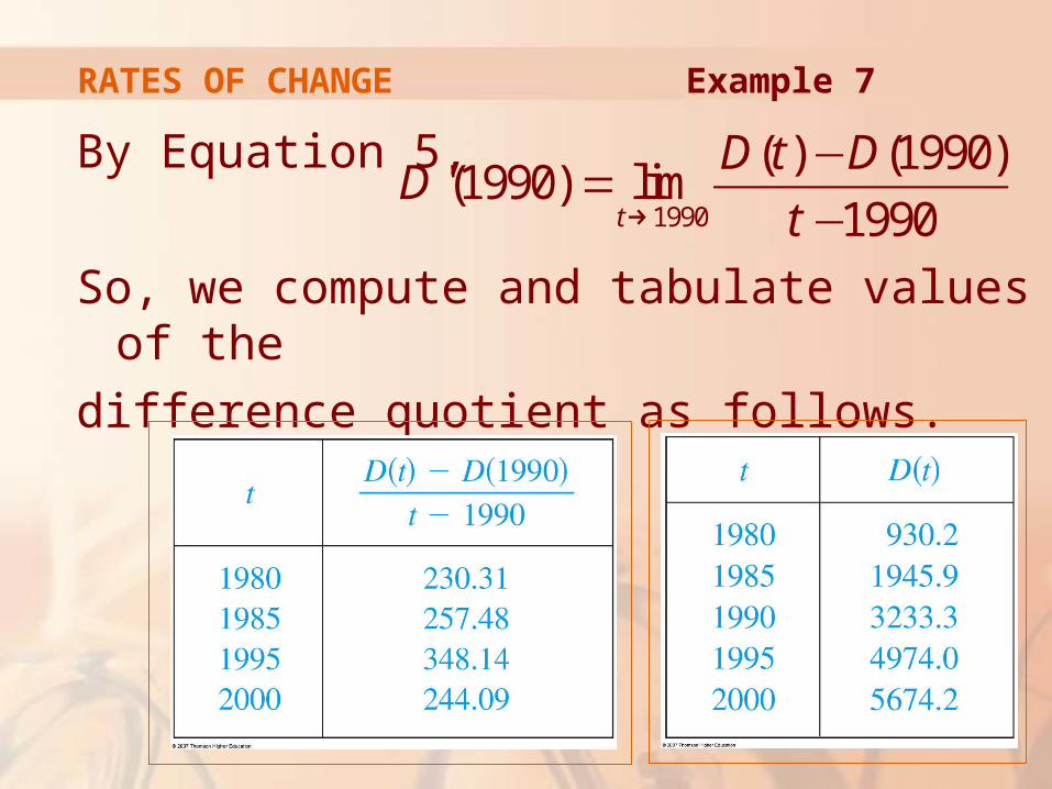
By Equation 5,
So, we compute and tabulate values of the
difference quotient as follows.
RATES OF CHANGE Example 7
1990
( ) (1990)'(1990) lim
1990t
D t DD
t→
−=
−
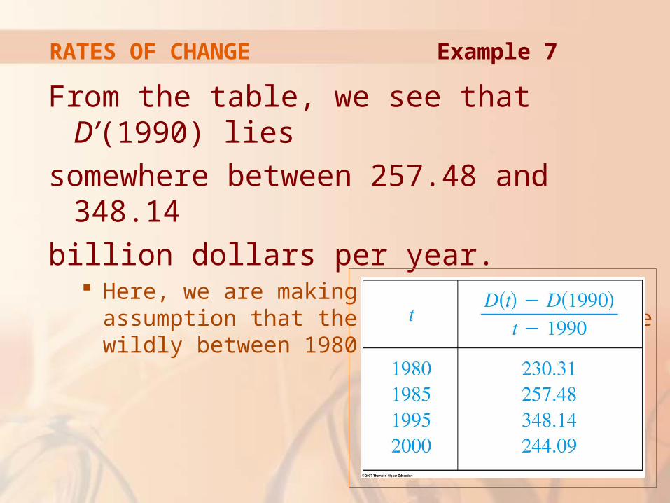
From the table, we see that D’(1990) lies
somewhere between 257.48 and 348.14
billion dollars per year. Here, we are making the reasonable assumption that
the debt didn’t fluctuate wildly between 1980 and 2000.
RATES OF CHANGE Example 7
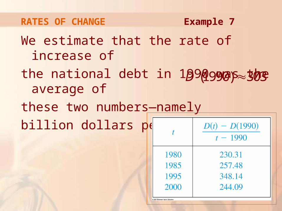
We estimate that the rate of increase of
the national debt in 1990 was the average of
these two numbers—namely
billion dollars per year.
'(1990) 303D ≈
RATES OF CHANGE Example 7

Another method would be to plot the
debt function and estimate the slope of
the tangent line when t = 1990.
RATES OF CHANGE Example 7
In Examples 3, 6, and 7, we saw three
specific examples of rates of change: The velocity of an object is the rate of change of
displacement with respect to time. The marginal cost is the rate of change of production
cost with respect to the number of items produced. The rate of change of the debt with respect to time is
of interest in economics.
RATES OF CHANGE
Here is a small sample of other rates
of change: In physics, the rate of change of work with respect to
time is called power. Chemists who study a chemical reaction are interested
in the rate of change in the concentration of a reactant with respect to time (called the rate of reaction).
A biologist is interested in the rate of change of the population of a colony of bacteria with respect to time.
RATES OF CHANGE
In fact, the computation of rates of
change is important in all the natural
sciences, in engineering, and even in
the social sciences.
RATES OF CHANGE
All these rates of change are derivatives
and can therefore be interpreted as
slopes of tangents. This gives added significance to the solution of
the tangent problem.
RATES OF CHANGE
Whenever we solve a problem involving
tangent lines, we are not just solving
a problem in geometry. We are also implicitly solving a great variety of problems
involving rates of change in science and engineering.
RATES OF CHANGE