Thermal Pressurization of Pore Fluid

During Earthquake Slip

Liliana Hromadova

2009

Thermal Pressurization of Pore Fluid

During Earthquake Slip

MASTER’S THESIS

Liliana Hromadova

Comenius University

Faculty of Mathematics, Physics and Informatics

Department of Astronomy, Physics of the Earth, and Meteorology

4.1.1 Physics

Supervisor: Prof. RNDr. Peter Moczo, DrSc.

Bratislava 2009

Acknowledgements

The author thanks her supervisor, Professor Peter Moczo, for his guidance, help and

support. His understanding and broad-mindedness are also highly appreciated. The

author also thanks Docent Peter Guba for a very useful discussion.

II

Abstract

Liliana Hromadova

Thermal Pressurization of Pore Fluid During Earthquake Slip

Comenius University

Faculty of Mathematics, Physics and Informatics

Department of Astronomy, Physics of the Earth, and Meteorology

Supervisor: Prof. RNDr. Peter Moczo, DrSc.

Bratislava 2009

93 pages

The presented thesis is intended as a detailed analysis of a candidate dynamic fault

weakening mechanism called thermal pressurization of pore fluid, based on the theory

of thermoporoelasticity and on the latest geological, laboratory, and theoretical field

results.

The thesis starts with a summary of the most important dynamic fault weaken-

ing mechanisms, possibly playing a significant role during large tectonic earthquakes,

i.e., the thermal pressurization of pore fluid, the flash heating of microscopic asperity

contacts, the melting, and the silica gel formation. In the following chapter, an intro-

duction to the theory of thermoporoelasticity is presented, emphasized on a detailed

establishment of the theory of linear poroelasticity, and containing a generalization to a

thermoporoelastic case. It is the most extensive chapter of the thesis, since the thermal

pressurization of pore fluid process can be treated as a thermoporoelastic problem. In

the next, final chapter, a modified physical model of the thermal pressurization of pore

fluid process is proposed. The chapter starts with a summary of latest geological, labo-

ratory, and theoretical findings regarding the thermal pressurization process, resulting

in model properties, constraints and assumptions, and in a set of appropriate values of

model parameters. Then the geometry, material properties, physical mechanism, and

governing equations of the model are presented. One of the governing equations, which

describes the pore fluid pressure variations, differs from the commonly used one - it

contains two additional non-linear terms. The performed dimensional analysis suggests

III

that at least one of the two non-linear terms cannot be omitted in the governing equa-

tion.

Keywords: tectonic earthquakes, dynamic fault weakening, frictional heating, ther-

mal pressurization of pore fluid, thermoporoelasticity.

IV

Abstrakt

Liliana Hromadova

Teplom indukovane zvysenie tlaku tekutiny v poroch

pocas sklzu pri tektonickom zemetrasenı

Univerzita Komenskeho v Bratislave

Fakulta matematiky, fyziky a informatiky

Katedra astronomie, fyziky Zeme a meteorologie

Skolitel: Prof. RNDr. Peter Moczo, DrSc.

Bratislava 2009

93 stran

Predkladana diplomova praca je zamerana na detailnu analyzu fyzikalneho procesu

teplom indukovaneho zvysenia tlaku tekutiny v poroch pocas sklzu pri tektonickom

zemetrasenı. Uvedeny proces je dolezitym kandidatom na vysvetlenie dynamickeho

oslabovania tektonickeho zlomu pocas zemetrasenia. Analyza procesu je zalozena na

teorii termoporoelasticity a na najnovsıch vysledkoch geologickeho, laboratorneho a

teoretickeho vyskumu relevantneho pre skumany proces.

Praca zacına sumarizaciou a strucnym popisom najdolezitejsıch potencialnych me-

chanizmov na vysvetlenie dynamickeho oslabovania zlomu pocas zemetrasenia. Su to

nasledovne styri mechanizmy: teplom indukovane zvysenie tlaku tekutiny v poroch,

nahly ohrev a oslabenie mikroskopickych kontaktov, natavenie horniny, formovanie

kremiciteho gelu. Druha kapitola je koncipovana ako uvod do teorie termoporoelastici-

ty s dorazom kladenym na podrobne vybudovanie teorie linearnej poroelasticity, ktora

je nasledne zovseobecnena na termoporoelasticky prıpad. Ide o najobsiahlejsiu kapi-

tolu prace. Podrobnost a rozsiahlost vykladu je motivovana tym, ze skumany proces

teplom indukovaneho zvysenia tlaku tekutiny v poroch mozno klasifikovat ako ter-

moporoelasticky problem. V zaverecnej kapitole je navrhnuty modifikovany fyzikalny

model skumaneho procesu. Kapitola zacına sumarizaciou najnovsıch geologickych, la-

boratornych a teoretickych vysledkov tykajucich sa procesu. Nasledne je navrhnuty

V

subor hodnot modelovych parametrov. Kapitola pokracuje prezentovanım geometrie,

materialovych vlastnostı, mechanizmu a riadiacich rovnıc modelu. Riadiace rovnice su

odvodene z rovnıc termoporoelasticity aplikovanım vlastnostı fyzikalneho modelu. Ria-

diace rovnice su nakoniec transformovane do bezrozmerneho tvaru a jednotlive cleny su

kvantifikovane na zaklade hodnot modelovych parametrov. Rozmerova analyza ukazuje,

ze nelinearne cleny v rovnici pre variacie teploty mozno zanedbat a jej linearizovany

tvar je teda postacujuci na popis skumaneho procesu. Tento vysledok je v zhode s

literaturou. Avsak analogicka rozmerova analyza aplikovana na druhu rovnicu, t.j.

rovnicu pre variacie tlaku tekutiny v poroch, ukazuje, ze minimalne jeden nelinearny

clen v rovnici nemozno zanedbat. Preto sa domnievame, ze na korektny popis procesu

teplom indukovaneho zvysenia tlaku tekutiny v poroch nemozno pouzit linearizovany

tvar rovnice, ktory je bezne pouzıvany v dostupnych fyzikalnych modeloch procesu.

Klucove slova: tektonicke zemetrasenia, dynamicke oslabovanie zlomu, ohrev trenım,

zvysenie tlaku tekutiny v poroch, termoporoelasticita.

VI

Foreword

Understanding the mechanisms responsible for the dynamic weakening of tectonic

faults during earthquakes is still a great challenge in geophysics, although the earth-

quake source dynamics, probably pioneered with the spring-and-box model of Burridge

and Knopoff (1967), has been studied for more than 40 years. At the present level of

knowledge, four different dynamic fault weakening mechanisms may possibly act du-

ring large tectonic earthquakes: thermal pressurization of pore fluid, flash heating of

microscopic asperity contacts, melting, and silica gel formation. The first two of them

seem to be the primary weakening mechanisms, probably acting in combination, as

supported by strong experimental and theoretical indications.

Owing to these facts, we decided to focus on the process of thermal pressurization

of pore fluid in the presented thesis. The primary future goal is to include the thermal

pressurization process in the existing numerical model on rupture propagation, deve-

loped by the team of numerical modeling of seismic wave propagation and earthquake

motion in the Division of the Physics of the Earth under supervision of Professor Peter

Moczo.

The analysis is based both on the theory of thermoporoelasticity and on the pub-

lished articles on the thermal pressurization process. Mainly the books of Charlez

(1991), Detournay and Cheng (1993), Wang, H. (2000), Coussy (2004), and the arti-

cles of Biot (1941), Lachenbruch (1980), Palciauskas and Domenico (1982), Mase and

Smith (1985), McTigue (1986), Andrews (2002), Bizzarri and Cocco (2006a), Rempel

(2006), Rempel and Rice (2006), Rice (2006) are followed in the thesis.

The text is divided into three chapters - starting with an introductory text on the

dynamic weakening mechanisms of tectonic earthquakes, followed by a detailed intro-

duction in the theory of thermoporoelasticity, and ending with a physical model of the

investigated process. The given text structure was motivated by the fact that a detailed

development and presentation of the physical model of the thermal pressurization of

pore fluid process starting from the theory of thermoporoelasticity is lacking in the

literature.

VII

Our effort results in presentation of an introductory text on the theory of thermoporoelasticity, concise overview of the latest geological, laboratory, and theoretical findings regar-

ding the thermal pressurization of pore fluid process, proposal of a modified physical model of the process, derivation of the governing equations of the process.

One of the derived governing equations differs from the commonly used one. Whereas

the commonly used equation is linear, we propose a non-linear equation. According to

the presented dimensional analysis, at least one non-linear term cannot be omitted in

the governing equation. Therefore, we think that the generally used linearized equation

is not appropriate for the thermal pressurization of pore fluid process, and the non-

linear one proposed here should be used instead.

VIII

Contents

1 Introduction . . . . . . . . . . . . . . . . . . . . . . . . . . . . . . . . . . . . . . . . . . . . . . . . . . . . . . . 1

2 Introduction to Linear Poroelasticity

with Extension to Thermoporoelasticity . . . . . . . . . . . . . . . . . . . . . . . . . . . . . . . . . 7

2.1 Overview . . . . . . . . . . . . . . . . . . . . . . . . . . . . . . . . . . . . . . . . . . . . . . . . . . . . . . . 7

2.1.1 Theory of Linear Poroelasticity . . . . . . . . . . . . . . . . . . . . . . . . . . . . . . . 7

2.1.2 Theory of Linear Thermoporoelasticity . . . . . . . . . . . . . . . . . . . . . . . . 9

2.2 Variables . . . . . . . . . . . . . . . . . . . . . . . . . . . . . . . . . . . . . . . . . . . . . . . . . . . . . . . 10

2.2.1 Strain . . . . . . . . . . . . . . . . . . . . . . . . . . . . . . . . . . . . . . . . . . . . . . . . . . . . . 11

2.2.2 Variation of Fluid Content . . . . . . . . . . . . . . . . . . . . . . . . . . . . . . . . . . . 12

2.2.3 Pore Fluid Pressure . . . . . . . . . . . . . . . . . . . . . . . . . . . . . . . . . . . . . . . . . 15

2.2.4 Stress . . . . . . . . . . . . . . . . . . . . . . . . . . . . . . . . . . . . . . . . . . . . . . . . . . . . . 16

2.2.5 Variables of Linear Thermoporoelasticity . . . . . . . . . . . . . . . . . . . . . . . 18

2.3 Constitutive Equations . . . . . . . . . . . . . . . . . . . . . . . . . . . . . . . . . . . . . . . . . . . 19

2.3.1 Effective Stress Concept . . . . . . . . . . . . . . . . . . . . . . . . . . . . . . . . . . . . . 22

2.3.2 Constitutive Equations of Linear Thermoporoelasticity . . . . . . . . . . . 24

2.4 Poroelastic Parameters . . . . . . . . . . . . . . . . . . . . . . . . . . . . . . . . . . . . . . . . . . . 25

2.4.1 Lame’s Parameters . . . . . . . . . . . . . . . . . . . . . . . . . . . . . . . . . . . . . . . . . . 25

2.4.2 Compressibilities . . . . . . . . . . . . . . . . . . . . . . . . . . . . . . . . . . . . . . . . . . . . 27

2.4.3 Poisson’s Ratio . . . . . . . . . . . . . . . . . . . . . . . . . . . . . . . . . . . . . . . . . . . . . 31

2.4.4 Storage Coefficients . . . . . . . . . . . . . . . . . . . . . . . . . . . . . . . . . . . . . . . . . 32

2.4.5 Pore Fluid Pressure Buildup Coefficients . . . . . . . . . . . . . . . . . . . . . . . 33

2.4.6 Hydraulic Diffusivity . . . . . . . . . . . . . . . . . . . . . . . . . . . . . . . . . . . . . . . . 35

2.4.7 Parameters of Linear Thermoporoelasticity . . . . . . . . . . . . . . . . . . . . . 36

2.5 Governing Equations . . . . . . . . . . . . . . . . . . . . . . . . . . . . . . . . . . . . . . . . . . . . . 38

2.5.1 Force Balance Equations . . . . . . . . . . . . . . . . . . . . . . . . . . . . . . . . . . . . . 39

2.5.2 Fluid Diffusivity Equation . . . . . . . . . . . . . . . . . . . . . . . . . . . . . . . . . . . 41

2.5.3 Governing Equations of Linear Thermoporoelasticity . . . . . . . . . . . . 48

3 Thermal Pressurization of Pore Fluid Process

During Earthquake Slip . . . . . . . . . . . . . . . . . . . . . . . . . . . . . . . . . . . . . . . . . . . 54

3.1 Overview . . . . . . . . . . . . . . . . . . . . . . . . . . . . . . . . . . . . . . . . . . . . . . . . . . . . . . . 54

3.2 Physical Model . . . . . . . . . . . . . . . . . . . . . . . . . . . . . . . . . . . . . . . . . . . . . . . . . . 55

3.2.1 Geological, Laboratory, and Theoretical Findings . . . . . . . . . . . . . . . . 55

3.2.2 Values of Model Parameters . . . . . . . . . . . . . . . . . . . . . . . . . . . . . . . . . . 61

IX

3.2.3 Geometry and Material Properties . . . . . . . . . . . . . . . . . . . . . . . . . . . . 62

3.2.4 Physical Mechanism . . . . . . . . . . . . . . . . . . . . . . . . . . . . . . . . . . . . . . . . . 63

3.2.5 Governing Equations . . . . . . . . . . . . . . . . . . . . . . . . . . . . . . . . . . . . . . . . 67

3.2.6 Primary Shortcomings of the Presented Model . . . . . . . . . . . . . . . . . . 78

3.3 Main Points of Controversy and Open Questions . . . . . . . . . . . . . . . . . . . . . 81

4 Conclusions . . . . . . . . . . . . . . . . . . . . . . . . . . . . . . . . . . . . . . . . . . . . . . . . . . . . . . . 82

References . . . . . . . . . . . . . . . . . . . . . . . . . . . . . . . . . . . . . . . . . . . . . . . . . . . . . . . . . . . . 84

X

Notation index

(the SI physical unit is given in square braces, a reference to the definition is given in round braces)

Ap net area of pores per unit bulk volume [m2 ]

A0 surface area of the bulk volume [m2 ]

B Skempton coefficient (2.89)

G shear modulus [Pa]

G∗ shear modulus of elastic medium [Pa]

H inverse of poroelastic expansion coefficient [Pa]

J Jacobian of transformation (2.14)

K drained bulk modulus [Pa] (2.51)

K rate of kinetic energy [J s−1 ]

Kf pore fluid bulk modulus [Pa] (2.71)

Kp drained pore bulk modulus [Pa]

Ks solid bulk modulus [Pa] (2.65)

K′

s unjacketed bulk modulus [Pa] (2.59)

K′′

s unjacketed pore modulus [Pa] (2.60)

Ku undrained bulk modulus [Pa]

M Biot modulus [Pa] (2.83)

Pc confining pressure [Pa] (2.40)

Pd differential pressure [Pa] (Terzaghi’s effective pressure) (2.39)

Pe effective pressure [Pa] (2.42)

P′

e Terzaghi’s effective pressure (differential pressure) [Pa] (2.39)

δ Q heat supply to the system [J ]

Qs heat source [J m−3 s−1 ]

Re Reynolds number (2.130)

S entropy [J K−1 ] (2.34)

Sa uniaxial specific storage coefficient [Pa−1 ] (2.84)

Sγ unjacketed specific storage coefficient (coefficient of fluid content) [Pa−1 ] (2.88)

Sε constrained specific storage coefficient [Pa−1 ] (2.82)

Sσ unconstrained specific storage coefficient [Pa−1 ] (2.79)

T temperature [K ] (2.34)

XI

∆U slip [m]

U rate of internal energy [J s−1 ]

Vb bulk volume [m3 ]

Vf pore fluid volume [m3 ]

Vp volume of pores [m3 ]

Vs solid volume [m3 ]

∆Vs slip rate [m s−1 ]

We rate of work of external forces [J s−1 ]

c Kozeny constant

cb specific heat capacity of the bulk material [J kg−1 K−1 ]

ce effective volumetric heat capacity [J m−3 K−1 ] (2.113)

cf specific heat capacity of the pore fluid [J kg−1 K−1 ]

cs specific heat capacity of the solid material [J kg−1 K−1 ]

f coefficient of friction

~f body force per unit bulk volume [N m−3 ]

gm specific free pore fluid enthalpy [J kg−1 ]

hm specific pore fluid enthalpy [J kg−1 ] (2.167)

k (intrinsic) permeability [m2 ] (2.102)

kf pore fluid thermal conductivity [J s−1 m−1 K−1 ]

ks solid thermal conductivity [J s−1 m−1 K−1 ]

kth effective thermal conductivity [J s−1 m−1 K−1 ] (2.115)

l characteristic pore size [m]

mf fluid mass content [kg m−3 ] (2.7)

n Lagrangian porosity (2.8)

~n0 unit normal vector

p pore fluid pressure [Pa]

q Darcy’s velocity [m s−1 ] (2.127)

qth heat flux [J s−1 m−2 ] (2.163)

s0 entropy per unit bulk volume [J K−1 m−3 ]

s0f entropy of the pore fluid per unit fluid volume [J K−1 m−3 ]

XII

sm specific pore fluid entropy [J K−1 kg−1 ]

t time [s]

ttot total slip duration at a point [s]

u matrix displacement [m]

uf pore fluid displacement [m]

um specific pore fluid internal energy [J kg−1 ]

uv bulk internal energy per unit volume [J m−3 ]

v seepage velocity [m s−1 ] (2.128)

vf pore fluid velocity [m s−1 ]

vs solid velocity [m s−1 ]

wc fault core half-width [m]

ws principal slipping zone half-width [m]

~x position vector [m]

α Biot-Willis coefficient (effective stress coefficient) (2.57)

αb drained bulk thermal expansivity [K−1 ] (2.103)

αf pore fluid thermal expansivity [K−1 ] (2.104)

αhy hydraulic diffusivity [m2 s−1 ] (2.99)

αm fluid mass content thermal expansivity [K−1 ] (2.110)

αp pore volume thermal expansivity [K−1 ] (2.107)

αs solid thermal expansivity [K−1 ] (2.105)

αth thermal diffusivity [m2 s−1 ] (2.114)

αu undrained bulk thermal expansivity [K−1 ] (2.111)

β effective stress coefficient for the pore volume (2.58)

βb drained bulk compressibility [Pa−1 ] (2.47)

βvb uniaxial bulk compressibility [Pa−1 ] (2.52)

βbp bulk volume expansion coefficient [Pa−1 ] (2.48)

βf pore fluid bulk compressibility [Pa−1 ] (2.70)

βpPcdrained pore compressibility [Pa−1 ] (2.49)

βpp pore volume expansion coefficient [Pa−1 ] (2.50)

βs solid bulk compressibility [Pa−1 ]

XIII

δ increment in the corresponding quantity

δij Dirac delta function

εij strain (2.1)

εkk bulk volumetric strain (2.2)

εfkk pore fluid volumetric strain (2.4)

εskk solid volumetric strain (2.5)

ζ variation of fluid content (2.6)

η poroelastic stress coefficient (2.86)

Θ non-dimensional temperature (3.28)

λ drained Lame’s first parameter [Pa]

λ∗ Lame’s first elastic parameter [Pa]

λu undrained Lame’s first parameter [Pa]

µ dynamic fluid viscosity [Pa s]

ν drained Poisson’s ratio (2.75)

νu undrained Poisson’s ratio (2.76)

ξ non-dimensional position (3.28)

Π non-dimensional pore fluid pressure (3.28)

Π′

non-dimensional Terzaghi’s effective pressure (3.29)

ρb bulk density [kg m−3 ]

ρf pore fluid density [kg m−3 ]

ρs solid density [kg m−3 ]

σ mean normal stress [Pa] (2.25)

σij (total) stress [Pa]

σ∗ij (total) stress in elastic medium [Pa] (2.45)

σij effective stress [Pa] (2.37)

σ′

ij Terzaghi’s effective stress [Pa] (2.38)

σfij pore fluid (macroscopic) partial stress [Pa] (2.30)

σsij solid (macroscopic) partial stress [Pa] (2.31)

σfij pore fluid microscopic stress [Pa] (2.27)

σsij solid microscopic stress [Pa]

σoct octahedral stress [Pa] (2.24)

XIV

τ non-dimensional time (3.28)

τ fij pore fluid viscous shear stress [Pa]

φ Eulerian porosity (2.9)

Φ dissipation of energy [J m−3 s−1 ] (2.172)

Φ1 intrinsic dissipation [J m−3 s−1 ] (2.173)

Φ2 thermohydraulic dissipation [J m−3 s−1 ] (2.174)

ψ0 volumetric free energy [J m−3 ] (2.170)

XV

List of Figures

Fig. 1: An illustration of the bulk material. . . . . . . . . . . . . . . . . . . . . . 8

Fig. 2: The principal slipping zone of the Punchbowl fault,

based on Chester et al. (2005). . . . . . . . . . . . . . . . . . . . . . . . . 58

Fig. 3: A schematic fault zone model. . . . . . . . . . . . . . . . . . . . . . . . . . 59

Fig. 4: Model geometry. . . . . . . . . . . . . . . . . . . . . . . . . . . . . . . . . . . 65

Fig. 5: A schematic illustration of the thermal pressurization

process mechanism. . . . . . . . . . . . . . . . . . . . . . . . . . . . . . . . . 66

List of Tables

Tab. 1: Values of model parameters. A: Geological, seismological

and observational parameters. . . . . . . . . . . . . . . . . . . . . . . . 63

Tab. 2: Values of model parameters. B: Laboratory

determined parameters. . . . . . . . . . . . . . . . . . . . . . . . . . . . 64

Tab. 3: Values of model parameters. B: Theoretically

determined parameters. . . . . . . . . . . . . . . . . . . . . . . . . . . . 65

XVI

1 Introduction

There are several different types of earthquakes: tectonic, volcanic, collapse, and in-

duced. In this thesis, only the tectonic earthquakes are treated. They are the most

common earthquakes (they represent about 90% of all earthquakes), and result from

regional or global tectonic processes.

Tectonic earthquakes. Tectonic earthquakes are natural phenomena accompanied

by a sudden release of mechanical energy accumulated in the Earth’s lithosphere. A

typical tectonic earthquake does not occur by a creation and propagation of a new

rupture in an unfaulted, intact rock. Instead, it occurs predominantly by a frictional

sliding along a pre-existing, already weakened zone of finite thickness separating two

blocks of the Earth’s lithosphere. Such zones are called fault zones, or simply, faults.

They are situated mainly at the boundaries between the Earth’s lithospheric plates

(the transform plate boundaries, to be specific), but some of the faults are also inside

the plates. However, the tectonic earthquake is not a purely frictional phenomenon -

the interfacial sliding is accompanied by a destruction of microscopic intermolecular

bonds which have been rebuilt during an interseismic period (i.e., the time period be-

tween two subsequent earthquakes on the fault). It means that a rupture has to be

re-created and propagated on the fault too, although having only a secondary role in

the earthquake mechanism (Scholz, 1998). The tectonic earthquake should be therefore

understood as a phenomenon comprising both the frictional sliding and the rupture

creation and propagation mechanisms. (For brevity, the term earthquake instead of

tectonic earthquake is hereafter used.)

Cause and mechanism of earthquakes. During the interseismic period, con-

siderable amounts of stresses and strains are being accumulated on the fault. It is a

consequence of global tectonic processes leading to a large-scale relative motion between

the adjacent lithospheric plates. At the same time, however, a part of the contact area

of the plates can be at rest due to the static friction. The shear stress is being accu-

mulated at a given point of the fault until it reaches the value of the material strength

1

at the point, given by the friction law and called frictional strength. “Should the shear

stress exceed the frictional strength at the point, a slip, i.e., a relative displacement of

the two fault faces occurs” (Moczo et al., 2007). The subsequent evolution of the shear

stress follows the friction law. It is a well established fact that the shear stress grad-

ually decreases with the increasing slip at the point during an earthquake. It implies

that the decrease has to be due to some dynamic weakening mechanisms. The exis-

tence of strong dynamic fault weakening mechanisms is also supported by the latest

friction experiments performed under coseismic slip-rates and nearly coseismic con-

fining stresses, which clearly imply that the fault strength under coseismic conditions

is much lower than that under conditions of lower slip rates and lower confining stresses.

Dynamic fault weakening mechanisms. Several mechanisms have been pro-

posed so far to explain the dynamic fault weakening behavior during earthquakes.

According to the latest theoretical results, and data from laboratory experiments and

in-situ geological measurements, the following mechanisms are the most possible can-

didates for explanation of the dynamic fault weakening behavior (Rice and Cocco,

2006): Thermal pressurization of pore fluid. Flash heating of microscopic asperity contacts. Melting. Silica gel formation.

The first three mechanisms listed above are of thermal nature. The latest field observa-

tions of mature, highly slipped faults (e.g., the San Andreas fault system in California,

or the Median Tectonic Line fault system in Japan) suggest that earthquake slips are

accommodated primarily within extremely thin slipping zones (≈ 1 mm). Given to it

the fact that slips on mature faults are relatively rapid, with a typical slip-rate of 1 ms−1

(Heaton, 1990), a considerable amount of frictional heat is assumed to be generated

on the fault during slip. Therefore, the primary weakening mechanisms are likely to be

thermal mechanisms induced by frictional heating (Fialko, 2004), i.e., heating due to

the interfacial sliding on the fault.

2

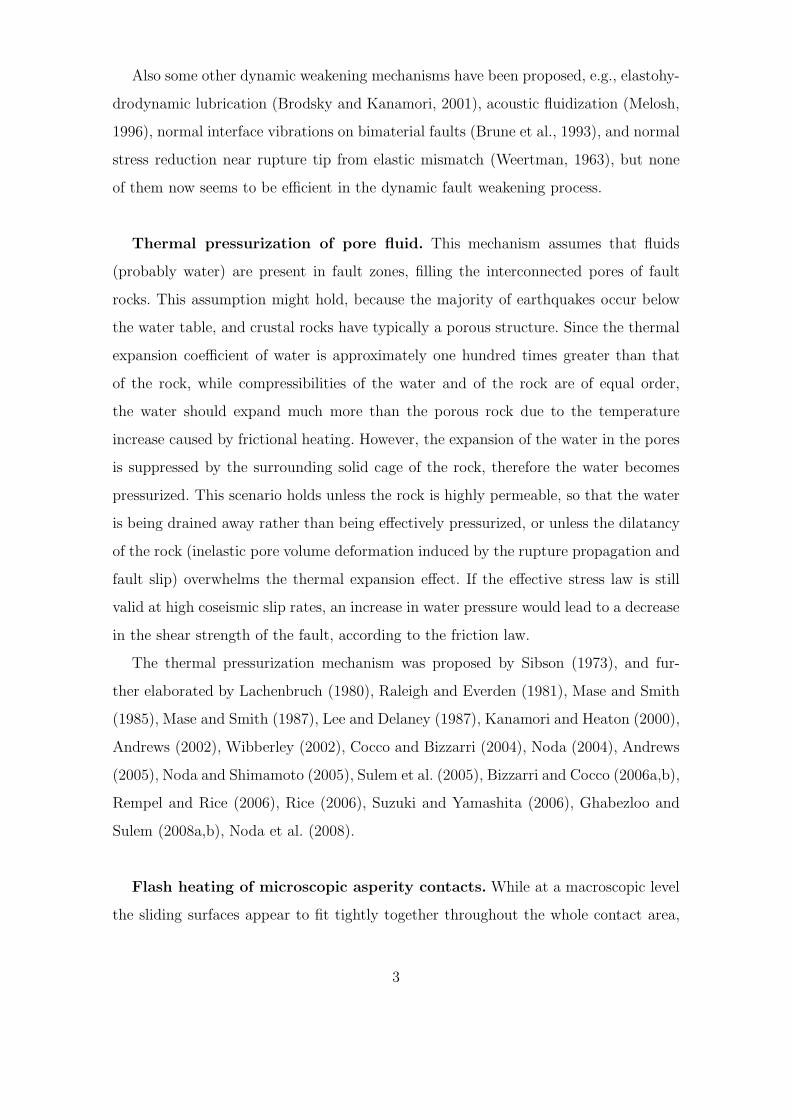
Also some other dynamic weakening mechanisms have been proposed, e.g., elastohy-

drodynamic lubrication (Brodsky and Kanamori, 2001), acoustic fluidization (Melosh,

1996), normal interface vibrations on bimaterial faults (Brune et al., 1993), and normal

stress reduction near rupture tip from elastic mismatch (Weertman, 1963), but none

of them now seems to be efficient in the dynamic fault weakening process.

Thermal pressurization of pore fluid. This mechanism assumes that fluids

(probably water) are present in fault zones, filling the interconnected pores of fault

rocks. This assumption might hold, because the majority of earthquakes occur below

the water table, and crustal rocks have typically a porous structure. Since the thermal

expansion coefficient of water is approximately one hundred times greater than that

of the rock, while compressibilities of the water and of the rock are of equal order,

the water should expand much more than the porous rock due to the temperature

increase caused by frictional heating. However, the expansion of the water in the pores

is suppressed by the surrounding solid cage of the rock, therefore the water becomes

pressurized. This scenario holds unless the rock is highly permeable, so that the water

is being drained away rather than being effectively pressurized, or unless the dilatancy

of the rock (inelastic pore volume deformation induced by the rupture propagation and

fault slip) overwhelms the thermal expansion effect. If the effective stress law is still

valid at high coseismic slip rates, an increase in water pressure would lead to a decrease

in the shear strength of the fault, according to the friction law.

The thermal pressurization mechanism was proposed by Sibson (1973), and fur-

ther elaborated by Lachenbruch (1980), Raleigh and Everden (1981), Mase and Smith

(1985), Mase and Smith (1987), Lee and Delaney (1987), Kanamori and Heaton (2000),

Andrews (2002), Wibberley (2002), Cocco and Bizzarri (2004), Noda (2004), Andrews

(2005), Noda and Shimamoto (2005), Sulem et al. (2005), Bizzarri and Cocco (2006a,b),

Rempel and Rice (2006), Rice (2006), Suzuki and Yamashita (2006), Ghabezloo and

Sulem (2008a,b), Noda et al. (2008).

Flash heating of microscopic asperity contacts. While at a macroscopic level

the sliding surfaces appear to fit tightly together throughout the whole contact area,

3

from a microscopic viewpoint one would clearly recognize that the sliding surfaces are

rough and connected only through several distinct points. These points, called asperity

contacts or asperities, support much larger stresses than the average macroscopic stress

acting on the contact area. Therefore, the local rate of heat production at the asperity

contacts is very large during sliding, leading to a sufficiently high local increase in tem-

perature to cause a diminution of contacts strength. Under conditions of sufficiently

fast slipping, only a thin zone adjoining the contact is effectively heated, hence the

capacity of the net contact area to support normal stresses is almost unchanged. Con-

sequently, the friction coefficient, given as a ratio of the shear stress and the normal

stress, is reduced. Recent experimental results suggest that the flash heating becomes

a strong weakening mechanism for slip rates above 0.1 m.s−1 , and the coefficient of

friction decreases (approximately as the inverse of the slip-rate) from its low speed

values of order 0.6 to final values of order up to 0.2.

Flash heating mechanism was discovered by Bowden and Tabor (1950) who observed

flashes of light when looking at a sliding surface of a transparent material. It was fur-

ther investigated by Archard (1958-1959), Rice (1999), and Beeler and Tullis (2003),

Rice (2006), Rempel (2006), and Noda et al. (2008), among others.

Melting. Under assumption of adiabatic shearing, a meter of slip within a few mil-

limeters thick slipping zone should lead to a large increase in temperature (≈ 1000 ),

thus the temperature became sufficient for melting of the rock (Sibson, 2003). Melting

would lead to formation of pseudotachylytes - rocks of basaltic glass appearance formed

by frictional melting of the original fault rocks. There is a relatively rare observational

evidence for pseudotachylytes, far less than expected. It implies that (at least) one of

the following facts is valid:! Pseudotachylytes are not or rarely preserved in fault zones.! Slip occurs at much lower stress levels than predicted by Byerlee’s law (Noda et al.,

2008), thus melting does not occur or is rare, and the pseudotachylytes are not or

rarely formed.! Pseudotachylytes remain unreported primarily due to difficulty in identifying very

thin or reworked pseudotachylytes in the fault zones (Kirkpatrick et al., 2009).

4

Melting does not occur or has a negligible effect on the fault weakening, since

another mechanism(s) reduces the fault strength rapidly once the slip begins.

Because of the lack of strong evidence on the first three points, we accept the last

point validity in this thesis.

A further fact that makes the melting phenomenon during earthquakes questionable

is that friction experiments performed at coseismic slip rates with materials obtained

from active fault zones lead to a dynamic weakening and to a temperature rise, but no

melting is observed.

The mechanism of frictional melting was proposed by Jeffreys (1942), and McKenzie

and Brune (1972).

Silica gel formation. This mechanism assumes that both water and quartz (silica)

are present in fault zones. Then, fine silica particles are assumed to be formed by a

granulation process during interfacial sliding, adsorbing water on their surfaces and

thus forming a silica gel. The silica gel acts as a lubricant, hence it is lowering the

shear strength of the fault. If the slipping was stopped, the silica gel would consolidate

into a strong, amorphous solid. However, the particle bonding is continuously disrupted

during the slipping (thixotropic response). The silica gel is weak, of small viscosity, and

deforms at relatively low strength (Rice and Cocco, 2006). Recent experiments have

shown that the friction coefficient of rocks rich in quartz can decrease to values as low as

0.1 at slip rates up to 0.1 m s−1 over meters of slip, and that it decreases systematically

with increasing silica content (Silva et al., 2004). However, the ranges for the slip and

slip-rate in which the mechanism is efficient have not yet been determined, and further

experiments are needed to identify the possible role of the silica gel formation in the

dynamic fault weakening process.

Even if the silica gel formation mechanism occurs during some earthquake events, it

could not serve as the only explanation of the dynamic fault weakening process, since

there is some evidence on the dynamic weakening observed in friction experiments

performed with low silica content rocks.

5

Silica gel formation mechanism was discovered by Goldsby and Tullis (2002), and

further studied by Di Toro et al. (2004).

At the present level of knowledge, the thermal pressurization of pore fluid and the

flash heating of microscopic asperity contacts seem to be the two primary fault weak-

ening mechanisms (assumed to act in combination) (Noda et al., 2008), at least during

large earthquakes (as suggested by Kanamori and Heaton (2000)) occurring on mature

faults (i.e., highly slipped faults) and at about typical seismogenic depths (7 km).

Focus of this thesis.

In this thesis, the mechanism called thermal pressurization of pore fluid is inves-

tigated, as it is an important candidate for explaining the dynamic fault weakening

process during earthquakes. Unless said otherwise, the analysis is constrained to ma-

ture strike-slip faults (i.e., approximately vertically oriented faults with a predominant

horizontally component of interfacial motion) and large shallow earthquakes (occurring

at depths ≤ 30 km; most of them, however, occur at depths < 20 km).

The analysis of the process is based on the theory of thermoporoelasticity, an intro-

duction to which is given in the next chapter, and on the latest results of geological,

laboratory and theoretical investigations regarding the thermal pressurization process.

As a result, a physical model of the thermal pressurization of pore fluid process with

proper governing equations is proposed in the thesis.

6

2 Introduction to Linear Poroelasticity

with Extension to Thermoporoelasticity

2.1 Overview

Theory of poroelasticity is concerned with small reversible deformations of porous solid

materials whose elastic behavior is influenced by a fluid filling the pores. In principle,

it is an extension of elasticity theory to the situation in which the elastic material is

porous and the interconnected pores are saturated with a fluid (the fluid is compressible

and viscous in general). The poroelasticity theory deals with a time-dependent coupling

between the deformation of the porous solid material, and the fluid pressure variations

and the fluid flow within the material.

The assumption of reversibility is crucial because it makes it possible to build up the

theory by using the classical thermodynamics. Within that framework, we are dealing

with a conservative physical system (all the dissipative forces are neglected), which is

in equilibrium when at rest. Any deformation is a departure from the equilibrium state

of minimum potential energy. The work done to bring the material from an initial

(non-deformed) to a final (deformed) state is independent of the way by which the

final state is reached, therefore it can be expressed as a definite function of the adopted

variables (e.g., six strain components and the variation of fluid content).

2.1.1 Theory of Linear Poroelasticity

Theory of linear poroelasticity is the poroelasticity theory constrained to porous materi-

als exhibiting a materially linear behavior in the elastic domain. Hence, the constitutive

stress - strain relations are linear.

A founding paper on linear poroelasticity, although not the first in the field, was

written more than half a century ago by Maurice A. Biot (1941). The very first theory

accounting for the influence of the pore fluid on the soil deformation was developed

by Karl Terzaghi (1923), based on his laboratory experiments on soil consolidation

(the process of a gradual settlement of the soil under an applied load). Terzaghi’s one-

dimensional theory was generalized to three-dimensions by Biot, who also showed that

7

Terzaghi’s one-dimensional treatment is a special case of his general three-dimensional

theory. Later on, Biot introduced the non-linear poroelasticity (Biot, 1973).

Terminology and Notations. In what follows, the term bulk (denoted either by a

subscript b or by no subscript) is associated with the lump fluid-filled porous material

(i.e., the rock). It consists of a porous matrix (m) and of a fluid in the pores of the

matrix. The fluid in the pores will be called pore fluid (f ). The matrix is composed of a

solid material (s). The terms fluid phase and solid phase are sometimes used instead of

the pore fluid and the solid material, respectively. A zero superscript or a zero subscript

denotes an initial state. Italics is used, when an important phrase occurs for the first

time.

Figure 1. An illustration of the bulk material.

Assumptions. According to the extensively validated, and today widely accepted

Biot’s works on elasticity and consolidation of porous materials (Biot, 1941, 1955,

1956, 1962), the following basic properties of the rock are assumed (additionally to the

essential, already introduced assumptions of small strains, and reversible and linear

stress - strain relations): The solid material is homogeneous and isotropic (but the bulk material may be

not). All the pores are interconnected.

In addition to the basic assumptions, the following assumptions are frequently employed

in order to simplify the problem:

8

Thermoelastic effects are not considered, i.e., there is no functional dependency

between the temperature and the stress or strain fields (isothermal linear poroelas-

ticity). The bulk material is macroscopically homogeneous and isotropic. The interconnected pores are fully saturated with the pore fluid. The pores are filled with a single pore fluid (e.g., water) in a single phase (liquid,

gaseous or supercritical). Chemical effects are not considered.

In this thesis, the last four assumptions are applied.

The homogeneity of the bulk material means that values of material parameters do

not vary in space, i.e., they are constant. According to Charlez (1991), the isotropy of

the material can be defined by postulating that normal stresses generate only normal

strains (i.e., normal stresses are responsible only for volume changes), and shear stresses

generate only shear strains (i.e., shear stresses are responsible only for shape changes).

In agreement with the majority of literature on poroelasticity, a macroscopic treat-

ment of the poroelastic behavior is used. The concept of continuum mechanics is

adopted, in which a representative cubic element of the linear poroelastic material,

called representative elementary volume (REV), is introduced. The REV is taken to

be large enough compared to the size of the pores (in order to be macroscopically ho-

mogeneous), but at the same time small enough compared to the characteristic scale

of the investigated macroscopic processes.

2.1.2 Theory of Linear Thermoporoelasticity

Theory of linear thermoporoelasticity, also referred to as theory of non-isothermal linear

poroelasticity, can be built up as an extension of the (isothermal) linear poroelasticity

theory to the case when thermal expansion effects, both of the matrix and of the pore

fluid, must be taken into account. The relevant situations are associated either with

the temperature changes which are sufficiently high to considerably affect the elastic

properties (i.e., the stress and strain fields) of the saturated porous material, or con-

trariwise, with the deformations affecting the temperature significantly (however, the

latter effect is in most cases neglectable in comparison to the first one). A thermoporoe-

9

lastic material is thus concerned both with thermal and mechanical couplings between

the pore fluid and the solid material (the isothermal poroelasticity involves only the

mechanical coupling). Within the linear framework, the extension of the poroelasticity

theory to the thermoporoelasticity theory is straightforward - it consists in adding a

single term accounting for temperature changes into the constitutive equations. Fur-

thermore, the energy conservation laws must be taken into account in order to derive

governing equations of thermoporoelasticity.

The classical theory of thermodynamics postulates that the state of any physical

system is be determined by a certain number of functions, called state functions, which

are dependent on a certain number of variables. Under conditions of reversibility, only

a single state function is needed to determine the behavior of a given material (i.e., its

constitutive equations). The state function is called thermodynamic potential. It has a

quadratic form if the material is linearly elastic. All the phenomena of heat dissipation

(e.g., viscous dissipation within the pore fluid or at the fluid-solid boundary, plastic

deformations, damage or rupturing of the material) are omitted, and the only variables

that must be considered are the so-called state variables (in the irreversible case, also

the internal variables must be taken into account) (Charlez, 1991).

The theory of linear thermoporoelasticity was introduced by Palciauskas and Domenico

(1982) and McTigue (1986), and further developed by Charlez (1991) and Coussy

(2004), among others. In the latter book, also the non-linear thermoporoelasticity is

treated.

2.2 Variables

Four basic variables, introduced by Biot, are used in the constitutive equations of linear

poroelasticity. They can be grouped into two conjugate pairs:

1. Stress and strain.

2. Pore fluid pressure and variation of fluid content.

The purpose of such classification of variables is to distinct the dependent and inde-

pendent variables in the constitutive equations. A pair of the dependent variables is

10

composed of one variable from each conjugate pair. A pair of the independent variables

is composed of the remaining two variables.

Another classification possibility is to distinguish kinematic variables, strain, variation of fluid content,

and dynamic variables, stress, pore fluid pressure.

2.2.1 Strain

Strain tensor for a fluid-saturated linear poroelastic material, under the assumption of

small strains, is defined in the same way as for an elastic material,

εij =1

2

(

∂ ui

∂ xj

+∂ uj

∂ xi

)

; i , j ∈ {1, 2, 3 } , (2.1)

where ui is the i-th component of the displacement vector, describing the movement

of the porous material with respect to the initial configuration. The definition suggests

that the strain tensor is symmetric, i.e., εij = εji . Shear strains and longitudinal

strains are the strain tensor components for which i 6= j and i = j in eq. (2.1),

respectively. Sometimes it is reasonable to use the term bulk strain instead of the term

strain, in order to emphasize that it measures the deformation of the bulk material,

not the deformation of the solid or of the fluid phase. The bulk volumetric strain is

defined as the sum of three longitudinal strain components:

ε ≡ εkk =δ Vb

V 0b

= εxx + εyy + εzz . (2.2)

Here, Vb and V 0b are the bulk volumes in the actual and in the initial state, respectively.

Hereafter, δ will denote the increment (i.e., a small positive change) in the correspond-

ing quantity, and the summation convention will be used whenever the repeated indices

occur. The bulk volume increment is given as

δ Vb = Vb − V 0b . (2.3)

11

Analogously, we define the pore fluid volumetric strain (εfkk ), and the solid volumet-

ric strain (εskk ) respectively as

εfkk =

δ Vf

V 0f

, (2.4)

εskk =

δ Vs

V 0s

, (2.5)

where V(f/s) and V 0(f/s) are the net volumes of the pore fluid/solid material within the

bulk volume in the actual and in the initial state, respectively.

We adopt the usual sign convention used in the poroelasticity literature, so that

extensional strains are taken as positive and compressional as negative (the same con-

vention holds for stresses).

2.2.2 Variation of Fluid Content

This kinematic variable was introduced by Biot (1941) under the term variation in

water content. The variation of fluid content is defined as the change in the pore

fluid volume per unit bulk volume in the non-deformed state, which can be due to a

volumetric deformation of the bulk material - leading to a change in the volume of the

pores (δ Vp ) within the non-deformed bulk volume (V 0b ) and thus to a gain or loss of

some fluid from the bulk volume, or due to a change in the pore fluid pressure - leading

to a compression or expansion of the pore fluid and thus to a change in the pore fluid

volume (δ Vf ) within the non-deformed bulk volume. The variation of fluid content is

given as follows:

ζ =δ Vp − δ Vf

V 0b

. (2.6)

The pore fluid exchange (ζ 6= 0) between the reference bulk volume (V 0b ) and the

surrounding medium can thus result both from the bulk volume deformation (δ Vp 6=

0), and from the pore fluid pressure change (δ Vf 6= 0).

A positive variation of fluid content (ζ > 0) corresponds to a gain of the pore fluid

in the bulk volume.

Fluid Mass Content. Seeing that the variation of fluid content (ζ ) is not a state

variable (cannot be determined at a given time, it is defined only for a given interval

of time), another quantity which is already a state variable, called fluid mass content,

12

can be used in equations instead. It was defined by Rice and Cleary (1976) as the net

mass of the pore fluid per unit bulk volume in the initial state:

mf =ρf Vf

V 0b

= ρf n . (2.7)

Here, ρf is the pore fluid density, and n denotes the property of the porous material

called porosity. It is defined as a ratio of the net volume of the pores (Vp ) within the

bulk volume (Vb ) and the bulk volume in the initial state (V 0b ):

n =Vp

V 0b

. (2.8)

Sometimes the term effective porosity instead of porosity is used in order to emphasize

that the porosity accounts only for the interconnected pore space (the possible non-

connected pore space is considered as a part of the solid material). Porosity defined by

eq. (2.8) is also called Lagrangian porosity or apparent fluid volume fraction. There is

also a different definition of porosity, in which the bulk volume in the actual deformed

state (Vb ) instead of the bulk volume in the initial state (V 0b ) is used. Then, the porosity

is called Eulerian porosity and is denoted by φ ,

φ =Vp

Vb

. (2.9)

Assuming a full fluid saturation of the porous material, an equality Vp = Vf holds,

and the Lagrangian and Eulerian porosities can be alternatively defined respectively

as

n =Vf

V 0b

, (2.10)

φ =Vf

Vb

. (2.11)

From eqs. (2.10) and (2.11), the following relation between n and φ can be derived:

n = φVb

V 0b

. (2.12)

Clearly, the Lagrangian porosity (n) and the Eulerian porosity (φ) are equal in the

initial state (Vb = V 0b ),

n0 = φ0 . (2.13)

The ratio Vb/V0b in eq. (2.12) has a special meaning under conditions of small

deformations. It is the Jacobian of transformation of the bulk volume from the initial

(non-deformed) to the final (deformed) state. It is also called Jacobian of deformation.

13

We will use it later to make transformations between Eulerian and Lagrangian reference

frames. For this purpose, the denotation is made here:

J =Vb

V 0b

. (2.14)

Or, following the definition of the bulk volumetric strain (εkk ), given by eq. (2.2), and

using eq. (2.3), we can write

J = 1 + εkk . (2.15)

According to eqs. (2.14) and (2.15), the Lagrangian porosity (n) and the Eulerian

porosity (φ) are related through relation

n = φ J = φ ( 1 + εkk ) . (2.16)

Now, let us return to the discussion on the variation of fluid content (ζ ), in order

to introduce some alternative expressions for it. According to Wang, H. (2000), the

following relation holds between the variation of fluid content (ζ ) and the fluid mass

content (mf ):

ζ =δ mf

ρ0f

. (2.17)

Here, ρ0f is the pore fluid density in the initial state, and δ mf denotes the increment

of the fluid mass content, given as

δ mf = mf − m0f . (2.18)

The variation of fluid content (ζ ) can be further expressed in terms of the volumetric

strain of the bulk material (εkk ) and that of the pore fluid (εfkk ). For this purpose, the

definitions of εkk , and εfkk , given by eqs. (2.2) and (2.4), respectively, are used in the

definition of ζ , given by eq. (2.6). Under conditions of ideal porous material, introduced

by Detournay and Cheng (1993), one obtains an alternative expression for the variation

of fluid content:

ζ = n0

(

εkk − εfkk

)

. (2.19)

In order to derive eq. (2.19), we used the relation

δ Vp

V 0p

=δ Vb

V 0b

, (2.20)

which holds for an ideal porous material, i.e., the porous material with a fully inter-

connected pore space, having the matrix comprised of a homogeneous and isotropic

14

solid material. The Eulerian porosity does not change (δ φ = 0) if the ideal porous

material is deformed under conditions of constant differential pressure (2.39). Then the

bulk volumetric strain (εkk ) equals the volumetric strain of the solid material (εskk ),

and according to eq. (2.20) we obtain,

δ Vs

V 0s

=δ Vb

V 0b

, (2.21)

where the basic relation between the bulk volume (Vb ), the pore volume (Vp ), and the

solid volume (Vs ) was used:

Vb = Vp + Vs . (2.22)

Hence, also the following expression for the variation of fluid content is valid in this

special case (see also eq. (2.64) and the comment below it about the ideal porous

material):

ζ = n0

(

εskk − εf

kk

)

. (2.23)

2.2.3 Pore Fluid Pressure

The pore fluid pressure, also called pore pressure or interstitial pressure, is the pressure

of the fluid which fills the interconnected pores of the matrix. Commonly, it is denoted

by p. Its most fundamental definition reads (Rice and Cleary, 1976): the pore fluid

pressure is the equilibrium pressure that must be exerted on the homogeneous reservoir

of the pore fluid which is in contact with a control volume of the bulk material, in order

to avoid any pore fluid exchange between the reservoir and the control volume. It is a

scalar quantity, since producing an equal force per unit area in all directions.

The definition of the pore fluid pressure (p) restricts the subject of the poroelas-

ticity theory to quasi-static deformation processes, in the sense that changes occur at

sufficiently slow rate so that a local pressure equilibrium in the REV can be attained.

We use the usual sign convention, in which p greater than atmospheric is positive

(i.e., the compressional pressure is taken as positive, which is an opposite convention

to that adopted for strains and stresses).

Drained and Undrained Conditions. The presence of a fluid in the interconnected

pores of the porous material implies that two limiting conditions associated with the

bulk volume deformation can be considered.

15

Drained conditions correspond to a deformation occurring at the sufficiently slow

rate, so that the pore fluid is allowed to flow into or out of the bulk volume without

any change in the pore fluid pressure, i.e., δ p = 0.

Undrained conditions correspond to a deformation occurring at the time scale that is

too short to allow the pore fluid flow into or out of the bulk volume, thus the variation

of fluid content is zero, i.e., ζ = 0 (or equivalently, the change in the fluid mass

content is zero, δ mf = 0).

2.2.4 Stress

The stress expresses the force acting per unit area of the bulk material, similarly as in

the classical theory of linear elasticity. The stress tensor component σij is defined as the

force in the j-th direction, with which the material with greater xi acts through a unit

area of the bulk material with normal in the i-th direction on the material with lesser

xi . Since it describes the force acting per unit area of the bulk material and not of the

solid or fluid phase alone, it is also called total stress. The stress tensor is symmetric,

σij = σji , hence the state of stress in the given point of the poroelastic material is

fully described by six stress components. Shear stresses and normal stresses are the

stress tensor components for which i 6= j and i = j , respectively. The octahedral stress

is defined as the sum of three normal stresses,

σoct = ( σxx + σyy + σzz ) , (2.24)

and the mean normal stress is given as the octahedral stress divided by three:

σ =1

3( σxx + σyy + σzz ) . (2.25)

The total stress (σij ) is sometimes called confining stress, because the only way in

which the total stress (σij ) can be applied to the bulk material is an outwardly applied

surface force. Unlike it, the pore fluid pressure (p) acts on the individual solid grains

comprising the porous matrix inside the bulk material.

Compressional stresses are negative in the sign convention used in this thesis.

Concept of Partial Stresses. In the theory of poroelasticity, the total stress (σij )

can be separated into two parts, following the concept of partial stresses introduced by

Biot (1955). Let us constrain to a representative elementary volume of the bulk material

16

(REV). While from the macroscopic viewpoint a single value of the total stress (σij )

can be assigned to the REV, at the microscopic level the fluid and the solid phases are

distinguishable and an individual stress value can be assigned to each phase. Let us

denote the average microscopic stress acting in the solid phase by σsij , and the average

microscopic stress acting in the fluid phase by σfij . Hereafter, we will refer to them as

the solid microscopic stress and the pore fluid microscopic stress, respectively. Then

the macroscopic total stress (σij ) can be expressed in terms of the microscopic stresses

as follows:

σij = φ σfij + ( 1 − φ ) σs

ij . (2.26)

The pore fluid microscopic stress (σfij ) can be further expressed as

σfij = τ f

ij − p δij , (2.27)

where δij denotes Dirac delta function, and τ fij denotes the pore fluid viscous shear

stress, including both the internal viscous stress related to the internal pore fluid friction

and the viscous stress at the fluid-solid interface. Generally, the viscous stress within the

pore fluid is much smaller than that at the interface. Therefore, τ fij will denote only the

pore fluid viscous shear stress at the fluid-solid interface hereafter, and the pore fluid

viscosity will enter the problem only through the drag force at the solid-fluid interface

under conditions of non-zero fluid flow. The additional assumption we use is that normal

viscous stresses are omitted, since only shear flows (no extensional or compressional

flows) will be considered later on. Since the fluids can support shear stresses only when

a relative motion within them exists continuously, i.e., under conditions of non-zero

pore fluid flow, in the state of static equilibrium the viscous shear stress becomes zero

(τ fij = 0 ) and the pore fluid microscopic stress (σf

ij ) is then represented only by the

isotropic pore fluid pressure (p):

σfij = − p δij , (2.28)

Hence, the expression for the macroscopic total stress (2.26) under equilibrium condi-

tions is modified as follows:

σij = − φ p δij + ( 1 − φ ) σsij . (2.29)

It should be noted that the above equation is approximately valid also in the case of

non-zero fluid flow, because the viscous shear stress at the fluid-solid interface (τ fij )

17

is generally negligible in comparison with the hydrostatic pore fluid pressure (p) (Pa-

panastasiou et al., 2000).

Let us make the following denotations, in order to pass from the microscopic to the

macroscopic point of view:

σfij = − φ p . (2.30)

σsij = ( 1 − φ ) σs

ij . (2.31)

Then, eq. (2.29) can be rewritten as

σij = σfij δij + σs

ij , (2.32)

which is the commonly used expression for the total stress (σij ), where σsij is called

solid partial stress and σfij is called pore fluid partial stress. When the total stress

acting on the REV of the bulk material is σij , the solid partial stress (σsij ) quantify

that part of σij which is supported by the solid phase. The fluid partial stress (σfij ) has

an analogous meaning. The introduction of partial stresses is, however, not necessary

in order to build up the theory of poroelasticity.

Effective Stress. Furthermore, the stress called effective stress is used in the theory of

poroelasticity. The effective stress, hereafter denoted by σij , represents that part of the

total stress σij , which produces the strain in the matrix, i.e., the part contributing to

the deformation of the bulk material. The pore fluid pressure (p) acts in a counteractive

manner to the total stress (σij ) during the bulk material deformation, hence only a

part of the total stress effectively participate in the deformation of the bulk material.

That part is called effective stress (σij ). Terzaghi (1923) was the first who realized

this from his experiments on soil consolidation (i.e., the process of gradual settlement

of soil under applied load). He also theoretically introduced the effective stress in the

one-dimensional form. Therefore, the effective normal stress is often referred to as

Terzaghi’s effective pressure. A more detailed treatise on the effective stress principle

is given later on. It is of great importance in the theory of poroelasticity.

2.2.5 Variables of Linear Thermoporoelasticity

As already introduced, the linear thermoporoelasticity involves only one state function

called thermodynamic potential, which depends on a certain number of state variables.

18

The laws of thermodynamics imply that only three observable variables (i.e., the exper-

imentally measurable ones) exist under given conditions: the strain (εij ), the fluid mass

content (mf ), and the temperature. Hence, in addition to the four variables associated

with a problem of isothermal linear poroelasticity, the temperature is chosen as the fifth

variable required to introduce the constitutive equations of linear thermoporoelasticity.

Temperature. The definition of temperature (also called absolute temperature) is

based on the theory of thermodynamics and requires a relatively complex treatment.

Therefore, the temperature will be introduced simply through the second law of ther-

modynamics in what follows. This approach is sufficient for our purposes.

The second law of thermodynamics can be stated in various equivalent forms. Its

most fundamental mathematical formulation for a general physical system, when both

reversible and irreversible processes are taken into account, reads:

d S ≥δ Q

T. (2.33)

Here, T is the temperature of the system, δ Q is the external supply of heat into the

system, S denotes the state variable called entropy, and dS denotes its differential.

The entropy of the system (S ) is, broadly speaking, a measure of the system’s disorder

(or, more precisely, of the disorder of the molecules comprising the system). Eq. (2.33)

states that the entropy of a closed system never decreases.

In the case of purely reversible processes, the inequality in eq. (2.33) is transformed

into equality. Thus, the following relation is valid in the theory of thermoporoelasticity:

d S =δ Q

T. (2.34)

2.3 Constitutive Equations

As already mentioned, the key concept of poroelasticity is the coupled mechanical

behavior between the solid and the fluid phases. Two basic coupling phenomena may

occur (Wang, H., 2000):

1. Matrix-to-fluid coupling, characterized by the change in the pore fluid pressure (δp)

or in the fluid mass content (δmf ) due to the change in total stress (δ σij ).

2. Fluid-to-matrix coupling, characterized by the change in the bulk volume (δVb ) due

to the change in the pore fluid pressure (δ p) or in the fluid mass content (δmf ).

19

Within the linear framework, the coupling is mathematically expressed through con-

stitutive equations of linear poroelasticity, introduced by Biot (1941). They generally

consist of seven linear equations and contain four independent material parameters.

The number of constitutive equations is reduced to four in the principal coordinate

system, where the shear stresses and the shear strains are zero. Further reduction to

only 2 linear equations containing only 3 independent material coefficients is achieved

in the case of isotropic stress and strain fields.

As introduced in the previous section, four variables appear in the constitutive

equations. They comprise the set of seven linear equations in the following way. Six

equations express the tensor components of the first dependent variable, which can be

either the stress (σij ) or the strain (εij ), as a linear combination of two independent

variables. The seventh equation expresses the second dependent variable, which can

be either the pore fluid pressure (p) or the variation of fluid content (ζ ), as a linear

combination of two independent variables. The independent variables are the two vari-

ables which remain of the full set of four variables after choosing the two dependent

variables. As already discussed in the section on variables, there are two conjugate pairs

of variables from which the two dependent variables are chosen, each dependent vari-

able from another conjugate pair. Since the two conjugate pairs of variables are each

composed of two variables, four permutations of dependent and independent variables

exist. Consequently, there are four different formulations of the constitutive equations

of linear poroelasticity: Pure stiffness formulation - the stress (σij ) and the pore fluid pressure (p) are the

dependent variables, and the strain (εij ) and the variation of fluid content (ζ ) are

the independent variables. Mixed stiffness formulation - the stress (σij ) and the variation of fluid content (ζ )

are the dependent variables, and the strain (εij ) and the pore fluid pressure (p) are

the independent variables. Pure compliance formulation - the strain (εij ) and the variation of fluid content

(ζ ) are the dependent variables, and the stress (σij ) and the pore fluid pressure

(p) are the independent variables.

20

Mixed compliance formulation - the strain (εij ) and the pore fluid pressure (p) are

the dependent variables, and the stress (σij ) and the variation of fluid content (ζ )

are the independent variables.

The term pure represents the fact that the two dependent variables have same physical

units.

In what follows, Biot’s constitutive equations of linear poroelasticity are given in

their general formulation, i.e., consisting of seven scalar equations and containing four

independent material parameters. The mixed stiffness formulation is used. The other

three formulation can be obtained from it after some simple algebraic manipulations.

An important note should be made. Equations of poroelasticity are mostly written

in terms of absolute quantities (e.g., p). Sometimes, increments of the quantities appear

in the equations instead (e.g., δ p ; δ p = p − p0 ). However, those two expressions

are equivalent ones (i.e., p ≡ δ p), and the absolute quantities should be understood

as representing the incremental values measured with respect to the initial state (p ≡

p − p0 ).

The constitutive equations for an isotropic, fluid-saturated, linear poroelastic mate-

rial under isothermal conditions are given as

σij = 2 G εij + λ εkk δij − α p δij ,

ζ = α εkk +1

Mp ,

(2.35)

where G, λ, α , and M are four independent poroelastic parameters (will be defined in

the next section); i, j, k ∈ (1, 2, 3). Alternatively, eq. (2.35) can be written explicitly

for the six stress components, thus we obtain a full set of seven constitutive equations

of linear poroelasticity:

21

σxx = 2 G εxx + λ εkk − α p ,

σyy = 2 G εyy + λ εkk − α p ,

σzz = 2 G εzz + λ εkk − α p ,

σxy = 2 G εxy ,

σxz = 2 G εxz ,

σyz = 2 G εyz ,

ζ = α εkk +1

Mp .

(2.36)

The first six equations, or equivalently, their concise representation given by the first

equation of (2.35), are sometimes referred to as Hooke’s law for poroelastic medium.

The assumption of bulk material isotropy is not essential and the above equations

can be easily extended to the anisotropic case, which might be of practical importance

since many geologic materials in Earth’s crust are anisotropic. However, also in the

simplest case of anisotropy, which is the transverse isotropy (the material is axially

symmetric about one axis), the total number of independent parameters is increased

(from four) to eight, thus the problem becomes much more complicated.

2.3.1 Effective Stress Concept

As introduced in the previous section, the stress called effective stress (σij ) is of great

importance in the theory of poroelasticity. The effective stress is defined as the only

stress governing the strain of the matrix. In other words, all the measurable deformation

of the bulk material is exclusively due to the effective stress. Mathematically, it is

defined as the linear combination of the total stress (σij ) and the pore fluid pressure

(p):

σij = σij + α p δij . (2.37)

Here, α denotes the poroelastic parameter called Biot-Willis coefficient (called also

Biot coefficient or effective stress coefficient). Its value is determined experimentally

for the particular rock type, mostly ranging between n and 1 (Berryman, 1992). (See

the next section for the definition and details on α .) Note that the pore fluid pressure

term in the definition of the effective stress (2.37) is added only to the normal stresses,

22

since the pore fluid pressure cannot produce any shearing strain because of the assumed

isotropy of the bulk material.

It was Terzaghi (1923) who introduced the effective stress concept from his exper-

iments. The definition of Terzaghi’s effective stress can be obtained from the general

definition (2.37) by setting α = 1,

σ′

ij = σij + p δij , (2.38)

which corresponds to the special conditions under which both the solid and the pore

fluid phases of the rock are incompressible (Nuth and Laloui, 2008). In fact, Terzaghi’s

original definition was even more simplified, as it was given in principal coordinates

(where only the normal stress components are non-zero), under the assumption of an

isotropic stress field (σxx = σyy = σzz ). In this case, the effective stress is called

Terzaghi’s effective pressure and is given as

P′

e = Pc − p , (2.39)

where Pc denotes the so-called confining pressure, defined as

Pc = − σ , (2.40)

which leads to the alternative expression for (2.39):

P′

e = − σ − p . (2.41)

Note that the negative sign in the last two equations (−σ ) is due to the sign convention,

in which the tensile stresses and the compressional pressures are positive. Terzaghi’s

effective pressure (P′

e ) is also called differential pressure, denoted by Pd (P′

e ≡ Pd ).

In general, the Biot-Willis coefficient is not equal to one (α 6= 1), and the effective

pressure is defined as

Pe = Pc − α p , (2.42)

which reduces to Therzaghi’s effective pressure (P′

e ) if α = 1.

According to most experiments, the simplified relation (2.38), or (2.39) in the

isotropic stress case, seems to be approximately correct for the majority of rocks.

The concept of effective stress is naturally contained in Biot’s theory. Thus in princi-

ple we do not need Terzaghi’s definition of the effective stress, since the general defini-

tion given by eq. (2.37) follows quite straightforwards from Biot’s equations. Rewriting

23

the constitutive equations for the stress components, given by the first equation of

(2.35), such that only the strain terms remain on the r.h.s., we get:

σij + α p δij = 2 G εij + λ εkk δij . (2.43)

It is clear from the above equation, that any strain of the matrix is due to the expression

on the l.h.s., which is exactly the effective stress (σij ) defined by eq. (2.37).

Now, according to (2.43), we can easily rewrite the constitutive equations (2.35) in

terms of the effective stress (σij ):

σij = 2 G εij + λ εkk δij ,

ζ = α εkk +1

Mp .

(2.44)

The advantage of expressing the constitutive equations in terms of the effective stress

consists in the fact that the equations thus become formally identical with conventional

elasticity equations. In other words, Hooke’s law for a poroelastic medium given by the

first equation of (2.44) becomes the same as Hooke’s law for an elastic medium, i.e.,

σ∗ij = 2 G∗ εij + λ∗ εkk δij , (2.45)

provided the effective stress (σij ) is replaced by the stress acting in the elastic medium

(σ∗ij ), and the values of poroelastic parameters (G, λ) are replaced by the values

corresponding to the elastic medium (G∗, λ∗ ).

2.3.2 Constitutive Equations of Linear Thermoporoelasticity

A straightforward extension of the constitutive equations (2.35) valid under isothermal

conditions (δ T = 0) to a non-isothermal case can be performed, leading to the con-

stitutive equations of linear thermoporoelasticity (Palciauskas and Domenico, 1982),

(Charlez, 1991):

σij = 2 G εij + λ εkk δij − α p δij −

(

λ +2 G

3

)

α b T δij ,

ζ = α εkk +1

Mp − ( α α b + α m ) T ,

(2.46)

Here, α b and α m are thermal expansion coefficients (will be defined in the next sec-

tion). We note again that the values of stress (σij ), pore fluid pressure (p), and temper-

ature (T ) in the above equations should be understood as the variations in the given

quantities measured from the initial state (e.g., T ≡ δ T = T − T0 ). It is clear from

24

eq. (2.46) that the shear stresses (i 6= j ) remain unaffected by the changes in temper-

ature, thus the constitutive equations for the shear components of stress/strain fields

are the same both under isothermal and non-isothermal conditions.

2.4 Poroelastic Parameters

In general, four independent poroelastic parameters appear in the seven constitutive

equations of linear isothermal poroelasticity, provided the bulk material is isotropic.

Thus, in comparison with the classical linear elasticity theory, two additional parame-

ters are needed in the case of poroelasticity.

There are several different sets of the four poroelastic parameters found in the litera-

ture, as their choice depends on what is the most convenient to measure in the particular

problem. Hence, the constitutive equations appear in many alternative forms. There

is always at least one parameter in the complete set related to the shear deforma-

tion of the material, and the remaining (three or less) parameters are associated with

the volumetric response. Algebraic relationships exist among the different poroelastic

parameters, similarly as in the classical elasticity theory.

The poroelastic parameters can be grouped into 6 categories:

1. Lame’s parameters.

2. Compressibilities.

3. Poisson’s ratio.

4. Storage coefficients.

5. Pore fluid pressure buildup coefficients.

6. Hydraulic diffusivity.

Several parameters can be defined within each group, because the properties of var-

ious rock constituents (matrix/solid/fluid) can be measured under various conditions

(e.g., drained/undrained conditions).

2.4.1 Lame’s Parameters

Similarly as for classical elasticity, two Lame’s parameters can be associated with a

given poroelastic material under given conditions. Since there are two limiting defor-

mation conditions to deal with in poroelasticity - the drained conditions (p = 0) and

25

the undrained conditions (ζ = 0), the total number of Lame’s parameters assigned to

a given poroelastic material raises to four. However, only three of them are generally

of different values.

In order to characterize the elastic properties of the drained poroelastic material,

i.e., of the matrix, Lame’s parameters are measured under drained conditions (p = 0).

Their values are thus not influenced by the pore fluid, and they are called drained

Lame’s parameters. Drained Lame’s first parameter, hereafter denoted by λ, has no

physical interpretation (and therefore no special name), but can be expressed in terms

of other poroelastic parameters, which already have a direct physical meaning (e.g., K

and G, see the following text). Drained Lame’s second parameter, hereafter denoted

by G, can be physically interpreted as follows. When a linear poroelastic material is

subjected to a pure shear deformation, in which the normal strain components are zero

(i.e., εij = 0 for i = j ), the constitutive equations for the stress tensor components

given by the first eq. of (2.35) are reduced to: σij = 2 G εij . Thus, the poroelastic

parameter denoted by G quantifies the rigidity of a poroelastic material subjected to

a shear deformation. Unlike λ, it has a special name - it is commonly called shear

modulus.

In order to characterize the elastic properties of the bulk poroelastic material (ac-

counting for a possible pore fluid influence), Lame’s parameters are measured under

undrained conditions (ζ = 0). They are called undrained Lame’s parameters in this

case. Undrained Lame’s first parameter is hereafter denoted by λu , and its value in

general differs from the value of λ, since the pore fluid pressure (p) affects the bulk

elastic response to the volumetric deformation. Undrained Lame’s second parameter

is of the same value as the drained Lame’s second parameter, i.e., the shear modulus

(G), since the pore fluid pressure cannot produce any shearing strain in the isotropic

bulk material and contribute to the shear deformation of the bulk material. Hence, the

shear modulus (G) fully and unambiguously characterizes the poroelastic response of

a given material to the shear deformation.

26

2.4.2 Compressibilities

The compressibility of a material quantifies the volume change of the material in-

duced by a pressure exerted on the material. While for a non-porous material only

a single compressibility exists, several compressibilities are associated with a given

fluid-saturated porous material. This arises from the fact that the bulk material can

be subjected to various pressures and various volume changes can be considered. The

pressure can be the pore fluid pressure (p), the confining pressure (Pc ), or the dif-

ferential pressure (Pd ). The volume can can be the bulk volume (Vb ), the pore fluid

volume (Vf ), the volume of the pores (Vp ), or the volume of the solid material (Vs ).

However, only two of the volumes are independent. Similarly, only two pressures can

be varied independently. Thus, 4 basic compressibilities can be defined, while the other

compressibilities are derivable from them. The compressibilities associated with the

bulk volume (Vb ), the pore volume (Vp ), the pore fluid pressure (p), and the confining

pressure (Pc ) are defined as follows (Zimmerman et al., 1991):

βbPc= −

1

V 0b

∂ Vb

∂ Pc| p = 0 , (2.47)

βbp =1

V 0b

∂ Vb

∂ p| Pc = 0 , (2.48)

βpPc= −

1

V 0p

∂ Vp

∂ Pc

| p = 0 , (2.49)

βpp =1

V 0p

∂ Vp

∂ p| Pc = 0 . (2.50)

Here, the first subscript on the l.h.s. denotes the volume which is being changed and

the second subscript determines which pressure is varied. In the above definitions is

assumed that the temperature is constant during the pressure variation process.

The compressibility defined by eq. (2.47) is called drained bulk compressibility (βbPc),

and its inverse is called drained bulk modulus:

K =1

βb Pc

. (2.51)

The drained bulk modulus (K ) measures the bulk volume change (Vb ) due to the ap-

plied confining pressure (Pc ). Its value can be determined experimentally under drained

conditions (p = 0). The drained bulk modulus actually expresses the compressibility

27

of the matrix, therefore it is sometimes called bulk modulus of the matrix. For brevity,

the drained bulk compressibility (βbPc) will be hereafter denoted as βb .

Under conditions of uniaxial strain (e.g., εzz ) and constant normal stress in the

strain direction (σzz = 0), the uniaxial bulk compressibility (also called vertical com-

pressibility) is used:

βvb = −

1

V 0b

∂ Vb

∂ Pc| σzz = 0 , εxx = εyy = 0 . (2.52)

The compressibility defined by eq. (2.48) is called bulk volume expansion coefficient,

or poroelastic expansion coefficient. Its inverse is often denoted by H , according to Biot

(1941),

βb p =1

H. (2.53)

This poroelastic parameter has no equivalence in the classical elasticity. It measures the

bulk volume change (Vb ) due to the pore fluid pressure change (p), while the confining

pressure is held constant (Pc = 0). It is related to the drained bulk modulus (K ) and

to the Biot-Willis coefficient (α) as follows:

βb p =α

K. (2.54)

Eq. (2.49) defines the drained pore compressibility. Hereafter, it will be denoted by

βp . Its inverse, Kp , is called drained pore bulk modulus and is related to the drained

bulk modulus (K ) as follows:

1

Kp=

α

φ0 K. (2.55)

The drained pore compressibility (βp ) measures the pore volume change (Vp ) due to

the applied confining pressure (Pc ), while maintaining the pore fluid pressure constant

(p = 0).

The compressibility defined by eq. (2.50) is called pore volume expansion coefficient.

It is related to the drained pore bulk modulus (Kp ) according to

βp p =β

Kp, (2.56)

where β is the effective stress coefficient for the pore volume. It is defined in an analo-

gous manner as the effective stress coefficient for the bulk volume, i.e., the Biot-Willis

coefficient (α). The definition of α reads:

28

α = 1 −K

K ′

s

. (2.57)

Here, K′

s denotes the unjacketed bulk modulus and its inverse is called unjacketed bulk

compressibility. The coefficient β is defined as

β = 1 −Kp

K ′′

s

, (2.58)

where K′′

s denotes the unjacketed pore modulus and its inverse is called unjacketed pore

compressibility. Sometimes it is denoted by Kφ instead of K′′

s (Wang, H., 2000). The

unjacketed bulk modulus (K′

s ) and the unjacketed pore modulus (K′′

s ) are derivable

from the 4 basic compressibilities defined by eqs. (2.47) - (2.50):

1

K ′

s

= βb Pc− βb p , (2.59)

1

K ′′

s

= βp Pc− βp p . (2.60)

Alternatively, the unjacketed bulk compressibility ( 1 /K′

s ) and the unjacketed pore

compressibility ( 1 /K′′

s ) can be defined in the same way as the four basic compress-

ibilities (2.47)-(2.50), provided the varied pressure is now the differential pressure (Pd )

instead of the confining pressure (Pc ) or of the pore fluid pressure (p). Then, the

unjacketed bulk compressibility is given as

1

K ′

s

= −1

V 0b

∂ Vb

∂ p|Pd = 0 , (2.61)

and the unjacketed pore compressibility is

1

K ′′

s

= −1

V 0p

∂ Vp

∂ p|Pd = 0 . (2.62)

Under conditions of an ideal porous material, the Eulerian porosity (φ) remains con-

stant if the induced pore fluid pressure change (δ p) and the confining pressure change

(δ Pc ) are equal, i.e., if the differential pressure is held constant (δ Pd = 0). The

definition of the Eulerian porosity (2.9) then implies:

Vp

Vb=

V 0p

V 0b

. (2.63)

A simple algebra shows that the above equation can be rewritten as

δ Vp

V 0p

=δ Vb

V 0b

. (2.64)

Then, from eqs. (2.61), (2.62) and (2.64) follows that the unjacketed bulk modulus (K′

s )

and the unjacketed pore modulus (K′′

s ) are identical, i.e., K′

s = K′′

s . This equality is

29

sometimes used as the definition of the ideal porous material (Detournay and Cheng,

1993). Experiments suggest that this equality is valid for most rocks and that a possible

difference between the two moduli can be due to a presence of non-connected pores.

Let us define the solid bulk compressibility as follows:

βs = −1

V 0s

∂ Vs

∂ p| Pd = 0 . (2.65)

The inverse of βs is called solid bulk modulus, hereafter denoted by Ks ,

Ks =1

βs. (2.66)

From eqs. (2.21), (2.66) and (2.65) follows that the unjacketed bulk modulus (K′

s )

defined by eq. (2.59) can be identified as the solid bulk modulus (Ks ), i.e., K′

s = Ks .

This identity becomes quite obvious by realizing that a pore fluid pressure change (p)

performed at constant differential pressure (Pd = 0) induces the bulk volume change

(Vb ) predominantly by acting on the solid phase of the rock, i.e., on the individual solid

grains. The grain-to-grain stresses remain unchanged because the pore fluid pressure

change counteracts the equal change in the confining pressure. However, the equality

is satisfied only for the rocks composed of a single solid constituent and not for those

composed of different minerals.

Altogether, the three moduli K′′

s , K′

s and Ks are identical for an ideal porous

material:

K′′

s = K′

s = Ks . (2.67)

Then, the definition of Biot-Willis coefficient (α) can be rewritten as

α = 1 −K

Ks

, (2.68)

or alternatively in terms of compressibilities instead of the moduli:

α = 1 −βs

βb. (2.69)

The above equation represents the most commonly used definition of the Biot-Willis

coefficient (α).

In order to be complete, let us define the pore fluid compressibility :

βf = −1

V 0f

∂ Vf

∂ p. (2.70)

The inverse of βf is called pore fluid bulk modulus, and denoted by Kf ,

30

Kf =1

βf

. (2.71)

An alternative definition of the pore fluid compressibility (βf ) in terms of the pore

fluid density ( ρf ) is often used:

βf =1

ρ0f

∂ ρf

∂ p. (2.72)

The last parameter which has to be defined here is the undrained bulk modulus,

commonly denoted by Ku . It quantifies the volume change of the bulk material under

undrained conditions (ζ = 0), and is defined as the ratio of the variation in the mean

stress (σ ) and the corresponding bulk volumetric strain (εkk ),

Ku =σ

εkk| ζ = 0 . (2.73)

The undrained bulk modulus (Ku ) is related to the drained bulk modulus (K ) through

Biot-Gassmann equation, which has the following form for an ideal porous material:

1

K−

1

Ku

=

(

1

K−

1

Ks

)2

1

K−

1

Ks+ φ0

(

1

Kf−

1

Ks

) . (2.74)

2.4.3 Poisson’s Ratio

Poisson’s ratio is defined as the ratio of transverse strains to axial strains, induced in

the bulk material under uniaxial loading (σii) (taken with the minus sign). The axial

and the transverse strains are, respectively, the longitudinal strains in the direction of

the applied stress (i), and in the perpendicular direction (j ). There are two different

values of Poisson’s ratio associated with a given poroelastic material.

In the case of loading performed at a constant pore fluid pressure (p = 0), i.e.,

under drained conditions, the drained Poisson’s ratio is defined:

ν = −εjj

εii

| ( σjj = 0 , p = 0 ) ; (i 6= j) . (2.75)

Analogously, the undrained Poisson’s ratio is defined under undrained conditions

(ζ = 0) as follows:

νu = −εjj

εii

| ( σjj = 0 , ζ = 0 ) ; (i 6= j) . (2.76)

Similarly as in the classical elasticity, the relations between the drained and undrained

Poisson’s ratios and another commonly used poroelastic parameters can be derived.

31

The following two relations between the Poisson’s ratios and the drained bulk modulus

(K ), the undrained bulk modulus (Ku ), and the shear modulus (G) are often used:

ν =3 K − 2 G

2 ( 3 K + G ), (2.77)

νu =3 Ku − 2 G

2 ( 3 Ku + G ). (2.78)

2.4.4 Storage Coefficients

Storage coefficients quantify the change in the pore fluid volume per unit bulk volume

induced by a pore fluid pressure change. They are defined as the ratio of the variation

of fluid content (ζ ) and the pore fluid pressure change (δ p) under various conditions.

The storage coefficient measured under the constant mean normal stress (σ = 0)

is called unconstrained specific storage coefficient, and is defined as

Sσ =ζ

δ p| σ = 0 . (2.79)

The unconstrained specific storage coefficient is a reciprocal of Biot’s coefficient denoted

by R (Biot, 1941):

Sσ =1

R. (2.80)

The following expression for the unconstrained specific storage coefficient (Sσ ) in terms

of various compressibilities, valid for an ideal porous material, is often used:

Sσ = ( βb − βs ) + n ( βf − βs ) . (2.81)

The second specific storage coefficient, called constrained specific storage coefficient,

is measured under conditions of zero volumetric strain (ε = 0) and its definition reads:

Sε =ζ

δ p| ε = 0 . (2.82)

Also this coefficient was introduced by Biot, who denoted its inverse as Q. However,

the reciprocal of Sε is mostly denoted by M instead of Q, and called Biot modulus

(Detournay and Cheng, 1993):

M =1

Sε. (2.83)

Under conditions of constant normal stress (σzz = 0) and uniaxial strain in the

normal direction (εzz 6= 0), it is useful to define the uniaxial specific storage coefficient :

32

Sa =ζ

δ p| σzz = 0 , εxx = εyy = 0 . (2.84)

Substituting the constraints σzz = 0 and εxx = εyy = 0 into the constitutive

equations for the normal stress components, given by the first three equations of (2.36),

we obtain:

σkk = − 4 η p . (2.85)

Here, the dimensionless variable denoted by η is called poroelastic stress coefficient

(Detournay and Cheng, 1993). It can be expressed as

η =1 − 2 ν

2 ( 1 − ν )α . (2.86)

The uniaxial specific storage coefficient (Sa ) is related to the uniaxial bulk compress-

ibility (βvb ), the pore fluid compressibility (βf ), and the drained pore compressibility

(βp ) as follows:

Sa = α2 βvb + n ( βf − βp ) . (2.87)

Another specific storage coefficient, introduced by Biot and Willis (1957) under

the term coefficient of fluid content, is sometimes used. It is defined as the ratio of the

variation of fluid content (ζ ) and the pore fluid pressure change (δ p), under conditions

of constant differential pressure (Pd ):

Sγ =ζ

δ p| Pd = 0 . (2.88)

It is also called unjacketed specific storage coefficient (Wang, H., 2000).

2.4.5 Pore Fluid Pressure Buildup Coefficients

The most important coefficient of this group, and actually one of the most important

among all poroelastic parameters, is Skempton coefficient. It is defined for undrained

conditions (ζ = 0), as the ratio of the pore fluid pressure (p) induced by the applied

mean normal stress (σ ), and the applied mean normal stress (σ ):

B = −p

σ| ζ = 0 . (2.89)

Note that the minus sign follows from the sign convention, in which the compressive

stresses are taken as negative, while the pore fluid pressure is always positive.

A useful expression for Skempton coefficient in terms of fundamental parameters

can be obtained by taking the following steps:

33

1. First, the last constitutive relation given in eq. (2.36) is written under undrained

conditions ( ζ = 0):

α εkk = −p

M. (2.90)

2. Now, using the definition of the mean normal stress (σ ), given by eq. (2.25), and

the constitutive equations for the normal stress components, given in eq. (2.36), the

volumetric strain can be expressed as

εkk =3 ( σ + α p )

2 G + 3 λ. (2.91)

3. A substitution of eq. (2.91) into eq. (2.90), using the definition of Skempton coeffi-

cient (2.89), leads to the expression:

B =3

3 α +2 G + 3 λ

α M

. (2.92)

4. Finally, the following relations between poroelastic parameters are used in order to

get the expression for B in terms of Poisson’s ratios,

M =2 G ( νu − ν )

α2 ( 1 − 2 νu ) ( 1 − 2 ν ), (2.93)

λ

G=

2 ν

1 − 2 ν. (2.94)

5. After the substitution of eqs. (2.93) and (2.94) into eq. (2.92), we obtain the desired

expression for Skempton coefficient (B ) in terms of the drained and undrained

Poisson’s ratios (ν, νu ) and Biot-Willis coefficient (α):

B =3 ( νu − ν )

α ( 1 + νu ) ( 1 − 2 ν ). (2.95)

Another often used expression for Skempton coefficient in terms of the moduli

K, Ku, Ks can be obtained from eq. (2.95) by using eqs. (2.77), (2.78), (2.57), and

the following relation between the shear modulus (G), drained bulk modulus (K ), and

the drained Poisson’s ratio (ν ),

G =3 K

2

( 1 − 2 ν )

( 1 + ν ). (2.96)

Then, the expression for Skempton coefficient reads:

B =1 −

K

Ku

1 −K

Ks

. (2.97)

34

The last relation yields the Biot-Gassmann equation (2.74) in terms of Skempton co-

efficient:

B =

(

1

K−

1

Ks

)

1

K−

1

Ks

+ φ0

(

1

Kf

−1

Ks

) . (2.98)

2.4.6 Hydraulic Diffusivity

The hydraulic diffusivity measures the rate at which a disturbance in the pore fluid

pressure propagates through the porous medium (determined by its permeability (k ),

porosity (φ), and drained pore compressibility (βp )) saturated with the pore fluid

(characterized by its density (ρf ), compressibility (βf ), and dynamic fluid viscosity

(µ)). Its definition reads:

αhy =k

µ Sσ

. (2.99)

The ratio k/µ is called mobility coefficient.

Under conditions of effectively incompressible solid phase (βs = 0), eq. (2.81) for

the unconstrained specific storage coefficient (Sσ ) is simplified to

Sσ = βb + n βf , (2.100)

and the hydraulic diffusivity is given as follows:

αhy =k

µ

1

( βb + n βf ). (2.101)

The permeability (k ) appearing in eq. (2.99) is a property intrinsic to the drained

porous material, i.e., to the matrix. Therefore it is also referred to as intrinsic perme-

ability. It measures the geometry of interconnected pores and is proportional to the ease

with which a pore fluid flows through the matrix. Various expressions for the perme-

ability, as a function of another material parameters have been proposed. For example,

its dependency on the Eulerian porosity (φ) is given by a widely used Kozeny-Carman

relation,

k =φ3

c A2p

, (2.102)

where c is Kozeny constant accounting for the geometry of the pore space (e.g., c = 2

for cylindrical capillaries), and Ap denotes the net area of pores per unit bulk volume.

35

2.4.7 Parameters of Linear Thermoporoelasticity

Two additional material parameters are present in constitutive equations of linear ther-

moporoelasticity in comparison with the constitutive equations of isothermal linear

poroelasticity. Therefore, six independent parameters now appear in the constitutive

equations. The two additional parameters are taken from the group called thermal ex-

pansion coefficients. Furthermore, the parameters called thermal diffusivity, volumetric

heat capacity, and thermal conductivity must be introduced, since they appear in the

governing equations of thermoporoelasticity.

Thermal Expansion Coefficients. Thermal expansion coefficients, called also ther-

mal expansivities, measure the volumetric deformation of the material due to a temper-

ature change. For a fluid-saturated porous material, variations in four different volumes

can be considered, namely the bulk volume (Vb ), the pore fluid volume (Vf ), the vol-

ume of the pores (Vp ), and the solid material volume (Vs ). A given temperature change

(T ) generally leads to a different change in each of the volumes mentioned above, hence

four different thermal expansivities must be introduced: The drained bulk thermal expansivity, denoted as αb , is defined as

αb =1

V 0b

∂ Vb

∂ T| Pc, p = 0 . (2.103) The pore fluid thermal expansivity, denoted as αf , is defined as

αf =1

V 0f

∂ Vf

∂ T| Pc, p = 0 . (2.104) The solid thermal expansivity, denoted as αs , is defined as

αs =1

V 0s

∂ Vs

∂ T| Pc, p = 0 . (2.105)

Under conditions of an ideal porous material, for which eq. (2.21) holds, the solid

thermal expansivity (αs ) and the drained bulk thermal expansivity (αb ) are actu-

ally identical, i.e.,

αs = αb . (2.106) The pore volume thermal expansivity, denoted as αp , is defined as

αp =1

V 0p

∂ Vp

∂ T| Pc, p = 0 . (2.107)

36

Alternatively, the above definition can be rewritten in terms of the Lagrangian

porosity (n) according to its definition (2.8):

αp =1

n0

∂ n

∂ T| Pc, p = 0 . (2.108)

Similarly as for the solid thermal expansivity (αs ), the pore volume thermal ex-

pansivity (αp ) is identical to the drained bulk thermal expansivity (αb ) under

conditions of an ideal porous material,

αp = αb , (2.109)

as clearly follows from eq. (2.64).

In addition to the four thermal expansivities given above, the undrained bulk thermal

expansivity, denoted as αu , and the fluid mass content thermal expansivity, denoted as

αm , are sometimes used. The fluid mass content thermal expansivity (αm ) is defined

as

αm =1

m0f

∂ mf

∂ T| Pc, p = 0 , (2.110)

and the undrained bulk thermal expansivity (αu ) is introduced through the following

relation valid for an ideal porous material:

αu = αs + B n0 ( αf − αs ) . (2.111)

Another useful relation between thermal expansivities reads:

αm = αp − αf . (2.112)

Effective Volumetric Heat Capacity. The effective volumetric heat capacity of a

fluid-saturated porous material is the amount of heat required to change the tempera-

ture of a unit bulk volume by one degree. It is defined as (Bear, 1988)

ce = ρb cb = φ ρf cf + ( 1 − φ ) ρs cs , (2.113)

where ρb and ρs are densities of the bulk and of the solid material, respectively, and

cb , cf , and cs denote respectively the specific heat capacity of the bulk material, of the

pore fluid, and of the solid material. The specific heat capacity of a given material is

defined as the amount of heat required to change the temperature of a unit mass of

the material by one degree.

37

Thermal Diffusivity. The thermal diffusivity, similarly as the hydraulic diffusivity

(αhy ), is the measure of the rate at which a disturbance in temperature propagates

through a fluid-saturated porous material. For a macroscopically homogeneous bulk

material it is defined as:

αth =kth

ce. (2.114)

Here, kth denotes the effective thermal conductivity of the bulk material. The effective

thermal conductivity of the bulk material (kth ) measures the bulk material ability to

conduct heat and is defined as follows (Mase and Smith, 1985), (Bejan et al., 2004):

kth = kφf k

1 − φs . (2.115)

Here, kf is the pore fluid thermal conductivity, and ks is the solid thermal conductivity.

2.5 Governing Equations

There are eleven unknowns generally appearing in the governing equations associated

with a problem of linear isothermal poroelasticity: Six stress components (σij ). Three displacement components (ui ). Pore fluid pressure (p). Variation of fluid content (ζ ).

The strain components (εij ) are not involved in the list, since they can be expressed in

terms of the displacement components (ui ), according to the strain tensor definition

(2.1).

The governing equations needed to determine the eleven unknowns are derived by

considering the following physical laws: Constitutive equations (consisting of seven equations for the bulk material). Force balance equations (consisting of three equations for the bulk material). Fluid continuity equation (consisting of one equation for the pore fluid). Darcy’s law, i.e., the fluid diffusion law (consisting of three equations for the pore

fluid).

38

Altogether, 14 scalar equations are considered. Darcy’s law can be combined with the

fluid continuity equation, which lead to only one equation for the pore fluid called

fluid diffusivity equation. Hence, the total number of the scalar equations is reduced to

eleven, in agreement with the number of unknowns. The final set of eleven governing

equations is composed of seven constitutive equations, three force balance equations, one fluid diffusivity equation.

In general, the governing equations are fully coupled and therefore difficult to solve.

Under certain conditions, however, some of them become uncoupled and can be solved

independently of the others.

2.5.1 Force Balance Equations

According to the assumption of quasi-static deformation processes, the REV is main-

tained in the state of internal force equilibrium. It means an instantaneous adjustment

of the pore fluid pressure (p) and displacements (ui ) within the REV to the applied

stress change, in order to preserve the equilibrium state. The equilibrium state must

involve both rotational and translational force balances.

From the rotational force balance of the REV follows the symmetry of the total

stress tensor, i.e., σxy = σyx, σyz = σzy, σzx = σxz . Written in a concise form,

σij = σji . (2.116)

The translational force balance equations are obtained from the fact that the net

force on the REV must be zero in every Cartesian direction (x, y, z ). Hence the three

force balance equations are obtained in the form

∂ σij

∂ xj+ fi = 0 , (2.117)

where fi is the i-th component of the body force per unit bulk volume.

In many practical applications the body force term (fi ) can be neglected and the

force balance equations read:

∂ σij

∂ xj= 0 . (2.118)

39

Displacement Formulation of Force Balance Equations. The displacement for-

mulation of the force balance equations (called also Navier-type equations, according

to Detournay and Cheng (1993)) can be formulated in two ways, since either the pore

fluid pressure (p) or the variation of fluid content (ζ ) can be used. The displacement

formulation in terms of the pore fluid pressure (p) is obtained by taking the following

two steps:

1. The six constitutive equations for the stress tensor components (2.36) are substi-

tuted into the force balance equations (2.117).

2. The strain tensor definition (2.1) is applied, leading to the following three force

balance equations,

G ∇2ui + ( G + λ )∂ 2uk

∂ xi xk= α

∂ p

∂ xi− fi , (2.119)

where i ∈ {1, 2, 3 } .

The only term responsible for the difference between the force balance equations

(2.119) and their equivalent in the classical elasticity, is the first term on the r.h.s.

containing the pore fluid pressure gradient. This fact, together with the presence of the

mean normal stress/the volumetric strain term in the fluid diffusivity equation, makes

the theory of poroelasticity more complicated in comparison with the elasticity theory,

since the governing equations of poroelasticity are fully coupled in general.

The displacement formulation of the force balance equations in terms of the variation

of fluid content (ζ ) can be obtained from the displacement formulation in terms of the

pore fluid (p). Differentiating the last constitutive relation in eq. (2.36) with respect to

xi , and substituting the obtained expression for the pore fluid pressure gradient into

eq. (2.119), the desired force balance equations are

G ∇2ui + ( G + λu )∂ 2uk

∂ xi xk

= α M∂ ζ

∂ xi

− fi . (2.120)

In the above derivation, we used the following relations between the poroelastic pa-

rameters:

M α = B Ku , (2.121)

B Ku α = λu − λ . (2.122)

40

Stress Formulation of Force Balance Equations. The stress formulation of force

balance equations, called also Beltrami-Michell equations, is derivable from strain com-

patibility equations. The strain compatibility equations are six second order partial

differential equations, obtained by second spatial differentiation of the strain tensor

components defined by (2.1):

2∂2εxy

∂ x ∂ y=

∂2εxx

∂ y2+

∂2εyy

∂ x2,

2∂2εyz

∂ y ∂ z=

∂2εyy

∂ z2+

∂2εzz

∂ y2,

2∂2εzx

∂ z ∂ x=

∂2εzz

∂ x2+

∂2εxx

∂ z2,

∂2εxx

∂ y ∂ z=

∂

∂ x

(

−∂ εyz

∂ x+

∂ εxz

∂ y+

∂ εxy

∂ z

)

,

∂2εyy

∂ z ∂ x=

∂

∂ y

(

∂ εyz

∂ x−

∂ εzx

∂ y+

∂ εyx

∂ z

)

,

∂2εzz

∂ x ∂ y=

∂

∂ z

(

∂ εzy

∂ x+

∂ εzx

∂ y−

∂ εxy

∂ z

)

.

(2.123)

After the substitution of the six constitutive equations for stress tensor components,

given in eq. (2.36), reformulated to give expressions for the strain components (εij ), and

of the force balance equations (2.117) into the strain compatibility equations (2.123),

we obtain the Beltrami-Michell equations:

∇2σij +1

1 + ν

∂ 2σkk

∂ xi xj+ 2 η

(

1 − ν

1 + ν

∂ 2p

∂ xi xj+ δij ∇

2p

)

=

= −ν

1 − νδij ~∇ · ~f −

∂ fi

∂ xj−

∂ fj

∂ xi.

(2.124)

Here, the following relation was used,

∇2 ( σkk + 4 η p ) = −1 + ν

1 − ν~∇ · ~f , (2.125)

which can be derived by summing the three force balance equations in the displacement

formulation, and substituting for the displacement (ui ) according to the constitutive

equations (2.36) and the strain tensor definition (2.1).

2.5.2 Fluid Diffusivity Equation

The fluid diffusivity equation is the governing equation for the pore fluid. It is derived

by combining the fluid continuity equation with Darcy’s law, taking into account the

41

constitutive relation for the pore fluid variable. Depending on the choice of the pore

fluid variable, two different formulations of the fluid diffusivity equation are possible: The fluid diffusivity equation for the pore fluid pressure (p). The fluid diffusivity equation for the variation of fluid content (ζ ).

Each of these formulations can be further expressed either in terms of the mean normal

stress (σ ) or in terms of the volumetric strain (ε). Using the variation of fluid content

(ζ ) as the pore fluid variable, the fluid diffusivity equation can be expressed in a very

advantageous manner, without terms containing stress, strain or displacement, thus it

becomes uncoupled.

Darcy’s Law. Darcy’s law represents the momentum balance equation for a macro-

scopic fluid flow through a porous material, induced by a pressure gradient. It is a

phenomenological law proposed by Darcy in 1856 on the basis of his experiments with

water flows through a vertical column of sand. The term macroscopic refers to the

scale, sometimes called Darcy scale, which is much larger than the scale of the pores

and much smaller than the scale of the macroscopic flow. Darcy’s law in its simplest,

linear formulation is given as

~q = −k

µ~∇ p , (2.126)

where ~q is the so-called Darcy’s velocity. Darcy’s law is sometimes called fluid diffusion

law.

Darcy’s velocity (~q ) can be further expressed as

~q = φ ~v , (2.127)

where ~v is the relative velocity between the pore fluid and the solid material, called

seepage velocity. It is defined as the difference between the pore fluid velocity, denoted

by ~vf , and the solid velocity, denoted by ~vs :

~v = ~vf − ~vs . (2.128)

According to (2.128), Darcy’s velocity (2.127) is given as

~q = φ ( ~vf − ~vs ) . (2.129)

42

Darcy’s velocity is the macroscopic volumetric flow velocity per unit area of the porous

material, unlike the relative fluid to solid velocity in the individual pores, i.e., the

seepage velocity (~v ).

The applicability of the classical Darcy’s law (2.126) is constrained by the following

assumptions:

1. Body forces are neglected.

2. Advective inertial forces arising at high flow velocities are omitted. It means that

either sufficiently small pressure gradients or sufficiently small flow rates are re-

quired in order to (2.126) being valid. The latter assumption is usually quantified

by introducing the Reynolds number (Re) as the characteristic parameter of the

flow. It is defined as

Re = ρfv l

µ, (2.130)

where l is the characteristic pore size. Above the critical value of Re the classical

Darcy’s law is no longer valid. The critical value of Reynolds number ranges from

0.1 to 75, although the upper bound is still a matter of research (Wang, L., 2000).

3. The pore fluid is incompressible. According to latest theoretical considerations

(Wang, L., 2000), the pore fluid incompressibility could be responsible for the van-

ishing of the advective inertial term in Darcy’s law, under conditions of a sufficiently

small Reynolds number. This theoretical result has been proven for isotropic porous

materials and one-dimensional flows. It is further conditioned by either a zero, a

steady, or a rigid-body rotation flow. Nevertheless, we do not adopt neither of these

assumptions, nor that of the pore fluid incompressibility, since they are still a matter

of research.

4. The non-linear term accounting for viscous boundary layer effects (Vafai, 2005) is

omitted. The theory suggests that these effects could become significant at inter-

mediate Reynolds numbers.

Fluid Continuity Equation. The fluid continuity equation follows from the mass

conservation principle applied to the pore fluid filling the interconnected pores of the

matrix. Its general form in a Lagrangian reference frame with respect to the initial

configuration of the solid matrix reads (Charlez, 1991), (Coussy, 2004):

43

∂ mf

∂ t+ ~∇ [ mf ~v ] = 0 . (2.131)

Hereafter, angular braces are used to enclose the terms on which a mathematical op-

erator is applied.

We adopt the Lagrangian approach (not the Eulerian) in order to account for the

coupled behavior between the pore fluid and the solid material during a deformation

process. In the Lagrangian reference frame, both the pore fluid and the solid material

motions refer to the initial solid configuration, thus can be easily related to each other.

The convenience of the Lagrangian description results from the fact that also the strain

tensor is defined with respect to the initial configuration. Quantities in the Lagrangian

description are functions of time and of the position vector of the solid in the initial

state. If the Eulerian approach was used, the quantities were functions of time and of

the position vector of the solid in the actual state (or that of the fluid, which is the same

in the Eulerian reference frame). The Eulerian description does not involve the initial

configuration. Both the Lagrangian and Eulerian approaches result in identical final

equations within the linear framework. We make a distinction between them, because

we will consider also some non-linear equations.

According to the fluid mass content (mf ) definition (2.7), the fluid continuity equa-

tion (2.131) can be rewritten in the following way:

∂

∂ t( ρf n ) + ~∇ [ ρf n ~v ] = 0 . (2.132)

Alternatively, the above equation can be written in terms of Darcy’s velocity (~q ).

For this purpose, Darcy’s velocity must be defined appropriately for the Lagrangian

description, i.e., with respect to the initial configuration of the solid matrix:

~q L = ~q J = φ ~v J = n ~v . (2.133)

Eq. (2.133) is obtained by multiplying Darcy’s velocity (~q ), defined in eq. (2.127), by

the Jacobian of transformation (J ), introduced by eq. (2.14). Then the fluid continuity

equation (2.132) in terms of Darcy’s velocity (~q L ) reads:

∂

∂ t( ρf n ) + ~∇

[

ρf ~qL]

= 0 . (2.134)

For brevity, the superscript L will be omitted in the remaining discussion.

After some mathematical manipulations, the fluid continuity equation (2.134) can

be further modified to take the following form under isothermal conditions:

44

∂ n

∂ t+ n0 βf

∂ p

∂ t+ ~∇ · ~q + βf ~q · ~∇ p = 0 . (2.135)

We do not perform a derivation of the above equation here, since it can be easily

obtained from the general non-linear fluid diffusivity equation of thermoporoelasticity

(2.159), a detailed derivation of which is given in the next subsection, by omitting the

terms containing temperature variations, and taking into account Darcy’s law (2.126).

The one-dimensional form of eq. (2.135) is often used (one deals with a one-directional

fluid flow),

∂ n

∂ t+ n0 βf

∂ p

∂ t+

∂ qx∂ x

+ βf qx∂ p

∂ x= 0 , (2.136)

where

~q = [ qx , 0 , 0 ] . (2.137)

The fluid continuity equation derived so far (2.136) is the general non-linear equa-

tion. However, we are interested in the linear form of the fluid continuity equation when

working with linear poroelasticity. The most straightforward way to obtain it involves

the following steps: First, the time derivative of eq. (2.23) is performed, leading to the relation:

∂ ζ

∂ t= − φ0

∂

∂ t

(

εfkk − εs

kk

)

. (2.138) Following the strain tensor definition (2.1), eq. (2.138) can be expressed in terms

of the solid material displacement, denoted by ~us , and the pore fluid displacement,

denoted by ~uf ,

∂ ζ

∂ t= − φ0

∂

∂ t

{

~∇ · ( ~uf − ~us )}

. (2.139) Finally, the basic relations between displacements and velocities, both of the solid

material and of the pore fluid are used,

~vs =∂ ~us

∂ t, (2.140)

~vf =∂ ~uf

∂ t. (2.141) After the substitution of eqs. (2.140) and (2.141) into eq. (2.139), and using the

seepage velocity (~v ) definition (2.128), the desired linear form of the fluid continuity

equation is obtained:

∂ ζ

∂ t= − φ0

~∇ · ~v . (2.142)

45

The fluid diffusivity equation of linear poroelasticity (both for the pore fluid pressure

and for the variation of fluid content) can be easily derived by using the linearized

fluid continuity equation (2.142). However, we start the derivation with the general

non-linear fluid continuity equation (2.135), in order to provide a better understanding

of the origin of the final linear fluid diffusivity equation of poroelasticity. Moreover, the

general non-linear equations will be used in the next chapter.

Fluid Diffusivity Equation for the Pore Fluid Pressure. The fluid diffusivity

equation for the pore fluid pressure in its general non-linear form is obtained by sub-

stituting Darcy’s law (2.126) into the fluid continuity equation (2.135):

∂ n

∂ t+ n0 βf

∂ p

∂ t− ~∇

[

k

µ~∇ p

]

−k

µβf

(

~∇ p)2

= 0 . (2.143)

The last term on the l.h.s. is non-linear, hence can be omitted within the linear frame-

work. Moreover, in order to avoid the non-linearity in the third term on the l.h.s., the

assumption of spatial homogeneity of the material parameters k and µ is adopted.

Then the linear fluid diffusivity equation for the pore fluid pressure reads:

∂ n

∂ t+ n0 βf

∂ p

∂ t−

k

µ∆ p = 0 . (2.144)

Here, ∆ denotes the Laplacian (∆ ≡ ∇2 ). Under conditions of an ideal porous ma-

terial, the validity of the following relations can be demonstrated (the second equality

is valid after the linearization):

∂ n

∂ t= φ0 ε

skk , (2.145)

n0 βf∂ p

∂ t= − n0

1

V 0f

∂ Vf

∂ t= − φ0 ε

fkk . (2.146)

(Hereafter, the dot symbol stands for the time derivative.) According to the relations

given above, eq. (2.144) can be rewritten in terms of the variation of fluid content (ζ ),

∂ ζ

∂ t−

k

µ∆ p = 0 , (2.147)

where the expression for the time derivative of ζ given by eq. (2.138) was used. Note

that the same equation would be obtained straightforwardly by combining Darcy’s

law (2.126) with the linearized fluid continuity equation for an ideal porous material

(2.142).

Substituting for ζ in eq. (2.147) according to the last constitutive relation given in

eq. (2.36) leads to

46

α∂ ε

∂ t+

1

M

∂ p

∂ t=

k

µ∇2 p , (2.148)

which is the fluid diffusivity equation for the pore fluid pressure in terms of the volu-

metric strain.

The diffusivity equation for the pore fluid pressure can be written alternatively by

using the mean normal stress (σ ≡ σkk /3) instead of the volumetric strain (εkk ). For

this purpose, the volumetric strain (εkk ) is expressed in terms of the mean normal

stress (σ ) according to the constitutive equations (2.36), and inserted into eq. (2.148).

Then the fluid diffusivity equation for the pore fluid pressure in terms of the mean

stress reads:

α

K

∂ σ

∂ t+

1

M

Ku

K

∂ p

∂ t=

k

µ∇2 p . (2.149)

Both diffusivity equations for the pore fluid pressure (2.148), (2.149) are coupled equa-

tions, in the sense that the pore fluid pressure diffusion is coupled with the rate of

change either of the volumetric strain (2.148) or of the mean normal stress (2.149).

(The terms containing time derivatives of the mean normal stress or of the volumetric

strain are mathematically equivalent to pore fluid sources.) Hence, the fluid diffusivity

equation cannot be solved independently of the force balance equations. However, there

are some particular cases, in which the pore fluid diffusivity equation for the pore fluid

pressure and the force balance equations become uncoupled: Steady-state conditions, when (∂σ/∂ t = 0) or (∂ ε/∂ t = 0) holds, and the dif-

fusivity equation becomes the Poisson’s equation. Constant vertical stress and uniaxial strain. Very compressible pore fluid. Irrotational displacement field in the infinite domain and zero body forces.

Fluid diffusivity Equation for the Variation of Fluid Content. A homogeneous

diffusivity equation uncoupled from the stress/strain can be obtained, provided the

variation of fluid content (ζ ) is chosen as the pore fluid variable in the diffusivity

equation instead of the pore fluid pressure (p). It can be derived from eq. (2.147),

which was obtained by combining the fluid continuity equation and Darcy’s law, by

substituting for the pore fluid pressure (p) according to the constitutive equations and

the force balance equations. The Laplacian of the pore fluid pressure in eq. (2.147)

47

can be expressed in terms of the variation of fluid content (ζ ) and the body forces

( ~f ), according to the constitutive equations (2.35) and eq. (2.125). After some algebra,

eq. (2.147) leads to the uncoupled fluid diffusivity equation for the variation of fluid

content,

∂ ζ

∂ t=

k

µ Sa

∇2ζ +k

µ

η

G Sa

~∇ · ~f , (2.150)

where some common relations between the poroelastic parameters were used. In the

case of zero body forces ( ~f = ~0), (2.150) becomes a homogeneous equation. If the

boundary conditions for ζ are given, eq. (2.150) can be solved independently of the

force balance equations (2.117). Then the solution of the diffusivity equation is used

to obtain the solution for displacements.

2.5.3 Governing Equations of Linear Thermoporoelasticity

In the theory of linear thermoporoelasticity, a general problem involves twelve un-

knowns, which can be determined by solving twelve governing equations. The following

physical laws must be considered in order to derive the governing equations: Constitutive equations (consisting of seven equations for the bulk material). Force balance equations (consisting of three equations for the bulk material). Fluid continuity equation (consisting of one equation for the pore fluid). Darcy’s law (consisting of three equations for the pore fluid). Fourier’s law (consisting of three equations for the bulk material). First law of thermodynamics (consisting of one equation for the bulk material). Second law of thermodynamics (consisting of one equation for the bulk material).

Fourier’s law is combined with both the first and the second principles of thermody-

namics, leading to the single thermal diffusivity equation. Hence, a linear thermoelastic

problem is concerned with twelve scalar governing equations. In comparison with the

isothermal linear poroelasticity, there is one additional governing equation in linear

thermoporoelasticity. The set of eleven governing equations is composed of seven constitutive equations, three force balance equations, one fluid diffusivity equation,

48

one thermal diffusivity equation.

Fluid Diffusivity Equation. In the case of themoporoelasticity, the fluid diffusivity

equation can be obtained by taking the same initial steps as in the non-isothermal case,

i.e., by combining the fluid continuity equation (2.134) with Darcy’s law (2.126), but

now accounting also for temperature-driven changes (besides the changes induced by

the pore fluid pressure) in the pore fluid density ( ρf ).

In what follows, the derivation of the fluid diffusivity equation of thermoporoelas-

ticity in its general non-linear form is performed. In order to make the derivation as

simple as possible, we will confine ourselves to the one-dimensional case, taking into

account eq. (2.137). The fluid continuity equation (2.134) in its one-dimensional form

reads:

∂

∂ t( ρf n ) + ~∇ [ ρf qx] = 0 . (2.151)

After some mathematical manipulations one obtains

ρ0f

∂ n

∂ t+ n0

∂ ρf

∂ t= − ρ0

f

∂ qx∂ x

− qx∂ ρf

∂ x, (2.152)

and next, dividing the above equation by ρ0f gives

∂ n

∂ t+ n0

1

ρ0f

∂ ρf

∂ t+

∂ qx∂ x

+ qx1

ρ0f

∂ ρf

∂ x= 0 . (2.153)

The following relations for time- and space-differentiations of the pore fluid density

( ρf ) are assumed to be valid, following from the fact that the only variations that can

induce changes in the pore fluid density are the variations in the pore fluid pressure

(p) and in the temperature (T ), i.e., ρf = ρf ( p, T ):

∂ ρf

∂ t=

∂ ρf

∂ p

∂ p

∂ t+

∂ ρf

∂ T

∂ T

∂ t, (2.154)

∂ ρf

∂ x=

∂ ρf

∂ p

∂ p

∂ t+

∂ ρf

∂ T

∂ T

∂ t. (2.155)

By making use of the above two relations in eq. (2.153), we obtain

∂ n

∂ t+ n0

(

1

ρ0f

∂ ρf

∂ p

∂ p

∂ t+

1

ρ0f

∂ ρf

∂ T

∂ T

∂ t

)

+∂ qx∂ x

+

+ qx

(

1

ρ0f

∂ ρf

∂ p

∂ p

∂ x+

1

ρ0f

∂ ρf

∂ T

∂ T

∂ x

)

= 0 .

(2.156)

A substitution for qx in the above equation according to Darcy’s law (2.126) leads to

49

∂ n

∂ t+ n0

(

1

ρ0f

∂ ρf

∂ p

∂ p

∂ t+

1

ρ0f

∂ ρf

∂ T

∂ T

∂ t

)

−∂

∂ x

[

k

µ

∂ p

∂ x

]

−

−k

µ

(

1

ρ0f

∂ ρf

∂ p

(

∂ p

∂ x

)2

+1

ρ0f

∂ ρf

∂ T

∂ T

∂ x

∂ p

∂ x

)

= 0 .

(2.157)

Next, recognizing the pore fluid bulk compressibility (βf ) definition (2.72), and the

pore fluid thermal expansion coefficient (αf ) definition (2.104) in eq. (2.157) leads to

∂ n

∂ t+ n0

(

βf∂ p

∂ t− αf

∂ T

∂ t

)

−∂

∂ x

[

k

µ

∂ p

∂ x

]

−

−k

µ

(

βf

(

∂ p

∂ x

)2

− αf∂ T

∂ x

∂ p

∂ x

)

= 0 .

(2.158)

The generalization of eq. (2.158) to the 3-D case is straightforward:

∂ n

∂ t+ n0

(

βf∂ p

∂ t− αf

∂ T

∂ t

)

− ~∇

[

k

µ~∇ p

]

−

−k

µ

(

βf

(

~∇ p)2

− αf~∇ T · ~∇ p

)

= 0 .

(2.159)

Hereafter, we will refer to the above equation as the general non-linear fluid diffusivity

equation of thermoporoelasticity.

Now, the non-linear equation (2.158) will be used to derive the fluid diffusivity equa-

tion of linear thermoporoelasticity. For this purpose, let us perform some mathematical

manipulations on (2.158) and rewrite it in the form:

∂ n

∂ t+ n0 βf

∂ p

∂ t− n0 αf

∂ T

∂ t−

k

µ

∂ 2p

∂ x2−

∂

∂ x

(

k

µ

)

∂ p

∂ x−

−k

µβf

(

∂ p

∂ x

)2

+k

µαf

∂ T

∂ x

∂ p

∂ x= 0 .

(2.160)

It is clear that the three last terms on the l.h.s. are non-linear, hence can be omitted

within a linear framework. Thus the fluid diffusivity equation of linear thermoporoe-

lasticity reads:

∂ n

∂ t+ n0 βf

∂ p

∂ t− n0 αf

∂ T

∂ t−

k

µ

∂ 2p

∂ x2= 0 . (2.161)

Or, written in the 3-D form:

∂ n

∂ t+ n0 βf

∂ p

∂ t− n0 αf

∂ T

∂ t−

k

µ~∇2 p = 0 . (2.162)

Fourier’s Law. Fourier’s law, called also heat diffusion law, is an empirically derived

law of heat conduction which states that the rate by which the heat (Q) is transfered

per unit surface of a homogeneous medium (i.e., the heat flux) is proportional to the

temperature gradient. The differential form of Fourier’s law reads

50

~qth = − kth~∇ T , (2.163)

where ~qth is the heat flux.

The one-dimensional form of Fourier’s law is often used:

qth = − kth∂ T

∂ x, (2.164)

where qth is the heat flux in the x-direction.

First Law of Thermodynamics. The first law of thermodynamics is an expression

of the energy conservation principle for a thermodynamic system. It states that energy

cannot be created or destroyed, it can be only transformed from one form to another.

Applied to the case of a fluid-saturated porous material, the first law of thermodynamics

reads:

U + K = We + Q . (2.165)

Here, U , K , We , and Q are the rates of, respectively, internal energy, kinetic energy,

work of external forces, and heat supply to the system. After some mathematical ma-

nipulations, and by neglecting the rate of kinetic energy (K = 0), one obtains (see

Charlez (1991) for details of the derivation)

uv + ~∇ · ( hm ρf ~q ) = σij εij − ~∇ · ~qth . (2.166)

Here, uv denotes the bulk internal energy per unit volume, and hm denotes the specific

pore fluid enthalpy. The latter can be expressed as

hm = um +p

ρf, (2.167)

where um denotes the specific pore fluid internal energy.

Second Law of Thermodynamics. The second law of thermodynamics, introduced

by eq. (2.33), can be expressed by various formulations. One of them, often used in

continuum mechanics, is the Clausius-Duhem inequality. This inequality states that the

dissipation of energy is never negative. In the case of reversible processes, the Clausius-

Duhem inequality becomes equality, expressing that there is no dissipation of energy. In

order to derive the Clausius-Duhem formulation of the second law of thermodynamics,

let us write eq. (2.33) in the following integral form (in the Lagrangian formulation):

∂

∂ t

∫

V 0

b

s0 dV0b +

∫

A0

sf0 ~q · ~n0 dA0 ≥ −

∫

A0

~qth · ~n0

TdA0 . (2.168)

51

Here, s0 is the entropy per unit bulk volume, sf0 is the entropy of the pore fluid per unit

(pore fluid) volume, A0 is the surface area of the bulk volume, and ~n0 is the normal

vector oriented to the exterior. The local form of eq. (2.168) is obtained by applying

the divergence theorem,

T s0 + T ~∇ ·(

sf0 ~q)

≥ − ~∇ · ~qth +~qthT· ~∇ T . (2.169)

Using the first law of thermodynamics (2.165) in the above equation, performing some

mathematical manipulations, and introducing the volumetric free energy ψ0 , and the

specific free pore fluid enthalpy gm , respectively as

ψ0 = u0v − T s0 , (2.170)

gm = hm − T sm ; sm ρf = sf0 , (2.171)

the Clausius-Duhem inequality is obtained in the following form:

Φ = Φ1 + Φ2 ≥ 0 . (2.172)

Here, the dissipation of energy (Φ) is given by a superposition of the intrinsic dissipa-

tion Φ1 , defined as

Φ1 = σij · εij − s0 T + gm mf − ψ0 ≥ 0 , (2.173)

and the thermohydraulic dissipation Φ2 , defined as

Φ2 = −~qthT·(

~∇ T)

− ρf ~q ·(

~∇ gm + sm~∇ T

)

≥ 0 . (2.174)

Under conditions of reversible processes, which is the case of thermoporoelasticity,

the Clausius-Duhem inequality becomes an equality, i.e., the dissipation is zero (Φ =

0). Following eqs. (2.172), (2.173), and (2.174), the Clausius-Duhem equality for a

thermoporoelastic system reads:

σij · εij − s0 T + gm mf − ψ0 −~qthT·(

~∇ T)

−

− ρf ~q ·(

~∇ gm + sm~∇ T

)

= 0.

(2.175)

Thermal Diffusivity Equation. By combining the Clausius-Duhem equality (2.175)

with Fourier’s law (2.163), the thermal diffusivity equation of thermoporoelasticity can

be derived. Its one-dimensional form reads (Mase and Smith, 1985):

52

∂

∂ x

(

kth∂ T

∂ x

)

− ρf cf qx

(

∂ T

∂ x

)

+ n αf

(

∂ p

∂ t+

qxn

∂ p

∂ x

)

T +

+ Qs = ρb cb∂ T

∂ t.

(2.176)

Here, Qs denotes the heat source, and ρb is the density of the bulk material. Terms in

the above equation represent in order from left to right the rate of heat conduction, the

rate of heat convection, the rate of heating due to the work done on the pore fluid, the

rate of heating due to the heat source (Qs ), and the rate of internal heat storage (Mase

and Smith, 1985). The local thermal equilibrium between the solid and fluid phases of

the bulk material is implicitly assumed in the equation. A further modification of eq.

(2.176) consists in substituting for qx according to Darcy’s law (2.126), and using eq.

(2.113):

∂

∂ x

(

kth∂ T

∂ x

)

+ ρf cfk

µ

(

∂ p

∂ x

) (

∂ T

∂ x

)

+ n αf T∂ p

∂ t−

− αfk

µT

(

∂ p

∂ x

)2

+ Qs = ce∂ T

∂ t.

(2.177)

The thermal diffusivity equation derived so far is a non-linear equation. However,

within the framework of linear thermoporoelasticity, only the linearized form of the

equation is treated. The thermal diffusivity equation of linear thermoporoelasticity is

obtained from eq. (2.176) by neglecting the non-linear convection term, which is the

second one on the l.h.s.,

kth∂2 T

∂ x2+ n αf T

∂ p

∂ t− αf

k

µT

(

∂ p

∂ x

)2

+ Qs = ce∂ T

∂ t, (2.178)

where the assumption of a spatially constant thermal conductivity (kth ) was applied.

The 3-D form of the thermal diffusivity equation of linear thermoporoelasticity is ob-

tained straightforwardly from eq. (2.178):

kth~∇2 T + n αf T

∂ p

∂ t− αf

k

µT

(

∂ p

∂ x

)2

+ Qs = ce∂ T

∂ t. (2.179)

53

3 Thermal Pressurization of Pore Fluid Process

During Earthquake Slip

3.1 Overview

At the present level of knowledge, there are four possible candidate mechanisms that

may play a role in the dynamic fault weakening process during an earthquake. However,

convictive arguments exist only for the two of them: the thermal pressurization of pore

fluid and the flash heating of microscopic asperity contacts. Today, they are assumed

to be the primary fault weakening mechanisms acting in combination (at least) during

large shallow earthquakes occurring on mature faults. Strong evidence is lacking to

support the other two mechanisms - the melting and the silica gel formation, and further

research is needed to decide whether they play a significant role during earthquakes or

not.

In what follows, an analysis of the thermal pressurization of pore fluid process is

presented. It is based on the theory of thermoporoelasticity introduced in the previous

chapter, and on the latest results on the topic - both the theoretical and experimental.

Especially the studies of Mase and Smith (1985), Bizzarri and Cocco (2006a), Rempel

and Rice (2006), and Rice (2006) are followed. The goal of the analysis is to find the

most appropriate, but as simple as possible physical model of the thermal pressurization

process, with proper governing equations and adequate values of relevant parameters.

The investigation starts with a presentation of geological, laboratory and theoretical

findings, resulting in several assumptions and constraints on the physical model and in

adequate values of relevant model parameters. Then the physical model is proposed,

starting with the model geometry and material properties, followed by a description

of the physical mechanisms occurring under given conditions, and ending with the

governing equations of the model. One of the proposed governing equations is non-

linear. It is the most significant difference between the physical model proposed here

and the commonly used models with linear equations (Bizzarri and Cocco, 2006a),

(Rempel and Rice, 2006), (Rice, 2006). After the linearization process, the governing

equations presented here become identical to the commonly used governing equations.

54

However, the non-dimensionalisation of the derived non-linear governing equations and

quantification of the individual terms shows that some of the non-linear terms cannot

be neglected - at least with the present level of uncertainty in values of various model

parameters.

3.2 Physical Model

Following the theory of thermoporoelasticity introduced in the previous chapter, and

the latest geological, laboratory, and theoretical results, we will try to propose a physical

model of the thermal pressurization of pore fluid process during earthquake slip.

3.2.1 Geological, Laboratory, and Theoretical Findings

The physical model must follow the latest findings in the field. The findings related

to the thermal pressurization of pore fluid process can be divided into three groups

according to their origin: Geological. Laboratory. Theoretical.

Geological Findings. Recently started (2004) drilling project in the San Andreas

fault system in California (called SAFOD - San Andreas Fault Observatory at Depth)

has considerably contributed to our knowledge of the structure of active major fault

zones, as it is for the first time when scientists drill into a seismically active section of

a fault (at a depth approximately 3000 m below the Earth’s surface), and install there

instruments (seismometers, strainmeters, fluid and temperature gauges). Observational

results of the SAFOD project related to the structure of the fault zone are in a good

agreement with those accumulated by previous studies of: the exhumed inactive North

Branch San Gabriel fault and the Punchbowl fault of the San Andreas system, the

Median Tectonic Line fault system in Japan, the Hanaore fault in southwest Japan,

and the Nojima fault in Japan (Rice, 2006).

The most important fact resulting from the in-situ observations is the extreme thin-

ness of shear zones, i.e., those parts of fault zones, where the slipping takes place during

55

an earthquake. They are commonly about 1 mm (or less) thick, which is much lesser

than had been previously believed. Hereafter, the shear zone will be called principal

slipping zone (PSZ) (Sibson, 2003). Moreover, within the PSZ, most of the shear-

ing seems to have been accommodated within a zone of apparent thickness of only

100 − 300 µm (Rice, 2006). The PSZ is therefore sometimes called principal slipping

surface. The PSZ is illustrated in Fig. 2.

Figure 2. The principal slipping zone of the Punchbowl fault, based on Chester et al. (2005).

While the slip is localized to an extremely thin zone, the net zone in which the

host rock is deformed, called damage zone, is relatively wide - its thickness ranges

from 10s m to 100s m. The damage zone is highly fractured and anisotropic (Rice

and Cocco, 2006). The PSZ is embedded in the finely granulated, ”ultracataclastic”

(i.e., composed of an extremely fine-grain product of frictional wear) fault core with

thickness ranging from approximately 10s mm to 10s cm. The fault core lies within the

gouge zone, having thickness of about 1 − 10s m, composed of a ”cataclastic” material

which is less finely granulated than that of the core, possibly with a foliated structure.

A representative model of major fault zones, resulting from geological observations is

given in Fig. 3.

Laboratory Findings. The physical model of the thermal pressurization of pore fluid

process is constrained both with laboratory determined properties of fault core mate-

56

Figure 3. A schematic fault zone model. (It is not to scale.)

rials, and with results of laboratory friction experiments performed at high slip rates.

Thanks to the SAFOD drilling project, actual rock samples acquired at hypocentral

depths of an active fault can be now investigated in the laboratory, and friction ex-

periments can be performed with them. Moreover, almost the coseismic slip rates and

coseismic confining stresses have been recently achieved in the friction experiments

(Rempel, 2006), see the works of Tsutsumi and Shimamoto (1997), Di Toro et al.

(2004, 2006), Prakash (2004), Prakash and Yuan (2004), Mizoguchi and Shimamoto

(2004).

Laboratory friction experiments performed with fault materials both from the No-

jima fault (of the 1995 Kobe Earthquake in Japan) (Lockner et al., 2000) and from the

San Andreas fault (”phase 1” and ”phase 2” of the SAFOD project) (Morrow et al.,

2007) suggest that the strength of fault zones increases gradually with the distance from

the shear axis, having the lowest friction coefficient within the fault core (f ≈ 0.55

(Nojima fault), f ≈ 0.4 (San Andreas fault)), and the highest friction coefficient in

the damage zone (f ≈ 0.8 (Nojima fault), f ≈ 0.5 (San Andreas fault)). The lower

strength of the fault core is probably related to the its high clay content (relative to the

surroundings). Furthermore, in both experiments, the measured coefficients of friction

were greater for materials acquired from greater depths than for those from deeper

fault regions. For comparison, Tembe et al. (2006) have measured coefficient of friction

value of approximately 0.45 within the fault core of the San Andreas fault, and 0.6 in

the surroundings. The experiments imply that:

57

Faults are actually weaker than predicted by Byerlee’s law (i.e., by the result of

low speed friction experiments performed at slip rates far lower than the coseismic

ones, universally revealing friction coefficients between 0.6 and 0.9 for almost all

rock types), with the fault core friction coefficients of only about 0.45. However, even the values of about 0.45 of the friction coefficient are not sufficient

to explain the so-called heat flow paradox, i.e., the lack of measured heat outflow

near major faults due to the frictional sliding, theoretically predicted according

to the measured values of the shear zone thickness, friction coefficient, and slip

rate. It suggests that some dynamic weakening mechanisms should occur during an

earthquake in order to rapidly reduce the fault strength once the slip begins, thus

reducing the frictional heat outflow and limiting the temperature rise. Much lower

values of the friction coefficient would be theoretically needed to explain the heat

flow paradox without considering any dynamic weakening mechanisms (of about

0.2 or less for the San Andreas fault (Tembe et al., 2006)). Hence, the hypothesis

of statically strong but dynamically weak faults may be possibly valid (Lapusta and

Rice, 2003), (Noda et al., 2008), (Sone and Shimamoto, 2008).

The laboratory measurements of the fault rock samples are now aimed to put bet-

ter constraints on material parameters such as the permeability (k ), the porosity (φ),

various compressibilities and other (thermo)poroelastic parameters. Especially the per-

meability is a crucial parameter in the physical model of the thermal pressurization

process, since its value determines whether this process could be effective during an

earthquake or not. If the permeability value of the fault core rock was too high, the

pore fluid would be drained away rather than being pressurized. The common result of

the measurements performed by Lockner et al. (2000), Mizoguchi et al. (2000), Wib-

berley and Shimamoto (2003), Sulem et al. (2004), and Noda and Shimamoto (2005)

is that the fault core has a much lower permeability than the surroundings. The per-

meability within the fault core can be even three orders of magnitude lower than that

in the damage zone, with values ranging from about 10−19 m2 in the fault core, to

10−16 m2 in the damage zone (Rice, 2006). Furthermore, various measurements imply

that permeability values considerably vary from fault to fault, and also along the same

58

fault. Thus the permeability is often designated as the most uncertain parameter of

fault zone materials (Wibberley, 2002).

Further results of laboratory measurements are presented in Tab. 2.

Theoretical Findings and Assumptions. There is a great amount of theoretical

considerations regarding the thermal pressurization of pore fluid process. Therefore, we

propose only the resulting assumptions and constraints which we adopt in the physical

model. The used assumptions and constraints are, of course, in agreement with the

already discussed geological and laboratory results. Some of the assumptions do not

arise from the theory neither as the most appropriate nor the only possible model

properties, but unless they are evincibly inadequate for the model, we adopt them in

order to make the physical model as simple as possible.

Thus the following assumptions and constraints are used in the physical model of

the thermal pressurization process: The problem is treated in one dimension in the fault-normal direction. The fault-

normal direction coincides with the x-coordinate axis. Thus the only component

of the total stress (σij ) entering the problem is σxx in the fault-normal direction,

hereafter denoted as σn .

The length scales over which the key quantities, such as the slip rate (∆Vs ), or

the shear stress (τ ) vary are commonly far larger than the length scale in the

fault normal direction which is affected by the thermal pressurization of pore fluid

process (i.e., by the diffusion of heat and pore fluid). The fault-normal stress (σn ) is assumed to remain constant during the earthquake

slip (Bizzarri and Cocco, 2006a), (Rice, 2006). Body forces are neglected ( ~f = 0).

The only body force which could possibly affect the process is the gravitational

force. However, its effect seems to be negligible over the short time interval of

earthquake slip (Delaney, 1982), (Mase and Smith, 1985). The slip rate (∆Vs ) is assumed to be constant (both spatially and temporally). The solid phase of the rock is assumed to be effectively incompressible, i.e., βs = 0.

Consequently, Biot-Willis coefficient (α) equals one according to eq. (2.69):

α = 1 −βs

βb= 1 . (3.1)

59

The thermal pressurization process is assumed to act only within the fault core.

Theoretical estimations of characteristic thermal diffusion and pore fluid diffusion

length scales, i.e., the typical fault-normal distances measured from the fault plane

over which the temperature and pore-fluid pressure changes are significant during

the slip duration, suggest values from about few millimeters to few centimeters

(Rice, 2006). The thickness of these thermal and hydraulic boundary layers is com-

parable to the typical fault core thickness (Rempel and Rice, 2006). Behind those

distances, the changes in the pore fluid pressure and temperature are negligible,

thus the thermal pressurization becomes ineffective. Hence, we use 1 cm as the

characteristic length scale for the thermal pressurization process. The material parameters are assumed to be spatially homogeneous and time-independent.

The validity of the assumption of homogeneity is questionable at least due to the

large spatial variations in the value of permeability (k ) in the fault-normal direction.

However, the assumption could be admissible, as the thermal pressurization process

effectively occurs at very small fault-normal length scales (where the permeability

variations are possibly negligible). The assumption of time-independence is adopted,

although there is some evidence on significant time variations of various parameters

during an earthquake slip, e.g., the porosity (n), or the drained bulk compressibility

(βb ) (Wibberley and Shimamoto, 2005). The pore fluid pressure changes induced by the propagating rupture front are not

taken into account (only the slip-induced pore fluid pressure changes are consid-

ered).

The pore-fluid pressure changes induced by the propagating rupture front are as-

sumed to be negligible in comparison with the pore-fluid pressure changes induced

by the frictional sliding (Mase and Smith, 1985). Darcy’s law in the linear form given by eq. (2.126) is assumed to be applicable.

First, this assumption is valid under conditions of sufficiently small Reynolds num-

ber. Calculating the Reynolds number for the thermal pressurization problem ac-

cording to eq. (2.130) gives the value of the order of 0.001, which suggests that we

are concerned with laminar flows, hence Darcy’s law is applicable.

60

Second, Darcy’s law is an empirical law, derived on the basis of experiments per-

formed at constant, standard pressures and temperatures (i.e., at about 101.325 kPa

and 293.15 K ) with water. Under such conditions, the water is almost incom-

pressible (its average compressibility under standard conditions is about one order

smaller than during the thermal pressurization process), and no thermal expansion

occurs (the conditions are isothermal). There is a hypothesis suggesting that the

validity of Darcy’s law in the linear form given by eq. (2.126) is conditioned by

the pore fluid incompressibility (βf = 0). The hypothesis follows from theoretical

studies (e.g., Wang, L. (2000)), but also from theoretical attempts at Darcy’s law

derivation from basic principles (Navier-Stokes equations) (e.g., Whitaker (1986),

Bear (1988)). Nevertheless, experiments suggest that also the supercritical water

flows through a porous material according to the linear form of Darcy’s law (Fauvel

et al., 2004). Therefore, we adopt the simplest linear form of Darcy’s law in this

thesis and assume its approximate validity, despite the fact that we are dealing with

a compressible pore fluid in the thermal pressurization process.

3.2.2 Values of Model Parameters

According to the results of geological, laboratory and theoretical investigations, we

propose a set of relevant parameters values for the physical model of the thermal pres-

surization of pore fluid process in Tabs. 1, 2 and 3. The values are often in accordance

with Rice (2006). Some of them, however, are different, especially those for various ma-

terial parameters which are strongly dependent on the pore fluid pressure (p) and/or

on the temperature (T ). We have tried to find the most appropriate values for those

parameters, under the pressure-temperature conditions characteristic for the thermal

pressurization process in the typical seismogenic depth (7 km), i.e., p ≈ 100 MPa,

T ≈ 1000 K (Rice, 2006), see Tab. 3. The characteristic pressure-temperature values

and the values of material parameters which vary considerably during the earthquake

slip (e.g., the pore fluid density) were computed as the time-averaged values during the

slip at a point, i.e., 10 s.

61

Table 1. Values of model parameters. A: Geological, seismological and observational parameters.

Parameter Symbol Value Unit

PSZ half-width ws 1 mm

Fault core half-width wc 5 cm

Slip ∆U 10 m

Slip rate ∆Vs 1 m.s−1

Slip duration at a point ttot 10 s

Table 2. Values of model parameters. B: Laboratory determined parameters.

Parameter Symbol Value Unit

Permeability 1 k 10−19 m2

Porosity 1 n 0.04 1

Density of the bulk material ρb 2700 kg m−3

Drained bulk compressibility 2 βb 7 × 10−11 Pa−1

Effective volumetric heat capacity 1 ce 2.7 × 106 Pa K−1

Coefficient of friction 3 f 0.45 1

1According to Rice (2006).2According to Wibberley and Shimamoto (2003).3According to Tembe et al. (2006).

3.2.3 Geometry and Material Properties

Geometry. The geometry of the model is relatively simple as a consequence of the

one-dimensional treatment of the process, and due to another assumptions discussed

up to now. The following fault zone structure is considered: the fault plane (x = 0)

is embedded in the finite-thickness principal slipping zone (PSZ) (−ws ≤ x ≤ +ws ).

The PSZ lies within the fault core (−wc ≤ x ≤ +wc ) which is further surrounded by

the damage zone. The geometry of the model is illustrated in Fig. 4, and the relevant

values are given in Tab. 1.

Material Properties. The material is considered to be water-saturated, linearly ther-

moporoelastic, macroscopically homogeneous and isotropic. Moreover, the values of ma-

terial parameters are assumed to be constant in time. The values of relevant material

parameters are given in Tabs. 2 and 3.

62

Table 3. Values of model parameters. C: Theoretically determined parameters.

Parameter Symbol Value Unit

Fault-normal stress (absolute value) 1 σn 196 MPa

Pore fluid pressure in the initial state 2 p0 70 MPa

Pore fluid pressure p 133 MPa

Terzaghi’s effective pressure P′

e 63 MPa

Temperature in the initial state 3 T0 480 K

Temperature T 1000 K

Pore fluid compressibility 4 βf 4.5 × 10−9 Pa−1

Pore fluid density 5 ρf 340 kg m−3

Pore fluid dynamic viscosity 6 µ 5.7 × 10−5 Pa s

Pore fluid specific heat capacity 7 cf 2.3 × 103 J kg−1 K−1

Pore fluid thermal expansivity 8 αf 2.5 × 10−3 K−1

Solid thermal expansivity 9 αs 2.4 × 10−5 K−1

Hydraulic diffusivity 10 αhy 10−5 m2 s−1

Thermal diffusivity 11 αth 0.5 × 10−6 m2 s−1

Effective thermal conductivity of the bulk material 12 kth 1.35 J m−1 s−1 K−1

1Calculated as the lithostatic stress at the typical seismogenic depth (7 km).2Calculated as the hydrostatic pressure at the typical seismogenic depth (7 km).3Calculated at the typical seismogenic depth (7 km), using the geothermal gradient 30 K km−1.4According to Rice (2006).5According to Ueda et al. (2002), and NIST WebBook Chemie (2009).6According to NIST WebBook Chemie (2009).7According to NIST WebBook Chemie (2009).8According to Engineeringtoolbox (2009).9According to Rempel (2006).10Calculated according to eq. (2.101).11According to Rice (2006).12Calculated according to eq. (2.114).

l

3.2.4 Physical Mechanism

The physical model of the thermal pressurization of pore fluid process includes the

following physical mechanism. After the slip on the fault is initiated (∆Vs 6= 0), the

frictional heat (Qs ) is continuously generated within the PSZ due to the frictional

sliding. The generated heat induces a temperature rise both of the pore fluid and of

the solid matrix comprising the fault rock. The thermal expansion coefficient of the

pore fluid (αf ) is, however, about two orders of magnitude greater than that of the solid

63

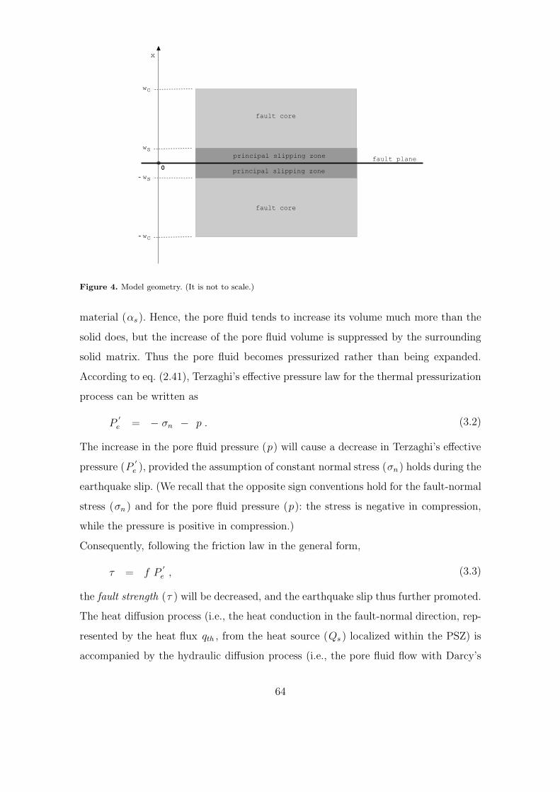
Figure 4. Model geometry. (It is not to scale.)

material (αs ). Hence, the pore fluid tends to increase its volume much more than the

solid does, but the increase of the pore fluid volume is suppressed by the surrounding

solid matrix. Thus the pore fluid becomes pressurized rather than being expanded.

According to eq. (2.41), Terzaghi’s effective pressure law for the thermal pressurization

process can be written as

P′

e = − σn − p . (3.2)

The increase in the pore fluid pressure (p) will cause a decrease in Terzaghi’s effective

pressure (P′

e ), provided the assumption of constant normal stress (σn ) holds during the

earthquake slip. (We recall that the opposite sign conventions hold for the fault-normal

stress (σn ) and for the pore fluid pressure (p): the stress is negative in compression,

while the pressure is positive in compression.)

Consequently, following the friction law in the general form,

τ = f P′

e , (3.3)

the fault strength (τ ) will be decreased, and the earthquake slip thus further promoted.

The heat diffusion process (i.e., the heat conduction in the fault-normal direction, rep-

resented by the heat flux qth , from the heat source (Qs ) localized within the PSZ) is

accompanied by the hydraulic diffusion process (i.e., the pore fluid flow with Darcy’s

64

velocity q in the fault-normal direction). The pore fluid flow is induced by the pore

fluid pressure gradient in the fault-normal direction which arose from the temperature

gradient in the fault-normal direction. For a given time instant, different tempera-

ture changes along the x-coordinate axis induce different pore-fluid pressure changes

along the x-coordinate axis (both due to the thermal expansion phenomenon and the

pore fluid compressibility), thus the pressure gradient is induced in the fault-normal

direction. The situation is illustrated in Fig. 5.

Figure 5. A schematic illustration of the thermal pressurization process mechanism.

Frictional Heating. . The crucial mechanism of the thermal pressurization process

is the frictional heating of the fault. In order to incorporate this mechanism into the

physical model, an appropriate heat source must be chosen. According to the latest

geological findings regarding the extreme thinness of the PSZ, and the theoretical

considerations made by Bizzarri and Cocco (2006a), Rice (2006), Rempel and Rice

(2006), among others, the heat source can be most appropriately represented either

as a finite thickness slipping layer within which the heat is uniformly generated (i.e.,

the PSZ in our model), or as a planar heat source corresponding to the fault plane.

The latter could be a good representation of the heat source for sufficiently long slip

distances, but only if the thickness of the PSZ is small compared to the thickness

65

of hydraulic and thermal boundary layers. This might hold if the PSZ thickness was

about 300 µm or less. Although it is not impossible that the PSZ is so extremely

thin, according to the present knowledge the typical PSZ thickness values are still

higher (≈ 1 mm). Hence, the model of the heat uniformly generated within the finite-

thickness PSZ is adopted here. It corresponds to the situation when the slip rate (∆Vs )

profile across the PSZ is linear, such that the slip rate of the border walls of the PSZ

(i.e., the planes located at x = −ws and x = ws ) equals ∆Vs . The slip rate outside

the PSZ is zero. Then the heat source can be defined as follows (Bizzarri and Cocco,

2006a), (Rempel and Rice, 2006):

Qs ( t ) =τ ( t ) ∆Vs

2 ws; |x| ≤ ws .

Qs = 0 ; |x| > ws ,

(3.4)

Here, the assumption that all the frictional work is converted into the heat was used

(Cardwell et al., 1978), (Scholz, 2002). The above relation can be rewritten according

to the friction law (3.3) as

Qs ( t ) =f P

′

e ∆Vs

2 ws; |x| ≤ ws ,

Qs = 0 ; |x| > ws ,

(3.5)

which can be further rewritten according to Terzaghi’s effective pressure law (3.2) as

follows:

Qs ( t ) = f ( − σn − p ( t ) )∆Vs

2 ws; |x| ≤ ws ,

Qs = 0 ; |x| > ws .

(3.6)

Here, the pore fluid pressure (p) is assumed to be represented by the fault-plane value

at every spatial position within the PSZ, i.e., p (t) = p ( t , x = 0 ). In other words,

p does not vary with the x-coordinate. Such simplification is often used in the physical

models of the thermal pressurization process (Bizzarri and Cocco, 2006a), (Rempel and

Rice, 2006). It should not affect the results considerably, since the typical pore fluid

pressure gradients at the small distances corresponding to the half-width of the PSZ

(≈ 1 mm) are relatively small.

Alternatively to the presented heat source model with a uniform heat generation,

Andrews (2002) has proposed a model with a Gaussian distribution of the heat produc-

tion within the PSZ. However, laboratory experiments performed by Mair and Marone

66

(2000) suggest that the uniform distribution of the heat within the PSZ might be an ap-

propriate heat source representation. Therefore, in agreement with Bizzarri and Cocco

(2006a), Cardwell et al. (1978), and Fialko (2004), we use the uniform heat source in

the model.

3.2.5 Governing Equations

Since the basic assumptions of thermoporoelasticity are adopted in the physical model

(i.e., the solid material is homogeneous and isotropic, and all the pores are intercon-

nected), and we assume that all the processes are reversible, the thermal pressurization

of pore fluid process can be categorized as a thermoporoelastic problem. Therefore, fol-

lowing the discussion on thermoporoelasticity in the previous chapter, the appropriate

set of governing equations should consist of: seven constitutive equations, three force

balance equations, one fluid diffusivity equation, and one thermal diffusivity equation.

The six constitutive equations for the stress variable can be combined with the force bal-

ance equations, thus the number of final governing equations is reduced. According to

the presented geological, laboratory and theoretical assumptions, the equations become

considerably simplified, especially because of the limitation to the one-dimensional

problem and the neglect of body forces.

There are several different ways to formulate the final governing equations for the

thermal pressurization problem, since different dependent and independent variables,

and various material parameters can be used.

Displacement Formulation of Force Balance Equations of Thermal Pres-

surization Process. Similarly as in the isothermal case (2.119), the displacement

formulation of the force balance equations of thermoporoelasticity can be obtained

by combining the six constitutive equations for the stress variable, given by eq. (2.46),

with the force balance equations. Since the body forces are neglected during the thermal

pressurization process, the force balance equations with neglected body forces (2.118)

are used. By combining the constitutive relations with the force balance equations, and

using the total strain definition (2.1), we obtain:

G ∇2ui + ( G + λ )∂ 2uk

∂ xi xk= α

∂ p

∂ xi+

(

λ +2 G

3

)

αb∂ T

∂ xi. (3.7)

In the case of one-dimensional problem (~u = [u; 0; 0 ]), eq. (3.7) reads:

67

( 2 G + λ )∂ 2u

∂ x 2= α

∂ p

∂ x+

(

λ +2 G

3

)

αb∂ T

∂ x. (3.8)

By applying the assumption of incompressible solid material (α = 1), the displace-

ment formulation of the force balance equations of the thermal pressurization process

finally reads:

( 2 G + λ )∂ 2u

∂ x 2=

∂ p

∂ x+

(

λ +2 G

3

)

αb∂ T

∂ x. (3.9)

Alternatively, it can be written in terms of the parameters βb and βvb instead of λ

and G, following the basic relations between poroelastic parameters (see, for example,

Wang, H. (2000)):

∂ 2u

∂ x 2= βv

b

∂ p

∂ x+

βvb

βb

αb∂ T

∂ x. (3.10)

The derived relation (3.10) is in agreement with that proposed by Landau and Lifshitz

(1959).

Fluid Diffusivity Equation of Thermal Pressurization Process. The fluid dif-

fusivity equation of the thermal pressurization process can be derived from the gen-

eral non-linear fluid diffusivity equation of thermoporoelasticity in the one-dimensional

form, given by eq. (2.158).

To obtain it, an expression for the rate of porosity change (∂n/∂t) under conditions

of constant fault-normal stress (σn = 0) in terms of the temperature (T ) and the

pore fluid pressure (p) will be derived in what follows. Subsequently, the obtained

expression will be substituted for the first term in eq. (2.158).

Let us start the derivation with a relation between the Lagrangian porosity (n),

the bulk volumetric strain (εkk ) and the solid volumetric strain (εskk ), which can be

easily derived from the definition of the Lagrangian porostiy (2.8) by using eqs. (2.2)

and (2.5):

n − n0 = εkk − ( 1 − n0 ) εskk . (3.11)

Differentiating the above equation with respect to time leads to the equation:

n = εkk − ( 1 − n0 ) εskk . (3.12)

Then, by performing the time derivatives of the equations defining the bulk volu-

metric strain (2.2) and the solid volumetric (2.5), the following relations are obtained,

68

εkk =Vb

V 0b

, (3.13)

εskk =

Vs

V 0s

, (3.14)

which can be further modified by realizing that under conditions of constant fault-

normal stress (σn = 0), any volume change (i.e., δ Vb , δ Vs or δ Vp ) can be only due

to the change in the pore fluid pressure (p) or in the temperature (T ). Thus we get:

εkk =1

V 0b

(

∂ Vb

∂ p

∂ p

∂ t+

∂ Vb

∂ T

∂ T

∂ t

)

, (3.15)

εskk =

1

V 0s

(

∂ Vs

∂ p

∂ p

∂ t+

∂ Vs

∂ T

∂ T

∂ t

)

. (3.16)

Finally, taking into account eqs. (2.48), (2.54) and (2.69), eq. (3.15) can be rewritten

in terms of the drained bulk compressibility (βb ), the solid bulk compressibility (βs ),

and the solid thermal expansion coefficient (αs ):

εkk = ( βb − βs )∂ p

∂ t+ αs

∂ T

∂ t. (3.17)

Similarly, eq. (3.16) can be rewritten in terms of the Lagrangian porosity in the ini-

tial state (n0 ), the solid bulk compressibility (βs ), and the solid thermal expansion

coefficient (αs ):

εskk =

n0

( 1 − n0 )βs

∂ p

∂ t+ αs

∂ T

∂ t. (3.18)

Here, we have used Betti-Maxwell reciprocal theorem, i.e., the equality

∂ Vb

∂ p| σ = 0 =

∂ Vp

∂ σ| p = 0 , (3.19)

which postulates that the change in the bulk volume (Vb ) due to the change in the pore

fluid pressure (p) is equal to the change in the pore volume (Vp ) due to the change

in the mean total stress (σ ) which is of equal value as the pore fluid pressure (p)

(Detournay and Cheng, 1993).

After substituting eqs. (3.17) and (3.18) into eq. (3.12), and performing some al-

gebraic manipulations, we obtain the desired relation for the rate of porosity change

under conditions of constant fault-normal stress (σn = 0):

n = ( βb − ( 1 + n0 ) βs )∂ p

∂ t+ n0 αs

∂ T

∂ t. (3.20)

We note that the obtained relation (3.20) is in agreement with that proposed by Ghabe-

zloo and Sulem (2008a).

69

Finally, after the substitution of eq. (3.20) into eq. (2.158), and performing some

mathematical manipulations, the desired fluid diffusivity equation of the thermal pres-

surization process is obtained in the form:

∂ p

∂ t( βb + n0 βf − ( 1 + n0 ) βs ) +

∂ T

∂ tn0 ( αs − αf ) −

−∂

∂ x

[

k

µ

∂ p

∂ x

]

−k

µβf

(

∂ p

∂ x

)2

+k

µαf

(

∂ p

∂ x

)(

∂ T

∂ x

)

= 0 .

(3.21)

An important comment should be made here. The same relation for the rate of

porosity change as (3.20) would be obtained by using the force balance equation of

the thermal pressurization process (3.10) together with eqs. (3.11) and (3.18) and

some relevant relations between poroelastic parameters. We have used another way of

derivation because it seemed more straightforward to us.

Thermal Diffusivity Equation of Thermal Pressurization Process. The one-

dimensional thermal diffusivity equation of thermoporoelasticity in the general non-

linear form (2.177) is directly applicable as the thermal diffusivity equation of the

thermal pressurization process:

∂

∂ x

(

kth∂ T

∂ x

)

+ ρf cfk

µ

(

∂ p

∂ x

) (

∂ T

∂ x

)

+ n αf T∂ p

∂ t−

− αfk

µT

(

∂ p

∂ x

)2

+ Qs = ce∂ T

∂ t.

(3.22)

After the substitution for the heat source (Qs ) in the above equation according to eq.

(3.6), the thermal diffusivity equation (3.22) can be rewritten in the form:

∂

∂ x

(

kth∂ T

∂ x

)

+ ρf cfk

µ

(

∂ p

∂ x

) (

∂ T

∂ x

)

+ n αf T∂ p

∂ t−

− αfk

µT

(

∂ p

∂ x

)2

+ f ( − σn − p )∆Vs

2 ws

= ce∂ T

∂ t; |x| ≤ ws ,

∂

∂ x

(

kth∂ T

∂ x

)

+ ρf cfk

µ

(

∂ p

∂ x

) (

∂ T

∂ x

)

+ n αf T∂ p

∂ t−

− αfk

µT

(

∂ p

∂ x

)2

= ce∂ T

∂ t; |x| > ws .

(3.23)

Simplified Governing Equations for Thermal Pressurization Process. The

governing equations derived so far, given by (3.21) and (3.22), can be further simplified.

First, applying the assumption of spatially constant permeability (k ) and dynamic

70

fluid viscosity (µ), and the assumption of time constant porosity (n), the governing

equations for the pore fluid pressure and temperature variations respectively read:

∂ p

∂ t( βb + n0 βf − ( 1 + n0 ) βs ) +

∂ T

∂ tn0 ( αs − αf ) −

−k

µ

∂ 2p

∂ x2−

k

µβf

(

∂ p

∂ x

)2

+k

µαf

(

∂ p

∂ x

)(

∂ T

∂ x

)

= 0 ,(3.24)

kth∂2 T

∂ x2+ ρf cf

k

µ

(

∂ p

∂ x

) (

∂ T

∂ x

)

+ n0 αf T∂ p

∂ t−

− αfk

µT

(

∂ p

∂ x

)2

+ Qs = ce∂ T

∂ t.

(3.25)

Now, using the assumption of incompressible solid material, i.e., βs = 0, and the fact

that the pore fluid thermal expansivity (αf ) is about two orders of magnitude greater

than the solid thermal expansivity (αS ) (see Tab. 2), the first governing equation (3.24)

can be simplified. A further simplification consists in realizing that the value of n0 βf

is slightly larger than the value of βb , hence the first term in eq. (3.24) can be further

simplified (see Tabs. 2 and 3). The governing equations then read:

∂ p

∂ tn0 βf −

∂ T

∂ tn0 αf −

k

µ

∂ 2p

∂ x2−

k

µβf

(

∂ p

∂ x

)2

+

+k

µαf

(

∂ p

∂ x

)(

∂ T

∂ x

)

= 0 ,

(3.26)

kth∂2 T

∂ x2+ ρf cf

k

µ

(

∂ p

∂ x

) (

∂ T

∂ x

)

+ n0 αf T∂ p

∂ t−

− αfk

µT

(

∂ p

∂ x

)2

+ Qs = ce∂ T

∂ t.

(3.27)

Non-dimensionalisation of Governing Equations and Quantification of Indi-

vidual Terms. The governing equations for the thermal pressurization process (3.26),

(3.27) are non-linear equations. They are difficult to solve even numerically. Therefore,

we transform them into a non-dimensional form and quantify the individual terms, in

order to investigate whether a further simplification of them by omitting small terms

can be made.

In order to transform the governing equations into a non-dimensional form, non-

dimensional variables must be introduced. There are four variables appearing in the

governing equations (3.26) and (3.27). Two of them are independent variables (the

71

time t and the position x), and two are dependent variables (the pore fluid pressure

p = p (x, t) and the temperature T = T (x, t)). The four non-dimensional variables

are thus defined - the non-dimensional pressure (Π ), the non-dimensional temperature

(Θ ), the non-dimensional time (τ ), and the non-dimensional position (ξ ),

Π =p

pch

,

Θ =T

Tch,

τ =t

tch,

ξ =x

xch,

(3.28)

where pch , Tch , tch , and xch denote, respectively, the characteristic pore fluid pres-

sure, the characteristic temperature, the characteristic time, and the characteristic

length scale of the thermal pressurization of pore fluid process. In addition, the non-

dimensional Terzaghi’s effective pressure (Π′

) is introduced, in order to put the heat

source term (Qs ) into a dimensionless form,

Π′

=P′

e

P ′

ech

, (3.29)

where P′

echis the characteristic Terzaghi’s effective pressure.

Values of the characteristic quantities are chosen as follows. The total slip duration

at a point (ttot ) is taken as the characteristic time (tch ) value. The characteristic

pore fluid pressure (pch ), the characteristic temperature (Tch ), and the characteristic

Terzaghi’s effective pressure (P′

ech) values are chosen as the time-averaged values of

the pore fluid pressure (p), temperature (T ), and Terzaghi’s effective pressure (P′

e ),

respectively, during the total slip duration at a fault point (ttot ) (see Tabs. 3 and 1).

The characteristic length scale (xch ) value is assumed to be represented by the typical

distance from the fault plane that is reached by the pore fluid pressure front during

the total slip duration at a point, i.e., by the characteristic thickness of the hydraulic

boundary layer (Lachenbruch, 1980). According to Tabs. 1 and 3, the characteristic

values are

72

pch = 1.3 × 108 Pa ,

Tch = 103 K ,

xch = 10−2 m ,

tch = 10 s ,

P′

ech= 63 × 106 Pa .

(3.30)

After the substitution for p, T , t, x, and Qs in the governing equations (3.26) and

(3.27) according to (3.28) we obtain:

n0 βf∂ ( pch Π )

∂ ( tch τ )− n0 αf

∂ ( Tch Θ )

∂ ( tch τ )−

k

µ

∂ 2( pch Π )

∂ ( xch ξ )2 −

−k

µβf

{

∂ ( pch Π )

∂ ( xch ξ )

}2

+k

µαf

∂ ( pch Π )

∂ ( xch ξ )

∂ ( Tch Θ )

∂ ( xch ξ )= 0 ,

(3.31)

kth∂2 ( Tch Θ )

∂ ( xch ξ )2 + ρf cfk

µ

∂ ( pch Π )

∂ ( xch ξ )

∂ ( Tch Θ )

∂ ( xch ξ )− ce

∂ ( Tch Θ )

∂ ( tch τ )+

+ n0 αf ( Tch Θ )∂ ( pch Π )

∂ ( tch τ )− αf

k

µ( Tch Θ )

{

∂ ( pch Π )

∂ ( xch ξ )

}2

+

+f ∆Vs

2 ws

P′

echΠ′

= 0 .

(3.32)

Here, the heat source definition (3.5) was used to make the substitution for Qs possible.

Now, we will introduce an expression for the characteristic time (tch ) in terms of

another parameters or characteristic quantities. In order to derive such expression,

every two linear terms in the governing equations which contain the characteristic time

are put into equality, from which the relation for tch is thus found (for each couple of

terms). Finally, the relevant values from Tabs. 2 and 3 are substituted into the obtained

expressions. The expression for which the calculated characteristic time value is about

10 s (which is the value corresponding to the anticipation, see (3.30)), is chosen as the

proper expression for the characteristic time (tch ). Thereby the expression is obtained

by putting the first and the third term on the l.h.s. of eq. (3.31) into equality. It reads:

tch = n0 βfµ

kx2

ch . (3.33)

Taking into account eq. (2.101), the above relation can be rewritten in terms of the

hydraulic diffusivity (αhy ). Under conditions of time constant porosity (n), eq. (3.33)

in terms of αhy reads:

73

tch =x2

ch

αhy. (3.34)

Now, the obtained relation (3.33) is substituted for the characteristic time (tch ) in

the governing equations (3.31), (3.32). By multiplying eq. (3.31) with (µ x2ch) / (k pch)

and eq. (3.32) with x2ch/ (kth Tch), using the thermal diffusivity (αth ) definition (2.114),

and eq. (2.101) for the hydraulic diffusivity (αhy ), the dimensionless governing equa-

tions are obtained in the form:

∂ Π

∂ τ−

αf Tch

βf pch

∂ Θ

∂ τ−

∂ 2Π

∂ ξ2− βf pch

(

∂ Π

∂ ξ

)2

+

+ αf Tch

(

∂ Π

∂ ξ

) (

∂ Θ

∂ ξ

)

= 0 ,

(3.35)

∂2Θ

∂ ξ 2+ Pe

(

∂ Π

∂ ξ

) (

∂ Θ

∂ ξ

)

−αhy

αth

∂ Θ

∂ τ+

n0 αf pch αhy

kth

Θ∂ Π

∂ τ−

−αf k p

2ch

µ kthΘ

(

∂ Π

∂ ξ

)2

+f ∆Vs P

′

echx2

ch

2 ws kth TchΠ′

= 0 .

(3.36)

Here, Pe denotes the so-called Peclet number (Lee and Delaney, 1987), defined as

Pe =ρf cf k pch

µ kth

. (3.37)

Let us make the following denotations of the dimensionless groups of quantities in eqs.

(3.35) and (3.36):

A =αf Tch

βf pch

,

B = βf pch ,

C = αf Tch ,

D =αhy

αth

,

E =n0 αf pch αhy

kth,

F =αf k pch

µ kth,

G =f ∆Vs P

′

echx2

ch

2 ws kth Tch

.

(3.38)

According to (3.38), the governing equations (3.35) and (3.36) can be rewritten as

74

∂ Π

∂ τ− A

∂ Θ

∂ τ−

∂ 2Π

∂ ξ2− B

(

∂ Π

∂ ξ

)2

+

+ C

(

∂ Π

∂ ξ

) (

∂ Θ

∂ ξ

)

= 0 ,

(3.39)

∂2Θ

∂ ξ 2+ Pe

(

∂ Π

∂ ξ

) (

∂ Θ

∂ ξ

)

− D∂ Θ

∂ τ+ E Θ

∂ Π

∂ τ−

− F Θ

(

∂ Π

∂ ξ

)2

+ G Π′

= 0 .

(3.40)

The individual terms in eq. (3.39) are respectively from left to right of order 1, A, 1,

B , and C . Similarly, the terms in eq. (3.40) are of order 1, Pe, D , E , F , and G. To

quantify the order of the individual terms in the governing equations, a substitution of

the relevant values into (3.38) according to Tabs. 1, 2, and 3 is made,

A =(2.5 × 10−3 K−1) (103 K)

(4.5 × 10−9 Pa−1) (1.3 × 108 Pa)≈ 4.2

B = (4.5 × 10−9 Pa−1) (1.3 × 108 Pa) ≈ 0.6

C = (2.5 × 10−3 K−1) (103 K) ≈ 2.5

Pe =(340 kg m−3) (2.3 × 103 J kg−1 K−1) (10−19 m2) (1.3 × 108 Pa)

(5.7 × 10−5 Pa s) (1.35 J s−1 m−1 K−1)

≈ 0.13

D =10−5 m2 s−1

0.5 × 10−6 m2 s−1≈ 20

E =0.04 (2.5 × 10−3 K−1) (1.3 × 108 Pa) (10−5 m2 s−1)

1.35 J s−1 m−1 K−1≈ 0.1

F =(2.5 × 10−3 K−1) (10−19 m2) (1.69 × 1016 Pa2)

(5.7 × 10−5 Pa s) (1.35 J s−1 m−1 K−1)≈ 5.46 × 10−2

G =0.45 (1 m s−1) (63 × 106 Pa) (10−4 m2)

2 (1 × 10−3 m) (1.35 J s−1 m−1 K−1) (103 K)≈ 103 .

(3.41)

The corresponding terms in the governing equations (3.39), (3.40) are thus of the

following orders:

A ∝ 1 , B ∝ (0.1 ; 1) , C ∝ 1 , P e ∝ 0.1

D ∝ 10 , E ∝ 0.1 , F ∝ 0.1 , G ∝ 103 .

(3.42)

75

The first and the most unexpected result of the analysis regarding the governing

equation for the pore fluid pressure variation (3.39) is that at least one non-linear term

cannot be omitted in the equation. Commonly, all the non-linear terms are omitted

and the linearized form of (3.39) is used as the governing equation for the thermal

pressurization process. However, our analysis shows that the non-linear term containing

the coefficient C is of the same order as the linear terms in the equation. Furthermore,

the non-linear term containing the coefficient B is either of the same order or by one

order smaller than the linear terms. Because of the uncertainty in values of various

parameters used to determine the order of the terms, we do not neglect either of

the non-linear terms. Hence, the dimensionless governing equation for the pore fluid

pressure variation is the original non-linear eq. (3.39), now rewritten with the terms

arranged according to their order:

∂ Π

∂ τ− A

∂ Θ

∂ τ−

∂ 2Π

∂ ξ2+ C

(

∂ Π

∂ ξ

)(

∂ Θ

∂ ξ

)

− B

(

∂ Π

∂ ξ

)2

= 0 . (3.43)

Here, the first four terms are of the same order. The second and third linear terms are

the source and the transport terms, respectively. The terms containing the coefficient

C and B represent the change in pore fluid mass respectively due to the the thermal

expansion and due to the compression of the pore fluid along the flow path (Mase and

Smith, 1985).

The second result of the performed dimensional analysis is that the nonlinear term

containing Peclet number (Pe), and the coupling terms containing the coefficients

E and F can be neglected in the governing equation for the temperature variation

(3.40), since they are of relatively small orders. Consequently, the non-linear governing

equation (3.40) becomes linear. Physically, the omission of the term containing Peclet

number means that the convective heat transport is neglected. The omission of the

terms containing coefficients E and F means that the heating due to the reversible

work done on the fluid (Mase and Smith, 1985) is not taken into account. The resultant

dimensionless governing equation for the temperature variation hence reads:

G Π′

− D∂ Θ

∂ τ+

∂2Θ

∂ ξ 2= 0 . (3.44)

Here, the terms are arranged according to their order. The first term, which represents

the heat source, is the highest order term. The second term represents the heat storage.

76

The last term is the smallest order term in the equation and is often referred to as the

transport term (Lachenbruch, 1980). It represents the conductive transport of heat.

The obtained linearized equation (3.44) has a very advantageous form. If a planar

heat source confined to the fault plane was used in the model (instead of the proposed

more realistic one that is confined to the finite-thickness PSZ), the heat source can be

introduced through a boundary condition. Hence, the heat source term (G Π′

) vanishes

in the equation, hence the equation becomes uncoupled from the second governing

equation for the pore fluid pressure variation (3.43). Consequently, the equation for

the temperature variation can be solved independently from the pressure diffusion

equation. Its solution is then used to solve the governing equation for the pore fluid

pressure variation.

Final Governing Equations of Thermal Pressurization of Pore Fluid Process.

Following the preceding dimensional analysis and the derived governing equations given

by (3.26) and (3.27), we propose the following final governing equations for the thermal

pressurization of pore fluid process,

∂ p

∂ tn0 βf −

∂ T

∂ tn0 αf −

k

µ

∂ 2p

∂ x2−

k

µβf

(

∂ p

∂ x

)2

+

+k

µαf

(

∂ p

∂ x

)(

∂ T

∂ x

)

= 0 ,

(3.45)

kth∂2 T

∂ x2+ Qs = ce

∂ T

∂ t, (3.46)

where the heat source is non-zero (Qs 6= 0) only within the PSZ ( |x| ≤ ws ).

The second governing equation (3.46), which is the equation for the temperature

variation, is identical to the commonly used equation in the models of the thermal

pressurization of pore fluid process during earthquake slip (Andrews, 2002), (Bizzarri

and Cocco, 2006a), (Rempel and Rice, 2006), (Rice, 2006), (Segall and Rice, 2006).

However, the first governing equation (3.45), which is the equation for the pore fluid

pressure variation, differs from the commonly used equation - it contains additionally

two non-linear terms, which cannot be generally neglected according to the presented

dimensional analysis.

77

3.2.6 Primary Shortcomings of the Presented Model

1. Plasticity is not taken into account (only the elasticity is considered).

Especially the local stresses at the propagating rupture front may be sufficiently

high to cause irreversible changes in material properties and inelastic deformations

which are detected in the fault gouge materials (Poliakov et al., 2002), (Andrews,

2005), (Rice and Cocco, 2006). The effect becomes considerable especially as the

rupture propagation velocity approaches the Rayleigh velocity (Rice and Cocco,

2006). The high rupture front stresses may cause the dilatancy of the material

(inelastic pore volume increase) leading to the significant increase in permeability

(due to its strong dependence on porosity), thus reducing the pore fluid pressure

and increasing the material strength (Viesca et al., 2008). The studies, however,

suggest that dilatancy is important during a nucleation phase of the rupture (when

the highest stress concentrations exist at the rupture front), but it has a negligible

effect after a steady slipping is developed (Segall and Rice, 1995). Then, the fric-

tional heating, possibly accompanied by the thermal pressurization of pore fluid,

is the primary mechanism acting on the fault. Since the dilatancy seems to have a

negligible effect during the thermal pressurization process, omitting the dilatancy

in the physical model should not distort the results significantly.

2. The material is assumed to be macroscopically homogeneous, i.e., the values of

material parameters are spatial constants.

The validity of this assumption is questionable particularly due to the large spatial

variations in the permeability value in the fault-normal direction. However, since

the thermal pressurization process effectively occurs only at relatively small fault-

normal length scales, such assumption might be admissible.

3. Values of material parameters are assumed to be constant during the earthquake

slip.

This is surely not true especially for the porosity (n), permeability (k ), pore fluid

density (ρf ), pore fluid viscosity (µ), pore fluid compressibility (βf ), pore fluid ther-

mal expansivity (αf ), drained bulk compressibility (βb ), and hydraulic diffusivity

(αhy ), which are the most sensitive parameters to changes in the pore fluid pres-

sure and temperature. The assumption might hold and the usage of time-averaged

78

values might be admissible under conditions that the variations in parameters are

relatively small and linear. However, there is some evidence that the variations

becomes non-linear at high pressures and temperatures of interest (e.g., the pore

fluid compressibility (βf ) variation with pressure becomes considerably non-linear

at the temperatures higher than about 500 K (Marshall, 2008)). Nevertheless, fur-

ther experiments are needed in order to incorporate the variations properly into the

physical model.

4. Anisotropy is not taken into account.

The presented analysis is based both on the assumption that the bulk material

is isotropic, and that the poroelastic response of the material is purely isotropic.

The latter assumption means that the poroelastic response of the material follows

the theory of poroelasticity introduced by Biot (1941), which predicts that for

an isotropic material, only the changes in the normal stress components (and not

those in the shear stress components) can induce a pore fluid pressure change or

cause a volumetric deformation of the rock. However, there are some theoretical

investigations and laboratory experiments suggesting that a pore fluid pressure

response to the applied shear stress is possible, with a dominant elastic response,

and increasing with the increasing applied shear stress (Skempton, 1954), (Wang,

1997), (Lockner and Stanchits, 2002). It appears to be the result of a stress-induced

anisotropy of the material. The first assumption of the bulk material isotropy is

the more inaccurate one, since several geologic observations imply that fault zone

rocks have typically anisotropic material properties. Especially the anisotropy in the

permeability is significant - the permeability in the fault-parallel direction can be

even 3 orders of magnitude higher than that in the fault normal direction (Faulkner

and Rutter, 2005).

5. The model is kinematic.

We do not consider the dynamic effects, e.g., the effect of the fault strength (τ )

variations on the slip rate (∆Vs ), and thus on the heat source (Qs ), is not taken

into account.

6. Chemical effects are not considered.

79

Various studies suggest that the effect of coseismic chemical interactions between

the pore fluid and the solid material of the rock is non-negligible, thus should be

incorporated into the physical model of the thermal pressurization process. Particu-

larly the thermally induced dehydration of the rock hydrous minerals (e.g., clay-rich

minerals) possibly acts as an additional source term in the governing equation for

the pore fluid pressure variation of the thermal pressurization process (Hirose and

Bystricky, 2007), (Brantut et al., 2008). Furthermore, the chemical reactions may

consume a significant amount of the frictional heat generated during earthquake

slip, and thereby suppress the temperature rise (and hence suppress melting). Un-

der sufficiently high concentrations of reactive materials, the frictional heat con-

sumption could possibly reach 50 % of the frictional heat generated during slip

(Hamada et al., 2009). The chemical effects can also contribute to the explanation

of the heat flow paradox (Jacobs et al., 2006). Thus the chemical effects might be

taken into account in the future thermal pressurization models.

7. Pure water is assumed to be the pore fluid. Moreover, we assume that the water

exists in a single phase.

The first assumption is surely not satisfied under real fault conditions. The pore

fluid typically consists of a water solution containing Na, Cl−1 , Sr , SO2−4 , among

others, which could possibly change the pore fluid behavior and its chemical in-

teractions with the rock during the thermal pressurization process. The second

assumption on the water phase is also a matter of debate. For example, under hy-

drostatic conditions, assuming the normal geothermal gradient (30 K per kilometer

of depth) and the typical seismogenic depth (7 km), the liquid water should un-

dergo a phase change into a supercritical state during the thermal pressurization

of pore fluid process. The critical point of water (647 K , 22 MPa) is exceeded

during the large temperature and pore fluid pressure changes (Chaplin, 2009). The

phase change into the supercritical state could significantly affect some of the wa-

ter properties. For example, the supercritical water is highly compressible, implying

that even small changes in pressure can induce large changes in the water density

(ρf ), thus affecting its viscosity (µ) and solvation properties in chemical reactions

with the rock. Moreover, experiments performed with granite show a rapid increase

80

in permeability (k ) when the critical temperature of water is reached (647 K ),

which may be due to a micro-fracture network generation under supercritical water

conditions (Takahashi et al., 2003).

3.3 Main Points of Controversy and Open Questions

Although the thermal pressurization of pore fluid process during earthquake slip has

been known and studied for more than a quarter-century, there are still some contro-

versial issues on it. Particularly the following two points are still a matter of debate:

1. The effective stress principle lacks a laboratory verification at coseismic slip rates.

2. The connectivity of the porous rock space can be lost during the interseismic period,

for example due to the mineralization of the rock (Rice, 2006). However, although

in the case that the hypothesis holds, there are some studies suggesting that co-

seismic stress concentrations at the rupture tip are possibly high enough to induce

a reconnection of the pores (Poliakov et al., 2002). If the rock connectivity was

corrupted, the classical theory of poroelasticity would not be applicable since it is

built on the assumption of the porous space interconnection.

81

4 Conclusions

In this thesis, we summarized the most important dynamic fault weakening mechanisms, briefly cha-

racterized them, and assessed their possible contributions to the dynamic fault

weakening during tectonic earthquakes, presented an introductory text on the theory of thermoporoelasticity, starting with

a detailed development of the theory of linear poroelasticity, following with its

extension to a thermoporoelastic case, and including a detailed derivation of the

general non-linear governing equations of thermoporoelasticity, summarized the latest geological, laboratory, and theoretical results regarding the

thermal pressurization of pore fluid process, proposed a set of appropriate values of the parameters relevant for the thermal

pressurization of pore fluid process, proposed a modified physical model of the thermal pressurization of pore fluid

process, following the recent field results and the theory of thermoporoelasticity.

By modifying the general non-linear governing equations of thermoporoelasticity

according to the properties of the physical model of the thermal pressurization of pore

fluid process, we obtained the governing equations adequate for the process. Then, we

transformed them into a non-dimensional form, and quantified the individual terms.

The non-dimensionalisation shows that the governing equation for the temperature variations can be used in its linearized

form, the governing equation for the pore fluid pressure variations, however, cannot be

used in its linearized form, since at least one non-linear term cannot be neglected

in the equation, as being of the same order of magnitude as the linear terms in the

equation.

Commonly, both governing equations are applied in their linear form. Our analysis,

however, implies that one of the equations should be used in its original non-linear

form. We admit that our results may be slightly inaccurate, as a consequence of the

82

considerable uncertainty in values of various model parameters. Nevertheless, just due

to the latter fact, we guess that the non-linear form of the governing equation for the

pore fluid pressure variations should be used as the proper governing equation for the

thermal pressurization process.

83

References

Archard, J. F., 1958-1959. The temperature of rubbing surfaces. Wear 2, 438–455.

Andrews, D. J., 2002. A fault constitutive relation accounting for thermal pressur-

ization of pore fluid. J. Geophys. Res. 107B12, 2363, doi:10.1029/2002JB001942.

Andrews, D. J., 2005. Rupture dynamics with energy loss outside the slip zone. J.

Geophys. Res. 110(B1), 1307.

Arsenin, V. J., 1977. Matematicka fyzika. Alfa.

Batchelor, G. H., 1967. An Introduction to Fluid Dynamics. Cambridge University

Press.

Bear, J., 1988. Dynamics of Fluids in Porous Media. Courier Dover Publications.

Beeler, N. M., and T. E. Tullis, 2003. Constitutive relationships for fault strength

due to flash-heating. SCEC Annual Meeting Proceedings and Abstracts XIII, p.66.

Bejan, A., I. Dincer, S. Lorente, A. F. Miguel, and A. H. Reis, 2004. Porous

and complex flow structures in modern technologies. Springer, ISBN 0387202250.

Berryman, J. G., 1992. Effective stress for transport properties of inhomogeneous

porous rock. Journal of Geophysical Research 97, 17409-17424.

Biot, M. A., 1941. General theory of three-dimensional consolidation. Journal of

Applied Physics 12, 155-164.

Biot, M. A., 1955. Theory of elasticity and consolidation for a porous anisotropic

solid. Journal of Applied Physics 26, 182-185.

Biot, M. A., 1956. General solutions of the equations of elasticity and consolidation

for a porous material. J. Appl. Mech., Trans. ASME 78, 91-96.

Biot, M. A., 1956. Thermoelasticity and irreversible thermodynamics. Journal of

Applied Physics 27, 240-253.

Biot, M. A., 1962. Theory of propagation of elastic waves in a fluid-saturated porous

solid; part I: low frequency range and part II: higher frequency range. Journal of the

Acoustical Society of America 28, 168-178 and 179-191.

Biot, M. A., 1962. Mechanics of deformation and acoustic propagation in porous

media. Journal of Applied Physics 33, 1482—1498.

84

Biot, M. A., 1973. Nonlinear and semilinear rheology of porous solids. J. Geophys.

Res. vol.78, no.23, 4924-4937.

Biot, M. A. and D. G. Willis, 1957. The elastic coefficients of the theory of

consolidation. J. Appl. Mech. 24, 594-601.

Bizzarri, A. and M. Cocco, 2003. Slip-weakening behavior during the propagation

of dynamic ruptures obeying to rate- and state-dependent friction laws. J. Geophys.

Res. 108, 2373.

Bizzarri, A. and M. Cocco, 2006. A thermal pressurization model for the sponta-

neous dynamic rupture propagation on a three-dimensional fault: 1. Methodological

approach. J. Geophys. Res. 111, B05303, doi:10.1029/2005JB003862.

Bizzarri, A. and M. Cocco, 2006. A thermal pressurization model for

the spontaneous dynamic rupture propagation on a three-dimensional fault:

2. Traction evolution and dynamic parameters. J. Geophys. Res.111, B05304,

doi:10.1029/2005JB003864.

Bowden, F. P. and D. Tabor, 1950. The Friction and Lubrication of Solids. Claren-

don Press, Oxford, Part I, 52-57.

Brantut, N., A. Schubnel, and J. Corvisier, 2008. Thermo-Chemical Pressuriza-

tion of Fault Gouges During Coseismic Slip. AGU, Fall Meeting 2008, abstract.

Brodsky, E. E. and H. Kanamori, 2001. Elastohydrodynamic lubrication of faults.

J. Geophys. Res. 106, 16357–16374.

Brune, J. N., S. Brown, and P. A. Johnson, 1993. Rupture mechanism and

interface separation in foam rubber models of earthquakes: A possible solution to

the heat flow paradox and the paradox of large overthrusts. Tectonophysics 218,

59-67.

Burridge, R. and L. Knopoff, 1967. Model and theoretical seismicity. Bull. Seismol.

Soc. Am. 57, 341-371.

Cardwell, R. K., D. S. Chinn, G. F. Moore, and D. L. Turcotte, 1978.

Frictional heating on a fault zone with finite thickness. Geophys J. R. Astron. Soc.

52, 525–530.

Chaplin, M., 2009. Available at http://www.lsbu.ac.uk/water/phase.html.

85

Charlez, P. A., 1991. Rock Mechanics, vol. 1, Theoretical Fundamentals. Editions

Technip, Paris.

Chester, J. S., F. M. Chester, and A. K. Kronenberg, 2005. Fracture surface

energy of the Punchbowl Fault, San Andreas System. Nature 437, 133–136.

Cocco, M. and A. Bizzarri, 2004. Dynamic fault weakening caused by thermal pres-

surization in an earthquake model governed by rate- and state-dependent friction.

EOS, Trans. AGU 85, Fall Meeting Suppl., Abstract T22A-06.

Cocco, M., P. Spudich, and E. Tinti, 2006. On the mechanical work absorbed on

faults during earthquake ruptures. Revised Version for the AGU Monograph on Ra-

diated Energy and the Physics of Earthquakes Faulting, A. McGarr, R. Abercrombie,

H. Kanamori and G. di Toro, Eds.

Coussy, O., 2004. Poromechanics John Wiley and Sons

Delaney, P. T., 1982. Rapid intrusion of magma into wet rocks: Groundwater flow

due to pore pressure increases. J. Geophys. Res. 87, 7739–7756.

Detournay, E. and A. H.-D. Cheng, 1993. Fundamentals of poroelasticity, Chapter

5 in Comprehensive Rock Engrg., vol. II., Pergamon Press, J. Hudson, ed., 113-169.

Di Toro, G., D. L. Goldsby, and T. E. Tullis, 2004. Friction falls toward zero in

quartz rock as slip velocity approaches seismic rates. Nature 427, 436–439.

Di Toro, G., T. Hirose, S. Nielsen, G. Pennacchioni, and T. Shimamoto,

2006. Natural and experimental evidence of melt lubrication of faults during earth-

quakes. Science 311, 647-649.

Engineeringtoolbox, 2009. Available at

http://www.engineeringtoolbox.com/water-thermal-properties-d 162.html.

Faulkner, D. and E. Rutter, 2005. On the maintenance of high fluid pressures in

large fault zones. Geophysical Research Abstracts, vol. 7.

Fauvel, E., Ch. Joussot-Dubien, P. Guichardon, G. Charbit, F. Charbit,

and S. Sarrade, 2004. A double-wall reactor for hydrothermal oxidation with

supercritical water flow across the inner porous tube. The Journal of supercritical

fluids 28, 47-56.

Fialko, Y., 2004. Temperature fields generated by the elastodynamic propagation of

shear cracks in the Earth. J. Geophys. Res. 109, B01303, doi: 10.1029/2003JB002497.

86

Foster, R. J., 1985. Geology (Fifth Edition). Charles E. Merrill Publishing Company.

Ghabezloo, S. and J. Sulem, 2008. Stress dependent thermal pressurization of a

fluid-saturated rock. Rock Mechanics and Rock Engineering 42 (1), 1-24.

Ghabezloo, S. and J. Sulem, 2008. Experimental study of thermal pressurization

phenomenon in geomaterials. Alert Workshop 2008, Abstract.

Goldsby, D. L., and T.E. Tullis, 2002. Low frictional strength of quartz rocks at

subseismic slip rates. Geophys. Res. Lett..

Gueguen, Y. and M. Bouteca, 2004. Mechanics of fluid saturated rocks. Interna-

tional Geophysics Series, vol. 89. Elsevier Academic Press.

Hamada, Y., T. Hirono, W. Tanikawa, W. Soh, and S.-R. Song, 2009. Energy

taken up by co-seismic chemical reactions during a large earthquake: An example

from the 1999 Taiwan Chi-Chi earthquake. Geophys. Res. Lett. 36.

Harris, R. A. and S. M. Day, 1997. Effects of a low - velocity zone on a dynamic

rupture. Bull. Seism. Soc. Am. 87, 1267-1280.

Heaton, T. H., 1990. Evidence for and implications of self-healing pulses of slip in

earthquake rupture. Phys. Earth. Planet. Inter. 64, 1–20.

Hirose, T. and M. Bystricky, 2007. Extreme dynamic weakening of faults during

dehydration by coseismic shear heating. Geophys. Res. Lett. 34, L14311.

Jacobs, J. R., J. P. Evans, and P. T. Kolesar, 2006. Energentics of chemical alter-

ation in fault zones and its relationship to the seismic cycle. Geophysical monograph

- AGU, Vol. 170, 181-191.

Jeffreys, H., 1942. On the mechanics of faulting. Geol. Mag. 79, 291–295.

Kanamori, H. and E. E. Brodsky, 2001. The physics of earthquakes. Phys. Today

54, 34-39.

Kanamori, H. and T. H. Heaton, 2000. Microscopic and macroscopic physics of

earthquakes. Geophys. Monogr. Ser., AGU 120, 147–163.

Kirkpatrick, J. D., Z. K. Shipton, and C. Persano, 2009. Pseudotachylytes;

rarely generated, rarely preserved, or rarely reported? Bull. Seism. Soc. Am. 99, no.

1, 382-388.

Lachenbruch, A. H., 1980. Frictional heating, fluid pressure, and the resistance to

fault motion. J. Geophys. Res. 85, 6097–6122.

87

Landau, I. and E. Lifshitz, 1959. Theory of Elasticity. Translated from Russian by

J. Sykes and W. Reid. Addison-Wesley, Reading, Mass..

Lapusta, N. and J. R. Rice, 2003. Low-Heat and Low-Stress Fault Operation in

Earthquake Models of Statically Strong but Dynamically Weak Faults. AGU, Fall

Meeting 2003 abstract.

Lee, Tien-Chang, P. T. Delaney, 1987. Frictional heating and pore pressure rise

due to a fault slip. Geophysical Journal International 88, 569-591.

Lockner, D., R. Summers, and J. Byerlee, 1986 Effects of temperature and

sliding rate of frictional strength of granite. Pure Appl. Geophys. 124, 445–469.

Lockner, D., H. Naka, H. Tanaka, H. Ito, and R. Ikeda, 2000 Permeability

and strength of core samples from the Nojima fault of the 1995 Kobe earthquake. In

Proceedings of the International Workshop on the Nojima Fault Core and Borehole

Data Analysis, ed. H. Ito et al., U.S. Geol. Surv. Open File Rep. 00-129, 147–152.

Lockner, D. A., and S. A. Stanchits, 2002 Undrained poroelastic response of

sandstones to deviatoric stress change. J. Geophys. Res. 107(B12), 2353.

Mair, K. and C. J. Marone, 1999. Friction of simulated fault gouge for a wide

range of slip velocities and normal stresses. J. Geophys. Res. 104, 28899-28914.

Mair, K. and C. J. Marone, 2000. Shear heating in granular layers. Pure Appl.

Geophys. 157, 1847–1866.

Marone, C. J., 1998. Laboratory-derived friction laws and their application to seis-

mic faulting. Ann. Revs. Earth and Plan. Sci. 26, 643-696.

Marshall, S. L., 2008. Nonlinear Pressure Diffusion in Flow of Compressible Liquids

Through Porous Media. Transport in Porous Media 77, 431-446.

Mase, C. W. and L. Smith, 1985. Pore-fluid pressures and frictional heating on a

fault surface. Pure Appl. Geophys. 122, 583–607.

Mase, C. W. and L. Smith, 1987. Effects of frictional heating on the thermal,

hydrologic, and mechanical response of a fault. J. Geophys. Res. 92, 6249–6272.

McKenzie, D. P., and J. N. Brune, 1972. Melting on fault planes during large

earthquakes. Geophys. J. R. Astron. Soc. 29, 65–78.

McTigue, D. F., 1986. Thermoelastic response of fluid-saturated porous rock. J.

Geophys. Res. 91, 9533–9542.

88

Melosh, H. J., 1996. Dynamic weakening of faults by acoustic fluidization. Nature

397, 601–606.

Mizoguchi, K., T. Hirose, and T. Shimamoto, 2000. Permeability structure of

Nojima fault: Analysis of Funaki outcrop in Hohundan, Tsuna-gun, Hyogo Prefecture

(in Japanese). Earth Mon. Extra 31, 58–65.

Mizoguchi, K., and T. Shimamoto, 2004. Dramatic slip weakening of Nojima fault

gouge at high-velocities and its implication for dynamic fault motion. Eos Trans.

AGU 85(47), Fall Meet. Suppl., Abstract T23A-0559.

Moczo, P., J. Kristek, M. Galis, P. Pazak, and M. Balazovjech, 2007. The

finite-difference and finite-element modeling of seismic wave propagation and earth-

quake motion. Acta Physica Slovaca vol.57, no.2, 177-406.

Morrow, C., J. Solum, S. Tembe, D. Lockner, and T.-F. Wong, 2007. Using

drill cutting separates to estimate the strength of narrow shear zones at SAFOD.

Geophys. Res. Lett. 34.

Noda, H., 2004. Numerical simulation of rupture propagation with thermal pres-

surization based on measured hydraulic properties: Importance of deformation zone

width. Eos Trans. AGU 85(47), Fall Meet. Suppl., Abstract T22A-08.

Noda, H., and T. Shimamoto, 2005. Thermal pressurization and slip weakening

distance of a fault: An example of the Hanaore fault, southwest Japan. Bull. Seismol.

Soc. Am. 95, 1224–1233.

Noda, H., E. M. Dunham, and J. R. Rice, 2008 Earthquake ruptures with

thermal weakening and the operation of major faults at low overall stress levels. J.

Geophys. Res.- Solid Earth, 2008JB006143.

NIST WebBook Chemie, 2009. Available at http://webbook.nist.gov/.

Nuth, M., and L. Laloui, 2008. Effective stress concept in unsaturated soils: Clari-

fication and validation of a unified framework. Int. J. Numer. Anal. Meth. Geomech.

32, 771–801.

Palciauskas, V. V., and P. A. Domenico, 1982. Characterization of drained and

undrained response of thermally loaded repository rocks. Water Resour. Res.18, 281-

290.

89

Papanastasiou, T. C., G. C. Georgios, and A. N. Alexandrou, 2000. Viscous

Fluid Flow. CRC Press.

Poliakov, A. N. B., R. Dmowska, and J. R. Rice, 2002. Dynamic shear rup-

ture interactions with fault bends and off-axis secondary faulting. J. Geophys. Res.

107(B11), 2295.

Prakash, V., 2004. Pilot studies to determine the feasibility of using new experimen-

tal techniques to measure sliding resistance at seismic slip rates. Annu. Prog. Rep.,

SCEC.

Prakash, V., and F. Yuan, 2004. Results of a pilot study to investigate the feasibility

of using new experimental techniques to measure sliding resistance at seismic slip

rates. Eos Trans. AGU 85(47), Fall Meet. Suppl., Abstract T21D-02.

Raleigh, C. B., and J. Everden, 1981. Case for low deviatoric stress in the litho-

sphere, in The Mechanical Behavior of Crustal Rocks, edited by N. L. Carter et al..

Geophys. Monogr. Ser., AGU, Washington, D. C vol. 24, , pp. 173 – 186.

Reid, H. F., 1910. The Mechanics of the Earthquake, The California Earthquake

of April 18, 1906. Report of the State Investigation Commission, vol. 2. Carnegie

Institution of Washington, Washington, D. C..

Rempel, A. W., 2006. The effects of flash-weakening and damage on the evolution

of fault strength and temperature. AGU Monograph on Radiated Energy and the

Physics of Earthquake Faulting, 263-270.

Rempel, A. W., and J. R. Rice, 2006. Thermal pressurization and onset of melting

in fault zones. J. Geophys. Res. 111, doi:10.1029/2006JB004314.

Rice, J. R., 1999. Flash heating at asperity contacts and rate-dependent friction.

Eos Trans. AGU 80(46), Fall Meet. Suppl., Abstract F681l.

Rice, J. R., 2006. Heating and weakening of faults during earthquake slip. J. Geophys.

Res., doi: 10.1029/2005JB004006.

Rice, J. R. and M. P. Cleary, 1976. Some basic stress-diffusion solutions for fluid

saturated elastic porous media with compressible constituents. In Rev. Geophys.

Space Phys. 14, 227-241.

Rice, J. R. and M. Cocco, 2006. Seismic fault rheology and earthquake dynamics.

In The Dynamics of Fault Zones, 95th Dahlem Workshop. In press.

90

Schmidt, E. H. W. and F. Mayinger, 1963. Viscosity of Water and Steam at High

Pressures and Temperatures Up to 800 Atmospheres and 700 C. Edited by Warren

Ibele. Modern Developments in Heat Transfer, p.265.

Scholz, C. H., 1998. Earthquakes and friction laws. Nature 391, 37-42.

Scholz, C. H., 2002. The Mechanics of Earthquakes and Faulting. Second edition.

Cambridge University Press.

Segall, P. and J. R. Rice, 1995. Dilatancy, compaction, and slip instability of a

fluid–infiltrated fault. J. Geophys. Res. 100, 22155–22171.

Segall, P. and J. R. Rice, 2006. Does shear heating of pore fluid contribute to

earthquake nucleation? J. Geophys. Res. 111, B09316.

Sibson, R. H., 1973. Interaction between temperature and pore-fluid pressure during

earthquake faulting: A mechanism for partial or total stress relief. Nature 243, 66–68.

Sibson, R. H., 2003. Thickness of the seismic slip zone. Bull. Seismol. Soc. Am. 93,

1169–1178.

Roig Silva, C., D. L. Goldsby, G. di Toro, and T. E. Tullis, 2004.The Role

of Silica Content in Dynamic Fault Weakening Due to Gel Lubrication. Abstract.

American Geophysical Union, Fall Meeting 2004.

Skempton, A. W., 1954. The pore-pressure coefficients A and B. Giotechnique 4,

No. 4, 143-147.

Sone, H. and T. Shimamoto, 2008. High velocity friction experiments suggesting

dynamically weak, but statically strong faults. Geophysical Research Abstracts, vol.

10.

Sulem, J., I. Vardoulakis, H. Ouffroukh, M. Boulon, and J. Hans, 2004. Ex-

perimental characterization of the thermo-poro-mechanical properties of the Aegion

Fault gouge. C. R. Geosci. 336(4–5), 455–466.

Sulem, J., I. Vardoulakis, H. Ouffroukh, and V. Perdikatsis, 2005.

Thermoporo-mechanical properties of the Aegion fault clayey gouge — application

to the analysis of shear heating and fluid pressurization. Soils Found. 45(2), 97–108.

Suzuki, T. and T. Yamashita, 2006. Non-linear thermo-poroelastic effects on dy-

namic earthquake ruptures. J. Geophys. Res. 111(B3).

91

Takahashi, T., K. Tanifuji, C. Stafford and, T. Hashida, 2003. Permeability

Enhancement by Microfracturing in Granite under Supercritical Water Conditions.

JSME International Journal Series A 46, 24-29.

Tembe, S., D. A. Lockner, J. G. Solum, C. A. Morrow, T. Wong, and D.

E. Moore, 2006. Frictional strength of cuttings and core from SAFOD drillhole

phases 1 and 2. Geophys. Res. Lett. 33.

Terzaghi, K., 1923. Die berechnung der durchlassigkeitzifer des tones aus dem ver-

lauf der hydrodynamischen spannungserscheinungen. Akademie der Wissenschaften,

Mathematish-naturwissenschaftliche, Klasse, Vienna, Part IIa, vol. 132, 125-138.

Tsutsumi, A. and T. Shimamoto, 1997. High velocity frictional properties of

gabbro. Geophys. Res. Lett. 24, 699–702.

Turcotte, D. L. and G. Schubert, 2002. Geodynamics. Second edition. Cambridge

University Press.

Ueda, K., T. Komai, I. Yu, and H. Nakayama, 2002. Molecular Dynamics Study

on the Density Fluctuation of Supercritical Water. Journal of Computer Chemistry,

Vol. 1, No. 3, 83-88.

Vafai, K., 2005. Handbook of Porous Media. Second edition. CRC Press.

Viesca, R. C., E. L. Templeton, and J. R. Rice, 2008. Off-fault plasticity and

earthquake rupture dynamics: 2. Effects of fluid saturation. J. Geophys. Res. 113,

B09307.

Wang, H. F., 1997. Effects of deviatoric stress on undrained pore pressure response

to fault slip. J. Geophys. Res. 102(B8), 17943–17950.

Wang, H. F., 2000. Theory of Linear Poroelasticity (with Applications to Geome-

chanics and Hydrogeology). Princeton University Press.

Wang, L., 2000. Flows through Porous Media: A Theoretical Development at

Macroscale. Transport in Porous Media 39, 1–24.

Weertman, J. J., 1963. Dislocations moving uniformly on the interface between

isotropic media of different elastic properties. J. Mech. Phys. Solids. 11, 197-204.

Whitaker, S., 1986. Flow in Porous Media I: A Theoretical Derivation of Darcy’s

Law. Transport in Porous Media 1, 3-25.

92

Wibberley, C. A. J., 2002. Hydraulic diffusivity of fault gouge zones and im-

plications for thermal pressurization during seismic slip. Earth Planets Space 54,

1153–1171.

Wibberley, C. A. J. and T. Shimamoto, 2003. Internal structure and perme-

ability of major strike-slip fault zones: The Median Tectonic Line in mid prefecture,

southwest Japan. J. Struct. Geol. 25, 59-78.

Wibberley, C. A. J. and T. Shimamoto, 2005. Earthquake slip weakening and

asperities explained by thermal pressurization. Nature 436, 689–692.

Zimmerman, R., W., S. Kumar, and G. S. Bodvarsson, 1991. Lubrication

theory analysis of the permeability of rough-walled fractures. Int. J. Rock Mech. 28,

325-331.

93