Embed Size (px)
Citation preview
LIGHTWEIGHT FOAMED CO�CRETE (LFC) THERMAL A�D
MECHA�ICAL PROPERTIES AT ELEVATED TEMPERATURES
A�D ITS APPLICATIO� TO COMPOSITE WALLI�G SYSTEM
A thesis submitted to the University of Manchester for the degree of
Doctor of Philosophy
in the Faculty of Engineering and Physical Sciences
2010
MD AZREE OTHUMA� MYDI�
School of Mechanical, Aerospace and Civil Engineering

2
CO�TE�TS
TABLE OF CONTENTS ………………………………………………….……… 2
LIST OF TABLES …………………………………………………….………….. 9
LIST OF FIGURES ………………………………………………………….......... 12
NOMENCLATURE ……………………………………………………………..... 22
ABSTRACT ………………………………………………….…………………..... 27
DECLARATION …………………………………………….…………………..... 28
COPYRIGHT STATEMENT………………………..…………………………..... 29
ACKNOWLEDGEMENT...……………………………………………………...... 30
CHAPTER 1 – I�TRODUCTIO� …………………………………………... 31
1.1 BACKGROUND ……………………………………….………………..... 31
1.2 OBJECTIVES AND SIGNIFICANCE OF RESEARCH…………………. 34
1.3 OBJECTIVIES OF RESEARCH METHODOLOGY…………………….. 36
1.3.1 Temperature-dependent thermal properties of LFC……………….. 36
1.3.2 Temperature-dependent mechanical properties of LFC…………… 37
1.3.3 Feasibility study of LFC composite walling system…………….… 39
1.4 THESIS ORGANISATION ……………………………………………..... 40
CHAPTER 2 – LITERATURE REVIEW …………………………………. 42
2.1 INTRODUCTION TO LIGHWEIGHT FOAMED CONCRETE (LFC) .… 42
2.1.1 Constituents material of LFC ………………………………………44
2.1.1.1 Cement ……………………………………………………. 44
2.1.1.2 Fillers (sand)………………………………………………. 44
2.1.1.3 Water………………………………………………………. 44
3
2.1.1.4 Surfactants (foaming agent)………………….………...…. 45
2.1.2 Design procedure of LFC …………………………………….…… 46
2.2 RELEVANT STUDIES ON PROPERTIES OF LFC……..………………. 46
2.2.1 Density of LFC ……………………………………………………. 46
2.2.2 Air-void system and porosity of LFC ……………………………. 47
2.2.3 Compressive strength of LFC …………………………………….. 50
2.2.4 Flexural and tensile strength of LFC ……………………………… 58
2.2.5 Modulus of elasticity of LFC …………………………….…………58
2.2.6 Thermal properties of LFC …………………………………….….. 59
2.2.6.1 Ambient temperature thermal properties ………………….. 59
2.2.6.2 Fire resistance and elevated temperature thermal
properties ………………………………………………….. 61
2.3 LIMITATION IN PREVIOUS STUDIES ON LFC PROPERTIES ……… 61
2.4 PROPERTIES OF CEMENT-BASED MATERIAL AT ELEVATED
TEMPERATURES ………………………………………………………... 62
2.4.1 Thermal Properties of cement-based material ……………………. 62
2.4.1.1 Thermal conductivity………………………………………. 63
2.4.1.2 Specific heat…………………………………………………. 63
2.4.1.3 Density……………….………………………………………. 63
2.4.2 Mechanical properties of cement-based material ………………….63
2.4.3 Conclusions ……………………………………………………….. 66
2.5 POTENTIAL OF LFC FOR APPLICATION AS COMPOSITE
STRUCTURAL LOAD-BEARING SYSTEM …………………………… 66
2.6 SUMMARY ……………………………………………………………….. 69
CHAPTER 3 - EXPERIME�TS FOR DETERMI�I�G THERMAL
PROPERTIES OF LFC AT ELEVETED TEMPERATURES ……….... 70
3.1 INTRODUCTION ………………………………………………………… 70

4
3.2 HEAT TRANSFER TESTS ON LFC SLABS …………………………… 71
3.2.1 Material constituents and design procedure of LFC ……………... 71
3.2.2 Methods of production and specimen preparation ………..………. 73
3.2.3 Experimental Set-up……………………………………………………… 77
3.2.4 Thermocouple arrangement ……………………………………….. 78
3.2.5 Kiln Temperature ………………………………………………….. 79
3.2.6 Recorded temperature results inside LFC ………………………… 80
3.3 DENSITY AND SPECIFIC HEAT TESTS …………………………….… 87
3.3.1 Effects of moisture content and dehydration reactions on
LFC density ………………………………………………………... 87
3.3.2 Specific heat for heat transfer analysis only ………………………. 89
3.4 THERMAL CONDUCTIVITY RELATED TESTS ……………………… 94
3.4.1 Hot Guarded Plate Test …………………………………………… 94
3.4.2 Porosity and thermal conductivity of air ………………...………... 95
3.4.3 Pore size measurements……………………………………….………… 97
3.5 ADDITIONAL SPECIMENS FOR INDICATIVE STUDY ON FIRE
RESISTANCE PERFORMANCE OF LFC PANEL …………………..…. 99
3.6 SUMMARY ……………………………………………………………….. 100
CHAPTER 4 - VALIDATIO� OF MODELS OF THERMAL
PROPERTIES OF LFC ………………………………………………………. 102
4.1 INTRODUCTION ………………………………………………………… 102
4.2 NUMERICAL ANALYSIS ……………………………………………….. 102
4.2.1 One-Dimensional Finite Difference Formulation ………………… 102
4.2.2 Initial and Boundary Conditions ………………………………….. 105
4.2.3 Validation of the heat conduction model …………………..……… 105

5
4.2.3.1 Conduction Heat Transfer with Constant Material
Properties…………………………………………………...……… 106
4.2.3.2 Convection Heat Transfer with Constant Material
Properties…………………………………………………...……… 108
4.2.3.3 Heat Transfer with Temperature-Dependent Thermal
Properties…………………………………………………...……… 111
4.3 ANALYTICAL MODEL FOR THERMAL CONDUCTIVITY ………… 112
4.3.1 Input data ………………………………………………………….. 112
4.3.2 Calculation procedure ………………..………………………….... 112
4.4 VALIDATION OF THERMAL PROPERTIES MODELS ………………. 115
4.5 SENSITIVITY STUDY …………………………………………………… 120
4.5.1 Specific heat-temperature model ………………………………….. 120
4.5.2 Thermal conductivity-temperature model ………………………… 124
4.6 CONCLUSIONS ………………………………………………………….. 127
CHAPTER 5 - EXPERIME�TAL STUDIES OF MECHA�ICAL
PROPERTIES OF LFC EXPOSED TO ELEVATED TEMPERATURES….. 128
5.1 INTRODUCTION………………………………………………………... 128
5.2 POROSITY MEASUREMENTS AND PORE SIZE ………………... 129
5.2.1 Effect of high temperature on porosity of LFC ……………….…... 130
5.3 COMPRESSIVE TESTS.……..…………………………….……………... 131
5.3.1 Heating of specimens ……………………………………….……... 131
5.3.2 Test Set-up ……………………………….………………………... 133
5.3.3 Results and discussion …...………………………………………... 135
5.3.3.1 Effects of high temperature on compressive strength
of LFC ……………………………………………………... 135
5.3.3.2 Effects of high temperature on compressive stress-strain
relationship of LFC………………………………………... 138

6
5.3.3.3 Effect of high temperature on modulus of elasticity of
LFC in compression………………………………………... 145
5.3.3.4 Effects of high temperature on LFC failure mode in
compression …………………...…………………………... 147
5.4 THREE POINT BENDING TEST …………...….………………………... 148
5.4.1 Test set-up ………………………..………………………………... 148
5.4.2 Results and discussion …………..………………………………... 150
5.4.2.1 Effects of high temperature on flexural tensile strength
of LFC …………..………………….……………………... 150
5.4.2.2 Effects of temperature on flexural tensile modulus
of LFC …………..……………….………………………... 151
5.5 ADDITIONAL SPECIMENS FOR MECHANICAL PROPERTIES
TEST………………………………………………………………... …….. 153
5.6 CONCLUSIONS …………..…………………………….………………... 154
CHAPTER 6 – MECHA�ICAL PROPERTY PREDICTIVE MODELS
FOR LFC EXPOSED TO ELEVATED TEMPERATURES …………...…….. 155
6.1 MODELS FOR LFC MECHANICAL PROPERTIES …………………… 155
6.2 PREDICTION OF MECHANICAL PROPERTIES OF LFC AT
AMBIENT TEMPERATURE …….……..………………………………... 155
6.2.1 Strength-porosity relationship …………………………………….. 156
6.2.2 Modulus of elasticity-porosity relationship ………………………. 158
6.2.3 Modulus of elasticity-compressive strength relationship …………. 160
6.2.4 Porosity-density relationship …….………………………………... 160
6.3 PREDICTION OF MECHANICAL PROPERTIES OF LFC AT
ELEVATED TEMPERATURES …………..……………………………... 162
6.3.1 Compressive strength models for concrete at elevated
temperatures …………..………………….……………………….. 162

7
6.3.2 Models for modulus of elasticity of concrete at elevated
temperatures ……………………...……………………………….. 166
6.3.3 Strain at peak compressive stress …………..……………………... 171
6.3.4 Stress-strain relationship of concrete exposed to elevated
temperatures …………..…………………………………………... 174
6.3.5 Flexural tensile strength of concrete exposed to elevated
temperatures …………..…………….…………………………….. 180
6.3.6 Procedure…………………………………………………………... 182
6.4 PROPOSED PROCEDURE USING COMBINED MODEL ……….……. 183
6.5 CONCLUSIONS ……………………..………………………………….... 187
CHAPTER 7 – STRUCTURAL PERFORMA�CE OF O�E LFC BASED
COMPOSITE WALLI�G SYSTEM …………………………………………... 188
7.1 INTRODUCTION ………………………………….……………………... 188
7.2 EXPERIMENTS …………………………………………………………... 189
7.2.1 Geometrical descriptions of specimen ………………...…………... 189
7.2.2 Casting, curing and instrumentation …………..………………….. 191
7.2.3 Test set-up …………………………………………..……………... 193
7.2.4 Material properties…………………………………..…………….. 193
7.3 TEST RESULTS AND OBSERVATIONS ………………..……………... 194
7.4 ANALYTICAL RESULTS………………..………………..……………... 201
7.4.1 Steel sheeting resistance …………..………………..……………... 201
7.4.1.1 Critical local buckling stress ……………………………… 201
7.4.1.2 Plate buckling coefficient……………………………….… 202
7.4.1.3 Effective width ……………..…………………………….. 202
7.4.2 Strength of LFC core ……………………………..……………...... 203
7.4.3 Load carrying capacity of composite wall panels …………….…... 204
7.5 CONCLUSIONS ……………………………………….…..……………... 209

8
CHAPTER 8 – I�DICATIVE STUDY O� FIRE RESISTA�CE A�D
STRUCTURAL PERFORMA�CE OF LFC BASED SYSTEM ……….. 211
8.1 INTRODUCTION ………………………………………………………… 211
8.2 ASSESSMENT OF FIRE RESISTANCE PERFORMANCE IN THE
CONTEXT OF FIRE REQUIREMENTS STANDARD …………………. 212
8.3 FIRE RESISTANCE PERFORMANCE OF LFC PANELS ………………213
8.4 FEASIBILITY OF USING LFC BASED COMPOSITE WALLING
SYSTEM ………………………………………………………………….. 216
8.5 EFFECT OF SLENDERNESS RATIO ON LOAD CARRYING
CAPACITY OF COMPOSITE WALLING SYSTEM …………………… 218
8.6 SUMMARY……………………………………………………………….. 220
CHAPTER 9 - CO�CLUSIO�S A�D RECOMME�DATIO�S FOR
FUTURE WORK ………………………………………………………………. 222
9.1 SUMMARY AND CONCLUSIONS …………………………………….. 222
9.2 RECOMMENDATION FOR FUTURE RESEARCH STUDIES ………... 225
9.2.1 On material specification and properties………………………….. 226
9.2.2 On structural behaviour……………………………………………. 227
9.2.3 On fire resistance………………………………………………..…. 227
REFERE�CES …………………………………………………………………… 229
APPE�DIX A: PUBLICATION 1 - ELEVATED-TEMPERATURE THERMAL
PROPERTIES OF LIGHTWEIGHT FOAMED CONCRETE……………………. 242
APPE�DIX B: PUBLICATION 2 - AN EXPERIMENTAL INVESTIGATION
OF MECHANICAL PROPERTIES OF LIGHTWEIGHT FOAMED
CONCRETE SUBJECTED TO ELEVATED TEMPERATURES UP TO 600°C... 254
APPE�DIX C: PUBLICATION 3 - STRUCTURAL PERFORMANCE OF
LIGHTWEIGHT STEEL-FOAMED CONCRETE–STEEL COMPOSITE
WALLING SYSTEM UNDER COMPRESSION…………………………..……. 271

9
LIST OF TABLES
Table 2.1 Applications of LFC with different densities (www.litebuilt.com) ……. 43
Table 2.2 A review of LFC mixes used, compressive strengths and density
ranges (Ramamurthy et al., 2009) ………………………………………….……… 51
Table 2.3 Chemical composition of cement used in Kearsley and Mostert study … 54
Table 2.4 Summary of the effect of different parameters on compressive
strength of LFC …………………………………………………………….……… 57
Table 2.5 Summary of studies on normal weight concrete at elevated
temperatures ………………………………………………………………………. 64
Table 3.1 Constituent materials used to produce LFC ………………………….… 72
Table 3.2 Density change values due to the dehydration process ………………… 89
Table 3.3 Base value of specific heat for 650 kg/m3 density ……………………... 91
Table 3.4 Base value of specific heat for 1000 kg/m3 density ……………………. 91
Table 3.5 Thermal conductivity of LFC at different temperatures obtained
through Hot Guarded Plate tests ………………………………………………..… 95
Table 3.6 Porosity of LFC obtained through Vacuum Saturation for thermal
properties test …………………………………………………………………..….. 96
Table 3.7 Thermal conductivity of LFC for different density ………………….…. 99
Table 3.8 Density change values due to the dehydration process ………………… 100
Table 3.9 Calculated free water content, chemically bond water, specific heat and
additional specific heat values …………………………………………………..… 100
Table 3.10 Porosity and effective pore size values ……………………………….. 100
Table 4.1 Material properties of LFC to analyse example of case 1………………. 107
Table 4.2 Material properties of LFC to analyse example of case 2 ……………… 109

10
Table 5.1 Porosity of LFC obtained through Vacuum Saturation Apparatus for
mechanical properties test ………………………………………………………… 129
Table 5.2 Elastic strain at the maximum stress, maximum strain at the
maximum stress and the ratio of these two strains for both densities at different
temperatures ………………………………………………………………………. 145
Table 5.3 Compressive strength and porosity of LFC for 800 kg/m3, 1200 kg/m3
and 1400 kg/m3 density at different temperatures ………………………………… 153
Table 5.4 Modulus of elasticity in compressive of LFC for 800 kg/m3, 1200 kg/m3
and 1400 kg/m3 density at ambient temperature ………………………………….. 153
Table 6.1 Comparison of n-values in strength-porosity model for different
concretes …………………………………………………………………………... 158
Table 6.2 Summary of Ec.0 and n values for modulus of elasticity-porosity
relationship at different temperatures according to Balshin’s strength-porosity
model ………………………………………………………………….…………... 159
Table 6.3 Temperature dependence of the strain at the peak stress point
(Eurocode 2, 2004) …………………………………………………………………172
Table 7.1 Variation of compressive strength of LFC core for different shapes
and dimension …………………………………………………………………….. 194
Table 7.2 Summary of test results of composite walling under compression …….. 195
Table 7.3 Buckling coefficient of steel plates under compression ………………... 202
Table 7.4 Effective width of steel plates in composite panel ………...…………… 205
Table 7.5 Comparisons between predicted composite panel strengths and
test results …………………………………………………………………………. 207
Table 8.1 Summary of minimum fire rating requirement in minutes for elements
of structures in Malaysia (Hock and Giang, 1998) ……………………….……….. 213

11
Table 8.2 Indicative LFC minimum thickness for different fire resistance ratings
for fire exposure from one side ……………………………………………………. 214
Table 8.3 Design of prototype composite panel ………………………………...… 217
Table 8.4 Assessment of adequacy of 100mm thick wall with 0.4mm thick
steel sheeting …………………………………………………………..………….. 218
Table 8.5 Assessment of adequacy of 100mm thick wall with 0.4mm thick steel
sheeting for different panel lengths ……………………………………………….. 220
12
LIST OF FIGURES
Figure 1.1 LFC blocks being used in a housing project in Malaysia
(www.portafoam.com) …………………………………………………………….. 32
Figure 1.2 Large scale LFC infilling of an old mine in Combe Down,
United Kingdom (www.bathnes.gov.uk) …………………………………………. 32
Figure 1.3 Cast in-situ LFC wall in Surabaya, Indonesia (www.portafoam.com) ... 33
Figure 1.4 LFC being employed in a high rise building floor screed
(www.portafoam.com) …………………………………………………………….. 33
Figure 1.5 Methodology to determine the effective thermal conductivity of LFC.... 37
Figure 1.6 Methodology to examine and characterize the mechanical
properties of LFC at elevated temperatures ……………………………………….. 38
Figure 1.7 Methodology to examine the structural behavior of composite
walling system under axial compression …………………………………………...39
Figure 1.8 Methodology to assess the feasibility using LFC based wall panels
in realistic construction ……………………………………………………..…...… 40
Figure 2.1 Porosity of LFC as a function of dry density (Kearsley and
Wainwright, 2001) ………………………………………………………………… 48
Figure 2.2 Typical binary images for cement-sand mixes (Nambiar and
Ramamurthy, 2007) ……………………………………………………………….. 49
Figure 2.3 Typical binary images for cement-fly ash mixes (Nambiar and
Ramamurthy, 2007) ……………………………………………………………….. 49
Figure 2.4 Compressive strength of LFC samples containing dolomite (Kearsley
and Mostert, 2005) ……………………………………………….……………….. 55
Figure 2.5 Compressive strength of LFC samples containing Cement Type 2
(Kearsley and Mostert, 2005) ……………………………………………………... 55

13
Figure 2.6 Compressive strength of LFC samples containing Cement Type 3
(Kearsley and Mostert, 2005) …………………………………………….……….. 56
Figure 2.7 Relationship between modulus of elasticity and compressive
strength of LFC ……………………………………………………………………. 59
Figure 2.8 Thermal conductivity of LFC (www.foamedconcrete.co.uk) ……….. 60
Figure 2.9 Local buckling in thin-walled steel section ………………………….. 68
Figure 2.10 Buckling modes of steel sections and composite sections
(Shanmugam and Lakshmi, 2001) ……………………………………………….... 68
Figure 3.1 Portafoam TM2 foam generator system……………………………….. 74
Figure 3.2 Loading of water into the mixer ………………….……………………. 75
Figure 3.3 Loading of fine sand and cement into the mixer .….……………..……. 75
Figure 3.4 Adding the foam into the mortar slurry ………………………………. 76
Figure 3.5 Checking the wet density of the mix ……………………………….…. 76
Figure 3.6 A typical set-up for the small-scale fire test ……………….………….. 77
Figure 3.7 Cross section through the electric kiln and test specimen in elevation ... 78
Figure 3.8 Thermocouple layout on LFC specimens on plan and throughout
thickness …………………………………………………………….…………….. 79
Figure 3.9 Time-temperature curve for the kiln against standard cellulosic fire
curve ………………………………………………………………………………. 80
Figure 3.10 Temperature readings on top surface (exposed side) of one 650 kg/m3
density test observer thermocouples in (Test 2) ………………………..…………. 81
Figure 3.11 Temperature readings on bottom surface (unexposed side) of one 650
kg/m3 density test observer thermocouples in (Test 2) …………………….……… 81
Figure 3.12(a) Recorded temperatures at different thickness for 650 kg/m3 density
at 37.5mm from exposed side …………………………………………………….. 82
Figure 3.12(b) Recorded temperatures at different thickness for 650 kg/m3 density
at 70.0mm from exposed side …………………………………………………….. 83

14
Figure 3.12(c) Recorded temperatures at different thickness for 650 kg/m3 density
at 112.5mm from exposed side ………………………………………………..….. 83
Figure 3.12(d) Recorded temperatures at different thickness for 650 kg/m3 density
at unexposed side ………………………………………………………………….. 84
Figure 3.13(a) Recorded temperatures at different thickness for 1000 kg/m3 density
at 37.5mm from exposed side …………………………………………………….. 84
Figure 3.13(b) Recorded temperatures at different thickness for 1000 kg/m3 density
at 70.0mm from exposed side …………………………………………………….. 85
Figure 3.13(c) Recorded temperatures at different thickness for 1000 kg/m3 density
at 112.5mm from exposed side ……………………………………………………. 85
Figure 3.13(d) Recorded temperatures at different thickness for 1000 kg/m3 density
at unexposed side ………………………………………………………………….. 86
Figure 3.14 Comparison of the average temperature of the two LFC densities at
all four locations of measurements ……………………………………………….. 87
Figure 3.15 Percentage of original density at different temperatures …………….. 88
Figure 3.16 Additional specific heat for evaporation of free water (Ang and
Wang, 2004) ……………………………………………………………………….. 92
Figure 3.17 Specific heat of LFC (650 kg/m3 and 1000 kg/m3 density) versus
temperature …………………………………………………………….………….. 94
Figure 3.18 Pore sizes of LFC for both densities………………………………….. 98
Figure 4.1 Finite Difference discretization for node m within the material ………. 105
Figure 4.2 Finite Difference discretization for boundary node …………………… 105
Figure 4.3 LFC panel with thickness l, both boundaries kept at zero temperature…106
Figure 4.4 Temperature distribution across the thickness of a 30mm example
panel attained by analytical method and Finite Difference method ………………. 107
Figure 4.5 Temperature development at the midpoint of a 30mm example panel
obtained by analytical method and Finite Difference method ……………………. 108

15
Figure 4.6. A panel with thickness 2L, suddenly entered into an ambient zero
temperature………………………………………………………………………… 109
Figure 4.7 Temperature distribution across the thickness of a 30mm example
panel with convective boundary condition attained by analytical method and
Finite Difference method ………………………….………………………………. 110
Figure 4.8 Temperature development at the surface of a 30mm example panel
with convective boundary condition attained by analytical method and Finite
Difference method ………………………………………………………………… 110
Figure 4.9 Temperature development on the unexposed surface of a 30mm LFC
panel attained by ABAQUS (Finite Element analysis) and Finite Difference
method ………………………………………………………………………….…. 111
Figure 4.10 Effective thermal conductivity of LFC for 650 kg/m3 and
1000 kg/m3 densities ………………………………………………………………. 114
Figure 4.11 Comparison between test results and numerical analysis at 37.5mm
from exposed surface for the 650 kg/m3 density specimens ……………………… 116
Figure 4.12 Comparison between test results and numerical analysis at 75.0mm
from the exposed surface for the 650 kg/m3 density specimens ………………….. 116
Figure 4.13 Comparison between test results and numerical analysis at 112.5mm
from the exposed surface (mid-thickness) for the 650 kg/m3 density specimens….. 117
Figure 4.14 Comparison between test results and numerical analysis at the
unexposed surface for the 650 kg/m3 density specimens ……………….………….117
Figure 4.15 Comparison between test results and numerical analysis at 37.5mm
from the exposed surface for the 1000 kg/m3 density specimens ………………… 118
Figure 4.16 Comparison between test results and numerical analysis at 75.0mm
from the exposed surface for the 1000 kg/m3 density specimens ………………… 118
Figure 4.17 Comparison between test results and numerical analysis at 112.5mm
from the exposed surface for the 1000 kg/m3 density specimens ……….………… 119
Figure 4.18 Comparison between test results and numerical analysis at the
unexposed surface for the 1000 kg/m3 density specimens …….…………….……..119

16
Figure 4.19 Specific heat models for all 3 cases considered for sensitivity study
(LFC density of 650 kg/m3) ……………………………………………………….. 121
Figure 4.20 Sensitivity of LFC temperature to different specific heat models,
37.5mm from the exposed surface for the 650 kg/m3 specimens …………………. 122
Figure 4.21 Sensitivity of LFC temperature to different specific heat models,
75.0mm from the exposed surface (mid-thickness) for the 650 kg/m3
specimens .................................................................................................................. 122
Figure 4.22 Sensitivity of LFC temperature to different specific heat models,
112.5mm from the exposed surface for the 650 kg/m3 specimens ……………….. 123
Figure 4.23 Sensitivity of LFC temperature to different specific heat models at
the unexposed surface for the 650 kg/m3 specimens ……………………………… 123
Figure 4.24 Comparison of LFC thermal conductivity using different pore
sizes ...........................................................................................................................124
Figure 4.25 Sensitivity of LFC temperature to different pore sizes at 37.5mm
from the exposed surface for the 650 kg/m3 density specimen …………………… 125
Figure 4.26 Sensitivity of LFC temperature to different pore sizes at 75.0mm
from the exposed surface for the 650 kg/m3 density specimen …………………… 125
Figure 4.27 Sensitivity of LFC temperature to different pore sizes at 112.5mm
from the exposed surface for the 650 kg/m3 density specimen …………………… 126
Figure 4.28 Sensitivity of LFC temperature to different pore sizes at the exposed
surface for the 650 kg/m3 density specimen ………………….…………………… 126
Figure 5.1 Porosity of LFC of two initial densities as a function of temperature ….131
Figure 5.2 High temperature electric furnace with specimens ……………………. 133
Figure 5.3 Typical 100 x 200 mm cylinder specimen with thermocouples
arrangement ……………………………………………………………………….. 134
Figure 5.4 Temperature change during test of specimens of 1000 kg/m3 density at
target temperature of 200°C ……………………………………………………..... 135
Figure 5.5 Compressive strength of LFC as a function of temperature …………… 137

17
Figure 5.6 Normalized compressive strength of LFC as a function of
temperature ………………………………………………………………………... 137
Figure 5.7 Comparison of measured strain and calculated strain (based on
movement of the loading platen) for LFC of 650 kg/m3 density at ambient
temperature ………………………………………………………………………... 138
Figure 5.8 Stress-strain relationship for LFC of 650 kg/m3 density at ambient
temperature ………………………………………………………………………... 139
Figure 5.9 Stress-strain relationship for LFC of 650 kg/m3 density at 200°C ……. 140
Figure 5.10 Stress-strain relationship for LFC of 650 kg/m3 density at 400°C …... 140
Figure 5.11 Stress-strain relationship for LFC of 650 kg/m3 density at 600°C ….... 141
Figure 5.12 Stress-strain relationship for LFC of 1000 kg/m3 density at
ambient temperature ………………………………………………………………..141
Figure 5.13 Stress-strain relationship for LFC of 1000 kg/m3 density at 200°C …. 142
Figure 5.14 Stress-strain relationship for LFC of 1000 kg/m3 density at 400°C …. 142
Figure 5.15 Stress-strain relationship for LFC of 1000 kg/m3 density at 600°C …. 143
Figure 5.16 Average stress-strain relationships for LFC of 650 kg/m3 density at
different temperatures …………………………………………………………….. 143
Figure 5.17 Average stress-strain relationships for LFC of 1000 kg/m3 density
at different temperatures ……………………………….………………………….. 144
Figure 5.18 Compressive modulus of LFC as a function of temperature ………… 146
Figure 5.19 Normalized compressive modulus of LFC as a function of
temperature ………………………………………………………………………... 146
Figure 5.20 Failure modes of LFC of 650 kg/m3 density at different
temperatures ……………………………………...………………………………... 147
Figure 5.21 Failure modes of LFC of 1000 kg/m3 density at different
temperatures………………………………………………………………………... 147
Figure 5.22 Three point bending test set up and specimen dimensions …………... 148

18
Figure 5.23 Simply supported specimen subjected to a concentrated load at mid
span ………………………………………………………………………………... 149
Figure 5.24 Flexural tensile strength of LFC as a function of temperature ……..... 150
Figure 5.25 Normalized flexural tensile strength of LFC as a function of
temperature ………………………………………………………………………... 151
Figure 5.26 Flexural tensile modulus of LFC as a function of temperature ….…… 152
Figure 5.27 Comparison of normalized compressive modulus and flexural
tensile modulus of LFC as a function of temperature ……………………………... 152
Figure 6.1 Compressive strength-porosity relation for LFC at ambient
temperature …………………………………………………………………………157
Figure 6.2 Modulus of elasticity-porosity relation for LFC at ambient
temperature …………………………………………………………………………159
Figure 6.3 Modulus of elasticity-compressive strength relation for LFC at
ambient temperature ………………………………………………………………..160
Figure 6.4 Comparison of predicted porosity with measured porosity as a
function of density ………………………………………………………………… 161
Figure 6.5 Comparison of temperature-compressive strength relationships
for 650 kg/m3 ……………………………………………………………………... 164
Figure 6.6 Comparison of compressive- temperature strength relationships
for 800 kg/m3 ……………………………………………………………………... 164
Figure 6.7 Comparison of compressive- temperature strength relationships
for 1000 kg/m3 …………………………………………………………………….. 165
Figure 6.8 Comparison of compressive- temperature strength relationships
for 1200 kg/m3 …………………………………………………………………….. 165
Figure 6.9 Comparison of compressive- temperature strength relationships
for 1400 kg/m3 …………………………………………………………………….. 166
Figure 6.10 Comparison of elastic modulus-temperature relationships for
650 kg/m3 ………………………………………………………………………….. 169

19
Figure 6.11 Comparison of elastic modulus-temperature relationships for
800 kg/m3 ………………………………………………………………………….. 169
Figure 6.12 Comparison of elastic modulus-temperature relationships for
1000 kg/m3 ………………………………………………………………………… 170
Figure 6.13 Comparison of elastic modulus-temperature relationships for
1200 kg/m3 ………………………………………………………………………… 170
Figure 6.14 Comparison of elastic modulus-temperature relationships for
1400 kg/m3 ………………………………………………………………………… 171
Figure 6.15 Comparison of temperature-strain at maximum stress relationships … 173
Figure 6.16 Comparison of calculated and measured strain at peak stress values
for 650 and 1000 kg/m3 densities at different temperatures………………………. 174
Figure 6.17(a) Stress-strain curves for 650 kg/m3 density at ambient
temperature ………………….…………………………………………………….. 176
Figure 6.17(b) Stress-strain curves for 650 kg/m3 density at 200°C …………..….. 176
Figure 6.17(c) Stress-strain curves for 650 kg/m3 density at 400°C ………..…….. 177
Figure 6.17(d) Stress-strain curves for 650 kg/m3 density at 600°C ……..……….. 177
Figure 6.18(a) Stress-strain curves for 1000 kg/m3 density at ambient
temperature ………………….…………………………………………………….. 178
Figure 6.18(b) Stress-strain curves for 1000 kg/m3 density at 200°C ………..….... 179
Figure 6.18(c) Stress-strain curves for 1000 kg/m3 density at 400°C ………....….. 179
Figure 6.18(d) Stress-strain curves for 1000 kg/m3 density at 600°C ……..…..….. 180
Figure 6.19 Comparison of flexural tensile strength-temperature
relationships for 650 kg/m3 ………………………………………….……………. 181
Figure 6.20 Comparison of flexural tensile strength-temperature
relationships for 1000 kg/m3 ………………………………………….…………… 182
Figure 6.21(a) Comparison between the predicted stress-strain relationships
using the proposed procedure and the average experimental results for
650 kg/m3………………………………………………………………………..…. 184

20
Figure 6.21(b) Comparison between the predicted stress-strain relationships
using the proposed procedure and the average experimental results for
800 kg/m3………………………………………………………………………..…. 185
Figure 6.21(c) Comparison between the predicted stress-strain relationships
using the proposed procedure and the average experimental results for
1000 kg/m3…………………………………………………………………………. 185
Figure 6.21(d) Comparison between the predicted stress-strain relationships
using the proposed procedure and the average experimental results for
1200 kg/m3…………………………………………………………………………. 186
Figure 6.21(e) Comparison between the predicted stress-strain relationships
using the proposed procedure and the average experimental results for
1400 kg/m3…………………………………………………………………………. 186
Figure 7.1 Details of prototype composite walling ……………………………….. 190
Figure 7.2 Steel sheeting edge conditions (a) no stopping edge (b) with stopping
edge (c) with welded stopping edge ………………………………………………. 191
Figure 7.3 Dimensions of the two additional LFC core samples …………………. 192
Figure 7.4 Strain gauge arrangements ………………………………….…………. 192
Figure 7.5 Axial compression test set-up …………………………………………. 193
Figure 7.6 Load versus mid-height strain relationships for the panel with 0.4mm
steel thickness and no stopping edge ……………………………………………… 196
Figure 7.7 Load versus mid-height strain relationships for the panel with 0.8mm
steel thickness and no stopping edge ……………………………………………… 196
Figure 7.8 Load versus mid-height strain relationships for the panel with 0.4mm
steel thickness and with stopping edge …………………………………………… 197
Figure 7.9 Load versus mid-height strain relationships for the panel with 0.8mm
steel thickness and with stopping edge …………………………………………… 197
Figure 7.10 Load versus mid-height strain relationships for the panel with 0.4mm
steel thickness and with welded edge ……………………………………………... 198

21
Figure 7.11 Load versus mid-height strain relationships for the panel with 0.8mm
steel thickness and with welded edge ……………………………………………... 198
Figure 7.12 Comparison of load versus mid-height strain (point B1) relationships
of the two steel sheeting thicknesses and three edge conditions and also with
profiled panels without steel sheeting……………………………………………… 199
Figure 7.13 Failure modes for composite panel without stopping edge ………….. 200
Figure 7.14 Comparisons between predicted strengths and test results for
composite panel with no stopping edge …………………………………………… 208
Figure 7.15 Comparisons between predicted strengths and test results for
composite panel with stopping edge …….………………………………………… 208
Figure 7.16 Comparisons between predicted strengths and test results for
composite panel with welded edge ……….……………………………………..… 209
Figure 8.1 Thermal conductivity-temperature curves for all the densities used in
this parametric study ………………………………….…………………………… 215
Figure 8.2 Arrangement of LFC composite wall panels for a four-storey
residential building section ………………………………………………………... 216
Figure 8.3 Relationship between critical load and panel height, panel
width = 400mm …………………………………………………………..………... 219

22
�OME�CLATURE
ACRO�YMS
DD Dry Density
F/C Fly ash-Cement ratio
F.E Finite Element
F.E.M Finite Element Modeling
HGP Hot Guarded Plate
LFC Lightweight Foamed Concrete
NSC Normal weight concrete
NSE No Stopping Edge
S/C Sand-Cement ratio
S-F Simply supported-Free
S-S Simply supported-Simply supported
UBBL Uniform Building By-Laws
W/C Water-Cement ratio
WE Welded Edge
WSE With Stopping Edge

23
�OTATIO�
Ac Area of concrete (mm2)
Ahs Main heater surface area (mm2)
Avf Area of the profile voids on one face (mm2)
b Width of plate (mm)
beff Effective width (mm)
c Specific heat of material (J/kg°C)
cadd Additional specific heat (J/kg°C)
cp Overall specific heat capacity (J/kg°C)
cpi Component specific heat (J/kg°C)
d Specimen thickness (mm)
de Pore (bubble) size (mm)
E Modulus of elasticity (kN/mm2)
Ec Modulus of elasticity of concrete at ambient temperature (kN/mm2)
Ec.0 Modulus of elasticity of concrete at zero porosity (kN/mm2)
EcT Modulus of elasticity of concrete at elevated temperature (kN/mm2)
Es Modulus of elasticity of the steel (kN/mm2)
e Effective emissivity
ew Dehydration water content (%)
F Design load (kN/m)
Fi Weight fraction of each component

24
f Modification factor accounting for water movement
fc Concrete compressive strength at ambient temperature (N/mm2)
f’c Concrete compressive stress at ambient temperature (N/mm2)
fc,0 Compressive strength of concrete at zero porosity (N/mm2)
fcr Concrete tensile strength ambient temperature (N/mm2)
fcrT Concrete tensile strength at elevated temperature (N/mm2)
fcT Concrete compressive strength at elevated temperature (N/mm2)
f’cT Concrete compressive stress at elevated temperature (N/mm2)
fy Yield stress (N/mm2)
Gk Characteristic dead load (kN/m)
h Convection heat transfer coefficient (W/m2K)
Is Second moment of area of steel (mm4)
Ic Second moment of area of concrete (mm4)
k Elastic buckling coefficient
k* Effective thermal conductivity (W/mK)
kamb Thermal conductivity at ambient temperature (W/mK)
kdry Thermal conductivity of dry LFC (W/mK)
kg Effective thermal conductivity of gas (W/mK)
ks Thermal conductivity of the solid (W/mK)
k(T) Temperature dependent thermal conductivity (W/mK)
L Thickness of the panel (mm)

25
Lp Length of the composite panel (mm)
>c Resistance of the LFC core (kN)
>s Resistance of the steel sheeting (kN)
>u Ultimate resistance of panel (kN)
Qk Characteristic imposed load (kN/m)
crP Critical buckling load (kN)
T Temperature (oC)
T0 Initial temperature (oC)
∞T Ambient temperature (°C)
t Time (s)
tp Thickness of the plate (mm)
x, y, z Cartesian coordinates
Vw Volume percentage of water (%)
ν Poisson’s ratio
W Electrical power input to the main heater (watt)
Wdry Weight of oven-dried sample (g)
Wsat Weight in air of saturated sample (g)
Wwat Weight in water of saturated sample (g)

26
GREEK SYMBOLS
α Concrete reduction factor
∆c Average additional specific heat (J/kg°C)
∆T Temperature difference (°C)
ε Porosity (%)
cTε Strain at elevated temperature
εoT Strain at the maximum concrete stress
σ Stefan-Boltzmann constant(W/m2K4)
σcr Local buckling stress (N/mm2)
ρ Density (kg/m3)
dryρ Dry density (kg/m3)
mρ Casting density (kg/m3)
ρsc Solid density of cement paste (kg/m3)
φ Geometric view factor

27
AABBSSTTRRAACCTT
LFC is cementatious material integrated with mechanically entrained foam in the mortar
slurry which can produce a variety of densities ranging from 400 to 1600 kg/m3. The
application of LFC has been primarily as a filler material in civil engineering works.
This research explores the potential of using LFC in building construction, as non-load-
bearing partitions of lightweight load-bearing structural members. Experimental and
analytical studies will be undertaken to develop quantification models to obtain thermal
and mechanical properties of LFC at ambient and elevated temperatures.
In order to develop thermal property model, LFC is treated as a porous material and the
effects of radiant heat transfer within the pores are included. The thermal conductivity
model results are in very good agreement with the experimental results obtained from
the guarded hot plate tests and with inverse analysis of LFC slabs heated from one side.
Extensive compression and bending tests at elevated temperatures were performed for
LFC densities of 650 and 1000 kg/m3 to obtain the mechanical properties of unstressed
LFC. The test results indicate that the porosity of LFC is mainly a function of density
and changes little at different temperatures. The reduction in strength and stiffness of
LFC at high temperatures can be predicted using the mechanical property models for
normal weight concrete provided that the LFC is based on ordinary Portland cement.
Although LFC mechanical properties are low in comparison to normal weight concrete,
LFC may be used as partition or light load-bearing walls in a low rise residential
construction. To confirm this, structural tests were performed on a composite walling
system consisting of two outer skins of profiled thin-walled steel sheeting with LFC
core under axial compression, for steel sheeting thicknesses of 0.4mm and 0.8mm
correspondingly. Using these test results, analytical models are developed to calculate
the maximum load-bearing capacity of the composite walling, taking into consideration
the local buckling effect of the steel sheeting and profiled shape of the LFC core.
The results of a preliminary feasibility study indicate that LFC can achieve very good
thermal insulation performance for fire resistance. A single layer of 650 kg/m3 density
LFC panel of about 21 mm would be able to attain 30 minutes of standard fire resistance
rating, which is comparable to gypsum plasterboard. The results of a feasibility study on
structural performance of a composite walling system indicates that the proposed panel
system, using 100mm LFC core and 0.4mm steel sheeting, has sufficient load carrying
capacity to be used in low-rise residential construction up to four-storeys.

28
DECLARATIO�
No portion of the work referred to in the thesis has been submitted in support of an
application for another degree or qualification of this or any other university or other
institute of learning

29
COPYRIGHT STATEME�T
i. The author of this thesis (including any appendices and/or schedules to this
thesis) owns certain copyright or related rights in it (the “Copyright”) and he has
given The University of Manchester certain rights to use such Copyright,
including for administrative purposes.
ii. Copies of this thesis, either in full or in extracts and whether in hard or
electronic copy, may be made only in accordance with the Copyright, Designs
and Patents Act 1988 (as amended) and regulations issued under it or, where
appropriate, in accordance with licensing agreements which the University has
from time to time. This page must form part of any such copies made.
iii. The ownership of certain Copyright, patents, designs, trade marks and other
intellectual property (the “Intellectual Property”) and any reproductions of
copyright works in the thesis, for example graphs and tables (“Reproductions”),
which may be described in this thesis, may not be owned by the author and may
be owned by third parties. Such Intellectual Property and Reproductions cannot
and must not be made available for use without the prior written permission of
the owner(s) of the relevant Intellectual Property and/or Reproductions.
iv. Further information on the conditions under which disclosure, publication and
commercialisation of this thesis, the Copyright and any Intellectual Property
and/or Reproductions described in it may take place is available in the
University IP Policy (see
http://www.campus.manchester.ac.uk/medialibrary/policies/intellectual-
property.pdf), in any relevant Thesis restriction declarations deposited in the
University Library, The University Library’s regulations (see
http://www.manchester.ac.uk/library/aboutus/regulations) and in The
University’s policy on presentation of Theses

30
ACK�OWLEDGEME�TS
There are many individuals I wish to acknowledge, without their support the completion
of this project would have been impossible. First and foremost I offer my sincerest
gratitude to my supervisor, Prof. Yong C. Wang, who has supported me throughout my
thesis with his patience, constant inspiration and encouragement whilst allowing me the
room to work in my own way.
Acknowledgement is also made to the funding bodies of my PhD studies, University of
Science Malaysia and Ministry of Higher Education Malaysia.
I gratefully acknowledge the assistance rendered to me by academic members and staff
of the School of Mechanical, Aerospace and Civil Engineering. My particular thanks go
to the technical staff members Mr. Jim Gee, Mr. John Mason, Mr. Bill Storey, Mr. Paul
Townsend and Mr. Paul Nedwell for their invaluable assistance and experience when
conducting the experimental portion of the research.
Special thanks are expressed to my colleagues, past and present, in the fire and
structures research group especially to Ima Rahmanian and Dr. Jifeng Yuan for their
care and advice.
I would greatly like to express my sincere appreciation to my loving parents Mr.
Othuman Mydin Abdul Rahman and Mrs. Salmah Majid and my sisters Noor Azleen
and Noor Hafeezah for their boundless love and encouragement. Finally, I wish to
express my greatest gratitude to my beloved wife Shafizanur Osman for her love and
support all through these years.

31
CCHHAAPPTTEERR 11
II��TTRROODDUUCCTTIIOO��
1.1 BACKGROU�D
In recent years, the construction industry has shown significant interest in the use of
lightweight foamed concrete (LFC) as a building material due to its many favourable
characteristics such as lighter weight, easy to fabricate, durable and cost effective. LFC
is a material consisting of Portland cement paste or cement filler matrix (mortar) with a
homogeneous pore structure created by introducing air in the form of small bubbles.
With a proper control in dosage of foam and methods of production, a wide range of
densities (400 – 1600 kg/m3) of LFC can be produced thus providing flexibility for
application such as structural elements, partition, insulating materials and filling grades.
LFC has so far been applied primarily as a filler material in civil engineering works.
However, its good thermal and acoustic performance indicates its strong potential as a
material in building construction. In fact, there has been widespread reported use of
LFC as structural elements in building schools, apartments and housing in countries
such as Libya, Russia, Brazil, Malaysia, Mexico, Saudi Arabia, Indonesia, Egypt and
Singapore (Kearsley and Mostert, 2005). Figures 1.1 to 1.4 show some examples of the
application of LFC in real project.

32
Figure 1.1 LFC blocks being used in a housing project in Malaysia
(www.portafoam.com)
Figure 1.2 Large scale LFC infilling of an old mine in Combe Down, United Kingdom
(www.bathnes.gov.uk)

33
Figure 1.3 Cast in-situ LFC wall in Surabaya, Indonesia (www.portafoam.com)
Figure 1.4 LFC being employed in a high rise building floor screed in Penang,
Malaysia (www.portafoam.com)

34
This project is concerned with exploring the potential of using LFC as a building
material. Although LFC mechanical properties are low compared to normal weight
concrete, LFC may be used as partition or light load-bearing walls in low rise
residential construction. The first stage to realize the potential of LFC for application as
a load-bearing material in building construction is to obtain reliable thermal and
mechanical properties at elevated temperatures for quantification of its fire resistance
performance and some indication of whether it has adequate load-bearing performance.
In order to gain a clearer understanding of the properties of LFC so as to develop a
method to dependably predict its performance under ambient and elevated
temperatures, this research will involve both experimental and theoretical investigations
to ensure that the analytical model is generically applicable and validated.
This research is divided into four main stages. The first stage is to develop a theoretical
model for temperature dependant thermal properties (thermal conductivity and specific
heat) and to conduct transient heating tests in an electric kiln on LFC slabs to establish
the through depth temperature profiles for validation of its thermal properties. In the
second stage, compression and bending tests are performed at elevated temperatures to
establish the mechanical properties of unstressed LFC. Thirdly, experiments are
performed to observe the compressive structural behaviour of LFC based composite
walling system and to investigate methods of calculating their strength at ambient
temperature. Finally, a feasibility study will be executed to assess the applicability and
limits of this LFC based system in building construction in terms of its fire resistance
and structural performance.
1.2 OBJECTIVES A�D SIG�IFICA�CE OF RESEARCH
LFC is a relatively new construction material compared to normal weight concrete. The
major factor limiting the use of LFC in applications is insufficient knowledge of the
material performance at elevated temperatures.
In building application, load carrying capacity and fire resistance are the most
important safety requirements. In order to comprehend and eventually predict the
performance of LFC based systems, the material properties at ambient temperature and
elevated temperatures must be known at first stage. To be able to predict the fire
resistance of a building structure, the temperatures in the structure must be determined.

35
For such calculations, knowledge of the thermal properties, at elevated temperatures of
the material is essential. In this research, the important thermal properties of LFC at
elevated temperatures will be investigated. These properties include thermal
conductivity, specific heat, porosity and density change of LFC. For quantification of
structural performance, LFC mechanical properties will be established, including
compressive strength, compressive modulus, strain at maximum compressive strength,
compressive stress-strain relationship, failure modes, flexural tensile strength and
flexural tensile modulus. To indicate feasibility of using LFC in building construction,
it is necessary to carry out investigation of structural performance of LFC based
building components. In this research, a composite walling system will be investigated.
The main objectives of this study are:
• To experimentally study and quantify the thermal properties of LFC at high
temperatures so as to obtain material property data for prediction of fire
resistance of LFC based systems through transient heating tests.
• To develop and validate proposed thermal property models for LFC.
• To experimentally examine and characterize the mechanical properties of LFC
at ambient and elevated temperatures.
• To assess and propose mechanical properties prediction equations of LFC,
based on comparison of the experimental results with existing models for
normal weight concrete.
• To experimentally investigate the compressive behaviour of composite wall
panels consisting of two outer skins of profiled thin-walled steel sheeting with
LFC core and to analytically develop a model to calculate the maximum load-
bearing capacity of the composite walling system.
• To carry out feasibility study on fire resistance and structural performance of
using LFC in low-rise residential construction.

36
1.3 OBJECTIVIES OF RESEARCH METHODOLOGY
In order to fill some of the gaps identified by the literature review (Chapter 2), this
research aims to achieve the following objectives:
(i) Studying in depth the thermal properties of LFC at ambient and high
temperatures;
(ii) Studying in depth the mechanical properties of LFC at ambient and high
temperatures;
(iii) Investigating the feasibility of using LFC in lightweight load-bearing
construction as panel walls.
The following section will present a detailed description of the methodology for this
research.
1.3.1 Temperature-dependent thermal properties of LFC
The specific heat of LFC can be accurately quantified based on proportions of
components in LFC. Nevertheless, quantifying thermal conductivity requires more
effort. Considering the porous nature of LFC, the thermal conductivity model should
take into consideration not only heat conduction through the solid and void components
of LFC, but also convection and radiation within the pores. Although thermal
conductivity can be measured, it is a time consuming and expensive process,
particularly if high temperature properties are required. Also a lot of experimental
measurements will be necessary to enable a detailed temperature – thermal conductivity
curve to be drawn. A theoretical based approach would enable the most important
parameters to be identified and where measurement is necessary, only a few key points
will be measured. This project will take a combined of theoretical and experimental
approach.
As will be shown in sections 3.4.2 and 3.4.3 (Chapter 3), given the initial thermal
conductivity of LFC at ambient temperature, its moisture content and porosity, the
thermal conductivity of LFC depends primarily on the pore size and distribution. In the
combined theoretical-experimental approach, a thermal conductivity – temperature
model will be constructed assuming an effective pore size. This model will then be used

37
as input data into a one-dimensional finite difference heat conduction program
developed by Rahmanian (2008) to predict temperature development through the
thickness of LFC panel. High temperature tests will concurrently be carried out to
measure temperature distributions through the LFC thickness. The effective pore size
will be varied until good agreement between the numerical prediction and experimental
results is obtained. To independently verify the proposed theoretical model for thermal
conductivity – temperature relationship, limited thermal conductivity measurements
using the guarded hot plate test will be obtained. Figure 1.5 summarizes the
methodology to extract the effective thermal conductivity of LFC.
Figure 1.5 Methodology to determine the effective thermal conductivity of LFC
1.3.2 Temperature-dependent mechanical properties of LFC
The degradation mechanisms for cement-based material like LFC upon exposure to
high temperatures comprise of mechanical damage as well as chemical degradation;
Determination of the effective thermal conductivity of LFC
Perform small-scale heating tests on LFC specimens
Determine thermal properties of LFC (thermal conductivity, specific
heat, void size, porosity, density)
Measure temperature development in LFC specimens
Use the thermal properties as input data in a 1-D heat transfer program
to predict temperature developments
Compare experimental and numerical prediction results for the length of the temperature plateau
Effective void size of LFC to be used to obtain thermal conductivity
model
Calibrate the effective void size of LFC
satisfactory unsatisfactory

38
where each mechanism is dominant within a specific temperature range. As a two phase
material with solid cement and air voids, the degradation mechanisms of LFC are
mainly caused by deprivation of the cement paste. Although both mechanical and
chemical degradation result in degradation of mechanical properties, the mechanisms
occur at significantly different temperature ranges. To experimentally examine and
characterize the mechanical properties of LFC at elevated temperatures, high
temperature test will be performed at different temperature levels up to 600°C.
Compression and bending strength tests will be carried out for LFC samples.
Afterwards several predictive models, based on studies on normal weight concrete, will
be assessed to identify models that are suitable for predicting mechanical property
degradation of LFC at high temperatures. Figure 1.6 demonstrates the methodology to
examine and characterize the mechanical properties of LFC at elevated temperatures.
Figure 1.6 Methodology to examine and characterize the mechanical properties of LFC
at elevated temperatures
Strength-porosity relationship of LFC at ambient temperature
Prediction of mechanical properties of LFC at elevated temperatures
Carry out high temperature mechanical tests including compressive and bending tests
Obtain mechanical properties of LFC including compressive strength, compressive modulus, strain at maximum compressive strength,
compressive stress-strain relationship, failure modes, flexural tensile strength and flexural tensile modulus
Propose predictive models based on comparison of the experimental results with existing models for normal strength
Comparative study - combination of the strength-porosity model at ambient temperature and strength-temperature model at elevated
temperatures.

39
1.3.3 Feasibility study of LFC composite walling system
This study will be carried out in two steps. In the first step, experimental and analytical
studies of axial compressive behaviour of composite panels will be carried out to
develop a model for composite behaviour between LFC core and steel sheeting, in
particular, to quantify local buckling strength of the steel sheeting and LFC core
strength. Due to limitation in resources, only a few samples will be tested at ambient
temperature. Figure 1.7 summarizes the methodology to investigate the axial
compressive behavior of composite panel system.
Figure 2.17 Methodology to examine the structural behavior of composite walling
system under axial compression
In the second step, the information gained from this research, including thermal and
mechanical properties as well as ambient temperature structural behaviour under axial
compression, will be used to assess the feasibility of using LFC to construct low storey
buildings, based on thermal insulation for fire resistance consideration and ambient
temperature load carrying capacity for structural resistance. Figure 2.18 summarizes the
methodology.
Carry out ambient temperature axial compression test on composite walling system
Observe and characterize the load deformation response and failure modes of the specimens under axial compression
Development of analytical method to predict the load carrying capacities of the test specimens using the effective width method for
the steel sheets and then compared with the experimental results

40
Figure 2.18 Methodology to assess the feasibility using LFC based wall panels in
realistic construction.
1.4 THESIS ORGA�ISATIO�
This thesis does not contain a single chapter describing the experimental methods
instead these are described separately in relevant chapter. This thesis is organized in the
following nine chapters:
Chapter 1 provides general introduction to the project and the thesis.
Chapter 2 acknowledges a relevant literature review to LFC, including its application
and design procedure, properties of LFC and cement-based material at ambient and
elevated temperatures. Additionally, this chapter identifies the gaps in current
knowledge to demonstrate the originality of this project.
Chapter 3 presents the results of a detailed experimental investigation to quantify the
thermal properties of LFC at high temperatures, including thermal conductivity tests
using the guarded hot plate method and transient high temperature tests on LFC slabs
exposed to electrical heating from one side.
Chapter 4 develops theoretical models for thermal properties of LFC at elevated
temperatures and presents validation of the models using the experimental results from
Chapter 3. In addition, this chapter also presents the results of a sensitivity study to
assess the consistence of the proposed thermal property models for LFC.
Chapter 5 display the results of an experimental programme to determine the
mechanical properties of LFC at ambient and elevated temperatures. The mechanical
properties include compressive strength, compressive modulus, strain at maximum
Thermal insulation performance for fire resistance
Axial compression behaviour at ambient temperature
Minimum thickness of wall thickness
Maximum number of floors that can be built

41
compressive strength, compressive stress-strain relationship, failure modes, flexural
tensile strength and flexural tensile modulus at temperatures ranging from ambient to
600°C.
Chapter 6 reviews ambient and elevated temperatures mechanical property prediction
equations for normal weight concrete and assess their applicability to LFC. A two-stage
comparison will be made: assessment of models at ambient temperature and retention
factors at elevated temperatures, based on ambient temperature results. The aim of this
investigation is to propose a procedure to predict the mechanical properties of LFC,
based on existing mechanical property predictive models.
Chapter 7 exhibits the results of an experimental and analytical study of the structural
behaviour of a composite panel system consisting of two outer skins of profiled thin-
walled steel sheeting and LFC core under axial compression. The objective of this
investigation is to validate an analytical model to calculate the maximum load-bearing
capacity of such composite panels.
Chapter 8 explores the feasibility of using LFC in lightweight residential construction,
based on insulation performance for fire resistance and ambient temperature load
carrying capacity under compression. The specific aim of the fire resistance study is to
determine the minimum LFC thickness for providing different standard fire resistance
ratings based on limiting the temperature rise on the unexposed surface of LFC panels.
The specific aim of the structural analysis is to indicate the maximum scale of
residential construction that may be realistically built using LFC based systems.
Chapter 9 summarizes the main findings of this research and recommends some
further research studies to gain fuller understanding of LFC properties and performance
of LFC based building systems.

42
CCHHAAPPTTEERR 22
LLIITTEERRAATTUURREE RREEVVIIEEWW
The aim of this project is to exploit the feasibility of using lightweight foamed concrete
(LFC) in building construction. For this investigation, it will be necessary to obtain
thermal and mechanical properties of LFC, both at ambient and elevated temperatures.
The intended LFC construction type is composite walling system. This literature
reviews covers material properties only and previous research on modeling and
structural applications is described within the chapters where results on these are
discussed. As conclusions to this chapter, gaps in current knowledge will be identified
to demonstrate originality of this research.
2.1 I�TRODUCTIO� TO LIGHWEIGHT FOAMED CO�CRETE (LFC)
Since LFC is not a main stream construction material, a brief introduction to LFC will
first be provided. LFC is defined as a cementitious material having a minimum of 20
per cent by volume of mechanically entrained foam in the mortar slurry (Van Deijk,
1992) in which air-pores are entrapped in the matrix by means of a suitable foaming
agent. The air-pores are initiated by agitating air with a foaming agent diluted with
water; the foam then carefully mixes together with the cement slurry to form LFC.
Integrating the air-pores into the base matrix gives a low self-weight, high workability,
excellent insulating values, but lower strength in contrast to normal weight concrete.
LFC can be fabricated anywhere in any shape or building unit size.
LFC is not a new material in the construction industry. It was first patented in 1923
(Valore, 1954) and a limited scale of production was instigated in 1923. The use of
LFC was very limited until the late 1970s, when it was started to be consumed in
Netherlands for ground engineering applications and voids filling works. In 1987 a full-
scale assessment on the application of LFC as a trench reinstatement was carried out in
43
the United Kingdom and the achievement of this trial led to the extensive application of
LFC for trench reinstatement and other applications followed (Brady et al., 2001).
Since then, LFC as a building material has become more widespread with expanding
production and range of applications.
Over the past 20 years, LFC has primarily been used around the world for bulk filling,
trench reinstatements, backfill to retaining walls and bridge abutments, insulation to
foundations and roof tiles, sound insulation, stabilising soils (especially in the
construction of embankment slopes), grouting for tunnel works, sandwich fill for
precast units and pipeline infill. However, in the last few years, there is developing
interest in using LFC as a lightweight non-structural and semi-structural material in
buildings to take advantage its lightweight and good insulation properties
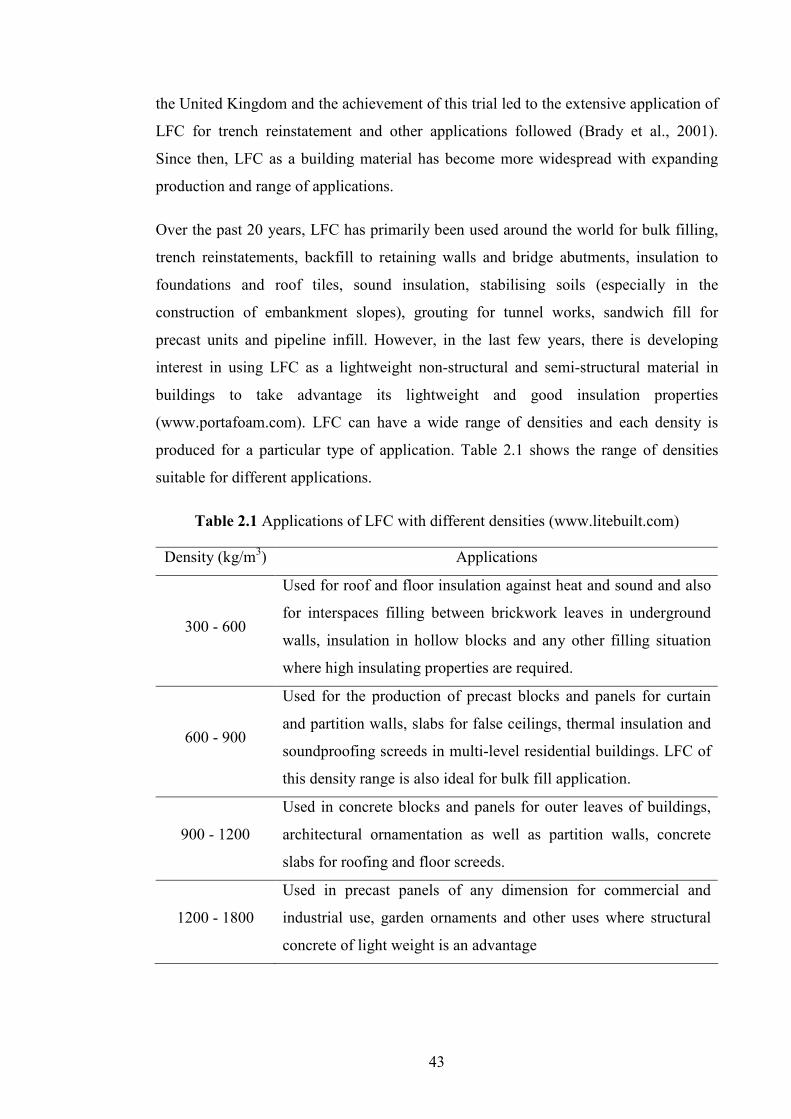
(www.portafoam.com). LFC can have a wide range of densities and each density is
produced for a particular type of application. Table 2.1 shows the range of densities
suitable for different applications.
Table 2.1 Applications of LFC with different densities (www.litebuilt.com)
Density (kg/m3) Applications
300 - 600
Used for roof and floor insulation against heat and sound and also
for interspaces filling between brickwork leaves in underground
walls, insulation in hollow blocks and any other filling situation
where high insulating properties are required.
600 - 900
Used for the production of precast blocks and panels for curtain
and partition walls, slabs for false ceilings, thermal insulation and
soundproofing screeds in multi-level residential buildings. LFC of
this density range is also ideal for bulk fill application.
900 - 1200
Used in concrete blocks and panels for outer leaves of buildings,
architectural ornamentation as well as partition walls, concrete
slabs for roofing and floor screeds.
1200 - 1800
Used in precast panels of any dimension for commercial and
industrial use, garden ornaments and other uses where structural
concrete of light weight is an advantage

44
2.1.1 Constituents material of LFC
LFC with low density, i.e. having a dry density of up to about 600 kg/m3, is frequently
formed from cement (to which other binders could be added), water and stable foam
whilst denser LFC will incorporate fine sand in the mix. The requirements of each
constituent of LFC are explained below:
2.1.1.1 Cement
Portland cement SEM1 is typically used as the main binder for LFC. Additionally,
rapid hardening Portland cement (Kearsley and Wainwright, 2001), calcium
sulfoaluminate and high alumina cement (Turner, 2001) have also been used to reduce
the setting time and to obtain better early strength of LFC. There was also an attempt to
decrease the cost of production by using fly ash (Kearsley and Wainwright, 2001) as
cement replacement to enhance consistency of the mix and to reduce heat of hydration
while contributing for long term strength. The effect of using fly ash as cement
replacement on compressive strength of LFC will be further discussed in Section 2.2.3.
2.1.1.2 Fillers (sand)
Sach and Seifert (1999) suggested that only fine sands having particle sizes up to about
4mm and with an even distribution of sizes should be used for LFC. This is primarily
because coarser aggregate might lead to collapse of the foam during the mixing
process. Coarse pulverised fuel ash (PFA) also can be used as a partial or total
replacement for sand to make LFC with a dry density below about 1400 kg/m3.
2.1.1.3 Water
The amount of water to be added to the mix depends on the composition of the mix
design. Generally for lighter densities, when the amount of foam is increased, the
amount of water can be decreased. The water-cement ratio must be kept as low as
possible in order to avoid unnecessary shrinkage in the moulds. However, if the amount
of water added to cement and sand is too low, the necessary moisture to make a
workable mix will have to be extracted from the foam after it is added, thereby
destroying some of the foam in the mix. The range of water-cement ratio used in LFC is
between 0.4 to 1.25 (Kearsley, 1996), the appropriate value will be depending on the

45
amount of cement in the mix, use of chemical admixtures and consistence requirement.
Plasticizers are not normally necessary to make LFC because of LFC has intrinsic high
workability.
2.1.1.4 Surfactants (foaming agent)
There is an extensive choice of surfactants (foaming agent) available in the market.
Generally two types of surfactants can be used to produce foam: protein and synthetic
based surfactants. Protein based surfactants are produced from refined animal products
such as hoof, horn and skin whilst synthetic based surfactants are produced using man
made chemicals such as the ones used in shampoos, soap powders and soaps (Md
Azree, 2004). The surfactant solution typically consists of one part of surfactant and
between 5 and 40 parts of water but the optimum value is a function of the type of
surfactant and the technique of production. It is very important to store all surfactants
accordingly because they are inclined to deterioration at low temperatures.
According to McGovern (2000), foams formed from protein based surfactants have
smaller bubble size, are more stable and have a stronger closed bubble structure
compared to the foam produced using synthetic surfactants. Therefore, protein based
surfactants would be best suited for the production of LFC of comparatively high
density and high strength.The stability of foam is a function of its density and the type
of surfactant. The foam has to endure its inclusion into the mortar mix and the chemical
environment of the concrete until it has attained a reasonable set. A number of external
environmental factors can exert influence on the stability of the foam such as vibration,
evaporation, wind and temperature. Some or all of these may be present on a site and
may lead to the breakdown in the foam structure.
Currently two methods can be used to produce LFC, either by pre-foaming method or
mixed foaming method. Pre-foaming involves preparation of the base mix and the
stable foam individually and then is added together. In the mixed foaming method, the
foaming agent is mixed together with the base matrix. The properties of LFC are
significantly reliant upon the quality of the foam; therefore, the foam should be firm
and stable so that it resists the pressure of the mortar until the cement takes its initial set
to allow a strong skeleton of concrete to be built up around the void filled with air
(Koudriashoff, 1949).
46
2.1.2 Design procedure of LFC
At the moment, there is no standard method for designing LFC mix. For normal weight
concrete, the user would signify a certain compressive strength and the water-cement
ratio would be adjusted to meet the requirement. As far as LFC is concerned, not only
the strength is specified, but also the density. Since the compressive strength of LFC is
a function of density, the density can be used to modify the strength but this does not
give any indication of the water requirement in the mix. It is not an easy task to achieve
an accurate measurement of the density of LFC on site because of the hardened density
of LFC depends on the saturation intensity in its pores.
According to Jones and McCarthy (2005), it is difficult to achieve the design density of
LFC because it has a tendency to lose between 50 and 200 kg/m3 of the total mix water
because it depends on the concrete fresh density, early curing regime and exposure
conditions.
2.2 RELEVA�T STUDIES O� PROPERTIES OF LFC
There is a lack of published information on LFC. Among the LFC related literature
collected by the author so far (around 60 in total), majority of these were published
within the last 10 years and most of these previous studies on LFC were aimed at
characterizing the ambient temperature properties of LFC. This section will review
previous studies on properties of hardened LFC, including physical properties (density,
air-void system and porosity), mechanical properties (compressive strength, tensile
strength and modulus of elasticity), thermal properties and fire resistance performance.
2.2.1 Density of LFC
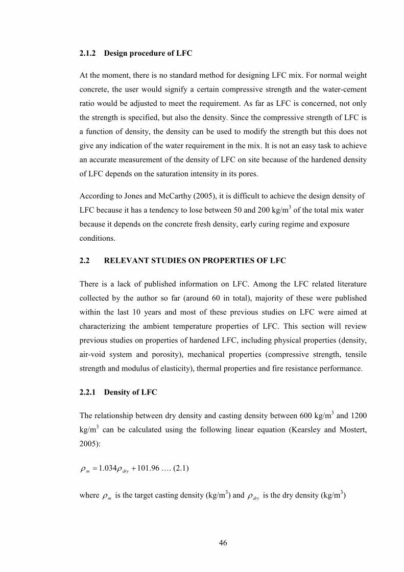
The relationship between dry density and casting density between 600 kg/m3 and 1200
kg/m3 can be calculated using the following linear equation (Kearsley and Mostert,
2005):
96.101034.1 += drym ρρ …. (2.1)
where mρ is the target casting density (kg/m3) and dryρ is the dry density (kg/m3)

47
2.2.2 Air-void system and porosity of LFC
As will be explained in sections 3.4.2, 3.4.3 and 5.2, porosity and the pore structure will
have significant effects on thermal conductivity and mechanical properties of LFC.
High porosity is highly detrimental to the strength of LFC, particularly if the pores are
of large diameter. Large pores also result in high thermal conductivity. As a cement-
based material, LFC consists of gel-pores (dimensions from 0.0005µm up to 0.01µm),
capillary-pores (0.01µm to 10µm) and air-pores (air entrained and entrapped pores)
(Visagie and Kearsely, 2002). The gel-pores occupy between 40 to 55% of total pore
volume but they are not active in permeating water through cement paste and they do
not influence the strength (Brandt, 1995). However, the water in the gel-pores is
physically bonded to cement and directly controls shrinkage and creep properties of
LFC.
Air-pores in hardened LFC can be entrained or entrapped. Entrapped air-pores occur
inadvertently during the mixing and placing of concrete. As LFC is a self-flowing and
self-compacting concrete and exclusive of any coarse aggregate, the possibility of
entrapped air is insignificant. In contrast, entrained air-pores are introduced
intentionally during production of LFC by using an air-entraining chemical admixture
(surfactants). Entrained air-pores are discrete and individual bubbles of spherical shape.
They are uniformly distributed throughout the cement paste and are not interconnected
with each other and therefore do not affect the permeability of LFC (Kalliopi, 2006).
The total volume of capillary-pores and air-pores affects the strength of LFC.
Kearsley and Wainwright (2001) carried out research to investigate the relationship
between porosity and dry density of LFC. In this study, they utilized a large amount of
both classified and unclassified fly ash (pulverised and pozz-fill) as a cement
replacement up to 75% by weight. Figure 2.1 shows the relationship between porosity
and dry density of LFC obtained from their research. It can be seen from Figure 2.1 that
there is a strong relationship between porosity and dry density of LFC. They found that
the porosity of LFC is the combination of entrained air-pores and the pores within the
paste and the porosity was found to be dependant primarily on dry density of LFC and

48
not on fly ash type and content. Kearsley and Wainwright proposed an equation to link
the porosity and dry density of LFC (based on Figure 2.1) as follows:
85.018700 −= dryρε ……(2.2)
where ε is the porosity (%) and dryρ is the dry density (kg/m3)
Figure 2.1 Porosity of LFC as a function of dry density (Kearsley and
Wainwright, 2001)
Nambiar and Ramamurthy (2007) performed a study to distinguish the air-pore
structure of LFC by identifying a few parameters that influence the density and strength
of LFC. They used a camera connected to an optical microscope and computer with
image analysis software to develop a quantification technique for these parameters. The
LFC mixes used in their investigation included cement-sand and cement-fly ash mixes
with a filler-cement ratio of 2 and varying foam volume (10% to 50%). The dimensions
of the specimens for image analysis were 50 × 50 × 25 mm. Upon completing the
image processing and air pore identification, the total area, perimeter, equivalent
diameter of every defined area (air pore) in the images were analysed to obtain the
percentage of pores, air-pore size distribution, shape of the pores in terms of shape
factor and spacing factor for each mixes. Figures 2.2 and 2.3 show typical binary
images for cement-sand mix and cement-fly ash mix respectively obtained from their
research. It can be seen that the use of fly ash as a filler in LFC mix helped in achieving
more uniform distribution of air voids than fine sand. Fly ash, being finer, helped to

49
achieve uniform distribution of air-pores by providing a well and uniform coating on
each bubble and thereby preventing it from merging and overlapping. They also
concluded that the air-pore shape had no influence on the properties of LFC as all air
pores were of roughly the same shape and independent of foam volume.
Figure 2.2 Typical binary images for cement-sand mixes (Nambiar and
Ramamurthy, 2007)
Figure 2.3 Typical binary images for cement-fly ash mixes (Nambiar and
Ramamurthy, 2007)
50
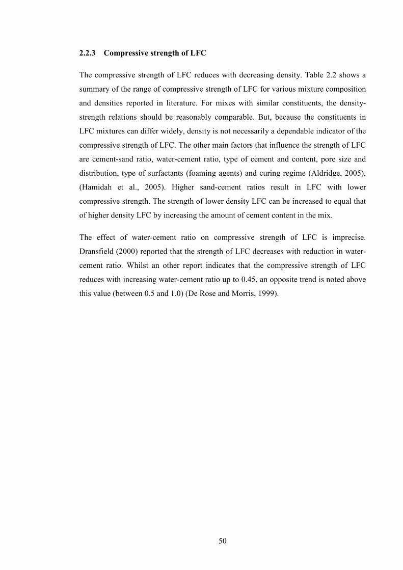
2.2.3 Compressive strength of LFC
The compressive strength of LFC reduces with decreasing density. Table 2.2 shows a
summary of the range of compressive strength of LFC for various mixture composition
and densities reported in literature. For mixes with similar constituents, the density-
strength relations should be reasonably comparable. But, because the constituents in
LFC mixtures can differ widely, density is not necessarily a dependable indicator of the
compressive strength of LFC. The other main factors that influence the strength of LFC
are cement-sand ratio, water-cement ratio, type of cement and content, pore size and
distribution, type of surfactants (foaming agents) and curing regime (Aldridge, 2005),
(Hamidah et al., 2005). Higher sand-cement ratios result in LFC with lower
compressive strength. The strength of lower density LFC can be increased to equal that
of higher density LFC by increasing the amount of cement content in the mix.
The effect of water-cement ratio on compressive strength of LFC is imprecise.
Dransfield (2000) reported that the strength of LFC decreases with reduction in water-
cement ratio. Whilst an other report indicates that the compressive strength of LFC
reduces with increasing water-cement ratio up to 0.45, an opposite trend is noted above
this value (between 0.5 and 1.0) (De Rose and Morris, 1999).

51
Table 2.2 A review of LFC mixes, compressive strengths and density ranges
(Ramamurthy et al., 2009)
Ratios
Authors
Proportion of
cement (kg/m3)
or composition S/C W/C F/C
Density
range
kg/m3
Compressive
strength
(28 days)
N/mm2
Van Deijk
(1991)
Cement-sand/
fly ash - - - 280-1200
0.6 -10.0
(91 days)
270–398 1.23-
2.5
0.61-
0.82 -
982-1185
(DD) 1.0-6.0 Durack and
Weiqing
(1998) 137-380 - 0.48-
0.70
1.48-
2.50
541-1003
(DD)
3.0-15.0
(77 days)
Kearsley and
Wainwright
(2001)
Cement-fly ash
replacement
193-577
- 0.6-
1.17 - 1000-1500 2.0-18.0
500 1.5-
2.3 0.3 - 1400-1800 10.0-26.0 Jones and
McCarthy
(2005) 500 - 0.65-
0.83
1.15-
1.77 1400-1800 20.0-43.0
Cement-sand
mix (coarse) 1.0-7.0
Cement-sand
mix (fine)
800-1350
(DD) 2.0-11.0
Nambiar and
Ramamurthy
(2006) Cement-sand-
fly ash mix
With filler-cement
ratio varied from 1 to
3 and fly ash
replacement for sand
varied from 0% to
100%
650-1200
(DD) 4.0-19.0
* S/C: sand–cement ratio; F/C: fly ash–cement ratio; W/C: water–cement ratio; DD: dry density
When cement is combined with silica fume (Kearsley, 1996) and fly ash (De Rose and
Morris, 1999), higher compressive strength is achieved in the long term, owing to their
pozzolanic reaction and filler characteristics, with a more marked effect at high LFC
densities. Kearsley and Wainwright (2001) carried out a study on the effect of replacing
large volumes of cement (up to 75% by weight) by both classified and unclassified fly
ash on strength of LFC. They found that up to 67% of the cement could be replaced
with ungraded and graded fly ash without any significant reduction in compressive

52
strength. The results signify that the compressive strength of LFC is principally a
function of dry density, and LFC mixes with high fly ash content needed a longer time
to reach their maximum strength which was observed to be higher than that attained
using only cement.
In terms of the influence of fillers on strength of LFC, better strength is obtained when
finer sand is used. For a given density, the mix with fine sand results in higher strength
than the mix with coarse sand and the variation is higher at higher density. This higher
strength-density ratio is credited to the moderately uniform distribution of pore in LFC
with fine sand, while the pores were larger and irregular for mixes with coarse sand
(Nambiar and Ramamurthy, 2006). Similar behaviour was observed when sand was
replaced by fine fly ash.
Jones and McCarthy (2005) performed an extensive experimental exploration into the
effect of utilization of unprocessed, run-of-station, low-lime fly ash in LFC, as a
substitution for sand on the rheological, strength development and
permeation/durability properties for LFC with plastic densities ranging between 1000
and 1400 kg/m3. They found that the use of fly ash in LFC considerably benefited the
compressive strength growth, predominantly after 28 days. At a given age, the fly ash
coarse concretes were up to 6 times stronger than those of equivalent sand concretes.
The enhancement of strength with fly ash as filler is not pronounced at lower density
range (higher percentage of foam volume) especially at earlier ages. This is due to the
fact that at lower density range, the foam volume controls the strength rather than the
material properties (Nambiar and Ramamurthy, 2006). The utilization of lime,
demolition fines, recycled glass as fine aggregate has slight or no effect on compressive
strength of LFC, while some decrease in strength was reported when crumb rubber,
used foundry sand, china clay sand and quarry fines were used (De Rose and Morris,
1999), (Jones et al., 2005).
The compressive strength of LFC decreases with an increase in pore diameter for dry
density of LFC between 500 and 1000 kg/m3. Nevertheless for densities higher than
1000 kg/m3, as the air-pores are far apart to have an influence on the compressive
strength, the composition of the paste determines the compressive strength (Visagie and
Kearsely, 2002). The type of surfactant (foaming agent) also has major effect on the

53
compressive strength of LFC. An increased of strength up to 70% was found with the
used of protein based foaming agent rather than synthetic foaming agent (Dransfield,
2000).
In terms of curing regime, autoclaving increases the compressive strength. Hamidah et
al. (2005) carried out an investigation to produce cost-effective mix for LFC by
optimising the amount of sand in LFC mix by using different sand-cement ratio and
curing conditions. In this study, a series of LFC of four different densities ranging from
1300 to 1600 kg/m3 was fabricated using the appropriate mix proportions and a series
of sand-cement ratios varying from zero to 2.0 for each series of density was attempted.
Hamidah et al. found that water cured samples of LFC attained higher strength than
those cured in air. For cement based material, the presence of water could promote the
hydration process of cement for strength development, nevertheless the existence of
foam in cement would delay the hydration and thus it is expected that LFC could only
achieve maximum strength at later ages compared to that of normal weight concrete.
Kearsley and Mostert (2005) appears to be the only ones to have carried out an
investigation to look into the effect of cement composition on the compressive strength
of LFC exposed to high temperatures. From their background study, they found that
Portland cement SEM1 was not suitable to fabricate LFC based firewalls for
temperatures above 400°C. Above this temperature point, the calcium hydroxide in
Portland cement SEM1 dehydrates forming calcium oxide. When calcium oxide reacts
with water, damage will happen in the form of swelling and cracking. Montgomery
(2003) used calcium aluminate cements to manufacture concrete that needs to withstand
temperatures in excess of 300-400°C. The use of aluminate cement was found to
increase the service temperature limit and enhance the ability of the material to
withstand high temperatures which is due to the present of compounds with lower
melting points in calcium aluminate. Therefore high alumina cement was used in the
investigation carried out by Kearsley and Mostert (2005). Dolomite sand and fly ash
were used in the mix to determine the effect of filler type on the properties of LFC.
Table 2.3 shows the chemical composition of the materials used in their study where
three types of cement composition were used, with increasing aluminate and decreasing
calcium contents. From the experimental results, they found that compressive strength
of LFC containing dolomite was noticeably reduced upon exposure to high

54
temperatures as shown in Figure 2.4. From Figure 2.4, it can be seen that the
compressive strength of LFC containing dolomite is significantly lower than the
strength of samples containing fly ash. The compressive strength of samples containing
fly ash mixed with the cement with lower aluminate content (cement Type 2 in Table
2.3) increased significantly at high temperatures up to 800°C (refer Figure 2.5). The
increase in strength can be attributed to the high strength ceramic bonds that developed
as a result of thermo-chemical reactions at high temperatures. Figure 2.6 demonstrates
the compressive strength of LFC containing Cement Type 3. The variation of
compressive strength as a function of testing density shown in Figure 2.6 was found to
be the same as that observed in LFC samples containing Cement Type 2 (Figure 2.5).
Nevertheless the variation in compressive strength of LFC after heating seems to be
less for the LFC containing cement with higher alumina content. LFC samples
containing Cement Type 3 seem to result in slightly higher compressive strengths.
Table 2.3 Chemical composition of cement used in Kearsley and Mostert study
Oxides Portland
Cement
Fly Ash
(%)
Cement
Type 1 (%)
Cement
Type 2 (%)
Cement
Type 3 (%)
CaO 65.0 0.05 ≤ 39.8 ≤ 39.5 28.5 - 30.5
SiO2 20.7 39.5 ≤ 6.0 ≤ 6.0 0.2 - 0.6
Al2O3 4.47 57.8 ≥ 37.0 ≥ 50.0 68.7 - 70.5
Fe2O3 2.87 0.79 ≤ 18.5 ≤ 3.0 0.1 - 0..3
TiO2 0.43 0.21 < 4.0 < 4.0 < 0.4
Na2O 0.09 0.05
K2O 0.04 0.29 < 0.4 < 4.0 < 0.5
MgO 2.13 0.31 < 1.5 < 1.0 < 0.5
SO3 2.89 280 ppm < 0.4 < 0.4 < 0.3
Al2O3/ CaO
ratio 0.07 - ±0.9 ±1.3 ±2.4
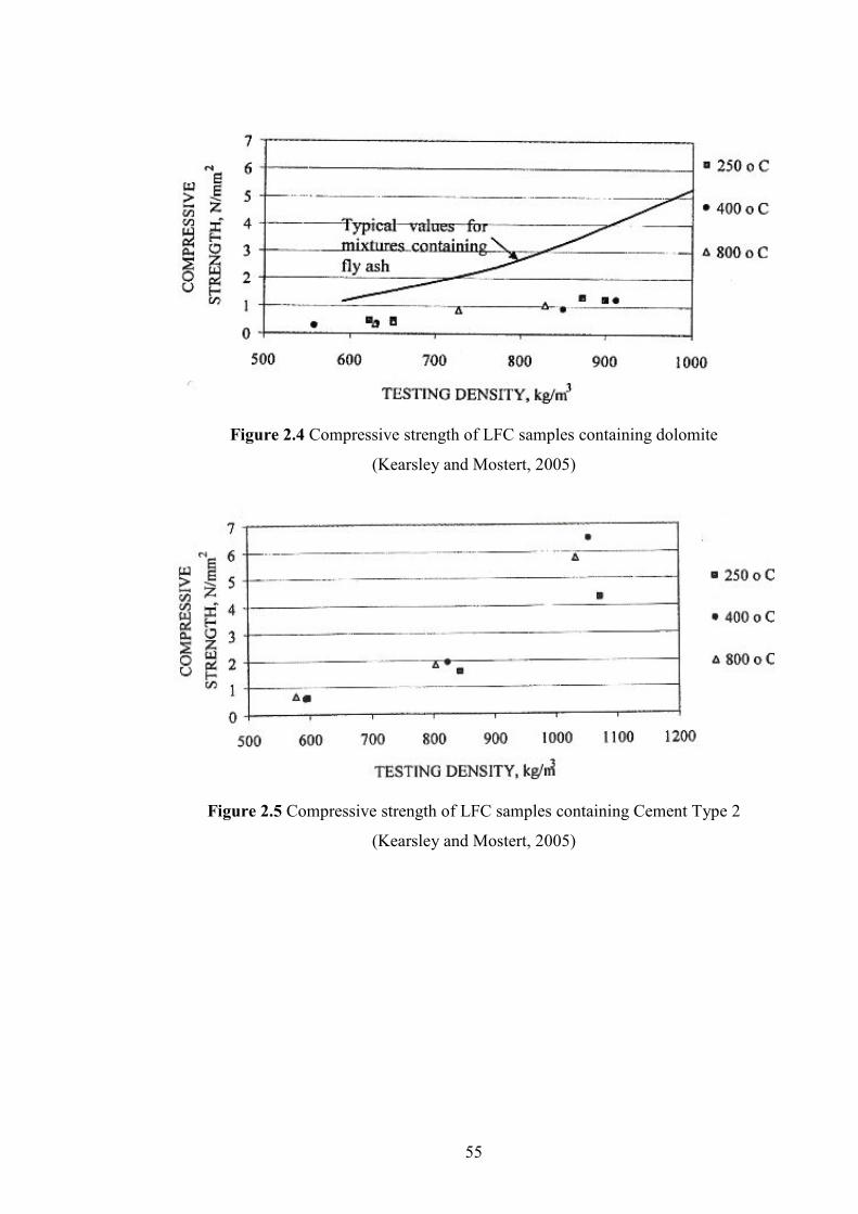
55
Figure 2.4 Compressive strength of LFC samples containing dolomite
(Kearsley and Mostert, 2005)
Figure 2.5 Compressive strength of LFC samples containing Cement Type 2
(Kearsley and Mostert, 2005)

56
Figure 2.6 Compressive strength of LFC samples containing Cement Type 3 (Kearsley
and Mostert, 2005)
Table 2.4 summarizes the effect of different parameters on compressive strength of
LFC.
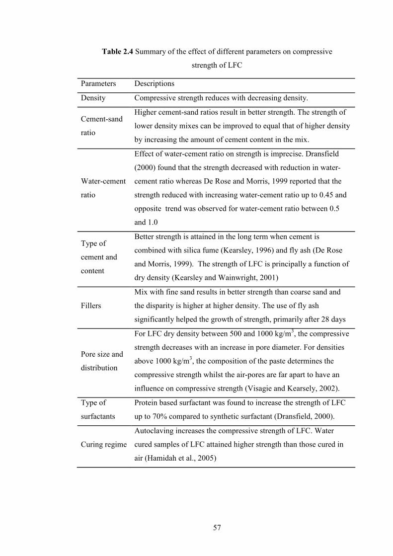
57
Table 2.4 Summary of the effect of different parameters on compressive
strength of LFC
Parameters Descriptions
Density Compressive strength reduces with decreasing density.
Cement-sand
ratio
Higher cement-sand ratios result in better strength. The strength of
lower density mixes can be improved to equal that of higher density
by increasing the amount of cement content in the mix.
Water-cement
ratio
Effect of water-cement ratio on strength is imprecise. Dransfield
(2000) found that the strength decreased with reduction in water-
cement ratio whereas De Rose and Morris, 1999 reported that the
strength reduced with increasing water-cement ratio up to 0.45 and
opposite trend was observed for water-cement ratio between 0.5
and 1.0
Type of
cement and
content
Better strength is attained in the long term when cement is
combined with silica fume (Kearsley, 1996) and fly ash (De Rose
and Morris, 1999). The strength of LFC is principally a function of
dry density (Kearsley and Wainwright, 2001)
Fillers
Mix with fine sand results in better strength than coarse sand and
the disparity is higher at higher density. The use of fly ash
significantly helped the growth of strength, primarily after 28 days
Pore size and
distribution
For LFC dry density between 500 and 1000 kg/m3, the compressive
strength decreases with an increase in pore diameter. For densities
above 1000 kg/m3, the composition of the paste determines the
compressive strength whilst the air-pores are far apart to have an
influence on compressive strength (Visagie and Kearsely, 2002).
Type of
surfactants
Protein based surfactant was found to increase the strength of LFC
up to 70% compared to synthetic surfactant (Dransfield, 2000).
Curing regime
Autoclaving increases the compressive strength of LFC. Water
cured samples of LFC attained higher strength than those cured in
air (Hamidah et al., 2005)

58
2.2.4 Flexural and tensile strength of LFC
The ratio of flexural strength to compressive strength of LFC is in the range of 0.06–
0.10 and this ratio was also found to reduce with increasing water-cement ratios and
decreasing densities (Van Deijk, 1991). The splitting tensile strengths of LFC mixes are
higher for mixes with sand than those with fly ash. This is attributed to the improved
shear capacity between sand particles and the paste phase (Jones and McCarthy, 2005).
The introduction of polypropylene fibers in LFC mix has been reported to improve the
tensile and flexural strength of LFC, provided this does not affect the fresh concrete
behavior and self-compaction (Kearsely and Mostert, 1997).
2.2.5 Modulus of elasticity of LFC
As a porous material, the static modulus of elasticity of LFC is expected to be
considerably lower than that of normal weight concrete for dry densities between 500
and 1500 kg/m3 with values typically varying from 1.0 to 8.0 kN/mm2, respectively
(Jones and McCarthy, 2005). LFC mix containing fly ash as fine aggregate is reported
to show lower modulus of elasticity value than that of LFC with sand. Jones and
McCarthy (2005) reported that the utilization of polypropylene fibers in LFC mix could
enhance the value of modulus of elasticity of LFC between two and four times. They
proposed two relationships to predict the modulus of elasticity of LFC as follows:
Sand as fine aggregate 18.142.0 cc fE = …. (2.3)
Fly ash as fine aggregate 67.099.0 cc fE = …. (2.4)
where cE is the modulus of elasticity (kN/mm2) and fc is the compressive strength
(N/mm2).
Figure 2.7 shows a plot of modulus of elasticity against compressive strength based on
Equation 2.3 and Equation 2.4. From Figure 2.7, it can be seen that for the same
compressive strength (fc), sand as aggregate gives higher modulus of elasticity values
compared to fly ash aggregate. This difference is attributed to the high amount of fine
aggregate in sand mix compared to fly ash mix, which contains completely paste with
no aggregate (Jones, 2001).

59
0
5
10
15
20
25
0 5 10 15 20 25 30 35Compressive Strength (�/mm
2)
Mo
du
lus
of
ela
stic
ity
(k
�/m
m2)
Sand as fine aggregate
Fly ash as fine aggregate
Figure 2.7 Relationship between modulus of elasticity and compressive
strength of LFC
2.2.6 Thermal properties of LFC
Thermal properties are required in two design considerations: to provide thermal
insulation at ambient temperature and to provide fire resistance. There is some data of
LFC thermal properties at ambient temperature but little information is available for
LFC thermal properties at elevated temperatures. One of the important objectives of
this research is to obtain thermal properties of LFC at elevated temperatures for
assessment of fire resistance.
2.2.6.1 Ambient temperature thermal properties
The cellular microstructure of LFC provides it with low thermal conductivity.
According to BCA (1994) and Jones and McCarthy (2005), the thermal conductivity of
LFC typically is 5 to 30% of that of normal weight concrete and range from between
0.1 and 0.7 W/mK for dry density values of 600 to 1600 kg/m3 respectively. As pointed
out by Kessler (1998), in practical terms normal weight concrete would have to be 5
times thicker than LFC ones to achieve similar thermal insulation. The thermal
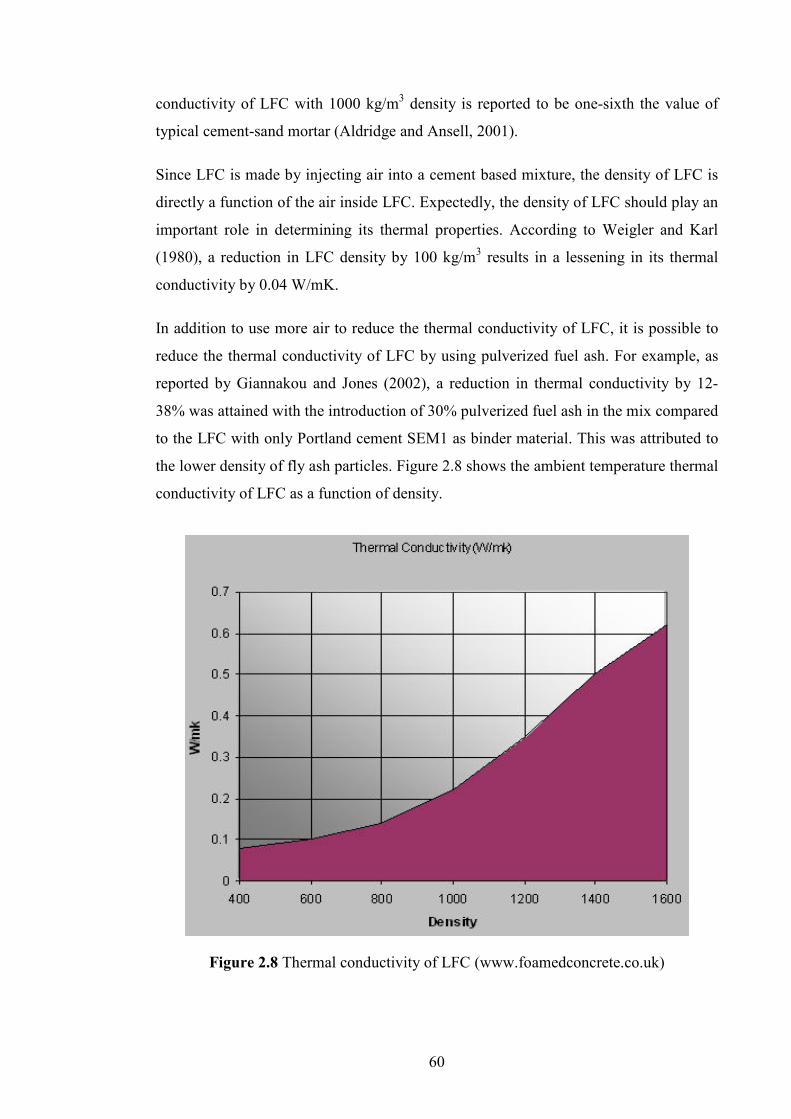
60
conductivity of LFC with 1000 kg/m3 density is reported to be one-sixth the value of
typical cement-sand mortar (Aldridge and Ansell, 2001).
Since LFC is made by injecting air into a cement based mixture, the density of LFC is
directly a function of the air inside LFC. Expectedly, the density of LFC should play an
important role in determining its thermal properties. According to Weigler and Karl
(1980), a reduction in LFC density by 100 kg/m3 results in a lessening in its thermal
conductivity by 0.04 W/mK.
In addition to use more air to reduce the thermal conductivity of LFC, it is possible to
reduce the thermal conductivity of LFC by using pulverized fuel ash. For example, as
reported by Giannakou and Jones (2002), a reduction in thermal conductivity by 12-
38% was attained with the introduction of 30% pulverized fuel ash in the mix compared
to the LFC with only Portland cement SEM1 as binder material. This was attributed to
the lower density of fly ash particles. Figure 2.8 shows the ambient temperature thermal
conductivity of LFC as a function of density.
Figure 2.8 Thermal conductivity of LFC (www.foamedconcrete.co.uk)

61
2.2.6.2 Fire resistance and elevated temperature thermal properties
To evaluate fire resistance of a construction element, it is necessary to carry out heat
transfer analysis to obtain temperature information and structural assessment.
Temperature dependent thermal and mechanical properties are required. Compared to
ambient temperature studies on LFC, there is little quantitative information available on
elevated temperature thermal and mechanical properties of LFC. A major contribution
of this study will be to help fill this significant knowledge gap.
According to Kessler (1998), the fire resistance of LFC is excellent; at low
temperatures it is better than normal weight concrete in terms of the proportional loss in
strength. But when exposed to high temperatures, it suffers from excessive drying
shrinkage (Sach and Seifert, 1999). Study carried out by Kearsley and Mostert (2005)
on the effect of cement composition on the properties of LFC exposed to high
temperature indicated that LFC containing hydraulic cement with an Al2O3/CaO ratio
higher than two could withstand temperatures as high as 1450°C without showing any
sign of damage. According to Jones and McCarthy (2005), LFC has been found to be
incombustible, and in a test on LFC concrete slabs with 100mm thickness, standard fire
resistance of 2 ½ hours and 3 ¾ hours for 1250 kg/m3 and 930 kg/m3 oven dry densities
respectively was established based on thermal insulation.
2.3 LIMITATIO� I� PREVIOUS STUDIES O� LFC PROPERTIES
The literature review presented in Section 2.2 clearly indicates that most of the
investigations on LFC so far have focused on its ambient temperature properties only.
Among these, the majority are about mechanical properties of LFC with only a very
few on its thermal properties. Quantitative information on fire resistance performance is
extremely sparse.
Nevertheless the reviewed literature does give some useful data of LFC mechanical and
thermal properties at ambient temperature which can be used as the basis for further
research. In particular, it is important to identify the most important parameters that
influence the mechanical and thermal properties of cement-based LFC at elevated
temperatures so that appropriate quantification models may be developed. Section 2.4
will further discuss the influential parameters.

62
2.4 PROPERTIES OF CEME�T-BASED MATERIAL AT ELEVATED
TEMPERATURES
This section describes the thermal and mechanical properties of cement-based material
at high temperatures. It will briefly explain the reasons for the changes in LFC
properties during heating so as to provide references for further understanding of the
changes. Chapter 3 and Chapter 6 will provide detailed explanations and development
of thermal properties and mechanical properties models correspondingly.
2.4.1 Thermal properties of cement-based material
As mentioned earlier, LFC is a composite material made from a combination of filler
(sand), cement binder and water. After mixing, the cement hydrates and hardens into a
stone like material. Theoretically, combined mass and heat transfer should be carried
out to obtain temperatures in LFC construction. However, modelling mass transfer
(water movement) is complex. A common approximation is to conduct heat transfer
only, but modifying the material thermal properties to reflect the effects of water
movement. For heat transfer analysis, data on thermal conductivity, specific heat and
density should be provided.
When cement-based material like LFC is exposed to high temperatures, the free water
in the pores and some chemically bonded water in the hydrated cement paste are
released, consuming a large amount of energy, just as happens in normal weight
concrete. A few authors have described the reactions that take place in cement-based
material at high temperatures. Vaporization of the free water takes place at around
100°C (Noumowe, 1995). It is generally considered that the evaporable water is
completely eliminated at 120°C. Then between 180 to 300°C, loss of the chemically
bond water happens through decomposition of the C-S-H and carboaluminate hydrates
(Khoury, 1992). The high temperatures in the range of 400 to 600°C may then stimulate
a series of reactions in the hardened LFC paste. These reactions originate with the
complete desiccation of the pore system, followed by decomposition of the hydration
products and the destruction of C-S-H gels (Rostasy, 1995). The conversion of calcium
hydroxide into lime and water vapour during heating may lead to serious damage due to
lime expansion (Lin et al., 1996). These changes will affect the thermal properties of
LFC.

63
2.4.1.1 Thermal conductivity
Given that LFC is a porous material, its effective thermal conductivity will be affected
by the air voids inside, and heat transfer through LFC should consider all three modes
of heat transfer: conduction through the solid, and convection and radiation through the
pores. Therefore the effective thermal conductivity of LFC should include these effects.
Within each air-void, heat conduction will dominate at relatively low temperatures. At
high temperatures, radiation will play a much more important role because the radiation
coefficient is related to temperature raised to power three. The effective thermal
conductivity of LFC at elevated temperatures depends not only on the thermal
conductivities of the cement and the air, but also radiation effect inside the air voids.
2.4.1.2 Specific heat
The specific heat is the amount of heat energy per unit mass required to change the
temperature of the material by one degree. Compared to thermal conductivity, this
thermal property does not vary much with temperature. It has been found that filler
type, mix proportion or age do not have great effect on the specific heat of ordinary
cement-based material (Carman and Nelson, 1921). The main factor affecting the
specific heat of LFC is the moisture content at the time of heating as water has
relatively high specific heat. The specific heat of LFC consists of the base value of the
dry components and the heat consumed heat due to water evaporation. During water
evaporation, most of the heat supplied to the concrete is used for the removal of water
and only a small amount is available for raising the temperature of the material. As a
consequence, the specific heat increases considerably in these temperature intervals.
2.4.1.3 Density
The density of cement-based material like LFC is affected by the evaporation of water
and reduces with increasing temperature.
2.4.2 Mechanical properties of cement-based material
Mechanical properties of concrete due to exposure to elevated temperatures have been
studied since a long time ago. Table 2.5 provides a summary of investigations on
normal weight concrete at elevated temperatures. Influence of these earlier studies have

64
provided data which formed the technical basis for the provisions and recommendations
for determining concrete mechanical properties exposed to elevated temperatures in
many existing codes.
Table 2.5 Summary of studies on normal weight concrete at elevated temperatures
Researchers Properties Descriptions
Li and Purkiss
(2005)
Compressive strength,
modulus of elasticity,
strain at peak
compressive stress
Performed a transient test on mechanical
properties of concrete at high
temperatures
Hertz (2005) Compressive strength
Study on compressive strength of
concrete that allowed for different types
of aggregate at high temperatures
Lu (1989) Modulus of elasticity
Investigation of fire response of
reinforced concrete beams based on
unstressed test procedure
Li and Guo
(1993)
Modulus of elasticity,
flexural tensile strength
Experimental investigation on strength
and deformation of concrete under high
temperature
Khennane and
Baker (1993)
Modulus of elasticity,
Strain at peak
compressive stress
Investigation on concrete behavior
under variable temperature and stress at
high temperatures
Anderberg and
Thelandersson
(1976)
Strain at peak
compressive stress,
stress-strain relationship,
flexural tensile strength
Study on mechanical properties of
concrete based on transient tests at high
temperatures
Bazant and
Chern (1987)
Strain at peak
compressive stress
Investigation of strain behavior of
unstressed concrete at high temperatures
Lie and Lin
model (1985) Stress-strain relationship
Study on stress-strain relationship of
concrete exposed to high temperatures
Terro (1998) Flexural tensile strength
Carried out numerical modeling of the
behavior of concrete structures under
fire condition

65
There is no such extensive study of mechanical properties of LFC at elevated
temperatures. Therefore Chapter 6 will assess the applicability of the different models
suggested by various researchers presented in Table 2.5 for normal weight concrete to
LFC.
Lin et al. (1996) conducted studies to investigate the microstructure of concrete
exposed to elevated temperatures in both actual fire and laboratory conditions with the
assistance of Scanning-Electron-Microscopy (SEM) and stereo microscopy. They found
that the absorption of moisture from the surrounding medium provides a mechanism for
the rehydration of calcium oxide and unhydrated cement grains that refilled the void
spaces. They observed that long irregular fibers of C-S-H gel combined with ettringite
and C-H crystals and formed as a result of rehydration.
In a study carried out by Schneider and Herbst (1989), chemical reactions and the
behavior of calcium hydroxide, calcium carbonate, calcium silicate hydrate, non-
evaporable water and micropores under various temperatures was examined. They
found that the major increase of concrete permeability and porosity at high temperature
was primarily produced by arising microcracks and by changes of material inner
structure, as well as by crack opening due to high gas pressure values. As a result, the
permeability of concrete depends not only on temperature levels, moisture content and
gas pressure but also upon the degree of crack development.
It can be pointed out that the degradation mechanisms of cement-based material like
LFC upon exposure to elevated temperatures include chemical degradation and
mechanical deterioration where each mechanism is dominant within a specific
temperature range. Chemical degradation occurs when the chemically bound water is
released from the cement paste. The dehydration process in the cement paste becomes
significant at temperatures above about 110 °C (Khoury et al., 2002) and diminishes the
calcium silicate hydrate (C-S-H) links which provide the primary load-bearing
formation in the hydrated cement. Furthermore, due to low permeability of the cement
paste, internal water pressure built up during dehydration of the hydrated C-S-H, which
increases internal stresses and induce microcracks in the material from about 300°C,
resulting in decreased strength and stiffness of the material (Hertz, 2005), (Ai et al.,
2001). At higher temperatures around 450°C, calcium hydroxide (Ca(OH)2), which is
one of the most vital compounds in cement paste, dissociates, resulting in the shrinkage

66
of LFC (Taylor, 1992). If the hot LFC is exposed to water, as in fire fighting, CaO in
LFC turns into Ca(OH)2 to cause cracking and destruction of LFC. It is still extremely
difficult to accurately predict these mechanisms and experimental investigation remains
essential.
2.4.3 Conclusions
Sections 2.4.1 and 2.4.2 have presented some brief explanations of thermal and
mechanical properties of cement-based material at high temperatures. Cement-based
material was found to be fundamentally a complex material and its properties can
change dramatically when exposed to high temperatures thermally and mechanically.
The principal effects of high temperatures on cement-based material are loss of
compressive strength and stiffness, and increase in thermal conductivity. Though a lot
of information has been gathered on both phenomena on cement-based material, there
remains a need for more systematic studies of the effects of high temperatures on
thermal and mechanical properties of LFC at high temperatures.
For thermal properties, all the key parameters such as density, specific heat and thermal
conductivity has been identified and behaviour upon exposure to high temperatures has
been discussed in brief. Particular attention will be given on these 3 main parameters
and detailed explanations will be presented in Chapter 3 and Chapter 4.
On the other hand, for mechanical properties, the behavior of cement-based material
has been discussed in terms of chemical degradation and mechanical deterioration when
exposed to high temperatures. Summary of studies on normal weight concrete at
elevated temperatures also have been identified which will be focused to develop
conceptual models in order to establish a general methodology for use in finite element
analysis of a concrete structure. These models will be further discussed in Chapter 6 to
assess the applicability of these models to LFC.
2.5 POTE�TIAL OF LFC FOR APPLICATIO� AS COMPOSITE
STRUCTURAL LOAD-BEARI�G SYSTEM
As has become clear through this literature review, there is very little data and no
systematic study of LFC thermal and mechanical properties at ambient and elevated
temperatures. A major contribution of this research will be to fill this significant

67
knowledge gap. As part of this study investigating the use of LFC as a potential
structural load-bearing material for building applications, this research will also
investigate the performance of one type of structural element: lightweight composite
panel under compression. This section provides a brief general review of the behaviour
of this type of construction. Detailed models of calculation will be presented in
Chapter 7.
This particular type of construction has been chosen because of its low thermal
conductivity (leading to good insulation and high fire resistance) and usable amount of
compressive resistance. It is considered feasible to construct lightweight LFC panels to
be carried by manual workers on site without the use of machinery. However, since
LFC is brittle, a suitable method of using LFC in load-bearing construction would be to
use it in composite action with steel, which has high ductility. Should LFC be cast in-
situ, the thin steel sheeting can be used as formwork during construction. The need for
plywood formwork and the detailing of steel reinforcing bars is largely eliminated
which significantly reduces the construction time and cost. Furthermore, because of the
low density of LFC, the pressure on the steel sheeting during construction would be
much lower than the case with normal weight concrete, allowing thin steel sheeting to
be used.
When using thin-walled steel sheeting, the problem of local buckling under
compression (Figure 2.9) should be considered. When using normal weight concrete in
composite panel system, inward local buckling of the steel sheeting is prevented by the
concrete inside (Figure 2.10). Because of low elastic stiffness of LFC, it is necessary to
investigate whether LFC could still maintain this function.

68
Figure 2.9 Local buckling in thin-walled steel section
(a) steel section (b) composite section
Figure 2.10 Buckling modes of steel sections and composite sections (Shanmugam and
Lakshmi, 2001)
The behaviour of steel-concrete composite structural elements under compression has
been the subject of research of many researchers; majority of these researches are on
composite columns. A few research studies, e.g. Wright and Gallocher (1995) and
Wright (1998) mainly focused on composite walling. Application of the conclusions of
these studies on composite walling to equivalent LFC systems will be explained in
more detail in Chapter 7.
Central to determining the load carrying capacity of LFC composite walling system is
quantification of local buckling of the steel sheeting acting in contact with concrete. A
number of options are available and the applicability of these options to LFC panels
will be assessed in Chapter 8.

69
2.6 SUMMARY
This chapter has comprehensively summarized the existing relevant studies on
lightweight foamed concrete (LFC), including the method of production, mix design,
mechanical properties, thermal properties and fire resistance performance. Key
parameters that influence LFC thermal and mechanical parameters at ambient and
elevated temperatures were identified. At ambient temperatures, the main parameters
affecting the mechanical properties of LFC are the density, cement-sand ratio, water-
cement ratio, type of cement and content, fillers, pore size and distribution, type of
surfactants and curing regime. At high temperatures the mechanical properties of LFC
are influenced by the chemical degradation and mechanical deterioration. Conversely,
the key parameters affecting the thermal properties at ambient temperature are LFC
density, porosity (amount of air inside) and the composition of the mix whilst at high
temperatures. The important parameters are density, specific heat and thermal
conductivity which is temperature dependent and highly influenced by water content.
These key parameters will be used to guide development of experimentally based
theoretical models to quantify LFC thermal and mechanical properties at ambient and
elevated temperatures. This review has highlighted the potential application of LFC as a
structural load-bearing element in low-rise residential construction.

70
CCHHAAPPTTEERR 33
EEXXPPEERRIIMMEE��TTSS FFOORR DDEETTEERRMMII��II��GG TTHHEERRMMAALL
PPRROOPPEERRTTIIEESS OOFF LLFFCC AATT EELLEEVVAATTEEDD TTEEMMPPEERRAATTUURREESS
3.1 I�TRODUCTIO�
As outlined in the previous chapter, this research includes investigation of thermal
properties of LFC exposed to high temperatures. The thermal parameters investigated
are thermal conductivity (k), specific heat (c) and density (ρ). This research will present
experimental, analytical and numerical modelling results. This chapter will present the
experimental results and Chapter 4 will present thermal property models and their
validation using the experimental results of this chapter.
The density of LFC may be obtained by direct measurement and the results will be
presented in this chapter. The specific heat of LFC may be calculated based on those of
its constituent materials. LFC is lightweight but highly insulating. Therefore, among the
three thermal properties considered, thermal conductivity is the most important factor.
This will be further confirmed in Chapter 4 through the results of a sensitivity study in
which the sensitivity of temperatures in LFC to changes in specific heat and thermal
conductivity will be conducted. Therefore, the main emphasis of this research will be
on thermal conductivity.
The thermal conductivity of LFC may be directly measured, as will be shown in this
chapter. However, direct measurement of thermal conductivity requires expensive
equipment and becomes very difficult at high temperatures. If only using direct
measurement, it will be necessary to perform the experiments for LFC with any change
in density. Another disadvantage with direct measurement is that it does not provide
any understanding of how the material behaves. Therefore, this research has considered
an alternative. In this method, a transient heat transfer test, exposing one side of an LFC

71
slab to high temperature and the other side to ambient temperature, is carried out. With
the aid of a validated one-dimensional heat transfer analysis programme, the thermal
conductivity of the LFC is obtained through trial and error. This trial and error process
is not random and is based on theoretical consideration of thermal conductivity of LFC
as a porous material. This chapter will present the experimental results, using both the
alternative method of heating LFC slabs and the direct thermal conductivity
measurement method, the guarded hot plate test. Chapter 4 will present the basics of the
one-dimensional heat transfer programme and its validation, the thermal conductivity
model for porous material, determination of LFC thermal conductivity-temperature
relationships and comparison between these relationships with direct thermal
conductivity test results.
3.2 HEAT TRA�SFER TESTS O� LFC SLABS
3.2.1 Material constituents and design procedure of LFC
The LFC used in this study will be made from Portland cement SEM1, fine sand, water
and stable foam in which the details of the constituent materials is shown in Table 3.1.
The main objectives of this research are to determine the thermal and mechanical
properties of LFC at high temperatures therefore only a constant cement-sand ratio of
2:1 and water-cement ratio of 0.5 will be used for all batches of LFC samples made for
this research. A higher cement-sand ratio (2:1) was chosen to achieve better
compressive strength and water-cement ratio of 0.5 was found acceptable to achieve
adequate workability (Md Azree, 2004)
LFC samples of two densities of 650 and 1000 kg/m3 will be cast and tested for thermal
and mechanical properties test. The 650 kg/m3 density was selected so as to enable
comparison of thermal performance between LFC and that of other building materials
of similar density, such as gypsum board; the 1000 kg/m3 density will be used because
LFC of this density would have a useful amount of mechanical properties to make it
viable as a light load-bearing infill material, which may be combined with thin-walled
steel in lightweight composite panel construction.

72
Table 3.1 Constituent materials used to produce LFC
Constituents Type
Cement Portland cement SEM1 (BS EN 197-1, 2000)
Sand Fine sand with additional sieving to remove particles greater than
2.36 mm, to improve the LFC flow characteristics and stability. (BS
EN 12620, 2002)
Stable foam Noraite PA-1 (protein based) surfactant with weight of around 70 to
80 gram/litre produce from Portafoam TM2 System. The surfactant
solution consists of one part of surfactant to 33 parts of water.
For this research, the design method recommended by the supplier of the foam making
machine (Portafoam) from the University of Science Malaysia (www.portafoam.com)
will be followed. It has the following 4 main steps:
(i) Decide the dry density and how much foamed concrete is required.
� For example target volume of foamed concrete required = 0.04 m3
� Dry density = 700 kg/m3
� Wet density = 700 + 100 = 800 kg/m3 (based on density loss of 100 kg/m3)
(ii) Calculate the weight of raw material needed.
� Total mass of raw materials = 0.04 x 800 = 32 kg
� This is made up of cement, sand, water and stable foam.
� Assuming foam weight is 5% of total mass
� Actual mass of solids ( sand + cement + water ) = 0.95 x 32 = 30.4 kg
� Assuming a cement-sand ratio of 2.0 and water-cement 0.5, the proportion of
each material is as follows:
� Cement = 15.2 kg , Sand = 7.6 kg , Water = 7.6 kg

73
(iii) Measure and calculate the mortar slurry density and slurry volume.
� Mix and measure the mortar slurry density and calculate its volume according to
actual mix above.
� Slurry density = 2100 kg/m3 (e.g. as measured)
� slurry volume = 30.4 / 2100 = 0.01447 m3
(iv) Calculate the foam content in the mix from the foamed volume
� Foamed volume = 0.04 m3
� Foam required in mix = 0.04 – 0.01447 = 0.02553 m3
� Therefore estimated foam volume required = 25.53 litres
3.2.2 Methods of production and specimen preparation
All LFC samples were made in house. The stable foam was produced using foam
generator Portafoam TM2 System (Figure 3.1), purchased from the Malaysian
manufacturer (www.portafoam.com). This system runs from an air compressor and
consists of a main generating unit, a foaming unit, and a lance unit. The foaming agent
used was Noraite PA-1 (protein based) which is suitable for LFC densities ranging from
600 to 1600 kg/m3. Noraite PA-1 comes from natural sources and has a weight of
around 80 gram/litre and expands about 12.5 times when used with the Portafoam foam
generator. Thermocouples were positioned during casting the LFC specimens. These
thermocouples were found to be in the correct positions once the samples dried.

74
Figure 3.1 Portafoam TM2 foam generator system.
LFC was produced using a mixer by adding up the preformed foam to a base mortar
mix. Any common type of mixer (tilt drum or pan mixer used for concrete or mortar) is
suitable for LFC. The process of mixing consists of combining the cement and filler
with water and mixing it until a homogeneous base mix is accomplished. The foam
must be instantly added to the base mix and mixed until there is no physical sign of the
foam on the surface and the foam is consistently dispersed and integrated in the mix.
Figures 3.2-3.5 are provided to show how the production is carried out.
Three identical specimens were prepared for each density and were tested at 14 days
after mixing. The slab tests were conducted in an electrically heated kiln. For these
tests, LFC panels of densities 650 and 1000 kg/m3 were cast and tested. All specimens
had dimensions of 430 mm x 415 mm in plan and 150 mm in thickness. The high
temperature tests were performed for two duplicate samples of each density.
Air compressor
Holding tank
Main generating unit
Lance Unit

75
Figure 3.2 Loading of water into the mixer
Figure 3.3 Loading of fine sand and cement into the mixer

76
Figure 3.4 Adding the foam into the mortar slurry
Figure 3.5 Checking the wet density of the mix
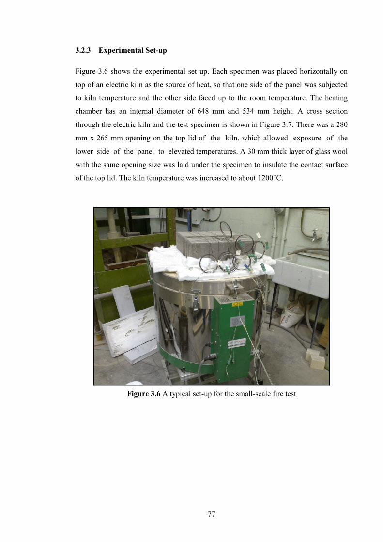
77
3.2.3 Experimental Set-up
Figure 3.6 shows the experimental set up. Each specimen was placed horizontally on
top of an electric kiln as the source of heat, so that one side of the panel was subjected
to kiln temperature and the other side faced up to the room temperature. The heating
chamber has an internal diameter of 648 mm and 534 mm height. A cross section
through the electric kiln and the test specimen is shown in Figure 3.7. There was a 280
mm x 265 mm opening on the top lid of the kiln, which allowed exposure of the
lower side of the panel to elevated temperatures. A 30 mm thick layer of glass wool
with the same opening size was laid under the specimen to insulate the contact surface
of the top lid. The kiln temperature was increased to about 1200°C.
Figure 3.6 A typical set-up for the small-scale fire test
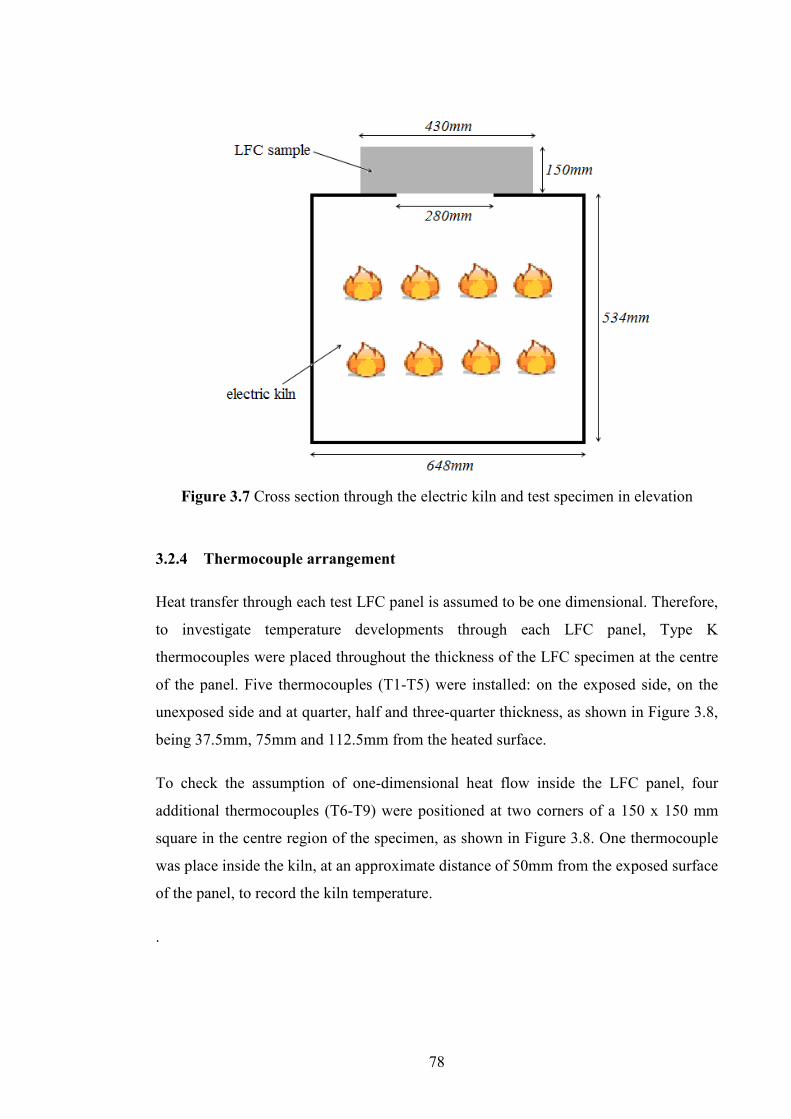
78
Figure 3.7 Cross section through the electric kiln and test specimen in elevation
3.2.4 Thermocouple arrangement
Heat transfer through each test LFC panel is assumed to be one dimensional. Therefore,
to investigate temperature developments through each LFC panel, Type K
thermocouples were placed throughout the thickness of the LFC specimen at the centre
of the panel. Five thermocouples (T1-T5) were installed: on the exposed side, on the
unexposed side and at quarter, half and three-quarter thickness, as shown in Figure 3.8,
being 37.5mm, 75mm and 112.5mm from the heated surface.
To check the assumption of one-dimensional heat flow inside the LFC panel, four
additional thermocouples (T6-T9) were positioned at two corners of a 150 x 150 mm
square in the centre region of the specimen, as shown in Figure 3.8. One thermocouple
was place inside the kiln, at an approximate distance of 50mm from the exposed surface
of the panel, to record the kiln temperature.
.

79
Figure 3.8 Thermocouple layout on LFC specimens on plan and throughout thickness
3.2.5 Kiln Temperature
LFC is considered to be non-reactive so its thermal properties are temperature
dependent only. Therefore, at this stage of the study an electric kiln was deemed
satisfactory as the source of heat and a Harrier Top Loading Electric Kiln was used for
the experiments. The kiln temperature was controlled in such a way that its
temperature-time relationship resembled that of the standard fire curve according to the
British Standard for fire resistance testing (BS476, 1987). Figure 3.9 shows the heating
curve achieved in the kiln, which is compared to a standard cellulosic fire curve
(BS476).
There is some difference between the heating curve and the standard temperature – time
curve. However, since this study relates the thermal properties of LFC to its
temperature, rather than that of the air, and the recorded LFC slab surface temperatures

80
were used as input data, the kiln simply acted as a heating source. It was not important
that its heating curve did not follow that of the standard fire curve exactly.
0
200
400
600
800
1000
1200
0 30 60 90 120 150 180 210
Time (min)
Tem
pera
ture (
°C)
Kiln Temperature
Standard Cellulosic Fire
Figure 3.9 Time-temperature curve for the kiln against standard cellulosic fire curve
3.2.6 Recorded temperature results inside LFC
To confirm 1-Dimensional heat transfer in the LFC slabs, thermocouples were installed
on the exposed and unexposed surfaces of the sample in the middle and near the four
corners. Figures 3.10 and 3.11 compare these observations. The three thermocouples on
each surface of the sample recorded very similar temperatures, thus confirming the one-
dimensional heat transfer assumption.

81
0
200
400
600
800
1000
0 15 30 45 60
Time (min)
Tem
pera
ture (
°C)
Observer Thermocouple (T7)
Observer Thermocouple (T9)
Mid point thermocouple (T5)
Figure 3.10 Temperature readings on top surface (exposed side) of one 650 kg/m3
density test observer thermocouples in (Test 2)
0
200
400
600
800
1000
0 10 20 30 40 50 60
Time (min)
Tem
pera
ture (
°C)
Observer Thermocouple (T6)
Observer Thermocouple (T8)
Mid point thermocouple (T5)
Figure 3.11 Temperature readings on bottom surface (unexposed side) of one 650
kg/m3 density test observer thermocouples in (Test 2)

82
The LFC specimen temperatures were monitored through 5 thermocouples which were
mounted at different thickness as been discussed in Section 3.2.3. For each density, 2
specimens were tested. Figure 3.12(a-d) and Figure 3.13(a-d) show the recorded
temperatures for 650 kg/m3 and 1000 kg/m3 at different thickness respectively. Close
agreement of test results were found for the two identical tests at different thickness for
both densities.
0
100
200
300
400
500
600
0 15 30 45 60 75 90 105 120 135
Time (min)
Tem
per
atu
re (
°C)
Temperature Test 1
Temperature Test 2
Figure 3.12(a) Recorded temperatures at different thickness for 650 kg/m3 density at
37.5mm from exposed side

83
0
100
200
300
400
500
600
0 15 30 45 60 75 90 105 120 135
Time (min)
Tem
per
atu
re (
°C)
Temperature Test 1
Temperature Test 2
Figure 3.12(b) Recorded temperatures at different thickness for 650 kg/m3 density at
70.0mm from exposed side
0
100
200
300
400
500
600
0 15 30 45 60 75 90 105 120 135
Time (min)
Tem
per
atu
re (
°C)
Temperature Test 1
Temperature Test 2
Figure 3.12(c) Recorded temperatures at different thickness for 650 kg/m3 density at
112.5mm from exposed side
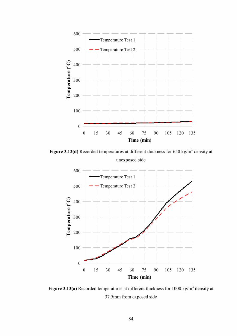
84
0
100
200
300
400
500
600
0 15 30 45 60 75 90 105 120 135
Time (min)
Tem
per
atu
re (
°C)
Temperature Test 1
Temperature Test 2
Figure 3.12(d) Recorded temperatures at different thickness for 650 kg/m3 density at
unexposed side
0
100
200
300
400
500
600
0 15 30 45 60 75 90 105 120 135
Time (min)
Tem
per
atu
re (
°C)
Temperature Test 1
Temperature Test 2
Figure 3.13(a) Recorded temperatures at different thickness for 1000 kg/m3 density at
37.5mm from exposed side

85
0
100
200
300
400
500
600
0 15 30 45 60 75 90 105 120 135
Time (min)
Tem
per
atu
re (
°C)
Temperature Test 1
Temperature Test 2
Figure 3.13(b) Recorded temperatures at different thickness for 1000 kg/m3 density at
75.0mm from exposed side
0
100
200
300
400
500
600
0 15 30 45 60 75 90 105 120 135
Time (min)
Tem
per
atu
re (
°C)
Temperature Test 1
Temperature Test 2
Figure 3.13(c) Recorded temperatures at different thickness for 1000 kg/m3 density at
112.5mm from exposed side

86
0
100
200
300
400
500
600
0 15 30 45 60 75 90 105 120 135
Time (min)
Tem
per
atu
re (
°C)
Temperature Test 1
Temperature Test 2
Figure 3.13(d) Recorded temperatures at different thickness for 1000 kg/m3 density at
unexposed side
Figure 3.14 show the comparison of the average temperature of the two LFC densities
at all four different locations of measurements. It can be seen from Figure 3.14 that the
recorded temperature growth at each location was less for LFC specimen of 1000 kg/m3
density compared to LFC specimen of 650 kg/m3 density. This is attributed to higher
thermal capacitance value (density times specific heat) for LFC specimen of 1000
kg/m3 density, which allow more heat to be absorbed thus slowing down the rate of
temperature rise.

87
0
100
200
300
400
500
600
0 15 30 45 60 75 90 105 120 135Time (min)
Tem
peratu
re (
°C)
37.5 mm (650 kg/m3)37.5 mm (1000 kg/m3)75.0 mm (650 kg/m3)75.0 mm (1000 kg/m3)112.5 mm (650 kg/m3)112.5 mm (1000 kg/m3)Unexposed (650 kg/m3)Unexposed (1000 kg/m3)
Figure 3.14 Comparison of the average temperature of the two LFC densities at all four
locations of measurements
3.3 DE�SITY A�D SPECIFIC HEAT TESTS
3.3.1 Effects of moisture content and dehydration reactions on LFC density
Hydrated cement paste is composed from four major compounds of tricalcium silicate
(3CaO•SiO2), dicalcium silicate (2CaO•SiO2), tricalcium aluminate (3CaO•A1203) and
tetracalcium aluminoferrite (4CaO•A1203•Fe203). The most significant products
involved in hydration reactions are calcium silicate hydrate (C-S-H) and portlandite,
also called calcium hydroxide (Ca(OH)2).
LFC contains free water and chemically bond water. The free water content in LFC
depends on the density (i.e., the free water content for the 650 kg/m3 density is 1.7% by
weight and for the 1000 kg/m3 density is 3.2% by weight based on experiment data).
Evaporation of the free and some of the chemically bond water will cause dehydration
in LFC, which will affect all the three items of thermal properties of LFC (density,
specific heat and thermal conductivity).

88
The dehydration process starts as early as 90°C. In the range of 90°C to 170°C, the
evaporable free water and part of the chemically bond water escapes. The evaporable
free water may be considered to have been completely eliminated by 170°C. Some
chemically bond water is also lost through decomposition of the Calcium Silicate
Hydrates (C-S-H) gel that takes place between 120°C and 140°C and decomposition of
ettringite around 120°C (Taylor, 1992). In the temperature range between 200°C and
300°C, some of the chemically bond water is released from further decomposition of
the C-S-H gel and the sulfoaluminate phases (3CaO.Al2O3.CaSO4.12H2O and
3CaO.Al2O3.3CaSO4.31H) of the cement paste (Taylor, 1992). Further dehydration
occurs at around 450°C, which corresponds to decomposition of Ca(OH) 2 → CaO +
H2O (Taylor, 1992) and it is completed at 530°C. At the second dehydration reaction,
75% of the chemically combined water is vaporised and the remaining 25% is then
evaporated at the third dehydration reaction.
70
75
80
85
90
95
100
105
0 100 200 300 400 500 600 700 800 900 1000Temperature (°C)
Ori
gin
al
Ma
ss (
%)
650 kg/m3
1000 kg/m3
1850 kg/m3 (Mortar)
Figure 3.15 Percentage of original density at different temperatures
The previously described three stages of dehydration are accompanied by water loss or
reduction in density of LFC. Figure 3.15 shows recorded densities of LFC at different
temperatures, as ratio of the original density for two different initial density values, 650
kg/m3 and 1000 kg/m3. These values are also compared to the density change of mortar
(density 1850 kg/m3).

89
The results presented in Figure 3.15 were obtained by directly weighing samples after
heating them to different temperatures. Usually thermo gravimetric analysis (TGA)
may be performed to determine changes in weight at increasing temperatures. However,
due to limitation in experimental facility, this study used manual recording according to
the following procedure: three 100×100mm x 100mm LFC cubes of each density (650,
1000 and 1850 kg/m3) were heated to different temperatures and then kept at the
desired temperature for 24 hours. Their weight was recorded afterwards to obtain
weight loss. The procedure was kept on until a maximum temperature of 1000°C.
The three curves are similar and the three dehydration phases can be clearly seen in
Figure 3.15. This figure also shows a further weight loss phase, occurring between
750°C and 850°C, which can be assigned to the release of carbon dioxide (CO2) from
calcium carbonate (CaCO3) (Taylor, 1992):
CaCO3 → CaO + CO2
Table 3.2 summarises the density change values for the four phases (three phases of
dehydration and final phase of CO2 release) of weight loss.
Table 3.2 Density change values due to the dehydration process
Remaining density at the end of each dehydration process (kg/m3) Initial
density
(kg/m3)
(1th)
completed at
170°C
(2nd)
completed at
300°C
(3rd)
completed at
530°C
(Final)
completed at
850°C
650 637 603 590 579
1000 973 903 881 860
1850 1763 1613 1569 1500
3.3.2 Specific heat for heat transfer analysis only
LFC can be considered as a non-reactive material and therefore its thermal properties
can be considered to be temperature dependent only. Given that there is mass transfer
involving water movement, precise treatment of thermal performance of LFC in fire
should include combined heat and mass transfer. However, mass transfer can be rather
complex to deal with and many of the mass transfer related material properties are

90
different to obtain. An alternative treatment is to carry out heat transfer analysis only,
but taking into consideration the effects of mass transfer in heat transfer properties. The
validity of such a treatment has been demonstrated by Ang and Wang (2004) on
gypsum plaster, which has similar mass and heat transfer phenomena. The main effect
of mass transfer, caused by moisture movement, is included in heat transfer analysis by
modifying the specific heat of LFC. This will be explained in detail in Section 4.5.1.
The specific heat of LFC may be divided into two parts: the base value corresponding
to a mixture of the dry components and the effect of water evaporation. The base value
of the dry components may be calculated using Rule of mixtures as follows (Wang HB,
1995):
pii
n
ip CFC 1−∑= … (3.1)
where Cp is the overall specific heat capacity, Cpi is component specific heat, Fi is the
volume fraction of each component and ∑ Fi = 1.
According to the mixture law and bearing in mind the three phase of dehydration, the
base value of specific heat of LFC should consist of four segments: from ambient
temperature to the start of the first phase, from the end of the first phase to the start of
the second phase, from the end of the second phase to the start of the third phase, and
after the end of the third phase. However, existing literature, including fire resistant
design codes for concrete structures such as EN 1992-1-2 (2004) and EN 1994-1-2
(2005), suggest that the base value which may be taken as a constant value is that at
ambient temperature. Since LFC differs from normal concrete only in terms of density,
the base value of LFC is also considered constant over the entire temperature range.
Tables 3.3 and 3.4 give the weights of different components of the two densities of LFC
(650 and 1000 kg/m3) and the base value of specific heat at ambient temperature.

91
Table 3.3 Base value of specific heat for 650 kg/m3 density
Material
Weight
per 100
litre of
LFC
(kg)
Fractional
weight
(%)
Density
(kg/m3)
Fractional
volume
(%)
Specific
heat of
component
(J/kg°C)
Contribution
to specific
heat of LFC
(J/kg°C)
Cement 36.77 62.01 3130 47.59 920 571
Sand 18.38 31.01 2090 35.64 800 248
Water
with
foam
4.14 6.98 1000 16.77 4180 292
Total 57.97 100.00 - 100.00 - 1110
Table 3.4 Base value of specific heat for 1000 kg/m3 density
Material
Weight
per 100
litre of
LFC
(kg)
Fractional
weight
(%)
Density
(kg/m3)
Fractional
volume
(%)
Specific
heat of
component
(J/kg°C)
Contribution
to specific
heat of LFC
(J/kg°C)
Cement 53.96 58.89 3130 42.21 920 542
Sand 26.98 29.44 2090 31.60 800 236
Water
with
foam
10.69 11.67 1000 26.18 4180 488
Total 94.32 100.00 - 100.00 - 1265
In addition to the base value of specific heat, heat is also required to evaporate water
from LFC. Therefore, the specific heat of LFC should be obtained from (Ang and
Wang, 2004):
adddrypp CCC += , … (3.2)
where Cp,dry is 1110 J/kg°C for LFC of 650 kg/m3 and 1265 J/kg°C for LFC of 1000
kg/m3 as calculated previously (Tables 3.3 and 3.4) and Cadd is the additional heat

92
required to drive off water. Cadd should be variable during the water evaporation
temperature range to reflect that start and completion of water evaporation are gradual
processes. A triangular distribution of specific heat over the water evaporation
temperature range is typically assumed as shown in Figure 3.16. In this figure, c∆ is the
average additional specific heat.
0 10 20 30 40 50 60
FT (°C)
Ad
dit
ion
al
spec
ific
hea
t
2∆c
Figure 3.16 Additional specific heat for evaporation of free water (Ang and
Wang, 2004).
Many previous studies (Noumowe, 1995), (Taylor, 1992) have assumed that water is
simply evaporated at the evaporation temperature range. Consequently, the area within
the triangle in Figure 3.16 is the latent heat of evaporation of water. However, Wang
HB (1995) suggested that due to water movement, this was not sufficient and a higher
value of specific heat should be applied. This has been confirmed by Ang and Wang
(2004) who carried out a combined heat and mass analysis. In this study, the average
additional specific heat for LFC was calculated as follows:
)/(1026.2 6
CkgJfeT
c °××∆×
=∆ … (3.3)

93
in which the value of 2.26 x 10⁶ J/kg is the latent heat of evaporation of water, ∆c is the
average additional specific heat, e is dehydration water content (percentage by total
weight), ∆T is the magnitude of the temperature interval during which water is
evaporated and f is a modification factor accounting for water movement. A value of f
=1.4 was used. This value was established by Ang and Wang (2004) for gypsum. Ang
and Wang who also found that this value to be relatively insensitive to different values
of permeability provided the permeability is high. It was considered that both LFC and
gypsum plaster are highly permeable materials so they should have a similar value of f.
Since temperature rise in LFC is much more sensitive to changes in thermal
conductivity than in specific heat, it was decided not worthwhile to refine the value of f.
According to this procedure, the peak values of additional specific heat for LFC of 650
kg/m3 and 1000 kg/m3 densities are 2455 J/kg°C and 3796 J/kg°C respectively.
Since there are three phases of dehydration as explained previously, the above
additional specific heat should be applied during each dehydration phase. Referring to
the existing literature for the base value of specific heat, including fire resistance design
codes for concrete, only the first phase of dehydration due to evaporation of the free
water should be considered. Therefore, the specific heat – temperature relationship of
concrete has only one peak, corresponding to the first phase. This appears to have been
confirmed from the experimental results of this research. As can be seen from Figure
3.14, the temperature plateau between 90-170oC is clearly noticeable, reflecting the first
phase of dehydration. Afterwards, the temperature development is smooth and
continuous without any plateau at the other two dehydration phases. Therefore, in this
research, the additional specific heat will only be applied to the first phase of
dehydration. As a summary, Figure 3.17 shows the temperature-dependent specific heat
of LFC for both densities of 650 kg/m3 and 1000 kg/m3.

94
0
500
1000
1500
2000
2500
3000
3500
4000
0 100 200 300 400 500 600 700 800 900 1000
Temperature (°C)
Sp
ecif
ic h
eat
(J/k
g.°
C)
650 kg/m3
1000 kg/m3
Figure 3.17 Specific heat of LFC (650 and 1000 kg/m3 density) versus temperature
3.4 THERMAL CO�DUCTIVITY RELATED TESTS
As mentioned in the introduction section, two methods will be used to obtain thermal
conductivity of LFC. One is direct measurement method, using the Hot Guarded Plate
test. The other one combines analytical modelling and transient heating test. For the
latter, the analytical model treats LFC as a porous material and it is necessary to
measure the porosity and pore size. These results are presented in this section.
3.4.1 Hot Guarded Plate Test
The HGP test followed the ASTM procedure in reference (ASTM, 1997). This
particular test was conducted in concrete lab, University of Salford due to unavailability
of such equipment in University of Manchester. The hot guarded plate test is generally
recognized as the primary absolute method for measurement of the thermal
transmission properties of homogeneous insulation materials in the form of flat slabs.
This steady-state test method has been standardized by ASTM International as ASTM
Standard Test Method C 177.
The basic HGP method consists principally of a hot plate and a cold plate. In a HGP
test, the test specimen is placed on a flat plate heater assembly consisting of an
electrically heated inner plate (main heater) surrounded by a guard heater. The guard

95
heater is carefully controlled to maintain the same temperature on both sides of the gap
separating the main and the guard heaters. This prevents lateral heat flow from the main
heater and ensures that heat from the electric heater flows in the direction of the
specimen. On the opposite side of the specimen are additional flat plate heaters (cold
plate) that are controlled at a fixed temperature selected by the operator. For a given
heat input to the main heater, the hot plate assembly rises in temperature until the
system reaches equilibrium.
The final hot plate temperature depends on the electrical power input, the thermal
resistance of the specimen and the temperature of the cold plate. The average thermal
conductivity, k, of the specimen is determined from the Fourier heat flow equation as
follow:
∆
×=T
d
A
Wk 1 … (3.4)
where W is the electrical power input to the main heater, A is the main heater surface
area, KT is the temperature difference across the specimen, and d is the specimen
thickness.
Table 3.5 presents the HGP test results.
Table 3.5 Thermal conductivity of LFC at different temperatures obtained
through Hot Guarded Plate tests
Thermal conductivity at different temperatures (W/mK) Dry
density
(kg/m3) 20°C 90°C 105°C 150°C 170°C 180°C 200°C 250°C
650 0.23 0.23 0.21 0.16 0.13 0.13 0.14 0.15
1000 0.31 0.31 0.29 0.25 0.24 0.24 0.24 0.25
1850 0.48 0.48 0.47 0.45 0.43 0.43 0.43 0.44
3.4.2 Porosity and thermal conductivity of air
The porosity value of LFC was determined through the Vacuum Saturation Apparatus
(Cabrera and Lynsdale, 1988). The measurements of LFC porosity were conducted on
slices of 68mm diameter cores cut out from the centre of 100mm cubes. Two densities,

96
650kg/m3 and 1000 kg/m3, were considered. The specimens were dried at 105°C until
constant weight had been attained and were then placed in a desiccator under vacuum
for at least 3 hours, after which the desiccator was filled with de-aired, distilled water.
The porosity was calculated using the following equation:
100)(
)(×
−
−=
watsat
drysat
WW
WWε … (3.5)
where ε is the porosity (%), Wsat is the weight in air of saturated sample, Wwat is the
weight in water of saturated sample and Wdry is the weight of oven-dried sample. The
measured results are given in Table 3.6.
Table 3.6 Porosity of LFC obtained through Vacuum Saturation for
thermal properties test
Sample
Dry density
(kg/m3)
Wdry
Saturated in air
(kg/m3)
Wsat
Saturated in water
(kg/m3)
Wwat
Porosity
(%)
650/1 650 899 565 74.6
650/2 649 912 562 75.1
650/3 653 908 571 75.7
1000/1 1004 1294 719 50.4
1000/2 1007 1287 737 50.9
1000/3 1002 1278 725 49.9
For analysis purpose, the porosity values are taken as 75% and 50% for LFC of
densities of 650 and 1000 kg/m3 respectively.
To obtain the thermal conductivity of gas in the air pores, it is necessary to include the
effects of radiation within the pores at high temperatures. Assuming the air pores may
be represented by uniform distribution of spherical pores of diameter de, the effective
thermal conductivity of the gas ( gλ ) at elevated temperatures may be analytically
derived to give the following equation (Yuan, 2009):
3717.04 43
210815.4 TdT eg σλ ×+×= − … (3.6)

97
where the first term is the gas thermal conductivity without the effect of thermal
radiation and the second term represents the effect of radiation within the air pores.
Although there is also convection with the air pores, due to the small size of the pores
(never larger than 5mm), natural convection in the pores can be neglected (Burns and
Tien, 1979).
3.4.3 Pore size measurements
In order to calculate the effective thermal conductivity of gas inside the air pores, it is
necessary to establish the pore size. For the purpose of this study, the specimen
preparation for the measurement of the pore size was slightly different then from
recommended by ASTM C 457. ASTM C 457 specified the size and thickness of the
specimen and length of travel in the linear traverse method (LTM), based on the size of
aggregate. Mixtures from this study, however, do not contain any coarse aggregate but
consist of high amounts of air (foam). To ensure the stability of the air pore walls
during polishing, particularly in weaker specimens (lower density), all the specimens
were vacuum-impregnated with slow-setting epoxy. To ensure consistency in results,
all the specimens were prepared using similar techniques under the same environmental
conditions, as follows.
Foremost, the specimens of 45 x 45 mm size with a minimum thickness of 15 mm were
cut from the centre of two randomly selected 100 mm cubes using a diamond cutter.
The face of the specimen was cut perpendicular to the casting direction. Sized
specimens were saturated in acetone to stop further hydration reaction before drying at
105 °C. To ensure the stability of the air-pore walls during polishing, the dried and
cooled specimens were vacuum impregnated with slow-setting epoxy. The impregnated
specimens were polished as per ASTM C 457. After polishing and cleaning, the
specimens were dried at room temperature for 1 day. Finally, an effective size 40 x 40
mm was considered for pore size measurement.
The pore size were measured according to ASTM C 457 under a microscope with a
magnification of 60x on two specimens, prepared as per the procedure described
previously, for each LFC specimen. Image analysis system consisted of an optical
microscope and a computer with image analysis software. Figure 3.18 shows
microscopic images of the internal pore structure of the 1000 and 650 kg/m3 density
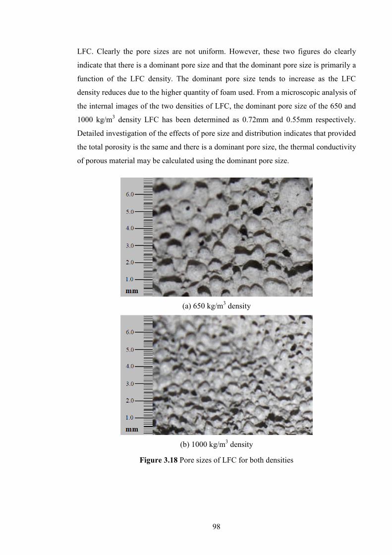
98
LFC. Clearly the pore sizes are not uniform. However, these two figures do clearly
indicate that there is a dominant pore size and that the dominant pore size is primarily a
function of the LFC density. The dominant pore size tends to increase as the LFC
density reduces due to the higher quantity of foam used. From a microscopic analysis of
the internal images of the two densities of LFC, the dominant pore size of the 650 and
1000 kg/m3 density LFC has been determined as 0.72mm and 0.55mm respectively.
Detailed investigation of the effects of pore size and distribution indicates that provided
the total porosity is the same and there is a dominant pore size, the thermal conductivity
of porous material may be calculated using the dominant pore size.
(a) 650 kg/m3 density
(b) 1000 kg/m3 density
Figure 3.18 Pore sizes of LFC for both densities

99
3.5 ADDITIO�AL SPECIME�S FOR I�DICATIVE STUDY O� FIRE
RESISTA�CE PERFORMA�CE OF LFC PA�EL
As mentioned in Chapter 1, one of the objectives of this research is to investigate
feasibility of using LFC in lightweight residential construction, based on insulation
performance for fire resistance. To execute this study, additional LFC specimens of
800, 1200 and 1400 kg/m3 density were cast to determine the base input values such as
density changes, moisture content, specific heat, porosity and pore size which are
essential parameters to validate the one dimensional heat transfer analysis program. The
thermal conductivity of LFC for all densities was obtained through Hot Guarded Plate
test and the values are given in Table 3.7. The specific heat was in the same way as that
for the 650 kg/m3 and 1000 kg/m3 density, described in Section 3.3.2, but with
appropriate free moisture content. The porosities were also established through Vacuum
Saturation and pore sizes were determined for each density through image analysis of
the internal structure as discussed in Section 3.4.2.
Table 3.8 demonstrates the density change values for the four phases (three phases of
dehydration and final phase of CO2 release) of weight loss, Table 3.9 summarises the
free water content, base specific heat and additional specific heat values for all LFC
densities and finally Table 3.10 demonstrates the porosity for all LFC densities and
variation of effective pore sizes.
Table 3.7 Thermal conductivity of LFC for different density
Hot guarded plate test thermal
conductivity (W/mK)
Calculated ambient temperature
thermal Conductivity (W/mK) Density
(kg/m3) Base value Dry Base value Dry
800 0.272 0.193 0.269 0.182
1200 0.379 0.307 0.361 0.272
1400 0.429 0.362 0.402 0.323

100
Table 3.8 Density change values due to the dehydration process
Initial
density
(kg/m3)
Remain
density after
first
dehydration
(kg/m3)
Remain density
after second
dehydration
(kg/m3)
Remain
density after
third
dehydration
(kg/m3)
Remain density
after final
dehydration
(kg/m3)
800 783 730 712 702
1200 1165 1069 1043 1010
1400 1351 1238 1208 1170
Table 3.9 Calculated free water content, chemically bound water, specific heat and
additional specific heat values
Dry density
(kg/m3)
Free water
(% by weight)
Specific heat
(J/kg°C)
Additional specific heat at
first dehydration process
(J/kg°C)
800 2.4 1193 3091
1200 4.5 1313 4873
1400 5.3 1346 5538
Table 3.10 Porosity and effective pore size values
Dry density
(kg/m3)
Porosity
(%)
Effective pore size
(mm)
800 61 0.62
1200 37 0.49
1400 26 0.37
3.6 SUMMARY
This chapter has presented the experimental results necessary for determining thermal
properties of LFC. In particular, in Chapter 4, an analytical model for thermal
conductivity, based on treating LFC as porous material, will be acknowledged. In
regards to use of this model, it is necessary to have information of porosity and pore

101
size. This chapter has laid out the experimental data. The thermal conductivity –
temperature relationship of LFC will be obtained by calibrating the analytical model
against 1-Dimensional transient heat conduction tests. The results of these heat
conduction tests have also been discussed. For validation of the analytical model,
Guarded Hot Plate tests were conducted to directly give thermal conductivity of LFC
up to temperature 250°C.
102
CCHHAAPPTTEERR 44
VVAALLII DDAATTIIOO�� OOFF MMOODDEELLSS OOFF TTHHEERRMMAALL PPRROOPPEERRTTIIEESS
OOFF LLFFCC
4.1 I�TRODUCTIO�
One important objective of this research is to establish an analytical approach to obtain
thermal properties, particularly thermal conductivity, of LFC. Chapter 3 has described
the experiments and this chapter will explain how the analytical approach is developed
and validated.
4.2 �UMERICAL A�ALYSIS
Rahmanian (2008) has developed and implemented a computer program to model the
transient heat transfer through LFC in the familiar environment of Microsoft Excel
using VBA based on one-dimensional Finite Difference formulations. The modelling
procedure has been systematically validated by comparisons with a number of
analytical solutions and simulation results using ABAQUS/Standard. The next section
will describe the basis of the modelling method which includes the development of one-
dimensional Finite Difference formulation which can be used to solve transient heat
conduction problems for porous material.
4.2.1 One-Dimensional Finite Difference Formulation
Assuming a homogenous and isotropic material, the general three-dimensional transient
heat-conduction equation (based on Fourier’s law of conduction) in Cartesian
coordinates is (Holman, 2002):
∂∂
∂∂
+
∂∂
∂∂
+
∂∂
∂∂
=∂∂
z
Tk
zy
Tk
yx
Tk
xt
Tcρ ……… (4.1)

103
where
T(x,y,z,t) is temperature (˚C);
k(T) is temperature dependent thermal conductivity (W/mK);
ρ is material density (kg/m3);
c is specific heat of material (J/kg°C);
t is time (sec);
x, y, z are Cartesian coordinates.
The right hand side of Equation 4.1 stand for the net heat conduction in a solid material,
whereas the left hand side represents the accumulated internal energy.
If the thickness of the LFC panel is small in comparison to the other dimensions, the
problem will reduce to a one dimensional heat transfer analysis, i.e. the heat flow is
perpendicular to the face except near the edges. Hence, the governing Equation 4.1 with
no heat generation reduces to:
∂
∂∂∂
=∂
∂x
txTTk
xt
txTc
),()(
),(ρ …………………. (4.2)
where 0 ≤ x ≤ L, for t > 0, L is the thickness of the panel
Assuming a homogeneous material and choosing the explicit method, the temperature
of a volume cell (Figures 4.1 and 4.2) at a time step is computed directly based on the
temperatures of the adjacent cells in the last time step which leads to a very
straightforward scheme of computation (Wang HB, 1995):
(i) For a typical node m within the material (Figure 4.1):
)]21
()(2
[0,1,1
1,11,10 −+
+
+=′
+−
++−−
FT
kk
TkTkFT m
mmmm
mmmmmm
m …. (4.3)

104
where F0 is defined as:
2
,1,10 )(2
)(
xc
tkkF
mmmm
∆
∆+= +−
ρ …………… ……………. (4.4)
mT ′ is the temperature of m in the subsequent time step and jik , is the thermal
conductivity at the average temperature of cells i and j:
)2
(,ji
ji
TTkk
+= ……………………………….... (4.5)
Numerical stability under the explicit scheme requires:
)(
)(
,1,1
2
mmmm kk
xct
+− +∆
≤∆ρ
……………………………... (4.6)
(ii) For a boundary node, when subjected to convective and radiative boundary
conditions (Figure 4.2):
xc
tTTeT
k
xh
FT
k
xhTFT
∆∆
+−++∆
−−+∆
+= ∞∞ ρσφ
2])273()273[())1
2
1([2 4
14
1101
20'
1 .(4.7)
where F0 is 21
0 )( xc
tkF
∆
∆=ρ
)(Th is convection heat transfer coefficient (W/m2K);
∞T is the ambient temperature (°C);
φ is a geometric “view factor”
e is the effective emissivity
σ is Stefan-Boltzmann constant (5.67 x 10⁻⁸ W/m2.K4).
Numerical stability limits the time step to:
1
1
41
111
2
])273(
1[)(5.0 −+
⋅∆
+∆
+∆
≤∆T
T
k
xE
k
xh
k
xct
σφρ … (4.8)

105
Heat flow direction
m-1 m m+1
1
∆x
Figure 4.1 Finite Difference discretization for node m within the material
Heat flow direction
2 1
1
∆x
Figure 4.2 Finite Difference discretization for boundary node
4.2.2 Initial and Boundary Conditions
LFC panel is assumed to have a uniform initial temperature equal to the ambient
temperature. On the unexposed boundary, the convective heat transfer coefficient (h) is
assumed to be constant and the value is taken as 10 W/m2K. The emissivity of the
surface depends on the material. For concrete, the surface emissivity will be taken as
0.92 (Ozisik, 1985). The exposed boundary conditions are the recorded temperatures on
the exposed surface of fire test specimens.
4.2.3 Validation of the heat conduction model
Sections 4.2.1 and 4.2.2 have comprehensively extracted the Finite Difference
formulations to model the one-dimensional transient heat transfer through LFC and its
initial and boundary conditions. It is important to verify the accuracy of this model
through comparison with the available analytical and numerical solutions. To
accomplish this validation, 3 different approaches have been taken as follows:

106
1. Verification of the conductive heat transfer simulation through a panel (referred
to as case 1)
2. Verification of the convective heat transfer at boundaries of a panel (referred as
to case 2)
3. Verification of the conductive heat transfer simulation with temperature-to
dependent material properties (referred as case 3).
For case 1 and 2, analytical solutions are presented with constant material properties of
LFC. Nevertheless no analytical solution is established when thermal properties of
material change with temperature (case 3). Therefore, numerical simulation results
using the generic commercial finite element package, ABAQUS, are employed to
corroborate the Finite Difference formulations.
4.2.3.1 Conduction Heat Transfer with Constant Material Properties
Consider a one-dimensional heat transfer through LFC panel with thickness l and
constant thermal conductivity k . The initial temperature of the panel is uniform and
indicated by 0T (Figure 4.3). If both surfaces of the LFC panel are suddenly changed to
zero temperature (0°C), temperature development through the thickness of the panel at
time t can be calculated as follow (Carslaw and Jaeger, 1959):
4 2 2 21 (2 1)(2 1) /0 sin(2 1)0
T n xn t lT e
n ln
πα ππ
∞ +− += ∑+=
…. (4.9)
where k
cα
ρ= , ρ is the density of the material and c is the specific heat.
Figure 4.3 LFC panel with thickness l, both boundaries kept at zero temperature
Analysis has been carried out for an example of case 1 (Figure 4.3) with the material
properties indicated in Table 4.1.
l
Tb=0°C (t >0)
T=T0 ; ( 0=t )
x

107
Table 4.1 Material properties of LFC to analyse example of case 1
LFC properties Values
Density (ρ) 650 kg/m3
Thickness of panel (l) 30 mm
Thermal conductivity (k) 0.206 W/mK
Specific heat (c) 1110 J/kg.°C
Initial temperature (T0) 20°C
The temperature development of this example is achieved through both the analytical
method (Equation 4.9) and the Finite Difference method. The results are compared in
Figures 4.4 and 4.5. The thickness of the panel is divided into 6 elements and
temperatures are calculated for the nodes indicating each element (5 internal nodes and
2 boundary nodes) and the time step of 5 seconds is used for this Finite Difference
method. The infinite series in Equation 4.9 has been restricted to only 12 members for
calculation purposes. It can be seen in Figures 4.4 and 4.5 that Finite Difference method
can offer very accurate results for heat transfer analysis in solids with constant thermal
properties regardless of its simple approach.
1 min
4 min
8 min
0
5
10
15
20
25
0 5 10 15 20 25 30
thickness (mm)
Tem
per
atu
re (
°C)
Analytical Solution
FD Solution
Figure 4.4 Temperature distribution across the thickness of a 30mm example panel
attained by analytical method and Finite Difference method
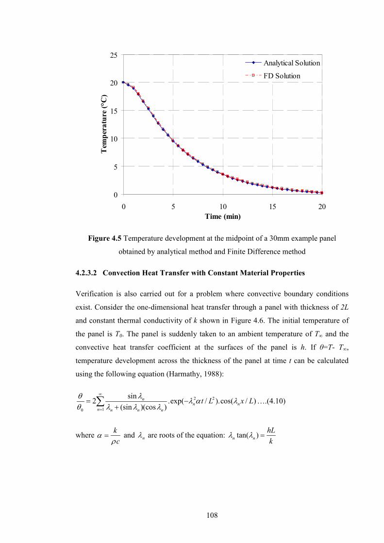
108
0
5
10
15
20
25
0 5 10 15 20Time (min)
Tem
per
atu
re (
°C)
Analytical Solution
FD Solution
Figure 4.5 Temperature development at the midpoint of a 30mm example panel
obtained by analytical method and Finite Difference method
4.2.3.2 Convection Heat Transfer with Constant Material Properties
Verification is also carried out for a problem where convective boundary conditions
exist. Consider the one-dimensional heat transfer through a panel with thickness of 2L
and constant thermal conductivity of k shown in Figure 4.6. The initial temperature of
the panel is T0. The panel is suddenly taken to an ambient temperature of T∞ and the
convective heat transfer coefficient at the surfaces of the panel is h. If θ=T- T∞,
temperature development across the thickness of the panel at time t can be calculated
using the following equation (Harmathy, 1988):
2 2
10
sin2 .exp( / ).cos( / )
(sin )(cos )n
n n
n n n n
t L x Lλθ
λ α λθ λ λ λ
∞
=
= −+∑ ….(4.10)
where k
cα
ρ= and nλ are roots of the equation: tan( )n n
hL
kλ λ =
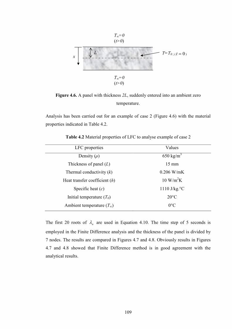
109
Figure 4.6. A panel with thickness 2L, suddenly entered into an ambient zero
temperature.
Analysis has been carried out for an example of case 2 (Figure 4.6) with the material
properties indicated in Table 4.2.
Table 4.2 Material properties of LFC to analyse example of case 2
LFC properties Values
Density (ρ) 650 kg/m3
Thickness of panel (L) 15 mm
Thermal conductivity (k) 0.206 W/mK
Heat transfer coefficient (h) 10 W/m2K
Specific heat (c) 1110 J/kg.°C
Initial temperature (T0) 20°C
Ambient temperature (T∞) 0°C
The first 20 roots of nλ are used in Equation 4.10. The time step of 5 seconds is
employed in the Finite Difference analysis and the thickness of the panel is divided by
7 nodes. The results are compared in Figures 4.7 and 4.8. Obviously results in Figures
4.7 and 4.8 showed that Finite Difference method is in good agreement with the
analytical results.
T=T0 ; ( 0=t ) x
T∞=0
(t>0)
T∞=0
(t>0)
L

110
25 min
12 min
2 min
0
5
10
15
20
25
0 5 10 15 20 25 30
thickness (mm)
Tem
per
atu
re (
°C)
Analytical Solution
Finite Difference Solution
Figure 4.7 Temperature distributions across the thickness of a 30mm example panel
with convective boundary condition attained by analytical method and Finite
Difference method
0
5
10
15
20
25
0 5 10 15 20Time (min)
Tem
per
atu
re (
°C)
Analytical Solution
Finite Difference Solution
Figure 4.8 Temperature developments at the surface of a 30mm example panel with
convective boundary condition attained by analytical method and Finite Difference
method

111
4.2.3.3 Heat Transfer with Temperature-Dependent Thermal Properties
The thermal properties LFC are temperature-dependant. Since analytical solutions for
heat transfer through this material is not available, another numerical method, Finite
Element analysis, is employed for validation of Finite Difference analysis. For
validation purpose, a 30mm LFC panel initially at 25°C is considered. The temperature-
dependent thermal properties of the LFC panel are modelled as explained in Section
3.3.2 and Section 4.3, with density of 650 kg/m3 at ambient temperature. One surface
of the panel is exposed to high temperatures and the other side faces the ambient
temperature of 25°C. Figure 4.9 illustrates the temperature curve obtained
experimentally on the exposed surface of the panel and compares the temperature
predictions of the unexposed side by the proposed Finite Difference analysis and by
Finite Element analysis using the common software package, ABAQUS. The validity
of Finite Difference formulations is confirmed yet again.
0
200
400
600
800
1000
1200
0 20 40 60 80 100Time (min)
Tem
per
atu
re (
°C)
Exposed Surface
ABAQUS Solution
Finite Difference Solution
Figure 4.9 Temperature developments on the unexposed surface of a 30mm LFC panel
attained by ABAQUS (Finite Element analysis) and Finite Difference method
The validation of Finite Difference formulations confirmed that even though explicit
Finite Difference method is a fairly simple algorithm, it can still offer very precise
results compared to analytical methods or other complicated numerical ones.
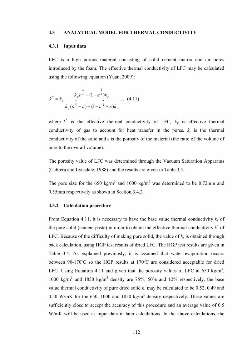
112
4.3 A�ALYTICAL MODEL FOR THERMAL CO�DUCTIVITY
4.3.1 Input data
LFC is a high porous material consisting of solid cement matrix and air pores
introduced by the foam. The effective thermal conductivity of LFC may be calculated
using the following equation (Yuan, 2009):
sg
sg
s
kk
kkkk
)1()(
)1(
3
2
3
2
3
2
3
2
*
εεεε
εε
+−+−
−+= … (4.11)
where k* is the effective thermal conductivity of LFC, kg is effective thermal
conductivity of gas to account for heat transfer in the pores, ks is the thermal
conductivity of the solid and ε is the porosity of the material (the ratio of the volume of
pore to the overall volume).
The porosity value of LFC was determined through the Vacuum Saturation Apparatus
(Cabrera and Lynsdale, 1988) and the results are given in Table 3.5.
The pore size for the 650 kg/m3 and 1000 kg/m3 was determined to be 0.72mm and
0.55mm respectively as shown in Section 3.4.2.
4.3.2 Calculation procedure
From Equation 4.11, it is necessary to have the base value thermal conductivity ks of
the pure solid (cement paste) in order to obtain the effective thermal conductivity k* of
LFC. Because of the difficulty of making pure solid, the value of ks is obtained through
back calculation, using HGP test results of dried LFC. The HGP test results are given in
Table 3.4. As explained previously, it is assumed that water evaporation occurs
between 90-170oC so the HGP results at 170oC are considered acceptable for dried
LFC. Using Equation 4.11 and given that the porosity values of LFC at 650 kg/m3,
1000 kg/m3 and 1850 kg/m3 density are 75%, 50% and 12% respectively, the base
value thermal conductivity of pure dried solid ks may be calculated to be 0.52, 0.49 and
0.50 W/mK for the 650, 1000 and 1850 kg/m3 density respectively. These values are
sufficiently close to accept the accuracy of this procedure and an average value of 0.5
W/mK will be used as input data in later calculations. In the above calculations, the

113
effect of radiation within pores was not considered because of the relatively low
temperature.
The thermal conductivity – temperature relationship of LFC may be divided into three
segments: (1) an initially flat part with the thermal conductivity constant as that at
ambient temperature, until water evaporation starts at the assumed temperature of 90oC;
(2) a linearly decreasing segment until all the water has evaporated and the LFC is dry,
which is assumed at 170oC; (3) increasing thermal conductivity with temperature due to
radiation in the pores. The third segment is described using Equation 4.11.
For the LFC thermal conductivity at ambient temperature, the directly measured result
may be used. However, this value can also be derived from the value of dried LFC,
measured at 170°C. In this calculation, the LFC may be considered to be part dry LFC
and part water and Equation 4.12, based on volume fraction, may be used to calculate
the thermal conductivity of LFC at ambient temperature.
drywwwamb kVkVk )1( −+= … (4.12)
where kamb is the LFC thermal conductivity at ambient temperature; Vw is the volume
percentage of water; kw is the thermal conductivity of water (0.58 W/mK) and kdry is the
thermal conductivity of dry LFC (value in Table 3.4 for 170oC).
For LFC density of 650 kg/m3, kdry = 0.131 W/mK (Table 3.4), Vw = 0.1677 (Table 3.2),
giving kamb = 0.206 W/mK. For LFC density of 1000 kg/m3, kdry = 0.235 W/mK (Table
3.4), Vw = 0.2618 (Table 3.3), giving kamb=0.325 W/mK. These calculated ambient
temperature thermal conductivity values are close to the HGP test values of 0.226 and
0.309 W/mK respectively.
Figure 4.10 shows the calculated effective thermal conductivity of LFC for the two
densities considered in this study and compare these calculated values with those
directly measured using the HGP method (Table 3.4 values). The agreement is
excellent, but the analytical model is able to give the thermal conductivity –
temperature relationships above 250°C.
To summarise, the following input data are required for determining thermal
conductivity – temperature relationship of LFC:

114
Thermal conductivity of cement paste at ambient temperature (0.5 W/mK); Volume
fracture of water at ambient temperature: Vw; Porosity; Pore size.
The calculation procedure is as follows:
1. Calculate thermal conductivity of dried LFC at ambient temperature: use
Equation 4.11;
2. Followed by calculating thermal conductivity of LFC at ambient temperature:
use Equation 4.12;
3. The thermal conductivity is taken as constant at the value calculated in step 2
from ambient temperature to 90°C;
4. The thermal conductivity reduces linearly from the value calculated in step 2 at
90°C to the value calculated in step 1 at 170°C;
5. Equation 4.11 is used for thermal conductivity at temperatures above 170°C.
0.00
0.10
0.20
0.30
0.40
0 200 400 600 800 1000
Temperature (°C)
Th
erm
al
Co
nd
ucti
vit
y (
W/m
°C)
650 kg/m3 (hot guarded plate conductivity model)
650 kg/m3 (proposed conductivity model)
1000 kg/m3 (hot guarded plate conductivity model)1000 kg/m3 (proposed conductivity model)
Figure 4.10 Effective thermal conductivity of LFC for 650 kg/m3 and 1000 kg/m3
densities

115
4.4 VALIDATIO� OF THERMAL PROPERTIES MODELS
In order to validate the proposed thermal property models for LFC presented in Chapter
3, thermal property values from these models were used as input material properties in
the one-dimensional heat transfer program to predict temperature developments inside
the LFC slab test samples described in Section 3.2.2 of this thesis. As mentioned in
Section 3.2.6, it is acceptable to assume that heat transfer in the test samples is one-
dimensional in the thickness direction of the LFC panel.
Measured experimental temperatures at all recording locations of the test specimens for
both densities of LFC were compared with numerical analysis results, to provide
comprehensive validation of the thermal property models proposed in Section 3.3 and
4.3. Thermal property values (theoretical thermal property model results) are
considered and their prediction results compared.
As mentioned previously, the exposed surface temperatures are used as input data in the
heat transfer analysis to eliminate uncertainty in the thermal boundary condition on the
exposed side. Figures 4.11-4.14 compare the measured and numerical analysis results
for the 650 kg/m3 density specimens and Figures 4.15-4.18 are for the 1000 kg/m3
density specimens.

116
0
100
200
300
400
500
600
0 15 30 45 60 75 90 105 120 135
Time (min)
Tem
per
atu
re (
°C)
Proposed thermal property model
Temperature Test 1
Temperature Test 2
Figure 4.11 Comparison between test results and numerical analysis at 37.5mm from
exposed surface for the 650 kg/m3 density specimens
0
100
200
300
400
500
600
0 15 30 45 60 75 90 105 120 135
Time (min)
Tem
per
atu
re (
°C)
Proposed thermal property model
Temperature Test 1
Temperature Test 2
Figure 4.12 Comparison between test results and numerical analysis at 75.0mm from
the exposed surface for the 650 kg/m3 density specimens

117
0
100
200
300
400
500
600
0 15 30 45 60 75 90 105 120 135
Time (min)
Tem
per
atu
re (
°C)
Proposed thermal property model
Temperature Test 1
Temperature Test 2
Figure 4.13 Comparison between test results and numerical analysis at 112.5mm from
the exposed surface (mid-thickness) for the 650 kg/m3 density specimens
0
100
200
300
400
500
600
0 15 30 45 60 75 90 105 120 135
Time (min)
Tem
per
atu
re (
°C)
Proposed thermal property model
Temperature Test 1
Temperature Test 2
Figure 4.14 Comparison between test results and numerical analysis at the unexposed
surface for the 650 kg/m3 density specimens

118
0
100
200
300
400
500
600
0 15 30 45 60 75 90 105 120 135
Time (min)
Tem
per
atu
re (
°C)
Proposed thermal property model
Temperature Test 1
Temperature Test 2
Figure 4.15 Comparison between test results and numerical analysis at 37.5mm from
the exposed surface for the 1000 kg/m3 density specimens
0
100
200
300
400
500
600
0 15 30 45 60 75 90 105 120 135
Time (min)
Tem
per
atu
re (
°C)
Proposed thermal property model
Temperature Test 1
Temperature Test 2
Figure 4.16 Comparison between test results and numerical analysis at 75.0mm from
the exposed surface for the 1000 kg/m3 density specimens

119
0
100
200
300
400
500
600
0 15 30 45 60 75 90 105 120 135
Time (min)
Tem
per
atu
re (
°C)
Proposed thermal property model
Temperature Test 1
Temperature Test 2
Figure 4.17 Comparison between test results and numerical analysis at 112.5mm from
the exposed surface for the 1000 kg/m3 density specimens
0
100
200
300
400
500
600
0 15 30 45 60 75 90 105 120 135
Time (min)
Tem
per
atu
re (
°C)
Proposed thermal property model
Temperature Test 1
Temperature Test 2
Figure 4.18 Comparison between test results and numerical analysis at the unexposed
surface for the 1000 kg/m3 density specimens

120
The results shown in Figures 4.11-4.18 clearly indicate close agreement between
prediction and measured results of temperature throughout the thickness of the LFC
samples. The comparison in Figure 4.10 is able to confirm accuracy of the proposed
thermal conductivity model for temperatures not exceeding 250°C. Since temperatures
from the LFC slab tests reached much beyond 250°C, these results confirm that the
proposed thermal conductivity values at high temperatures are accurate.
4.5 SE�SITIVITY STUDY
The previous section has shown that the proposed thermal property models for LFC are
appropriate. Nevertheless, a number of assumptions have been introduced in the
proposed models. It is important to examine the sensitivity of the temperature
calculation results to these assumptions so that wherever necessary, critical factors in
the proposed models are identified to enable accurate determination of their values. The
results for both LFC densities are similar, so only the results for the 650 kg/m3 density
will be reported in this thesis.
In all simulations, the measured densities of LFC at high temperatures were used. This
sensitivity study will concentrate on the specific heat-temperature model and the
thermal conductivity-temperature model. The exposed boundary conditions are exposed
surface temperature-time curves directly input from test measurements which are
presented in the section following this sensitivity study. Parameters not mentioned in
the discussion are kept equal to those given in previous sections.
4.5.1 Specific heat-temperature model
For the specific heat, the same thermal conductivity values from the proposed thermal
conductivity model will be used and focus will be on the effects of moisture
evaporation. Three cases will be considered: (1) Case 1: the proposed specific heat
model with one additional specific heat for evaporation of the free water, (2) Case 2:
constant specific heat without accounting for the effect of moisture evaporation, (3)
Case 3: specific heat model including additional specific heats at three different
temperature intervals to consider the three phases of water evaporation. Figure 4.19
compares specific heat for the three cases.

121
0
1000
2000
3000
4000
5000
0 200 400 600 800 1000
Temperature (°C)
Sp
ecif
ic h
eat
(J/k
g.°
C)
Case 1
Case 2
Case 3
Figure 4.19 Specific heat models for all 3 cases considered for sensitivity study (LFC
density of 650 kg/m3)
Figures 4.20 to 4.23 show the results of comparison between predicted temperatures
inside LFC by using different specific heat models. It is clear that using a constant
specific heat model is not appropriate because this will miss the temperature plateau
phase at around 90°C as seen in Figure 4.20. This difference in results is progressed
further into the LFC specimen so Figure 4.21 shows quite large differences. In contrast,
having too many spikes of additional specific heat to faithfully follow all the three
phases of water evaporation does not appear to produce sensible results (refer Figures
4.22 and 4.23)
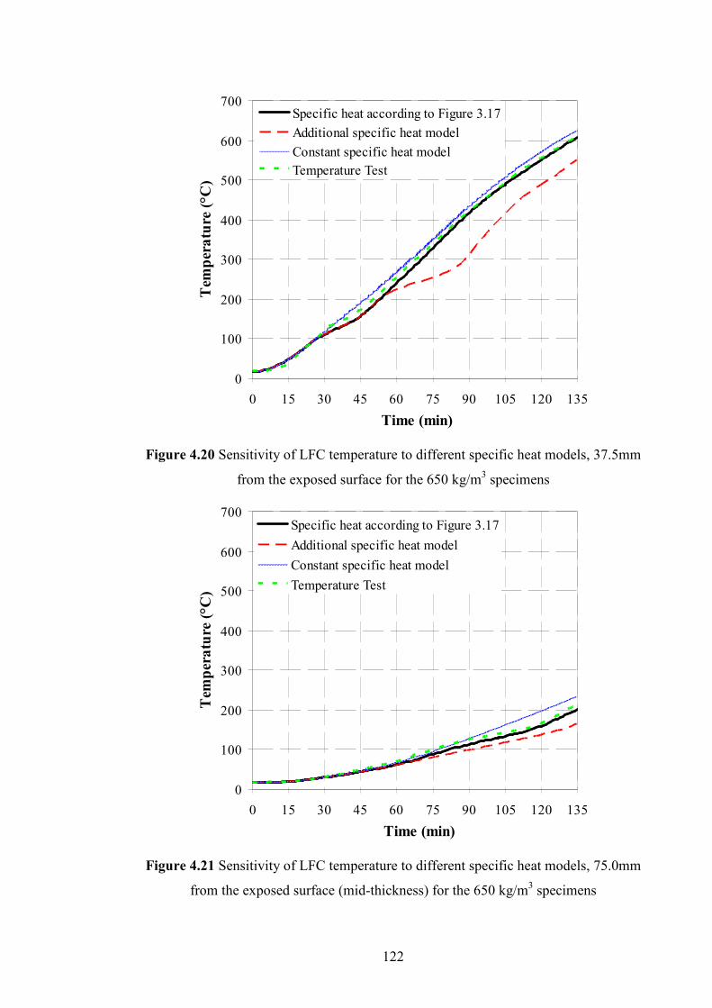
122
0
100
200
300
400
500
600
700
0 15 30 45 60 75 90 105 120 135
Time (min)
Tem
per
atu
re (
°C)
Specific heat according to Figure 3.17Additional specific heat model
Constant specific heat modelTemperature Test
Figure 4.20 Sensitivity of LFC temperature to different specific heat models, 37.5mm
from the exposed surface for the 650 kg/m3 specimens
0
100
200
300
400
500
600
700
0 15 30 45 60 75 90 105 120 135
Time (min)
Tem
per
atu
re (
°C)
Specific heat according to Figure 3.17
Additional specific heat model
Constant specific heat model
Temperature Test
Figure 4.21 Sensitivity of LFC temperature to different specific heat models, 75.0mm
from the exposed surface (mid-thickness) for the 650 kg/m3 specimens

123
0
100
200
300
400
500
600
700
0 15 30 45 60 75 90 105 120 135
Time (min)
Tem
per
atu
re (
°C)
Specific heat according to Figure 3.17
Additional specific heat model
Constant specific heat model
Temperature Test
Figure 4.22 Sensitivity of LFC temperature to different specific heat models, 112.5mm
from the exposed surface for the 650 kg/m3 specimens
0
100
200
300
400
500
600
700
0 15 30 45 60 75 90 105 120 135
Time (min)
Tem
per
atu
re (
°C)
Specific heat according to Figure 3.17
Additional specific heat model
Constant specific heat model
Temperature Test
Figure 4.23 Sensitivity of LFC temperature to different specific heat models at the
unexposed surface for the 650 kg/m3 specimens

124
4.5.2 Thermal conductivity-temperature model
The proposed analytical thermal conductivity model will be used and the sensitivity
study will focus on the pore size for the thermal conductivity model. For the 650 kg/m3
density, an average pore size of 0.72 mm is found appropriate from an analysis of the
internal structure of the sample shown in Figure 3.14 (Chapter 3). In the sensitivity
study, the pore size was changed to 0.4 mm and 1.0 mm.
Figure 4.24 shows the LFC thermal conductivity-temperature relationships for different
values of pore size. Figures 4.25-4.28 compare the predicted LFC temperatures at
different distance from the exposed surface using these thermal conductivity curves and
between the prediction results and the measured results. It is clear that the LFC
temperatures are moderately sensitive to the pore size. However, because thermal
conductivity deals with progressive heat transfer throughout the thickness, the
difference in results becomes proportionally much greater at positions further away
from the exposed surface. It is therefore important to obtain a sufficiently accurate
value for the pore size. For LFC, as shown in Figure 3.14, although there are variations
in the pore size for each density, these sizes may still considered to be relatively
uniform so an average value of pore size may be used. The results of this study, by
using the average pore size of 0.72mm, have been found to be acceptable.
0.00
0.10
0.20
0.30
0.40
0.50
0 200 400 600 800 1000
Temperature (°C)
Th
erm
al
Co
nd
ucti
vit
y (
W/m
°C).
. Proposed model with 0.72mm void size
Model with 0.40mm void size
Model with 1.00mm void size
Figure 4.24 Comparison of LFC thermal conductivity using different pore sizes
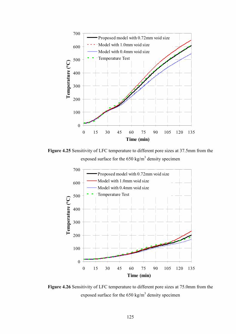
125
0
100
200
300
400
500
600
700
0 15 30 45 60 75 90 105 120 135
Time (min)
Tem
per
atu
re (
°C)
Proposed model with 0.72mm void size
Model with 1.0mm void size
Model with 0.4mm void size
Temperature Test
Figure 4.25 Sensitivity of LFC temperature to different pore sizes at 37.5mm from the
exposed surface for the 650 kg/m3 density specimen
0
100
200
300
400
500
600
700
0 15 30 45 60 75 90 105 120 135
Time (min)
Tem
per
atu
re (
°C)
Proposed model with 0.72mm void size
Model with 1.0mm void size
Model with 0.4mm void size
Temperature Test
Figure 4.26 Sensitivity of LFC temperature to different pore sizes at 75.0mm from the
exposed surface for the 650 kg/m3 density specimen

126
0
100
200
300
400
500
600
700
0 15 30 45 60 75 90 105 120 135
Time (min)
Tem
per
atu
re (
°C)
Proposed model with 0.72mm void size
Model with 1.0mm void size
Model with 0.4mm void sizeTemperature Test
Figure 4.27 Sensitivity of LFC temperature to different pore sizes at 112.5mm from the
exposed surface for the 650 kg/m3 density specimen
0
100
200
300
400
500
600
700
0 15 30 45 60 75 90 105 120 135
Time (min)
Tem
per
atu
re (
°C)
Proposed model with 0.72mm void size
Model with 1.0mm void size
Model with 0.4mm void size
Temperature Test
Figure 4.28 Sensitivity of LFC temperature to different pore sizes at the exposed
surface for the 650 kg/m3 density specimen
127
4.6 CO�CLUSIO�S
This chapter has presented the basis of the one-dimensional heat transfer modelling, the
implementation of the method and the validation of thermal properties model of LFC
panel. The comparison of test results with the numerical heat transfer analysis results
using the proposed thermal property models is close, confirming the validity of the
thermal conductivity models. Despite simplicity, the aforementioned analytical models
for specific heat and thermal conductivity of LFC of different densities give accurate
results. The superiority of the analytical model over the HGP test is that LFC of
different densities may be now considered without relying on extensive tests. The
prediction results are moderately affected by the air pore diameter. This suggests that
the air pore size should be determined with accuracy, but the average pore diameter will
be satisfactorily accurate. For LFC densities of 650 kg/m3 and 1000 kg/m3, the average
pore diameter may be taken as 0.72mm and 0.55mm respectively. The proposed model
is straightforward yet proficient and can be exploited to assist manufacturers to develop
their products without having to carry out numerous large-scale fire tests in the future.

128
CCHHAAPPTTEERR 55
EEXXPPEERRIIMMEE��TTAALL SSTTUUDDIIEESS OOFF MMEECCHHAA��II CCAALL
PPRROOPPEERRTTIIEESS OOFF LLFFCC EEXXPPOOSSEEDD TTOO EELLEEVVAATTEEDD
TTEEMMPPEERRAATTUURREESS
5.1 I�TRODUCTIO�
Even though LFC has low mechanical properties compared to normal weight concrete
(NSC), there is a potential of using this material as partition or load-bearing wall in
low-rise residential construction. Before it can be considered for use as a load-bearing
element in the building industry, it is necessary to acquire reliable information of its
mechanical properties at ambient and elevated temperatures for quantification of its fire
resistance performance. This chapter will present the results of experiments that have
been carried out to examine and characterize the mechanical properties of LFC at
elevated temperatures. Chapter 6 will present analytical models based on these
experimental results.
A variety of test methods may be used to obtain different aspects of mechanical
properties of materials at high temperatures, including the stressed test, the unstressed
test, and the unstressed residual strength test (Phan and Carino, 2003). In this research,
the unstressed test method was adopted for convenience. In the unstressed test, the
sample was heated, without preload, at a steady rate to the predetermined temperature.
While maintaining the target temperature, load was applied at a prescribed rate until
sample failure. Because the temperature is unchanged, the test is also referred to as
steady state test, as opposed to transient test in which the specimen temperature
changes with time.
LFC with 650 kg/m3 and 1000 kg/m3 density were cast and tested. The details of the
constituent material are shown in Table 2.6 (Chapter 2). The tests were carried out at

129
ambient temperature, 100, 200, 300, 400, 500, and 600°C. Compressive and three point
bending tests were carried out.
5.2 POROSITY MEASUREME�TS A�D PORE SIZE
The pore structure of cementitious material, determined by its porosity, is a very
significant characteristic as it influences the properties of the material such as strength
and durability. The porosity could therefore be a major factor influencing the material
properties of LFC and an in-depth look into this aspect is essential to determine the
relationships between porosity and material properties. Generally, the mechanical
properties of LFC decrease with increasing porosity. The density of LFC may be
diverse for the same water-cement ratio, through the integration of different amounts of
foam, which may result in a different porosity and void sizes. For that reason, any
change in the micro structure of LFC due to a variation in the void system may
influence the mechanical properties considerably in relation to density.
Therefore, before the mechanical property tests were carried out, the porosity of LFC at
elevated temperatures was measured according to the method described in Section
3.4.2. Table 5.1 indicates that replicate samples gave consistent results.
Table 5.1 Porosity of LFC obtained through Vacuum Saturation for mechanical
properties test
Porosity (%) Density
(kg/m3) Sample
Ambient 200°C 400°C 600°C
1/1 74.8 74.9 75.9 76.3
1/2 74.7 74.9 75.7 76.1 650
1/3 74.8 75.0 76.1 76.5
1/4 49.7 49.9 52.4 53.4
1/5 50.0 50.4 52.5 53.7 1000
1/6 50.4 50.7 52.9 54.1
130
5.2.1 Effect of high temperature on porosity of LFC
Usually, the porosity of cement based material changes when the temperature increases.
These changes in porosity can be characterized by considering phase changes in the
concrete at different temperatures. Kalifa et al. (1998) in their research credited the
increase in porosity with temperature to the release of chemically bound water and to
the microcracking produced by expansion of the cement paste. Gallé and Sercombe
(1999) attributed the growth of porosity to the formation of large capillary pores in the
concrete which corresponds to the release of adsorbed water in capillary pores and
release of chemically bound water in the hydrated cement paste. Gallé and Sercombe
(1999) observed that macropores correlated to microcracks observed at the surface of
specimens heated beyond 250°C. During the heating process, the authors observed
from 300°C a number of cracks on the LFC specimens due to the heating, which could
be concurrent with the growth of porosity and microstructural changes. Noumowé et al.
(1996) confirmed by mercury intrusion porosimetry an increment in the pore sizes of
concrete above temperature of 120 °C. Ye et al. (2007) attributed increase in porosity
due to the decomposition of C–S–H and CH (main hydration products). These
transformations formed additional void spaces in heated concrete.
Figure 5.1 presented the total porosity for each mix as a function of the temperature.
LFC of both densities experienced a slight monotonous increase in porosity with
temperature. The initial porosity for 650 and 1000 kg/m3 density is 74.8% and 50.0%
respectively. Between 200°C and 300°C, the porosity increased considerably for the
higher density LFC while the increase was more moderate for the lower density LFC
due to decomposition of the different amounts of calcium silicate hydrate gel and
sulfoaluminate. At 300°C, the measured porosity for 650 kg/m3 and 1000 kg/m3 density
is 75.5% and 51.9% correspondingly. For temperatures beyond 400°C, the measured
porosity showed some increase corresponding to the decomposition of calcium
hydroxide to form calcium oxide. At 600°C, the porosity is 76.3% and 53.7% for 650
and 1000 kg/m3 respectively. Nevertheless, in general, due to the high porosity at
ambient temperature, LFC may be considered to have almost constant porosity at
different temperatures.

131
The pore size of LFC determined through image analysis tool presented in Section 3.4.3
of this thesis illustrate images of the internal structure of the 650 and 1000 kg/m3
density LFC at ambient temperature which obviously demonstrates that the void sizes
are not uniform and the average void size is primarily a function of the LFC density.
The same analysis of the images was also done for both densities after being exposed to
high temperatures and the results indicate that the void size did not change much from
that at ambient temperature.
40
50
60
70
80
90
100
0 100 200 300 400 500 600Temperature (°C)
Po
rosi
ty (
%)
650 kg/m3
1000 kg/m3
`
Figure 5.1 Porosity of LFC of two initial densities as a function of temperature
5.3 COMPRESSIVE TESTS
5.3.1 Heating of specimens
Two different electric furnaces were used for heating the LFC specimens to the various
steady-state temperatures. One furnace had a maximum operating temperature of 450°C
(low temperature furnace), and the second furnace had a maximum operating
temperature of 1000°C (high temperature furnace). Each of the furnaces was capable of
holding three specimens. The low temperature furnace had a temperature range of 50°C
132
to 450°C and was used for four of the reported thermal exposure conditions: 100°C,
200°C, 300°C and 400°C.
The furnace temperature exposure profiles were produced by a programmable
microprocessor temperature controller attached to the furnace power supply and
monitored by a Type K thermocouple located in the furnace chamber. The high
temperature furnace (Figure 5.2) had a maximum operating temperature of 1000°C.
This furnace was used for exposing concrete specimens to 500°C and 600°C. This
furnace was also controlled by a programmable microprocessor temperature controller
attached to the furnace power supply based on feed-back temperature reading from a
Type K thermocouple located in the furnace chamber. Pre-testing checking of the
furnaces showed that both furnace controllers and furnace power system could maintain
furnace operating temperatures within ±1°C over the test range.

133
Figure 5.2 High temperature electric furnace with specimens
5.3.2 Test Set-up
The compressive tests were carried out on 100 x 200 mm cylinders. The specimens
were removed from moulds after 24 hours of casting and then cured in a water tank at
20 ± 2°C for 28 days. Prior to testing, the specimens were removed from the curing

134
tank and put in the oven for 24 hours at 105°C. After 24 hours, all the specimens were
removed from the oven and their ends were ground flat. To monitor the strain
behaviour at ambient temperature during loading, two strain gauges was fitted on each
sample for the ambient test only. These ambient temperature strain measurements were
used to confirm that the strain calculated based on the displacement of the loading
platen was of sufficient accuracy. Since it was difficult to measure strain at elevated
temperatures, the displacement of the loading platen was used to calculate the strain for
the elevated temperature tests. Four Type K thermocouples were installed in the central
plane of each cylinder specimen to measure the specimen temperature, as shown in
Figure 5.3.
Figure 5.3 Typical 100 x 200 mm cylinder specimen with thermocouples arrangement
Loading was applied using an ambient temperature machine after removing the test
samples from the furnace. Each specimen was wrapped with insulation sheets
immediately after being removed from the electric furnace to minimise heat loss from
the specimen to atmosphere. For each set, three replicate tests were carried out to check
consistency of results. The target temperatures were 20°C (room temperature), 100,
200, 300, 400, 500, and 600°C.

135
During the loading process, the temperature of each sample (thermocouple T3) was
measured and it was found that the temperature was stable throughout the testing
period. Figures 5.4 shows typical temperature variations throughout the loading phase
for specimens of 1000 kg/m3 density. As can be seen, because the duration of loading
was short (just over one minute), there was very little heat loss and the temperature
change was less than 0.5oC.
197
198
199
200
201
202
203
0 10 20 30 40 50 60 70 80Time (second)
Tem
per
atu
re (
°C)
Specimen 1
Specimen 2
Specimen 3
Figure 5.4 Temperature change during test of specimens of 1000 kg/m3 density at
target temperature of 200°C
5.3.3 Results and discussion
The compressive tests have yielded the following mechanical properties: compressive
strength, compressive stress-strain relationship, modulus of elasticity in compression
and failure mode in compression.
5.3.3.1 Effects of high temperature on compressive strength of LFC
As will be shown later in Section 5.3.3.2, the three duplicate tests of each series gave
very consistent results so the average results may be used. As expected, for both
densities, the LFC compressive strength decreased with temperature. Figures 5.5 and
5.6 present the compressive strength and normalized compressive strength of LFC at
different temperatures. On initial heating, the LFC made with Portland cement CEM1

136
lost the absorbed, evaporable (or free) water and then the chemically bound water. The
loss of water would induce micro cracking resulting in some reduction in strength.
Between 90°C to 170°C, the compressive strength decreased slowly due to the release
of free water and some of the chemically bound water. At this point, the reduction in
concrete strength is not significant and the compressive strength of the LFC samples at
200°C still retained about 94% of the original unheated value. Between 200 °C and
400°C, decomposition of C-S-H gel and the sulfoaluminate phases caused cracks in the
specimens (Taylor, 1992). These cracks had significant effects on the compressive
strength of LFC (Ai et al., 2001). At 400 °C, the LFC strength retained only about 75%
of its initial value for both densities. Further degradation and loss of strength continued
to take place at high temperatures. At temperature of 600°C, the LFC retained only
about 40% of the original strength for both densities. It should be pointed out that in
this test, thermal shock should not be a problem. The specimens were heated slowly
and no thermal crack was noticed before mechanical testing.
Since the compositions of both densities of LFC are identical, except for increased
pores in the lower density LFC, it is not surprising that the normalised strength –
temperature relationships of LFC of both densities are almost the same.
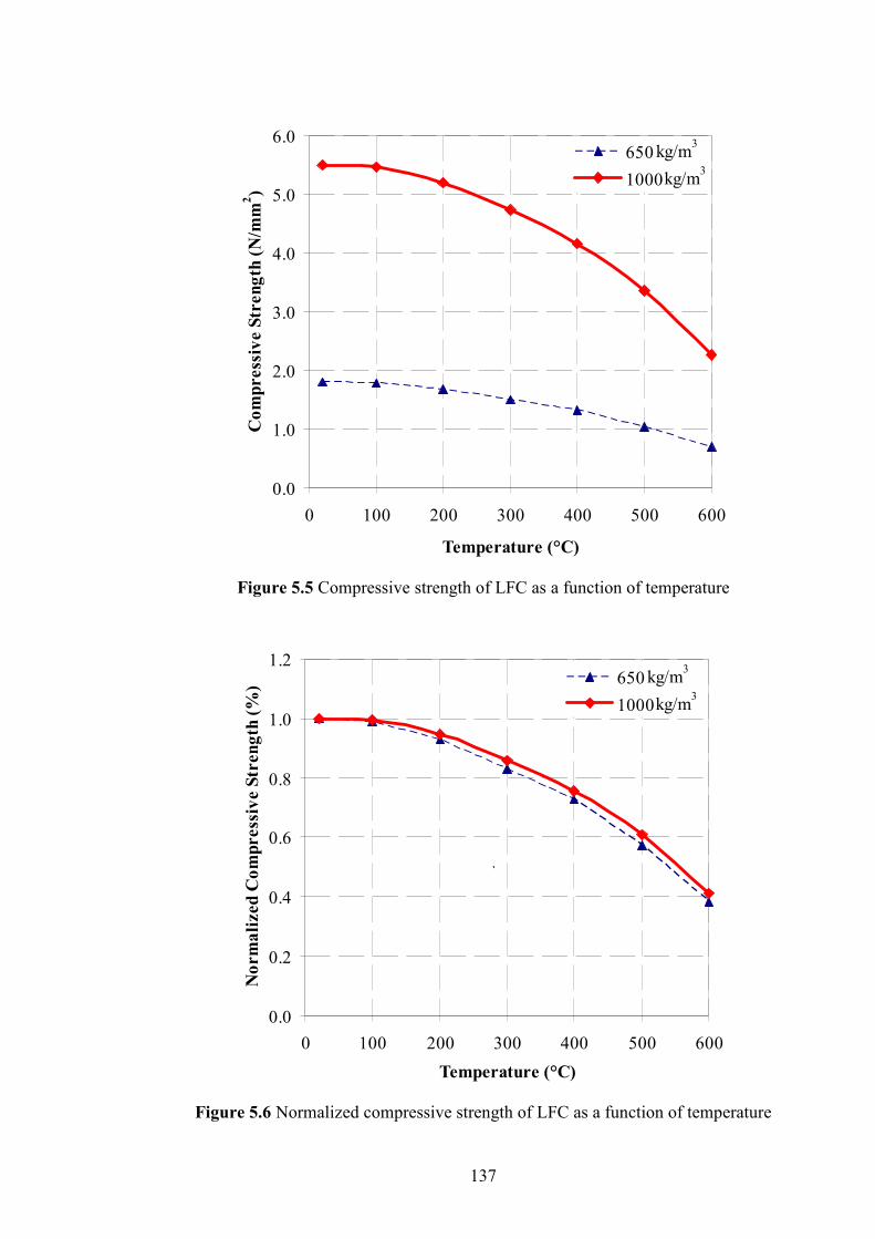
137
0.0
1.0
2.0
3.0
4.0
5.0
6.0
0 100 200 300 400 500 600
Temperature (°C)
Co
mp
ress
ive S
tren
gth
(�
/mm
2)
650
1000
kg/m3
kg/m3
Figure 5.5 Compressive strength of LFC as a function of temperature
0.0
0.2
0.4
0.6
0.8
1.0
1.2
0 100 200 300 400 500 600
Temperature (°C)
�o
rm
ali
zed
Co
mp
ress
ive S
tren
gth
(%
)
650
1000
`
kg/m3
kg/m3
Figure 5.6 Normalized compressive strength of LFC as a function of temperature
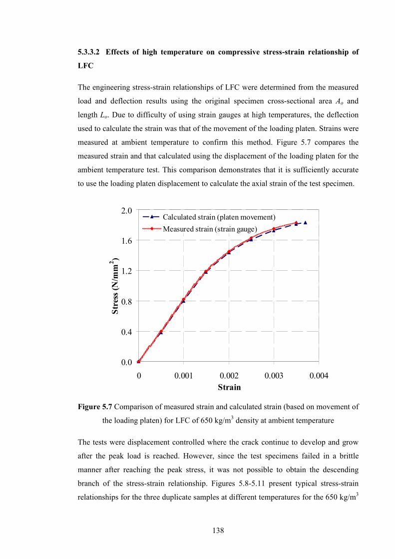
138
5.3.3.2 Effects of high temperature on compressive stress-strain relationship of
LFC
The engineering stress-strain relationships of LFC were determined from the measured
load and deflection results using the original specimen cross-sectional area Ao and
length Lo. Due to difficulty of using strain gauges at high temperatures, the deflection
used to calculate the strain was that of the movement of the loading platen. Strains were
measured at ambient temperature to confirm this method. Figure 5.7 compares the
measured strain and that calculated using the displacement of the loading platen for the
ambient temperature test. This comparison demonstrates that it is sufficiently accurate
to use the loading platen displacement to calculate the axial strain of the test specimen.
0.0
0.4
0.8
1.2
1.6
2.0
0 0.001 0.002 0.003 0.004Strain
Str
ess
(�/m
m2)
Calculated strain (platen movement)
Measured strain (strain gauge)
Figure 5.7 Comparison of measured strain and calculated strain (based on movement of
the loading platen) for LFC of 650 kg/m3 density at ambient temperature
The tests were displacement controlled where the crack continue to develop and grow
after the peak load is reached. However, since the test specimens failed in a brittle
manner after reaching the peak stress, it was not possible to obtain the descending
branch of the stress-strain relationship. Figures 5.8-5.11 present typical stress-strain
relationships for the three duplicate samples at different temperatures for the 650 kg/m3
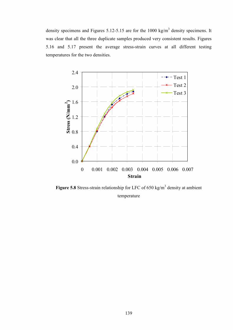
139
density specimens and Figures 5.12-5.15 are for the 1000 kg/m3 density specimens. It
was clear that all the three duplicate samples produced very consistent results. Figures
5.16 and 5.17 present the average stress-strain curves at all different testing
temperatures for the two densities.
0.0
0.4
0.8
1.2
1.6
2.0
2.4
0 0.001 0.002 0.003 0.004 0.005 0.006 0.007Strain
Str
ess
(�/m
m2)
Test 1
Test 2
Test 3
Figure 5.8 Stress-strain relationship for LFC of 650 kg/m3 density at ambient
temperature

140
0.0
0.4
0.8
1.2
1.6
2.0
2.4
0 0.001 0.002 0.003 0.004 0.005 0.006 0.007Strain
Str
ess
(�/m
m2)
Test 1
Test 2
Test 3
Figure 5.9 Stress-strain relationship for LFC of 650 kg/m3 density at 200°C
0.0
0.4
0.8
1.2
1.6
2.0
2.4
0 0.001 0.002 0.003 0.004 0.005 0.006 0.007Strain
Str
ess
(�/m
m2)
Test 1
Test 2
Test 3
Figure 5.10 Stress-strain relationship for LFC of 650 kg/m3 density at 400°C

141
0.0
0.4
0.8
1.2
1.6
2.0
2.4
0 0.001 0.002 0.003 0.004 0.005 0.006 0.007Strain
Str
ess
(�/m
m2)
Test 1
Test 2
Test 3
Figure 5.11 Stress-strain relationship for LFC of 650 kg/m3 density at 600°C
0.0
1.0
2.0
3.0
4.0
5.0
6.0
0 0.001 0.002 0.003 0.004 0.005Strain
Str
ess
(�/m
m2)
Test 1
Test 2
Test 3
Figure 5.12 Stress-strain relationship for LFC of 1000 kg/m3 density at ambient
temperature

142
0.0
1.0
2.0
3.0
4.0
5.0
6.0
0 0.001 0.002 0.003 0.004 0.005Strain
Str
ess
(�/m
m2)
Test 1
Test 2
Test 3
Figure 5.13 Stress-strain relationship for LFC of 1000 kg/m3 density at 200°C
0.0
1.0
2.0
3.0
4.0
5.0
6.0
0 0.001 0.002 0.003 0.004 0.005Strain
Str
ess
(�/m
m2)
Test 1
Test 2
Test 3
Figure 5.14 Stress-strain relationship for LFC of 1000 kg/m3 density at 400°C

143
0.0
1.0
2.0
3.0
4.0
5.0
6.0
0 0.001 0.002 0.003 0.004 0.005Strain
Str
ess
(�/m
m2)
Test 1
Test 2
Test 3
Figure 5.15 Stress-strain relationship for LFC of 1000 kg/m3 density at 600°C
0.0
0.4
0.8
1.2
1.6
2.0
2.4
0 0.001 0.002 0.003 0.004 0.005 0.006 0.007Strain
Str
ess
(�/m
m2)
Ambient200 °C400 °C600 °C
Figure 5.16 Average stress-strain relationships for LFC of 650 kg/m3 density at
different temperatures

144
0.0
1.0
2.0
3.0
4.0
5.0
6.0
0 0.001 0.002 0.003 0.004 0.005Strain
Str
ess
(�/m
m2)
Ambient200 °C400 °C600 °C
Figure 5.17 Average stress-strain relationships for LFC of 1000 kg/m3 density at
different temperatures
For both densities at all temperature levels, the ascending branch was linear for stress
up to 75% of the peak strength. The strain corresponding to the peak strength increased
at increasing temperatures. For LFC of 650 kg/m3 density, the maximum strains were
0.0034, 0.0039, 0.0055 and 0.0066 at ambient temperature, 200°C, 400°C and 600°C
respectively; for the 1000 kg/m3 density, the corresponding values were 0.0024, 0.0029,
0.0039 and 0.0048 at ambient, 200°C, 400°C and 600°C respectively. The increase in
strain results from opening of cracks initiated by the heating at higher temperatures.
Table 5.2 shows, for both densities and all temperatures, the elastic strain at the
maximum stress, the maximum strain at the maximum stress and the ratio of these two
strains. It appears that an average constant ratio of about 1.78 may be used for all
cases.

145
Table 5.2 Elastic strain at the maximum stress, maximum strain at the maximum stress
and the ratio of these two strains for both densities at different temperatures
Density
(kg/m3)
Temperature
(°C)
Elastic strain
at maximum
stress
Maximum
strain at
maximum stress
Ratio of maximum
strain at peak stress
to elastic strain at
peak stress
Ambient 0.0019 0.0034 1.79
200 0.0022 0.0039 1.77
400 0.0030 0.0055 1.83 650
600 0.0037 0.0066 1.78
Ambient 0.0013 0.0024 1.85
200 0.0016 0.0029 1.81
400 0.0023 0.0039 1.70 1000
600 0.0028 0.0048 1.71
5.3.3.3 Effect of high temperature on modulus of elasticity of LFC in compression
Figures 5.18 and 5.19 demonstrate the changes in modulus of elasticity of LFC in
compression as a function of temperature. The modulus of elasticity was taken as the
secant modulus at the point where the material changed from elastic to plastic behavior
from the experimental compressive stress–strain curve. Compared to the reduction in
LFC strength, the reduction in elastic modulus is greater. Both figures show that the
loss in modulus of elasticity began immediately upon heating when the samples began
to dry. The modulus of elasticity at 200°C, 400°C and 600°C was respectively about
75%, 40% and 25% of the original value for both densities.
As with changes in normalised strengths of LFC of both densities at elevated
temperatures, the normalised modulus of elasticity of LFC of both densities at the same
temperature was almost the same.

146
0.0
0.5
1.0
1.5
2.0
2.5
3.0
3.5
0 100 200 300 400 500 600
Temperature (°C)
Co
mp
res
siv
e M
od
ulu
s (k
�/m
m2)
`
650 kg/m3
1000 kg/m3
Figure 5.18 Compressive modulus of LFC as a function of temperature
0.0
0.2
0.4
0.6
0.8
1.0
1.2
0 100 200 300 400 500 600Temperature (°C)
�o
rma
lize
d C
om
pre
ssiv
e M
od
ulu
s (%
) 650 kg/m3
1000 kg/m3
Figure 5.19 Normalized compressive modulus of LFC as a function of temperature

147
5.3.3.4 Effects of high temperature on LFC failure mode in compression
All the tested LFC specimens exhibited brittle failure at all temperatures levels, failing
soon after reaching their peak strength. For the LFC of 650 kg/m3 density, the end
portion of the failed specimens resembled ‘double cone pattern’ (Figure 5.20b) at the
top and bottom at 400°C. When exposed to temperature of 600 °C, the specimens
crumbed and failed in an irregular pattern as shown in Figure 5.20(c). For LFC of 1000
kg/m3 density, vertical cracks appeared in the broken specimens with double cone
pattern at top and bottom at 400°C (Figure 5.21b); at 600 °C, it experienced the same
mode of failure as the LFC of 650 kg/m3 density (Figure 5.21c).
(a) at ambient (b) at 400°C (c) at 600°C
Figure 5.20 Failure modes of LFC of 650 kg/m3 density at different temperatures
(a) at ambient (b) at 400°C (c) at 600°C
Figure 5.21 Failure modes of LFC of 1000 kg/m3 density at different temperatures

148
5.4 THREE POI�T BE�DI�G TEST
5.4.1 Test set-up
Three methods may be used to obtain the tensile strength of concrete: direct tensile test,
tensile splitting test or flexural (three point bending) test. For convenience in this study,
the three point bending test was carried out. The preparation of samples followed a
similar procedure as outlined above for the compression tests. The specimens were
rectangular parallelepipeds of height (h) 25 mm, width (w) 125 mm and length L (l)
350 mm. As illustrated in Figures 5.22 and 5.23, the specimen was simply supported
and was subjected to point load at the centre point. The length between the supports
was Ls = 200 mm, giving a Ls/h aspect ratio of 8 and sufficient to ensure predominance
of bending behaviour. The load-deflection was recorded for the evaluation of flexural
tensile strength.
Figure 5.22 Three point bending test set up and specimen dimensions

149
Based on the sketch in Figure 5.23 and assuming linear elastic behaviour, the maximum
flexural bending strength (fcr) is at the centre (point B) which is defined as:
2
2
2
3
64
1
bd
PLbdPLf cr =
= … (5.1)
where PL4
1 is the bending moment at point B and
6
2bdis the elastic modulus for
rectangular cross-section. The flexural strength becomes tensile strength only if the
material behaviour is linear until tensile failure.
The flexural modulus of elasticity may be calculated using the following equation:
ybd
PLEcr 3
3
4= … (5.2)
where y is the maximum deformation at the centre of the beam.
Figure 5.23 Simply supported specimen subjected to a concentrated load at mid span

150
5.4.2 Results and discussion
The bending tests have yielded the following mechanical properties: flexural tensile
strength and flexural tensile modulus.
5.4.2.1 Effects of high temperature on flexural tensile strength of LFC
Since LFC is a brittle material, the bending test was intended to give a measure of the
flexural tensile strength of the LFC. Figures 5.24 and 5.25 present the variation in
flexural tensile strength of LFC as a function of temperature. The reduction in flexural
tensile strength of LFC occurred predominantly after 90°C, regardless of the density of
LFC. Consistent with changes in the aforementioned other mechanical properties of
LFC, which indicates that the primary mechanism causing degradation is micro
cracking, which occurs as the free water and chemically bound water evaporates from
the porous body. When the chemical constitution of LFC started to break down
between 200°C and 300°C due to decomposition of the C-S-H and sulfoaluminate
phases (3CaO.Al2O3.CaSO4.12H2O and 3CaO.Al2O3.3CaSO4.31H), cracks formed and
there was a significant drop in tensile strength. At 400°C, the tensile strength was about
60% of the initial value for both densities. At 600°C, the flexural tensile strength
achieved was only about 40% and 45% for 650 kg/m3 and 1000 kg/m3 densities
respectively.
0.0
0.2
0.4
0.6
0.8
1.0
0 100 200 300 400 500 600
Temperature (°C)
Fle
xu
ral
Ten
sile
Str
en
gth
(�
/mm
2)
650 kg/m3
1000 kg/m3
Figure 5.24 Flexural tensile strength of LFC as a function of temperature

151
0.0
0.2
0.4
0.6
0.8
1.0
1.2
0 100 200 300 400 500 600
Temperature (°C)
�o
rm
ali
zed
Fle
xu
ral
Str
eng
th (
%)
650 kg/m3
1000 kg/m3
Figure 5.25 Normalized flexural tensile strength of LFC as a function of temperature
The normalized flexural tensile strength – temperature relationships for both densities
are almost the same, which is consistent with other observed properties.
5.4.2.2 Effects of temperature on flexural tensile modulus of LFC
Figures 5.26 and 5.27 illustrate the changes in flexural modulus of LFC as a function of
temperature and compare the flexural modulus with the compressive modulus obtained
from the cylinder tests. Although there are some differences, the compressive modulus
and flexural modulus values are very similar for both densities and at different
temperatures.

152
0.0
0.5
1.0
1.5
2.0
2.5
3.0
3.5
0 100 200 300 400 500 600
Temperature (°C)
Fle
xu
ra
l te
nsi
le m
od
ulu
s (k
�/m
m2)
`
650 kg/m3
1000 kg/m3
Figure 5.26 Flexural tensile modulus of LFC as a function of temperature
0.0
0.2
0.4
0.6
0.8
1.0
1.2
0 100 200 300 400 500 600
Temperature (°C)
�o
rm
ali
zed
co
mp
ress
ive a
nd
fle
xu
ra
l m
od
ulu
s (%
)
650 kg/m3 (compressive modulus)
1000 kg/m3 (compressive modulus)
650 kg/m3 (flexural modulus)
1000 kg/m3 (flexural modulus)
kg/m3
kg/m3
kg/m3
kg/m3
Figure 5.27 Comparison of normalized compressive modulus and flexural tensile
modulus of LFC as a function of temperature
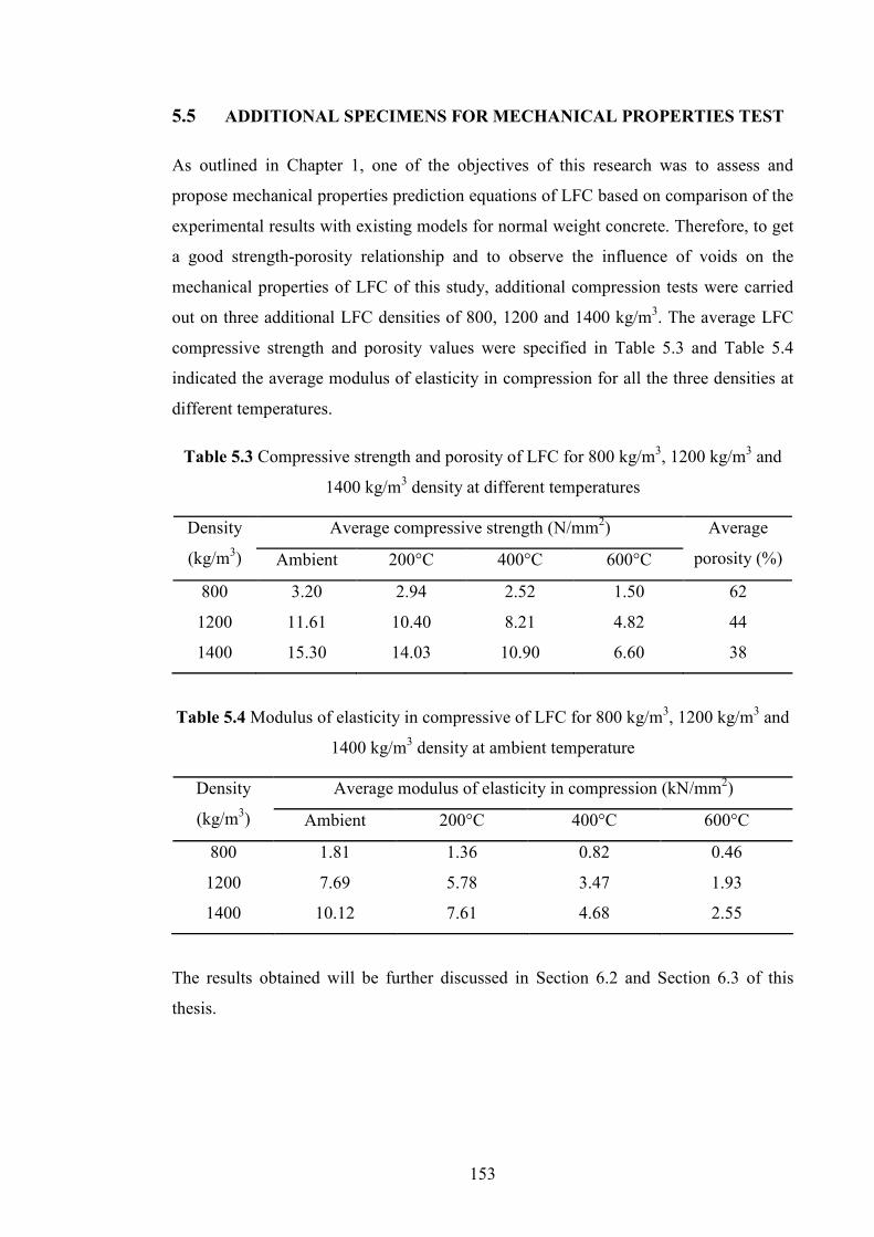
153
5.5 ADDITIO�AL SPECIME�S FOR MECHA�ICAL PROPERTIES TEST
As outlined in Chapter 1, one of the objectives of this research was to assess and
propose mechanical properties prediction equations of LFC based on comparison of the
experimental results with existing models for normal weight concrete. Therefore, to get
a good strength-porosity relationship and to observe the influence of voids on the
mechanical properties of LFC of this study, additional compression tests were carried
out on three additional LFC densities of 800, 1200 and 1400 kg/m3. The average LFC
compressive strength and porosity values were specified in Table 5.3 and Table 5.4
indicated the average modulus of elasticity in compression for all the three densities at
different temperatures.
Table 5.3 Compressive strength and porosity of LFC for 800 kg/m3, 1200 kg/m3 and
1400 kg/m3 density at different temperatures
Average compressive strength (N/mm2) Density
(kg/m3) Ambient 200°C 400°C 600°C
Average
porosity (%)
800 3.20 2.94 2.52 1.50 62
1200 11.61 10.40 8.21 4.82 44
1400 15.30 14.03 10.90 6.60 38
Table 5.4 Modulus of elasticity in compressive of LFC for 800 kg/m3, 1200 kg/m3 and
1400 kg/m3 density at ambient temperature
Average modulus of elasticity in compression (kN/mm2) Density
(kg/m3) Ambient 200°C 400°C 600°C
800 1.81 1.36 0.82 0.46
1200 7.69 5.78 3.47 1.93
1400 10.12 7.61 4.68 2.55
The results obtained will be further discussed in Section 6.2 and Section 6.3 of this
thesis.

154
5.6 CO�CLUSIO�S
This chapter has presented the results of an extensive series of experimental studies to
obtain compressive and tensile mechanical properties of LFC at elevated temperatures.
Compressive cylinder tests and three point bending tests were carried out for a range of
LFC densities at different temperatures from ambient up to 600oC. The mechanical
properties included compressive cylinder strength, compressive modulus of elasticity,
compressive stress-strain relationship, strain at the maximum compressive stress,
porosity, flexural bending strength and modulus of elasticity. The experimental results
consistently demonstrated that the loss in stiffness for cement based material like LFC
at elevated temperatures occurs predominantly after about 90°C, regardless of density.
This indicates that the primary mechanism causing stiffness degradation is
microcracking, which occurs as water expands and evaporates from the porous body.
As expected, reducing the density of LFC reduces its strength and stiffness. However,
for LFC of different densities, the normalised strength and stiffness (ratio of elevated
temperature value to ambient temperature value) – temperature relationships are very
similar. This chapter has principally focused on explanation of the experimental set-up
and presenting the experimental results of the mechanical properties of LFC at elevated
temperatures; Chapter 6 will present some quantitative information on the influence of
voids on the mechanical properties of LFC and comparison between the experimental
results and predictions of some existing predictive models based on normal weight
concrete.

155
CCHHAAPPTTEERR 66
MMEECCHHAA��II CCAALL PPRROOPPEERRTTYY PPRREEDDIICCTTIIVVEE MMOODDEELLSS FFOORR
LLFFCC EEXXPPOOSSEEDD TTOO EELLEEVVAATTEEDD TTEEMMPPEERRAATTUURREESS
6.1 MODELS FOR LFC MECHA�ICAL PROPERTIES
Since the LFC employed in this study used the same Portland Cement SEM1 as in
normal weight concrete for which a number of mechanical property models have been
developed, this chapter is intended to assess whether any of these models would be
suitable for LFC. A two-stage comparison will be made: assessment of models at
ambient temperature and assessment of models for elevated temperatures, based on
ambient temperature results.
The aim of this investigation is to propose a procedure to predict the mechanical
properties of LFC, based on existing mechanical property predictive models. This
procedure is expected to assist manufacturers and future researchers to develop
improved products with reduced cost of experimentation. Whilst full-scale tests to
regulatory standards will still be necessary for final accreditation purpose, much of this
may be avoided by developing a method to predict the mechanical properties of LFC at
ambient and elevated temperatures during the development stage.
6.2 PREDICTIO� OF MECHA�ICAL PROPERTIES OF LFC AT
AMBIE�T TEMPERATURE
For LFC at ambient temperature, porosity represents the most important factor in
affecting its strength. Hoff (1972) proposed a single strength-porosity model for
cellular concrete with cement paste by combining the space taken by evaporable water
and air-voids. Tam et al. (1987) reported a model for strength of LFC based on Feret’s
equations for a limited set of operating conditions. This equation was enhanced by

156
integrating the degree of hydration through Power’s gel-space ratio concept. Balshin
proposed an equation which provided a good fit to the plot of compressive strength
against porosity for slate based autoclaved aerated concretes (Watson, 1980), at all ages
of LFC made of cement paste containing high percentage of ash (Kearsley and
Wainwright, 2002) and LFC containing high amount of fly ash as replacement to sand
(Nambiar and Ramamurthy, 2008).
6.2.1 Strength-porosity relationship
Balshin (1949) strength-porosity relationship will be considered to assess the effects of
porosity on compressive strength of LFC, which may be expressed using the following
form:
n
cc ff )1(0, ε−= …..(6.1)
where fc is the compressive strength of LFC with porosity ε , fc,0 is the compressive
strength at zero porosity and n is a coefficient to be determined.
Figure 6.1 plots the recorded LFC compressive strength-porosity relationship for
different LFC densities at ambient temperature (results of compressive strength
presented in Table 5.3). Using Balshin’s strength-porosity relationship, the best
correlation is obtained with n=2.4, which was represented by the solid curve in Figure
6.1. A correlation coefficient of 0.914 indicates a good correlation between this model
and the test results. Thus, the compressive strength of LFC at ambient temperature can
be expressed as a power function of porosity as follow:
4.2)1(2.39 ε−=cf …..(6.2)

157
0
3
6
9
12
15
18
30 40 50 60 70 80Measured porosity (%)
Co
mp
ress
ive S
tren
gth
(�
/mm2
)
Figure 6.1 Compressive strength-porosity relation for LFC at ambient temperature
For interest, a similar study was carried out by others for LFC of different densities at
ambient temperature. From the experimental results of this study for LFC at different
temperatures, the same exercise was undertaken. The results are summarised in Table
6.1 and compared with results by others for other types of concrete. The n values of
LFC obtained in this study show some consistency, but are different from other
researchers. The n values of this study are much lower than from other studies,
indicating that the LFC of this study suffered less void induced loss of strength.

158
Table 6.1 Comparison of n-values in strength-porosity model for different concretes
Constants
Researchers Concrete type Mix composition fc.0
(N/mm2) n
Hoff (1972) LFC Cement paste 115-290 2.7-3.0
Narayanan and
Ramamurthy (2000)
Aerated concrete
(non autoclaved) Cement-sand 26.6 3.2
Kearsley and
Wainwright (2002) LFC
Cement with and
without fly ash 188 3.1
LFC (ambient) 39.2 2.4
LFC (200°C) 38.5 2.4
LFC (400°C) 28.1 2.4 Present work
LFC (600°C)
Cement-sand
19.5 2.6
6.2.2 Modulus of elasticity-porosity relationship
As acknowledged by the author, the strength-porosity relationship proposed by Balshin
(Equation 6.1) has so far only been used to determine the compressive strength of
porous material. This section will explore whether this equation (Equation 6.1) is also
appropriate to establish the modulus of elasticity-porosity relationship for LFC. In order
to do so, the experimental results of modulus of elasticity for all densities will be
plotted as a function of porosity.
Figure 6.2 shows the recorded LFC modulus of elasticity-porosity relationship for
different LFC densities at ambient temperature (results of modulus of elasticity in Table
5.4). Surprisingly, the same relationship can be used. The best correlation was found by
using n=2.8, shown by the solid curve in Figure 6.2. A correlation coefficient of 0.936
indicates strong relationship between the model and the test results. Thus, the following
modulus of elasticity-porosity relationship of LFC at ambient temperature is obtained:
8.2)1(9.32 ε−=cE …..(6.3)
where Ec is the compressive modulus of LFC at ambient temperature and ε is porosity.

159
0
2
4
6
8
10
12
30 40 50 60 70 80Measured porosity (%)
Co
mp
ress
ive M
od
ulu
s (k
�/m
m2)
Figure 6.2 Modulus of elasticity-porosity relation for LFC at ambient temperature
From the experimental results of this study for LFC at different temperatures, the same
exercise was undertaken to obtain the modulus of elasticity-porosity relationships. The
results were summarised in Table 6.2 which shows a constant n value at different
temperatures.
Table 6.2 Summary of Ec.0 and n values for modulus of elasticity-porosity relationship
at different temperatures according to Balshin’s model
Constants Temperature (°C)
Ec.0 (kN/mm2) n
Ambient 32.9 2.8
200 24.7 2.8
400 15.0 2.8
600 8.2 2.8

160
6.2.3 Modulus of elasticity-compressive strength relationship
As presented in the literature review chapter (Section 2.2.5), Jones and McCarthy
(2005) proposed a relationship linking the modulus of elasticity with the compressive
strength of LFC (Equation 2.3) at ambient temperature. Although Equation 2.3 is
considered applicable only for a minimum compressive strength of 5 N/mm2, Figure
6.3 showed that the same modulus of elasticity-compressive strength relationship exists
for LFC across the entire strength range.
0
2
4
6
8
10
12
0 2 4 6 8 10 12 14 16 18
Compressive Strength (�/mm2)
Mo
du
lus
of
ela
stic
ity
(k
�/m
m2)
Predicted results (Eq. 2.3)
Average test results
Figure 6.3 Modulus of elasticity-compressive strength relation for LFC at ambient
temperature
6.2.4 Porosity-density relationship
Through using Equation 6.2 and Equation 6.3, it was possible to obtain an accurate
assessment of the compressive strength and modulus of elasticity of LFC. Nevertheless,
these models require input of the porosity value. Unfortunately, porosity was a property
not frequently measured outside the laboratory, and therefore it is necessary to provide
a model to obtain the porosity. The simplest method to calculate the porosity value was
to relate it to LFC density. Since the pores inside LFC were created due to addition of

161
foams, by knowing the solid density of cement paste (without foam), one can easily
predict the porosity of LFC of any other density using the following equation:
sc
drysc
ρ
ρρε
−= ….. (6.4)
where ε is the porosity, ρsc is the solid density of cement paste (without foam) and ρdry
is the dry density of LFC.
The accuracy of Equation 6.4 was checked by comparing the porosity values calculated
using Equation 6.4 and the measured porosity values using the Vacuum Saturation
Apparatus for different LFC densities, as shown in Figure 6.4. It should be noted that
an average solid density of cement paste (ρsc) of 2100 kg/m3 was established through
the experiment. The agreement is excellent.
0
20
40
60
80
100
600 700 800 900 1000 1100 1200 1300 1400 1500
Density (kg/m3)
Po
rosi
ty (
%)
Measured Porosity
Predicted Porosity
Figure 6.4 Comparison of predicted porosity with measured porosity as a function of
density

162
6.3 PREDICTIO� OF MECHA�ICAL PROPERTIES OF LFC AT
ELEVATED TEMPERATURES
As outlined in Section 2.4.2, a number of concrete mechanical property models have
been proposed by others for normal weight concrete. This section was intended to
assess the applicability of these models to LFC.
6.3.1 Compressive strength models for concrete at elevated temperatures
Several models have been proposed to estimate concrete compressive strength at high
temperatures.
Li and Purkiss (2005) presented a review of the available models for the mechanical
behaviour of concrete at elevated temperatures and provided comparisons between the
existing models. Li and Purkiss (2005) suggested the following model to predict the
compressive strength of concrete at elevated temperatures:
+
⋅+
⋅−
⋅⋅= 002.1100
025.0100
03.0100
00165.023
TTTff ccT …..(6.5)
where fcT is the concrete compressive strength at elevated temperature, fc is the concrete
compressive strength at ambient temperature and T is temperature in oC.
The Eurocode 2 (2004) model is given below:
ccT ff = CT °≤ 100 …..(6.6a)
)00067.0067.1( Tff ccT ⋅−⋅= CTC °≤≤° 400100 …..(6.6b)
)0016.044.1( Tff ccT ⋅−⋅= CT °≥ 400 …..(6.6c)
Hertz (2005) in his study on concrete strength for fire safety design had derived an
idealised data for the compressive strength of a number of concretes which included
test series from more than 400 test comprising approximately 3000 specimens. The data
covered a range of concretes with aggregates such as siliceous materials, limestone,
granite, sea gravel, pumice, and expanded clay. He then proposed a model for

163
compressive strength of concrete at elevated temperatures that allowed for different
types of aggregate to be differentiated as follows:
+
+
++
⋅=64
64
8
8
2
21
1
1
T
T
T
T
T
T
T
Tff ccT …..(6.7)
Assuming LFC as a type of lightweight aggregate concrete for application of Hertz’s
model, then T1=100,000, T2=1100, T8=800 and T64=940.
Figures 6.5 to 6.9 compare predictions of the above-mentioned models for all LFC
densities at different temperatures against the experimental results from this study. As
expected, the results showed that the Hertz (2005) model gave much higher results than
the test results and was not appropriate for LFC. Both the Eurocode 2 (2004) and Li and
Purkiss (2005) models seem to give good results and be suitable for LFC, with the
Eurocode 2 predictions being slightly higher than the measured values.

164
0.0
0.2
0.4
0.6
0.8
1.0
1.2
0 100 200 300 400 500 600
Temperature (°C)
�o
rm
ali
zed
co
mp
ress
ive s
tren
gth
Eurocode 2
Li and Purkiss
Hertz
Average test results
Figure 6.5 Comparison of normalized compressive strength-temperature relationships
for 650 kg/m3
0.0
0.2
0.4
0.6
0.8
1.0
1.2
0 100 200 300 400 500 600
Temperature (°C)
�o
rm
ali
zed
co
mp
ress
ive s
tren
gth
Eurocode 2
Li and Purkiss
Hertz
Average test results
Figure 6.6 Comparison of normalized compressive strength-temperature relationships
for 800 kg/m3
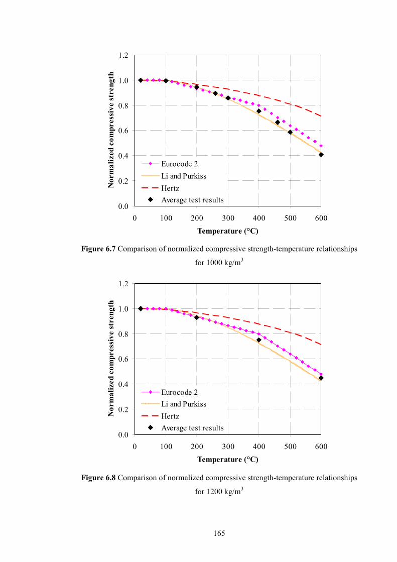
165
0.0
0.2
0.4
0.6
0.8
1.0
1.2
0 100 200 300 400 500 600
Temperature (°C)
�o
rm
ali
zed
co
mp
ress
ive s
tren
gth
Eurocode 2
Li and Purkiss
Hertz
Average test results
Figure 6.7 Comparison of normalized compressive strength-temperature relationships
for 1000 kg/m3
0.0
0.2
0.4
0.6
0.8
1.0
1.2
0 100 200 300 400 500 600
Temperature (°C)
�o
rm
ali
zed
co
mp
ress
ive s
tren
gth
Eurocode 2
Li and Purkiss
Hertz
Average test results
Figure 6.8 Comparison of normalized compressive strength-temperature relationships
for 1200 kg/m3

166
0.0
0.2
0.4
0.6
0.8
1.0
1.2
0 100 200 300 400 500 600
Temperature (°C)
�o
rm
ali
zed
co
mp
ress
ive s
tren
gth
Eurocode 2
Li and Purkiss
Hertz
Average test results
`
Figure 6.9 Comparison of normalized compressive strength-temperature relationships
for 1400 kg/m3
6.3.2 Models for modulus of elasticity of concrete at elevated temperatures
The elastic modulus of concrete would be affected primarily by the same factors
influencing its compressive strength (Malhotra, 1982). Due to different definitions of
modulus of elasticity and the difficulty of precisely calculating this value, it was not
surprising that previous researchers have revealed great disparity in the experimental
results. In this research, the modulus of elasticity was calculated as the secant modulus
corresponding to 0.75 ultimate stress. The following models were considered.
Lu (1989), in his study on fire response of reinforced concrete beams, performed an
unstressed test procedure to establish the modulus of elasticity of concrete when
exposed to high temperatures. He proposed the following tri-linear expression between
EcT and T:
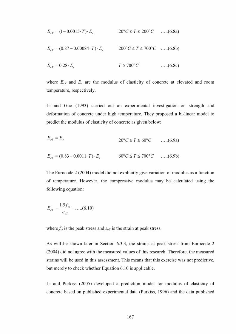
167
ccT ETE ⋅⋅−= )0015.01( CTC °≤≤° 20020 …..(6.8a)
ccT ETE ⋅⋅−= )00084.087.0( CTC °≤≤° 700200 …..(6.8b)
ccT EE ⋅= 28.0 CT °≥ 700 …..(6.8c)
where EcT and Ec are the modulus of elasticity of concrete at elevated and room
temperature, respectively.
Li and Guo (1993) carried out an experimental investigation on strength and
deformation of concrete under high temperature. They proposed a bi-linear model to
predict the modulus of elasticity of concrete as given below:
ccT EE = CTC °≤≤° 6020 …..(6.9a)
ccT ETE ⋅⋅−= )0011.083.0( CTC °≤≤° 70060 …..(6.9b)
The Eurocode 2 (2004) model did not explicitly give variation of modulus as a function
of temperature. However, the compressive modulus may be calculated using the
following equation:
oT
cT
cT
fE
ε5.1
= …..(6.10)
where fct is the peak stress and εoT is the strain at peak stress.
As will be shown later in Section 6.3.3, the strains at peak stress from Eurocode 2
(2004) did not agree with the measured values of this research. Therefore, the measured
strains will be used in this assessment. This means that this exercise was not predictive,
but merely to check whether Equation 6.10 is applicable.
Li and Purkiss (2005) developed a prediction model for modulus of elasticity of
concrete based on published experimental data (Purkiss, 1996) and the data published

168
in Eurocode 2 (2004). They defined the elastic modulus as the initial tangent modulus
and gave the following relationships:
ccT EE = CT °≤ 60 …..(6.11a)
ccT ET
E ⋅−
=740
800 CTC °≤≤° 80060 …..(6.11b)
Khennane and Baker (1993) in their research on concrete behavior under variable
temperature and stress presented a plasticity model using a strain-rate formulation to
depict the uniaxial response of concrete when subjected to combined thermal and
mechanical actions and they proposed the following equation:
ccT ETE ⋅+⋅−= )025641.1001282.0( CTC °≤≤° 80020 …..(6.12)
Figures 6.10 to 6.14 compare predictions of the various models with the test results for
all densities at different temperatures. Except for the Lu (1989) and the Li and Guo
(1993) models, all the other models give good predictions of the test results,
particularly considering the relatively wide scatter of experimental results reported in
literature. In conjunction with the conclusion drawn in the last section for compressive
strength, both the Eurocode 2 (2004) and the Li and Purkiss (2005) models may be
used. However, as previously mentioned, using the equation of Eurocode 2 (2004) was
predicated on the assumption that an independent means of obtaining the strains at peak
stresses can be established.

169
0.0
0.2
0.4
0.6
0.8
1.0
1.2
0 100 200 300 400 500 600
Temperature (°C)
�o
rm
ali
zed
mo
du
lus
of
ela
stic
ity
Lu
Li and Guo
Li and Purkiss
Eurocode 2
Khennane and Baker
Average test results
Figure 6.10 Comparison of normalized elastic modulus-temperature relationships for
650 kg/m3
0.0
0.2
0.4
0.6
0.8
1.0
1.2
0 100 200 300 400 500 600
Temperature (°C)
�o
rm
ali
zed
mo
du
lus
of
ela
stic
ity
Lu
Li and Guo
Li and Purkiss
Eurocode 2
Khennane and Baker
Average test results
Figure 6.11 Comparison of normalized elastic modulus-temperature relationships for
800 kg/m3

170
0.0
0.2
0.4
0.6
0.8
1.0
1.2
0 100 200 300 400 500 600
Temperature (°C)
�o
rm
ali
zed
mo
du
lus
of
ela
stic
ity
Lu
Li and Guo
Li and Purkiss
Eurocode 2
Khennane and Baker
Average test results
Figure 6.12 Comparison of normalized elastic modulus-temperature relationships for
1000 kg/m3
0.0
0.2
0.4
0.6
0.8
1.0
1.2
0 100 200 300 400 500 600
Temperature (°C)
�o
rm
ali
zed
mo
du
lus
of
ela
stic
ity
Lu
Li and Guo
Li and Purkiss
Eurocode 2
Khennane and Baker
Average test results
Figure 6.13 Comparison of normalized elastic modulus-temperature relationships for
1200 kg/m3

171
0.0
0.2
0.4
0.6
0.8
1.0
1.2
0 100 200 300 400 500 600
Temperature (°C)
�o
rm
ali
zed
mo
du
lus
of
ela
stic
ity
Lu
Li and Guo
Li and Purkiss
Eurocode 2
Khennane and Baker
Average test results
Figure 6.14 Comparison of normalized elastic modulus-temperature relationships for
1400 kg/m3
6.3.3 Strain at peak compressive stress
For predicting LFC strain at the maximum compressive stress ( oTε ), the following
models may be considered in regards to the models for cases where concrete specimens
were not loaded during the heating process.
i.) Anderberg and Thelandersson (1976)
002666.0)00000167.0( +⋅= ToTε CT °≤ 800 …..(6.13)
ii.) Khennane and Baker (1993)
003.0=oTε CTC °≤≤° 20020 …..(6.14a)
000686.0)00001156.0( +⋅= ToTε CT °≥ 200 …..(6.14b)

172
iii.) Bazant and Chern (1987)
00216.0)0000064.0( −⋅= ToTε CTC °≤≤° 60020 …..(6.15)
iv.) Li and Purkiss (2005)
284'
)20(109.0)20(1021.02
−⋅×−−⋅×+⋅
= −− TTE
f
c
c
oTε …..(6.16)
v.) Eurocode 2 (2004)
The Eurocode 2 relationship is reproduced in Table 6.3
Table 6.3 Temperature dependence of the strain at the peak stress
point (Eurocode 2, 2004)
Temperature (°C) Strain corresponding to peak stress
0 0.0025
100 0.0040
200 0.0055
300 0.0070
400 0.0100
500 0.0150
600 0.0250
700 0.0250
800 0.0250
900 0.0250
1000 0.0250
Figure 6.15 provides a comparison of the above-mentioned prediction models with the
average test results for the two densities at different temperatures. It was clear from
Figure 6.15 that the Eurocode 2 (2004) model appears to give the worst prediction. The
model of Li and Purkiss (2005) provides the upper bound for εoT and the model of
Anderberg and Thelandersson (1976) provided the lower bound. The results of the three

173
remaining models gave close agreement with the experimental results. Out of all the
models, the Bazant and Chern (1987) prediction appeared to give the best agreement
with these experimental results.
0.000
0.005
0.010
0.015
0.020
0.025
0.030
0 100 200 300 400 500 600
Temperature (°C)
Str
ain
at
pea
k s
tress
(ε
oT)
Li and Purkiss (650 kg/m3)Li and Purkiss (1000 kg/m3)Khennane and BakerBazant and ChernAnderberg and ThelandersonEurocode 2Average test results (650 kg/m3)Average test results (1000 kg/m3)
Figure 6.15 Comparison of strain at maximum stress-temperature relationships
Although the Eurocode 2 values of strain at peak stress cannot be used for LFC, the
Eurocode 2 equation (Equation 6.10) does reveal that the strain at peak stress is simply
1.5 times the elastic strain at peak stress. In fact, based on the experimental results of
this research, the strain at peak stress is about 1.78 times the elastic strain at peak stress.
For analysis of structural behaviour of LFC, it is more important to correctly predict the
modulus of elasticity than the strain at peak stress. Therefore, this research recommends
using the Li and Purkiss equation (Equation 6.11) to directly predict the modulus of
elasticity change as a function of temperature. Using the Eurocode 2 model (Equation
6.6) for prediction of LFC strength at different temperatures and applying the constant
ratio of 1.78 as obtained from this research, the variable LFC strain at peak stress for
different densities can be obtained as a function of temperature.

174
Figure 6.16 compares the calculated strain at peak stress values with measured strain at
peak stress values for both densities at different temperatures. The agreement is
excellent.
0.0000
0.0025
0.0050
0.0075
0.0100
0.0125
0 100 200 300 400 500 600 700
Temperature (°C)
Str
ain
at
pea
k s
tres
s (
εo
T)
Calculated value (650 kg/m3)
Calculated value (1000 kg/m3)
Measured value (650 kg/m3)
Measured value (1000 kg/m3)
`
Figure 6.16 Comparison of calculated and measured strain at peak stress values for 650
and 1000 kg/m3 densities at different temperatures
6.3.4 Stress-strain relationship of concrete exposed to elevated temperatures
The three models which will be considered for the stress-strain relationship of LFC
were the Anderberg and Thelandersson (1976) model, Lie and Lin (1985) model and
the Eurocode 2 (2004) model.
i.) Anderberg and Thelandersson model (1976)
This model was based on transient tests and the ascending compressive part of the
relationship is:
⋅−⋅=
oT
cT
cTcTcT Efεε
ε2
2' …..(6.17)
where EcT is the modulus of elasticity of concrete at elevated temperature.

175
ii.) Lie and Lin model (1985)
This model includes an ascending and a descending branch. However, since only the
ascending branch of LFC stress-strain relationship could be obtained, only the
ascending branch equation will be given, which was as follows.
−−⋅=
2
' 1oT
cToT
cTcT ffεεε
oTcT εε ≤ …..(6.18)
where f’cT is the concrete compressive stress at elevated temperature, fcT is the concrete
compressive strength at elevated temperature, εcT is the concrete strain at elevated
temperature and εoT is the strain at the maximum concrete stress.
iii.) Eurocode 2 model (2004)
The Eurocode 2 equation is:
+
=3
'
2
3
oT
cT
oT
cTcTcT
ff
εε
ε
ε …(6.19)
All three models require input of the LFC peak stress (fcT) and strain at peak stress (εcT).
For this exercise, the measured values were used so that this comparison does suffer
from any inaccuracy in prediction of these input values.
Figures 6.17(a-d) and 6.18(a-d) compare predictions of the different models with the
average test results for the two densities at different temperatures (ambient, 200°C,
400°C and 600°C). It should be pointed out that when using the Eurocode 2 model
(Equation 6.19), the calculated strain at peak stress was used. Except for the Anderberg
and Thelandersson (1976) model, Lie and Lin (1985) and Eurocode 2 (2004) model
were almost identical and in good agreement with the experimental results for all
densities at different temperatures.

176
0.0
0.2
0.4
0.6
0.8
1.0
1.2
0 0.001 0.002 0.003 0.004 0.005 0.006 0.007
Strain
Str
ess
ra
tio
(f c
T/f
c)
Anderberg and Thelanderson
Lie and Lin
Eurocode 2
Average test results
Figure 6.17(a) Stress-strain curves for 650 kg/m3 density at ambient temperature
0.0
0.2
0.4
0.6
0.8
1.0
1.2
0 0.001 0.002 0.003 0.004 0.005 0.006 0.007
Strain
Str
ess
ra
tio
(f c
T/f
c)
Anderberg and Thelanderson
Lie and Lin
Eurocode 2
Average test results
Figure 6.17(b) Stress-strain curves for 650 kg/m3 density at 200°C

177
0.0
0.2
0.4
0.6
0.8
1.0
1.2
0 0.001 0.002 0.003 0.004 0.005 0.006 0.007
Strain
Str
ess
ra
tio
(f c
T/f
c)
Anderberg and Thelanderson
Lie and Lin
Eurocode 2
Average test results
Figure 6.17(c) Stress-strain curves for 650 kg/m3 density at 400°C
0.0
0.2
0.4
0.6
0.8
1.0
1.2
0 0.001 0.002 0.003 0.004 0.005 0.006 0.007
Strain
Str
ess
ra
tio
(f c
T/f
c)
Anderberg and Thelanderson
Lie and Lin
Eurocode 2
Average test results
Figure 6.17(d) Stress-strain curves for 650 kg/m3 density at 600°C
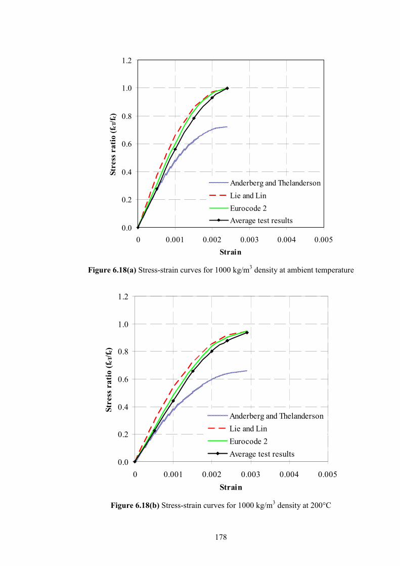
178
0.0
0.2
0.4
0.6
0.8
1.0
1.2
0 0.001 0.002 0.003 0.004 0.005
Strain
Str
ess
ra
tio
(f c
T/f
c)
Anderberg and Thelanderson
Lie and Lin
Eurocode 2
Average test results
Figure 6.18(a) Stress-strain curves for 1000 kg/m3 density at ambient temperature
0.0
0.2
0.4
0.6
0.8
1.0
1.2
0 0.001 0.002 0.003 0.004 0.005
Strain
Str
ess
ra
tio
(f c
T/f
c)
Anderberg and Thelanderson
Lie and Lin
Eurocode 2
Average test results
Figure 6.18(b) Stress-strain curves for 1000 kg/m3 density at 200°C

179
0.0
0.2
0.4
0.6
0.8
1.0
1.2
0 0.001 0.002 0.003 0.004 0.005
Strain
Str
ess
ra
tio
(f c
T/f
c)
Anderberg and Thelanderson
Lie and Lin
Eurocode 2
Average test results
Figure 6.18(c) Stress-strain curves for 1000 kg/m3 density at 400°C
0.0
0.2
0.4
0.6
0.8
1.0
1.2
0 0.001 0.002 0.003 0.004 0.005
Strain
Str
ess
ra
tio
(f c
T/f
c)
Anderberg and Thelanderson
Lie and Lin
Eurocode 2
Average test results
Figure 6.18(d) Stress-strain curves for 1000 kg/m3 density at 600°C
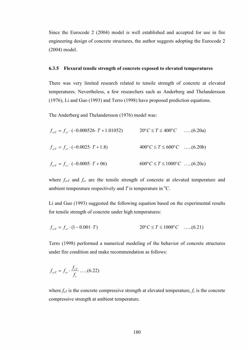
180
Since the Eurocode 2 (2004) model is well established and accepted for use in fire
engineering design of concrete structures, the author suggests adopting the Eurocode 2
(2004) model.
6.3.5 Flexural tensile strength of concrete exposed to elevated temperatures
There was very limited research related to tensile strength of concrete at elevated
temperatures. Nevertheless, a few researchers such as Anderberg and Thelandersson
(1976), Li and Guo (1993) and Terro (1998) have proposed prediction equations.
The Anderberg and Thelandersson (1976) model was:
)01052.1000526.0( +⋅−⋅= Tff crcrT CTC °≤≤° 40020 …..(6.20a)
)8.10025.0( +⋅−⋅= Tff crcrT CTC °≤≤° 600400 …..(6.20b)
)060005.0( +⋅−⋅= Tff crcrT CTC °≤≤° 1000600 …..(6.20c)
where fcrT and fcr are the tensile strength of concrete at elevated temperature and
ambient temperature respectively and T is temperature in oC.
Li and Guo (1993) suggested the following equation based on the experimental results
for tensile strength of concrete under high temperatures:
)001.01( Tff crcrT ⋅−⋅= CTC °≤≤° 100020 …..(6.21)
Terro (1998) performed a numerical modeling of the behavior of concrete structures
under fire condition and make recommendation as follows:
c
cTcrcrT
f
fff ⋅= …..(6.22)
where fcT is the concrete compressive strength at elevated temperature, fc is the concrete
compressive strength at ambient temperature.

181
Eurocode 2 (2004) gives:
crcrT ff = CTC °≤≤° 10020 …..(6.23a)
)2.1002.0( +⋅−⋅= Tff crcrT CTC °≤≤° 600100 …..(6.23b)
Figures 6.19 and 6.20 compare the predictions of the aforementioned models for LFC
density of 650 kg/m3 and 1000 kg/m3 at different temperatures against the experimental
results from this study. It is clear that the model of Anderberg and Thelandersson
(1976) and Terro (1998) provide the upper bound for fctT, while the model of Li and
Gao (1993) provides the lower bound for both densities. The Eurocode 2 (2004) model
did not seem to fit well with the experimental results. Overall, the model proposed by
Li and Gao (1993) seemed to provide the best agreement with the experimental results.
0.0
0.2
0.4
0.6
0.8
1.0
1.2
0 100 200 300 400 500 600
Temperature (°C)
�o
rm
ali
zed
fle
xu
ra
l te
nsi
le s
tren
gth
Anderberg and Thelanderson
Li and Gao
Terro
Eurocode 2
Average test results
Figure 6.19 Comparison of flexural tensile strength-temperature
relationships for 650 kg/m3
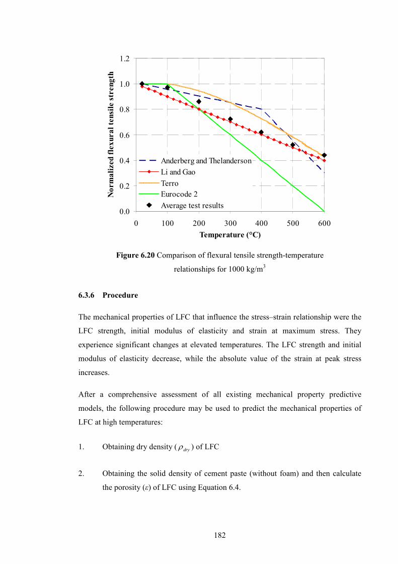
182
0.0
0.2
0.4
0.6
0.8
1.0
1.2
0 100 200 300 400 500 600
Temperature (°C)
�o
rm
ali
zed
fle
xu
ra
l te
nsi
le s
tren
gth
Anderberg and ThelandersonLi and Gao
Terro Eurocode 2
Average test results
Figure 6.20 Comparison of flexural tensile strength-temperature
relationships for 1000 kg/m3
6.3.6 Procedure
The mechanical properties of LFC that influence the stress–strain relationship were the
LFC strength, initial modulus of elasticity and strain at maximum stress. They
experience significant changes at elevated temperatures. The LFC strength and initial
modulus of elasticity decrease, while the absolute value of the strain at peak stress
increases.
After a comprehensive assessment of all existing mechanical property predictive
models, the following procedure may be used to predict the mechanical properties of
LFC at high temperatures:
1. Obtaining dry density ( dryρ ) of LFC
2. Obtaining the solid density of cement paste (without foam) and then calculate
the porosity (ε) of LFC using Equation 6.4.

183
3. Calculating the ambient temperature compressive strength ( cf ) and modulus of
elasticity ( cE ) of LFC using Equation 6.2 and Equation 6.3 respectively. Values
of 39.2 N/mm2 and n=2.4 for the compressive strength and 32.9N/mm2 and
n=2.8 for the compressive modulus of elasticity should be used.
4. Eurocode 2 model (Equation 6.6) to calculate LFC compressive strength ( cTf )
at high temperatures was used.
5. Calculating LFC modulus of elasticity ( cTE ) at high temperatures using the Li
and Purkiss model (Equation 6.11).
6. Multiplying the elastic strain at peak stress by 1.78 to give the strain at peak
stress.
7. Using the Eurocode 2 equation (Equation 6.19) to calculate and plot the stress-
strain relationship of LFC.
8. Calculating the tensile strength of LFC using the equation (Equation 6.21) of Li
and Guo (1993).
6.4 PROPOSED PROCEDURE USI�G COMBI�ED MODEL
The above procedure has been implemented for all the tests carried out in this study.
This section presents detailed comparison between the predicted stress-strain
relationships using the above procedure and the experimental results. Figures 6.21(a-e)
showed the comparison between the predicted stress-strain relationships using the
proposed procedure and the average experimental results of different densities (650
kg/m3 to 1400 kg/m3) at different temperatures. Shown in these figures were also
predicted stress-strain relationships if the measured ambient temperature strength and
modulus of elasticity values were used instead of using the proposed strength-porosity
(Equation 6.2) and modulus of elasticity-porosity (Equation 6.3) relationships. Overall
the agreement was good, demonstrating the feasibility of using the proposed procedure
to predict the mechanical properties of LFC of different densities at different
temperatures by only knowing one single value of dry density ( dryρ ) of LFC. However,
there was some inaccuracy in the stress-strain relationships using the proposed
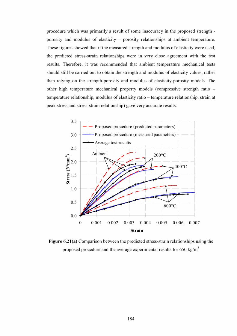
184
procedure which was primarily a result of some inaccuracy in the proposed strength -
porosity and modulus of elasticity – porosity relationships at ambient temperature.
These figures showed that if the measured strength and modulus of elasticity were used,
the predicted stress-strain relationships were in very close agreement with the test
results. Therefore, it was recommended that ambient temperature mechanical tests
should still be carried out to obtain the strength and modulus of elasticity values, rather
than relying on the strength-porosity and modulus of elasticity-porosity models. The
other high temperature mechanical property models (compressive strength ratio –
temperature relationship, modulus of elasticity ratio – temperature relationship, strain at
peak stress and stress-strain relationship) gave very accurate results.
0.0
0.5
1.0
1.5
2.0
2.5
3.0
3.5
0 0.001 0.002 0.003 0.004 0.005 0.006 0.007
Strain
Str
ess
(�
/mm
2)
Proposed procedure (predicted parameters)
Proposed procedure (measured parameters)
Average test results
400°C
200°CAmbient
600°C
Figure 6.21(a) Comparison between the predicted stress-strain relationships using the
proposed procedure and the average experimental results for 650 kg/m3

185
0.0
1.0
2.0
3.0
4.0
5.0
6.0
0 0.001 0.002 0.003 0.004 0.005 0.006
Strain
Str
ess
(�
/mm
2)
Proposed procedure (predicted parameters)
Proposed procedure (measured parameters)
Average test results
400°C
200°CAmbient
600°C
Figure 6.21(b) Comparison between the predicted stress-strain relationships using the
proposed procedure and the average experimental results for 800 kg/m3
0.0
2.0
4.0
6.0
8.0
10.0
0 0.001 0.002 0.003 0.004 0.005 0.006
Strain
Str
ess
(�
/mm
2)
Proposed procedure (predicted parameters)
Proposed procedure (measured parameters)
Average test results
400°C
200°CAmbient
600°C
Figure 6.21(c) Comparison between the predicted stress-strain relationships using the
proposed procedure and the average experimental results for 1000 kg/m3
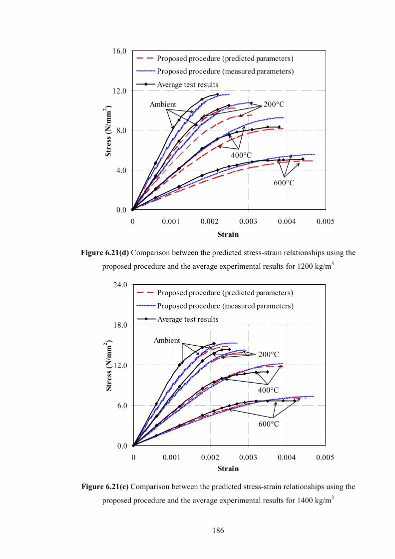
186
0.0
4.0
8.0
12.0
16.0
0 0.001 0.002 0.003 0.004 0.005
Strain
Str
ess
(�
/mm
2)
Proposed procedure (predicted parameters)
Proposed procedure (measured parameters)
Average test results
400°C
200°CAmbient
600°C
`
Figure 6.21(d) Comparison between the predicted stress-strain relationships using the
proposed procedure and the average experimental results for 1200 kg/m3
0.0
6.0
12.0
18.0
24.0
0 0.001 0.002 0.003 0.004 0.005
Strain
Str
ess
(�
/mm
2)
Proposed procedure (predicted parameters)
Proposed procedure (measured parameters)
Average test results
400°C
200°C
Ambient
600°C
Figure 6.21(e) Comparison between the predicted stress-strain relationships using the
proposed procedure and the average experimental results for 1400 kg/m3

187
6.5 CO�CLUSIO�S
This chapter has presented a number of predictive models for mechanical properties of
LFC exposed to elevated temperatures. The experimental results were compared with
predictive models based on normal weight concrete. Since the mechanical properties of
LFC come from Ordinary Portland Cement, thus the change in mechanical properties of
LFC may be predicted using the mechanical property models for normal weight
concrete. The following conclusions may be drawn:
(1) The Balshin equation (Equation 6.1) may be used to calculate both the ambient
temperature compressive strength and compressive modulus of elasticity, as a
function of porosity of LFC. Nevertheless, for improved accuracy, ambient
temperature mechanical property tests were still recommended.
(2) For compressive strength at elevated temperatures, the well accepted Eurocode
2 (2004) model was applicable.
(3) For compressive modulus of elasticity at elevated temperatures, the Li and
Purkiss (2005) model may be used.
(4) For LFC, the total strain at peak stress is approximately 1.78 times the elastic
strain at peak stress.
(5) The Eurocode 2 (2004) equation may be used to obtain the compressive stress-
strain relationship of LFC.
(6) The model of Li and Gao (1993) gave good prediction of the flexural tensile
strength of LFC at elevated temperatures.

188
CCHHAAPPTTEERR 77
SSTTRRUUCCTTUURRAALL PPEERRFFOORRMMAA��CCEE OOFF OO��EE LLFFCC BBAASSEEDD
CCOOMMPPOOSSIITTEE WWAALLLLII��GG SSYYSSTTEEMM
7.1 I�TRODUCTIO�
LFC has very low thermal conductivity, making it a suitable material for building use
as insulating or fire resisting material due to its porous internal structure. LFC can also
be made to have a reliable amount of compressive resistance, making it possible to use
LFC as load-bearing material. However, the experimental results on compressive
properties of LFC presented in Chapter 5 indicated that LFC suffered from brittle
failure. Therefore, a suitable method of using LFC in load-bearing construction would
be to use it in composite action with steel, which has high ductility. This particular
chapter explores the use of LFC in composite action with steel sheeting in lightweight
composite walling construction. Should LFC be cast in-situ, the thin steel sheeting can
be used as formwork during construction. Because of the low density of LFC, the
pressure on the steel sheeting during construction would be much lower than using
normal weight concrete, allowing thin steel sheeting to be used. Before such a system
can be used in practice, it is necessary to carry out fundamental research to thoroughly
investigate its behaviour.
This chapter presents the results of an experimental and analytical investigation into the
structural behaviour of a composite panel system consisting of two outer skins of
profiled thin-walled steel plates with lightweight foamed concrete (LFC) core under
axial compression. A total of 12 tests were carried out, composed of two duplicates of 6
variants which were distinguished by two steel sheeting thicknesses (0.4mm and
0.8mm) and three edge conditions of the sheeting. The density of LFC core was 1000
kg/m3. Experimental results include failure modes, maximum loads and load-vertical

189
strain responses. In analysis, full bond between the steel sheets and the concrete core
was assumed and the LFC was considered effective in restraining inward buckling of
the steel sheets. Using the effective width method for the steel sheets, the load carrying
capacities of the test specimens were calculated and compared with the experimental
results.
7.2 EXPERIME�TS
The experiments were designed to provide information on the load deformation
response and failure modes of the specimens. The objective of the experiments was to
enable development of a calculation method.
7.2.1 Geometrical descriptions of specimen
The dimensions of the test specimens were 400mm high by 400mm wide by 100mm
thick. The short height of the specimens would mean that failure of the specimens
would be governed by cross-sectional capacity. A total of 12 prototype specimens were
tested under axial compression. These 12 specimens consisted of two duplicates of 6
types, being two steel thicknesses (0.4mm and 0.8mm) in combination with three edge
conditions of the steel sheeting. Figure 7.1 showed details of the prototype specimen.
The profiled steel sheeting was made in-house from plain sheeting of 0.4mm or 0.8mm
thickness by fly press. The two profiled steel facings were connected using 6 x 10mm
bolts and nuts.
Refer to Figure 7.2, the steel sheeting could have one of the three edge conditions: (a)
the steel sheets do not cover the LFC panel thickness (referred to as no stopping edge),
(b) the steel sheets cover the LFC panel thickness but were not joined (referred to as
with stopping edges), (c) the steel sheets cover the LFC panel thickness and are joined
by welding (referred to as welded stopping edge). These three steel sheeting edge
conditions were investigated to assess the influence of the steel sheeting in restraining
the LFC to improve its ductility.

190
Figure 7.1 Details of prototype composite walling
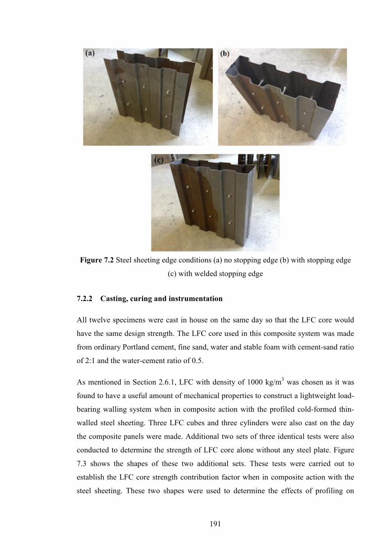
191
Figure 7.2 Steel sheeting edge conditions (a) no stopping edge (b) with stopping edge
(c) with welded stopping edge
7.2.2 Casting, curing and instrumentation
All twelve specimens were cast in house on the same day so that the LFC core would
have the same design strength. The LFC core used in this composite system was made
from ordinary Portland cement, fine sand, water and stable foam with cement-sand ratio
of 2:1 and the water-cement ratio of 0.5.
As mentioned in Section 2.6.1, LFC with density of 1000 kg/m3 was chosen as it was
found to have a useful amount of mechanical properties to construct a lightweight load-
bearing walling system when in composite action with the profiled cold-formed thin-
walled steel sheeting. Three LFC cubes and three cylinders were also cast on the day
the composite panels were made. Additional two sets of three identical tests were also
conducted to determine the strength of LFC core alone without any steel plate. Figure
7.3 shows the shapes of these two additional sets. These tests were carried out to
establish the LFC core strength contribution factor when in composite action with the
steel sheeting. These two shapes were used to determine the effects of profiling on

192
compressive strength of the core, as observed by Wright (1998). LFC was poured
vertically similar to the direction of loading and the test samples were naturally cured in
the indoor climate of the concrete lab. The composite panel was tested at 28 days after
casting.
(a) rectangular LFC panel (b) profiled LFC panel
Figure 7.3 Dimensions of the two additional LFC core samples
A number of strain gauges were placed on the specimens and Figure 7.4 showed their
locations on a sample. In all cases, the strain gauges were at mid-height (h/2) of the
specimen.
Figure 7.4 Strain gauge arrangements

193
7.2.3 Test set-up
The specimens were loaded in axial compression and the test was carried out in a
universal compression testing machine with a maximum capacity of 2,500 kN after 28
days of casting (Figure7.5). The tests were displacement controlled. The top and bottom
of the specimens were ground flat prior to testing so as to ensure equal load
distribution. In addition to the strain gauges on the sample, the displacement of the
loading platen was also recorded to measure axial deformation of the specimen.
Observations were made on general behaviour including cracking of concrete, buckling
of sheeting and failure mode.
Figure 7.5 Axial compression test set-up
7.2.4 Material properties
Three concrete cubes and 3 cylinders were cast and tested on the same days as the
composite walling specimens. The cube tests after 28 days gave an average strength of
5.9 N/mm2 and the cylinder tests provided an average strength of 5.1 N/mm2. The test
results were given in Table 7.1 and they were quite consistent. Table 7.1 also gave the
results of the additional tests on the LFC panels. Data from the steel sheeting supplier
gave yield strength of 280 N/mm2 and a modulus of elasticity of 200,000 N/mm2.
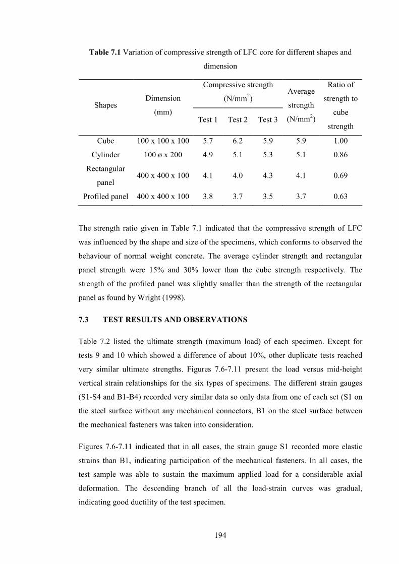
194
Table 7.1 Variation of compressive strength of LFC core for different shapes and
dimension
Compressive strength
(N/mm2) Shapes
Dimension
(mm) Test 1 Test 2 Test 3
Average
strength
(N/mm2)
Ratio of
strength to
cube
strength
Cube 100 x 100 x 100 5.7 6.2 5.9 5.9 1.00
Cylinder 100 ø x 200 4.9 5.1 5.3 5.1 0.86
Rectangular
panel 400 x 400 x 100 4.1 4.0 4.3 4.1 0.69
Profiled panel 400 x 400 x 100 3.8 3.7 3.5 3.7 0.63
The strength ratio given in Table 7.1 indicated that the compressive strength of LFC
was influenced by the shape and size of the specimens, which conforms to observed the
behaviour of normal weight concrete. The average cylinder strength and rectangular
panel strength were 15% and 30% lower than the cube strength respectively. The
strength of the profiled panel was slightly smaller than the strength of the rectangular
panel as found by Wright (1998).
7.3 TEST RESULTS A�D OBSERVATIO�S
Table 7.2 listed the ultimate strength (maximum load) of each specimen. Except for
tests 9 and 10 which showed a difference of about 10%, other duplicate tests reached
very similar ultimate strengths. Figures 7.6-7.11 present the load versus mid-height
vertical strain relationships for the six types of specimens. The different strain gauges
(S1-S4 and B1-B4) recorded very similar data so only data from one of each set (S1 on
the steel surface without any mechanical connectors, B1 on the steel surface between
the mechanical fasteners was taken into consideration.
Figures 7.6-7.11 indicated that in all cases, the strain gauge S1 recorded more elastic
strains than B1, indicating participation of the mechanical fasteners. In all cases, the
test sample was able to sustain the maximum applied load for a considerable axial
deformation. The descending branch of all the load-strain curves was gradual,
indicating good ductility of the test specimen.

195
Table 7.2 Summary of test results of composite walling under compression
Test no. Reference * Steel thickness (mm) Ultimate strength (kN)
0 concrete alone - 125
1 NSE1 161
2 NSE2 0.4
169
3 NSE3 240
4 NSE4 0.8
247
5 WSE1 175
6 WSE2 0.4
187
7 WSE3 263
8 WSE4 0.8
272
9 WE1 189
10 WE2 0.4
207
11 WE3 285
12 WE4 0.8
302
* >SE = no stopping edge; WSE = with stopping edge; WE = welded edge
Table 7.2 showed that the ultimate strength of the specimens with stopping edge was
about 10% higher than those without any stopping edge for both steel thicknesses.
Panels with welded steel edges sustained on average 17% more load than those without
stopping edge. In Section 7.4, it will be shown that these increases in strength can be
attributed to the increase in effective width of the steel sheeting.
Figure 7.12 compares the load versus mid-height strain (point B1) relationships of the
two steel sheeting thicknesses and three edge conditions. As expected, the ultimate load
and axial stiffness of the composite panel increases with increasing steel thickness and
improved edge condition.
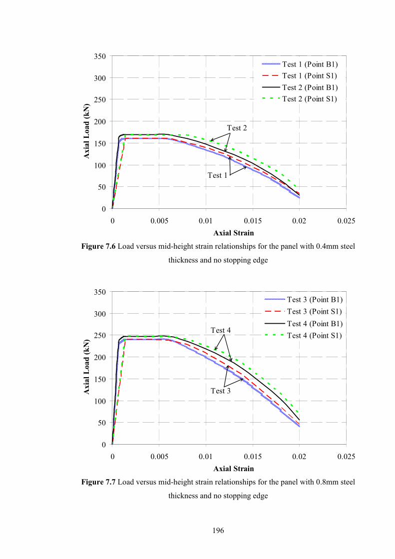
196
0
50
100
150
200
250
300
350
0 0.005 0.01 0.015 0.02 0.025
Axial Strain
Ax
ial
Loa
d (
k�
)
Test 1 (Point B1)
Test 1 (Point S1)
Test 2 (Point B1)
Test 2 (Point S1)
Test 1
Test 2
Figure 7.6 Load versus mid-height strain relationships for the panel with 0.4mm steel
thickness and no stopping edge
0
50
100
150
200
250
300
350
0 0.005 0.01 0.015 0.02 0.025
Axial Strain
Ax
ial
Loa
d (
k�
)
Test 3 (Point B1)
Test 3 (Point S1)
Test 4 (Point B1)
Test 4 (Point S1)
Test 3
Test 4
Figure 7.7 Load versus mid-height strain relationships for the panel with 0.8mm steel
thickness and no stopping edge

197
0
50
100
150
200
250
300
350
0.000 0.005 0.010 0.015 0.020
Axial Strain
Ax
ial
Loa
d (
k�
)
Test 5 (Point B1)
Test 5 (Point S1)
Test 6 (Point B1)
Test 6 (Point S1)
Test 5
Test 6
Figure 7.8 Load versus mid-height strain relationships for the panel with 0.4mm steel
thickness and with stopping edge
0
50
100
150
200
250
300
350
0.000 0.005 0.010 0.015 0.020
Axial Strain
Ax
ial
Loa
d (
k�
)
Test 7 (Point B1)
Test 7 (Point S1)
Test 8 (Point B1)
Test 8 (Point S1)
Test 7
Test 8
Figure 7.9 Load versus mid-height strain relationships for the panel with 0.8mm steel
thickness and with stopping edge

198
0
50
100
150
200
250
300
350
0 0.003 0.006 0.009 0.012 0.015
Axial Strain
Ax
ial
Loa
d (
k�
)
Test 9 (Point B1)
Test 9 (Point S1)
Test 10 (Point B1)
Test 10 (Point S1)
Test 9
Test 10
Figure 7.10 Load versus mid-height strain relationships for the panel with 0.4mm steel
thickness and with welded edge
0
50
100
150
200
250
300
350
0 0.003 0.006 0.009 0.012 0.015Axial Strain
Ax
ial
Loa
d (
k�
)
Test 11 (Point B1)
Test 11 (Point S1)
Test 12 (Point B1)
Test 12 (Point S1)
Test 11
Test 12
Figure 7.11 Load versus mid-height strain relationships for the panel with 0.8mm steel
thickness and with welded edge

199
0
50
100
150
200
250
300
350
0 0.005 0.01 0.015 0.02 0.025 0.03Axial Strain
Axia
l L
oa
d (
k�
)
Test 1 - 0.4mm (no stopping edge)
Test 3 - 0.8mm (no stopping edge)
Test 5 - 0.4mm (with stopping edge)
Test 7 - 0.8mm (with stopping edge)
Test 9 - 0.4mm (welded edge)
Test 11 - 0.8mm (welded edge)
Test 1
Test 11
Test 5
Test 9Test 3
Test 7
`
Figure 7.12 Comparison of load versus mid-height strain (point B1) relationships of the
two steel sheeting thicknesses and three edge conditions and also with profiled panels
without steel sheeting.
Figures 7.13 shows a failed sample for all three edge conditions; (a) without stopping
edge, (b) with stopping edge and (c) with welded edge. The steel sheeting experienced
local buckling before failure, but the LFC core of 1000 kg/m3 density was capable of
preventing the panel from inward buckling. In all cases, failure of the panel was
initiated by local buckling of the steel sheeting, followed by crushing of the LFC core.
Although the steel sheeting provided some ductility to the panel, the welded steel edges
were not able to provide much confinement effect to the LFC panel. It should be
pointed out that the line of bolts should not be a problem. The steel sheeting buckled
and the bolts stopped that. There was no separation of the steel sheeting from the LFC
core until near failure, indicating that the mechanical fasteners were able to hold the
steel sheeting and the LFC core together to enable them to resist the applied load in
composite action. Clearly, if composite walling system using LFC is to be used in real
projects, bond between the profiled steel sheeting and the LFC infill should be

200
considered. However, it is expected that because LFC would be less demanding owing
to its lower strength than normal weight concrete, the steel sheeting used in composite
walling systems using normal weight concrete would still be suitable.
(a) failure mode of panel without stopping edge with outward buckling of steel
(b) failure mode of specimen with stopping edge
(c) failure mode of specimen with welded edge
Figure 7.13 Failure modes for composite panel without stopping edge

201
7.4 A�ALYTICAL RESULTS
As previously described, the panels can be considered to be in composite action and the
LFC core was able to prevent the steel sheeting from inward local buckling. Therefore,
the test specimens will be analysed as a conventional composite walling system.
Since the test panels were short (height to thickness ratio=4), no global buckling was
observed and the panel strength reached the cross-sectional resistance. Also
experimental observation indicates that there was little evidence (e.g. bulging of the
steel sheeting) of any confinement effect on the LFC core provided by the steel
sheeting. Therefore the ultimate resistance of the panel, >u may be calculated from:
csu >>> += ….(7.1)
Where >s is the resistance of the steel sheeting and >c the resistance of the LFC core.
The following sections will discuss how >s and >c may be obtained.
7.4.1 Steel sheeting resistance
7.4.1.1 Critical local buckling stress
The local buckling stress of the steel plate in concrete-filled steel section was
influenced by the width to thickness ratio, boundary condition, initial geometric
imperfection and residual stresses induced by welding or cold-formed process (Liang
and Uy, 2000). For ideal steel plates, the critical elastic buckling stress can be
determined by the following equation (Bulson, 1970):
22
2
)/)(1(12 p
scr
tbv
Ek
−=
πσ ….(7.2)
where σcr is the local buckling stress, k is the elastic buckling coefficient, which
accounts for the effect of the plate aspect ratio and boundary condition on the critical
buckling stress, Es is the modulus of elasticity of the steel, ν is the Poisson’s ratio, b is
the width of the plate and tp is the thickness of the plate.

202
7.4.1.2 Plate buckling coefficient
The plate buckling coefficient of the steel section depends on the boundary condition.
Therefore, the buckling coefficient was a function of the boundary condition along the
longitudinal edges and the type of loading. The k values for various common boundary
conditions and loading cases are given by a few authors (Gerald and Becker, 1957),
(Uy and Bradford, 1996). Gerard and Becker (1957) summarized the buckling
coefficient, k as a function of plate boundary condition and aspect ratio (a/b). Gerard
and Becker’s results are based on steel plates in contact with rigid medium. Uy and
Bradford (1996) recently proposed a slightly different set of plate buckling coefficients
for steel plates in contact with elastic medium, which would be more suitable to the
current problem. For the current research which had uniform distribution of
compressive stress, the buckling coefficients were compared in Table 7.3.
Table 7.3 Buckling coefficient of steel plates under compression
Buckling coefficient, k Boundary condition
Gerald and Becker (1957) Uy and Bradford (1996)
S-F 0.425 0.8
S-S 4 5.6
* S-F – simply supported-free, S-S – simply supported-simply supported
7.4.1.3 Effective width
For thin-walled structures, the current design method was to use an effective width to
account for local buckling. According to Winter (1947), the effective width (beff) of a
plate of width b can be calculated using the following equation:
−
=
y
cr
y
creff
ffb
b σσ22.01 ….(7.3)
Where beff is the effective width, b is the original width, σcr is the local buckling stress,
and fy is the yield stress. The yield stress fy, multiplied by the effective width gives the
ultimate strength of the plate approximately.

203
Liang and Uy (2000) conducted a theoretical study on the post-local buckling
behaviour of steel plates in steel box columns filled with concrete, by using the finite
element method. They found that the post-local buckling characteristics of steel plates
in concrete filled thin-walled box columns have not been adequately studied
theoretically and there is also lack of an efficient method for evaluating the initial local
buckling loads of steel plates. They examined the effective width methods for the
ultimate strength design of steel plates restrained by concrete and of short concrete-
filled welded box columns in compression and proposed the following two effective
width equations:
3
1
675.0
=
y
creff
fb
b σ for σcr ≤ fy ….(7.4)
3
1
915.0
+=
ycr
creff
fb
b
σσ
for σcr > fy ....(7.5)
The resistance of the steel sheeting can be calculated as:
ypeffs ftb> ⋅⋅= ….(7.6)
7.4.2 Strength of LFC core
A study conducted by Wright (1998) established that there was a reduction in load
carrying capacity in profiled concrete panel when compared to solid panel. He found
that the extreme edges of the profiled panel did not present a solid mass of concrete and
the extra bending stresses (due to any loading eccentricity or material non-uniformity)
must be carried by only that concrete in the ribs of the profile. This reduces the load
carrying capacity of the rib to resist the applied axial load.
Wright (1998) then derived an empirical correction to calculate the reduced concrete
strength for uniform axial compression, where the reduction in concrete strength was
assumed to be directly proportional to the extent of void created by profiling the
compressed edge of the panel. A reduction factor, α, which was applied to the concrete
strength was given as below:

204
c
vf
A
A−= 1α ….(7.7)
where Avf is the area of the profile voids on one face and Ac is the area of concrete. For
the tested samples, the calculated α value is 0.91.
The test results in Table 7.1 appeared to confirm the findings by Wright (1998) where
the compressive strength of the profiled LFC panel was found to be lower than the
concrete strength of the solid panel. Therefore, an experimental correction (α reduction
factor in Equation 7.6) must be included when calculating the resistance of the LFC
core in the composite walling system.
Based on this result, the resistance of the LFC core in the proposed composite walling
system can be determined as follows:
α⋅⋅⋅= cucc fA> 69.0 ….(7.8)
The factor of 0.69 (see Table 7.1) takes into account the reduced strength of LFC in a
panel construction compared to the cube strength of LFC, and it was determined by
divided the average solid panel strength (4.1 N/mm2) by the cube strength (5.9 N/mm2).
With the introduction of α calculated using Equation 7.7 (0.91), Equation 7.8 gives a
final factor of 0.63 which was the same as the experimental result in Table 7.1,
obtained by dividing the LFC strength in the profiled panel by the LFC cube strength.
7.4.3 Load carrying capacity of composite wall panels
Based on the discussion in the last section, the load carrying capacity (>u) of the
composite wall panel in axial compression, taking into consideration the effective width
and concrete strength reduction factor for profiled shape, can be calculated by using the
following equation:
ypeffcucu ftbfA> ⋅⋅+⋅⋅= 63.0 ….(7.9)
Table 7.4 presented the total effective width of steel sheeting for the two different
thicknesses and the three different edge conditions, using the aforementioned two
different methods of calculating the plate buckling coefficient and two methods of
calculating the plate effective width. The total effective width coefficient was obtained
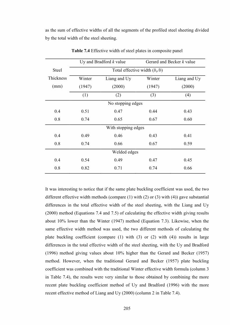
205
as the sum of effective widths of all the segments of the profiled steel sheeting divided
by the total width of the steel sheeting.
Table 7.4 Effective width of steel plates in composite panel
Uy and Bradford k value Gerard and Becker k value
Total effective width (be/b)
Winter
(1947)
Liang and Uy
(2000)
Winter
(1947)
Liang and Uy
(2000)
Steel
Thickness
(mm)
(1) (2) (3) (4)
No stopping edges
0.4 0.51 0.47 0.44 0.43
0.8 0.74 0.65 0.67 0.60
With stopping edges
0.4 0.49 0.46 0.43 0.41
0.8 0.74 0.66 0.67 0.59
Welded edges
0.4 0.54 0.49 0.47 0.45
0.8 0.82 0.71 0.74 0.66
It was interesting to notice that if the same plate buckling coefficient was used, the two
different effective width methods (compare (1) with (2) or (3) with (4)) gave substantial
differences in the total effective width of the steel sheeting, with the Liang and Uy
(2000) method (Equations 7.4 and 7.5) of calculating the effective width giving results
about 10% lower than the Winter (1947) method (Equation 7.3). Likewise, when the
same effective width method was used, the two different methods of calculating the
plate buckling coefficient (compare (1) with (3) or (2) with (4)) results in large
differences in the total effective width of the steel sheeting, with the Uy and Bradford
(1996) method giving values about 10% higher than the Gerard and Becker (1957)
method. However, when the traditional Gerard and Becker (1957) plate buckling
coefficient was combined with the traditional Winter effective width formula (column 3
in Table 7.4), the results were very similar to those obtained by combining the more
recent plate buckling coefficient method of Uy and Bradford (1996) with the more
recent effective method of Liang and Uy (2000) (column 2 in Table 7.4).

206
Table 7.5 compared the calculated and measured wall panel strengths for all the 12 tests
using the different effective widths of Table 7.4. Due to the relatively low contribution
by the steel sheeting to the strength of the panels, all four methods produced similar
panel strengths. A statistical analysis was carried out to verify the homogeneity and the
reliability of the predicted strength over experimental results obtained from the
proposed equation (Equation 7.9). The mean x and standard deviation s, were calculated
for each combination of design method as shown in Table 7.5. Overall, the ratio of
predicted strength-experiment results using all the four methods indicated that the
specimens were relatively homogeneous.
Among these four methods, both the effective widths (2) and (3) in Table 5 gave good
estimation of panel strength. Among these two methods, the method (2) appeared to
give slightly more accurate predictions. The results in Table 7.5 were also presented in
Figures 7.14-7.16. It should be pointed out that the buckling coefficient for plates from
Uy and Bradford (1996) and effective width formulation proposed by Liang and Uy
(2000) respectively were derived for composite column design. From the results in
Table 7.5, these models were also acceptable for design use for composite panel using
LFC.

207
Table 7.5 Comparisons between predicted composite panel strengths and test results
Predicted Strength (kN) Ratio predicted/experiment
Gerard and
Becker k value
Uy and Bradford
k value
Gerard and
Becker k value
Uy and Bradford
k value Ref.
No. Liang
and Uy Winter
Liang
and Uy Winter
Liang
and Uy Winter
Liang
and Uy Winter
NSE1 1.05 1.06 1.08 1.10
NSE2 169 171 174 177
1.00 1.01 1.03 1.05
NSE3 1.02 1.08 1.07 1.14
NSE4 245 259 256 273
0.99 1.05 1.04 1.11
WSE1 1.01 1.02 1.04 1.07
WSE2 177 179 182 187
0.95 0.96 0.98 1.00
WSE3 1.03 1.09 1.09 1.16
WSE4 270 288 286 306
0.99 1.06 1.05 1.12
WE1 0.96 0.97 0.99 1.02
WE2 182 184 187 192
0.88 0.89 0.90 0.93
WE3 1.01 1.08 1.05 1.14
WE4 287 307 300 325
0.95 1.02 0.99 1.07
Mean, x 0.9867 1.0242 1.0258 1.0758
Standard deviation, s 0.0458 0.0596 0.0532 0.0674

208
0
100
200
300
400
500
0 0.2 0.4 0.6 0.8 1 1.2Profile thickness (mm)
Ax
ial
loa
d (
k�
)
Winter effective width with Uy & Bradford k value
Liang & Uy effective width with Uy & Bradford k valueWinter effective width with Gerrard & Becker k value
Liang & Uy effective width with Gerrard & Becker k valueTest results
Figure 7.14 Comparisons between predicted strengths and test results for composite
panel with no stopping edge
0
100
200
300
400
500
0 0.2 0.4 0.6 0.8 1 1.2Profile thickness (mm)
Ax
ial
loa
d (
k�
)
Winter effective width with Uy & Bradford k value
Liang & Uy effective width with Uy & Bradford k value
Winter effective width with Gerrard & Becker k value
Liang & Uy effective width with Gerrard & Becker k value
Test results
Figure 7.15 Comparisons between predicted strengths and test results for composite
panel with stopping edge

209
0
100
200
300
400
500
0 0.2 0.4 0.6 0.8 1 1.2Profile thickness (mm)
Ax
ial
loa
d (
k�
)
Winter effective width with Uy & Bradford k value
Liang & Uy effective width with Uy & Bradford k value
Winter effective width with Gerrard & Becker k value
Liang & Uy effective width with Gerrard & Becker k value
Test results
Figure 7.16 Comparisons between predicted strengths and test results for composite
panel with welded edge
7.5 CO�CLUSIO�S
This chapter has described two series of tests on a new composite wall panel system
consisting of two outer skins of profiled thin-walled steel sheeting with lightweight
foamed concrete (LFC) core under axial compression, for steel sheeting thicknesses of
0.4mm and 0.8mm respectively. Each series of tests had three edge conditions for the
sheeting. These tests provided information on the behaviour and failure mode of these
panels. An analytical model has been developed to calculate the maximum load-bearing
capacity of this type of wall system. It was found from the experimental investigation
that the failure of the panel system was initiated by outward local buckling of the steel
sheeting which was followed by concrete crushing of the LFC core and the LFC core of
1000 kg/m3 density was sufficient to prevent the steel sheeting from inward buckling.
All the specimens showed good ductility, giving gradual reduction in load carrying
capacity at increasing deformation. In contrast, without using steel sheeting, the core
LFC panels experienced brittle failure after reaching the peak load. The increase in load
carrying capacities of the panels with stopping edge and welded edge can be attributed

210
to the increased effective width of the steel sheeting. The load carrying capacities of
panels with stopping edge and with welded edge were about 10% and 17% higher than
those without any stopping edge for both steel sheeting thicknesses.
The proposed panel strength calculation model which takes into consideration the effect
of profiling on concrete strength according to Wright was able to predict the axial
capacity of the proposed panel very well. For calculating the steel sheeting effective
width, the combination of Uy and Bradford plate local buckling coefficients with the
Liang and Uy effective width formulation appeared to give the best agreement with the
experimental results. Nevertheless, the traditional effective width method proposed by
Winter in conjunction with the traditional plate local buckling coefficients of Gerard
and Becker also gave close results compared to the experiments.

211
CCHHAAPPTTEERR 88
II��DDIICCAATTIIVVEE SSTTUUDDYY OO�� FFIIRREE RREESSIISSTTAA��CCEE AA��DD
SSTTRRUUCCTTUURRAALL PPEERRFFOORRMMAA��CCEE OOFF LLFFCC BBAASSEEDD SSYYSSTTEEMM
8.1 I�TRODUCTIO�
This research so far has primarily concentrated on developing and validating thermal
property models for LFC, characterizes its mechanical properties at high temperatures
and concentrated on experimental and analytical studies of the structural behaviour and
ultimate load carrying capacity of a composite walling system under axial compression.
From the experimental verification, as expected the mechanical properties of LFC were
reasonably low when compared to normal weight concrete. Nonetheless there was a
potential of using LFC as fire resistant partition or as load-bearing walls in low-rise
residential construction. In order to demonstrate the feasibility of this proposal, this
chapter presents a preliminary feasibility study on its fire resistance and structural
performance of LFC based system. The objectives of this feasibility study were:
• Investigating the fire resistance performance of LFC panels of different
densities (650, 800, 1000, 1200 and 1400 kg/m3) when exposed to fire on one
side for different fire resistance ratings based on insulation requirement.
• Examining whether the composite walling system had sufficient load carrying
capacity, based on compression resistance at ambient temperature.

212
8.2 ASSESSME�T OF FIRE RESISTA�CE PERFORMA�CE I� THE
CO�TEXT OF FIRE REQUIREME�TS STA�DARD
When designing a building, a very significant consideration is how it will behave in fire
and ensure the elements of structure will not collapse but remain standing or hold back
the fire for a prescribed time. The building regulation stipulates the rules and the degree
of fire resistance of the elements of structure. For example, BS 476 (1987) dictates the
appropriate fire tests for these elements of structure and materials and grades the level
of fire resistance.
The author planned to develop and utilize this LFC panel system in Malaysia therefore
discussion in this section will include the fire requirements stipulated in the Malaysia
standard as well. All building constructions in Malaysia have to abide by the fire
requirements specified in Part VII of the UBBL (1997). These requirements include the
restrictions on spread of flame and fire resistance of structural members. The Ninth
Schedule of the UBBL gives the minimum requirements for fire resistance (in hours)
for single-storey (Part II) and multi-storey (Part I) buildings of various types. It also
gave the notional fire rating values of various common types of construction. Similar
fire requirements standard can also be found in other building by-laws and codes. The
minimum statutory fire rating requirements for elements of structure in Malaysia and
England are summarised in Table 8.1, for brevity and easy comparison.
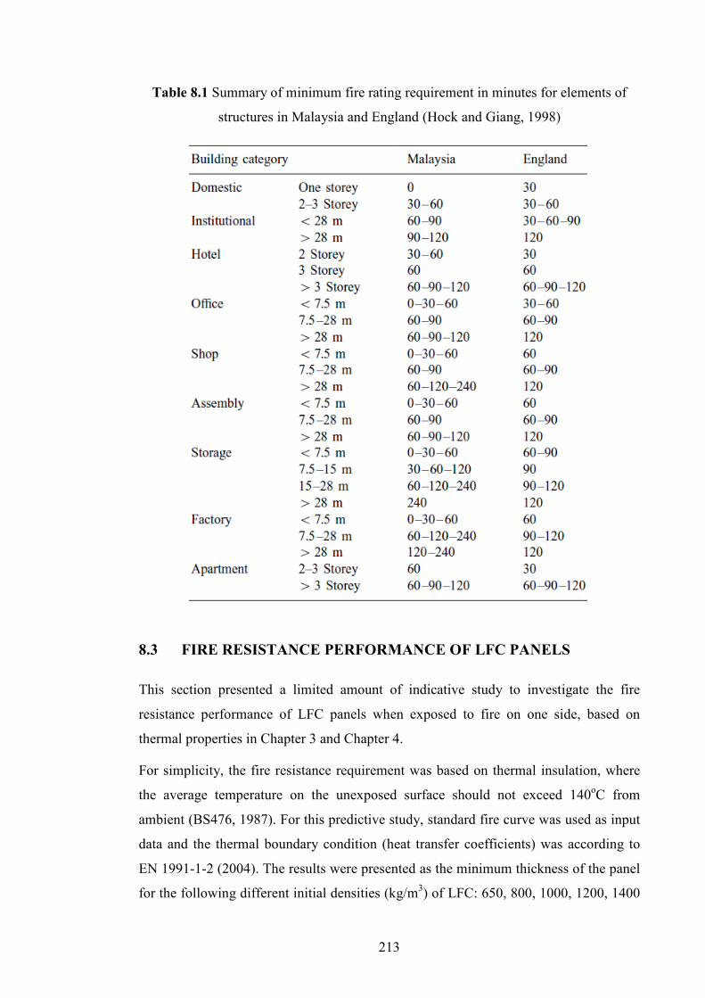
213
Table 8.1 Summary of minimum fire rating requirement in minutes for elements of
structures in Malaysia and England (Hock and Giang, 1998)
8.3 FIRE RESISTA�CE PERFORMA�CE OF LFC PA�ELS
This section presented a limited amount of indicative study to investigate the fire
resistance performance of LFC panels when exposed to fire on one side, based on
thermal properties in Chapter 3 and Chapter 4.
For simplicity, the fire resistance requirement was based on thermal insulation, where
the average temperature on the unexposed surface should not exceed 140oC from
ambient (BS476, 1987). For this predictive study, standard fire curve was used as input
data and the thermal boundary condition (heat transfer coefficients) was according to
EN 1991-1-2 (2004). The results were presented as the minimum thickness of the panel
for the following different initial densities (kg/m3) of LFC: 650, 800, 1000, 1200, 1400
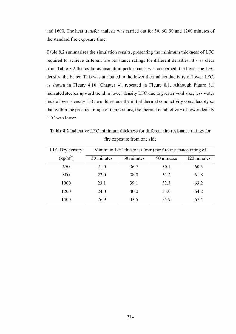
214
and 1600. The heat transfer analysis was carried out for 30, 60, 90 and 1200 minutes of
the standard fire exposure time.
Table 8.2 summarises the simulation results, presenting the minimum thickness of LFC
required to achieve different fire resistance ratings for different densities. It was clear
from Table 8.2 that as far as insulation performance was concerned, the lower the LFC
density, the better. This was attributed to the lower thermal conductivity of lower LFC,
as shown in Figure 4.10 (Chapter 4), repeated in Figure 8.1. Although Figure 8.1
indicated steeper upward trend in lower density LFC due to greater void size, less water
inside lower density LFC would reduce the initial thermal conductivity considerably so
that within the practical range of temperature, the thermal conductivity of lower density
LFC was lower.
Table 8.2 Indicative LFC minimum thickness for different fire resistance ratings for
fire exposure from one side
Minimum LFC thickness (mm) for fire resistance rating of LFC Dry density
(kg/m3) 30 minutes 60 minutes 90 minutes 120 minutes
650 21.0 36.7 50.1 60.5
800 22.0 38.0 51.2 61.8
1000 23.1 39.1 52.3 63.2
1200 24.0 40.0 53.0 64.2
1400 26.9 43.5 55.9 67.4

215
0.0
0.1
0.2
0.3
0.4
0.5
0 100 200 300 400 500 600 700 800 900 1000
Temperature (°C)
Th
erm
al
Co
nd
uct
ivit
y (
W/m
°C).
650 kg/m3
800 kg/m3
1000 kg/m3
1200 kg/m3
1400 kg/m3
Figure 8.1 Thermal conductivity-temperature curves for all the densities used in
this parametric study
The results in Table 8.2 indicated that although increasing LFC density would increase
its specific heat, thus allowing more heat to be absorbed in LFC, as far as the
unexposed surface temperature is concerned, which was used to assess insulation fire
performance, thermal conductivity plays a more important role so that using higher
density LFC had no advantage. The minimum thickness values in Table 8.2 were not
particularly onerous. In fact, a single layer of 650 kg/m3 density LFC of about 21 mm
would achieve 30 minutes of standard fire resistance rating, more or less similar to
gypsum plasterboard. This value is encouraging for application of LFC in building
construction as fire resistant partitions.
From the indicative study results on LFC panels shown in Table 8.2, it can be
concluded that if LFC panel of 100mm thickness of any density (650 to 1400 kg/m3)
was to be used in construction, it was able to meet the various fire rating requirements
stipulated by the UBBL (1997) for thermal insulation. For domestic construction, a fire
resistance rating of 30 minutes can be easily met by LFC panels.

216
8.4 FEASIBILITY OF USI�G LFC BASED COMPOSITE WALLI�G
SYSTEM
The potential market for this composite walling system is low-rise residential
construction. The practicability of this system was examined by analysing the
investigation to verify whether the composite walling system has sufficient load
carrying capacity. It was proposed to construct the interior load-bearing walls by using
100mm thick composite walls with 0.4mm steel sheeting, as tested in this research
(presented in Chapter 7). Figure 8.2 showed the elevation section of a four-storey
residential building and the floor span is 5m. Table 8.3 summarizes the applied loads on
the interior walls (panels 1-4) supporting different floors.
Figure 8.2 Arrangement of LFC composite wall panels for a four-storey residential
building section.

217
Table 8.3 Design of prototype composite panel
Description Unit Value
Slab thickness mm 150
Dead load (partitions and finishes) kN/m2 1.5
Imposed loads (floor) kN/m2 2.5
Self weight of slab (with normal weight
concrete) kN/m =0.15*24*5=18.0
Partition and finishes kN/m =5*1.5=7.5
Characteristic dead load, Gk kN/m =18+7.5=25.5
Characteristic imposed load, Qk kN/m =5*2.5=12.5
Design load, F kN/m =(1.4*25.5)+(1.6*12.5)=55.7
Self weight of the panel (100 mm thick wall
of 1000 kg/m3) kN/m 3.2
Load carried by Panel 1 kN/m 55.7
Load carried by Panel 2 kN/m 114.6
Load carried by Panel 3 kN/m 173.5
Load carried by Panel 4 kN/m 232.4
Table 8.4 compared the applied loads (per 0.4m) on the different panels with the
available panel strengths (per 0.4m) based on the experimental results in Table 7.2. It
was expected that the 3m wall panel as proposed in Figure 8.2 will have a lower
strength than the 400mm high test panels due to buckling. This will be further
examined in Section 8.5, based on flexural buckling resistance. However, the results in
Table 8.4 clearly indicated the 100mm thick panel with 0.4mm steel sheeting has
sufficient cross-sectional resistance for four floors.

218
Table 8.4 Assessment of adequacy of 100mm thick wall with 0.4mm thick steel
sheeting.
Wall adequate based on average experimental
results in Table 7.2 (Chapter 7)
Description
Required load carrying
capacity per 0.4m wide
(kN)
no stopping
edge
(165kN)
with stopping
edge
(181kN)
with welded
stopping edge
(198kN)
Panel 1 = 0.4*55.7 = 23 √ √ √
Panel 2 = 0.4*114.6 = 46 √ √ √
Panel 3 = 0.4*173.5 = 70 √ √ √
Panel 4 = 0.4*232.4 = 93 √ √ √
8.5 EFFECT OF SLE�DER�ESS RATIO O� LOAD CARRYI�G
CAPACITY OF COMPOSITE WALLI�G SYSTEM
It was expected that the strength of the proposed composite walling system will
decrease increasing height due to buckling effect.
The flexural buckling resistance of panel under compression may be calculated using
the well known Euler equation (Gere, 2004) given below:
2
2
p
crL
EIP
π= ……(8.1)
where Pcr is the critical buckling load; EI (=EsIs + EcIc) is the flexural rigidity of the
composite cross section with Es and Ec being the Young's modulus of steel and LFC
respectively and Is and Ic being the second moment of area of the steel sheeting and
LFC core respectively about the centre of the composite cross-section. Es = 200,000
N/mm2 and Ec = 3,300 N/mm2. Lp is the length of composite panel.
Figure 8.3 clearly compared the buckling resistance of 400mm wide panels of two
types of construction (with or without stopping edge) for panel heights ranging from
2m to 5m.

219
0
50
100
150
200
250
300
350
1.0 2.0 3.0 4.0 5.0 6.0
Panel length (m)
Cri
tica
l b
uck
lin
g l
oa
d (
k�
)
Without stopping edge
With stopping edge
Figure 8.3 Relationship between critical load and panel height, panel width=400mm
Table 8.5 listed the applied loads (per 0.4m) for the different panels of the indicative
building shown in Figure 8.1 with the calculated buckling strengths (per 0.4m) for
different panel heights. The results showed that if the panel height does not exceed 3m,
which would be sufficient to cover most cases of residential construction, the proposed
panel system would have sufficient load carrying capacity. For heights of 4 and 5m, the
proposed panel construction would not be sufficient for three storeys, but would be
sufficient for one or two storey residential construction. For such heights, the panel
thickness and steel sheeting thickness could be increased to increase the panel load
carrying capacity. It should be pointed out that full composite action is not likely to
take place between the steel sheeting and LFC core. Interaction between the steel
sheeting and the LFC core was generated using mechanical bolts for the samples tested
in this research. Nevertheless these mechanical fasteners that connected the two
profiled steel facings with the concrete core were able to give some degree of
composite action and preventing the steel from peeling off during loading. It is
suggested that future work is necessary to develop a better bonding system for practical
application. The main conclusion was that the LFC based composite walling system
could be designed to resist the applied loads in low-rise residential construction.

220
Table 8.5 Assessment of adequacy of 100mm thick wall with 0.4mm thick steel
sheeting for different panel lengths
Panel length (m) 2.0 3.0 4.0 5.0
Length-width ratio 5.0 7.5 10.0 12.5
Edge condition Required load carrying
capacity per 0.4m wide
Wall adequate based on critical
buckling load calculation
Panel 1 (23kN) √ √ √ √
Panel 2 (46kN) √ √ √ x
Panel 3 (76kN) √ √ x x
No stopping edge
Panel 4 (93kN) √ √ x x
Panel 1 (23kN) √ √ √ √
Panel 2 (46kN) √ √ √ √
Panel 3 (76kN) √ √ x x
With stopping edge
Panel 4 (93kN) √ √ x x
Panel 1 (23kN) √ √ √ √
Panel 2 (46kN) √ √ √ √
Panel 3 (76kN) √ √ x x
Welded edge
Panel 4 (93kN) √ √ x x
8.6 SUMMARY
This short chapter has presented the results of a feasibility study to investigate the
potential of using LFC in lightweight residential construction, considering the
insulation performance for fire resistance and compressive resistance of LFC wall
panels at ambient temperature.
From the fire resistance investigation, it had been concluded that the LFC based panel
system exposed to the standard fire on one side can easily achieve the insulation
performance requirement with a very small thickness, the minimum LFC panel
thickness for the highest density (1400kg/m3) being around 26.9mm, 43.5mm, 55.9mm
and 67.4mm for 30, 60, 90 and 120 minutes of standard fire rating respectively. This
performance was very similar to that provided by gypsum plasterboards. Because of the
dominant role played by thermal conductivity, lighter LFC tends to perform better
because of its low thermal conductivity.

221
From a comparison between squash resistance and Euler buckling load of LFC based
composite walling systems against applied loads on a low-rise residential structure with
typical floor loads and spans, it had been concluded that the LFC based walling system
can be easily designed to achieve four storeys with typical floor heights between 2-5m.
Although there were a number of issues should still be investigated in detail in order to
fine tune the design process, this study has confirmed the applicability of LFC based
panel walling system to lightweight low-rise residential construction.
222
CCHHAAPPTTEERR 99
CCOO��CCLLUUSSIIOO��SS AA��DD RREECCOOMMMMEE��DDAATTIIOO��SS FFOORR
FFUUTTUURREE WWOORRKK
This chapter presented a summary of the main conclusions of this study and gives some
recommendations for future research on LFC.
9.1 SUMMARY A�D CO�CLUSIO�S
Lightweight foamed concrete (LFC) was primarily used as a void filling and insulation
material but it has a number of favourable characteristics such as light weight, good
acoustic and insulation performance, ease in fabrication, environmentally sustainable,
durable and cost effective. This had led LFC to be considered as a possible load-bearing
material for building construction.
An extensive literature review in Chapter 2 had indicated that most of the researches
have focused on LFC ambient temperature properties only and very little information
was available on LFC thermal and mechanical properties at elevated temperatures. Also
there were very few research studies to investigate structural performance and fire
resistance of LFC based systems. Filling these major gaps in knowledge became the
main objectives of this research. The following major tasks were undertaken to achieve
the objectives of this research:
• Small-scale high temperature tests on LFC specimens (Chapter 3).
• Development of analytical models of thermal conductivity and specific heat of
LFC (Chapter 3).
• Validation of thermal properties model and sensitivity study (Chapter 4).
• Mechanical properties tests of LFC at high temperatures (Chapter 5).

223
• Characterization of mechanical properties of LFC exposed to high temperatures
(Chapter 5)
• Predictive equations for mechanical properties of LFC based on existing models
for normal weight concrete (Chapter 6).
• Structural tests on prototype LFC based composite walling system consisting of
two outer skins of profiled thin-walled steel sheeting with lightweight foamed
concrete (LFC) core under axial compression (Chapter 7).
• Development of analytical model to calculate the maximum load-bearing
capacity of this composite walling system (Chapter 7).
• Feasibility study on fire resistance and structural performance of LFC based
system (Chapter 8).
From these research investigations, the following main conclusions may be drawn:
• For the purpose of establishing the thermal conductivity values of LFC at
elevated temperatures, two methods may be considered: direct measurement
using the hot guarded plate (HGP) test method and analytical method based on
porous material. The analytical method has the advantage of providing
fundamental understanding of the material and the thermal conductivity value
can be determined with a minimum input of material property data at high
temperatures. This contrasts with the HGP test method in which separate tests
will be required for different temperatures. The superiority of the analytical
model over the HGP test was that LFC of different densities may be now
considered without relying on extensive tests.
• The development of the analytical method to determine the thermal conductivity
of LFC at high temperatures was based on treating LFC as mix of dried LFC
and water before completion of water evaporation and as mix of dried LFC and
air voids afterwards. The thermal conductivity of dried LFC and average air
void size should be determined in order to employ the analytical model. The
void size may be acquired by taking a microscopic image of the LFC and the
dried thermal conductivity value of LFC can be directly measured using the

224
HGP test or calculated if the LFC ambient temperature thermal conductivity
was available. This chapter has presented detailed guidance on how to perform
these calculations. A comparison between measured thermal conductivity
results using the guarded hot plate test and the predicted thermal conductivity
results using the theoretical model showed very good agreement.
• The specific heat of LFC can be approximated as the sum of a constant base
value for the dried LFC and an additional value to allow for heat required to
evaporate the free water.
• Given that the mechanical properties of LFC come from Ordinary Portland
Cement, it has been confirmed that the reduction in mechanical properties of
LFC can be predicted using the mechanical property models for normal weight
concrete.
• From structural tests on LFC based composite walling system consisting of two
outer skins of profiled thin-walled steel sheeting with LFC core under axial
compression, for steel sheeting thicknesses of 0.4mm and 0.8mm respectively, it
was found that all the specimens demonstrated good ductility, giving gradual
reduction in load carrying capacity at increasing deformation. Failure of the
composite walling was instigated by outward local buckling of the steel sheeting
which was followed by concrete crushing of the LFC core. LFC was able to
provide sufficient support to prevent the steel sheeting from inward buckling.
• Edge detailing of the LFC based composite walling system had some influence
on the ultimate strength of the system. Covering the edges of the panels with
steel sheeting improved the panel strength. Welding the steel sheeting at the
edges (referred to as welded edge) to form a closed tubular construction gave
higher load carrying capacity than without joining them (referred to as with
stopping edges). Compared to LFC panels without the steel sheeting covering
the edges, the load carrying capacities of panels with stopping edge and with
welded edge were about 10% and 17% higher.
• The cross-sectional resistance of the LFC based composite walling system may
be calculated by adding together the resistance of the steel sheeting and the

225
resistance of the profiled LFC core. For the LFC core, profiling results in a
reduction of its strength due to unavoidable small eccentricity reducing the
effectiveness of the LFC at the extremities of the core. The model proposed by
Wright (1998), based on test results for normal weight concrete walling system,
was found applicable to profiled LFC cores. In order to deal with local buckling
of the steel sheeting, the combination of Uy and Bradford (1996) plate local
buckling coefficients with the Liang and Uy (2000) effective width formulation
to work out the steel sheeting effective width appears to provide the best
agreement with the experimental results. Nevertheless, good agreements with
test results were also established when using more traditional approach for the
effective width method proposed by Winter (1947) in conjunction with the plate
local buckling coefficients of Gerard and Becker (1957).
• The indicative study of fire resistance performance of LFC construction under
standard fire exposure from one side has concluded that LFC has outstanding
insulation performance for fire resistance and offers a practicable alternative to
gypsum as the construction material for partition walls. For instant, a single
layer of 650 kg/m3 density LFC of about 21 mm would achieve 30 minutes of
standard fire resistance rating, more or less similar to gypsum plasterboard.
• The results of a feasibility study on structural performance of composite panel
system has confirmed it would be possible to design LFC based composite
walling system to resist typical floor loads in low rise residential construction.
For example, using 100mm LFC core and 0.4mm steel sheeting would give
sufficient load carrying capacity for the construction of 4 storey buildings with
3m storey height.
9.2 RECOMME�DATIO� FOR FUTURE RESEARCH STUDIES
The author believes that this thesis represents the first comprehensive experimental and
analytical study on thermal and mechanical properties of LFC at high temperatures and
structural performance of composite walling system with LFC core. Inevitably, a
number of assumptions have been made and some conclusions had been drawn based
on limited available experimental data. While this study has filled some important gaps
in knowledge related to LFC subject, it had also identified the need to execute more

226
comprehensive further research studies on LFC properties, structural behavior, fire
resistance and other building construction requirements. In particular, this thesis
recommends the following specific studies related to material specification, structural
behaviour and fire resistance:
9.2.1 On material specification and properties
• The present study had concentrated on using a constant cement-sand ratio of 2:1
and water cement ratio of 0.5. Future work is necessary to look into different
cement-sand ratios and water-cement ratios on thermal and mechanical
properties of LFC at elevated temperatures.
• It was established from the literature review that utilization of fly ash as filler in
LFC mix may contribute to better strength and thermal conductivity. Therefore
it would be desirable for future studies to look into this effect.
• Similarly, it may be possible to improve the properties of LFC by using fibre,
which may help reduce the size of the pores without increasing the LFC density.
• The present experimental and numerical studies on thermal and mechanical
properties were limited to two LFC densities. Future studies should place
greater emphasise on different densities as well.
• It would be ideal if the mechanical properties of LFC at elevated temperatures
could be predicted numerically, taking into consideration the mechanical
properties of the solid constituent and the effects of pores.
• The elevated temperature mechanical property tests presented in this study were
under the steady state condition. Transient state tests, although being more
difficult, may become necessary. Also, the tests in this study were conducted to
obtain mechanical properties of unstressed samples at high temperatures. Other
mechanical properties, including the effect of pre-stress, residual properties after
cooling down, thermal strain at high temperatures, should also be investigated.

227
9.2.2 On structural behaviour
• This research had used one type of profiling. It would be interesting to conduct
future studies to look into the effects of different steel profiling.
• The feasibility study in Chapter 8 used either the cross-sectional resistance of
Euler buckling load as the upper limit. Future work is essential to establish
empirical equations to consider their interactions.
• Interaction between the steel sheeting and the LFC core was generated using
mechanical bolts for the samples tested in this research. For practical
application, a better bonding system should be developed.
• The structural tests were conducted on individual samples. Connection between
panels will have important influence on the entire panel behaviour. For practical
construction, such detailing should be carefully investigated. It is recommended
that full scale panel tests should be conducted.
• Bending and combined bending and axial compression behaviour should be
investigated.
• More detailed numerical simulation methods should be developed for both local
buckling effects and global structural behaviour.
9.2.3 On fire resistance
• This study had only carried out an indicative investigation of thermal insulation
performance for fire resistance. Structural load-bearing capacity, one of the
three requirements of fire resistance, should be investigated in the future. In
particular, future investigation should include the effects of non-uniform
temperature distribution in the LFC based system.
• This study had only focused on the structural behaviour of small scale
composite panel system at ambient temperature. In order to demonstrate the
structural performance of LFC based composite panel system in fire, future
studies should concentrate on the effects of elevated temperatures on the
strength of composite system.

228
• Fire integrity, related to preventing fire spread through gaps in construction, is
one of the three requirements of fire resistance. Panel joining detailing will
greatly affect fire integrity. Future research studies should be conducted to
investigate this effect.
• Numerical methods should be developed to carry out combined heat transfer
and structural behaviour analysis under fire condition.
• Performance based fire engineering, in which natural fire condition, as opposed
to the standard fire condition, can be considered. Future research should extend
the current studies to natural fire conditions.
• Methods of assessing and repairing fire damaged LFC construction should be
developed.
229
REFERE�CES
Ai, H., Young, J.F., and Scherer, G. W., “Thermal expansion kinetics: Method to
measure permeability of cementitious materials: II, application to hardened cement
pastes”, J. Am. Ceram. Soc., 84, 385-391 (2001).
Aldridge, D., “Introduction to foamed concrete: What, Why, and How?”, In: Dhir, R.
K., Newlands, M. D., McCarthy, A., Editors; Use of foamed concrete in construction,
London: Thomas Telford, 1-14 (2005).
Aldridge, D., and Ansell, T., “Foamed concrete: production and equipment design,
properties, applications and potential”, In: Proceedings of one day seminar on foamed
concrete: Properties, applications and latest technological developments, Loughborough
University (2001).
Anderberg, Y. and Thelandersson, S. “Stress and deformation characteristics of
concrete at high temperatures: Experimental investigation and material behavior
model", Bulletin 54, Sweden (Lund): Lund Institute of Technology (1976).
Ang, C. N., and Wang, Y. C., “The effect of water movement on specific heat of gypsum
plasterboard in heat transfer analysis under natural fire exposure”, J. Construct. Build.
Mater., 18, 505-515 (2004).
ASTM C 177-97, “Standard test method for steady-state heat flux measurements and
thermal transmission properties by means of the guarded-hot-plate apparatus”,
American Society for Testing and Materials (1997).

230
Balshin, M. Y., “Dependence of mechanical properties of metal powders on porosity
and limiting properties of metal–ceramic materials (in Russian)”, Dokl. Akad. Nauk.
UzSSR, 67, 831-834 (1949).
Bazant, P., and Chern, J. C., “Stress-induced thermal and shrinkage strains in
concrete”, J. Eng. Mech., ASCE, 113, 1493–511 (1987).
Brady, K. C., Watts, G. R. A., and Jones, M. R., “Specification for foamed concrete”,
Prepared for Quality Services, Civil Engineering, Highways Agency (2001).
Brandt, A. M., “Cement-Based Composites: Materials, mechanical properties and
performance”, E & FN Spon, London, 117-118 (1995).
British Cement Association, “Foamed concrete: Composition and properties”, Report
Ref. 46.042, Slough: BCA (1994).
BS 476, “Fire tests on building materials and structures, Part 20: Method for
determination of the fire resistance of elements of construction”, General principles
(1987).
BS EN 197-1, “Cement: Composition, Specifications and conformity criteria for low
heat common cements”, British Standards Institution, London (2000).
BS EN 12620, “Aggregates for Concrete”, British Standards Institution, London
(2002).

231
Bulson, P. S., “The stability of flat plates”, Chatto and Windus, London (1970).
Burns, P. J., and Tien, C.L., “>atural convection in porous media bounded by
concentric spheres and horizontal cylinders”, Int. J. Heat Mass Transfer, 22, 929-939
(1979).
Cabrera, J. G., and Lynsdale, C. J., “A new gas permeameter for measuring the
permeability of mortar and concrete”, Mag. Concr. Res., 40, 177-182 (1988).
Carman, A. P., and Nelson, R. A., “The thermal conductivity and diffusivity of
concrete”, Bulletin No.122, University of Illinois Engineering Experiment Station,
Urbana-Champaign (1921).
Carslaw, H.S. and Jaeger, J.C., “Conduction of Heat in Solids”, 2nd ed., Oxford: Oxford
University Press (1959).
CEN 1991-1-2, “Eurocode 1, Actions on structures, Part 1.2: General actions - Actions
on structures exposed to fire”, Brussels, European Committee for Standardisation
(2002).
CEN 1992-1-2, “Eurocode 2, Design of concrete structures, Part 1.2: General rules -
Structural fire design”, Brussels, European Committee for Standardisation, Document
(2004).

232
CEN 1994-1-2, “Eurocode 4, Design of composite steel and concrete structures, Part
1.2: General rules - Structural fire design”, Brussels, European Committee for
Standardisation (2005).
De Rose, L., and Morris, J., “The influence of mix design on the properties of
microcellular concrete”, In: Dhir, R. K., Handerson, N. A., Editors; Specialist
techniques and materials for construction, Thomas Telford, London, 185-197 (1999).
Dransfield, J. M., “Foamed concrete: Introduction to the product and its properties”,
One day awareness seminar on ‘Foamed concrete: properties, applications and
potential’ held at University of Dundee, Scotland, 1-11, 23rd March (2000).
Gallé, C. and Sercombe J., “Permeability and pore structure evolution of silico-
calcareous and hematite high-strength concretes submitted to high temperatures”, J.
Mater. Struct., 34, 619-628 (2001).
Gerard, G., and Becker, M., “Handbook of Structural Stability: Part I - Buckling of Flat
Plates”, NACA TN 3781 (1957).
Gere, J. M., “Mechanics of materials”, Belmont, US (2004).
Giannakou, A., and Jones, M. R., “Potentials of foamed concrete to enhance the
thermal performance of low rise dwellings”, In: Dhir, R. K., Hewelett, P. C., Csetenyi,
L. J., Editors; Innovations and development in concrete materials and construction,
Thomas Telford, United Kingdom, 533-544 (2002).

233
Hamidah, M. S,, Azmi, I., Ruslan, M. R. A., Kartini, K., and Fadhil, N. M.,
“Optimisation of foamed concrete mix of different sand-cement ratio and curing
conditions”, In: Dhir, R. K., Newlands, M. D., McCarthy, A., Editors; Use of foamed
concrete in construction, Thomas, London, 37-44 (2005).
Harmathy, T.Z., “The SFPE Handbook of Fire Protection Engineering”, Society of Fire
Protection Engineers/National Fire Protection Association: Boston (1988).
Hertz, K. D., “Concrete strength for fire safety design”, Mag. Concr. Res., 57, 445-453
(2005).
Hock, S. C., and Giang, T. H., “Protection of steel structures - modern trend in fire
safety engineering approach”, Malaysian Structural Steel Association Convention,
Kuala Lumpur (1998).
Hoff, G. C., “Porosity-strength considerations for cellular concrete”, J. Cement Concr.
Res., 2, 91-100 (1972).
Holman, J. P., “Heat Transfer”, Boston, London, McGraw-Hill, 9th ed. (2002).
Jones, M. R., “Foamed concrete for structural use”, In: Proceedings of one day seminar
on foamed concrete: properties, applications and latest technological developments,
Loughborough University, 27-60 (2001).
Jones, M. R., and McCarthy, A., “Preliminary views on the potential of foamed
concrete as a structural material”, Mag. Concr. Res., 57, 21-31 (2005).

234
Jones, M. R., and McCarthy, A., “Utilising unprocessed low-lime coal fly ash in
foamed concrete”, Fuel, 84, 1398-1409 (2005).
Jones, M. R., and McCarthy, A., “Behaviour and assessment of foamed concrete for
construction applications”, In: Dhir, R. K., Newlands, M. D., McCarthy, A., Editors;
Use of foamed concrete in construction, Thomas, London, 61-88 (2005).
Kalifa, P., and Tsimbrovska, M., "Comportement des BHP à hautes températures - Etat
de la question et résultats expérimentaux", Cahier du CSTB, n°3078 (1998).
Kalliopi, K. A., “Pore structure of cement-based materials: Testing, interpretation and
requirements”, Taylor & Francis, 9-11 (2006).
Kearsley, E. P., “The use of foamed concrete for affordable development in third world
countries”, In: Dhir R. K., McCarthy M. J., editors, Appropriate concrete technology,
E&FN Spon, London, 233-243 (1996).
Kearsley, E. P., and Mostert, H. F., “Use of foam concrete in Southern Africa”, In:
Proceedings from the ACI international conference on high performance concrete, SP
172-48, 919-934 (1997).
Kearsley, E. P., and Mostert, H. F., “The use of foamed concrete in refractories”, In:
Dhir, R. K., Newlands, M. D., McCarthy, A., Editors; Use of foamed concrete in
construction, Thomas, London, 89-96 (2005).

235
Kearsley, E. P., and Mostert, H. F., “Opportunities for expanding the use of foamed
concrete in the construction industry ”, In: Dhir, R. K., Newlands, M. D., McCarthy,
A., Editors; Use of foamed concrete in construction, Thomas, London, 143-154 (2005).
Kearsley, E. P., and Wainwright P. J., “The effect of high fly ash content on the
compressive strength of foamed concrete”, J. Cement Concr. Res., 31, 105-112 (2001).
Kearsley, E. P., and Wainwright P. J., “Porosity and permeability of foamed concrete”,
J. Cement Concr. Res., 31, 805-812 (2001).
Kearsley, E. P., and Wainwright P. J., “The effect of porosity on the strength of foamed
concrete”, J. Cement Concr. Res., 32, 233-239 (2002).
Kessler, H. G., “Cellular lightweight concrete”, Concrete Engineering International,
56-60 (1998).
Khennane, A., and Baker G., “Uniaxial model for concrete under variable temperature
and stress”, J. Eng. Mech., ASCE, 119, 1507-1525 (1993).
Khoury, G. A., “Compressive strength of concrete at high temperatures: A
reassessment”, Mag. Concr. Res., 44, 291-309 (1992).
Khoury, G. A., Majorana, C. E., Pesavento, F., and Schrefler, B. A., “Modelling of
heated concrete”, Mag. Concr. Res., 54, 77–101 (2002)

236
Koudriashoff, I. T., “Manufacture of reinforced foam concrete roof slabs”, J.
American Concrete Institute, 21, 37-48 (1949).
Li, L., and Purkiss J. A., “Stress–strain constitutive equations of concrete material at
elevated temperatures”, J. Fire Safety, 40, 669-686 (2005).
Li, W., and Guo, Zh. H., “Experimental investigation on strength and deformation of
concrete under high temperature” Chin. J. Build. Struct., 14, 8-16 (1993).
Liang, Q. Q., and Uy, B., “Theoretical study on the post-local buckling of steel plates in
concrete-filled box columns” J. Comput. Struct., 75, 479-90 (2000).
Lie, T. T., and Lin, T. D., “Fire performance of reinforced concrete columns”, In:
ASTM STP 882, Fire Safety: Science and Engineering, 176-205 (1985).
Lin, W. M., Lina, T. D., and Powers-Couche, L. J., “Microstructures of fire-damaged
concrete”, J. American Concrete Institute Materials, 93, 199-205 (1996).
Lu, Zh. D., “A Research on fire response of reinforced concrete beams”, PhD thesis,
Tongji University (1989).
Malhotra, H.L., “Design of Fire-Resisting Structures”, London, Surrey University Press
(1982).
237
McGovern, G., “Manufacture and supply of ready-mix foamed concrete”, One day
awareness seminar on ‘Foamed concrete: Properties, applications and potential’ held at
University of Dundee, 12-25 (2000).
Md Azree, O. M., “Effect of using additives to the compressive strength of lightweight
foamed concrete", Master Dissertation, School of Housing, Building and Planning,
University of Science Malaysia, Penang (2004).
MDC Legal Advisors, “Uniform Building By-laws”, 8th ed., Malaysia, MDC Publishers
Printers Sdn. Bhd. (1997).
Montgomery, R. “Heat-resisting and refractory concretes”, Advanced Concrete
Technology: Processes. Edited by Newman, J., and Choo, B. S., Elsevier Ltd, 4/1-4/13
(2003).
Nambiar, E. K. K., and Ramamurthy, K., “Models relating mixture composition to the
density and strength of foam concrete using response surface methodology”, J. Cement
Concr. Compos., 28, 752-760 (2006).
Nambiar, E. K. K., and Ramamurthy, K., “Influence of filler type on the properties of
foam concrete”, J. Cement Concr. Res., 28, 475-80 (2006).
Nambiar, E. K. K., and Ramamurthy, K., “Air-void characterization of foam concrete”,
J. Cement Concr. Res., 37, 221-230 (2007).

238
Nambiar, E. K. K., and Ramamurthy, K., “Models for strength prediction of foam
concrete”, J. Mater. Struct., 41, 247-254 (2008).
Narayanan, N., and Ramamurthy, K., “Prediction relations based on gel-pore
parameters for the compressive strength of Aerated Concrete”, Concr. Sc. Eng., 1, 206-
212 (2000).
Noumowe, A., "Effet des hautes temperatures (20 °C– 600 °C) sur le beton", Ph.D.
thesis, Institute National des Sciences Appliquees (1995).
Ozisik, M. N., “Heat Transfer: A Basic Approach”, New York, London, McGraw-Hill
(1985).
Phan, L. T., and Carino N. J., "Code provisions for high strength concrete strength
temperature relationship at elevated temperatures", J. Mater. Struct., 36, 91-98 (2003).
Purkiss, J. A., “Fire safety engineering - design of structures”, Oxford: Butterworth
Heinemann (1996).
Rahmanian, I., “Fire resistance of gypsum board based systems”, First year Ph.D.
progression report, School of Mechanical, Aerospace and Civil Engineering, University
of Manchester (2008).
Ramamurthy, K., Nambiar, E. K. K., and Ranjani G. I. S., “A classification of studies
on properties of foam concrete”, J. Cement Concr. Compos., 31, 388-396 (2009).

239
Rostasy, F. S., Weiβ R., and Wiedemann G., “Changes of pore structure of cement
mortars due to temperature”, J. Cement Concr. Res., 10, 157-164 (1980).
Sach, J., and Seifert, H., “Foamed concrete technology: possibilities for thermal
insulation at high temperatures”, CFI Forum of Technology, DKG 76, No. 9, 23-30,
(1999).
Schneider, U., and Herbst, H., “Permeability and porosity of concrete at high
temperature”, Technical report 403, Deutscher Ausschuss für Stahlbeton, Berlin, In
German (1989).
Shanmugam, N. E., and Lakshmi, B., “State of the art report on steel-concrete
composite columns” J. Constructional Steel Research, 57, 1041-1080 (2001).
Tam, C. T., Lim, T. Y., and Lee, S. L., “Relationship between strength and volumetric
composition of moist-cured cellular concrete”, Mag. Concr. Res., 39, 12-18 (1987).
Taylor, H. F. W., “Cement Chemistry”, London: Academic Press (1992).
Terro, M. J., “>umerical modeling of the behavior of concrete structures in fire”, J.
American Concrete Institute Struct., 95,183-193 (1998).
Turner, M., “Fast set foamed concrete for same day reinstatement of openings in
highways”, In: Proceedings of one day seminar on foamed concrete: properties,
applications and latest technological developments, Loughborough University, 12-18
July (2001).
240
Uy, B., and Bradford, M. A., “Elastic local buckling of steel plates in composite steel-
concrete members”, J. Eng. Struct., 18, 193-200 (1996).
Valore, R. C., “Cellular concrete Part 1 Composition and methods of production” J.
American Concrete Institute, 50, 773-796 (1954).
Van Deijk, S., “Foamed Concrete”, Concrete, 49-54, July/August (1991).
Van Deijk, S., “Foamed Concrete”, A Dutch View, BRE, 2-8 (1992).
Visagie, M., and Kearsely E. P., “Properties of foamed concrete as influenced by air-
void parameters”, Concrete/Beton, 101, 8-14 (2002).
Wang, H. B., “Heat Transfer Analysis of Components of Construction Exposed to
Fire”, Department of Civil Engineering and Construction, University of Salford,
Manchester (1995).
Watson, K. L., “Autoclaved aerated concrete from slate waste Part 2: some
property/porosity relationship”, Int. J. Lightweight Concr., 2, 121-123 (1980).
Weigler, H., and Karl, S., “Structural lightweight aggregate concrete with reduced
density - Lightweight aggregate foamed concrete”, Int. J. Lightweight Concr., 2, 101-
104 (1980).
Winter, G., “Strength of Thin Steel Compression Flanges”, Transactions, ASCE, 112,
527-554 (1947).
241
Wright, H. D., “The axial load behaviour of composite walling”, J. Construct. Steel
Research, 45, 353-375 (1998).
Wright, H. D., and Gallocher, S. C., “The behaviour of composite walling under
construction and service loading”, J. Construct. Steel Research, 35, 257-273 (1995).
Ye, G., Liu, X., De Schutter, G., Taerwe, L., and Vandevelde, P., “Phase distribution
and microstructural changes of SCC at elevated temperatures”, J. Cement Concr Res,
37, 978-987 (2007).
Yuan, J., “Fire protection performance of intumescent coating under realistic fire
conditions”, Ph.D. Thesis, School of Mechanical, Aerospace and Civil Engineering,
University of Manchester (2009).

Construction and Building Materials xxx (2010) xxx–xxx
Contents lists available at ScienceDirect
Construction and Building Materials
journal homepage: www.elsevier .com/locate /conbui ldmat
Elevated-temperature thermal properties of lightweight foamed concrete
Md Azree Othuman, Y.C. Wang ⇑School of Mechanical, Aerospace and Civil Engineering, University of Manchester, Manchester M60 1QD, UK
a r t i c l e i n f o
Article history:Received 11 December 2009Received in revised form 2 July 2010Accepted 18 July 2010Available online xxxx
Keywords:Foamed concreteThermal conductivityThermal propertiesFire resistancePorous material
0950-0618/$ - see front matter � 2010 Elsevier Ltd. Adoi:10.1016/j.conbuildmat.2010.07.016
⇑ Corresponding author. Tel.: +44 161 3068968.E-mail address: [email protected] (Y.C
a b s t r a c t
This paper reports the results of an experimental and analytical study to quantify the thermal propertiesof lightweight foamed concrete (LFC) at high temperatures. The density of LFC ranges from 600 to1800 kg/m3. The primary objective of this study is to obtain the thermal conductivity of LFC at high tem-peratures so as to obtain material property data for prediction of fire resistance of LFC based systems. Inthe analytical approach, LFC is considered to be a two phase material with solid cement and air pores.Therefore, it is assumed that the thermal conductivity of LFC is a function of its porosity and pore size.The porosity of LFC can be easily obtained from the volume of foam inside the material. The effective poresize is based on the dominant internal pore size of the foamed concrete. The Hot Guarded Plate (HGP) testwas carried out at different elevated temperatures for foamed concrete of different densities. The HGPtest and analytical prediction results are in close agreement. To validate the thermal property results,transient heating tests were conducted in an electric kiln on LFC slabs and the recorded temperatureswere compared with a validated one-dimensional heat transfer program in which the aforementionedthermal properties were treated as input data. Close agreement between the measured and predictedtemperature results confirms the thermal property results.
� 2010 Elsevier Ltd. All rights reserved.
1. Introduction
LFC is a material consisting of Portland cement paste or cementfiller matrix (mortar) with a homogeneous pore structure createdby introducing air in the form of small bubbles. It has a numberof attractive characteristics such as good thermal and acousticinsulation, self flowing and being easy to fabricate. Its use so farhas been mainly as a filler material in civil engineering works[1]. However, its good thermal and acoustic performance indicatesits strong potential as a material in building construction. Althoughits mechanical properties are low compared to normal strengthconcrete, LFC may be used as partition or light load bearing wallsin low-rise residential construction. The first stage to realize thepotential of LFC in building construction is to obtain reliable ther-mal and mechanical properties of LFC at ambient and elevatedtemperatures. To date, although there have been many studieson thermal and mechanical properties of lightweight aggregateconcrete at ambient and high temperatures, there is an almostcomplete lack of systematic research to investigate the thermalor mechanical properties of LFC at elevated temperatures. This pa-per reports the results of an experimental and numerical study toinvestigate and establish the thermal properties of LFC at hightemperatures.
ll rights reserved.
. Wang).
242
When LFC is exposed to high temperatures, the free water in thepores and some chemically bonded water in the hydrated cementpaste are released, consuming a large amount of energy, just aswhat happens in normal weight concrete. A few authors have de-scribed, as follows, the reactions that occur in cement based mate-rial like LFC at high temperatures. Vaporization of the free watertakes place at around 100 �C [2]. It is generally considered thatthe evaporable water is completely eliminated at 120 �C. Then be-tween 180 and 300 �C, loss of the chemically bond water happensthrough decomposition of the C–S–H and carboaluminate hydrates[3]. The high temperatures in the range of 400–600 �C may thenstimulate a series of reactions in the hardened LFC paste. Thesereactions originate with the complete desiccation of the pore sys-tem, followed by decomposition of the hydration products andthe destruction of C–S–H gels [4]. The conversion of calciumhydroxide into lime and water vapour during heating may leadto serious damage due to lime expansion [5]. These changes will af-fect the thermal properties of LFC.
Since LFC is a porous material, its effective thermal conductivitywill be affected by the air pores inside. Within each air pore, heatconduction will dominate at relatively low temperatures. At hightemperatures, radiation will play a much more important role be-cause the radiant heat transfer coefficient is related to temperatureraised to power three. The effective thermal conductivity of LFC atelevated temperatures depends not only on the thermal conductiv-ities of the cement and the air, but also radiation effect inside theair pores.

Fig. 1. A typical set-up for the small-scale fire test.
Fig. 2. Cross section through the electric kiln and test specimen in elevation.
2 M.A. Othuman, Y.C. Wang / Construction and Building Materials xxx (2010) xxx–xxx
Analytical models of thermal conductivity and specific heat ofLFC will be proposed, based on the assumed internal structure(porous) and constituents (cement, water and air) of LFC. The den-sity of LFC may be obtained by direct measurement. These thermalproperties may then be used in heat transfer analysis to obtainthermal performance (temperature distributions) of LFC under dif-ferent heating conditions. This research is mainly concerned withestablishing thermal property models of LFC at high temperatures.To do so, the proposed thermal property models of LFC are used asinput in a validated one-dimensional heat transfer analysis pro-gram [6]. A number of heating tests are also carried out on LFCspecimens in which an LFC panel of 150 mm in thickness is sub-jected to heating from an electric kiln. The heating tests were car-ried out for LFC of densities of 650 kg/m3 and 1000 kg/m3. Thenumerical prediction results are then compared with the experi-mental results. Through correlation between the prediction andexperimental results, the proposed thermal property models canbe assessed. Although direct measurement of thermal conductivityof foamed concrete is possible, e.g. through the use of Hot GuardedPlate (HGP) test, the alternative analytical approach, to be pro-posed in this paper, has the advantage of being able to provide fun-damental understanding of the parameters affecting thermalconductivity. This paper presents details of these studies.
2. Experimental set-up
Two sets of tests were carried out: the transient high temperature tests on LFCslabs in an electric kiln and the Hot Guarded Plate (HGP) test. The HGP tests werecarried out to provide data to correlate with the analytical method for thermal con-ductivity and the electric kiln tests provided transient temperature information tovalidate the thermal property models.
For the electric kiln tests, LFC panels of two densities of 650 kg/m3 and 1000 kg/m3 were cast and tested. The 650 kg/m3 density was selected so as to enable com-parison of thermal performance between LFC and that of other building materials ofsimilar density, such as gypsum board; the 1000 kg/m3 density was considered be-cause LFC of this density would have a useful amount of mechanical properties tomake it viable as a light load bearing infill material, which may be combined withthin walled steel in lightweight composite panel construction.
All LFC panel specimens had dimensions of 430 mm � 415 mm in plan and150 mm in thickness. Each specimen was placed horizontally on top of an electrickiln as the source of heat, so that one side of the panel was subjected to kiln tem-perature and the other side faced up to the room temperature, as shown in Fig. 1.The heating chamber has an internal diameter of 64.8 mm and 53.4 cm height. Across section through the electric kiln and the test specimen is shown in Fig. 2.There was a 280 mm � 265 mm opening on the top lid of the kiln, which allowedexposure of the lower side of the panel to elevated temperatures. A 30 mm thicklayer of glass wool with the same opening size was laid under the specimen to insu-late the contact surface of the top lid. The kiln temperature was increased to about1200 �C.
2.1. Thermocouple arrangement
Heat transfer through each test LFC panel is assumed to be one dimensional.Therefore, to investigate temperature developments through each LFC panel, TypeK thermocouples were placed throughout the thickness of the LFC specimen atthe centre of the panel. Five thermocouples (T1–T5) were installed: on the exposedside, on the unexposed side and at quarter, half and three-quarter thickness, asshown in Fig. 3, being 37.5 mm, 75 mm and 112.5 mm from the heated surface.To check the assumption of one-dimensional heat flow inside the LFC panel, fouradditional thermocouples (T6–T9) were positioned at two corners of a150 � 150 mm square in the centre region of the specimen, as shown in Fig. 3.One thermocouple was place inside the kiln, at an approximate distance of50 mm from the exposed surface of the panel, to record the kiln temperature.
2.2. Specimen preparation
All LFC samples were made in house. The stable foam was produced using foamgenerator Portafoam TM2 System (Fig. 4), purchased from the Malaysian manufac-turer (www.portafoam.com). This system runs from an air compressor and consistsof a main generating unit, a foaming unit, and a lance unit. The foaming agent usedwas Noraite PA-1 (protein based) which is suitable for LFC densities ranging from600 kg/m3 to 1600 kg/m3. Noraite PA-1 comes from natural sources and has aweight of around 80 g/l and expands about 12.5 times when used with the Porta-foam foam generator. The aforementioned thermocouples were positioned during
2
casting the LFC specimens. These thermocouples were found to be in the correctpositions once the samples dried. Three identical specimens were prepared for eachdensity and were tested at 14 days after mixing.
43

Fig. 3. Thermocouple layout on LFC specimens on plan and throughout thickness.
1200
M.A. Othuman, Y.C. Wang / Construction and Building Materials xxx (2010) xxx–xxx 3
2.3. Kiln specifications and temperature
LFC is considered to be non-reactive so its thermal properties are temperaturedependent only. Therefore, at this stage of the study an electric kiln was deemedsatisfactory as the source of heat and a Harrier Top Loading Electric Kiln was usedfor the experiments. The kiln temperature was controlled in such a way that itstemperature–time relationship resembled that of the standard fire curve accordingto the British Standard for fire resistance testing BS476 [7]. However, since thisstudy relates the thermal properties of LFC to its temperature, rather than that ofthe air, and the recorded LFC slab surface temperatures were used as input data,the kiln simply acted as a heating source. It was not important that its heating curvedid not follow that of the standard fire curve exactly. Fig. 5 shows the heating curveachieved in the kiln, which is compared to a standard cellulosic fire curve (BS476).
2.4. Hot guarded plate (HGP) test
The HGP test followed the ASTM procedure in Ref. [8]. The basic HGP methodconsists principally of a hot plate and a cold plate. In a HGP test, the test specimenis placed on a flat plate heater assembly consisting of an electrically heated innerplate (main heater) surrounded by a guard heater. The guard heater is carefully con-trolled to maintain the same temperature on both sides of the gap separating themain and the guard heaters. This prevents lateral heat flow from the main heaterand ensures that heat from the electric heater flows in the direction of the speci-men. On the opposite side of the specimen are additional flat plate heaters (coldplate) that are controlled at a fixed temperature selected by the operator. For a gi-ven heat input to the main heater, the hot plate assembly rises in temperature untilthe system reaches equilibrium.
The final hot plate temperature depends on the electrical power input, the ther-mal resistance of the specimen, and the temperature of the cold plate. The averagethermal conductivity, k, of the specimen is determined from the Fourier heat flowequation:
k ¼WA
1� dDT
� �ð1Þ
where W is the electrical power input to the main heater, A is the main heater sur-face area, DT is the temperature difference across the specimen, and d is the speci-men thickness.
Based on the assumption that LFC is a homogeneous porous material, an analyt-ical approach for its thermal conductivity will be provided. The analytical approachhas the advantage of providing fundamental understanding of the material and the
Fig. 4. Portafoam TM2 foam generator system.
244
thermal conductivity value can be determined with a minimum input of materialdata at high temperatures. This contrasts with the HGP test in which separate testswill be necessary for different temperatures. Nevertheless, the HGP test can be usedto provide the base value of thermal conductivity of solid cement and also an inde-pendent set of thermal conductivity values to validate the analytical approach.
Table 1 presents the HGP test results.
3. Thermal-physical properties of LFC
LFC can be considered as a non-reactive material and thereforeits thermal properties can be considered to be temperature depen-dent only. Given that there is mass transfer involving water move-ment, precise treatment of thermal performance of LFC in fireshould include combined heat and mass transfer. However, masstransfer can be rather complex to deal with and many of the masstransfer related material properties are different to obtain. Analternative treatment is to carry out heat transfer analysis only,but taking into consideration the effects of mass transfer in heattransfer properties. The validity of such a treatment has been dem-onstrated by Ang and Wang [9] on gypsum plaster, which has sim-ilar mass and heat transfer phenomena. The main effect of masstransfer, caused by moisture movement, is included in heat trans-fer analysis by modifying the specific heat of LFC. This will be ex-plained in detail in Section 3.2.
Apart from specific heat, the other two properties that will berequired as input data in heat transfer analysis is density and ther-mal conductivity of LFC. Sections 3.1 and 3.3 will explain how theirvalues will be obtained in this study.
In fire resistance design, the fire temperature is treated as inputinformation. To calculate temperatures in the construction ele-ment exposed to the given fire environment, it is necessary todetermine the thermal boundary condition between the fire and
0
200
400
600
800
1000
0 30 60 90 120 150 180 210
Time (min)
Tem
per
atu
re (°
C)
Kiln Temperature
Standard Cellulosic Fire
Fig. 5. Time–temperature curve for the kiln against standard cellulosic fire curve.

Table 1Thermal conductivity of LFC at different temperatures obtained through Hot Guarded Plate tests.
Density (kg/m3) Thermal conductivity at different temperatures (W/m �C)
20 �C 90 �C 105 �C 150 �C 170 �C 180 �C 200 �C 250 �C
650 0.226 0.226 0.209 0.163 0.131 0.133 0.138 0.1441000 0.309 0.309 0.289 0.253 0.235 0.238 0.239 0.2451850 0.484 0.484 0.472 0.449 0.433 0.433 0.433 0.434
4 M.A. Othuman, Y.C. Wang / Construction and Building Materials xxx (2010) xxx–xxx
the surface of the construction element, including convective andradiant heat transfer. However, since the purpose of this study isto obtain thermal properties of LFC, the measured exposed surfacetemperature will be taken as input data so as to eliminate theuncertainty caused by the unknown thermal boundary condition.
3.1. Effects of moisture content and dehydration reactions on LFCdensity
LFC contains free water and chemically bond water. The freewater content in LFC depends on the density (i.e., the free
70
75
80
85
90
95
100
105
0 100 200 300 400 500 600 700 800 900 1000Temperature (°C)
Ori
gina
l Mas
s (%
)
650 kg/m3
1000 kg/m3
1850 kg/m3 (Mortar)
Fig. 6. Percentage of original density at different temperatures.
Table 2Density change values due to the dehydration process.
Actual density(kg/m3)
Remain density after firstdehydration (kg/m3)
Remain density after seconddehydration (kg/m3)
650 637 6031000 973 9031850 1763 1613
Table 3Base value of specific heat for 650 kg/m3 density.
Material Weight per 100 l of LFC (kg) Fractional weight (%) Spec
Cement 36.77 62.01 92Sand 18.38 31.01 80Water (with foam) 4.14 6.98 418
Total 57.97 100.00
Table 4Base value of specific heat for 1000 kg/m3 density.
Material Weight per 100 l of LFC (kg) Fractional weight (%) Spec
Cement 53.96 58.89 92Sand 26.98 29.44 80Water (with foam) 10.69 11.67 418
Total 94.32 100.00
2
water content for the 650 kg/m3 density is 1.7% by weightand that for the 1000 kg/m3 density is 3.2% by weight basedon experiment data). Evaporation of the free and of some ofthe chemically bond water will cause dehydration in LFC, whichwill affect all the aforementioned three items of thermal prop-erties of LFC.
The dehydration process starts as early as 90 �C. In the range of90–170 �C, the evaporable free water and part of the chemicallybond water escapes. The evaporable free water may be consideredto have been completely eliminated by 170 �C. Some chemicallybond water is also lost through decomposition of the Calcium Sil-icate Hydrates (C–S–H) gel that takes place between 120 �C and140 �C and decomposition of ettringite around 120 �C [10]. In thetemperature range between 200 �C and 300 �C, some of the chem-ically bond water is released from further decomposition of the C–S–H gel and the sulfoaluminate phases (3CaO�Al2O3�CaSO4�12H2Oand 3CaO�Al2O3�3CaSO4�31H) of the cement paste [10]. Furtherdehydration occurs at around 450 �C, which corresponds to decom-position of Ca(OH)2 ? CaO + H2O and it’s completed at 530 �C [10].At the second dehydration reaction, 75% of the chemically com-bined water is vaporised and the remaining 25% is then evaporatedat the third dehydration reaction.
The previously described three stages of dehydration areaccompanied by water loss or reduction in density of LFC. Fig. 6shows recorded densities of LFC at different temperatures, as ratioof the original density for two different initial density values,650 kg/m3 and 1000 kg/m3. These values are also compared tothe density change of mortar (density 1850 kg/m3).
Remain density after thirddehydration (kg/m3)
Remain density after finaldehydration (kg/m3)
590 579881 860
1569 1500
ific heat of component (J/kg �C) Contribution to specific heat of LFC (J/kg �C)
0 5710 2480 292
– 1110
ific heat of component (J/kg �C) Contribution to specific heat of LFC (J/kg �C)
0 5420 2360 488
– 1265
45

50037.5 mm
M.A. Othuman, Y.C. Wang / Construction and Building Materials xxx (2010) xxx–xxx 5
The results presented in Fig. 6 were obtained by directly weigh-ing samples after heating them to different temperatures. Usuallythermo gravimetric analysis (TGA) may be performed to determinechanges in weight at increasing temperatures. However, due tolimitation in experimental facility, this study used manual record-ing according to the following procedure: three 100 � 100mm � 100 mm LFC cubes of each density (650, 1000 and1850 kg/m3) were heated to different temperatures and then keptat the desired temperature for 24 h. Their weight was recordedafterwards to obtain weight loss. The procedure was continued un-til a maximum temperature of 1000 �C.
The three curves are similar and the three dehydration phasescan be clearly seen in Fig. 6. This figure also shows a further weightloss phase, occurring between 750 �C and 850 �C, which can be as-signed to the release of carbon dioxide (CO2) from calcium carbon-ate (CaCO3) [10]:
CaCO3 ! CaOþ CO2
Table 2 summarises the density change values for the fourphases (three phases of dehydration and final phase of CO2 release)of weight loss.
3.2. Specific heat for heat transfer analysis only
The specific heat of LFC may be divided into two parts: the basevalue corresponding to a mixture of the dry components and the
0 10 20 30 40 50 60
T (°C)
Ad
dit
ion
al s
pec
ific
hea
t
2 c
Fig. 7. Additional specific heat for evaporation of free water [8].
0
100
200
300
400
500
600
700
0 15 30 45 60 75 90 105 120
Time (min)
Tem
per
atur
e (°
C)
37.5 mm
75.0 mm
112.5 mmUnexposed
Fig. 8. Temperature distributions in 650 kg/m3 density specimen.
246
effect of water evaporation. The base value of the dry componentsmay be calculated using the mixture law as follows [11]:
Cp ¼Xn
i�1
FiCpi ð2Þ
where Cp is the overall specific heat capacity, Cpi is component spe-cific heat, Fi is the weight fraction of each component and
PFi = 1.
According to the mixture law and bearing in mind the threephase of dehydration, the base value of specific heat of LFC shouldconsist of four segments: from ambient temperature to the start ofthe first phase, from the end of the first phase to the standard of thesecond phase, from the end of the second phase to the start of thethird phase, and after the end of the third phase. However, existingliterature, including fire resistant design codes for concrete struc-tures such as EN 1992-1-2 [12] and EN 1994-1-2 [13], suggest thatthe base value may be taken as a constant value as that at ambienttemperature. Since LFC differs from normal concrete only in termsof density, the base value of LFC is also considered constant overthe entire temperature range. Tables 3 and 4 give the weights ofdifferent components of the two densities of LFC (650 kg/m3 and1000 kg/m3) and the base value of specific heat at ambienttemperature.
0
100
200
300
400
0 15 30 45 60 75 90 105 120
Time (min)
Tem
per
atu
re (
°C)
75.0 mm
112.5 mm
Unexposed
Fig. 9. Temperature distributions in1000 kg/m3 density specimen.
0
1000
2000
3000
4000
0 200 400 600 800 1000
Temperature (°C)
Sp
ecifi
c h
eat
(J/k
g.°C
)
650 kg/m3
1000 kg/m3
Fig. 10. Specific heat of LFC (650 kg/m3 and 1000 kg/m3 density) versustemperature.

0.00
0.10
0.20
0.30
0.40
0 200 400 600 800 1000
Temperature (°C)
The
rmal
Con
duct
ivit
y (W
/m°C
)
650 kg/m3 (hot guarded plate conductivity model)
650 kg/m3 (proposed conductivity model)
1000 kg/m3 (hot guarded plate conductivity model)
1000 kg/m3 (proposed conductivity model)
Fig. 12. Effective thermal conductivity of LFC for 650 kg/m3 and 1000 kg/m3
densities.
600
800
1000
erat
ure
(°C
)
6 M.A. Othuman, Y.C. Wang / Construction and Building Materials xxx (2010) xxx–xxx
In addition to the base value of specific heat, heat is also re-quired to evaporate water from LFC. Therefore, the specific heatof LFC should be obtained from [9]:
Cp ¼ Cp;dry þ Cadd ð3Þ
where Cp,dry is 1110 J/kg �C for LFC of 650 kg/m3 and 1265 J/kg �C forLFC of 1000 kg/m3 as calculated previously (Tables 3 and 4) and Cadd
is the additional heat required to drive off water. Cadd should be var-iable during the water evaporation temperature range to reflect thatstart and completion of water evaporation are gradual processes. Atriangular distribution of specific heat over the water evaporationtemperature range is typically assumed as shown in Fig. 7. In thisfigure, Dc is the average additional specific heat.
Many previous studies [2,10] have assumed that water is simplyevaporated at the evaporation temperature range. Consequently,the area within the triangle in Fig. 7 is the latent heat of evapora-tion of water. However, Wang [11] suggested that due to watermovement, this was not sufficient and a higher value of specificheat should be applied. This has been confirmed by Ang and Wang[9] who carried out a combined heat and mass analysis. In thisstudy, the average additional specific heat for LFC was calculatedas follows:
Dc ¼ 2:26� 106
DT� e� f ðJ=kg �CÞ ð4Þ
In which the value of 2.26 � 106 J/kg is the latent heat of evap-oration of water, Dc is the average additional specific heat, e isdehydration water content (percentage by total weight), DT isthe magnitude of the temperature interval during which water isevaporated and f is a modification factor accounting for watermovement. A value of f = 1.4 was used. This value was establishedby Ang and Wang [9] for gypsum. Ang and Wang who also foundthat this value to be relatively insensitive to different values of per-meability provided the permeability is high. It was considered thatboth LFC and gypsum plaster are highly permeable materials sothey should have a similar value of f. Since temperature rise inLFC is much more sensitive to changes in thermal conductivitythan in specific heat, it was decided not worthwhile to refine the
Table 5Porosity of LFC obtained through Vacuum Saturation Apparatus.
Sample Dry density(kg/m3) Wdry
Air saturateddensity (kg/m3)Wsat
Water saturateddensity (kg/m3)Wwat
Porosity(%)
650/1 650 899 565 74.6650/2 649 912 562 75.1650/3 653 908 571 75.71000/1 1004 1294 719 50.41000/2 1007 1287 737 50.91000/3 1002 1278 725 49.9
Fig. 11. Pore sizes for 1000 kg/m3 (left
2
value of f. According to this procedure, the peak values of addi-tional specific heat for LFC of 650 kg/m3 and 1000 kg/m3 densitiesare 2455 J/kg �C and 3796 J/kg �C respectively.
Since there are three phases of dehydration as explained previ-ously, the above additional specific heat should be applied duringeach dehydration phase. Again, as like in calculating the base valueof specific heat, existing literature, including fire resistance designcodes for concrete, only considers the first phase of dehydration
) and 650 kg/m3 (right) densities.
0
200
400
0 15 30 45 60
Time (min)
Tem
p
Observer Thermocouple (T7)
Observer Thermocouple (T9)
Mid point thermocouple
Fig. 13. Temperature readings on top surface (exposed side) of one 650 kg/m3
density test observer thermocouples in (Test 2).
47

M.A. Othuman, Y.C. Wang / Construction and Building Materials xxx (2010) xxx–xxx 7
due to evaporation of the free water. Therefore, the specific heat-temperature relationship of concrete has only one peak, corre-sponding to the first phase. This appears to have been confirmedfrom the experimental results of this research. Figs. 8 and 9 showtypical recorded temperatures inside LFC. The temperature plateaubetween 90 and 170 �C is clearly noticeable, reflecting the firstphase of dehydration. Afterwards, the temperature developmentis smooth and continuous without any plateau at the other twodehydration phases. Therefore, in this paper, the additional specificheat will only be applied to the first phase of dehydration.
It can be seen from Figs. 8 to 9 that it takes longer time for LFCspecimen of 1000 kg/m3 density to reach 200 �C compared to LFCspecimen of 650 kg/m3 density. This is attributed to higher thermalcapacitance value (density times specific heat) for LFC specimen of1000 kg/m3 density, which allow more heat to be absorbed thusslowing down the rate of heating.
17
18
19
20
21
22
23
0 15 30 45 60
Time (min)
Tem
pera
ture
(°C
)
Observer Thermocouple (T6)
Observer Thermocouple (T8)
Mid point thermocouple
Fig. 14. Temperature readings on bottom surface (unexposed side) of one 650 kg/m3 density test observer thermocouples in (Test 2).
0
100
200
300
400
500
600
700
0 15 30 45 60 75 90 105 120 135
Time (min)
Tem
per
atu
re (
°C)
Hot guarded plate conductivity model
Proposed thermal property model
Temperature Test 1Temperature Test 2
@ 37.5mm from exposed side
Fig. 15. Comparison between test results and numerical analysis at 37.5 mm fromexposed surface for the 650 kg/m3 density specimens.
248
As a summary, Fig. 10 shows the temperature-dependent spe-cific heat of LFC for both densities of 650 kg/m3 and 1000 kg/m3.
3.3. Thermal conductivity
LFC is a high porous material consisting of solid cement matrixand air pores introduced by the foam. The effective thermal con-ductivity of LFC may be calculated using the following equation[14]:
k� ¼ kskge
23 þ ð1� e2
3Þks
kgðe23 � eÞ þ ð1� e2
3 þ eÞks
ð5Þ
where k* is the effective thermal conductivity of LFC, kg is effectivethermal conductivity of gas to account for heat transfer in the pores,ks is the thermal conductivity of the solid and e is the porosity of the
0
20
40
60
80
100
0 15 30 45 60 75 90 105 120 135
Time (min)
Tem
per
atu
re (
°C)
Hot guarded plate conductivity model
Proposed thermal property model
Temperature Test 1
Temperature Test 2
@ 112.5mm from exposed side
Fig. 17. Comparison between test results and numerical analysis at 112.5 mm fromthe exposed surface (mid-thickness) for the 650 kg/m3 density specimens.
0
50
100
150
200
250
0 15 30 45 60 75 90 105 120 135
Time (min)
Tem
per
atu
re (
°C)
Hot guarded plate conductivity model
Proposed thermal property model
Temperature Test 1
Temperature Test 2
@ 75.0 mm from exposed side
Fig. 16. Comparison between test results and numerical analysis at 75.0 mm fromthe exposed surface for the 650 kg/m3 density specimens.

8 M.A. Othuman, Y.C. Wang / Construction and Building Materials xxx (2010) xxx–xxx
material (the ratio of the volume of void pore to the overallvolume).
The porosity value of the LFC was determined through the Vac-uum Saturation Apparatus [15]. The measurements of LFC porositywere conducted on slices of 68 mm diameter cores cut out fromthe centre of 100 mm cubes. The specimens were dried at 105 �Cuntil constant weight had been attained and were then placed ina desiccator under vacuum for at least 3 h, after which the desicca-tor was filled with de-aired, distilled water. The porosity was cal-culated using the following equation:
P ¼ ðWsat �WdryÞðWsat �WwatÞ
� 100 ð6Þ
where P = porosity (%); Wsat = weight in air of saturated sample;Wwat = weight in water of saturated sample and Wdry = weight ofoven-dried sample. The measured results are given in Table 5.
0
10
20
30
40
50
0 15 30 45 60 75 90 105 120 135
Time (min)
Tem
per
atu
re (°
C)
Hot guarded plate conductivity model
Proposed thermal property model
Temperature Test 1
Temperature Test 2
@ unexposed side
Fig. 18. Comparison between test results and numerical analysis at the unexposedsurface for the 650 kg/m3 density specimens.
0
100
200
300
400
500
600
0 15 30 45 60 75 90 105 120 135
Time (min)
Tem
per
atu
re (
°C)
Hot guarded plate conductivity model
Proposed thermal property model
Temperature Test 1
Temperature Test 2
@ 37.5mm from exposed side
Fig. 19. Comparison between test results and numerical analysis at 37.5 mm fromthe exposed surface for the 1000 kg/m3 density specimens.
2
For analysis purpose, the porosity values are taken as 75% and50% for LFC of densities of 650 kg/m3 and 1000 kg/m3 respectively.
From Eq. (5), it is necessary to have the base value thermal con-ductivity ks of the pure solid in order to obtain the effective ther-mal conductivity k* of LFC. Because of the difficulty of makingpure solid, the value of ks is obtained through back calculation,using HGP test results of dried LFC. The HGP test results are givenin Table 1. As explained previously, it is assumed that water evap-oration occurs between 90 and 170 �C so the HGP results at 170 �Care considered acceptable for dried LFC. Using Eq. (5) and giventhat the porosity values of LFC at 650 kg/m3, 1000 kg/m3 and1850 kg/m3 density are 75%, 50% and 12% respectively, the base va-lue thermal conductivity of pure solid ks may be calculated to be0.52, 0.49 and 0.50 W/m �C for the 650, 1000 and 1850 kg/m3 den-sity respectively. These values are sufficiently close to accept theaccuracy of this procedure and an average value of 0.5 W/m �C willbe used as input data in later calculations. In the above calcula-
0
40
80
120
160
0 15 30 45 60 75 90 105 120 135
Time (min)
Tem
per
atu
re (
°C)
Hot guarded plate conductivity model
Proposed thermal property model
Temperature Test 1
Temperature Test 2
@ 75.0 mm from exposed side
Fig. 20. Comparison between test results and numerical analysis at 75.0 mm fromthe exposed surface for the 1000 kg/m3 density specimens.
0
20
40
60
80
100
0 15 30 45 60 75 90 105 120 135
Time (min)
Tem
per
atur
e (°
C)
Hot guarded plate conductivity model
Proposed thermal property model
Temperature Test 1
Temperature Test 2
@ 112.5mm from exposed side
Fig. 21. Comparison between test results and numerical analysis at 112.5 mm fromthe exposed surface for the 1000 kg/m3 density specimens.
49

600
700Specific heat according to Figure 10
Additional specific heat model
Constant specific heat model
M.A. Othuman, Y.C. Wang / Construction and Building Materials xxx (2010) xxx–xxx 9
tions, the effect of radiation within pores was not considered be-cause of the relatively low temperature.
Although the HGP tests give directly the thermal conductivityvalues of LFC at different temperatures, these values can be calcu-lated now that the base thermal conductivity value of the pure so-lid has been obtained. The thermal conductivity – temperaturerelationship of LFC may be divided into three segments: (1) an ini-tially flat part with the thermal conductivity constant as that atambient temperature, until water evaporation starts at the as-sumed temperature of 90 �C; (2) a linearly decreasing segment un-til all the water has evaporated and the LFC is dry, which isassumed at 170 �C; (3) increasing thermal conductivity with tem-perature due to radiation in the pores. The third segment is de-scribed using Eq. (5).
For the LFC thermal conductivity at ambient temperature, theLFC may be considered to be part dry LFC and part water and Eq.(7), based on volume fraction, may be used to calculate the thermalconductivity of LFC at ambient temperature.
kamb ¼ Vwkw þ ð1� VwÞkdry ð7Þ
where kamb is the LFC thermal conductivity at ambient temperature;Vw is the volume percentage of water; kw is the thermal conductiv-
0
10
20
30
40
50
0 15 30 45 60 75 90 105 120 135
Time (min)
Tem
per
atu
re (°
C)
Hot guarded plate conductivity model
Proposed thermal property model
Temperature Test 1
Temperature Test 2
@ unexposed side
Fig. 22. Comparison between test results and numerical analysis at the unexposedsurface for the 1000 kg/m3 density specimens.
0
1000
2000
3000
4000
5000
0 200 400 600 800 1000
Temperature (°C)
Spe
cifi
c h
eat
(J/k
g.°C
)
Case 1
Case 2
Case 3
Fig. 23. Specific heat models for all three cases considered for sensitivity study (LFCdensity of 650 kg/m3).
250
ity of water (0.58 W/m �C) and kdry is the thermal conductivity ofdry LFC (value in Table 1 for 170 �C).
For LFC density of 650 kg/m3, kdry = 0.131 W/m �C (Table 1),Vw = 0.1677, giving kamb = 0.206 W/m.�C. For LFC density of1000 kg/m3, kdry = 0.235 W/m �C (Table 1), Vw = 0.2618, givingkamb = 0.325 W/m �C. These calculated ambient temperature ther-mal conductivity values are close to the HGP test values of 0.226and 0.309 W/m �C respectively.
To obtain the thermal conductivity of gas in the air pores, it isnecessary to include the effects of radiation within the pores athigh temperatures. Assuming the air pores may be representedby uniform distribution of spherical pores of diameter de, the effec-tive thermal conductivity of the gas at elevated temperatures maybe analytically derived to give the following equation [14]:
kg ¼ 4:815� 10�4T0:717 þ 23� 4derT3 ð8Þ
0
100
200
300
400
500
0 15 30 45 60 75 90 105 120 135
Time (min)
Tem
pera
ture
(°C
)
@ 37.5mm from exposed side
Temperature Test
Fig. 24. Sensitivity of LFC temperature to different specific heat models, 37.5 mmfrom the exposed surface for the 650 kg/m3 specimens.
0
50
100
150
200
250
0 15 30 45 60 75 90 105 120 135
Time (min)
Tem
pera
ture
(°C
)
@ 75.0 mm from exposed side
Specific heat according to Figure 10
Additional specific heat model
Constant specific heat model
Temperature Test
Fig. 25. Sensitivity of LFC temperature to different specific heat models, 75.0 mmfrom the exposed surface (mid-thickness) for the 650 kg/m3 specimens.

250Proposed model with 0.72mm void size
Model with 1.0mm void size
10 M.A. Othuman, Y.C. Wang / Construction and Building Materials xxx (2010) xxx–xxx
where the first term is the gas thermal conductivity without the ef-fect of thermal radiation and the second term represents the effectof radiation within the air pores.
Although there is also convection with the air pores, due to thesmall size of the pores (never larger than 5 mm), natural convec-tion in the pores can be neglected.
In order to calculate the effective thermal conductivity of gas in-side the air pores, it is necessary to establish the pore size. Fig. 11shows images of the internal structure of the 1000 kg/m3 and650 kg/m3 density LFC. Clearly the pore sizes are not uniform.However, these two figures do clearly indicate that there is a dom-inant pore size and that the dominant pore size is primarily a func-tion of the LFC density. The dominant pore size tends to increase asthe LFC density reduces due to the higher quantity of foam used.From an analysis of the internal images of the two densities ofLFC, the dominant pore size of the 650 kg/m3 and 1000 kg/m3 den-sity LFC has been determined as 0.72 mm and 0.55 mm respec-tively. Detailed investigation of the effects of pore size anddistribution indicates that provided the total porosity is the sameand there is a dominant pore size, the thermal conductivity of por-ous material may be calculated using the dominant pore size.
To summarise, Fig. 12 shows the calculated effective thermalconductivity of LFC for the two densities studied in this paper
0.00
0.10
0.20
0.30
0.40
0.50
0 200 400 600 800 1000
Temperature (°C)
The
rmal
Con
duct
ivit
y (W
/m°C
)
Proposed model with 0.72mm void size
Model with 0.40mm void size
Model with 1.00mm void size
Fig. 26. Comparison of LFC thermal conductivity using different pore sizes.
0
100
200
300
400
500
600
700
0 15 30 45 60 75 90 105 120 135
Time (min)
Tem
pera
ture
(°C
)
@ 37.5mm from exposed side
Proposed model with 0.72mm void size
Model with 1.0mm void size
Model with 0.4mm void size
Temperature Test
Fig. 27. Sensitivity of LFC temperature to different pore sizes at 37.5 mm from theexposed surface for the 650 kg/m3 density specimen.
2
and compare these calculated values with those directly measuredusing the HGP method (Table 1 values).
4. Validation of thermal properties models
To validate the above proposed thermal property models forLFC, these thermal property values from these models were usedas input data in a one-dimensional heat transfer program to pre-dict temperature developments inside the LFC test samples de-scribed in Section 2 of this paper. Details of theoreticalbackground and validations of the one-dimensional finite differ-ence heat transfer have been presented elsewhere by Rahmanian[6]. As mentioned in Section 2.1, it is assumed that heat transferin the test samples is one-dimensional in the thickness directionof the panel. To confirm this, thermocouples were installed onthe exposed and unexposed surfaces of the sample in the middleand near the four corners. Figs. 13 and 14 compare these observa-
0
50
100
150
200
0 15 30 45 60 75 90 105 120 135
Time (min)
Tem
pera
ture
(°C
)
@ 75.0 mm from exposed side
Model with 0.4mm void size
Temperature Test
Fig. 28. Sensitivity of LFC temperature to different pore sizes at 75.0 mm from theexposed surface for the 650 kg/m3 density specimen.
0
20
40
60
80
100
0 15 30 45 60 75 90 105 120 135Time (min)
Tem
pera
ture
(°C
)
Proposed model with 0.72mm void size
Model with 1.0mm void size
Model with 0.4mm void size
Temperature Test
@ 112.5mm from exposed side
Fig. 29. Sensitivity of LFC temperature to different pore sizes at 112.5 mm from theexposed surface for the 650 kg/m3 density specimen.
51

M.A. Othuman, Y.C. Wang / Construction and Building Materials xxx (2010) xxx–xxx 11
tions. The five thermocouples on each surface of the sample re-corded very similar temperatures, thus confirming the one-dimen-sional heat transfer assumption.
To provide comprehensive validation of the thermal propertymodels proposed in Section 3.3 the measured experimental tem-peratures at all recording locations of the test specimens for bothdensities of LFC were compared with numerical analysis resultsusing the one-dimensional heat transfer program developed byRahmanian [6] and the two sets of thermal property values (hotguarded plate conductivity model and the theoretical thermalproperty model results) as input data. As mentioned previously,the exposed surface temperatures were used as input data in theheat transfer analysis to eliminate uncertainty in the thermalboundary condition on the exposed side. Figs. 15–18 comparethe measured and numerical analysis results for the 650 kg/m3
density specimens and Figs. 19–22 are for the 1000 kg/m3 densityspecimens.
From the results shown in Figs. 15–22, the following observa-tions may be made:
(1) The two replicate tests of each LFC specimen gave closeresults throughout the long durations (over two hours) ofall the tests, confirming the consistency of the LFC mix andthe heating test procedure.
(2) The predicted temperatures, using as input data the directlymeasured thermal conductivity values from the HGP testsand the proposed specific heat model, are very close to themeasured temperatures, confirming the validity of the spe-cific heat model.
(3) Close agreement between prediction results of temperaturethroughout the thickness of the LFC samples, using the HGPtest results and the proposed analytical model for thermalconductivity, confirms that the proposed analytical modelfor thermal conductivity is appropriate.
4.1. Sensitivity study
The previous section has shown that the proposed thermalproperty models for LFC is appropriate. Nevertheless, a numberof assumptions have been introduced in the proposed models. It
0
10
20
30
40
50
0 15 30 45 60 75 90 105 120 135
Time (min)
Tem
pera
ture
(°C
)
@ unexposed side
Proposed model with 0.72mm void size
Model with 1.0mm void size
Model with 0.4mm void size
Temperature Test
Fig. 30. Sensitivity of LFC temperature to different pore sizes at the exposed surfacefor the 650 kg/m3 density specimen.
252
is important to examine the sensitivity of the temperature calcula-tion results to these assumptions so that wherever necessary, crit-ical factors in the proposed models are identified to enableaccurate determination of their values. The results for both LFCdensities are similar, so only the results for the 650 kg/m3 densitywill be reported in this paper.
In all simulations, the measured densities of LFC at high temper-atures were used. This sensitivity study will concentrate on thespecific heat model and the thermal conductivity model. For thespecific heat, the same thermal conductivity values from the HGPtests will be used and focus will be on the effects of moisture evap-oration. Three cases will be considered: (1) the proposed specificheat model with one additional specific heat for evaporation ofthe free water, (2) constant specific heat without accounting forthe effect of moisture evaporation, (3) specific heat model includ-ing additional specific heats at three different temperature inter-vals to consider the three phases of water evaporation. Fig. 23compares specific heat for the three cases.
For the thermal conductivity model, the proposed analyticalthermal conductivity model will be used and the sensitivity studywill focus on the pore size. For the 650 kg/m3 density, an averagepore size of 0.72 mm was found appropriate from an analysis ofthe internal structure of the sample shown in Fig. 11. In the sensi-tivity study, the pore size was changed to 0.4 mm and 1.0 mm.
Figs. 24 and 25 show representative results of comparison be-tween predicted temperatures inside LFC by using different spe-cific heat models. It is clear that using a constant specific heatmodel is not appropriate because this will miss the temperatureplateau phase at around 90 �C as seen in Fig. 24. This differencein results is progressed further into the LFC specimen so Fig. 25shows quite large differences. In contrast, having too many spikesof additional specific heat to faithfully follow all the three phases ofwater evaporation does not appear to produce sensible results.
Fig. 26 shows the LFC thermal conductivity–temperature rela-tionships for different values of pore size. Figs. 27–30 comparesthe predicted LFC temperatures at different distance from the ex-posed surface using these thermal conductivity curves and be-tween the prediction results and the measured results. It is clearthat the LFC temperatures are moderately sensitive to the poresize. Because thermal conductivity deals with progressive heattransfer throughout the thickness, the difference in results be-comes proportionally much greater at positions further away fromthe exposed surface. It is therefore important to obtain a suffi-ciently accurate value for the pore size. For LFC, as shown inFig. 11, although there are variations in the pore size for each den-sity, these sizes may still considered to be relatively uniform so anaverage value of pore size may be used. The results of this study, byusing the average pore size of 0.72 mm, have been found to beacceptable.
4.2. Fire resistance
This paper has mainly concentrated on developing and validat-ing thermal property models for LFC, including density, specificheat and thermal conductivity. Even though the mechanical prop-
Table 6Indicative LFC minimum thickness for different fire resistance ratings for fireexposure from one side.
LFC density (kg/m3) Minimum LFC thickness (mm) for fire resistance ratingof
30 min 60 min 90 min 120 min
650 21.0 36.7 50.1 60.51000 23.1 39.1 52.3 63.2

12 M.A. Othuman, Y.C. Wang / Construction and Building Materials xxx (2010) xxx–xxx
erties of LFC are expected to be low in comparison with normalstrength concrete, there is a potential of using LFC as fire resistantpartition or as load bearing walls in low-rise residential construc-tion. Therefore, this section presents a limited amount of indicativestudy to investigate the fire resistance performance of LFC panelsexposed to fire on one side.
Table 6 presents the minimum LFC thickness necessary toachieve different standard fire resistance ratings. For simplicity,the fire resistance requirement is based on thermal insulation,i.e. the average temperature on the unexposed surface should notexceed 140 �C from ambient [7]. For this predictive study, the ther-mal boundary condition (heat transfer coefficients) was accordingto EN 1991-1-2 [16].
The results in Table 6 indicates that although increasing LFCdensity would increase its specific heat, thus allowing more heatto be absorbed in LFC, as far as the unexposed surface temperatureis concerned which is used to assess insulation fire performancethermal conductivity plays a more important role so that usinghigher density LFC has no advantage.
The minimum thickness values in Table 6 are not particularlyonerous. In fact, a single layer of 650 kg/m3 density LFC of about21 mm would achieve 30 min of standard fire resistance rating,more or less similar to gypsum plasterboard. This is encouragingfor application of LFC in building construction as fire resistantpartitions.
5. Conclusions
This paper has presented two methods to determine thermalconductivity values of lightweight foamed concrete (LFC) at ele-vated temperature: direct measurement using the hot guardedplate (HGP) test method and analytical solution. The analyticalmethod is based on treating LFC as mix of dried LFC and water be-fore completion of water evaporation at 170 �C and mix of driedLFC and air pores afterwards. To use the analytical model, the ther-mal conductivity of dried LFC and average air pore size should beobtained. The dried LFC thermal conductivity value may be directlymeasured using the HGP test or calculated if the LFC ambient tem-perature thermal conductivity is available. The average pore diam-eter may be obtained by taking a microscopic image of the LFC. Aspecific heat model has also been proposed in this paper, in whichthe specific heat of LFC is made of a constant base value and anadditional value between 90 and 170 �C to account for water evap-oration. From the results of comparison between elevated temper-ature tests on LFC panels and numerical heat transfer analysisusing the different thermal property models, the following conclu-sions may be drawn:
2
(1) Despite simplicity, the aforementioned analytical models forspecific heat and thermal conductivity of LFC of differentdensities give accurate results. The superiority of the analyt-ical model over the HGP test is that LFC of different densitiesmay be now considered without relying on extensive tests.
(2) The prediction results are moderately affected by the airpore diameter. This suggests that the air pore size shouldbe determined with good accuracy, but the average porediameter will be sufficiently accurate. For LFC densities of650 kg/m3 and 1000 kg/m3, the average pore diameter maybe taken as 0.72 mm and 0.55 mm respectively.
(3) An indicative study of fire resistance of LFC constructionwith standard fire exposure from one side has concludedthat LFC offers a feasible alternative to gypsum as the con-struction material for partition walls.
References
[1] Hamidah MS, Azmi I, Ruslan MRA, Kartini K, Fadhil NM. Optimisation offoamed concrete mix of different sand–cement ratio and curing conditions. In:Dhir RK, Newlands MD, McCarthy A, editors. Use of foamed concrete inconstruction. London: Thomas; 2005.
[2] Noumowe A. Effet des hautes temperatures (20 �C–600 �C) sur le beton. PhDthesis, Institute National des Sciences Appliquees; 1995.
[3] Khoury GA. Compressive strength of concrete at high temperatures: areassessment. Mag Concr Res 1992;44(161):291–309.
[4] Rostasy FS, Weib R, Wiedemann G. Changes of pore structure of cementmortars due to temperature. Cem Concr Res 1980;10(2):157–64.
[5] Lin WM, Lin TD, Powers LJ. Microstructures of fire-damaged concrete. ACIMater J 1996;93(3):199–205.
[6] Rahmanian I. Fire resistance of gypsum board based systems. First year. PhDprogression report, School of Mechanical, Aerospace and Civil Engineering,University of Manchester; 2008.
[7] BS476. Fire tests on building materials and structures. Part 20: method fordetermination of the fire resistance of elements of construction (generalprinciples); 1987.
[8] ASTM. Standard test method for steady-state heat flux measurements andthermal transmission properties by means of the guarded-hot-plate apparatus,ASTM C 177-97. American Society for Testing and Materials; 1997.
[9] Ang CN, Wang YC. The effect of water movement on specific heat of gypsumplasterboard in heat transfer analysis under natural fire exposure. Constr BuildMater 2004;18(7):505–15.
[10] Taylor HFW. Cement chemistry. London: Academic Press; 1992.[11] Wang HB. Heat transfer analysis of components of construction exposed to
fire. PhD thesis, Department of Civil Engineering and Construction, Universityof Salford, Manchester; 1995.
[12] CEN. Eurocode 2. Design of concrete structures. Part 1.2: general rules –structural fire design. DD EN 1992-1-2; 2004.
[13] CEN. Eurocode 4. Design of composite steel and concrete structures. Part 1.2:general rules – structural fire design. DD ENV 1994-1-2; 2005.
[14] Yuan J. Fire protection performance of intumescent coating under realistic fireconditions. PhD thesis, School of Mechanical, Aerospace and Civil Engineering,University of Manchester; 2009.
[15] Cabrera JG, Lynsdale CJ. A new gas permeameter for measuring thepermeability of mortar and concrete. Mag Concr Res 1988;40(144):177–82.
[16] BS EN. Eurocode 1. Actions on structures. Part 1.2: general actions – actions onstructures exposed to fire. EN 1991-1-2; 2002.
53

www.crl.issres.net Vol. 1 (1) – August 2010
An Experimental Investigation of Mechanical
Properties of Lightweight Foamed Concrete
Subjected to Elevated Temperatures up to 600°C
Md Azree Othuman MydinC, Y. C Wang
School of Mechanical, Aerospace and Civil Engineering, University of Manchester,
Manchester M60 1QD, U-ITED KI-GDOM
Received: 05/08/2010 – Revised 28/09/2010 – Accepted 29/09/2010
Abstract
Although Lightweight Foamed Concrete (LFC) has low mechanical properties compared to
normal weight concrete, there is a possibility of using this material as partition or load-
bearing wall in low-rise residential construction. Before it can be considered for use as a
load-bearing element in the building industry, it is essential to obtain reliable information of
its mechanical properties at ambient and elevated temperatures for quantification of its fire
resistance performance. This paper will reports the results of experimental works that have
been performed to examine and characterize the mechanical properties of LFC subjected to
elevated temperatures. LFC with 650 and 1000 kg/m3 density were cast and tested under
compression and three point bending. The tests were carried out at ambient temperature,
100, 200, 300, 400, 500, and 600°C. The experimental results of this study consistently
demonstrated that the loss in stiffness for cement based material like LFC at elevated
temperatures occurs predominantly after about 90°C, regardless of density. This indicates
that the primary mechanism causing stiffness degradation is microcracking, which occurs as
water expands and evaporates from the porous body. As expected, reducing the density of
LFC reduces its strength and stiffness. However, for LFC of different densities, the
normalised strength and stiffness (ratio of elevated temperature value to ambient
temperature value) – temperature relationships are very similar.
Keywords: Lightweight foamed concrete; Lightweight concrete; Concrete material
properties; Elevated temperatures; High temperatures, Lightweight material.
1. Introduction
LFC is defined as a cementitious material having a minimum of 20 per cent by volume of
mechanically entrained foam in the mortar slurry [1] in which air-pores are entrapped in the matrix
by means of a suitable foaming agent. The air-pores are initiated by agitating air with a foaming
agent diluted with water; the foam then carefully mixes together with the cement slurry to form
LFC. Integrating the air-pores into the base matrix gives a low self-weight, high workability,
excellent insulating values, but lower strength in contrast to normal strength concrete. LFC can be
fabricated anywhere in any shape or building unit size. Over the past 20 years, LFC has primarily
been used around the world for bulk filling, trench reinstatements, backfill to retaining walls and
bridge abutments, insulation to foundations and roof tiles, sound insulation, stabilising soils
254
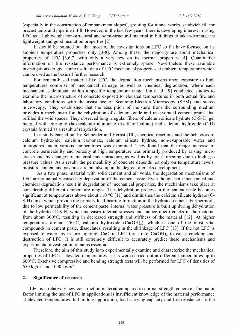
Md Azree Othuman Mydin & Y. C Wang CFD Letters Vol. 1(1) 2010
(especially in the construction of embankment slopes), grouting for tunnel works, sandwich fill for
precast units and pipeline infill. However, in the last few years, there is developing interest in using
LFC as a lightweight non-structural and semi-structural material in buildings to take advantage its
lightweight and good insulation properties [2].
It should be pointed out that most of the investigations on LFC so far have focused on its
ambient temperature properties only [3-8]. Among these, the majority are about mechanical
properties of LFC [3,6,7] with only a very few on its thermal properties [4]. Quantitative
information on fire resistance performance is extremely sparse. Nevertheless these available
investigations do give some useful data of LFC mechanical properties at ambient temperature which
can be used as the basis of further research.
For cement-based material like LFC, the degradation mechanisms upon exposure to high
temperatures comprise of mechanical damage as well as chemical degradation; where each
mechanism is dominant within a specific temperature range. Lin et al. [9] conducted studies to
examine the microstructure of concrete exposed to elevated temperatures in both actual fire and
laboratory conditions with the assistance of Scanning-Electron-Microscopy (SEM) and stereo
microscopy. They established that the absorption of moisture from the surrounding medium
provides a mechanism for the rehydration of calcium oxide and un-hydrated cement grains that
refilled the void spaces. They observed long irregular fibers of calcium silicate hydrate (C-S-H) gel
merged with ettringite (hexacalcium aluminate trisulfate hydrate) and calcium hydroxide (C-H)
crystals formed as a result of rehydration.
In a study carried out by Schneider and Herbst [10], chemical reactions and the behaviors of
calcium hydroxide, calcium carbonate, calcium silicate hydrate, non-evaporable water and
micropores under various temperatures was examined. They found that the major increase of
concrete permeability and porosity at high temperature was primarily produced by arising micro
cracks and by changes of material inner structure, as well as by crack opening due to high gas
pressure values. As a result, the permeability of concrete depends not only on temperature levels,
moisture content and gas pressure but also upon the degree of cracks development.
As a two phase material with solid cement and air voids, the degradation mechanisms of
LFC are principally caused by deprivation of the cement paste. Even though both mechanical and
chemical degradation result in degradation of mechanical properties, the mechanisms take place at
considerably different temperature ranges. The dehydration process in the cement paste becomes
significant at temperatures above about 110 °C [11] and diminishes the calcium silicate hydrate (C-
S-H) links which provide the primary load-bearing formation in the hydrated cement. Furthermore,
due to low permeability of the cement paste, internal water pressure is built up during dehydration
of the hydrated C-S-H, which increases internal stresses and induce micro cracks in the material
from about 300°C, resulting in decreased strength and stiffness of the material [12]. At higher
temperatures around 450°C, calcium hydroxide (Ca(OH)2), which is one of the most vital
compounds in cement paste, dissociates, resulting in the shrinkage of LFC [13]. If the hot LFC is
exposed to water, as in fire fighting, CaO in LFC turns into Ca(OH)2 to cause cracking and
destruction of LFC. It is still extremely difficult to accurately predict these mechanisms and
experimental investigation remains essential.
Therefore, the aim of this study is to experimentally examine and characterize the mechanical
properties of LFC at elevated temperatures. Tests were carried out at different temperatures up to
600°C. Extensive compressive and bending strength tests will be performed for LFC of densities of
650 kg/m3 and 1000 kg/m
3.
2. Significance of research
LFC is a relatively new construction material compared to normal strength concrete. The major
factor limiting the use of LFC in applications is insufficient knowledge of the material performance
at elevated temperatures. In building application, load carrying capacity and fire resistance are the
255
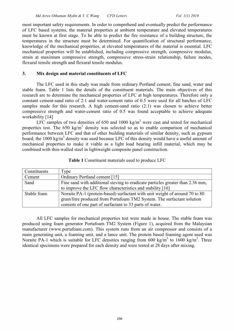
Md Azree Othuman Mydin & Y. C Wang CFD Letters Vol. 1(1) 2010
most important safety requirements. In order to comprehend and eventually predict the performance
of LFC based systems, the material properties at ambient temperature and elevated temperatures
must be known at first stage. To be able to predict the fire resistance of a building structure, the
temperatures in the structure must be determined. For quantification of structural performance,
knowledge of the mechanical properties, at elevated temperatures of the material is essential. LFC
mechanical properties will be established, including compressive strength, compressive modulus,
strain at maximum compressive strength, compressive stress-strain relationship, failure modes,
flexural tensile strength and flexural tensile modulus.
3. Mix design and material constituents of LFC
The LFC used in this study was made from ordinary Portland cement, fine sand, water and
stable foam. Table 1 lists the details of the constituent materials. The main objectives of this
research are to determine the mechanical properties of LFC at high temperatures. Therefore only a
constant cement-sand ratio of 2:1 and water-cement ratio of 0.5 were used for all batches of LFC
samples made for this research. A high cement-sand ratio (2:1) was chosen to achieve better
compressive strength and water-cement ratio of 0.5 was found acceptable to achieve adequate
workability [14]
LFC samples of two densities of 650 and 1000 kg/m3 were cast and tested for mechanical
properties test. The 650 kg/m3 density was selected so as to enable comparison of mechanical
performance between LFC and that of other building materials of similar density, such as gypsum
board; the 1000 kg/m3 density was used because LFC of this density would have a useful amount of
mechanical properties to make it viable as a light load bearing infill material, which may be
combined with thin-walled steel in lightweight composite panel construction.
Table 1 Constituent materials used to produce LFC
Constituents Type
Cement Ordinary Portland cement [15]
Sand Fine sand with additional sieving to eradicate particles greater than 2.36 mm,
to improve the LFC flow characteristics and stability [16]
Stable foam Noraite PA-1 (protein-based) surfactant with unit weight of around 70 to 80
gram/litre produced from Portafoam TM2 System. The surfactant solution
consists of one part of surfactant to 33 parts of water.
All LFC samples for mechanical properties test were made in house. The stable foam was
produced using foam generator Portafoam TM2 System (Figure 1), acquired from the Malaysian
manufacturer (www.portafoam.com). This system runs from an air compressor and consists of a
main generating unit, a foaming unit, and a lance unit. The protein based foaming agent used was
Noraite PA-1 which is suitable for LFC densities ranging from 600 kg/m3 to 1600 kg/m
3. Three
identical specimens were prepared for each density and were tested at 28 days after mixing.
256

Md Azree Othuman Mydin & Y. C Wang CFD Letters Vol. 1(1) 2010
Figure 1. Portafoam TM2 foam generator system.
4. Test methods
A variety of test methods may be used to obtain different aspects of mechanical properties
of materials at high temperatures, including the stressed test, the unstressed test, and the unstressed
residual strength test [17]. In this research, the unstressed test method was adopted for convenience.
In the unstressed test, the sample is heated, without preload, at a steady rate to the predetermined
temperature. While maintaining the target temperature, load is applied at a prescribed rate until
sample failure. Because the temperature is unchanged, the test is also referred to as steady state test,
as opposed to transient test in which the specimen temperature changes with time.
4.1 Heating of specimens
Electric furnace was used for heating the LFC specimens to the various steady-state
temperatures (100°C, 200°C, 300°C, 400°C, 500°C and 600°C). The furnace temperature exposure
profiles were produced by a programmable microprocessor temperature controller attached to the
furnace power supply and monitored by a Type K thermocouple located in the furnace chamber.
Pre-testing checking of the furnaces showed that the furnace controller and furnace power system
could maintain furnace operating temperatures within ±1°C over the test range.
4.2 Compression Test
The compressive strength tests were carried out on 100 x 200 mm cylinders. To monitor the
strain behaviour at ambient temperature during loading, two strain gauges were fitted on each
sample for the ambient test only. Since no strain measurement was made at elevated temperatures,
the ambient temperature strain measurements were used to confirm that the strain calculated based
on the displacement of the loading platen was of sufficient accuracy. Four Type K thermocouples
were installed in the central plane of each cylinder specimen. Loading was applied using an ambient
temperature compression machine (Figure 2) after removing the test samples from the furnace
(Figure 3). To minimise heat loss from the specimen to atmosphere, each specimen was wrapped
with insulation sheets immediately after being removed from the electric furnace. For each set of
test, three replicate tests were carried out to check consistency of the results.
Holding tank
Main generating
unit
Lance unit
257

Md Azree Othuman Mydin & Y. C Wang CFD Letters Vol. 1(1) 2010
Figure 2. Compression test using ambient temperature machine
Figure 3. High temperature electric furnace with specimens
4.3 Three point bending test
For convenience in this study, the three point bending test was carried out. The preparation of
samples followed a similar procedure as delineated above for the compression tests. The specimens
were rectangular parallelepipeds of height (h) 25 mm, width (w) 125 mm and length (l) 350 mm. As
shown in Figure 4, the LFC specimen was simply supported and was subjected to point load at the
centre point. The length between the supports was Ls = 200 mm, giving a Ls/h aspect ratio of 8 and
sufficient to ensure predominance of bending behaviour. The load-deflection was recorded for the
evaluation of flexural tensile strength.
258

Md Azree Othuman Mydin & Y. C Wang CFD Letters Vol. 1(1) 2010
Figure 4. Three point bending test set up and specimen dimensions
4.4 Porosity measurements
The porosity of LFC was determined by using the Vacuum Saturation Apparatus [18]. The porosity
was calculated using the following equation:
100)(
)(×
−
−=
watsat
drysat
WW
WWε …..(1)
where ε is the porosity (%), Wsat is the weight in air of saturated sample, Wwat is the weight in water
of saturated sample and Wdry is the weight of oven-dried sample.
5. Results and discussion
5.1 Porosity of LFC
Usually, the porosity of cement based material changes when the temperature increases. These
changes in porosity can be characterized by considering phase changes in the concrete at different
temperatures. Figure 5 presents the total porosity for each mix as a function of the temperature. LFC
of both densities experienced a slight monotonous increase in porosity with temperature. The initial
porosity for 650 and 1000 kg/m3 density was 74.8% and 50.0% respectively. Between 200°C and
300°C, the porosity increased considerably for the higher density LFC while the increase was more
moderate for the lower density LFC due to decomposition of the different amounts of calcium
silicate hydrate gel and sulfoaluminate. At 300°C, the measured porosity for 650 and 1000 kg/m3
density was 75.5% and 51.9% correspondingly. For temperatures beyond 400°C, the measured
porosity showed some increase corresponding to the decomposition of calcium hydroxide to form
calcium oxide. At 600°C, the porosity was 76.3% and 53.7% for 650 and 1000 kg/m3 respectively.
Nevertheless, in general, due to the high porosity at ambient temperature, LFC may be considered
to have constant porosity at various elevated temperatures.
259

Md Azree Othuman Mydin & Y. C Wang CFD Letters Vol. 1(1) 2010
40
50
60
70
80
90
100
0 100 200 300 400 500 600
Temperature (°C)
Po
rosi
ty (
%)
650 kg/m3
1000 kg/m3
`
Figure 5. Porosity of LFC as a function of temperature
Figures 6 show the pore size of LFC determined through image analysis tool which illustrate
images of the internal structure of the 1000 kg/m3 and 650 kg/m
3 density LFC at ambient
temperature. From Figures 6, it can be seen that the void sizes are not uniform and the average void
size is primarily a function of the LFC density. The same analysis of the images was also done for
both densities after being exposed to high temperatures and the results indicate that the void size did
not change much from that at ambient temperature.
260

Md Azree Othuman Mydin & Y. C Wang CFD Letters Vol. 1(1) 2010
(a) 650 kg/m
3 density
(b) 1000 kg/m
3 density
Figure 6. Pore sizes of LFC
5.2 Compressive strength of LFC
Figure 7 and Figure 8 illustrate the compressive strength and normalized compressive strength of
LFC as a function of temperature. It can be seen from Figures 7 and 8 that, for both densities, the
LFC compressive strength decreased with temperature. On initial heating, the LFC made with
Ordinary Portland Cement lost the absorbed, evaporable (free) water and then the chemically bound
water. The loss of water would induce micro cracking resulting in some reduction in compressive
strength. The compressive strength decreased slowly between 90°C to 170°C which due to the
release of free water and some of the chemically bound water. The decrease in compressive strength
between 20°C and 150°C corresponds to a reduction of the cohesion of the Van der Waal forces
between the calcium silicate hydrate layers [18]. This decreases the surface energy of calcium
silicate hydrate and leads to the formation of silanol groups (Si–OH: OH–Si) that presents weaker
bonding strength. However, because this change only affects the concrete superficially, the
reduction in concrete strength is not significant and the compressive strength of the LFC samples at
200°C still retained about 94% of the original unheated value. Between 200 °C and 400°C,
decomposition of C-S-H gel and the sulfoaluminate phases caused cracks in the specimens [13].
These cracks had significant effects on the compressive strength of LFC [20]. At 400 °C, the LFC
strength retained only about 75% of its initial value for both densities. Further degradation and loss
of strength continued to take place at high temperatures. At temperature of 600°C, the LFC retained
only about 40% of the original strength for both densities. Since the compositions of both densities
261

Md Azree Othuman Mydin & Y. C Wang CFD Letters Vol. 1(1) 2010
of LFC are identical, except for increased pores in the lower density LFC, it is not surprising that
the normalised strength – temperature relationships of LFC of both densities are almost the same.
0.0
1.0
2.0
3.0
4.0
5.0
6.0
0 100 200 300 400 500 600
Temperature (°C)
Co
mp
ress
ive S
tren
gth
(0
/mm
2)
650 kg/m3
1000 kg/m3
Figure 7. Compressive strength of LFC as a function of temperature
0.0
0.2
0.4
0.6
0.8
1.0
1.2
0 100 200 300 400 500 600
Temperature (°C)
0o
rm
ali
zed
Co
mp
ress
ive S
tren
gth
650 kg/m3
1000 kg/m3
`
Figure 8. Normalized compressive strength of LFC as a function of temperature
262
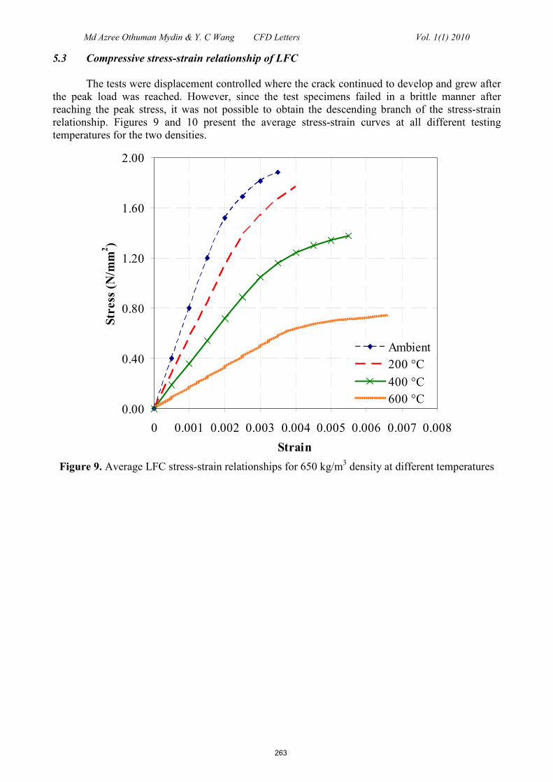
Md Azree Othuman Mydin & Y. C Wang CFD Letters Vol. 1(1) 2010
5.3 Compressive stress-strain relationship of LFC
The tests were displacement controlled where the crack continued to develop and grew after
the peak load was reached. However, since the test specimens failed in a brittle manner after
reaching the peak stress, it was not possible to obtain the descending branch of the stress-strain
relationship. Figures 9 and 10 present the average stress-strain curves at all different testing
temperatures for the two densities.
0.00
0.40
0.80
1.20
1.60
2.00
0 0.001 0.002 0.003 0.004 0.005 0.006 0.007 0.008
Strain
Str
ess
(0
/mm
2)
Ambient
200 °C
400 °C
600 °C
Figure 9. Average LFC stress-strain relationships for 650 kg/m
3 density at different temperatures
263

Md Azree Othuman Mydin & Y. C Wang CFD Letters Vol. 1(1) 2010
0.0
1.0
2.0
3.0
4.0
5.0
6.0
0 0.001 0.002 0.003 0.004 0.005 0.006
Strain
Str
ess
(0
/mm
2)
Ambient
200 °C
400 °C
600 °C
Figure 10. Average LFC stress-strain relationships for 1000 kg/m
3 density at different temperatures
It can be seen from Figures 9 and 10 that for both densities at all temperature levels, the
ascending branch was linear for stress up to 75% of the peak strength. The strain corresponding to
the peak strength increased at increasing temperatures. For LFC of 650 kg/m3 density, the
maximum strains were 0.0034, 0.0039, 0.0055 and 0.0066 at ambient temperature, 200°C, 400°C
and 600°C respectively; for the 1000 kg/m3 density, the corresponding values were 0.0024, 0.0029,
0.0039 and 0.0048 at ambient, 200°C, 400°C and 600°C respectively. The increase in strain results
from opening of cracks initiated by the heating at higher temperatures.
5.4 Modulus of elasticity of LFC in compression
Figures 11 and 12 demonstrate the changes in modulus of elasticity of LFC in compression
as a function of temperature. The modulus of elasticity was taken as the secant modulus at the point
where the material changed from elastic to plastic behavior from the experimental compressive
stress–strain curve. Compared to the reduction in LFC strength, the reduction in elastic modulus is
greater. Both figures show that the loss in modulus of elasticity began immediately upon heating
when the samples began to dry. The modulus of elasticity at 200°C, 400°C and 600°C was
respectively about 75%, 40% and 25% of the original value for both densities. As with changes in
normalised strengths of LFC of both densities at elevated temperatures, the normalised modulus of
elasticity of LFC of both densities at the same temperature are almost the same.
264

Md Azree Othuman Mydin & Y. C Wang CFD Letters Vol. 1(1) 2010
0.0
0.5
1.0
1.5
2.0
2.5
3.0
3.5
0 100 200 300 400 500 600
Temperature (°C)
Co
mp
ress
ive M
od
ulu
s (k
0/m
m2)
650 kg/m3
1000 kg/m3
`
Figure 11 Compressive modulus of LFC as a function of temperature
0.0
0.2
0.4
0.6
0.8
1.0
1.2
0 100 200 300 400 500 600
Temperature (°C)
0o
rm
ali
zed
Co
mp
ress
ive M
od
ulu
s
650 kg/m3
1000 kg/m3
Figure 12 Normalized compressive modulus of LFC as a function of temperature
265
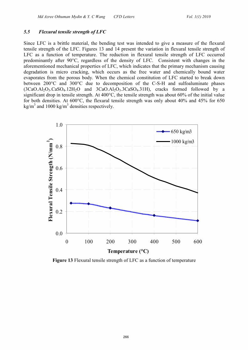
Md Azree Othuman Mydin & Y. C Wang CFD Letters Vol. 1(1) 2010
5.5 Flexural tensile strength of LFC
Since LFC is a brittle material, the bending test was intended to give a measure of the flexural
tensile strength of the LFC. Figures 13 and 14 present the variation in flexural tensile strength of
LFC as a function of temperature. The reduction in flexural tensile strength of LFC occurred
predominantly after 90°C, regardless of the density of LFC. Consistent with changes in the
aforementioned mechanical properties of LFC, which indicates that the primary mechanism causing
degradation is micro cracking, which occurs as the free water and chemically bound water
evaporates from the porous body. When the chemical constitution of LFC started to break down
between 200°C and 300°C due to decomposition of the C-S-H and sulfoaluminate phases
(3CaO.Al2O3.CaSO4.12H2O and 3CaO.Al2O3.3CaSO4.31H), cracks formed followed by a
significant drop in tensile strength. At 400°C, the tensile strength was about 60% of the initial value
for both densities. At 600°C, the flexural tensile strength was only about 40% and 45% for 650
kg/m3 and 1000 kg/m
3 densities respectively.
0.0
0.2
0.4
0.6
0.8
1.0
0 100 200 300 400 500 600
Temperature (°C)
Fle
xu
ra
l T
en
sile
Str
en
gth
(0
/mm
2)
650 kg/m3
1000 kg/m3
Figure 13 Flexural tensile strength of LFC as a function of temperature
266

Md Azree Othuman Mydin & Y. C Wang CFD Letters Vol. 1(1) 2010
0.0
0.2
0.4
0.6
0.8
1.0
1.2
0 100 200 300 400 500 600
Temperature (°C)
0o
rm
ali
zed
Fle
xu
ra
l T
en
sile
Str
en
gth
650 kg/m3
1000 kg/m3
Figure 14 Normalized flexural tensile strength of LFC as a function of temperature
5.6 Flexural tensile modulus of LFC
Figures 15 and 16 illustrate the changes in flexural modulus of LFC as a function of temperature
and comparison of the normalized flexural modulus with the normalized compressive modulus
obtained from the cylinder tests. Although there are some differences, the variation of the
normalized compressive modulus and normalized flexural modulus values are very similar for both
densities at various temperatures.
267

Md Azree Othuman Mydin & Y. C Wang CFD Letters Vol. 1(1) 2010
0.0
0.5
1.0
1.5
2.0
2.5
3.0
3.5
0 100 200 300 400 500 600
Temperature (°C)
Fle
xu
ral
tensi
le m
odu
lus
(k0
/mm
2)
650 kg/m3
1000 kg/m3
`
Figure 15 Flexural tensile modulus of LFC as a function of temperature
0.0
0.2
0.4
0.6
0.8
1.0
1.2
0 100 200 300 400 500 600
Temperature (°C)
0o
rm
ali
zed
co
mp
ress
ive a
nd
fle
xura
l m
od
ulu
s
650 kg/m3 (compressive modulus)
1000 kg/m3 (compressive modulus)
650 kg/m3 (flexural modulus)
1000 kg/m3 (flexural modulus)
Figure 16 Comparison of normalized compressive modulus and flexural tensile modulus of LFC as
a function of temperature
268

Md Azree Othuman Mydin & Y. C Wang CFD Letters Vol. 1(1) 2010
6.0 Conclusions
This paper has presented the results of a series of experimental studies to study the
mechanical properties of LFC at elevated temperatures. Compressive cylinder tests and three point
bending tests were carried out for two different LFC densities at various temperatures from ambient
up to 600oC. The mechanical properties included compressive cylinder strength, compressive
modulus of elasticity, compressive stress-strain relationship, strain at the maximum compressive
stress, porosity, flexural bending strength and modulus of elasticity.
The experimental results consistently demonstrate that the loss in stiffness for cement based
material such as LFC at elevated temperatures occurs predominantly after about 90°C, regardless of
density. This indicates that the primary mechanism causing stiffness degradation is microcracking,
which occurs as water expands and evaporates from the porous body. As expected, reducing the
density of LFC reduces its strength and stiffness. However, for LFC of different densities, the
normalised strength and stiffness (ratio of elevated temperature value to ambient temperature value)
–temperature relationships are very similar.
Acknowledgments
Acknowledgement is made to the funding bodies of author PhD studies, University Science
Malaysia and Ministry of Higher Education Malaysia. The author would also acknowledge the
assistance rendered by academic members and staff of the School of Mechanical, Aerospace and
Civil Engineering with particular thanks goes to the technical staff members Mr. Jim Gee, Mr. John
Mason, Mr. Bill Storey, Mr. Paul Townsend and Mr. Paul Nedwell for their invaluable.
References
1. Van Deijk, S. Foamed Concrete. A Dutch View, BRE, 1992, pp. 2-8.
2. Kearsley, E. P., and Mostert, H. F., Opportunities for expanding the use of foamed concrete in
the construction industry. In: Dhir, R. K., Newlands, M. D., McCarthy, A., Editors; Use of
foamed concrete in construction, Thomas, London, 2005, p. 29-36.
3. Dransfield, J. M., Foamed concrete: Introduction to the product and its properties. One day
awareness seminar on ‘Foamed concrete: properties, applications and potential’ held at
University of Dundee, Scotland, 2000, p. 1-11.
4. Giannakou, A., and Jones, M. R., Potentials of foamed concrete to enhance the thermal
performance of low rise dwellings. In: Dhir, R. K., Hewelett, P. C., Csetenyi, L. J., Editors;
Innovations and development in concrete materials and construction, Thomas Telford, United
Kingdom, 2002, p. 533-544.
5. Hamidah, M. S,, Azmi, I., Ruslan, M. R. A., Kartini, K., and Fadhil, N. M., Optimisation of
foamed concrete mix of different sand-cement ratio and curing conditions. In: Dhir, R. K.,
Newlands, M. D., McCarthy, A., Editors; Use of foamed concrete in construction, Thomas,
London, 2005, p. 37-44.
6. Jones, M. R., Foamed concrete for structural use. In: Proceedings of one day seminar on
foamed concrete: properties, applications and latest technological developments,
Loughborough University, 2001, p. 27-60.
7. Jones, M. R., and McCarthy, A., Behaviour and assessment of foamed concrete for
construction applications. In: Dhir, R. K., Newlands, M. D., McCarthy, A., Editors; Use of
foamed concrete in construction, Thomas, London, 2005, p. 61-88.
8. Nambiar, E. K. K., and Ramamurthy, K., Air-void characterization of foam concrete. J.
Cement Concr. Res., 2007. 37(2): p. 221-230.
9. Lin, W. M., Lina, T. D., and Powers-Couche, L. J., Microstructures of fire-damaged concrete.
Journal of American Concrete Institute Materials, 1996. 93(3): p. 199-205.
269

Md Azree Othuman Mydin & Y. C Wang CFD Letters Vol. 1(1) 2010
10. Schneider, U., and Herbst, H. Permeability and porosity of concrete at high temperature.
Technical report 403, Deutscher Ausschuss für Stahlbeton, Berlin, In German, 1989.
11. Khoury, G. A., Majorana, C. E., Pesavento, F., and Schrefler, B. A. Modelling of heated
concrete. Mag. Concr. Res., 2002. 54(2): p 77–101.
12. Hertz, K. D. Concrete strength for fire safety design. Mag. Concr. Res., 2005. 57(8): p. 445-
453.
13. Taylor, H. F. W. Cement Chemistry. London: Academic Press, 1992.
14. Md Azree, O. M. Effect of using additives to the compressive strength of lightweight foamed
concrete. Master Dissertation, School of Housing, Building and Planning, University of
Science Malaysia, Penang, 2004.
15. BS EN 197-1. Cement: Composition, Specifications and conformity criteria for low heat
common cements. British Standards Institution, London, 2000.
16. BS EN 12620. Aggregates for Concrete. British Standards Institution, London, 2002.
17. Phan, L. T., and Carino N. J. Code provisions for high strength concrete strength temperature
relationship at elevated temperatures. J. of Mater. Struct., 2003. 36(2): p. 91-98.
18. Cabrera, J. G., and Lynsdale, C. J. A new gas permeameter for measuring the permeability of
mortar and concrete. Mag. Concr. Res., 1998. 40(144): p. 177-182.
19. Khoury, G. A., Compressive strength of concrete at high temperatures: A reassessment. Mag.
Concr. Res., 1992. 44(161): p. 291-309.
20. Ai, H., Young, J.F., and Scherer, G. W. Thermal expansion kinetics: Method to measure
permeability of cementitious materials: II, application to hardened cement pastes. J. Am.
Ceram. Soc., 2001. 84(2): 385-391.
270

Thin-Walled Structures ] (]]]]) ]]]–]]]
Contents lists available at ScienceDirect
Thin-Walled Structures
0263-82
doi:10.1
n Corr
E-m
journal homepage: www.elsevier.com/locate/tws
Structural performance of lightweight steel-foamed concrete–steelcomposite walling system under compression
Md Azree Othuman Mydin, Y.C. Wang n
School of Mechanical, Aerospace and Civil Engineering, The University of Manchester, PO Box 88, Manchester M60 1QD, UK
a r t i c l e i n f o
Article history:
Received 25 May 2010
Accepted 17 August 2010
Keywords:
Composite walling
Sandwich panel
Thin-walled
Foamed concrete
Structural performance
Loadbearing wall
31/$ - see front matter & 2010 Elsevier Ltd. A
016/j.tws.2010.08.007
esponding author. Tel.: +44 161 3068968; fa
ail address: [email protected] (Y.
a b s t r a c t
This paper presents the results of an experimental and analytical investigation on the structural
behaviour of a composite panel system consisting of two outer skins of profiled thin-walled steel plates
with lightweight foamed concrete (LFC) core under axial compression. The gross dimensions of the test
specimens were 400 mm�400 mm�100 mm. A total of 12 tests were carried out, composed of two
duplicates of 6 variants which were distinguished by two steel sheeting thicknesses (0.4 mm and
0.8 mm) and three edge conditions of the sheeting. The density of LFC was 1000 kg/m3. Experimental
results include failure modes, maximum loads and load-vertical strain responses. In analysis, full bond
between the steel sheets and the concrete core was assumed and the LFC was considered effective in
restraining inward buckling of the steel sheets. Using the effective width method for the steel sheets,
the load carrying capacities of the test specimens were calculated and compared with the experimental
results. It was found that a combination of the Uy and Bradford plate local buckling coefficients with the
Liang and Uy effective width formulation produced calculation results in good agreement with the
experimental results. Finally, a feasibility study was undertaken to demonstrate the applicability and
limit of this new composite walling system in low rise construction.
& 2010 Elsevier Ltd. All rights reserved.
1. Introduction
Lightweight foamed concrete (LFC) is a cellular materialcomposed of cement–sand matrix enclosing a large number ofsmall pores roughly 0.1–1.0 mm size, uniformly distributed ineither a matrix of aggregate and cement paste or cement pastealone. The essential advantage of LFC to the field of concretetechnology is the capability to control its density over a widerange. LFC densities of 400–1600 kg/m3 can be attained byappropriate control in dosage of foam for application as structural,partition and insulation material. Although LFC has primarilybeen utilized as a void filling and insulation material, it is possibleto use LFC as structural loadbearing material in low loadbearingsystems such as walls in low-rise residential buildings. LFCconstruction would be particularly attractive if precast LFCmembers can be made to be carried by manual workers on sitewithout the use of machinery.
The authors have recently conducted research studies toobtain data of thermal and mechanical properties of LFC [1,2].We have found that due to its porous internal structure, LFC hasvery low thermal conductivity, making it a suitable material forbuilding use as insulating or fire resisting material. LFC can also bemade to have a reliable amount of compressive resistance, making
ll rights reserved.
x: +44 161 306 4646.
C. Wang).
271
it possible to use LFC as loadbearing material. However, theauthors’ research on compressive properties of LFC indicated thatLFC suffered from brittle failure. Therefore, a suitable method ofusing LFC in loadbearing construction would be to use it incomposite action with steel, which has high ductility. Thisresearch explores the use of LFC in composite action with steelsheeting in lightweight composite walling construction. ShouldLFC be cast in-situ, the thin steel sheeting can be used asformwork during construction. Because of the low density of LFC,the pressure on the steel sheeting during construction would bemuch lower than using normal strength concrete, allowing thinsteel sheeting to be used.
Before such a system can be used in practice, it is necessary tocarry out fundamental research to thoroughly investigate itsbehaviour. This paper will present the results of an experimentaland analytical study of the compressive behaviour of shortcomposite panel made of profiled thin steel sheeting as the facingand LFC as the core material.
2. Experiments
The experiments were designed to provide information on theload deformation response and failure modes of the specimens.The objective of the experiments was to enable development of acalculation method.

M.A. Othuman Mydin, Y.C. Wang / Thin-Walled Structures ] (]]]]) ]]]–]]]2
2.1. Geometrical descriptions of specimen
The dimensions of the test specimens were 400 mm high�400mm wide�100 mm thick. The short height of the specimens would
120mm
120mm
400mm
45mm 50mm 50mm
100mm
10mm
400mm
foamed concrete core
profiled steel sheeting
400mm
10mm intermediate bolts
Fig. 1. Details of prototype composite walling.
Fig. 2. Steel sheeting edge conditions: (a) no stopping edge, (b
2
mean that failure of the specimens would be governed by cross-sectional capacity. A total of 12 prototype specimens were testedunder axial compression. These 12 specimens consisted of twoduplicates of 6 types, being two steel thicknesses (0.4 and 0.8 mm) incombination with three edge conditions of the steel sheeting. Fig. 1shows details of the prototype specimen. The profiled steel sheetingwas made in-house from plain sheeting of 0.4 or 0.8 mm thickness byfly press. The two profiled steel facings were connected using6 mm�10 mm bolts and nuts. Referring to Fig. 2, the steel sheetingcould have one of the three edge conditions: (a) the steel sheets donot cover the LFC panel thickness (referred to as no stopping edge),(b) the steel sheets cover the LFC panel thickness but are not joined(referred to as with stopping edges), (c) the steel sheets cover the LFCpanel thickness and are joined by welding (referred to as weldedstopping edge). These three steel sheeting edge conditions wereinvestigated to assess the influence of the steel sheeting in restrainingthe LFC to improve its ductility.
2.2. Casting, curing and instrumentation
All twelve specimens (Fig. 3) were cast in house on the sameday so that the LFC core would have the same design strength. TheLFC used in this study was made from ordinary Portland cement,fine sand, water and stable foam [3,4]. Table 1 lists details of theconstituent materials. The cement–sand ratio was 2:1 and thewater–cement ratio was maintained at 0.5.
The stable foam was produced using foam generator Porta-foam TM2 System, obtained from a Malaysian manufacturer(www.portafoam.com). This system runs from an air compressorand consists of a main generating unit, a foaming unit and a lanceunit. The foaming agent used was Noraite PA-1 (protein based),which is suitable for LFC densities ranging from 600 to 1600 kg/m3.Noraite PA-1 comes from natural sources and has a weight ofaround 80 g/litre and expands about 12.5 times when used withthe Portafoam foam generator.
) with stopping edge and (c) with welded stopping edge.
72

M.A. Othuman Mydin, Y.C. Wang / Thin-Walled Structures ] (]]]]) ]]]–]]] 3
LFC with density of 1000 kg/m3 was chosen as it was found tohave a useful amount of mechanical properties to construct alightweight loadbearing walling system when in composite actionwith the profiled cold-formed thin-walled steel sheeting. ThreeLFC cubes and three cylinders were also cast on the day thecomposite panels were made. Additional two sets of threeidentical tests were also conducted to determine the strength ofLFC core alone without any steel plate. Fig. 4 shows the shapes of
Fig. 3. LFC filled profiled cold-formed thin-walled steel.
Table 1Constituent materials used to produce LFC.
Constituents Type
Cement Ordinary Portland cement conforming to BSEN 197–1 [1]
Sand Fine sand conforming to BS EN 12620, with additional sieving to
eradicate particles greater than 2.36 mm, to improve the LFC
flow characteristics and stability [2]
Stable foam Noraite PA-1 (protein based) foaming agent with weight of
around 80 g/litre produce from Portafoam TM2 System.
Fig. 4. Dimensions of the two additional LFC core samples
273
these two additional sets. These tests were carried out to establishthe LFC core strength contribution factor when in compositeaction with the steel sheeting. These two shapes were used todetermine the effects of profiling on compressive strength of thecore, as observed by Wright [5]. LFC was poured vertically similarto the direction of loading and the test samples were naturallycured in the indoor climate of the concrete lab. The compositepanel was tested at the 28th day after casting.
A number of strain gauges were placed on the specimens andFig. 5 shows their locations on a sample. In all cases, the straingauges were at mid-height (h/2) of the specimen.
2.3. Test set-up
The specimens were loaded in axial compression and the testwas carried out in a universal compression testing machine with amaximum capacity of 2500 kN after 28 days of casting (Fig. 6).The tests were displacement controlled. The top and bottom ofthe specimens were ground flat prior to testing so as to ensureequal load distribution. In addition to the strain gauges on the
: (a) rectangular LFC panel and (b) profiled LFC panel.
120mm
120mm
400mm
400mm
S1,S3 S2,S4B1,B3 B2,B4
Fig. 5. Strain gauge arrangement.

Table 3Summary of test results.
Test no. Reference Steel thickness (mm) Ultimate strength (kN)
1 NSE1 0.4 161
M.A. Othuman Mydin, Y.C. Wang / Thin-Walled Structures ] (]]]]) ]]]–]]]4
sample, the displacement of the loading platen was also recordedto measure axial deformation of the specimen. Observations weremade on general behaviour including cracking of concrete,buckling of sheeting and failure mode.
2.4. Material properties
Three concrete cubes and 3 cylinders were cast and tested on thesame days as the composite walling specimens. The cube tests after28 days gave an average strength of 5.9 N/mm2 and the cylindertests provided an average strength of 5.1 N/mm2. The test results aregiven in Table 2 and they are quite consistent. Table 2 also gives theresults of the additional tests on the LFC panels. Data from the steelsheeting supplier gave yield strength of 280 N/mm2 and a modulusof elasticity of 200,000 N/mm2.
The strength ratio given in Table 2 indicates that the compressivestrength of LFC was influenced by the shape and size of thespecimens, which conforms to the observed behaviour of the normalstrength of the concrete. The average cylinder strength and solidpanel strength were 15% and 30% lower than the cube strength,respectively. The strength of the profiled panel was slightly smallerthan the strength of the solid panel as found by Wright [5].
2 NSE2 169
3 NSE3 0.8 240
4 NSE4 247
5 WSE1 0.4 175
6 WSE2 187
7 WSE3 0.8 263
8 WSE4 272
9 WE1 0.4 189
10 WE2 207
11 WE3 0.8 285
12 WE4 302
NSE¼no stopping edge; WSE¼with stopping edge; WE¼welded edge
3. Test results and observations
Table 3 lists the ultimate strength (maximum load) of eachspecimen. Except for tests 9 and 10 which show a difference ofabout 10%, other duplicate tests reached very similar ultimatestrengths. Figs. 7–12 present the load versus mid-height verticalstrain relationships for the six types of specimens. The differentstrain gauges (S1–S4 and B1–B4) recorded very similar data soonly data from one of each sets are considered (S1 on the steel
Fig. 6. Axial compression test set-up.
Table 2Variation of compressive strength of LFC core for different shapes and dimensions.
Shapes Dimension (mm) Compressive strength (N/mm2)
Test 1 Test 2
Cube 100�100�100 5.7 6.2
Cylinder 100ø�200 4.9 5.1
Solid panel 400�400�100 4.1 4.0
Profiled panel 400�400�100 3.8 3.7
2
surface without any mechanical connectors, B1 on the steelsurface between the mechanical fasteners).
Figs. 7–12 indicate that in all cases, the strain gauge S1recorded more elastic strains than B1, indicating participation ofthe mechanical fasteners. In all cases, the test sample was able tosustain the maximum applied load for a considerable axialdeformation. The descending branch of all the load–strain curveswas gradual, indicating good ductility of the test specimen.
Table 3 shows that the ultimate strength of the specimens withstopping edge was about 10% higher than those without anystopping edge for both steel thicknesses. Panels with welded steeledges sustained on average 17% more load than those withoutstopping edge. In Section 4, it will be shown that the increase inthe strength can be attributed to the increase in the effectivewidth of the steel sheeting.
Average strength
(N/mm2)
Ratio of strength
to cube strength
Test 3
5.9 5.9 1.00
5.3 5.1 0.86
4.3 4.1 0.69
3.5 3.7 0.63
0
50
100
150
200
0 0.005 0.01 0.015 0.02 0.025Axial Strain
Axi
al L
oad
(kN
)
Test 1 (Point B1)
Test 1 (Point S1)
Test 2 (Point B1)
Test 2 (Point S1)
Test 1
Test 2
Fig. 7. Load versus mid-height strain relationships for the panel with 0.4 mm steel
thickness and no stopping edge.
74

0
50
100
150
200
0.000 0.005 0.010 0.015 0.020
Axial Strain
Axi
al L
oad
(kN
)
Test 5
Test 6 Test 5 (Point B1)
Test 5 (Point S1)
Test 6 (Point B1)
Test 6 (Point S1)
Fig. 9. Load versus mid-height strain relationships for the panel with 0.4 mm steel
thickness and with stopping edge.
0
50
100
150
200
250
300
0 0.005 0.01 0.015 0.02 0.025
Axial Strain
Axi
al L
oad
(kN
)
Test 3 (Point B1)
Test 3 (Point S1)
Test 4 (Point B1)
Test 4 (Point S1)
Test 3
Test 4
Fig. 8. Load versus mid-height strain relationships for the panel with 0.8 mm steel
thickness and no stopping edge.
0
50
100
150
200
250
300
0.000 0.005 0.010 0.015 0.020
Axial Strain
Axi
al L
oad
(kN
)
Test 7 (Point B1)
Test 7 (Point S1)
Test 8 (Point B1)
Test 8 (Point S1)
Test 7
Test 8
Fig. 10. Load versus mid-height strain relationships for the panel with 0.8 mm
steel thickness and with stopping edge.
0
50
100
150
200
250
510.010.0500.00
Axial Strain
Axi
al L
oad
(kN
)
Test 9 (Point B1)
Test 9 (Point S1)
Test 10 (Point B1)
Test 10 (Point S1)
Test 9
Test 10
Fig. 11. Load versus mid-height strain relationships for the panel with 0.4 mm
steel thickness and with welded edge.
0
50
100
150
200
250
300
350
510.010.0500.00
Axial Strain
Axi
al L
oad
(kN
)
Test 11
Test 12 Test 11 (Point B1)
Test 11 (Point S1)
Test 12 (Point B1)
Test 12 (Point S1)
Fig. 12. Load versus mid-height strain relationships for the panel with 0.8 mm
steel thickness and with welded edge.
0
50
100
150
200
250
300
350
30.020.010.00
Axial Strain
Axi
al L
oad
(kN
)
Test 1
Test 11
Test 5
Test 9Test 3
Test 7
Profiled panel without steel sheeting
`
Test 1 - 0.4mm (no stopping edge) Test 3 - 0.8mm (no stopping edge)Test 5 - 0.4mm (with stopping edge) Test 7 - 0.8mm (with stopping edge) Test 9 - 0.4mm (welded edge) Test 11 - 0.8mm (welded edge) Profiled panel without steel sheeting 1Profiled panel without steel sheeting 2
Fig. 13. Comparison of load versus mid-height strain (point B1) relationships of
the two steel sheeting thicknesses and three edge conditions and also with
profiled panels without steel sheeting.
M.A. Othuman Mydin, Y.C. Wang / Thin-Walled Structures ] (]]]]) ]]]–]]] 5
Fig. 13 compares the load versus mid-height strain (point B1)relationships of the two steel sheeting thicknesses and three edgeconditions, and also with profiled panels without steel sheeting.As expected, the ultimate load and axial stiffness of the compositepanel increases with increase in the steel thickness and improvededge condition. The most striking feature of Fig. 13 is that the use
275

M.A. Othuman Mydin, Y.C. Wang / Thin-Walled Structures ] (]]]]) ]]]–]]]6
of steel sheeting on both faces of the profiled LFC panelconsiderably increased the ductility of the panel for all the edgeconditions and steel thicknesses. The introduction of steelsheeting enables the panel to sustain a high proportion of itspeak load at increasing deformations. In contrast, for the profiledpanel without steel sheeting, both specimens failed in a brittlemanner after reaching the peak load and it was not possible toattain the descending branch of the load–strain relationship.
Fig. 14 shows a failed sample for all three edge conditions: (a)without stopping edge, (b) with stopping edge and (c) withwelded edge. The steel sheeting experienced local buckling beforefailure, but the LFC core of 1000 kg/m3 density was capable ofpreventing the panel from inward buckling. In all cases, failure ofthe panel was initiated by local buckling of the steel sheeting,followed by crushing of the LFC core. Although the steel sheetingprovided some ductility to the panel, the welded steel edges werenot able to provide much confinement effect to the LFC panel.There was no separation of the steel sheeting from the LFC coreuntil near failure, indicating that the mechanical fasteners were
Fig. 14. Failure mode for composite panel without stopping edge: (a) failure mode of
specimen with stopping edge and (c) failure mode of specimen with welded edge.
2
able to hold the steel sheeting and the LFC core together to enablethem to resist the applied load in composite action. Clearly, ifcomposite walling system using LFC is to be used in real projects,bond between the profiled steel sheeting and the LFC infill shouldbe considered. However, it is expected that because LFC would beless demanding owing to its lower strength than normal strengthconcrete, the steel sheeting used in composite walling systemsusing normal strength concrete would still be suitable.
4. Analytical results
As previously described, the panels can be considered to be incomposite action and the LFC core was able to prevent the steelsheeting from inward local buckling. Therefore, the test specimenswill be analysed as a conventional composite walling system.
Since the test panels were short (height to thickness ratio¼4),no global buckling was observed and the panel strength reachedthe cross-sectional resistance. Also experimental observation
panel without stopping edge with outward buckling of steel, (b) failure mode of
76

M.A. Othuman Mydin, Y.C. Wang / Thin-Walled Structures ] (]]]]) ]]]–]]] 7
indicates that there was little evidence (e.g. bulging of the steelsheeting) of any confinement effect on the LFC core provided bythe steel sheeting. Therefore, the ultimate resistance of the panel,Nu, may be calculated from
Nu ¼NsþNc ð1Þ
where Ns is the resistance of the steel sheeting and Nc theresistance of the LFC core. The following sections will discuss howNs and Nc may be obtained.
4.1. Steel sheeting resistance
4.1.1. Critical local buckling stress
The local buckling stress of the steel plate in concrete-filledsteel section is influenced by the width to thickness ratio,boundary condition, initial geometric imperfection and residualstresses induced by welding or cold-formed process [6]. For idealsteel plates, the critical elastic buckling stress can be determinedby the following equation [7]:
scr ¼kp2Es
12ð1�v2Þðb=tÞ2ð2Þ
where scr is the local buckling stress, k is the elastic bucklingcoefficient, which accounts for the effect of the plate aspect ratioand boundary condition on the critical buckling stress, Es is themodulus of elasticity of the steel, n is the Poisson’s ratio, b is thewidth of the plate and t is the thickness of the plate.
4.1.2. Plate buckling coefficient
The plate buckling coefficient of the steel section depends on theboundary condition. Therefore, the buckling coefficient is a functionof the boundary condition along the longitudinal edges and the typeof loading. The k values for various common boundary conditionsand loading cases are given by a few authors [8,9]. Gerard andBecker [8] summarized the buckling coefficient, k, as a function ofplate boundary condition and aspect ratio (a/b). Gerard and Becker’s
Table 5Effective width of steel plates in composite panel.
Steel Thickness (mm) Total effective width (be/b)
Uy and Bradford k value
Winter [10] Liang an
(1) (2)
No stopping edges
0.4 0.51 0.47
0.8 0.74 0.65
With stopping edges
0.4 0.49 0.46
0.8 0.74 0.66
Welded edges
0.4 0.54 0.49
0.8 0.82 0.71
Table 4Buckling coefficient of steel plates under compression.
Boundary condition Buckling coefficient, k
Gerard and Becker [8] Uy and Bradford [9]
S–F 0.425 0.8
S–S 4 5.6
S-F: simply supported–free, S–S: simply supported-simply supported.
277
results are based on steel plates in contact with rigid medium. Uyand Bradford [9] recently proposed a slightly different set of platebuckling coefficients for steel plates in contact with elastic medium,which would be more suitable to the current problem. For thecurrent research which has uniform distribution of compressivestress, the buckling coefficients are compared in Table 4.
4.1.3. Effective width
For thin-walled structures, the current design method is to usean effective width to account for local buckling. According toWinter [10], the effective width (beff) of a plate of width b can becalculated using the following equation:
beff
b¼
ffiffiffiffiffiffiffiffiffiffiffiffiffiffiffiffiffiffiffiffiffiffiffiffiffiffiffiffiffiffiffiffiffiffiffiffiffiffiffiffiffiffiffiffiffiffiffiffiffiffiffiffiffiffiscr
fy
� �1�0:22
ffiffiffiffiffiffiffiffiffiffiffiffiffiffiscr
fy
� �s" #vuut ð3Þ
where beff is the effective width, b is the original width, scr is thelocal buckling stress and fy is the yield stress. The yield stress fy,multiplied by the effective width gives the ultimate strength ofthe plate approximately.
Liang and Uy [6] conducted a theoretical study on the post-local buckling behaviour of steel plates in steel box columns filledwith concrete, by using the finite element method. They foundthat the post-local buckling characteristics of steel plates inconcrete filled thin-walled box columns have not been adequatelystudied theoretically and there is also lack of an efficient methodfor evaluating the initial local buckling loads of steel plates. Theyexamined the effective width methods for the ultimate strengthdesign of steel plates restrained by concrete and of short concrete-filled welded box columns in compression and proposed thefollowing two effective width equations:
beff
b¼ 0:675
scr
fy
� �1=3
for scr r fy ð4Þ
beff
b¼ 0:915
scr
scrþ fy
� �1=3
for sc 4 fy ð5Þ
The resistance of the steel sheeting can be calculated as
Ns ¼ beff tfy ð6Þ
4.2. Strength of LFC core
A study conducted by Wright [5] established that there was areduction in load carrying capacity in profiled concrete panelwhen compared to solid panel. He found that the extreme edges
Gerard and Becker k value
d Uy [6] Winter [10] Liang and Uy [6]
(3) (4)
0.44 0.43
0.67 0.60
0.43 0.41
0.67 0.59
0.47 0.45
0.74 0.66

0
100
200
300
400
500
0 0.2 0.4 0.6 0.8 1 1.2
Profile thickness (mm)
Axi
al lo
ad (k
N)
Winter effective width with Uy & Bradford k value
Liang & Uy effective width with Uy & Bradford k value
Winter effective width with Gerrard & Becker k value
Liang & Uy effective width with Gerrard & Becker k value
Test results
Fig. 16. Comparisons between predicted strengths and test results for composite
panel with stopping edge.
0
100
200
300
400
0 0.2 0.4 0.6 0.8 1 1.2Profile thickness (mm)
Axi
al lo
ad (k
N)
Winter effective width with Uy & Bradford k value
Liang & Uy effective width with Uy & Bradford k value
Winter effective width with Gerrard & Becker k value
Liang & Uy effective width with Gerrard & Becker k value
Test results
Fig. 15. Comparisons between predicted strengths and test results for composite
panel with no stopping edge.
M.A. Othuman Mydin, Y.C. Wang / Thin-Walled Structures ] (]]]]) ]]]–]]]8
of the profiled panel did not present a solid mass of concrete andthe extra bending stresses (due to any loading eccentricity ormaterial non-uniformity) must be carried by only that concrete inthe ribs of the profile. This reduces the load carrying capacity ofthe rib to resist the applied axial load.
Wright [5] then derived an empirical correction to calculatethe reduced concrete strength for uniform axial compression,where the reduction in concrete strength is assumed to be directlyproportional to the extent of void created by profiling thecompressed edge of the panel. A reduction factor, a, which isapplied to the concrete strength is given as follows:
a¼ 1�Avf
Acð7Þ
where Avf is the area of the profile voids on one face and Ac is the areaof concrete. For the tested samples, the calculated a value is 0.91.
The test results in Table 2 appear to confirm the findings byWright [5] where the compressive strength of the profiled LFCpanel was found to be lower than the concrete strength of thesolid panel. Therefore, an experimental correction (a reductionfactor in Eq. (6)) must be included when calculating the resistanceof the LFC core in the composite walling system.
Based on this result, the resistance of the LFC core in the proposedcomposite walling system can be determined as follows:
Nc ¼ 0:69Acfcua ð8Þ
The factor of 0.69 (see Table 2) takes into account the reducedstrength of LFC in a panel construction compared to the cubestrength of LFC, and it was determined by dividing the average solidpanel strength (4.1 N/mm2) by the cube strength (5.9 N/mm2). Withthe introduction of a calculated using Eq. 7 (0.91), Eq. (8) gives afinal factor of 0.63 which is the same as the experimental result inTable 2, obtained by dividing the LFC strength in the profiled panelby the LFC cube strength.
4.3. Load carrying capacity of composite wall panels
Based on the discussion in the last section, the load carryingcapacity of the composite wall panel in axial compression, takinginto consideration the effective width and concrete strengthreduction factor for profiled shape, can be calculated by using thefollowing equation:
Ns ¼ 0:63Acfcuþbeff tfy ð9Þ
Table 6Comparisons between predicted composite panel strengths and test results.
Ref. No. Predicted Strength (kN)
Gerard and Becker k value Uy and Bradford k value
Liang and Uy Winter Liang and Uy Winter
NSE1 169 171 174 177
NSE2
NSE3 245 259 256 273
NSE4
WSE1 177 179 182 187
WSE2
WSE3 270 288 286 306
WSE4
WE1 182 184 187 192
WE2
WE3 287 307 300 325
WE4
Mean, x
Standard deviation, s
2
Table 5 presents the total effective width of steel sheeting forthe two different thicknesses and the three different edgeconditions, using the aforementioned two different methods ofcalculating the plate buckling coefficient and two methods of
Ratio predicted/experiment
Gerard and Becker k value Uy and Bradford k value
Liang and Uy Winter Liang and Uy Winter
1.05 1.06 1.08 1.10
1.00 1.01 1.03 1.05
1.02 1.08 1.07 1.14
0.99 1.05 1.04 1.11
1.01 1.02 1.04 1.07
0.95 0.96 0.98 1.00
1.03 1.09 1.09 1.16
0.99 1.06 1.05 1.12
0.96 0.97 0.99 1.02
0.88 0.89 0.90 0.93
1.01 1.08 1.05 1.14
0.95 1.02 0.99 1.07
0.9867 1.0242 1.0258 1.0758
0.0458 0.0596 0.0532 0.0674
78

Fig. 18. Arrangement of LFC composite wall panels
0
100
200
300
400
500
0 0.2 0.4 0.6 0.8 1 1.2
Profile thickness (mm)
Axi
al lo
ad (k
N)
Winter effective width with Uy & Bradford k value
Liang & Uy effective width with Uy & Bradford k value
Winter effective width with Gerrard & Becker k value
Liang & Uy effective width with Gerrard & Becker k value
Test results
Fig. 17. Comparisons between predicted strengths and test results for composite
panel with welded edge.
M.A. Othuman Mydin, Y.C. Wang / Thin-Walled Structures ] (]]]]) ]]]–]]] 9
279
calculating the plate effective width. The total effective widthcoefficient is obtained as the sum of effective widths of all thesegments of the profiled steel sheeting divided by the total widthof the steel sheeting.
It is interesting to notice that if the same plate bucklingcoefficient is used, the two different effective width methods(compare (1) with (2) or (3) with (4)) give substantial differencesin the total effective width of the steel sheeting, with the Liang andUy [6] method (Eqs. (4) and (5)) of calculating the effective widthgiving results about 10% lower than the Winter [10] method (Eq.(3)). Likewise, when the same effective width method is used, thetwo different methods of calculating the plate buckling coefficient(compare (1) with (3) or (2) with (4)) results in large differences inthe total effective width of the steel sheeting, with the Uy andBradford [9] method giving values about 10% higher than the Gerardand Becker [8] method. However, when the traditional Gerard andBecker [8] plate buckling coefficient is combined with the traditionalWinter effective width formula (column 3 in Table 5), the results arevery similar to those obtained by combining the more recent platebuckling coefficient method of Uy and Bradford [9] with the morerecent effective method of Liang and Uy [6] (column 2 in Table 5).
for a four-storey residential building section.
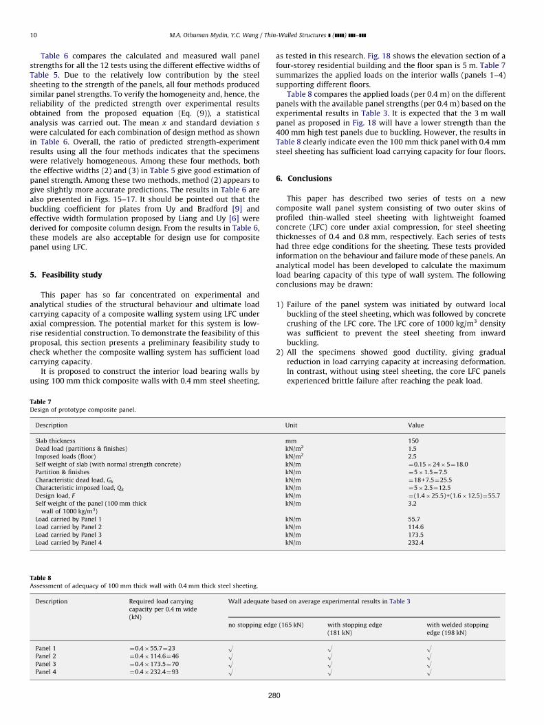
M.A. Othuman Mydin, Y.C. Wang / Thin-Walled Structures ] (]]]]) ]]]–]]]10
Table 6 compares the calculated and measured wall panelstrengths for all the 12 tests using the different effective widths ofTable 5. Due to the relatively low contribution by the steelsheeting to the strength of the panels, all four methods producedsimilar panel strengths. To verify the homogeneity and, hence, thereliability of the predicted strength over experimental resultsobtained from the proposed equation (Eq. (9)), a statisticalanalysis was carried out. The mean x and standard deviation s
were calculated for each combination of design method as shownin Table 6. Overall, the ratio of predicted strength-experimentresults using all the four methods indicates that the specimenswere relatively homogeneous. Among these four methods, boththe effective widths (2) and (3) in Table 5 give good estimation ofpanel strength. Among these two methods, method (2) appears togive slightly more accurate predictions. The results in Table 6 arealso presented in Figs. 15–17. It should be pointed out that thebuckling coefficient for plates from Uy and Bradford [9] andeffective width formulation proposed by Liang and Uy [6] werederived for composite column design. From the results in Table 6,these models are also acceptable for design use for compositepanel using LFC.
5. Feasibility study
This paper has so far concentrated on experimental andanalytical studies of the structural behaviour and ultimate loadcarrying capacity of a composite walling system using LFC underaxial compression. The potential market for this system is low-rise residential construction. To demonstrate the feasibility of thisproposal, this section presents a preliminary feasibility study tocheck whether the composite walling system has sufficient loadcarrying capacity.
It is proposed to construct the interior load bearing walls byusing 100 mm thick composite walls with 0.4 mm steel sheeting,
Table 8Assessment of adequacy of 100 mm thick wall with 0.4 mm thick steel sheeting.
Description Required load carrying
capacity per 0.4 m wide
(kN)
Wall adequate b
no stopping edg
Panel 1 ¼0.4�55.7¼23 OPanel 2 ¼0.4�114.6¼46 OPanel 3 ¼0.4�173.5¼70 OPanel 4 ¼0.4�232.4¼93 O
Table 7Design of prototype composite panel.
Description
Slab thickness
Dead load (partitions & finishes)
Imposed loads (floor)
Self weight of slab (with normal strength concrete)
Partition & finishes
Characteristic dead load, Gk
Characteristic imposed load, Qk
Design load, F
Self weight of the panel (100 mm thick
wall of 1000 kg/m3)
Load carried by Panel 1
Load carried by Panel 2
Load carried by Panel 3
Load carried by Panel 4
28
as tested in this research. Fig. 18 shows the elevation section of afour-storey residential building and the floor span is 5 m. Table 7summarizes the applied loads on the interior walls (panels 1–4)supporting different floors.
Table 8 compares the applied loads (per 0.4 m) on the differentpanels with the available panel strengths (per 0.4 m) based on theexperimental results in Table 3. It is expected that the 3 m wallpanel as proposed in Fig. 18 will have a lower strength than the400 mm high test panels due to buckling. However, the results inTable 8 clearly indicate even the 100 mm thick panel with 0.4 mmsteel sheeting has sufficient load carrying capacity for four floors.
6. Conclusions
This paper has described two series of tests on a newcomposite wall panel system consisting of two outer skins ofprofiled thin-walled steel sheeting with lightweight foamedconcrete (LFC) core under axial compression, for steel sheetingthicknesses of 0.4 and 0.8 mm, respectively. Each series of testshad three edge conditions for the sheeting. These tests providedinformation on the behaviour and failure mode of these panels. Ananalytical model has been developed to calculate the maximumload bearing capacity of this type of wall system. The followingconclusions may be drawn:
1)
ased
e (1
0
Failure of the panel system was initiated by outward localbuckling of the steel sheeting, which was followed by concretecrushing of the LFC core. The LFC core of 1000 kg/m3 densitywas sufficient to prevent the steel sheeting from inwardbuckling.
2)
All the specimens showed good ductility, giving gradualreduction in load carrying capacity at increasing deformation.In contrast, without using steel sheeting, the core LFC panelsexperienced brittle failure after reaching the peak load.on average experimental results in Table 3
65 kN) with stopping edge
(181 kN)
with welded stopping
edge (198 kN)
O OO OO OO O
Unit Value
mm 150
kN/m2 1.5
kN/m2 2.5
kN/m ¼0.15�24�5¼18.0
kN/m ¼5�1.5¼7.5
kN/m ¼18+7.5¼25.5
kN/m ¼5�2.5¼12.5
kN/m ¼(1.4�25.5)+(1.6�12.5)¼55.7
kN/m 3.2
kN/m 55.7
kN/m 114.6
kN/m 173.5
kN/m 232.4

M.A. Othuman Mydin, Y.C. Wang / Thin-Walled Structures ] (]]]]) ]]]–]]] 11
3)
The increase in load carrying capacities of the panels withstopping edge and welded edge can be attributed to the increasedeffective width of the steel sheeting. The load carrying capacities ofpanels with stopping edge and with welded edge were about 10%and 17% higher than those without any stopping edge for bothsteel sheeting thicknesses.4)
The proposed panel strength calculation model takes intoconsideration the effect of profiling on concrete strengthaccording to Wright. This model is able to predict the axialcapacity of the proposed panel very well. To calculate thesteel sheeting effective width, the combination of Uy andBradford plate local buckling coefficients with the Liang andUy effective width formulation appears to give the bestagreement with the experimental results. Nevertheless, thetraditional effective width method proposed by Winter inconjunction with the traditional plate local bucklingcoefficients of Gerard and Becker also gives close resultscompared to the experiments.5)
The proposed panel system, using 100 mm LFC core and0.4 mm steel sheeting, has sufficient load carrying capacity tobe used in low-rise residential construction of 4 floors.Acknowledgements
The first author would like to thank the Ministry of HigherEducation Malaysia and the University of Science Malaysia for
281
their financial support of his PhD study at the University ofManchester. The technical assistance by the laboratory staff at theUniversity of Manchester is greatly appreciated.
References
[1] Md Azree Othuman Mydin, Wang YC. Elevated-temperature thermal proper-ties of lightweight foamed concrete. J Constr Building Mater, in press,doi:10.1016/j.conbuildmat.2010.07.016.
[2] Md Azree Othuman Mydin, Wang YC. Mechanical properties of unstressedlightweight foamed concrete exposed to high temperatures. J Cement ConcrCompos, submitted for publication.
[3] BSI. BS EN 197-1: Cement. Composition, specifications and conformity criteriafor low heat common cements. London: British Standards Institution; 2000.
[4] BSI. BS EN 12620: aggregates for concrete. London: British StandardsInstitution; 2002.
[5] Wright H. The axial load behaviour of composite walling. J Constr Steel Res1998;45:353–75.
[6] Liang QQ, Uy B. Theoretical study on the post-local buckling of steel plates inconcrete-filled box columns. Comput Struct 2000;75:479–90.
[7] Bulson PS. The stability of flat plates. London: Chatto and Windus; 1970.[8] Gerard G, Becker M. Handbook of structural stability: Part I—buckling of flat
plates. NACA TN 1957;3781.[9] Uy B, Bradford MA. Elastic local buckling of steel plates in composite steel–
concrete members. Eng Struct 1996;18:193–200.[10] Winter G. Strength of thin steel compression flanges. Trans ASCE 1947;112:
527–54.


![Lfc 39 - Tristan Yunker Vs Ron Carter [LFC 39]](https://img.pdfslide.us/doc/110x75/55cc7da3bb61ebf4138b4668/lfc-39-tristan-yunker-vs-ron-carter-lfc-39.jpg)