Life insurance mathematics

Abstract: The subject matter and methodology of modern life insurancemathematics are surveyed. Standard insurance products with paymentsdepending only on life history events are described and analyzed in thecommonly used Markov chain model under the assumption of deterministicinterest rates. The actuarial equivalence principle for determining premi-ums and reserves is motivated by risk diversification in large portfolios.Differential equations for reserves and other conditional expected values areobtained and proclaimed basic constructive and computational tools. Thetraditional method for managing non-diversifiable risk arising from changesin e.g. mortality rates and interest rates is outlined; premiums are calcu-lated under prudent assumptions, and systematic surpluses thus created arerepaid as bonus. An alternative way of managing non-diversifiable risk isto link the contractual payments to the development of mortality, interest,and possibly other demographic or economic indexes. Examples of so-calledindex-linked products are given, and premiums and reserves are determinedby combined use of classical actuarial principles and principles of pricingand hedging from financial mathematics. Transfer of non-diversifiable riskto the financial markets through creation of tradeable insurance derivativesis outlined as an idea. Methods for estimation of mortality and other vitalrates, formerly a major issue in life insurance mathematics, are fetched frommodern statistical life history analysis and therefore only briefly described.

Key-words: Life annuity, life assurance, life endowment, life history analysis,time-continuous Markov chain, semi-Markov chain, compound interest, prin-ciple of equivalence, arbitrage pricing theory, with profit contract, surplusand bonus, defined benefits, defined contributions, index linked insurance,securitization.

A. The scope of this survey. Fetching its tools from a number of disci-plines, actuarial science is defined by the direction of its applications ratherthan by the models and methods it makes use of. However, there exists atleast one stream of actuarial science that presents problems and methods suf-ficiently distinct to merit status as an independent area of scientific inquiry– Life insurance mathematics. This is the area of applied mathematics thatstudies risk associated with life and pension insurance and methods for man-agement of such risk. Under this strict definition, its models and methodsare described as they present themselves today, sustained by contemporary

1

mathematics, statistics, and computation technology. No attempt is madeto survey its two millenniums of past history, its vast collection of techniquesthat were needed before the advent of scientific computation, or the count-less details that arise from its practical implementation to a wide range ofproducts in a strictly regulated industry.

B. Basic notions of payments and interest. In the general contextof financial services, consider a financial contract between a company anda customer. The terms and conditions of the contract generate a streamof payments, benefits from the company to the customer less contributionsfrom the customer to the company. They are represented by a paymentfunction

B(t) = total amount paid in the time interval [0,t] ,

t ≥ 0, time being reckoned from the inception of the policy. This func-tion is taken to be right-continuous, B(t) = limτ↘t B(τ), with existing left-limits, B(t−) = limτ↗t B(τ). When different from 0, the jump ∆B(t) =B(t)−B(t−) represents a lump sum payment at time t. There may also bepayments due continuously at rate b(t) per time unit at any time t. Thus,the payments made in any small time interval [t, t + dt) total

dB(t) = b(t) dt + ∆B(t) .

Payments are currently invested (contributions deposited and benefitswithdrawn) into an account that bears interest at rate r(t) at time t. Thebalance of the company’s account at time t, called the retrospective reserve,is the sum of all past and present payments accumulated with interest,

U(t) =∫ t

0−e∫ t

τ r(s) dsd(−B)(τ) ,

where∫ t0− =

∫[0, t]. Upon differentiating this relationship, one obtains the

dynamics

dU(t) = U(t) r(t) dt− dB(t) , (1)

showing how the balance increases with interest earned on the current re-serve and net payments into the account.

The company’s discounted (strictly) future net liability at time t is

V(t) =∫ n

te−

∫ τt r(s) dsdB(τ) . (2)

2

Its dynamics,dV(t) = V(t) r(t) dt− dB(t) ,

shows how the debt increases with interest and decreases with net redemp-tion.

C. Valuation of financial contracts. At any time t the company has toprovide a prospective reserve V (t) that adequately meets its future obliga-tions under the contract. If the future payments and interest rates would beknown at time t (e.g. a fixed plan savings account in an economy with fixedinterest), then so would the present value in (2), and an adequate reservewould be V (t) = V(t). For the contract to be economically feasible, no partyshould profit at the expense of the other, so the value of the contributionsmust be equal to the value of the benefits at the outset:

∆B(0) + V (0) = 0 . (3)

If future payments and interest rates are uncertain so that V(t) is un-known at time t, then reserving must involve some principles beyond thoseof mere accounting. A clear-cut case is when the payments are derivatives(functions) of certain assets (securities), one of which is a money accountwith interest rate r. Principles for valuation of such contracts are deliv-ered by modern financial mathematics, see e.g. [3]. We will describe thembriefly in lay terms. Suppose there is a finite number of basic assets thatcan be traded freely, in unlimited positive or negative amounts (taking longor short positions) and without transaction costs. An investment portfoliois given by the number of shares held in each asset at any time. The sizeand the composition of the portfolio may be dynamically changed throughsales and purchases of shares. The portfolio is said to be self-financing if,after its initiation, every purchase of shares in some assets is fully financedby selling shares in some other assets (the portfolio is currently rebalanced,with no further infusion or withdrawal of capital). A self-financing portfoliois an arbitrage if the initial investment is negative (the investor borrows themoney) and the value of the portfolio at some later time is non-negativewith probability one. A fundamental requirement for a market to be well-functioning is that it does not admit arbitrage opportunities. A financialclaim that depends entirely on the prices of the basic securities is called a fi-nancial derivative. Such a claim is said to be attainable if it can be perfectlyreproduced by a self-financing portfolio. The no arbitrage regime dictatesthat the price of a financial derivative must at any time be the current value

3

of the self-financing portfolio that reproduces it. It turns out that the priceat time t of a stream of attainable derivative payments B is of the form

V (t) = E [V(t)| Gt] , (4)

where E is the expected value under a so-called equivalent martingale mea-sure derived from the price processes of the basic assets, and Gt representall market events observed up to and including time t. Again, the contractmust satisfy (3), which determines the initial investment −∆B(0) neededto buy the self-financing portfolio. The financial market is complete if everyfinancial derivative is attainable. If the market is not complete, there is nounique price for every derivative, but any pricing principle obeying the noarbitrage requirement must be of the form (4).

D. Valuation of life insurance contracts by the principle of equiv-alence. Characteristic features of life insurance contracts are, firstly, thatthe payments are contingent on uncertain individual life history events(largely unrelated to market events) and, secondly, that the contracts arelong term and binding to the insurer. Therefore, there exists no liquid mar-ket for such contracts and they can not be valued by the mere principles ofaccounting and finance described above. Pricing of life insurance contractsand management of the risk associated with them are the paramount issuesof life insurance mathematics.

The paradigm of traditional life insurance is the so-called principle ofequivalence, which is based on the notion of risk diversification in a largeportfolio under the assumption that the future development of interest ratesand other relevant economic and demographic conditions are known. Con-sider a portfolio of m contracts currently in force. Switching to calendartime, denote the payment function of contract No i by Bi and denote itsdiscounted future net liabilities at time t by V i(t) =

∫ nt e−

∫ τt r(s) dsdBi(τ).

Let Ht represent the life history by time t (all individual life history eventsobserved up to and including time t) and introduce ξi = E[V i(t)|Ht], σ2

i =Var[V i(t)|Ht], and s2

m =∑m

i=1 σ2i . Assume that the contracts are indepen-

dent and that the portfolio grows in a balanced manner such that s2m goes

to infinity without being dominated by any single term σ2i . Then, by the

central limit theorem, the standardized sum of total discounted liabilitiesconverges in law to the standard normal distribution as the size of the port-folio increases: ∑m

i=1(V i(t)− ξi)sm

L→ N(0, 1) . (5)

4

Suppose the company provides individual reserves given by

V i(t) = ξi + ε σ2i (6)

for some ε > 0. Then

P

[m∑

i=1

V i(t)−m∑

i=1

V i(t) > 0

∣∣∣∣∣Ht

]= P

[ ∑mi=1(V i(t)− ξi)

sm< ε sm

∣∣∣∣Ht

],

and it follows from (5) that the total reserve covers the discounted liabilitieswith a (conditional) probability that tends to 1. Similarly, taking ε < 0in (6), the total reserve covers discounted liabilities with a probability thattends to 0. The benchmark value ε = 0 defines the actuarial principle ofequivalence, which for an individual contract reads (drop topscript i):

V (t) = E[∫ n

te−

∫ τt r(s) dsdB(τ)

∣∣∣∣Ht

]. (7)

In particular, for given benefits the premiums should be designed so as tosatisfy (3).

E. Life and pension insurance products. Consider a life insurancepolicy issued at time 0 for a finite term of n years. There is a finite setof possible states of the policy, Z = {0, 1, . . . , J}, 0 being the initial state.Denote the state of the policy at time t by Z(t). The uncertain course ofpolicy is modeled by taking Z to be a stochastic process. Regarded as afunction from [0, n] to Z, Z is assumed to be right-continuous, with a finitenumber of jumps, and commencing from Z(0) = 0. We associate with theprocess Z the indicator processes Ig and counting processes Ngh defined,respectively, by Ig(t) = 1[Z(t) = g] (1 or 0 according as the policy is in thestate g or not at time t) and Ngh(t) = ]{τ ; Z(τ−) = g, Z(τ) = h, τ ∈ (0, t]}(the number of transitions from state g to state h (h 6= g) during the timeinterval (0, t]).

The payments B generated by an insurance policy are typically of theform

dB(t) =∑

g

Ig(t) dBg(t) +∑g 6=h

bgh(t) dNgh(t) , (8)

where each Bg is a payment function specifying payments due during so-journs in state g (a general life annuity), and each bgh specifying lump sum

5

payments due upon transitions from state g to state h (a general life as-surance). When different from 0, ∆Bg(t) represents a lump sum (generallife endowment) payable in state g at time t. Positive amounts representbenefits and negative amounts represent premiums. In practice premiumsare only of annuity type.

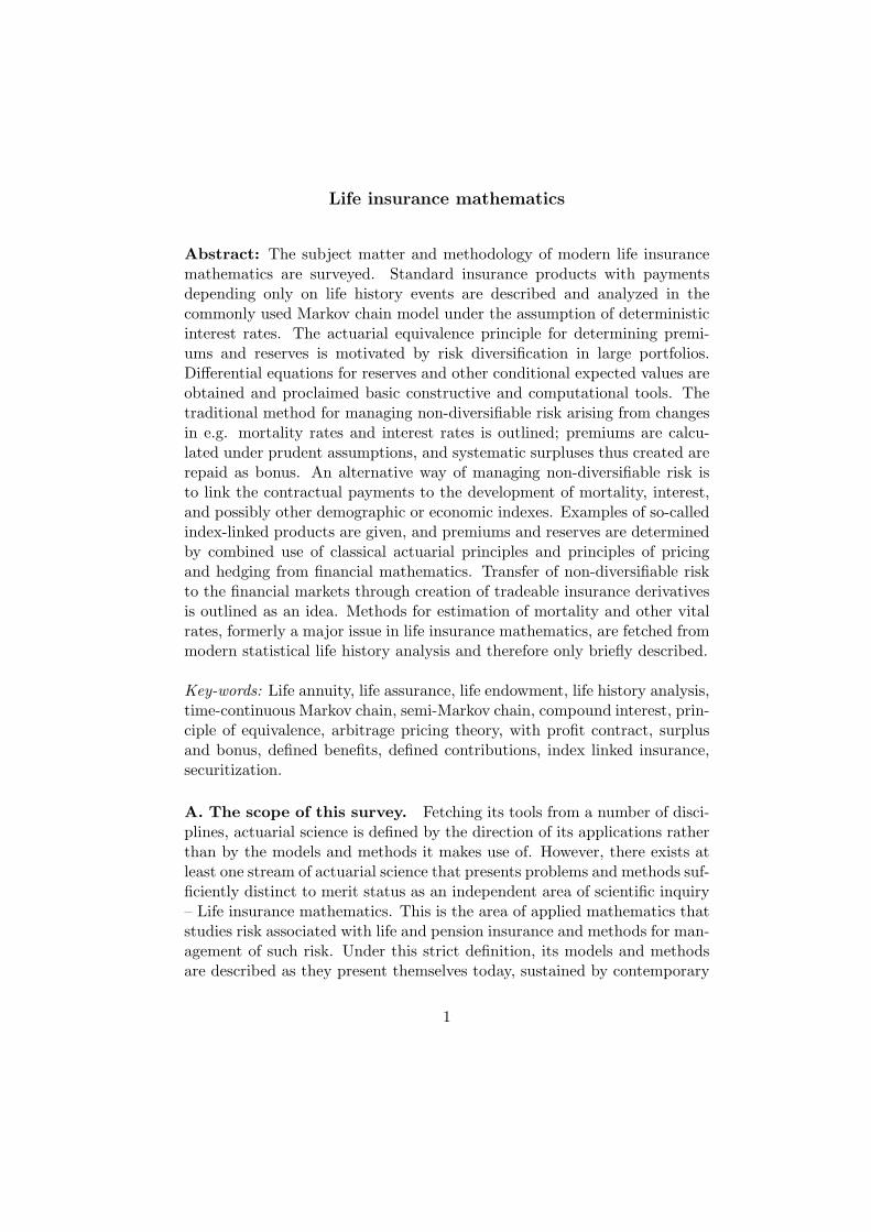
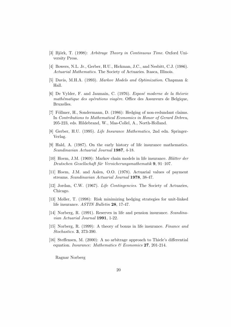
Figure 1 shows a flow-chart for a policy on a single life with paymentsdependent only on survival and death. We list the basic forms of benefits: Ann-year term insurance with sum insured 1 payable immediately upon death,b01(t) = 1[t ∈ (0, n)]; An n-year life endowment with sum 1, ∆B0(n) = 1;An n-year life annuity payable annually in arrears, ∆B0(t) = 1, t = 1, . . . , n;An n-year life annuity payable continuously at rate 1 per year, b0(t) = 1[t ∈(0, n)]; An (n − m)-year annuity deferred in m years payable continuouslyat rate 1 per year, b0(t) = 1[t ∈ (m,n)]. Thus, an n-year term insurancewith sum insured b against premium payable continuously at rate c per yearis given by dB(t) = b dN01(t) − c I0(t) dt for 0 ≤ t < n and dB(t) = 0 fort ≥ n.

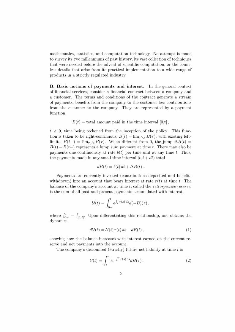
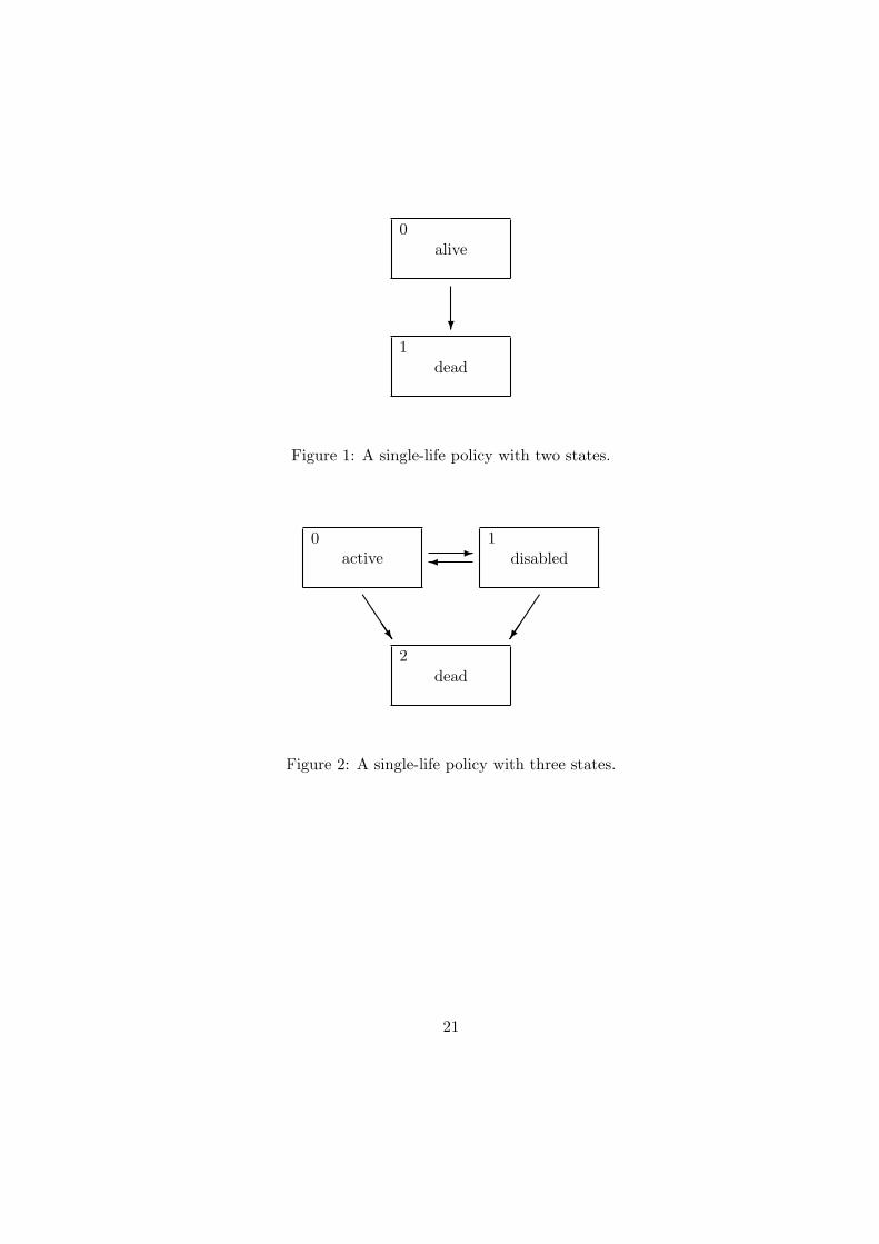
The flow-chart in Figure 2 is apt to describe a single-life policy with pay-ments that may depend on the state of health of the insured. For instance,an n-year endowment insurance (a combined term insurance and and life en-dowment) with sum insured b, against premium payable continuously at ratec while active (waiver of premium during disability), is given by dB(t) =b (dN02(t) + dN12(t)) − c I0(t) dt, 0 ≤ t < n, dB(n) = b (I0(n) + I1(n)),dB(t) = 0 for t > n.

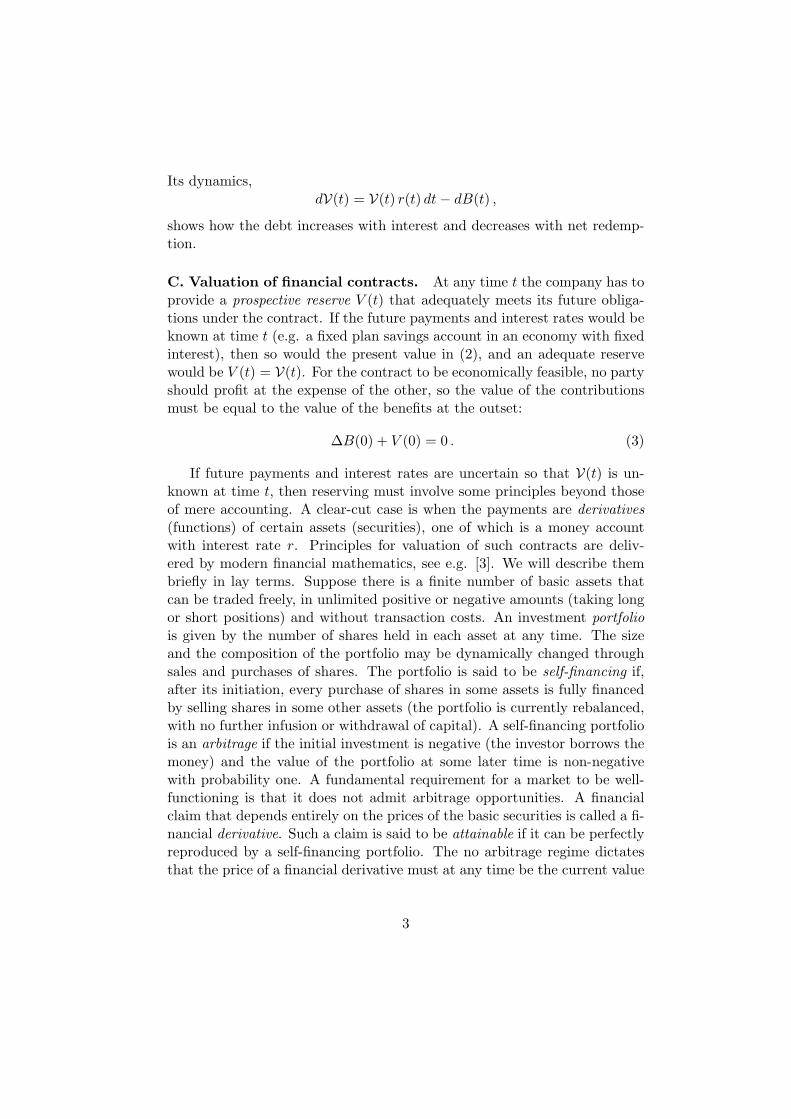
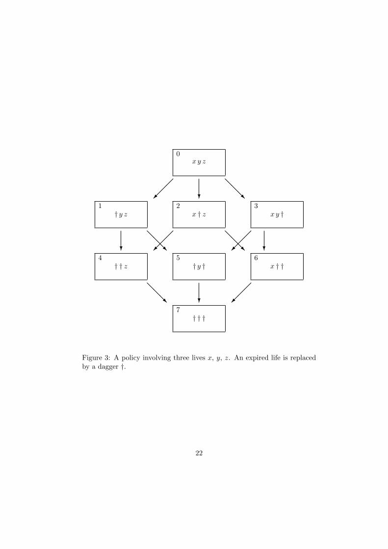
The flow-chart in Figure 3 is apt to describe a multi-life policy involvingthree lives called x, y, and z. For instance, an n-year insurance with sum bpayable upon the death of the last survivor against premium payable as longas all three are alive is given by dB(t) = b (dN47(t) + dN57(t) + dN67(t)) −c I0(t) dt, 0 ≤ t < n, dB(t) = 0 for t ≥ n.

F. The Markov chain model for the policy history. The break-through of stochastic processes in life insurance mathematics was markedby Hoem’s 1969 paper [10], where the process Z was modeled as a time-continuous Markov chain. The Markov property means that the futurecourse of the process is independent of its past if the present state is known:For 0 < t1 < · · · < tq and j1, . . . , jq in Z,

P[Z(tq) = jq |Z(tp) = jp , p = 1, . . . , q − 1] = P[Z(tq) = jq |Z(tq−1) = jq−1] .

It follows that the simple transition probabilities,

pgh(t, u) = P[Z(u) = h |Z(t) = g] ,

6

determine the finite-dimensional marginal distributions through

P[Z(tp) = jp , p = 1, . . . , q] = p0j1(0, t1) pj1j2(t1, t2) · · · pjq−1jq(tq−1, tq) ,

hence they also determine the entire probability law of the process Z. It ismoreover assumed that, for each pair of states g 6= h and each time t, thelimit

µgh(t) = limu↘t

pgh(t, u)u− t

,

exists. It is called the intensity of transition from state g to state h at timet. In other words,

pgh(t, u) = µgh(t) dt + o(dt) ,

where o(dt) denotes a term such that o(dt)/dt → 0 as dt → 0. The inten-sities, being one-dimensional and easy to interpret as “instantaneous con-ditional probabilities of transition per time unit”, are the basic entities inthe probability model. They determine the simple transition probabilitiesuniquely as solutions to sets of differential equations. The Kolmogorov back-ward differential equations for the pjg(t, u), seen as functions of t ∈ [0, u] forfixed g and u, are

∂

∂tpjg(t, u) = −

∑k;k 6=j

µjk(t) (pkg(t, u)− pjg(t, u)) , (9)

with side conditions pgg(u, u) = 1 and pjg(u, u) = 0 for j 6= g. The Kol-mogorov forward equations for the pgj(s, t), seen as functions of t ∈ [s, n] forfixed g and s, are

∂

∂tpgj(s, t) =

∑i;i6=j

pgi(s, t)µij(t) dt − pgj(s, t)µj·(t) dt , (10)

with obvious side conditions at t = s. The forward equations are some-times the more convenient because, for any fixed t, the functions pgj(s, t),j = 0, . . . , J , are probabilities of disjoint events and therefore sum to 1. Atechnique for obtaining such differential equations is sketched in ParagraphG.

A differential equation for the sojourn probability,

pgg(t, u) = P[Z(τ) = g , τ ∈ (t, u] |Z(t) = g] ,

is easily put up and solved to give

pgg(t, u) = e−∫ u

t µg ·(s) ds ,

7

where µg ·(t) =∑

h, h6=g µgh(t) is the total intensity of transition out of stateg at time t.

To see that the intensities govern the probability law of the process Z,consider a fully specified path of Z, starting form the initial state g0 = 0 attime t0 = 0, sojourning there until time t1, making a transition from g0 tog1 in [t1, t1 + dt1), sojourning there until time t2, making a transition fromg1 to g2 in [t2, t2 +dt2), and so on until making its final transition from gq−2

to gq−1 in [tq−1, tq−1 + dtq−1), and sojourning there until time tq = n. Theprobability of this elementary event is a product of sojourn probabilities andinfinitesimal transition probabilities, hence a function only of the intensities:

e−

∫ t1t0

µg0 ·(s) dsµg0g1(t1) dt1 e−

∫ t2t1

µg1 ·(s) ds µg1g2(t2) dt2 · · · e−

∫ tqtq−1

µgq−1·(s) ds

= e∑q−1

p=1 ln µgp−1gp (tp)−∑q

p=1

∑h;h6=gp−1

∫ tptp−1

µgp−1h(s) dsdt1 . . . dtq−1 . (11)

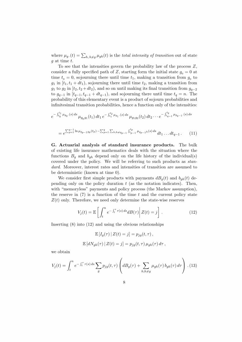
G. Actuarial analysis of standard insurance products. The bulkof existing life insurance mathematics deals with the situation where thefunctions Bg and bgh depend only on the life history of the individual(s)covered under the policy. We will be referring to such products as stan-dard. Moreover, interest rates and intensities of transition are assumed tobe deterministic (known at time 0).

We consider first simple products with payments dBg(t) and bgh(t) de-pending only on the policy duration t (as the notation indicates). Then,with “memoryless” payments and policy process (the Markov assumption),the reserve in (7) is a function of the time t and the current policy stateZ(t) only. Therefore, we need only determine the state-wise reserves

Vj(t) = E[∫ n

te−

∫ τt r(s) dsdB(τ)

∣∣∣∣ Z(t) = j

]. (12)

Inserting (8) into (12) and using the obvious relationships

E [Ig(τ) |Z(t) = j] = pjg(t, τ) ,

E [dNgh(τ) |Z(t) = j] = pjg(t, τ) µgh(τ) dτ ,

we obtain

Vj(t) =∫ n

te−

∫ τt r(s) ds

∑g

pjg(t, τ)

dBg(τ) +∑

h;h 6=g

µgh(τ) bgh(τ) dτ

. (13)

8

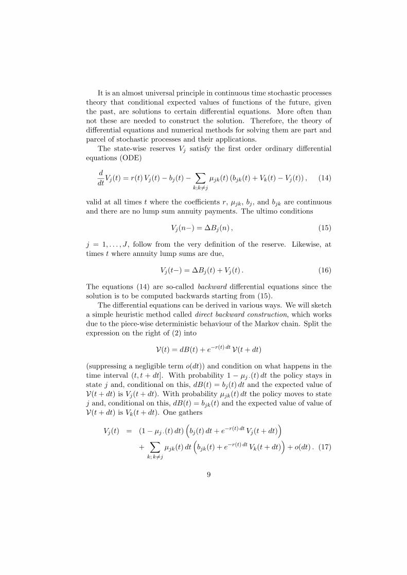
It is an almost universal principle in continuous time stochastic processestheory that conditional expected values of functions of the future, giventhe past, are solutions to certain differential equations. More often thannot these are needed to construct the solution. Therefore, the theory ofdifferential equations and numerical methods for solving them are part andparcel of stochastic processes and their applications.

The state-wise reserves Vj satisfy the first order ordinary differentialequations (ODE)

d

dtVj(t) = r(t) Vj(t)− bj(t)−

∑k;k 6=j

µjk(t) (bjk(t) + Vk(t)− Vj(t)) , (14)

valid at all times t where the coefficients r, µjk, bj , and bjk are continuousand there are no lump sum annuity payments. The ultimo conditions

Vj(n−) = ∆Bj(n) , (15)

j = 1, . . . , J , follow from the very definition of the reserve. Likewise, attimes t where annuity lump sums are due,

Vj(t−) = ∆Bj(t) + Vj(t) . (16)

The equations (14) are so-called backward differential equations since thesolution is to be computed backwards starting from (15).

The differential equations can be derived in various ways. We will sketcha simple heuristic method called direct backward construction, which worksdue to the piece-wise deterministic behaviour of the Markov chain. Split theexpression on the right of (2) into

V(t) = dB(t) + e−r(t) dt V(t + dt)

(suppressing a negligible term o(dt)) and condition on what happens in thetime interval (t, t + dt]. With probability 1 − µj ·(t) dt the policy stays instate j and, conditional on this, dB(t) = bj(t) dt and the expected value ofV(t + dt) is Vj(t + dt). With probability µjk(t) dt the policy moves to statej and, conditional on this, dB(t) = bjk(t) and the expected value of value ofV(t + dt) is Vk(t + dt). One gathers

Vj(t) = (1− µj ·(t) dt)(bj(t) dt + e−r(t) dt Vj(t + dt)

)+

∑k; k 6=j

µjk(t) dt(bjk(t) + e−r(t) dt Vk(t + dt)

)+ o(dt) . (17)

9

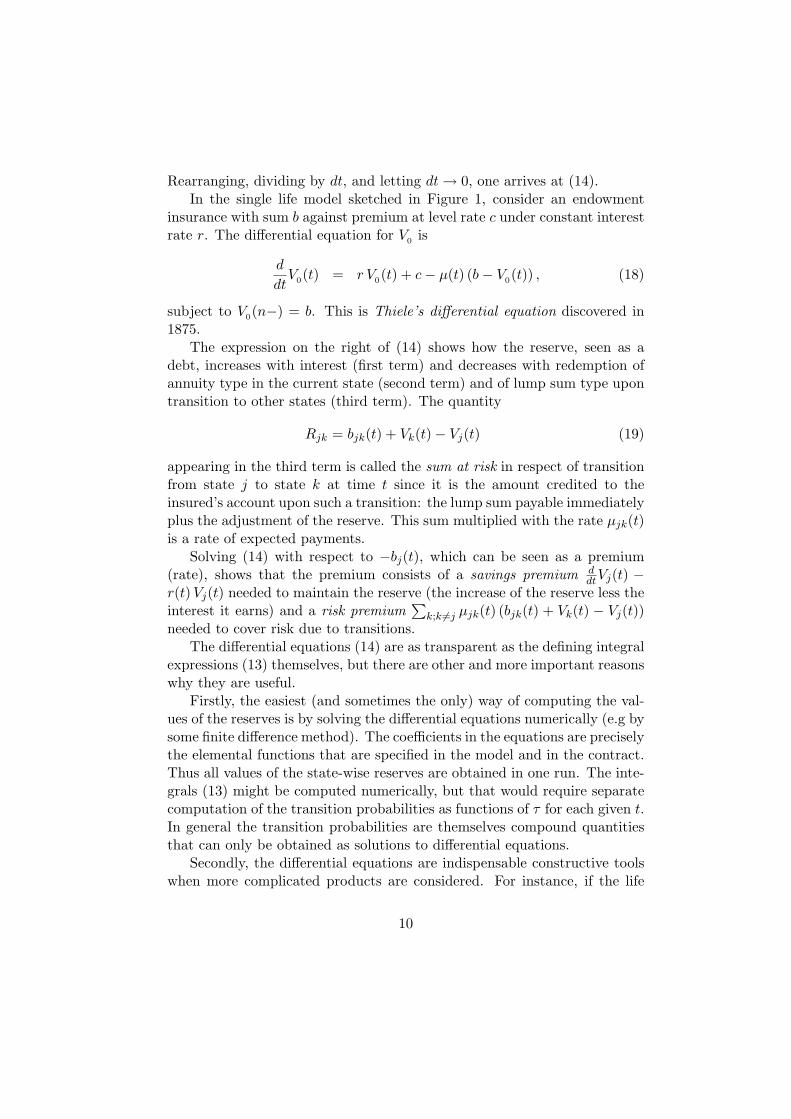
Rearranging, dividing by dt, and letting dt → 0, one arrives at (14).In the single life model sketched in Figure 1, consider an endowment

insurance with sum b against premium at level rate c under constant interestrate r. The differential equation for V0 is

d

dtV0(t) = r V0(t) + c− µ(t) (b− V0(t)) , (18)

subject to V0(n−) = b. This is Thiele’s differential equation discovered in1875.

The expression on the right of (14) shows how the reserve, seen as adebt, increases with interest (first term) and decreases with redemption ofannuity type in the current state (second term) and of lump sum type upontransition to other states (third term). The quantity

Rjk = bjk(t) + Vk(t)− Vj(t) (19)

appearing in the third term is called the sum at risk in respect of transitionfrom state j to state k at time t since it is the amount credited to theinsured’s account upon such a transition: the lump sum payable immediatelyplus the adjustment of the reserve. This sum multiplied with the rate µjk(t)is a rate of expected payments.

Solving (14) with respect to −bj(t), which can be seen as a premium(rate), shows that the premium consists of a savings premium d

dtVj(t) −r(t) Vj(t) needed to maintain the reserve (the increase of the reserve less theinterest it earns) and a risk premium

∑k;k 6=j µjk(t) (bjk(t) + Vk(t) − Vj(t))

needed to cover risk due to transitions.The differential equations (14) are as transparent as the defining integral

expressions (13) themselves, but there are other and more important reasonswhy they are useful.

Firstly, the easiest (and sometimes the only) way of computing the val-ues of the reserves is by solving the differential equations numerically (e.g bysome finite difference method). The coefficients in the equations are preciselythe elemental functions that are specified in the model and in the contract.Thus all values of the state-wise reserves are obtained in one run. The inte-grals (13) might be computed numerically, but that would require separatecomputation of the transition probabilities as functions of τ for each given t.In general the transition probabilities are themselves compound quantitiesthat can only be obtained as solutions to differential equations.

Secondly, the differential equations are indispensable constructive toolswhen more complicated products are considered. For instance, if the life

10

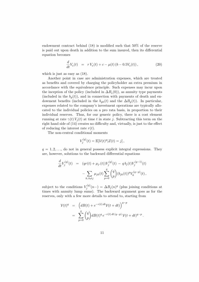
endowment contract behind (18) is modified such that 50% of the reserveis paid out upon death in addition to the sum insured, then its differentialequation becomes

d

dtV0(t) = r V0(t) + c− µ(t) (b− 0.5V0(t)) , (20)

which is just as easy as (18).Another point in case are administration expenses, which are treated

as benefits and covered by charging the policyholder an extra premium inaccordance with the equivalence principle. Such expenses may incur uponthe inception of the policy (included in ∆B0(0)), as annuity type payments(included in the bg(t)), and in connection with payments of death and en-dowment benefits (included in the bgh(t) and the ∆Bg(t)). In particular,expenses related to the company’s investment operations are typically allo-cated to the individual policies on a pro rata basis, in proportion to theirindividual reserves. Thus, for our generic policy, there is a cost elementrunning at rate γ(t) Vj(t) at time t in state j. Subtracting this term on theright hand side of (14) creates no difficulty and, virtually, is just to the effectof reducing the interest rate r(t).

The non-central conditional moments

V(q)j (t) = E[V(t)q|Z(t) = j] ,

q = 1, 2, . . ., do not in general possess explicit integral expressions. Theyare, however, solutions to the backward differential equations

d

dtV

(q)j (t) = (qr(t) + µj·(t))V

(q)j (t) − q bj(t)V

(q−1)j (t)

−∑

k; k 6=j

µjk(t)q∑

p=0

(q

p

)(bjk(t))pV

(q−p)k (t) ,

subject to the conditions V(q)j (n−) = ∆Bj(n)q (plus joining conditions at

times with annuity lump sums). The backward argument goes as for thereserves, only with a few more details to attend to, starting from

V(t)q =(dB(t) + e−r(t) dtV(t + dt)

)q−p

=q∑

p=0

(q

p

)dB(t)q e−r(t) dt (q−p) V(t + dt)q−p .

11

Higher order moments shed light on the risk associated with the portfolio.Recalling (5) and using the notation in Paragraph D, a solvency marginapproximately equal to the upper ε-fractile in the distribution of the dis-counted outstanding net liability is given by

∑mi=1 ξi + c1−εsm, where c1−ε

is the upper ε-fractile of the standard normal distribution. More refinedestimates of the fractiles of the total liability can be obtained by involvingthree or more moments.

H. Path-dependent payments and semi-Markov models. The tech-nical matters in Paragraphs F-G become more involved if the contractualpayments or the transition intensities depend on the past life history. Wewill consider examples where they may depend on the sojourn time S(t) thathas elapsed since entry into the current state, henceforth called the state du-ration. Thus, if Z(t) = j and S(t−) = s at policy duration t, the transitionintensities and payments are of the form µjk(s, t), bj(s, t), and bjk(s, t). Toease exposition, we disregard intermediate lump sum annuities, but allow ofterminal endowments ∆Bj(s, n) at time n. The state-wise reserve will nowbe a function of the form Vj(s, t).

In simple situations (e.g. no possibility of return to previously visitedstates) one may still work out integral expressions for probabilities and re-serves (they will be multiple integrals). The differential equation approachalways works, however. The relationship (17) modifies to

Vj(s, t) = (1− µj · (s, t) dt)(bj(s, t) dt + e−r(t) dtVj(s + dt, t + dt)

)+

∑k; k 6=j

µjk(s, t) dt (bjk(s, t) + Vk(0, t)) + o(dt) ,

from which one obtains the first order partial differential equations

∂

∂tVj(s, t) = r(t)Vj(s, t)−

∂

∂sVj(s, t)− bj(s, t)

−∑

k;k 6=j

µjk(s, t) (bjk(s, t) + Vk(0, t)− Vj(s, t)) , (21)

subject to the conditions

Vj(s, n−) = ∆Bj(s, n) . (22)

We give two examples of payments dependent on state duration. In theframework of the disability model in Figure 2, an n-year disability annuitypayable at rate 1 only after a qualifying period of q, is given by b1(s, t) =

12

1[q < s < t < n]. In the framework of the three-lives model sketched inFigure 3, an n-year term insurance of 1 payable upon the death of y if zis still alive and x is dead and has been so for at least q years, is given byb14(s, t) = 1[q < s < t < n].

Probability models with intensities dependent on state duration areknown as a semi-Markov models. A case of support to their relevance isthe disability model in Figure 2. If there are various forms of disability,then the state duration may carry information about the severity of thedisability and hence about prospects of longevity and recovery.

I. Managing non-diversifiable risk for standard insurance prod-ucts. Life insurance policies are typically long term contracts, with timehorizons wide enough to see substantial variations in interest, mortality, andother economic and demographic conditions affecting the economic result ofthe portfolio. The rigid conditions of the standard contract leave no roomfor the insurer to meet adverse developments of such conditions; he can notcancel contracts that are in force and also not reduce their benefits or raisetheir premiums. Therefore, with standard insurance products there is asso-ciated a risk that cannot be diversified by increasing the size of the portfolioas in Paragraph D. The limit operation leading to (7) was made under theassumption of fixed interest. In an extended set-up, with random economicand demographic factors, this amounts to conditioning on Gn, the economicand demographic development over the term of the contract. Instead of (7),one gets

V (t) = E[∫ n

te−

∫ τt r(s) dsdB(τ)

∣∣∣∣Ht, Gn

]. (23)

At time t only Gt is known, so (23) is not a feasible reserve. In particular,the equivalence principle (3), recast as

∆B0(0) + E[∫ n

0e−

∫ τ0 r(s) dsdB(τ)

∣∣∣∣Gn

]= 0 , (24)

is also infeasible since benefits and premiums are fixed at time 0 when Gn

cannot be anticipated.The traditional way of managing the non-diversifiable risk is to charge

premiums sufficiently high to cover, on the average in the portfolio, thecontractual benefits under all likely economic-demographic scenarios. Thesystematic surpluses that (most likely) will be generated by such prudentlycalculated premiums belong to the insured and are paid back in arrears as

13

the history Gt unfolds. Such contracts are called participating policies orwith-profit contracts.

The repayments, called dividends or bonus, are represented by a paymentfunction D. They should be controlled in such a manner as to ultimatelyrestore equivalence when the full history is known at time n:

∆B0(0) + E[∫ n

0e−

∫ τ0 r(s) ds(dB(τ) + dD(τ))

∣∣∣∣Gn

]= 0 , (25)

A common way of designing the prudent premium plan is, in the frame-work of Paragraphs D-H, to calculate premiums and reserves on a so-calledtechnical basis with interest rate r∗ and transition intensities µ∗jk that repre-sent a worst-case-scenario. Equipping all technical quantities with an aster-isk, we denote the corresponding reserves by V ∗

j , the sums at risk by R∗jk etc.

The surplus generated by time t is, quite naturally, defined as the excess ofthe factual retrospective reserve over the contractual prospective reserve,

S(t) = U(t)−J∑

j=0

Ij V ∗j (t) . (26)

Upon differentiating this expression, using (1), (8), (14), and the obviousrelationship dIj(t) =

∑k; k 6=j(dNkj(t) − dNjk(t)), one obtains after some

rearrangement that

dS(t) = S(t) r(t) dt + dC(t) + dM(t) , (27)

where

dC(t) =J∑

j=0

Ij(t) cj(t) dt , (28)

cj(t) = (r(t)− r∗) V ∗j (t) +

∑k; k 6=j

R∗jk(t)(µ

∗jk(t)− µjk(t)) , (29)

dM(t) = −∑j 6=k

R∗jk(dNjk(t)− Ij(t) µjk(t) dt) . (30)

The right hand side of (27) displays the dynamics of the surplus. The firstterm is the interest earned on the current surplus. The last term, givenby (30), is purely erratic and represents the policy’s instantaneous random

14

deviation from the expected development. The second term, given by (28),is the systematic contribution to surplus, and (29) shows how it decom-poses into gains due to prudent assumptions about interest and transitionintensities in each state.

One may show that (25) is equivalent to

E[∫ n

0e−

∫ τ0 r(s) ds(dC(τ)− dD(τ))

∣∣∣∣Gn

]= 0 , (31)

which says that, on the average over the portfolio, all surpluses are to berepaid as dividends.

The dividend payments D are controlled by the insurer. Since negativedividends are not allowed, it is possible that (31) cannot be ultimately at-tained if the contributions to surplus turn negative (the technical basis wasnot sufficiently prudent) and/or dividends were paid out prematurely. De-signing the dividend plan D is therefore a major issue, and it can be seenas a problem in optimal stochastic control theory. For a general account ofthe point process version of this theory, see [5]. Various schemes used inpractice are described in [15]. The simplest (and least cautious one) is theso-called contribution plan, whereby surpluses are repaid currently as theyarise: D = C.

The much discussed issue of guaranteed interest takes a clear form in theframework of the present theory. Focusing on interest, suppose the technicalintensities µ∗jk are the same as the factual µjk so that the surplus emergesonly from the excess of the factual interest rate r(t) over the technical rater∗:

dC(t) = (r(t)− r∗) V ∗Z(t)(t) dt .

Under the contribution plan dD(t) must be set to 0 if dC(t) < 0, and theinsurer will therefore have to cover the negative contributions dC−(t) = (r∗−r(t))+ V ∗

Z(t)(t) dt. Averaging out the life history randomness, the discountedvalue of these claims is∫ n

0e−

∫ τ0 r(s) ds(r∗ − r(τ))+

J∑j=0

p0j(0, τ) V ∗j (τ) dτ . (32)

Mobilizing the principles of arbitrage pricing theory set out in ParagraphC, we conclude that the interest guarantee inherent in the present schemehas a market price which is the expected value of (32) under the equivalentmartingale measure. Charging a down premium equal to this price at time 0would eliminate the downside risk of the contribution plan without violatingthe format of the with-profit scheme.

15

J. Unit-linked insurance. The dividends D redistributed to holders ofstandard with-profit contracts can be seen as a way of adapting the benefitspayments to the development of the non-diversifiable risk factors of Gt, 0 <t ≤ n. Alternatively one could specify in the very terms of the contractthat the payments will depend, not only on life history events, but alsoon the development of interest, mortality, and other economic-demographicconditions. One such approach is the unit-linked contract, which relates thebenefits to the performance of the insurer’s investment portfolio. To keepthings simple, let the interest rate r(t) be the only uncertain non-diversifiablefactor. A straightforward way of eliminating the interest rate risk is to letthe payment function under the contract be of the form

dB(t) = e∫ t0 r(s) ds dB0(t) , (33)

where B0 is a baseline payment function dependent only on the life history.This means that all payments, premiums and benefits, are index-regulatedwith the value of a unit of the investment portfolio. Inserting this into (24),assuming that life history events and market events are independent, theequivalence requirement becomes

∆B00(0) + E

[∫ n

0dB0(τ)

]= 0 .

This requirement does not involve the future interest rates and can be metby setting an equivalence baseline premium level at time 0.

Perfect unit-linked products of the form (33) are not offered in prac-tice. Typically, only the sum insured (of e.g. a term insurance or a lifeendowment) is index-regulated while the premiums are not. Moreover, thecontract usually comes with a guarantee that the sum insured will not beless than a certain nominal amount. Averaging out over the life histories,the payments become purely financial derivatives, and pricing goes by theprinciples described in Paragraph C. If random life history events are keptpart of the model, one faces a pricing problem in an incomplete market.This problem was formulated and solved in [13] in the framework of thetheory of risk minimization [7].

K. Defined benefits and defined contributions. With-profit and unit-linked are two just two ways of adapting benefits to the long-term devel-opment of non-diversifiable risk factors. The former does not include theadaptation rule in the terms of the contract, whereas the latter does. We

16

mention two other arch-type insurance schemes that are widely used in prac-tice. Defined benefits means literally that only the benefits are specified inthe contract, either in nominal figures as in the with-profit contract or inunits of some index. A commonly used index is the salary (final or average)of the insured. In that case also the contributions (premiums) are usuallylinked to the salary (typically a certain percentage of the annual income).Risk management of such a scheme is a matter of designing the rule for col-lection of contributions. Unless the future benefits can be precisely predictedor reproduced by dynamic investment portfolios, defined benefits leave theinsurer with a major non-diversifiable risk. Defined benefits are graduallybeing replaced with their opposite, defined contributions, with only premi-ums specified in the contract. This scheme has much in common with thetraditional with-profit scheme, but leaves more flexibility to the insurer asbenefits do not come with a minimum guarantee.

L. Securitization. Generally speaking, and recalling Paragraph C, anyintroduction of new securities in a market helps to complete it. Securitiza-tion means creating tradeable securities that may serve to make non-tradedclaims attainable. This device, well known and widely used in the com-modities markets, was introduced in non-life insurance in the 1990-es whenexchanges and insurance corporations launched various forms of insurancederivatives aimed to transfer catastrophe risk to the financial markets. Se-curitization of non-diversifiable risk in life insurance, e.g. through bondswith coupons related to mortality experience, is conceivable. If successful,it would open new opportunities of financial management of life insurancerisk by the principles described in Paragraph C. A work in this spirit is [16],where market attitudes are modeled for all forms of risk associated with alife insurance portfolio, leading to market values for reserves.

M. Statistical inference. The theory of inference in point process modelsis a well developed area of statistical science, see e.g. [1]. We will justindicate how it applies to the Markov chain model and only consider theparametric case where the intensities are of the form µgh(t; θ) with θ somefinite-dimensional parameter.

The likelihood function for an individual policy is obtained upon in-serting the observed policy history (the processes Ig and Ngh) in (11) and

17

dropping the dti:

Λ = exp

∑g 6=h

∫(lnµgh(τ)dNgh(τ)− µgh(τ)Ig(τ)dτ)

. (34)

The integral ranges over the period of observation. In this context the timeparameter t will typically be the age of the insured.

The total likelihood for the observations from a portfolio of m indepen-dent risk is the product of the individual likelihoods and, therefore, of thesame form as (34), with Ig and Ngh replaced by

∑mi=1 Ii

g and∑m

i=1 N igh. The

maximum likelihood estimator θ of the parameter vector θ is obtained asthe solution to the likelihood equations

∂

∂θlnΛ

∣∣∣∣θ=θ

= 0 .

Under regularity conditions, θ is asymptotically normally distributed withmean θ and a variance matrix that is the inverse of the information matrix

Eθ

(− ∂2

∂θ∂θ′lnΛ

).

This result forms the basis for construction of tests and confidence intervals.A technique that is specifically actuarial, starts from the provisional

assumption that the intensities are piece-wise constant, e.g. µgh(t) = µgh;j

for t ∈ [j − 1, j), and that the µgh;j are functionally unrelated and thusconstitute the entries in θ. The maximum likelihoood estimators are thenthe so-called occurrence-exposure rates

µgh;j =

∫ jj−1

∑mi=1 dN i

gh(τ)∫ jj−1

∑mi=1 Ii

gdτ,

which are empirical counterparts to the intensities. A second stage in theprocedure consists in fitting parametric functions to the occurrence-exposurerates by some technique of (usually non-linear) regression. In actuarial ter-minology this is called analytic graduation.

N. A remark on notions of reserves. Retrospective and prospectivereserves were defined in [14] as conditional expected values of U(t) and V(t),respectively, given some information H′

t available at time t. The notions

18

of reserves used here conform with that definition, taking H′t to be the full

information Ht. While the definition of the prospective reserve never was amatter of dispute in life insurance mathematics, there exists an alternativenotion of retrospective reserve which we shall describe. Under the hypothesisof deterministic interest, the principle of equivalence (3) can be recast as

E[U(t)] = E[V(t)] . (35)

In the single life model this reduces to E[U(t)] = p00(0, t)V0(t), hence

V0(t) =E[U(t)]p00(0, t)

.

This expression, expounded as “the fund per survivor”, was traditionallycalled the retrospective reserve. A more descriptive name would be the ret-rospective formula for the prospective reserve (under the principle of equiv-alence). For a multi-state policy (35) assumes the form

E[U(t)] =∑

g

p0g(0, t) Vg(t) .

As this is only one constraint on J functions, (35) alone does not provide anon-ambiguous notion of state-wise retrospective reserves.

O. A view to the literature. In this brief survey of contemporary lifeinsurance mathematics no space has been left to the wealth of techniquesthat now have mainly historical interest, and no attempt has been made totrace the origins of modern ideas and results. References to the literatureare selected accordingly, their purpose being to add details to the picturedrawn here with broad strokes of the brush. A key reference on the earlyhistory of life insurance mathematics is [9]. Textbooks covering classicalinsurance mathematics are [2], [4], [6], [8], and [12]. An account of countingprocesses and martingale techniques in life insurance mathematics can becompiled from [11] and [15].

References

[1] Andersen, P.K., Borgan, Ø., Gill, R.D., Keiding, N. (1993). StatisticalModels Based on Counting Processes. Springer-Verlag.

[2] Berger, A. (1939): Mathematik der Lebensversicherung. Verlag vonJulius Springer, Vienna.

19

[3] Bjork, T. (1998): Arbitrage Theory in Continuous Time. Oxford Uni-versity Press.

[4] Bowers, N.L. Jr., Gerber, H.U., Hickman, J.C., and Nesbitt, C.J. (1986).Actuarial Mathematics. The Society of Actuaries. Itasca, Illinois.

[5] Davis, M.H.A. (1993). Markov Models and Optimization. Chapman &Hall.

[6] De Vylder, F. and Jaumain, C. (1976). Expose moderne de la theoriemathematique des operations viagere. Office des Assureurs de Belgique,Bruxelles.

[7] Follmer, H., Sondermann, D. (1986): Hedging of non-redundant claims.In Contributions to Mathematical Economics in Honor of Gerard Debreu,205-223, eds. Hildebrand, W., Mas-Collel, A., North-Holland.

[8] Gerber, H.U. (1995). Life Insurance Mathematics, 2nd edn. Springer-Verlag.

[9] Hald, A. (1987). On the early history of life insurance mathematics.Scandinavian Actuarial Journal 1987, 4-18.

[10] Hoem, J.M. (1969): Markov chain models in life insurance. Blatter derDeutschen Gesellschaft fur Versicherungsmathematik 9, 91–107.

[11] Hoem, J.M. and Aalen, O.O. (1978). Actuarial values of paymentstreams. Scandinavian Actuarial Journal 1978, 38-47.

[12] Jordan, C.W. (1967). Life Contingencies. The Society of Actuaries,Chicago.

[13] Møller, T. (1998): Risk minimizing hedging strategies for unit-linkedlife insurance. ASTIN Bulletin 28, 17-47.

[14] Norberg, R. (1991). Reserves in life and pension insurance. Scandina-vian Actuarial Journal 1991, 1-22.

[15] Norberg, R. (1999): A theory of bonus in life insurance. Finance andStochastics. 3, 373-390.

[16] Steffensen, M. (2000): A no arbitrage approach to Thiele’s differentialequation. Insurance: Mathematics & Economics 27, 201-214.

Ragnar Norberg

20

alive0

dead1

?

Figure 1: A single-life policy with two states.

active0

disabled1

dead2

JJ

JJ

�

-�

Figure 2: A single-life policy with three states.

21

x y z0

† y z1

x † z2

x y †3

† † z4

† y †5

x † †6

† † †7

��

� ?

@@

@R

? ?

@@

@R

��

�

��

�

@@

@R

@@

@R ?

��

�

Figure 3: A policy involving three lives x, y, z. An expired life is replacedby a dagger †.

22