Embed Size (px)
Citation preview

Meelis Käärik (Tartu Ülikool), 2013
E-kursuse
"Non-Life Insurance Mathematics"
materjalid
Aine maht 6 EAP
Meelis Käärik (Tartu Ülikool), 2013

TÜ Moodle´i kursus "Non-Life Insurance Mathematics (MTMS.02.053)"
Non-life Insurance Mathematics. Course introduction
Amount of credits: 6 ECTS (EAP)
Course code: MTMS.02.053
Lecturer: Meelis Käärik (senior researcher, Institute of Mathematical Statistics, University ofTartu)
Target group: master students of financial and actuarial mathematics program
Recommended prerequisites: MTMS.01.001 Mathematical Statistics I
Brief description: The course gives an overview of the basis of non-life insurance mathematics. The topicsinclude cash-flow models of the non-life insurance company, principles of calculating premiums and indemnities,risk models, reinsurance models and basis of the technical reserves of an insurance company. The theory isconnected to real life situations through exercises and realistic case-studies.
Objectives of the course: The aim of the course is to introduce the principles of insurance mathematics and toobtain basic technical skills for actuarial calculations.
Learning outcomes: Participants who pass this course
know most common types of insurance premiums and the principles of compensation and deductible;know common reinsurance models;understand the nature of technical reserves;can solve related practical problems.
Final assessment: differentiated (A, B, C, D, E, F, mi)
Requirements to be met for final assessment: Tests (2) passed. To pass a test, at least 15points (50% of maximum) is required.
Composition of the final result: 60 points from tests (30 + 30) and 40 points from examination(10 extra points obtainable from individual homeworks)
The final grade is calculated based on the points as follows:
90+ points: A80 - 89.9 points: B70 - 79.9 points: C60 - 69.9 points: D50 - 59.9 points: Eless than 50 points: F
E-learning activities: the lecture notes of given course can be used either as a supplementarymaterial for auditory studies, or as a basis for independent studies. The lecture notes contain all
TÜ Moodle´i kursus "Non-Life Insurance Mathematics (MTMS.02.053)"

TÜ Moodle´i kursus "Non-Life Insurance Mathematics (MTMS.02.053)"
required theoretical material for the course (additional textbooks are available in case of morethorough interest, see below). The course also includes 9 labs that are intended to solveexercises; alternatively, it is also possible to solve the exercises independently. Relatedquestions can be asked in course forums. Besides solving exercises in labs, some home assignments aregiven during the course. Home assignments are voluntary, but solving home assignments gives extra credits thatare taken into account while calculating the final grade. The submission and evaluation of home assignments isdone through the Moodle environment (it is also possible to submit home works on paper in labs). The compositionof grade through home works, tests and examination is also visible in Moodle environment. Tests and finalexamination have to be taken in person.
Recommended study materials:
Booth P., Chadburn, R., Cooper, D., Haberman, S., James, D. (1999) Modern Actuarial Theory andPractice. Chapman & Hall / CRC.Gray, R.J. & Pitts, S.M. (2012) Risk Modelling in General Insurance. From Principles to Practice.Cambridge University Press.Tse, Y.-K. (2009) Nonlife Actuarial Models. Cambridge University Press.Kaas, R., Goovaerts, M., Dhaene, J., Denuit, M. (2008) Modern Actuarial Risk Theory: Using R. Springer,Berlin/Heidelberg.Sundt, B. (1993) An Introduction to Non-Life Insurance Mathematics. VVW, Karlsruhe.Dickson, D.C.M. (2006) Insurance Risk and Ruin. Cambridge University Press.
Additional information: Meelis Käärik ([email protected])
Powered by TCPDF (www.tcpdf.org)
TÜ Moodle´i kursus "Non-Life Insurance Mathematics (MTMS.02.053)"

University of Tartu
Faculty of Mathematics and Computer Science
Institute of Mathematical Statistics
NON-LIFE INSURANCE
MATHEMATICS (MTMS.02.053)
Lecture notes
Lecturer: Meelis Kaarik

MTMS.02.053. Non-Life Insurance Mathematics
Contents
1 Introduction. Definition of risk. Insurable risk 1
2 The cash-flow model of an insurance company 5
2.1 Transition equation . . . . . . . . . . . . . . . . . . . . . . . . 5
2.2 Risk reserve and solvency . . . . . . . . . . . . . . . . . . . . 7
2.3 Managing insurance risk: risk pooling . . . . . . . . . . . . . 9
3 Principles of the compensation calculation. Principles of thedeductible 12
4 Premium principles 14
4.1 Desirable properties of premium principles. Classical premiumprinciples . . . . . . . . . . . . . . . . . . . . . . . . . . . . . 14
4.2 Utility theory . . . . . . . . . . . . . . . . . . . . . . . . . . . 15
4.3 A note on terminology . . . . . . . . . . . . . . . . . . . . . . 17
5 Loss distributions 18
5.1 Characteristics of loss distributions . . . . . . . . . . . . . . . 18
5.1.1 Exponential distribution . . . . . . . . . . . . . . . . . 18
5.1.2 Pareto distribution . . . . . . . . . . . . . . . . . . . . 19
5.1.3 Weibull distribution . . . . . . . . . . . . . . . . . . . 20
5.1.4 Lognormal distribution . . . . . . . . . . . . . . . . . 20
5.1.5 Gamma distribution . . . . . . . . . . . . . . . . . . . 21
5.1.6 Mixture distributions. Exponential/Gamma example . 22
5.2 Related functions in R statistical software . . . . . . . . . . . 23
5.3 Model evaluation and selection . . . . . . . . . . . . . . . . . 24
5.3.1 Method of mean excess function . . . . . . . . . . . . 24
5.3.2 Limited expected value comparison test . . . . . . . . 25
5.4 Effects of coverage modifications to loss distributions . . . . . 27
i
MTMS.02.053. Non-Life Insurance Mathematics
6 Risk models 31
6.1 Individual risk model . . . . . . . . . . . . . . . . . . . . . . . 31
6.2 Collective risk model . . . . . . . . . . . . . . . . . . . . . . . 32
6.3 Direct estimation of total claim amount . . . . . . . . . . . . 35
6.4 Conclusions . . . . . . . . . . . . . . . . . . . . . . . . . . . . 35
6.5 Calculation of aggregate claim amount distribution in R . . . 36
7 Claim number distribution 38
7.1 The (a, b)-class of counting distributions . . . . . . . . . . . . 38
7.2 Examples of collective risk models . . . . . . . . . . . . . . . 40
8 Panjer recursion 44
9 Introduction to classical ruin theory 47
9.1 Setup . . . . . . . . . . . . . . . . . . . . . . . . . . . . . . . 47
9.2 Definitions of ruin probability . . . . . . . . . . . . . . . . . . 49
9.3 The adjustment coefficient and Lundberg’s inequality . . . . . 49
9.4 Top-down model for premium calculation . . . . . . . . . . . 50
10 Reinsurance 54
10.1 Types of reinsurance . . . . . . . . . . . . . . . . . . . . . . . 54
10.1.1 Proportional reinsurance . . . . . . . . . . . . . . . . . 55
10.1.2 Non-proportional reinsurance . . . . . . . . . . . . . . 57
10.2 The effect of reinsurance to claim distributions . . . . . . . . 59
11 Reserving 62
11.1 Unearned premium reserve (UPR) . . . . . . . . . . . . . . . 63
11.2 Reserves in respect of earned exposure . . . . . . . . . . . . . 64
11.2.1 The chain ladder method . . . . . . . . . . . . . . . . 66
11.2.2 Loss ratio and Bornhutter-Ferguson method . . . . . . 78
11.2.3 Chain ladder as a generalized linear model . . . . . . . 78
11.2.4 Mack’s stochastic model behind the chain ladder . . . 79
11.2.5 Chain ladder bootstrap . . . . . . . . . . . . . . . . . 81
ii

MTMS.02.053. Non-Life Insurance Mathematics
12 Using individual history in premium calculation 83
12.1 Bayesian credibility theory . . . . . . . . . . . . . . . . . . . . 83
12.1.1 Poisson/gamma model . . . . . . . . . . . . . . . . . . 84
12.1.2 Normal/normal model . . . . . . . . . . . . . . . . . . 85
12.2 Empirical Bayesian credibility theory . . . . . . . . . . . . . . 85
12.2.1 The Buhlmann credibility model . . . . . . . . . . . . 86
12.2.2 The Buhlmann-Straub model . . . . . . . . . . . . . . 88
12.3 Bonus-malus systems (No Claims Discount systems) . . . . . 91
13 The accounting framework 96
13.1 The revenue account . . . . . . . . . . . . . . . . . . . . . . . 97
13.2 The profit and loss account . . . . . . . . . . . . . . . . . . . 97
13.3 The balance sheet . . . . . . . . . . . . . . . . . . . . . . . . 98
13.4 Key analytical statistics . . . . . . . . . . . . . . . . . . . . . 99
13.5 A note on terminology. Premiums . . . . . . . . . . . . . . . . 101
14 Solvency II 103
14.1 Background. Goals. Requirements . . . . . . . . . . . . . . . . 103
14.2 Capital requirements in Solvency I . . . . . . . . . . . . . . . 107
14.3 Solvency II standard formula for non-life insurance . . . . . . 108
14.3.1 Calculation of the solvency capital requirement SCR . 109
14.3.2 Calculation of the minimum capital requirement MCR 112
List of references 114
iii

MTMS.02.053. Non-Life Insurance Mathematics
1 Introduction. Definition of risk. Insurable risk
Almost every human activity is related to some risk(s). When planning apicnic, there is a risk that it will rain, when ordering a theater ticket, thereis the risk that the performance is sold out, when driving a car, there is arisk of a traffic accident. There is endless amount of such examples, thereare various risks that may influence us all the time. However, turns out thatdefining a risk itself is not that simple and obvious task. Although peoplemainly think in a similar area, there is no unique definition that includes allspecifics of a risk. In the following we give few possible definitions:
• risk is a combination of threats;
• risk is a probability of something unpleasant to occur;
• risk is the uncertainty of loss;
• risk is the probability of loss;
• risk is uncertainty, tendency that the reality will differ from expecta-tions;
• risk is a possibility of an unwanted negative outcome (which may beknown).
Let us assume now that we have established a common understanding aboutthe essence of a risk. The obvious question is how to deal with the risks. Ingeneral, there are four basic ways how individuals deal with risk:
1. Assumption, acceptance – a decision is taken that the level of risk isacceptable and no action is taken. For example, a cost benefit analy-sis of the possible alternatives could conclude that the most efficientsolution is to take no action.
2. Elimination – all hazards to which one is exposed are removed. This isnot always possible and can often have unpredictable side-effects. Forexample, pesticides can be used to eliminate the risk of crop failure,but they migh then pollute the environment.
3. Avoidance – behaviour is modified in order to avoid the undesirableexposure. For example, car is parked only in a secure garage to avoidthe theft risk.
4. Transfer – risk is transferred to third party. This is the basis of insu-rance (and reinsurance) contracts.
1

MTMS.02.053. Non-Life Insurance Mathematics
Many risks involve economical factor and have financial consequences (i.e.measurable in monetary units). Such risks can also be divided into:
1. Speculative risk (dynamic risk) – either profit or loss is possible. Exam-ples of speculative risks are betting, gambling, investing in stocks/bondsand real estate. Speculative risk is uninsurable as it violates the mostfundamental concept of insurance – the insured should not gain frominsurance.
2. Pure risk (absolute risk, static risk) – there is a chance of either lossor no loss, but no chance of gain; for example, either a building willburn down or it won’t. Only pure risks are insurable.
Which criteria describe an insurable risk?
• the outcome must be financial, i.e., it involves a loss in value that canbe measured in monetary units;
• the risk must be pure risk, i.e. the insured can not gain from it;
• fortuity, i.e. the events causing the loss must arise due to chance, theoccurrence, timing, severity are not under the control of the insured(policyholder);
• the frequency and severity of the possible loss must be measurable;
• the probability of the occurrence must not be too high;
• the circumstances of the loss event must be clearly definable;
• the price of the transfer must be reasonable (in general).
Definition 1.1 (Insurance, I). Insurance is a way of buying one off fromthe economical consequences of possible risks.
Definition 1.2 (Insurance, II). Insurance is a way of redistributing thesociety’s assets, which (in case when the party that suffered loss has aninsurance policy) will help the suffered party, covering their loss on thecredit of those policyholders who did not suffer the loss.
The insurance product is quite different from common ”physical” productsone can buy. It is possible (and even common) that no loss will occur duringthe insurance period, nevertheless, if a loss occurs, the insurer must coverthe claim as specified by the contract. The occurrence of a loss event dependson many different factors. In non-life insurance one can make difference be-tween risk factors and rating factors. Risk factors are those factors which arebelieved to influence directly the frequency or severity of a claim for a given
2

MTMS.02.053. Non-Life Insurance Mathematics
risk exposure. Such factors are often difficult to obtain or measure reliably.Therefore, insurance companies gather information of related factors, whichare easier to measure and manage. For example, traffic density in which acar is driven is clearly a significant risk factor, but it is very difficult tomeasure the traffic density accurately for all the routes of all policyholders.Some crude estimates that can be used here are the policyholder’s addressand also the purpose for which the vehicle is used.
In non-life insurance there is also a variety of different types of policy. Thismeans that many different measures are required to describe risk exposure.For example, in motor insurance the usual measure of exposure is the vehi-cle year. However, for some types of risk (e.g. traffic accidents), the distancedriven might be a better exposure indicator. On the other hand, distancedriven does not reflcet properly the exposure to theft claims as they occurwhen the car is not being driven. Another question of importance for prac-tical point of view is how accurately these measures can be obtained. Usingprevious example, the vehicle year is straightforward and requires no addi-tional calculations. The distance driven, although theoretically reasonable,is rarely used in practice because of the difficulties in actual calculations.
The likelihood of a policyholder claiming against his or her insurance policyobviously depends on risk factors mentioned above. Another way of classi-fying the circumstances which make claim more or less likely is to identifythe hazards to which a policyholder is exposed. In the following we give abroad classification of such hazards.
1. Legal hazards. These include changes in laws or imposition of newconditions under which insurers could become liable (especially underretrospective legislation).
2. Physical hazards. Physical or structural conditions which could in-crease the likelihood of loss. For example, faulty house wiring or out-dated safety systems.
3. Moral hazards. Deviation from normal behaviour of the policyholderin order to gain financially from the insurance contract by taking cer-tain actions within his or her control. In other words, the principle offortuity is violated.
4. Personal hazards. Personal hazards are closely related to moral haz-ards. For example, people might be careless, or badly qualified, orjust more accident prone than others and therefore impose an aboveaverage liability on the insurer.
To avoid or reduce these hazards, several rules and regulations are used. Forexample:
3

MTMS.02.053. Non-Life Insurance Mathematics
• the principle of deductible: risk is not transferred fully, the policyholderis still responsible for a small part of the risk;
• encouragement to increase security and safety levels to reduce physi-cal risks, e.g. discounts of insurance premium if anti-theft devices arefitted;
• no cover for claims if they are caused while intoxicated by alcohol orunder the influence of drugs, i.e. reducing personal risks;
• the conditions when and how much of the loss will be compensatedneed to be precicely fixed in the insurance contract, thus reducingpossible moral risks.
In order to assure the policyholder’s trust in insurers and to guarantee thesolvency of insurers policyholders, the regulations are fixed by laws andstrictly supervised by appropriate institutions:
• in European level – Committee of European Insurance and Occupa-tional Pensions Supervisors (CEIOPS);
• in Estonia – Financial Inspection.
It is also important to note that the current regulation regime Solvency I isbeing soon replaced by more dynamic and flexible regime Solvency II.
References
1. Booth P., Chadburn, R., Cooper, D., Haberman, S., James, D. (1999)Modern Actuarial Theory and Practice. Chapman & Hall / CRC.
2. Sandstrom, A. (2010) Handbook of Solvency for Actuaries and RiskManagers: Theory and Practice. Taylor & Francis.
3. Sundt, B. (1993) An Introduction to Non-Life Insurance Mathematics.VVW, Karlsruhe.
4
MTMS.02.053. Non-Life Insurance Mathematics
2 The cash-flow model of an insurance company
2.1 Transition equation
The financial operations of an insurer can be viewed in terms of a series ofcash inflows and outflows. The inflow components are added to the reservoirof assets, while the reservoir is depleted by the outflow components.
Main inflow components for an insurance company are:
• premiums – the main income of an insurance company;
• reinsurance recoveries – an insurer may also transfer some risks or partsof risk further to a reinsurer, in this case the corresponding claims arealso (partially) recovered by a reinsurer;
• income from investments – this includes interest payments, dividends,rental income, changes in value of assets;
• new capital issued and subscribed for;
• miscellaneous.
Main outflow components for an insurance company are:
• claim payments – the main outflow component;
• reinsurance premiums;
• expenses – includes commission paid, administration and operatingexpenses, we may also include taxes in this term;
• dividends paid to shareholders and bonuses paid to policyholders;
• miscellaneous.
It is obvious that the first two components in both lists are characterizingthe insurance business while the other components are general and do notdepend on company’s business.
Let us now introduce some mathematical notation so we can write the wholecash-flow model as certain transition equation.
Notations for inflow (in period [0, t]) are following:
Bt – the premium income;
XRet – recoveries from reinsurance;
5

MTMS.02.053. Non-Life Insurance Mathematics
It – the return from investments;
Unewt – new capital issued and subscribed for;
and notations for outflow (in period [0, t]) are:
Xt – claims;
Et – paid commission, administration and operating expenses;
BRet – ceded (reinsured) reinsurance premium;
Dt – dividends paid to shareholders.
Let At denote the assets of the insurer at time t. Then, the flows and resultingassets can be expressed in the form of transition equation:
At = A0 +Bt +XRet + It + Unewt −Xt − Et −BRe
t −Dt. (2.1)
Model (2.1) is useful in various situations and depending on particular need,the terms and whole model can have different interpretations. Firstly, we canuse it either as a discrete time model or a continuous time model. Since mostof the reporting and revisions are required on annual basis, a discrete timemodel is justified to describe the yearly development. If one wants to monitorthe cash-flow more precisely, a continuous time model is better suited.
Although we stated the model as referring to the whole operation of aninsurer, the same principles can be applied to establish sub-models. Forexample one may want to concentrate on a narrower context and examinethe development in certain subportfolio. One must be noted that applicationof the model to a subportfolio may present some problems of interpretationas to which assets are allocated to that subportfolio (but that does notchange the fundamental principle).
The model can also be interpreted as either deterministic or stochastic.Many interesting and useful applications may be possible using deterministicmodel. However, modelling the uncertainty is one of the main challengesin risk theory and stochastic model clearly depicts the true essence of thesituation.
From the insurance perspective it is also important to make distinctionbetween ’paid’ amounts or ’earned’ and ’incurred’ quantities. Depending onthe quantities we use, the meaning of the model also changes.
Let us make the distinction
• B′t – earned premium in period [0, t];
6

MTMS.02.053. Non-Life Insurance Mathematics
• Bt – written premium in period [0, t].
Written premium is the premium charged (or to be charged) for a policy orgroup of policies and it is (usually) fixed while signing the contract.
Earned premiums for an accounting year are those parts of premiums writ-ten in the year, or in previous years, which relate to risks borne in thataccounting year. In so far as premiums written during the accounting yearprovide cover for risk in the next or subsequent accounting years, the part ofthe premium relating to those later periods is carried forward by establishingthe unearned premium reserve (UPR).
This construction can be written as
B′t = Bt − UPRt + UPR0,
where UPRt is the unearned premium reserve at t (end of the account-ing period) and UPR0 is the initial unearned premium reserve at time 0(beginning of the accounting period).
Similarly to premiums, we make distinction between
• X ′t – incurred claims in period [0, t];
• Xt – paid claims in period [0, t].
Incurred claims in the accounting year are defined as the total amount ofclaims arising from events which have occurred in the year (irrespective ofwhen final settlement is made!). It should be noted that the actual settlementof some claims may be delayed considerably beyond the year in which theevent giving rise to the claim occurs. This means that the claims paid willinclude amounts in respect of claims incurred in earlier accounting years,which should have been included in the reserve for outstanding claims (OCR)brought forward from the previous accounting period.
In other words, the following relation between incurred and paid claimsholds:
X ′t = Xt +OCRt −OCR0,
where OCRt is the reserve for outstanding claims at t and OCR0 is thereserve for outstanding claims at time 0.
2.2 Risk reserve and solvency
Now, let us go back to model (2.1) and notice the following:
• XRet ja BRe
t are strongly related to process Xt and determined byreinsurance mechanics;
7

MTMS.02.053. Non-Life Insurance Mathematics
• Bt is determined by the claims process Xt and many other factors(market situation, marketing politics, global economical situation, le-gal regulations, human psychology, etc);
• investments, expenses, dividends are not related to the essence of in-surance, thus they can be omitted from the model and dealt withseparately.
Taking this remark into account we obtain a simplified surplus process Ut:
Ut = U0 +Bt −Xt, (2.2)
where U0 is the initial surplus (at t = 0), Bt is written (or earned) premiumduring [0, t] and Xt denotes paid (incurred) claims during [0, t].
The model can be simplified further by considering the process Bt to belinear in time: Bt = B · t.The quantity Ut is also called solvency margin or risk reserve.
Definition 2.1 (Absolute solvency). An insurer is said to be absolutelysolvent if its liabilities do not exceed its assets, in other words Ut ≥ 0
The absolute solvency is not the best criterion to use in practice, because itis too rough and it is too late to take any action if an insurer is already in-solvent. Therefore, in current solvency I regime, there are two margins thatspecify when the regulatory authorities should take action: required solvencymargin Umin and minimum guarantee fund Umgf . In case the solvency mar-gin of an insurance company falls below the required margin, i.e., Ut < Umin,then the supervision institutions may apply sanctions in order to save theinvestments of the policyholders and the shareholders. The solvency marginshould never fall below a minimum guarantee fund, which is the absoluteminimum amount of capital required.
Let us consider the expectations of different parties related to the solvencyof the insurer. Policyholders’ main interest is that the insurer stays solvent:
P{U0 · (1 + i) +B −X < Umin} = ε,
where i is risk-free interest rate and ε > 0 is small.
Insurer’s (or shareholders’) on the other hand want to earn profit:
P{U0 · (1 + i) +B −X < U0 · (1 + i+ jmin)} = δ,
where jmin is the required return rate and δ > 0 is small (but usually δ > ε).
It can be seen that the solution to solvency equations above is the given bythe following equalities.
8
MTMS.02.053. Non-Life Insurance Mathematics
U0 =F−1(1− ε)− F−1(1− δ) + Umin
1 + i+ jmin, (2.3)
B = F−1(1− δ) + jminU0. (2.4)
Formulas (2.3) and (2.4) guarantee to the shareholders capital return of atleast jmin with probability 1− δ.The obvious remaining problem is how to find F (x). One possible simpleapproach is so-called Normal Power approximation:
F−1(1− ε) ≈ EX + z1−ε√V arX +
z21−ε − 1
6· E(X − EX)3
V arX,
where z1−ε is the (1-ε)-quantile of standard normal distribution.
2.3 Managing insurance risk: risk pooling
Let us denote
• B(1) – individual insurance premium;
• n – number of contracts;
• B – whole premium for the period, B = nB(1);
• ω – a proportion factor, U0 = ωB;
• X – total claims.
Then we can write an even more simplified formula for the surplus processat t = 1:
U1 = U0 +B −X = ωB +B −X = (ω + 1)B −X,
Shareholders’ perspective in this process can be measured in terms of thereturn of capital. The return of capital R is defined as
R =B −XU0
=1
ω
(1− X
B
)with expected value
ER =B − EX
U0=
1
ω
(1− EX
B
).
9
MTMS.02.053. Non-Life Insurance Mathematics
On the other hand, policyholders’ perspective in this process is to minimizethe cost of insurance. The (relative) cost of insurance L is defined as
L =B −XB
= 1− X
B
with expected value
EL =B − EX
B= 1− EX
B.
The characteristics R and L are connected through the proportion factor ω:R = 1
ωL and ER = 1ωEL
The probability of insolvency can be reduced by increasing the number ofindependent risks insured, n. Using the law of large numbers we get
limn→∞
P
{∣∣∣∣Xn − EX
n
∣∣∣∣ < ε
}= 1.
Thus, we can characterize the pooling of risk principle, which underlies allinsurance:
• the more contracts (the bigger n), the smaller can be the relative costof insurance (as the actual claim amount is close to expected with highprobability);
• the proportional factor can be decreased to increase the capital returnR;
• the more contracts the less capital (relatively) is required to obtainsufficient capital return and acceptable cost of insurance.
Remark 2.1. It must be noted, however, that where there is heterogeneityamongst the risks, the law of large numbers may not be entirely valid!
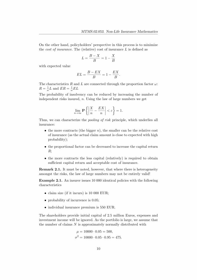
Example 2.1. An insurer issues 10 000 identical policies with the followingcharacteristics
• claim size (if it incurs) is 10 000 EUR;
• probability of incurrence is 0.05;
• individual insurance premium is 550 EUR.
The shareholders provide initial capital of 2.5 million Euros, expenses andinvestment income will be ignored. As the portfolio is large, we assume thatthe number of claims N is approximately normally distributed with
µ = 10000 · 0.05 = 500,
σ2 = 10000 · 0.05 · 0.95 = 475.
10

MTMS.02.053. Non-Life Insurance Mathematics
Thus the incoming cash flow is 550 · 10000 + 2500000 = 8000000 EUR andthe probability of insolvency ε can be calculated as
ε = P{X > 8000000} = P{N > 800} = 1− Φ(13.765) ≈ 0.
The expected cost of insurance is EL = 1 − EXB = 1 − 5000000
5500000 ≈ 0.09 andthe expected return of capital is ER = EL
ω = 0.090.45 = 0.2.
Remark 2.2. Besides the general pooling principle, several risk mitigationtechniques are used in order to manage the insurance risk:
• diversification involves accepting risks that are not similar in order tobenefit from the lessened correlation of contingent events;
• hedging involves accepting risks with a strong negative correlation;
• reinsurance means transferring risks or parts of risks to a reinsurer.
References
1. Booth P., Chadburn, R., Cooper, D., Haberman, S., James, D. (1999)Modern Actuarial Theory and Practice. Chapman & Hall / CRC.
2. Daykin, C.D., Pentikainen, T., Pesonen, M. (1994) Practical Risk The-ory for Actuaries. Chapman & Hall, London.
11

MTMS.02.053. Non-Life Insurance Mathematics
3 Principles of the compensation calculation. Prin-ciples of the deductible
The calculation of compensation relies mainly on the following two charac-teristics:
• insurable value V – describes the value of the insurable object;
• sum insured S – usually determines the limit of the compensation.
The insurable value simply means the value of the insured object. When aninsurance claim occurs, one typically calculates the insurable value immedi-ately before the claim event.
In many classes of property insurance, a sum insured is specified. In mostcases this is an upper limit for the compensation the insurance company willpay in the event of claim.
Both sum insured and insurable value can be given as a fixed sum or as acalculation principle (reinstatement value, replacement value, regular value,etc). If the insurable value and sum insured are both given as fixed sums,these sums regularly need to be equal. Otherwise we are talking about under-insurance (if S < V ) or over-insurance (if S > V ).
If a policyholder suffers a loss caused by an event covered by the insurance,then he receives compensation from the insurer. In the following we introducethe main principles used to calculate the compensation.
Let X be the actual loss and let g(X) denote the calculated compensation.One should be noted that the calculated compensation is not yet the com-pensation that the policyholder actually receives, it is usually reduced by adeductible (this will be described later).
1. Pro-rata principle:
g(x) = min{1, SV} · x,
takes into account the specifics of over- and under-insurance. The com-pensation is reduced proportionally by the ratio between the sum in-sured and the insurable value.
2. First risk principle:g(x) = min{x, S},
the loss is fully covered as long as it does not exceed the sum insured;if it exceeds the sum insured, then the sum insured is covered. Thefirst risk principle is often used when it is difficult to determine aninsurable value.
12
MTMS.02.053. Non-Life Insurance Mathematics
3. Full insurance principle:g(x) = x,
is rarely used, the possible compensation is not limited.
In most cases the calculated compensation is reduced by a deductible.
There are several reasons for introducing deductibles:
a) loss prevention – to lower the probability of claim occurrence;
b) loss reduction – to lower the claim amount in case of a loss event;
c) avoidance of small claims (as administration cost are dominant whenhandling small claims);
d) premium reduction – the first three properties clearly simplify theinsurer’s risk management, in return the insurer can decrease the in-surance premium.
Let h[g(X)] denote the actual compensation paid to the claiming policy-holder. There are 3 main principles of deductibles that can be applied.
A. Fixed amount deductible b:
h1(g(x)) = max{0; g(x)− b}.
B. Proportional deductible β:
h2(g(x)) = (1− β)g(x).
C. Franchise deductible d:
h3(g(x)) = I{g(x)≥d}g(x).
Remark 3.1. Notice that
• principle A satisfies all requirements a)–d);
• principle B could not avoid the handling of small claims c);
• principle C does not satisfy b) and can work against it.
References
1. Booth P., Chadburn, R., Cooper, D., Haberman, S., James, D. (1999)Modern Actuarial Theory and Practice. Chapman & Hall / CRC.
2. Sundt, B. (1993) An Introduction to Non-Life Insurance Mathematics.VVW, Karlsruhe.
13
MTMS.02.053. Non-Life Insurance Mathematics
4 Premium principles
4.1 Desirable properties of premium principles. Classical pre-mium principles
As discussed before, insurance can be considered as transfer of a risk Xfrom policyholder to the insurer. The risk is of stochastic nature, so we canconsider it as a random variable. By the construction, we also assume it is anon-negative random variable; risks taking negative values are not realisticin non-life insurance.
The insurance industry exists because people are willing to pay a price forbeing insured. A natural question related to the insurance process is howmuch should the insurer ask for transfer of a risk X? In other words, weneed to specify some rules to determine a proper premium for a risk X. Apremium principle is a rule H that to any risk X assigns a premium H(X).The premium H(X) is non-random and can be considered as a function ofthe distribution of X.
Before finding some suitable functions H, let us think what properties shouldsuch function have. A short list of natural properties is the following:
1) subadditivity: ∀X,Y , H(X + Y ) ≤ H(X) +H(Y );
2) monotonicity: ∀X,Y , H(X) ≤ H(X + Y );
3) risk loading: ∀X, H(X) ≥ EX;
4) premium is limited by maximal possible loss:for ∀X the inequality P{X < H(X)} < 1 holds;
4’) a weaker form of 4):if ∀X ∃m so that P{X ≤ m} = 1, then also H(X) ≤ m.
Four commonly used classical premium principles are
(a) expected value principle H1(X) = (1 + α)EX, α > 0;
(b) standard deviation principle H2(X) = EX + β√V arX, β > 0;
(c) variance principle H3(X) = EX + γV arX, γ > 0;
(d) “combined variational principle” (compromise principle)H4(X) = EX+β1
√V arX + γ1V arX, β1, γ1 > 0.
Turns out that the some of the properties 1)-4’) are not well satisfied bythese classical principles (prove it!).
14

MTMS.02.053. Non-Life Insurance Mathematics
One can also find premium as a solution for the following condition
P{X ≥ H} ≤ ε,
where ε > 0 is the maximal tolerated ruin probability. In other words, wewant to find a premium which ensures that the probability that this premiumis sufficient to cover the claims is at least 1− ε. In that case we obtain
(e) the quantile principle: H5(X) = minH [P{X ≤ H} ≥ 1− ε].
The quantile premium calculation principle is often also called the percentileprinciple. No additional assumptions are set to risk X, but the amount ofdata must be sufficient to give usable estimates for the required quantiles.
4.2 Utility theory
There is an economic theory that explains how much insureds are willing topay for transferring a possible loss. The theory postulates that a decisionmaker, generally without being aware of it, attaches a value u(x) to hiswealth x instead of just x, where u(·) is called his or her utility function. So,all decisions related to random losses are done by comparing the expectedchanges in utility. Although it is impossible to determine a person’s utilityfunction exactly, we can give some plausible properties of it. For example,more wealth would imply a higher utility level, so the utility function u(·)should be a non-decreasing function. It is also logical that ”reasonable”decision makers are risk averse, which means that they prefer a fixed lossover a random loss with the same expected value. In conclusion, a utilityfunction u(x) is assumed to be increasing (u′(x) > 0) and concave, i.e. therelative value of money will decrease while x increases (u′′(x) < 0).
Maximum premium H that the insured with wealth x is willing to pay isthe solution of the following equation:
u(x−H) = E[u(x−X)].
Similar line of argument applies from an insurer’s viewpoint. Then the min-imum acceptable premium by insurer with utility function u(x) is foundfrom:
u(x) = E[u(x+H −X)].
The problem is that, in general, the premium will depend on the insurer’ssurplus x, which makes it very difficult to apply in practice.
A known solution to last equation is given by function
u(x) =1
a(1− e−ax), a > 0.
15

MTMS.02.053. Non-Life Insurance Mathematics
Using this function we can calculate the premium:
1
a(1− e−ax) =
1
aE(1− e−a(x+H−X));
e−ax = e−axe−aHEeaX ;
eaH = EeaX ;
H =1
alnEeaX .
Thus, we obtained a formula where the premium does not depend on surplusx anymore. The corresponding premium principle is called
(f) exponential principle: H6(X) = 1a lnEeaX .
The parameter a > 0 is called risk aversion, it represents the ’unwilling-ness’ of the insurer to undertake the risk. It can be proved that exponentialpremium increases when a increases: the more risk averse one is, the largerpremium one is willing to pay.
Turns out that the exponential principle satisfies the properties 1)-4’) muchbetter than the classical principles described above (prove it!). Unfortunatelyit has a quite complex form and it is quite difficult to apply this principlein practice.
Remark 4.1 (Allais paradox (1953)). Consider the following capital claims
X = 1 000 000 with probability 1
Y =
5 000 000 with probability 0.10
1 000 000 with probability 0.89
0 with probability 0.01
V =
{1 000 000 with probability 0.11
0 with probability 0.89
W =
{5 000 000 with probability 0.10
0 with probability 0.90
Turns out that having a choice betweenX and Y , many people chooseX, butat the same time they prefer W over V . One can easily see that, assuming aninitial wealth of 0, these choices contradict the expected utility hypothesis. Itseems that the attraction of being completely safe is tronger than expectedutility indicates, and induces people to make irrational decisions.
16

MTMS.02.053. Non-Life Insurance Mathematics
4.3 A note on terminology
The premiums are used in different contexts and with different meanings(depends on how many factors are taken into account). A short overview isgiven by the following list.
• Pure premium: the expected loss EX;
• Risk premium: pure premium EX plus risk loading D, where D iscalculated depending on chosen premium principle;
• Gross premium: risk premium plus expense loading ;
GP =1
1− k· [H(X) +K],
where k denotes expenses proportional to premium (e.g. commissionfees) and K denotes other (unproportional) expenses (e.g. expensesrelated to claim handling and adjustment);
• Net premium: by this we usually mean net of reinsurance (and agent’scommissions or other related costs), i.e. either risk premium minus pay-ments made for reinsurance or gross premium minus payments madefor reinsurance, depending on situation.
We are mainly speaking of risk premiums unless specified otherwise.
References
1. Dickson, D.C.M. (2006) Insurance Risk and Ruin. Cambridge Univer-sity Press.
2. Gray, R.J. & Pitts, S.M. (2012) Risk Modelling in General Insurance.From Principles to Practice. Cambridge University Press.
3. Kaas, R., Goovaerts, M., Dhaene, J., Denuit, M. (2008) Modern Actu-arial Risk Theory: Using R. Springer, Berlin/Heidelberg.
4. Straub, E. (1988) Non-Life Insurance Mathematics. Springer-Verlag /Association of Swiss Actuaries, Berlin/Heidelberg.
5. Sundt, B. (1993) An Introduction to Non-Life Insurance Mathematics.VVW, Karlsruhe.
17

MTMS.02.053. Non-Life Insurance Mathematics
5 Loss distributions
The aim of this chapter is to give a brief overview of distributions suitableto describe the claim severity. Claim severity refers to the monetary lossof an (individual) insurance claim. Obviously the final aim of an insurancecompany is to estimate the aggregate claim amount in order to find suitablepremiums and reserves. The study of individual claims can be seen as thefirst step towards this objective.
5.1 Characteristics of loss distributions
Claim severity is usually modelled as a nonnegative continuous random vari-able.
The list of possible distributions is large:
• Exponential distribution
• Pareto distribution
• Weibull distribution
• Lognormal distribution
• Gamma distribution
• Burr distribution
• Loggamma distribution
• Generalized Pareto distribution
• Inverse Gaussian distribution
• ...
In the following we focus on the first five, i.e. exponential, Pareto, Weibull,lognormal and gamma distributions and give a review of their key charac-teristics.
5.1.1 Exponential distribution
Exponential distribution is a good reference distribution for examples, butusually too ”optimistic” for real models. Exponential distribution is alsooften used to describe the inter-arrival times of loss events. For an exponen-tially distributed random variable X we write X ∼ Exp(λ), where λ > 0 isa parameter.
Main characteristics for the exponential distribution are:
18

MTMS.02.053. Non-Life Insurance Mathematics
• distribution function FX(x) = 1− e−λx, x ≥ 0,
• density function fX(x) = λe−λx, x ≥ 0,
• expectation EX = 1λ ,
• variance V arX = 1λ2
.
5.1.2 Pareto distribution
The Pareto distribution is a power law probability distribution that is usedin several models in economics and social sciences. The corresponding dis-tribution family is a wide one, with several sub-families. We will first reviewthe classical Pareto distribution and then focus on it’s shifted version (so-called American Pareto distribution), which is most widely used in non-lifeinsurance as a model for claim severity.
A. The classical Pareto, X ∼ Pa∗(α, β), α, β > 0
Main characteristics for the classical Pareto distribution are:
• distribution function FX(x) = 1−(βx
)α, x ≥ β,
• density function fX(x) = αβα
xα+1 , x ≥ β,
• expectation EX = αβα−1 , α > 1,
• variance V arX = αβ2
(α−1)2(α−2), α > 2,
• moments EXn = αβn
α−n , α > n, but EXn =∞, α ≤ n.
B. American Pareto, Y ∼ Pa(α, β), Y = X−β, X ∼ Pa∗(α, β), α, β > 0
The American Pareto distribution is obtained from classical Pareto distri-bution by shifting it to the origin.
Main characteristics for the American Pareto distribution are:
• distribution function FY (y) = 1−(
ββ+y
)α, y ≥ 0,
• density function fY (y) = αβα
(β+y)α+1 , y ≥ 0,
• expectation EY = βα−1 , α > 1,
• variance V arY = αβ2
(α−1)2(α−2), α > 2,
• moments EY n = βnn!∏ni=1(α−i) , α > n, but EY n =∞, α ≤ n.
19

MTMS.02.053. Non-Life Insurance Mathematics
Parameter estimation using the method of moments:
α =2(m2 −m2
1)
m2 − 2m21
,
β =m1m2
m2 − 2m21
,
where m1 =∑n
j=1yjn and m2 =
∑nj=1
y2jn .
5.1.3 Weibull distribution
The Weibull distribution is one of the main distributions in survival analysisand reliability analysis, it is also used in models for service and manufac-turing times. Because of its shape it is also usable to model severities innon-life insurance. For a Weibull-distributed random variable X we writeX ∼W (α, λ), α > 0, λ > 0.
Main characteristics for the Weibull distribution are:
• distribution function FX(x) = 1− e−λxα ,
• density function fX(x) = αλαxα−1e−λxα,
• moments EXn = λnΓ(1+nα ).
We also note that if
α < 1, then Weibull distribution is “between” exponential and Pareto;α > 1, then Weibull distribution has lighter tail than exponential;α = 1, then Weibull distribution reduces to exponential.
5.1.4 Lognormal distribution
The distribution function of lognormal distribution is found using the logtransformation to reach normal distribution and standardization to reachstandard normal distribution. Since the normal distribution is one of themost thoroughly studied distributions, the simple connection between log-normal and normal makes lognormal distribution also an appealing choice indifferent models. For a lognormally distributed random variable X we writeX ∼ LnN(µ, σ), −∞ < µ <∞, σ > 0.
Main characteristics are:
• its connection to normal distribution, if Y ∼ N(µ, σ) and X = eY ,then X = LnN(µ, σ),
• distribution function FX(x) = FY (lnx) = Φ( lnx−µσ ),
20

MTMS.02.053. Non-Life Insurance Mathematics
• density function fX(x) = 1xfY (lnx),
• expectation EX = eµ+σ2
2 ,
• variance V arX = e2µ+σ2(eσ
2 − 1),
• moments EXn = enµ+ 12n2σ2
.
Parameter estimation:
µ =1
n
n∑j=1
lnxj ,
σ2 =1
n− 1
n∑j=1
[ln(xj − µ)]2.
5.1.5 Gamma distribution
The gamma distribution can also be considered as a generalization of expo-nential distribution. Namely, if α is integer, then gamma distribution canbe interpreted as a sum of α independent exponentially distributed randomvariables. Gamma distribution is widely used in different models for manu-facturing processes and telecommunications, because of its shape it is alsoa suitable choice in risk and ruin theory. For a gamma-distributed randomvariable X we write X ∼ Γ(α, λ), α > 0, λ > 0.
Main characteristics are:
• distribution function FX(x) = γ(α, xλ),
• density function fX(x) = λα
Γ(α)xα−1e−λx, x > 0,
where
Γ(α) =
∫ ∞0
xα−1e−xdx = (α− 1)Γ(α− 1) is gamma function,
γ(α, t) =
∫ t0 x
α−1e−xdx
Γ(α)is incomplete gamma function,
• expectation EX = αλ ,
• variance V arX = αλ2
.
21
MTMS.02.053. Non-Life Insurance Mathematics
Parameter estimation using the method of moments:
α =m2
1
m2 −m21
,
λ =m1
m2 −m21
.
5.1.6 Mixture distributions. Exponential/Gamma example
Mixture distributions
a) enable us to include in models for claim amounts the variability amongstrisks in a portfolio (that is, they allow us to model heterogeneity ofrisks);
b) provide a source of further heavy-tailed loss distributions;
c) shed further light on some distributions we have already met.
Let us consider the following model:
• size of each individual claim is exponentially distributed;
• parameter of this exponential distribution is a Gamma-distributed ran-dom variable, Λ ∼ Γ(α, β);
• parameters α and β are known.
So, for each fixed λ the (conditional) individual claim size is
X|Λ = λ ∼ Exp(λ)
and the density function of Λ is
fΛ(λ) =βα
Γ(α)λα−1e−βλ, λ > 0.
22

MTMS.02.053. Non-Life Insurance Mathematics
Let us calculate the (marginal) distribution of X:
fX(x) =
∫ ∞0
fX,Λ(x, λ)dλ
=
∫ ∞0
fΛ(λ)fX|Λ(x|λ)dλ
=
∫ ∞0
βα
Γ(α)λα−1e−βλ · λe−λxdλ
=βα
Γ(α)
∫ ∞0
λαe−(x+β)λdλ
=βα
Γ(α)
∫ ∞0
fΓ(λ)Γ(α+ 1)
(x+ β)α+1dλ
=βα
Γ(α)
Γ(α+ 1)
(x+ β)α+1
∫ ∞0
fΓ(λ)dλ
=αβα
(x+ β)α+1,
where Γ ∼ Γ(α+ 1, x+ β).
In conclusion, loss size in this case is (American) Pareto-distributed, X ∼Pa(α, β), i.e. Pareto distribution is a mixture of exponential distributionswith a Gamma mixing distribution.
5.2 Related functions in R statistical software
In R statistical software, there is a variety of functions available related todifferent probability distributions. Some most commonly needed for expo-nential distribution (available in package stats, rate = λ) are:
• dexp(x, rate = 1, log = FALSE) – density;
• pexp(q, rate = 1, lower.tail = TRUE, log.p = FALSE) – distri-bution function;
• qexp(p, rate = 1, lower.tail = TRUE, log.p = FALSE) – quan-tile function;
• rexp(n, rate = 1) – random number generation .
Similar functions are available for all distributions discussed:
• Pareto: dpareto, ppareto, qpareto, rpareto (package actuar);
• Weibull: dweibull, pweibull, qweibull, rweibull (package stats);
• Lognormal: dlnorm, plnorm, qlnorm, rlnorm (package stats);
• Gamma: dgamma, pgamma, qgamma, rgamma (package stats).
23

MTMS.02.053. Non-Life Insurance Mathematics
5.3 Model evaluation and selection
After a distribution has been estimated, we have to evaluate it to ascertainthat the assumptions applied are acceptable and supported by the data.This should be done prior to using the model for prediction and pricing.Model evaluation can be done using graphical methods, as well as formalmisspecification tests and diagnostic checks.
In graphical methods, one simply plots the proposed candidate distribu-tion function against the empirical distribution function. If the proposedcandidate distribution fits well, the plotted graphs should be close, if theproposed distributional assumption is incorrect, the plotted graphs will dif-fer. Similarly, one can plot the probability density functions of candidatedistributions against the histogram of observed data and compare their fit.
Formal misspecification tests can be conducted to compare the estimatedmodel against a hypothesized model. When the key interest is the com-parison of the distribution functions, we may use the Kolmogorov-Smirnovand/or Anderson-Darling test. The chi-square goodness-of-fit test is an al-ternative for testing distributional assumptions, by comparing the observedfrequencies against the theoretical frequencies. The likelihood ratio test isapplicable to test the validity of restrictions on a model, and can be used todecide if a model can be simplified.
We will study two less known methods which might be particularly usefulin insurance related problems:
• method of empirical mean excess function (or mean residual life func-tion);
• limited expected value comparison test.
5.3.1 Method of mean excess function
Let X be a continuous random variable and let x > 0.
Definition 5.1 (Mean excess function e(x)).
e(x) = E(X − x|X ≥ x) =
∫∞x (t− x)fX(t)dt
P{X ≥ x}.
Assuming limt→∞(x− t)(1− FX(t)) = 0, we can also write
e(x) =
∫∞x (1− FX(t))dt
1− FX(x).
24

MTMS.02.053. Non-Life Insurance Mathematics
Empirical mean excess function can be calculated as:
en(x) =n∑i=1
I{xi≥x}xi
#{xi ≥ x}− x.
Mean excess function is used
• in various risk and extreme value models;
• for distribution fitting;
• tail estimation of heavy-tailed distributions;
• ...
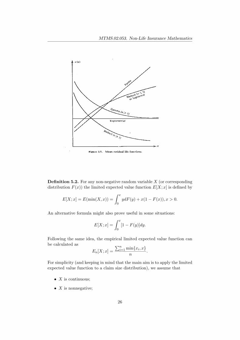
Mean excess functions for the distributions discussed in this chapter havethe following forms:
• X ∼ Pa(α, β), e(x) = β+xα−1 ;
• X ∼ Exp(λ), e(x) = 1λ ;
• X ∼ Γ(α, λ), e(x) ≈ const, if x is large;
• X ∼W (α, λ), e(x) ≈ 1λxα−1 , if x is large;
• X ∼ LN(µ, σ), e(x) ≈ const·xlnx , if x is large.
Graphs of these functions are shown in the next figure. As one can see,the graphs of different distributions are clearly distinguished. So one cansimply calculate the empirical mean excess function and decide based onits behaviour. If this seems like a linear function with positive slope, thena Pareto distribution might be an appropriate model. If it is more like aconstant for the larger x values, gamma might provide good fit. Somethingbetween these choices might suggest either lognormal or Weibull distribu-tion.
5.3.2 Limited expected value comparison test
Another ad hoc test that actuaries sometimes use is closely related to meanexcess functions. This test might be preferred in situations in which the datais censored (from above) and therefore follows certain truncated distribution.Also, in that case it is impossible to compute the empirical mean excessfunction for the tail part.
25
MTMS.02.053. Non-Life Insurance Mathematics
Definition 5.2. For any non-negative random variable X (or correspondingdistribution F (x)) the limited expected value function E[X;x] is defined by
E[X;x] = E(min(X,x)) =
∫ x
0ydF (y) + x(1− F (x)), x > 0.
An alternative formula might also prove useful in some situations:
E[X;x] =
∫ x
0[1− F (y)]dy.
Following the same idea, the empirical limited expected value function canbe calculated as
En[X;x] =
∑ni=1 min{xi, x}
n.
For simplicity (and keeping in mind that the main aim is to apply the limitedexpected value function to a claim size distribution), we assume that
• X is continuous;
• X is nonnegative;
26
MTMS.02.053. Non-Life Insurance Mathematics
• EX <∞.
It is easy to prove that the LEV-function E[X;x] has the following generalproperties:
1. E[X;x] is continuous, concave and nondecreasing function;
2. E[X;x]→ E(X), if x→∞;
3. F (x) = 1− (E[X;x])′
⇒ E[X;x] determines the distribution of X uniquely!
4. Limited expected value function of aX + b is given by
E[aX + b;x] = aE
[X;
x− ba
]+ b.
The goodness-of-fit of a proposed candidate distribution and the observedsample is measured by the following comparison test. Let us calculate thedifferences
di =E[X;xi]− En[X;xi]
E[X;xi], i = 1, 2, . . . , n− c,
and find the vector ~D = (d1, . . . , dn−c), where c is the number of censoredobservations. For simplicity we assume that the sample is ordered and thelast c have not been observed. If ~D is close to null vector, it is reasonable tobelieve that the distribution corresponding to E[X;x] fits given data. Themain problem concerning this method is that there are no good criteria todecide when ~D is close enough to null vector (and when not).
5.4 Effects of coverage modifications to loss distributions
We use the following notations for quantities of interest (also certain sub-scripts may be used to specify the particular situation):
• X – actual loss size, this will be divided between insurer and policy-holder, X = Y + Z;
• Y – insurer’s part of loss;
• Z – policyholder’s part of loss;
• FX(·) – distribution function of X;
• fX(·) – probability density function of X.
27

MTMS.02.053. Non-Life Insurance Mathematics
Let us also define a characteristic that shows the proportion of losses thatgiven coverage limitation (e.g., deductible or an upper limit) allows us toeliminate.
Definition 5.3 (Loss elimination ratio (LER)).
LER =amount of eliminated claims
amount of total claims=
∑Zi∑Xi.
The following examples show how the expected claim amounts change andwhat are loss elimination ratios using different coverage limitations.
Example 5.1. In case of fixed amount deductible b, we can express theactual loss size as a sum
X = Yb + Zb,
where
Yb =
{X − b, if X > b,
0, if X ≤ b.
Then
E(Zb) =
∫ b
0yfX(y)dy + b[1− FX(b)] = E[X; b],
E(Yb) = E(X)− E[X; b]
and
LERb =E[X; b]
E(X).
Example 5.2. If we apply fixed amount deductible and also take into ac-count the inflation rate r, we get the following formulas:
Xr = (1 + r)X,
Yb,r =
{Xr − b, if Xr > b,
0, if Xr ≤ b,
E(Yb,r) = (1 + r)
(E(X)− E
[X;
b
1 + r
]),
LERb,r =E[X; b
1+r
]E(X)
.
If the deductible is not adjusted by inflation, then
• it is not possible to calculate En[X; b1+r ],
28

MTMS.02.053. Non-Life Insurance Mathematics
• LERb,r increases if r increases.
Example 5.3. In case we apply an upper limit u to an individual claimamount, we get the following formulas:
Yu =
{X, if X ≤ u,u, if X > u,
E(Yu) =
∫ u
0xfX(x)dx+ u[1− FX(u)] = E[X;u],
LERu =E(X)− E[X;u]
E(X)= 1− E[X;u]
E(X).
Example 5.4. In case we apply an upper limit u and also adjust by inflationrate r, then:
Xr = (1 + r)X,
E(Yu,r) = (1 + r)E
[X;
u
1 + r
],
LERu,r = 1−E[X; u
1+r
]E(X)
.
If we also adjust the upper limit by inflation, i.e., u′
= (1 + r)u, the expec-tation is calculated as follows:
E(Xu′ ,r) = (1 + r)E
[X;
u′
1 + r
]= (1 + r)E[X;u].
Example 5.5. In case the coverage is modified by upper limit and de-ductible, then, without the effect of inflation we have:
E(Yb,u) = E[X;u]− E[X; b],
=
∫ u
bydF (y) + u(1− F (u))− b(1− F (b)) =
∫ u
b(1− F (y))dy,
LERb,u = LERb + LERu = 1− E[X;u]− E[X; b]
E(X).
If we also take the inflation into account, these formulas change to:
E(Yb,u,r) = (1 + r)
(E
[X;
u
1 + r
]− E
[X;
b
1 + r
]),
LERb,u,r = LERb,r + LERu,r = 1−E[X; u
1+r
]− E
[X; b
1+r
]E(X)
.
29

MTMS.02.053. Non-Life Insurance Mathematics
References
1. Goulet, V., et al. Package ’actuar’: http://cran.r-project.org/
web/packages/actuar/actuar.pdf
2. Gray, R.J. & Pitts, S.M. (2012) Risk Modelling in General Insurance.From Principles to Practice. Cambridge University Press.
3. Hogg, R. & Klugman, S. (1984) Loss distributions. Wiley, New York.
4. R Core Team. Documentation for package ’stats’: http://stat.ethz.ch/R-manual/R-patched/library/stats/html/00Index.html
5. Tse, Y.-K. (2009) Nonlife Actuarial Models. Cambridge UniversityPress.
30

MTMS.02.053. Non-Life Insurance Mathematics
6 Risk models
The aggregate loss of a portfolio of insurance policies is the sum of all lossesincurred in the portfolio. There are two main approaches to model such loss:the individual risk model and the collective risk model.
6.1 Individual risk model
Individual risk model is mostly used in case of group insurance (with fixedgroup size), it is also more common in health and life insurance. In theindividual risk model we consider a risk portfolio with n policies. We alsodenote
• Xk – claim amount corresponding to k-th policy (in case there occursa loss);
• Yk – risk outcome corresponding to k-th policy (0 or Xk);
• S – aggregate (total) claim amount.
The general assumptions for individual risk model are:
1) risks Yk are independent;
2) number of risks n is fixed;
3) each risk Yk can cause at most 1 claim;
4) claims Xk may come from different distributions.
Thus, the aggregate (or total) claim amount can be calculated as
S = Y1 + . . .+ Yn.
The calculation of expectation and variance for S is obvious due to con-struction:
ES = EY1 + . . .+ EYn
andV arS = V arY1 + . . .+ V arYn.
On the other hand, the distribution of S is usually quite hard to find. Notethat typically most policies have zero loss, so that Yk is zero for these policies.In other words, Y follows a mixed distribution with probability mass at pointzero.
31

MTMS.02.053. Non-Life Insurance Mathematics
Example 6.1. Consider the following portfolio from medical insurance
Coverage Number Expected cost Std. devinsured per insured per insured
Single 786 76 42
Family 592 187 77
Then
ES = 786 · 76 + 592 · 187 = 170 440,
V arS = 786 · 422 + 592 · 772 = 4 896 472.
Using the normal approximation, we can find
FS(x) ≈ Φ(x− 170440
2212.8)
and, e.g.,
P{S > 175000} = 1− FS(175000) = 1− Φ(2.06) = 0.0197.
6.2 Collective risk model
The aims of collective risk model are:
• to describe the distribution of total claim amount with some knowndistribution;
• to include only the policies that actually caused claims (in order toreduce the amount of work).
Thus, we define S as a random sum
S =
N∑i=1
Xi,
where N is a random variable denoting the number of claims.
We also assume that
• the claim severities X1, X2, . . . do not depend on the number of claimsN ;
• for any fixed n the individual claims X1, . . . , Xn are i.i.d. random vari-ables.
32

MTMS.02.053. Non-Life Insurance Mathematics
We can see that if all the risks Yi follow the same distribution, individualrisk model can be considered as a special case of collective risk model withP{N = n} = 1.
Let us now denote the distributions of interest:
• F (x) := P{Xk ≤ x} – distribution of individual claim Xk;
• G(x) := P{S ≤ x} – distribution of total claim amount S.
Then
G(x) = P{S ≤ x} = P
{ ∞⋃k=0
{S ≤ x and N = k}
}
=∞∑k=0
P{S ≤ x and N = k} =∞∑k=0
P{N = k}P{S ≤ x|N = k}
=∞∑k=0
P{N = k}P{X1 + . . .+Xk ≤ x}
=∞∑k=0
P{N = k}F ∗k(x),
where F ∗k denotes the n-fold convolution of F .
Remark 6.1 (Convolution of distributions). Let Xi, i = 1, . . . , k be in-dependent random variables with distributions Pi, then the distribution ofX1+. . .+Xk (say, P ) is called the convolution of distributions Pi. Similar no-tion is used for distribution functions and probability density functions: thedistribution function FX1+...+Xk is called the convolution of (independent)distribution functions FXi and denoted by
FX1+...+Xk = FX1 ∗ FX2 ∗ . . . ∗ FXk .
If Xi-s have same distribution, the corresponding convolution is denoted byF ∗k.
For two independent random variables X and Y :
• in general: FX+Y (s) =∫FX(s− y)dFY (y);
• if X is continuous: fX+Y (s) =∫fX(s− y)dFY (y);
• if both X and Y are continuous: fX+Y (s) =∫fX(s− y)fY (y)dy.
33

MTMS.02.053. Non-Life Insurance Mathematics
We also recall the notion of moment generating function of a random vari-able: for any random variable Z, its moment generating function is definedby
MZ(t) = E(etZ).
The key property of moment generating function is that its n-th order deriva-tive at zero gives n-th raw moment of corresponding random variable, i.e.
EZn = M(n)Z (0).
Let us now focus on the moment generating function of aggregate claimamount S. It can be shown that the moment generating function of aggregateclaim amount MS can be calculated using the moment generating functionof individual claims MX and the moment generating function of the claimnumber MN by the following formula:
MS(t) = MN (lnMX(t)).
Furthermore, this relation allows us to calculate expectation and varianceof aggregate claim amount by
ES = EN · EX,V arS = (EX)2 · V arN + EN · V arX.
We also mention that the construction used to define the aggregate claimamount in collective risk model is actually a special form of definition of acompound distribution.
Definition 6.1 (Compound distribution). Let S =∑N
i=1Xi be a (random)sum of random variables Xi, where Xi are i.i.d. and N⊥Xi. Then S has acompound distribution of N .
The distribution of N is called the primary distribution and the distributionof X (where X follows the same distribution as Xi; since Xi-s are i.i.d. wecan simply use X for brevity) is called the secondary distribution.
There are three classical choices for claim number N :
• binomial distribution (EN = np, V arN = np(1− p), EN > V arN);
• Poisson distribution (EN = V arN = λ);
• negative binomial distribution (EN = α(1−p)p , V arN = α(1−p)
p2, EN <
V arN).
Thus we can talk about compound binomial distribution, compound Poissondistribution and compound negative binomial distribution.
34

MTMS.02.053. Non-Life Insurance Mathematics
6.3 Direct estimation of total claim amount
Besides severity-frequency models it is also possible to estimate the aggre-gate claim amount directly.
There are few different options:
• normal approximation (in case 2 first moments can be estimated):
F (x) ≈ Φ
(x− µσ
);
• normal Power approximation (in case we can also estimate skewnessγ):
F (x) ≈ Φ
(−3
γ+
√9
γ2+ 1 +
6
γ
x− µσ
);
• translated gamma approximation:
– set S = k + Y , where Y = Γ(α, λ) and k is some constant
– set parameters α, λ ja k equal to those of S, i.e. solve
µ = k +α
λ,
σ2 =α
λ2,
γ =2√α.
6.4 Conclusions
The aggregate claim amount S can be estimated
• directly; or
• through distributions of individual claim amount X and claim fre-quency N .
Modelling the aggregate claim amount through distributions of X and Nhas some distinct advantages:
• The expected number of claims changes as the number of insured poli-cies changes. Growth in the volume of business needs to be taken intoaccount.
• The effects of inflation are reflected in the individual losses and aredifficult to take into account on aggregate amounts, especially whendeductibles and policy limits do not depend on inflation.
35

MTMS.02.053. Non-Life Insurance Mathematics
• The impact of changing individual deductibles and policy limits ismore easily studied.
• The impact on claims frequencies of changing deductibles is betterunderstood.
• Data that are heterogeneous in terms of deductibles and limits can becombined to obtain the hypothetical aggregate claim amount distribu-tion (useful when data from several years with different conditions iscombined).
• It is easier to take into account the influence of reinsurance.
• The shape of the distribution of S depends on the shapes of bothdistributions of N and X. The understanding of the relative shapes isuseful when modifying policy details.
6.5 Calculation of aggregate claim amount distribution in R
Function aggregateDist (in package actuar): returns a function to com-pute the distribution function of the aggregate claim amount distribution inany point.
Most important arguments of aggregateDist:
• method – method to be used:
– method="recursive" – Panjer recursion;
– method="convolution" – uses convolutions;
– method="normal" – normal approximation;
– method="npower" – Normal Power approximation;
– method="simulation" – uses simulations from empirical distri-bution;
• model.freq – frequency distribution∗;
• model.sev – severity (individual claim amount) distribution∗.
∗ Exact usage will depend on the choice of the method, see the docu-mentation of package actuar.
36
MTMS.02.053. Non-Life Insurance Mathematics
References
1. Dickson, D.C.M. (2006) Insurance Risk and Ruin. Cambridge Univer-sity Press.
2. Goulet, V., et al. Package ’actuar’: http://cran.r-project.org/
web/packages/actuar/actuar.pdf
3. Gray, R.J. & Pitts, S.M. (2012) Risk Modelling in General Insurance.From Principles to Practice. Cambridge University Press.
4. Klugman, S.A., Panjer, H.H., Willmot, G.E. (1998) Loss Models: FromData to Decisions. Wiley, New York.
5. Panjer, H.H., Willmot, G.E. (1992) Insurance risk models. Society ofActuaries.
6. Tse, Y.-K. (2009) Nonlife Actuarial Models. Cambridge UniversityPress.
37
MTMS.02.053. Non-Life Insurance Mathematics
7 Claim number distribution
In this section we study some distributions suitable to describe the number(or frequency) of claims.
7.1 The (a, b)-class of counting distributions
Definition 7.1 (Counting distribution). A counting distribution is a dis-crete distribution with only non-negative integers in its domain.
We typically use a counting distribution to model the number of occurrencesof a certain event, for example ”number of car accidents in a year”.
Definition 7.2 (The (a, b)-class). The (a, b)-class (or (a, b, 0)-class) is atwo-parameter family of counting distributions that satisfy the followingrecursion:
p(k) = (a+b
k)p(k − 1), k = 1, 2, . . . (7.1)
for some a, b ∈ R. The family is usually denoted by R and a particularcounting distribution with parameters a and b is denoted by R(a, b).
Example 7.1 (Poisson distribution). Let us have N ∼ Po(λ).
Then
p(k) = P{N = k} =λk
k!e−λ, p(k − 1) = P{N = k − 1} =
λk−1
(k − 1)!e−λ.
In conclusion
p(k) =λ
kp(k − 1)
, i.e., a = 0 and b = λ or, equivalently,
N ∼ R(0, λ).
Thus, the region of parameters (a, b) covered by the Poisson distribution is
{(a, b) : a = 0, b > 0}.
Example 7.2 (Binomial distribution). Let us have N ∼ Bin(n, p).
Then
p(k) = Cknpk(1− p)n−k, p(k − 1) = Ck−1
n pk−1(1− p)n−k+1
andp(k)
p(k − 1)=n+ 1− k
k
p
1− p= − p
1− p+n+ 1
k
p
1− p
38

MTMS.02.053. Non-Life Insurance Mathematics
or, equivalently,
p(k) =
(− p
1− p+n+ 1
k
p
1− p
)p(k − 1).
NB! Check what happens if k > n!
Thus a = − p1−p and b = −(n + 1)a and the region of parameters (a, b)
covered by binomial distribution is
{(a, b) : a < 0, b = −ma, m = 2, 3, . . .}.
Example 7.3 (Negative binomial distribution). Let us haveN ∼ NBin(α, p).
Then
p(k) = Ckα+k−1pα(1− p)k, p(k − 1) = Ck−1
α+k−2pα(1− p)k−1
andp(k)
p(k − 1)=
(k + α− 1)(1− p)k
= (1− p) +(α− 1)(1− p)
k.
Thus a = (1−p) and b = (α−1)a and the region of parameters (a, b) coveredby negative binomial distribution is
{(a, b) : 0 ≤ a ≤ 1, b > −a}.
Theorem 7.1 (The (a, b)-class theorem). The class R contains the Poisson,the negative binomial, and the binomial distributions, and these are the onlynon-degenerate members.
Idea of the proof:
1. Previous examples show that the mentioned distributions belong to R
2. Consider the remaining 3 regions separately:
(a) a+ b ≤ 0;
(b) a ≥ 1, a+ b > 0;
(c) a < 0, b 6= −ma for any m = 2, 3, . . .
39

MTMS.02.053. Non-Life Insurance Mathematics
7.2 Examples of collective risk models
Example 7.4 (Compound Poisson model). Let us have N ∼ Po(λ). ThenEN = V arN = λ and MN (t) = exp{λ(et− 1)}, general formulas for MS(t),ES and V arS simplify to
MS(t) = exp{λ(MX(t)− 1)},ES = λEX,
V arS = λV arX + λ(EX)2 = λEX2.
Also E(S − ES)3 = λEX3 (prove it!), thus skewness is given by
η3(S) =E(S − ES)3√
(V arS)3=
λEX3√(λEX2)3
≥ 0,
since X ≥ 0.
Recall now that the sum of independent Poisson distributed random vari-able is also Poisson distributed. Such additivity is obviously very desirableproperty for a compound model to have as well. It is important when es-tablishing the relations between distributions of aggregate claim amountsin different aggregation levels. Therefore the question whether the sum ofindependent compound Poisson random variables also has such property isnaturally of great interest.
Theorem 7.2 (Sum of independent compound Poisson random variables).Let S1, S2, . . . , Sn be independent random variables such that Si is compoundPoisson distributed with parameters λi and Fi(x)). Then S1 + . . . + Sn iscompound Poisson distributed with parameters λ and F (x), where
λ =
n∑i=1
λi and F (x) =1
λ
n∑i=1
λiFi(x).
Proof. Notice that F (x) is a distribution function (it is weighted averageof distribution functions with positive weights which sum to 1). The corre-sponding moment-generating function:
M(t) =
∫ ∞0
etx1
λ
n∑i=1
λifi(x)dx =1
λ
n∑i=1
λi
∫ ∞0
etxfi(x)dx =1
λ
n∑i=1
λiMi(t),
where fi(x) and Mi(x) are the probability density function and moment-generating function corresponding to Fi(x).
40

MTMS.02.053. Non-Life Insurance Mathematics
Let MS(t) denote the moment-generating function for S.Then (as S1, S2, . . . , Sn are independent):
MS(t) = EetS = EetS1+...+tSn =n∏i=1
EetSi .
On the other hand:
EetSi = MS(t) = exp{λi(Mi(t)− 1)},
which implies
MS(t) = exp
{n∑i=1
λi(Mi(t)− 1)
}= exp{λ(M(t)− 1)},
where
λ =
n∑i=1
λi and M(t) =1
λ
n∑i=1
λiMi(t).
Since the moment-generating function determines the distribution uniquely,S is compound Poisson distributed with parameters S and F (x).
In conclusion, with the compound Poisson model the estimation of eachindividual risk in homogeneous classes gives immediately an estimate forthe distribution of total claim amount as well. So it is clearly an appealingchoice to model the aggregate claim amount.
Example 7.5 (Compound binomial model). Let us have N ∼ Bin(n, p),then EN = np, V arN = np(1− p) and MN (t) = (p · et + 1− p)n.
Then
MS(t) = (p ·MX(t) + 1− p)n,ES = npEX,
V arS = npV arX + np(1− p)(EX)2 = npEX2 − np2(EX)2.
The expression for the third central moment is
E(S − ES)3 = npEX3 − 3np3EX2EX + 2np3(EX)3
(prove it!) and skewness is calculated as
η3(S) =npEX3 − 3np3EX2EX + 2np3(EX)3√
(npEX2 − np2(EX)2)3.
NB! Skewness can be either positive or negative!
41
MTMS.02.053. Non-Life Insurance Mathematics
Example 7.6 (Compound negative binomial model). Let us have N ∼NBin(α, p), then EN = α(1−p)
p , V arN = α(1−p)p2
and MN (t) = pα(1 − (1 −p)et)−α.
Then
MS(t) =pα
(1− (1− p)Mx(t))α,
ES =α(1− p)
pEX,
V arS =α(1− p)
pV arX +
α(1− p)p2
(EX)2 =α(1− p)
pEX2 +
α(1− p)2
p2(EX)2.
Skewness is positive, but the exact formula is quite complex.
Lastly, we introduce yet another criterion for fitting the claim number dis-tribution from the (a, b)-class of distributions.
We can rewrite the (a, b)-class condition as
p(k)
p(k − 1)= a+
b
k,
which implies k p(k)p(k−1) = ka+ b.
In other words the quantity k p(k)p(k−1) is a linear function of k.
Moreover, the slope a clearly distinguishes the candidate distributions:
• for Poisson a = 0;
• for binomial a < 0;
• for negative binomial a > 0.
In practice, one can plot
k · p(k)
p(k − 1)= k · policies with k claims
policies with k − 1 claims
against k.
References
1. Gray, R.J. & Pitts, S.M. (2012) Risk Modelling in General Insurance.From Principles to Practice. Cambridge University Press.
42

MTMS.02.053. Non-Life Insurance Mathematics
2. Hesselager, O. (1998) Lecture Notes in Non-Life Insureance Mathe-matics. HCO Tryk, Copenhagen.
3. Klugman, S.A., Panjer, H.H., Willmot, G.E. (1998) Loss Models: FromData to Decisions. Wiley, New York.
4. Tse, Y.-K. (2009) Nonlife Actuarial Models. Cambridge UniversityPress.
43

MTMS.02.053. Non-Life Insurance Mathematics
8 Panjer recursion
Recall that we have obtained the following formula for calculating the dis-tribution function for aggregate claim amount:
G(x) =∞∑n=0
P{N = n}F ∗n(x).
The problem is that this approach is usually not feasible except for certainspecial choices for the claim frequency and claim severity distributions. Inthis section, we take a new approach and assume that all severities arepositive and integer-valued. While this might seem unexpected, in practicethis assumption actually holds: all amounts are measured as multiples ofsome monetary unit!
Now, the probability mass function corresponding to aggregate claim amountis
g(x) = P{S = x} =
∞∑n=0
P{N = n}f∗n(x), x = 0, 1, . . . ,
where
f∗n(x) = P{X1 + . . .+Xn = x} =x∑y=1
f(y)f∗(n−1)(x− y)
and f(x) = P{Xi = x}, x = 1, 2, . . ..
Then the next result allows us calculate all the probabilities g(x) sequen-tially, starting from g(0).
Theorem 8.1 (Panjer recursion). Let S =∑N
i=1Xi, where Xi-s are i.i.d.positive integer-valued random variables independent of N . Let the distribu-tion of N belong to the (a, b)-class of counting distributions.
Then
g(x) = P{S = x} =x∑y=1
(a+
by
x
)f(y)g(x− y), x = 1, 2, 3 . . .
and g(0) = P{N = 0}.
Proof. A. g(0) = P{S = 0} = P{N = 0}, since Xi > 0.
B. Use probability generating function PX(t) = EtX =∑∞
i=0 p(i)ti, p(i) =
P{X = i}It can be proved that PS(t) = PN (PX(t)) and therefore also
P ′S(t) = P ′N (PX(t))P ′X(t).
44
MTMS.02.053. Non-Life Insurance Mathematics
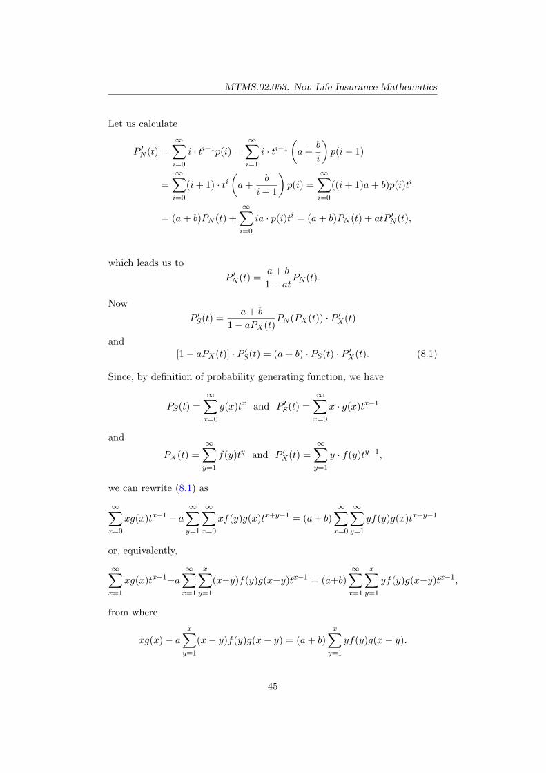
Let us calculate
P ′N (t) =
∞∑i=0
i · ti−1p(i) =
∞∑i=1
i · ti−1
(a+
b
i
)p(i− 1)
=
∞∑i=0
(i+ 1) · ti(a+
b
i+ 1
)p(i) =
∞∑i=0
((i+ 1)a+ b)p(i)ti
= (a+ b)PN (t) +
∞∑i=0
ia · p(i)ti = (a+ b)PN (t) + atP ′N (t),
which leads us to
P ′N (t) =a+ b
1− atPN (t).
Now
P ′S(t) =a+ b
1− aPX(t)PN (PX(t)) · P ′X(t)
and[1− aPX(t)] · P ′S(t) = (a+ b) · PS(t) · P ′X(t). (8.1)
Since, by definition of probability generating function, we have
PS(t) =
∞∑x=0
g(x)tx and P ′S(t) =
∞∑x=0
x · g(x)tx−1
and
PX(t) =∞∑y=1
f(y)ty and P ′X(t) =∞∑y=1
y · f(y)ty−1,
we can rewrite (8.1) as
∞∑x=0
xg(x)tx−1− a∞∑y=1
∞∑x=0
xf(y)g(x)tx+y−1 = (a+ b)
∞∑x=0
∞∑y=1
yf(y)g(x)tx+y−1
or, equivalently,
∞∑x=1
xg(x)tx−1−a∞∑x=1
x∑y=1
(x−y)f(y)g(x−y)tx−1 = (a+b)
∞∑x=1
x∑y=1
yf(y)g(x−y)tx−1,
from where
xg(x)− ax∑y=1
(x− y)f(y)g(x− y) = (a+ b)
x∑y=1
yf(y)g(x− y).
45

MTMS.02.053. Non-Life Insurance Mathematics
In conclusion, we have
g(x) =x∑y=1
(a+
by
x
)f(y)g(x− y), x = 1, 2, 3 . . . .
Now, the probabilities can be calculated sequentially as follows:
• g(1) = (a+ b)f(1)g(0),
• g(2) = (a+ b2)f(1)g(1) + (a+ b)f(2)g(0),
• g(3) = (a+ b3)f(1)g(2) + (a+ 2b
3 )f(2)g(1) + (a+ b)f(3)g(0),
• . . .
Finally, let us note the main advantages of Panjer recursion:
• it is easy to implement;
• it is ”cheaper” than brute-force computation; and
• it allows ”exact” evaluation of compound distributions.
On the other hand, it also has some known weaknesses:
• the method is still still quite resource-expensive, especially in case oflarge number of lattice points;
• precision of the result depends highly on how precise are the estimatesfor distributions of N and X.
References
1. Gray, R.J. & Pitts, S.M. (2012) Risk Modelling in General Insurance.From Principles to Practice. Cambridge University Press.
2. Hesselager, O. (1998) Lecture Notes in Non-Life Insureance Mathe-matics. HCO Tryk, Copenhagen.
46

MTMS.02.053. Non-Life Insurance Mathematics
9 Introduction to classical ruin theory
Recall that while studying the cash-flow model we already encountered thesurplus process of an insurance company in a quite simplified setting. In thissection we study this process more thoroughly.
9.1 Setup
In the classical risk process, an insurer’s surplus at fixed time t > 0 isdetermined by three quantities: the amount of surplus at time 0, the amountof premium income received up to time t, and the amount paid out in claimsup to time t:
U(t) = u+ ct− S(t),
where
• u is the insurer’s initial surplus (at time 0);
• c is the insurer’s (constant) rate of premium income per unit time (forsimplicity it is assumed to be received continuously);
• S(t) is the aggregate claims process.
The aggregate claims process is the only random component in the equality,and is modelled similarly to compound models studied so far:
S(t) =
N(t)∑i=1
Xi,
whereXi are i.i.d. random variables representing the individual claim amountsand {N(t), t ≥ 0} is a counting process for the number of claims.
In the classical risk process model it is assumed that {N(t), t ≥ 0} is aPoisson process and the aggregate claims process {S(t), t ≥ 0} is thus acompound Poisson process.
Definition 9.1. A counting process {N(t), t ≥ 0} is called a Poisson pro-cess, if
(1) N(0) = 0;
(2) the increments of the process N(si + ti) − N(si) are independent fordisjoint intervals (si, si + ti), i = 1, 2, . . .;
47

MTMS.02.053. Non-Life Insurance Mathematics
(3) the distribution of the number of events in an interval of length tis a Poisson distributed random variable with parameter λt, i.e. forarbitrary s, t ≥ 0
P{N(s+ t)−N(s) = n} =(λt)n
n!e−λt, n = 0, 1, 2, . . . .
The quantity λ is called the intensity of the underlying Poisson process.
Definition 9.2. A random process {S(t), t ≥ 0} is called compound Poissonprocess, if
S(t) =
N(t)∑i=1
Xi, t > 0,
where {N(t), t ≥ 0} is a Poisson process and {Xi, i = 1, 2, . . .} are i.i.d.random variables independent of {N(t), t ≥ 0}.
It can be shown that in the Poisson process with intensity λ the interar-rival times (the times between events) are exponentially distributed randomvariables with parameter λ.
In the context of a compound Poisson process representing an aggregateclaims process, for any fixed time t > 0, the distribution of the time untilthe next claim is exponential with parameter λ.
Using the properties of the compound Poisson model, we can see that theaverage growth of the surplus in a time interval with length t is given by
E[U(s+ t)− U(s)] = E[u+ c · (s+ t)− S(s+ t)− u− c · s− S(s)]
= c · t− E[S(s+ t)− S(s)] = c · t− λtEX.
So, in average, the growth of surplus is positive if
c > λEX. (9.1)
The condition (9.1) is called net profit condition and it can be shown thatif this condition does not hold, then ψ(u) = 1 for all u ≥ 0. Therefore, fromnow on we assume that the net profit condition holds, i.e. c > λEX. It isoften convenient to write c = (1 + θ)λEX, where θ is the premium loadingfactor or safety loading :
θ =c
λEX− 1.
So, with net profit condition, we have θ > 0.
48

MTMS.02.053. Non-Life Insurance Mathematics
9.2 Definitions of ruin probability
The probability of ruin in infinite time, also known as the ultimate ruinprobability, is defined as
ψ(u) = P{U(t) < 0 for some t > 0}.
So, ψ(u) is the probability that insurer’s surplus falls below zero at sometime in the future, i.e. the insurer turns insolvent. Given model is a contin-uous time model. For discrete time model, the ultimate ruin probability isexpressed as
ψr(u) = P{U(t) < 0 for some t, t = a, 2a, 3a, . . .}.
If ruin occurs under the discrete time model, it must also occur under thecontinuous time model, the opposite is not true. However, as a becomessmall, so that we are ’checking’ the surplus level very frequently, then ψr(u)should be a good approximation for ψ(u).
One can also define survival probability φ(u), i.e. the probability of non-ruinas
φ(u) = 1− ψ(u).
The finite time ruin probability is defined by
ψ(u, t) = P{U(s) < 0 for some s, 0 < s ≤ t},
i.e., the insurer becomes insolvent at some time in the interval (0, t]. Simi-larly, the discrete time ruin probability in finite time is defined by
ψr(u, t) = P{U(t) < 0 for some s, s = a, 2a, 3a, . . . , t}.
9.3 The adjustment coefficient and Lundberg’s inequality
In order to give an upper bound for the ruin probability, it is importantto measure the risk of given surplus process. This is done using certainadjustment coefficient (or Lundberg exponent) R, which takes into accountthe aggregate claims and the premium income and is defined as the uniquepositive root of the following equality in r:
λMX(r)− λ− cr = 0, (9.2)
where MX(r) is the moment generating function of claim severity X.
In general, the adjustment coefficient equation has one positive solution:
• MX(t) is strictly convex, since M′′X(t) = E(X2etX) > 0;
49

MTMS.02.053. Non-Life Insurance Mathematics
• λMX(t)−λ−ct is decreasing at zero, if net profit condition (9.1) holds,since M
′X(0) = EX < c
λ ;
• MX(t)→∞ continuously (with few exceptions).
There are several equivalent forms to equation (9.2):
• λ+ cR = λMX(R),
• 1 + (1 + θ)R · EX = MX(R),
• eRc = EeRS ,
• c = 1R lnMS(R),
where S is the total claims amount in an interval of length 1 and MS(R) isits moment-generating function.
Theorem 9.1 (Lundberg’s exponential bound for the ruin probability). Fora compound Poisson risk process with an initial capital u, premium per unitof time c, and an adjustment coefficient R, satisfying (9.2) the followinginequality for the ruin probability holds:
ψ(u) ≤ e−Ru.
9.4 Top-down model for premium calculation
The ruin theory also allows us to shed some more light to the premium prin-ciples. Namely, we can use the ruin process model to find certain estimatesfor the risk loading coefficients of premium principles.
Let us start with the following question: how large should be the initialcapital u and the premimum c in order to remain solvent at all times witha prescribed probability?
By the Lundberg inequality, the ruin probability ψ(u) is bounded from aboveby e−Ru, where R can be found as the root of eRc = EeRS . Now, if we setthe upper bound equal to ε, then
R =| ln ε|u
. (9.3)
Hence, the premium c can be calculated for given initial capital u and allowedruin probability ε using the following formula:
c =1
Rln(EeRS), (9.4)
50
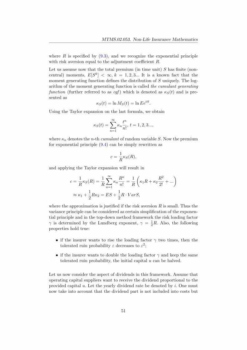
MTMS.02.053. Non-Life Insurance Mathematics
where R is specified by (9.3), and we recognize the exponential principlewith risk aversion equal to the adjustment coefficient R.
Let us assume now that the total premium (in time unit) S has finite (non-central) moments, E[Sk] < ∞, k = 1, 2, 3... It is a known fact that themoment generating function defines the distribution of S uniquely. The log-arithm of the moment generating function is called the cumulant generatingfunction (further referred to as cgf ) which is denoted as κS(t) and is pre-sented as
κS(t) = lnMS(t) = lnEetS .
Using the Taylor expansion on the last formula, we obtain
κS(t) =
∞∑n=1
κntn
n!, t = 1, 2, 3...,
where κn denotes the n-th cumulant of random variable S. Now the premiumfor exponential principle (9.4) can be simply rewritten as
c =1
RκS(R),
and applying the Taylor expansion will result in
c =1
RκS(R) =
1
R
∞∑n=1
κnRn
n!=
1
R
(κ1R+ κ2
R2
2!+ ...
)≈ κ1 +
1
2Rκ2 = ES +
1
2R · V arS,
where the approximation is justified if the risk aversion R is small. Thus thevariance principle can be considered as certain simplification of the exponen-tial principle and in the top-down method framework the risk loading factorγ is determined by the Lundberg exponent, γ = 1
2R. Also, the followingproperties hold true:
• if the insurer wants to rise the loading factor γ two times, then thetolerated ruin probability ε decreases to ε2;
• if the insurer wants to double the loading factor γ and keep the sametolerated ruin probability, the initial capital u can be halved.
Let us now consider the aspect of dividends in this framework. Assume thatoperating capital suppliers want to receive the dividend proportional to theprovided capital u. Let the yearly dividend rate be denoted by i. One mustnow take into account that the dividend part is not included into costs but
51

MTMS.02.053. Non-Life Insurance Mathematics
must be added to them, therefore the premium must be also increased byiu. The risk process (for one year) can then be presented as
U1 = u+ (c+ iu)− S − iu.
Thus, the question to be answered is: how big should the premium be toensure the non-ruin probability 1 − ε and to cover the dividends paid tothe shareholders? Consider the variance premium calculation principle withloading factor γ = 1
2R, where R is calculated as in (9.3). Then the corre-sponding premium can be presented by
H(S) = ES +| ln ε|
2uV arS + iu. (9.5)
Such premium is more likely to be achieved if the initial capital is chosen sothat it makes the premium to be as low as possible. After setting the firstderivative of H(S) with respect to u equal to zero, we get
H ′(S) = −V arS | ln ε|2u2
+ i = 0,
or, equivalently,V arS| ln ε|
2u2= i.
The the initial capital u can be calculated from
u =√V arS
√| ln ε|
2i. (9.6)
To obtain the required premium, the derived initial capital u must be sub-stituted into (9.5). After some simplifications it comes out that the premiumis equal to
H(S) = ES +
√i| ln ε|
√V arS√
2+
√i| ln ε|
√V arS√
2
= ES +√
2i| ln ε|√V arS.
As√V arS is the standard deviation of claim amount S, the derived pre-
mium is the standard deviation premium with the loading factor β =√
2i| ln ε|.Due to (9.6), it can be shown that the following propositions hold for someinitial capital u and dividend rate i:
• the higher the dividend rate i, the higher the dividend part iu;
• the higher is the required dividend rate i, the lower is the optimal sizeof initial capital u.
52

MTMS.02.053. Non-Life Insurance Mathematics
References
1. Dickson, D.C.M. (2006) Insurance Risk and Ruin. Cambridge Univer-sity Press.
2. Kaas, R., Goovaerts, M., Dhaene, J., Denuit, M. (2008) Modern Actu-arial Risk Theory: Using R. Springer, Berlin/Heidelberg.
3. Ross, S.M. (2009) Introduction to Probability Models. Elsevier/AcademicPress.
53

MTMS.02.053. Non-Life Insurance Mathematics
10 Reinsurance
Similarly to ”regular” insurance, the risks and liabilities can grow too highfor a single insurer to handle, thus there is a need to transfer portions of riskportfolios to other parties by some form of agreement in order to reduce thelikelihood of having to pay a large obligation resulting from an insuranceclaim.
There are two general solutions
• reinsurance – ”insurance for insurers”;
• co-insurance – cooperation with other insurers.
In the reinsurance process, the initial insurer is called either ceding companyor cedant or cedent, for the reinsurer we may also use the term reinsurancecompany. An example of the reinsurance process is shown in the followingfigure.
Some world’s biggest names in reinsurance business are Swiss Re, MunichRe, Hannover Re, Lloyd’s, Allianz.
10.1 Types of reinsurance
Reinsurance can be classified by the type of reinsurance contract:
• facultative reinsurance;
• compulsory (treaty) reinsurance.
54

MTMS.02.053. Non-Life Insurance Mathematics
By the compensation mechanics, reinsurance can be divided into the follow-ing categories:
• proportional reinsurance:
– quota share;
– surplus;
• non-proportional reinsurance:
– excess of loss (XL);
– stop loss.
Before studying the reinsurance mechanics in different categories, we needto introduce some related notation. Let us denote
• S,X, P – gross total claim amount, severity, premium;
• S, X, P – net total claim amount, severity, premium;
• S, X, P – reinsurer’s total claim amount, severity, premium.
10.1.1 Proportional reinsurance
The main principle of proportional reinsurance is that the proportion ofpremiums equals to the proportion of claim amount.
Remark 10.1. In practice, this is not entirely true, since there are, in fact,certain commission fees that need to be taken into account separately. Com-mission fee is a fee that the reinsurer pays to ceding company for bringingthe reinsurer a new client. Still, the commission fees do not change the gen-eral principle and are not of interest from our point of view, thus, we maysafely ignore them.
So, we can illustrate the idea of proportional reinsurance by the followingformula:
P
P=X
X.
Main advantage of proportional reinsurance is simple calculation of premi-ums and compensation, while the main drawback is that both parties haveto handle all claims (not depending on claim size).
There are two types of proportional reinsurance. In quota share reinsurance,everything is determined by fixed retention proportion α, 0 < α < 1.
55

MTMS.02.053. Non-Life Insurance Mathematics
Then, all claims in given portfolio are divided using proportion α as follows:
X = αX, X = (1− α)X,
S = αS, S = (1− α)S.
Similar holds for premiums:
P = αP, P = (1− α)P.
Another type of proportional reinsurance is the surplus reinsurance. Whereasquota share reinsurance scales down each risk in the same proportion, a sur-plus treaty is more flexible: the proportion of each risk reinsured may vary.To obtain this flexibility, we need to introduce more parameters than onesingle proportion factor. The ceded amount is defined by the following pa-rameters:
• ceding company retains at most a certain amount m of each risk (oneline);
• the exceeding part is reinsured but only up to a certain multiple l ofthe retention (number of lines);
• proportion of liabilities is determined individually depending on therisk size Q (consider, e.g., possible maximal loss (PML), sum insuredor estimated maximum loss (EML));
• (automatic underwritten) capacity of the treaty is thus L = (l+ 1)m.
• larger risks Q > L will require another reinsurance layer or facultativereinsurance.
Under such construction the initial insurer’s (cedant’s) part is calculated as:
X =
{X, Q ≤ m;mQX, m < Q ≤ L.
NB! The quantities Q and m are fixed when contract is underwritten anddo not depend on the actual claim amount X. If X = Q then X = m, i.e.initial insurer’s maximal payout can not exceed m.
Example 10.1 (Surplus treaty). Consider a 9-line surplus treaty (l1 = 9)with one line m1 = 1 000 000 EUR, i.e. the treaty capacity is L1 = (l1 +1)m1 = 10 000 000 EUR. Let the cedant also have another surplus treatywith m2 = 10 000 000, l2 = 3 and L2 = 40 000 000. Consider a risk suchthat risk size (Q) is 21 million EUR.
56
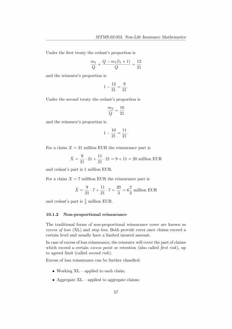
MTMS.02.053. Non-Life Insurance Mathematics
Under the first treaty the cedant’s proportion is
m1
Q+Q−m1(l1 + 1)
Q=
12
21
and the reinsurer’s proportion is
1− 12
21=
9
21.
Under the second treaty the cedant’s proportion is
m2
Q=
10
21
and the reinsurer’s proportion is
1− 10
21=
11
21.
For a claim X = 21 million EUR the reinsurance part is
X =9
21· 21 +
11
21· 21 = 9 + 11 = 20 million EUR
and cedant’s part is 1 million EUR.
For a claim X = 7 milllion EUR the reinsurance part is
X =9
21· 7 +
11
21· 7 =
20
3= 6
2
3million EUR
and cedant’s part is 13 million EUR.
10.1.2 Non-proportional reinsurance
The traditional forms of non-proportional reinsurance cover are known asexcess of loss (XL) and stop loss. Both provide cover once claims exceed acertain level and usually have a limited insured amount.
In case of excess of loss reinsurance, the reinsurer will cover the part of claimswhich exceed a certain excess point or retention (also called first risk), upto agreed limit (called second risk).
Excess of loss reinsurance can be further classified:
• Working XL – applied to each claim;
• Aggregate XL – applied to aggregate claims;
57

MTMS.02.053. Non-Life Insurance Mathematics
• Cat XL – applied to losses occurred in a fixed period after a catastro-phe.
Claims are divided by initial insurer and reinsurer as follows:
X = min(X,M)
andX = max(0, X −M),
where M is the retention of initial insurer.
Usually the XL-treaty covers certain layer A exceeding threshold M (layerA xs M ). In such case
X = min(A,max(0, X −M)) = min(M +A,X)−min(M,X).
In stop-loss contracts the aggregate covers are linked to the cedant’s grosspremium income during a 12 month period (P ) through the loss ratio S
P : incase S
P exceeds a fixed proportion, exceeding part is covered by reinsurer.
Usually the reinsurer’s liability is also limited, i.e. the reinsurer will cover alayer defined by m1 <
SP ≤ m2.
For example m1 = 1.05, m2 = 1.3 Then,
• in case SP ≤ 1.05 everything is covered by cedant, S = S;
• if 1.05 < SP ≤ 1.3 then S = 1.05 · P and S = S − 1.05 · P ;
• if SP > 1.3 then S = S − 0.25 · P and S = 0.25 · P .
Example 10.2. Consider a portfolio with the following risks:
Risks House Block of flats Industry
A 100 000
B 200 000
C 300 000
D 2 000 000
E 10 000 000
F 20 000 000
Premium rate 0.1% 0.2% 0.3%
Losses B: 150 000 F: 2 550 000
Sum insured 600 000 2 000 000 30 000 000
Gross premium 600 4000 90 000
Loss burden 150 000 2 550 000
Consider also the following reinsurance contracts:
58

MTMS.02.053. Non-Life Insurance Mathematics
1. Quota of 30% (i.e. retention α = 70%);
2. Surplus 4 max after 100 000, 500 000, 2 500 000;
3. Fac. 7.5 million after 12.5 million;
4. Excess of loss (WXL) 4 million xs 1 million;
5. Stop loss 8 million after 2 million (Aggregate XL 8 million xs 2 million).
Then the corresponding reinsurance claims and premiums are shown in thefollowing table:
Premiums (P ) Claims (S)
1 28 380 810 000
2 55 800 1 350 000
3 22 500 956 250
4 ? 1 550 000
5 ? 700 000
10.2 The effect of reinsurance to claim distributions
Let us now study how the modifications to the cover by reinsurance affectthe claim distributions.
In case of proportional reinsurance the proportion α fixed (either the samefor all policies in case of quota share, or different for each risk dependingon its size in case of surplus), so the claim severity distribution X is foundfrom:
FX(x) = P{X ≤ x} = P{αX ≤ x} = P{X ≤ x
α} = FX(
x
α).
The number of claims (claim frequency) stays the same for both parties.
In case of non-proportional (XL) reinsurance, the distribution of X = min(M,X)is given by
FX(x) =
{FX(x), x < M,
1, x ≥M.
Then, the expected individual and aggregate claim amounts for initial in-surer are:
EX = E(min(M,X)) = E[X;M ],
ES = ENEX = EN · E[X;M ].
In practice, the reinsurer only needs to know the claims he is (partially)compensating, i.e. claims exceeding M . Therefore we introduce the followingvariables which are important from reinsurer’s point of view:
59

MTMS.02.053. Non-Life Insurance Mathematics
• individual claim size: XM := X −M |X > M ;
• number of claims: NM :=∑N
i=1 I{Xi>M}.
The distribution function corresponding to XM is
FXM (x) : = P{XM ≤ x} = P{X −M ≤ x|X > M}
= P{M < X ≤ x+M |X > M} =
∫ x+MM fX(t)dt
1− FX(M)
=FX(x+M)− FX(M)
1− FX(M), x ≥ 0
and the probability density function of XM is
fXM (x) =fX(x+M)
1− FX(M), x ≥ 0.
By construction, the expectation of XM is
EXM = E(X −M |X > M) = e(M) =EX − E[X;M ]
1− FX(M).
On the other hand, since X + X = X,
EX = EX − EX = EX
(EX − EX
EX
)= EX
(1− E[X;M ]
EX
).
Denote c(x) := 1− E[X;x]EX , then
EXM =c(M) · EX1− FX(M)
=EX
1− FX(M).
Expected number of claims NM can be calculated:
ENM = E(
N∑i=1
I{Xi>M}) = EN(1− FX(M))
In conclusion, the expected total claim amount SM is given by
ESM = EXMENM =EX
1− FX(M)EN(1− FX(M)) = EXEN = ES.
60

MTMS.02.053. Non-Life Insurance Mathematics
References
1. Booth P., Chadburn, R., Cooper, D., Haberman, S., James, D. (1999)Modern Actuarial Theory and Practice. Chapman & Hall / CRC.
2. Gray, R.J. & Pitts, S.M. (2012) Risk Modelling in General Insurance.From Principles to Practice. Cambridge University Press.
3. Straub, E. (1988) Non-Life Insurance Mathematics. Springer-Verlag /Association of Swiss Actuaries, Berlin/Heidelberg.
61

MTMS.02.053. Non-Life Insurance Mathematics
11 Reserving
An insurance company’s technical reserve is the amount set aside to meetcompany’s principal insurance liabilities. Reserves are required in respect ofbusiness written, both earned and unearned.
Technical reserves serve serveral purposes:
• to enable the company to meet and administer its contractual obliga-tions to policyholders;
• to provide management information;
• for tax purposes;
• to assist in sale and purchase negotiations;
• to advise on portfolio reinsurance;
• ...
The reserves held in respect of insurance related liabilities fall into threemain categories:
• reserves in respect of unexpired (or unearned) exposure:
1. unearned premium reserve (UPR);
2. deferred acquisition costs (DAC);
3. additional unexpired risk reserve (AURR);
• contingent reserves:
1. catastrophe reserves;
2. claims equalization reserves;
• reserves in respect of earned exposure:
1. notified outstanding claims (OCR);
2. incurred but not reported claims(IBNR);
3. incurred but not enough reported (IBNER) on existing notifiedclaims.
62

MTMS.02.053. Non-Life Insurance Mathematics
11.1 Unearned premium reserve (UPR)
The situation related to premium payments can be briefly described as fol-lows:
• premiums are paid in advance;
• policies start at different times;
• insurance periods and accounting periods generally do not match;
• the insurer has contractual obligations to provide coverage beyond theaccounting date.
Thus, the following two questions need to be answered:
1. How do estimate the sufficient size of the UPR?
2. When can we say that a premium is finally earned?
In general, the UPR in respect of an individal policy can be expressed usingthe following formula:
UPR(ti) = P0 · F (ti) · (1− k),
where
• ti is the accounting date;
• P0 is the premium received from given policy;
• F (ti) is the proportion of the not exposed cover for this policy;
• k is the proportion of expenses (acquisition expenses are treated asearned).
A straightforward basic formula for the proportion factor is
F (·) =period of unexpired cover
duration of original policy.
Such approach is also called the 1365 -method. Proportions are calculated for
each individual policy.
In practice it is unusual to calculate a UPR on an individual policy basis;generally the premiums received are aggregated within similar classes ofbusiness by month or quarter and the UPR is calculated on the assumptionthat the premiums were received, on average, half way through the period.So we can talk about
63

MTMS.02.053. Non-Life Insurance Mathematics
• monthly (’24ths’ or 124 -) method;
• quarterly (’eights’ or 18 -)method.
Then, the formula corresponding to 124 -method is
F (t) =2t− 1
24, t = 1, 2, . . . , 12.
Similar construction holds for quarterly calculations.
Example 11.1. Let the accounting date be 31.12.2012 and let us considerpolicies that started in March 2012. Then t = 3 and F (3) = 2·3−1
24 = 524 , i.e.
for each policy started in March 2012 a proportion 524 from premiums is still
unearned at the end of year 2012.
In case the risk exposure is not uniformly spread over the policy durationone can
• use a more complex proportion function F (t);
• use additional reserves for periods with higher risk intensity.
11.2 Reserves in respect of earned exposure
The process underlying the appearance of a claim in the insurance company’sbooks involves:
1) the occurrence of an insured event causing a loss to the policyholder;
2) the policyholder being aware of the loss and subsequently advising theinsurer via a claim form;
3) the insurer processing the claim form and establishing a case reservewhich might lead to a payment.
There are different options for establishing and estimation of the claim re-serves:
• straightforward – claim-based approach (for reported claims);
• statistical methods for estimating required future provisions (espe-cially important in IBNR calculation)
– chain ladder method;
– Bornhutter-Ferguson method;
64

MTMS.02.053. Non-Life Insurance Mathematics
– other stochastic approaches (GLM).
The claim development pattern is usually depicted in the following form(run-off triangle):
Development period jYear of origin i 0 1 2 . . . J
0 C00 C01 C02 . . . C0J
1 C10 C11 . . .2 C20 . . .. . . . . .I CI0
Here Cij denotes the claims (numbers or amounts) for year of origin i(i = 0, . . . , I, we can also use simply calendar years here) and developmentyear j (j = 0, . . . , J). Development period 0 means ”current” or ”running”period and the number of development periods J is defined by the nature ofparticular risks. The number of usable years of origin is defined by the his-tory insurance company has. The usual assumption is that I = J ; although,it is possible that the insurance company has more historical informationabout the particular reserve development (I > J), in this case we assumethat all this information is included in the first row of the run-off triangle.
The development pattern is defined by the choice for the year of origin,which can be
• year of underwriting;
• year of claim occurrence;
• year of reporting;
and the development year, which can be
• year of occurrence;
• year of reporting;
• year of claim settlement (year of final payment).
Depending on the choice of years of origin and development, the run-off tri-angles can describe the development of different stages of different reserves.Obviously the development period has to correspond to a later process thanthe year of origin in order to get a meaningful development pattern.
For example
65

MTMS.02.053. Non-Life Insurance Mathematics
• if the development period is the reporting year, the corresponding run-off triangle describes development in IBNR reserve;
• if the development period is the claim settlement year, the correspond-ing run-off triangle describes development in OCR reserve.
11.2.1 The chain ladder method
The most widely used reserving method is the chain ladder method. Thereare many variations, but they all have the same objective: to extract fromthe loss development triangle a pattern for the claim run-off that can beused to extrapolate the less mature years of account. The method is verysimple and is based on the assumption that the development proportionsremain the same (or at least are similar) in the future. If this assumptionholds, the behaviour of future claims behaviour can be described by certaindevelopment factors or, equivalently, through some proportion factors.
More precisely, the chain ladder model assumes that the development be-tween successive periods of development can be described as
Ci,j+1 ≈ fjCij , i = 0, . . . , I, j = 0, . . . , J − 1,
where
• Cij is the (cumulative) claim amount (or number) corresponding toyear of origin i and development period j;
• Ci,j+1 is the (cumulative) claim amount (or number) corresponding toyear of origin i and development period j + 1;
• fj is the development factor between development periods j and j+1.
Equivalently, the chain ladder model can be written as
Cij ≈ SiRj ,
where
• Cij is the (cumulative) claim amount (or number) corresponding toyear of origin i and development period j;
• Si is the ultimate claim amount (or number) for year of origin i;
• Rj is the proportion of the ultimate that has emerged by the end ofthe on jth development period.
66

MTMS.02.053. Non-Life Insurance Mathematics
The approximate equalities are used to stress out that there is no fixedrelationship, we just propose a model for predictions (alternatively, one canspecify a model with exact equalities and include error terms).
The estimation of development factors is done using all the available infor-mation between successive development periods:
fj =
∑I−j−1i=0 Ci,j+1∑I−j−1i=0 Cij
, j = 0, . . . , J − 1.
The cumulative development factors describe development pattern betweengiven development stage j and the ultimate (or final) stage J . Thus, theestimates are found as
Fj =
J−1∏k=j
fk, j = 0, . . . , J − 1.
Also, the inverses of cumulative factors represent the proportion of totalclaims emerged by the end of given development period. Thus, the the esti-mates for proportions are simply found by
Rj =1
Fj, j = 0, . . . , J − 1.
As the basic chain ladder method does not take into account factors depend-ing on particular calendar years (e.g. inflation) the following adjustment canbe made to obtain a more flexible model:
Cij ≈ SiRjλij ,
where λij is the inflation coefficient.
In order to apply the influence of inflation to correct datum it is necessaryto consider incremental data while correcting with inflation, i.e. in first stepwe apply the inflation to increments and in second step we get cumulativesums from inflation-adjusted increments.
The calculation of different reserves using chain ladder method is shown inthe following examples. The key step is step 5 where the development factorsand proportions are found.
67

MTMS.02.053. Non-Life Insurance Mathematics
OCR example - paid claims
0 1 2 3 4 5199119921993199419951996
0 1 2 3 4 5199119921993199419951996
0
0 - 1 1 - 2 2 - 3 3 - 4 4 - 51991 1,547 1,113 1,086 1,050 1,0301992 1,581 1,118 1,075 1,0451993 1,570 1,097 1,0691994 1,479 1,0871995 1,5501996
0 - 1 1 - 2 2 - 3 3 - 4 4 - 51,542 1,102 1,076 1,047 1,030
1,972 1,279 1,160 1,079 1,0300,507 0,782 0,862 0,927 0,971
Step 1 – Incremental paid claimsDevelopment period
Year of origin52 546 28 729 9 186 7 816 4 885 3 10262 285 36 210 11 601 8 250 5 33672 173 41 126 11 041 8 54386 135 41 224 11 05097 068 53 408
128 982
Step 2 – Cumulative paid claimsDevelopment period
Year of origin52 546 81 275 90 461 98 277 103 162 106 26462 285 98 495 110 096 118 346 123 68272 173 113 299 124 340 132 88386 135 127 359 138 40997 068 150 476
128 982Column sum 499 189 570 904 463 306 349 506 226 844 106 264Column sum (excl. last value) 370 207 420 428 324 897 216 623 103 162
Step 3 – Graph
Step 4 – Ratios of cumulative payments in successive development periodsDevelopment period
Year of origin
Step 5 – Chain ladder ratiosDevelopment period
Ratio0 – ultimate 1 – ultimate 2 – ultimate 3 – ultimate 4 – ultimate
Cumulative factorInverse
0 1 2 3 4 50
20 00040 00060 00080 000
100 000120 000140 000160 000
199119921993199419951996
68
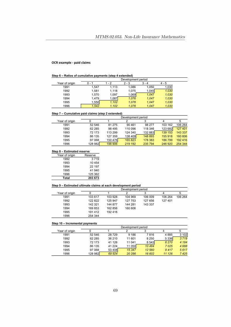
MTMS.02.053. Non-Life Insurance Mathematics
OCR example - paid claims
0 - 1 1 - 2 2 - 3 3 - 4 4 - 51991 1,547 1,113 1,086 1,050 1,0301992 1,581 1,118 1,075 1,045 1,0301993 1,570 1,097 1,069 1,047 1,0301994 1,479 1,087 1,076 1,047 1,0301995 1,550 1,102 1,076 1,047 1,0301996 1,542 1,102 1,076 1,047 1,030
0 1 2 3 4 5199119921993199419951996
Reserve19921993199419951996
0 1 2 3 4 5199119921993199419951996
0 1 2 3 4 5199119921993199419951996
Step 6 – Ratios of cumulative payments (step 4 extended)Development period
Year of origin
Step 7 – Cumulative paid claims (step 2 extended)Development period
Year of origin52 546 81 275 90 461 98 277 103 162 106 26462 285 98 495 110 096 118 346 123 682 127 40172 173 113 299 124 340 132 883 139 153 143 33786 135 127 359 138 409 148 893 155 918 160 60697 068 150 476 165 823 178 383 186 799 192 416
128 982 198 906 219 192 235 794 246 920 254 344
Step 8 – Estimated reserveYear of origin
3 71910 45422 19741 940
125 362Total 203 673
Step 9 – Estimated ultimate claims at each development periodDevelopment period
Year of origin103 617 103 928 104 969 106 009 106 264 106 264122 822 125 947 127 753 127 656 127 401142 321 144 877 144 281 143 337169 853 162 856 160 606191 412 192 416254 344
Step 10 – Incremental paymentsDevelopment period
Year of origin52 546 28 729 9 186 7 816 4 885 3 10262 285 36 210 11 601 8 250 5 336 3 71972 173 41 126 11 041 8 543 6 270 4 18486 135 41 224 11 050 10 484 7 025 4 68897 068 53 408 15 347 12 560 8 417 5 617
128 982 69 924 20 286 16 602 11 126 7 425
69
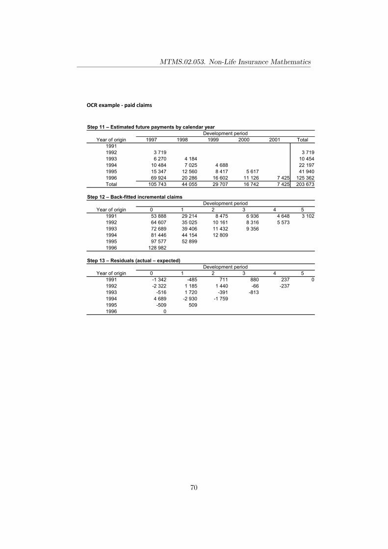
MTMS.02.053. Non-Life Insurance Mathematics
OCR example - paid claims
1997 1998 1999 2000 2001199119921993199419951996
0 1 2 3 4 5199119921993199419951996
0 1 2 3 4 51991 -485 711 880 237 01992 -66 -2371993 -516 -391 -81319941995 -509 5091996 0
Step 11 – Estimated future payments by calendar yearDevelopment period
Year of origin Total
3 719 3 7196 270 4 184 10 454
10 484 7 025 4 688 22 19715 347 12 560 8 417 5 617 41 94069 924 20 286 16 602 11 126 7 425 125 362
Total 105 743 44 055 29 707 16 742 7 425 203 673
Step 12 – Back-fitted incremental claimsDevelopment period
Year of origin53 888 29 214 8 475 6 936 4 648 3 10264 607 35 025 10 161 8 316 5 57372 689 39 406 11 432 9 35681 446 44 154 12 80997 577 52 899
128 982
Step 13 – Residuals (actual – expected)Development period
Year of origin-1 342-2 322 1 185 1 440
1 7204 689 -2 930 -1 759
70
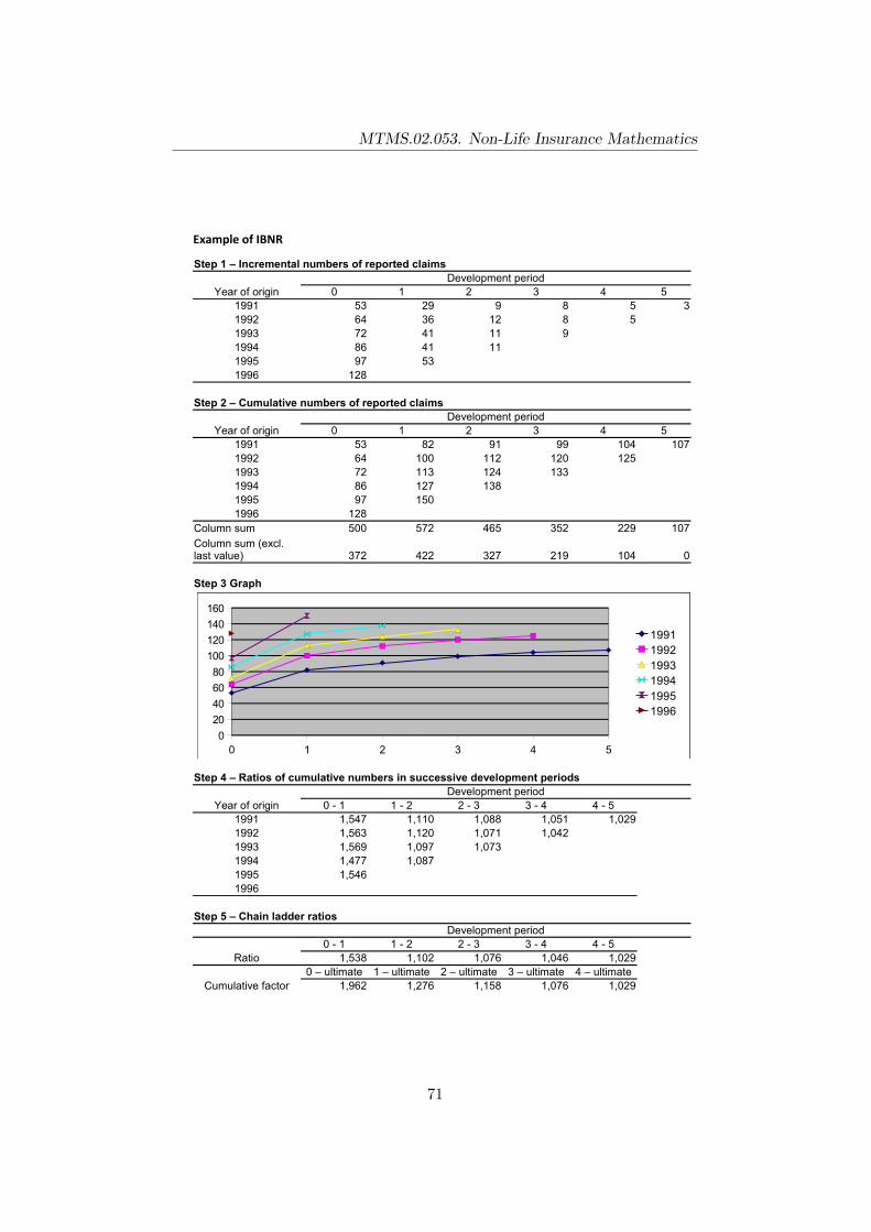
MTMS.02.053. Non-Life Insurance Mathematics
Example of IBNR
0 1 2 3 4 51991 53 29 9 8 5 31992 64 36 12 8 51993 72 41 11 91994 86 41 111995 97 531996 128
0 1 2 3 4 51991 53 82 91 99 104 1071992 64 100 112 120 1251993 72 113 124 1331994 86 127 1381995 97 1501996 128
500 572 465 352 229 107
372 422 327 219 104 0
0 - 1 1 - 2 2 - 3 3 - 4 4 - 51991 1,547 1,110 1,088 1,051 1,0291992 1,563 1,120 1,071 1,0421993 1,569 1,097 1,0731994 1,477 1,0871995 1,5461996
0 - 1 1 - 2 2 - 3 3 - 4 4 - 51,538 1,102 1,076 1,046 1,029
1,962 1,276 1,158 1,076 1,029
Step 1 – Incremental numbers of reported claimsDevelopment period
Year of origin
Step 2 – Cumulative numbers of reported claimsDevelopment period
Year of origin
Column sumColumn sum (excl. last value)
Step 3 Graph
Step 4 – Ratios of cumulative numbers in successive development periodsDevelopment period
Year of origin
Step 5 – Chain ladder ratiosDevelopment period
Ratio0 – ultimate 1 – ultimate 2 – ultimate 3 – ultimate 4 – ultimate
Cumulative factor
0 1 2 3 4 50
20406080
100120140160
199119921993199419951996
71

MTMS.02.053. Non-Life Insurance Mathematics
Example of IBNR
0,510 0,784 0,864 0,930 0,972
0 - 1 1 - 2 2 - 3 3 - 4 4 - 51991 1,547 1,110 1,088 1,051 1,0291992 1,563 1,120 1,071 1,042 1,0291993 1,569 1,097 1,073 1,046 1,0291994 1,477 1,087 1,076 1,046 1,0291995 1,546 1,102 1,076 1,046 1,0291996 1,538 1,102 1,076 1,046 1,029
0 1 2 3 4 51991 53 82 91 99 104 1071992 64 100 112 120 125 1291993 72 113 124 133 139 1431994 86 127 138 149 155 1601995 97 150 165 178 186 1911996 128 197 217 233 244 251
Reserve1992 4 9891993 10 9991994 221995 411996 123
200
0 1 2 3 4 51991 104 105 105 107 107 1071992 126 128 130 129 1291993 141 144 144 1431994 169 162 1601995 190 1911996 251
0 1 2 3 4 51991 53 29 9 8 5 31992 64 36 12 8 5 41993 72 41 11 9 6 41994 86 41 11 11 7 41995 97 53 15 13 8 51996 128 69 20 17 11 7
Inverse
Step 6 – Ratios of cumulative numbers (step 4 extended)Development period
Year of origin
Step 7 – Cumulative reported claims (step 2 extended)Development period
Year of origin
Step 8 – Estimated reserve
Year of originNumber (not
reported)Average
claim3 9569 990
1 003 22 0661 003 41 1231 008 123 984
Total 201 119
Step 9 – Estimated ultimate number of claims at each development periodDevelopment period
Year of origin
Step 10 – Incremental numbers of claims reportingDevelopment period
Year of origin
72

MTMS.02.053. Non-Life Insurance Mathematics
Example of IBNR
1997 1998 1999 2000 200119911992 4 41993 6 4 101994 11 7 4 221995 15 13 8 5 411996 69 20 17 11 7 123
104 43 29 16 7 200
0 1 2 3 4 51991 55 29 9 7 5 31992 66 35 10 8 51993 73 39 11 91994 81 44 131995 98 521996 128
0 1 2 3 4 51991 -2 0 0 1 0 01992 -2 1 2 0 01993 -1 2 0 01994 5 -3 -21995 -1 11996 0
Step 11 – Estimated reporting of claims by calendar yearDevelopment period
Year of origin Total
Total
Step 12 – Back-fitted incremental claimsDevelopment period
Year of origin
Step 13 – Residuals (actual – expected)Development period
Year of origin
73
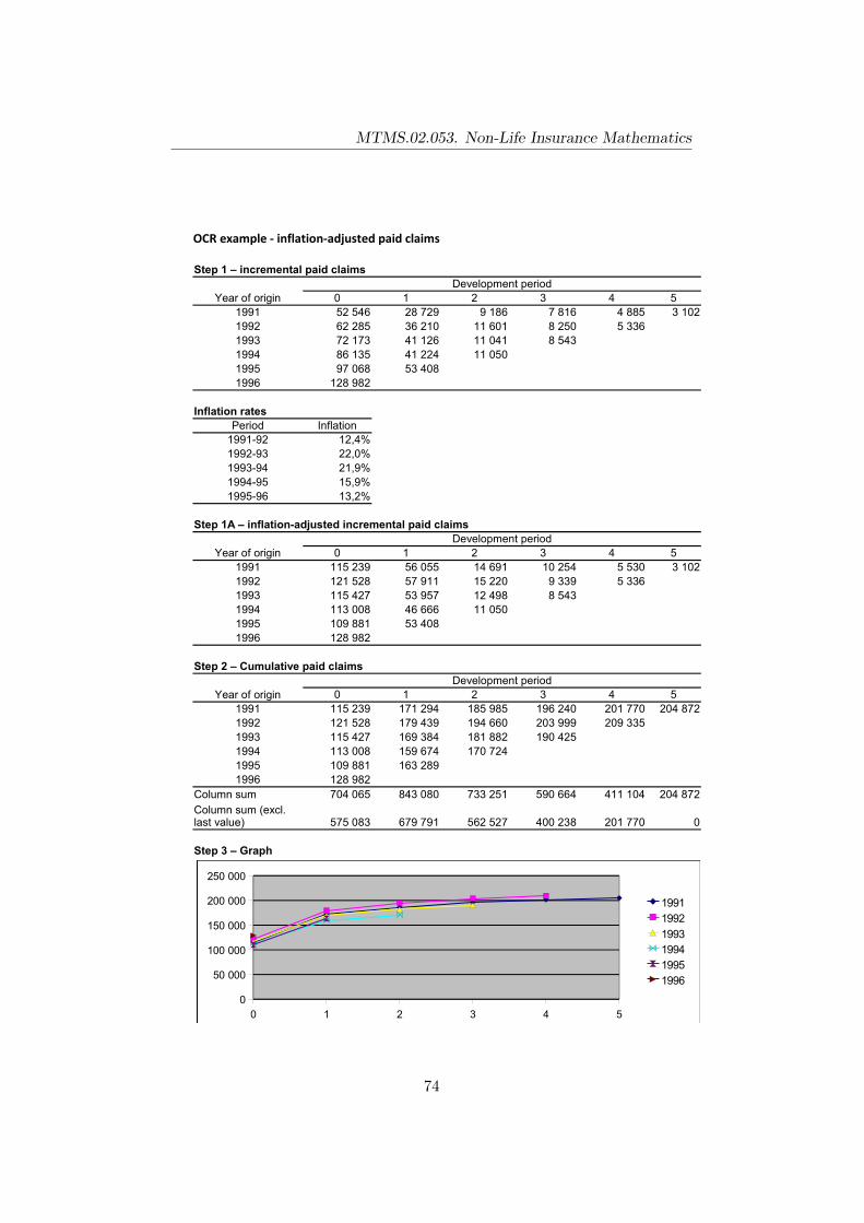
MTMS.02.053. Non-Life Insurance Mathematics
OCR example - inflation-adjusted paid claims
0 1 2 3 4 5199119921993199419951996
1991-92 12,4%1992-93 22,0%1993-94 21,9%1994-95 15,9%1995-96 13,2%
0 1 2 3 4 5199119921993199419951996
0 1 2 3 4 5199119921993199419951996
0
Step 1 – incremental paid claimsDevelopment period
Year of origin52 546 28 729 9 186 7 816 4 885 3 10262 285 36 210 11 601 8 250 5 33672 173 41 126 11 041 8 54386 135 41 224 11 05097 068 53 408
128 982
Inflation ratesPeriod Inflation
Step 1A – inflation-adjusted incremental paid claimsDevelopment period
Year of origin115 239 56 055 14 691 10 254 5 530 3 102121 528 57 911 15 220 9 339 5 336115 427 53 957 12 498 8 543113 008 46 666 11 050109 881 53 408128 982
Step 2 – Cumulative paid claimsDevelopment period
Year of origin115 239 171 294 185 985 196 240 201 770 204 872121 528 179 439 194 660 203 999 209 335115 427 169 384 181 882 190 425113 008 159 674 170 724109 881 163 289128 982
Column sum 704 065 843 080 733 251 590 664 411 104 204 872Column sum (excl. last value) 575 083 679 791 562 527 400 238 201 770
Step 3 – Graph
0 1 2 3 4 50
50 000
100 000
150 000
200 000
250 000
199119921993199419951996
74

MTMS.02.053. Non-Life Insurance Mathematics
OCR example - inflation-adjusted paid claims
0 - 1 1 - 2 2 - 3 3 - 4 4 - 51991 1,486 1,086 1,055 1,028 1,0151992 1,477 1,085 1,048 1,0261993 1,467 1,074 1,0471994 1,413 1,0691995 1,4861996
0 - 1 1 - 2 2 - 3 3 - 4 4 - 51,466 1,079 1,050 1,027 1,015
1,732 1,181 1,095 1,043 1,0150,577 0,847 0,913 0,959 0,985
0 - 1 1 - 2 2 - 3 3 - 4 4 - 51991 1,486 1,086 1,055 1,028 1,0151992 1,477 1,085 1,048 1,026 1,0151993 1,467 1,074 1,047 1,027 1,0151994 1,413 1,069 1,050 1,027 1,0151995 1,486 1,079 1,050 1,027 1,0151996 1,466 1,079 1,050 1,027 1,015
0 1 2 3 4 5199119921993199419951996
Reserve
19921993199419951996
Step 4 – Ratios of cumulative paiments in successive development periodsDevelopment period
Year of origin
Step 5 – Chain ladder ratiosDevelopment period
Ratio0 – ultimate 1 – ultimate 2 – ultimate 3 – ultimate 4 – ultimate
Cumulative factorInverse
Step 6 – Ratios of cumulative payments (step 4 extended)Development period
Year of origin
Step 7 – Cumulative paid claims in current money (step 2 extended)Development period
Year of origin115 239 171 294 185 985 196 240 201 770 204 872121 528 179 439 194 660 203 999 209 335 212 553115 427 169 384 181 882 190 425 195 595 198 602113 008 159 674 170 724 179 263 184 130 186 960109 881 163 289 176 130 184 940 189 961 192 881128 982 189 089 203 960 214 161 219 975 223 357
Step 8 – Estimated reserve
Year of origin
Current money (1996)
Nominal Net present value
3 218 3 605 3 4008 177 9 562 8 820
16 237 19 646 17 79529 592 37 082 32 96694 375 115 415 103 845
Total 151 600 185 310 166 826
75

MTMS.02.053. Non-Life Insurance Mathematics
OCR example - inflation-adjusted paid claims
0 1 2 3 4 5199119921993199419951996
0 1 2 3 4 5199119921993199419951996
0 1 2 3 4 5199119921993199419951996
0 1 2 3 4 5199119921993199419951996
1997 1998 1999 2000 2001199119921993199419951996
Step 9 – Estimated ultimate claims at each development periodDevelopment period
Year of origin199 559 202 337 203 673 204 666 204 872 204 872210 450 211 958 213 173 212 758 212 553199 885 200 081 199 180 198 602195 695 188 611 186 960190 280 192 881223 357
Step 10 – Incremental payments (in 1996 money)Development period
Year of origin115 239 56 055 14 691 10 254 5 530 3 102121 528 57 911 15 220 9 339 5 336 3 218115 427 53 957 12 498 8 543 5 170 3 007113 008 46 666 11 050 8 539 4 867 2 831109 881 53 408 12 841 8 810 5 021 2 920128 982 60 107 14 870 10 202 5 814 3 382
Step 10A – Incremental payments (with future inflation 12% per annum)Development period
Year of origin
3 6055 790 3 772
9 564 6 105 3 97714 382 11 051 7 054 4 595
67 320 18 653 14 333 9 149 5 960
Step 10B – Incremental payments (with future inflation 12%, discounted 6% per annum)Development period
Year of origin
3 4005 462 3 357
9 023 5 433 3 33913 568 9 835 5 923 3 640
63 510 16 601 12 034 7 247 4 454
Step 11 – Estimated future payments by calendar year (in 1996 money)Development period
Year of origin Total
3 218 3 2185 170 3 007 8 1778 539 4 867 2 831 16 237
12 841 8 810 5 021 2 920 29 59260 107 14 870 10 202 5 814 3 382 94 375
Total 89 876 31 554 18 053 8 735 3 382 151 600
76

MTMS.02.053. Non-Life Insurance Mathematics
OCR example - inflation-adjusted paid claims
0 1 2 3 4 5199119921993199419951996
0 1 2 3 4 51991 922 897 197 01992 711 -369 -1971993 741 511 -724 -528199419951996 0
Step 12 – Back-fitted incremental claimsDevelopment period
Year of origin118 307 55 133 13 640 9 357 5 333 3 102122 743 57 200 14 151 9 708 5 533114 687 53 446 13 222 9 071107 964 50 313 12 447111 383 51 906128 982
Step 13 – Residuals (actual – expected)Development period
Year of origin-3 068 1 052-1 215 1 069
5 044 -3 647 -1 397-1 502 1 502
77

MTMS.02.053. Non-Life Insurance Mathematics
11.2.2 Loss ratio and Bornhutter-Ferguson method
Besides using only claim-based data for reserve estimation it is also pos-sible to take into account the (relevant) premiums. A simplest calculationof reserves could be made by multiplying premiums by the expected lossratio (obviously the true loss ratio is not yet known) to get an estimate forultimate claim amount.
Example 11.2. Assume that the expected loss ratio is 0.8 and after devel-opment period j the loss ratio based on known claims is 0.71. Then one canestimate that the remaining IBNR reserve at the end of period j should beabout 0.8− 0.71 = 0.09, i.e. 9% of premiums.
The Bornhutter-Ferguson method gives a way of combining the prior expec-tation of losses provided by simple loss ratio estimates with the actual rateof emergence of claims. The estimated ultimate claims for year of origin i atthe end of developent period j (i.e. using the information available at theend of development period j) is given by
Si = Pi · IELRi(1−Rj) + Cij ,
where
• Pi is the premium income received;
• IELRi is the initial expected loss ratio for year of origin i;
• Rj is the proportion factor at the end of the on jth development period;
• Cij is the (cumulative) amount of claims for year of origin i and de-velopment year j.
11.2.3 Chain ladder as a generalized linear model
The methods considered so far are mainly based on averages and do notprovide only point estimates. The other weak point is that there is no way tomeasure the goodnes of fit of proposed models. In the following we considercertain stochastic reserve estimation methods that also allow us to estimatethe variability of predicted claims reserves.
Firstly, we note that several often used and traditional actuarial methods tocomplete a run-off triangle can be described by one generalized linear model(GLM). Let the random variables Cij , i = 0, 1, . . . , I and j = 0, 1, . . . , Jdenote the random variables corresponding to the claim figure for year oforigin i and year of development j, as previously. We consider the followingmultiplicative model
Cij ≈ αi · βj · γk, (11.1)
78

MTMS.02.053. Non-Life Insurance Mathematics
where αi is the parameter that describes the effect of year of origin i, βj isthe parameter corresponding to development year j, and γk describes theeffect of calendar year k = i+ j.
The expected value of Cij can be given as
ECij = exp{lnαi + lnβj + ln γk},
or, equivalently,lnECij = lnαi + lnβj + ln γk,
so there is a logarithmic link function (or log-link).
Turns out that this simple model allows generate quite a few reserving tech-niques, depending on the assuptions set on distribution of the Cij .
If we restrict the model (11.1) to
Cij ∼ Po(αiβj), γk ≡ 1, (11.2)
where Cij are independent for different i, j = 1, . . . , I; i + j ≤ I, then weobtain the chain ladder method. Indeed, if the parameters αi > 0 and βj areto be estimated by maximum likelihood, then model (11.2) is a multiplicativeGLM with log-link. Also the (Poisson) distributional assumption allows tofind estimates for other characteristics of the predicted claims reserves, suchas variance.
It can be shown that the optimal parameters αi and βj produced by thisGLM are equal to the optimal estimates obtained by the chain laddermethod.
11.2.4 Mack’s stochastic model behind the chain ladder
In the previous subsection we saw that the chain ladder method can beconsidered as an algorithm to estimate the parameters of a simple GLMwith two factors (year of origin and development year). In 1993 ThomasMack describes ’the’ stochastic model behind chain ladder as a differentset of assumptions under which doing these calculations makes sense. Asthe proposed model is distribution-free, the maximum likelihood approachcannot be used, instead certain unbiased linear estimators for the meansquared errors are found. Let us recall that the mean squared error (MSE)of an estimate is the variance of the estimate plus the square of its bias.Therefore, if an estimate is unbiased, its MSE is equal to its variance, whichmakes MSE a convenient choice to model the variability of the predictions.
The Mack’s model for chain ladder is described by three assumptions:
79
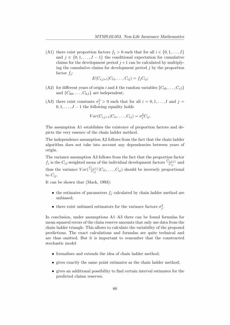
MTMS.02.053. Non-Life Insurance Mathematics
(A1) there exist proportion factors fj > 0 such that for all i ∈ {0, 1, . . . , I}and j ∈ {0, 1, . . . , J − 1} the conditional expectation for cumulativeclaims for the development period j+1 can be calculated by multiply-ing the cumulative claims for development period j by the proportionfactor fj :
E(Ci,j+1|Ci1, . . . , Cij) = fjCij ;
(A2) for different years of origin i and k the random variables {Ci0, . . . , CiJ}and {Ck0, . . . , CkJ} are independent;
(A3) there exist constants σ2j > 0 such that for all i = 0, 1, . . . , I and j =
0, 1, . . . , J − 1 the following equality holds
V ar(Ci,j+1|Ci1, . . . , Cij) = σ2jCij .
The assumption A1 establishes the existence of proportion factors and de-picts the very essence of the chain ladder method.
The independence assumption A2 follows from the fact that the chain ladderalgorithm does not take into account any dependencies between years oforigin.
The variance assumption A3 follows from the fact that the proportion factorfj is the Cij-weighted mean of the individual development factors
Ci,j+1
Cijand
thus the variance V ar(Ci,j+1
Cij|Ci1, . . . , Cij) should be inversely proportional
to Cij .
It can be shown that (Mack, 1993):
• the estimates of parameters fj calculated by chain ladder method areunbiased;
• there exist unbiased estimators for the variance factors σ2j .
In conclusion, under assumptions A1–A3 there can be found formulas formean squared errors of the claim reserve amounts that only use data from thechain ladder triangle. This allows to calculate the variability of the proposedpredictions. The exact calculations and formulas are quite technical andare thus omitted. But it is important to remember that the constructedstochastic model
• formalizes and extends the idea of chain ladder method;
• gives exactly the same point estimates as the chain ladder method;
• gives an additional possibility to find certain interval estimates for thepredicted claims reserves.
80

MTMS.02.053. Non-Life Insurance Mathematics
11.2.5 Chain ladder bootstrap
Bootstrapping is a simple and powerful method which enables the calcula-tion of a number of different estimates of a random variable, using empiricaldata as an approximation of the true distribution. In other words, no distri-butional assumptions are made, the only assumption is that available datais representative enough for the underlying population.
In this section we briefly introduce the idea of bootstrap method and showhow it can be applied to calculated errors associated with the predictedclaims reserves.
Let us assume that the chain ladder development factors are found and theultimate claims are estimated. We can now back-fit the claims in the run-off triangle based on the ultimate claims and development factors to obtainthe run-off triangle (say, with components Cij) which follows exactly theproposed model:
Development period jYear of origin i 0 1 2 . . . J
0 C00 C01 C02 . . . C0J
1 C10 C11 . . .
2 C20 . . .. . . . . .
I CI0
Here Cij is calculated from
Cij =Ri
fj · . . . · fJ−1
,
where Ri and fj denote estimated values for ultimate claims for year of origini and proportion factor between development years j and j+1, respectively.
The cumulative back-fitted claims are found as differences between actualand expected values:
Year of Development period jorigin i 0 1 2 . . . J
0 C00 − C00 C01 − C01 C02 − C02 . . . C0J − C0J
1 C10 − C10 C11 − C11 . . .
2 C20 − C20 . . .. . . . . .
I CI0 − CI0
If we now move from cumulative differences to incremental differences to re-move the cumulative effect, we obtain a run-off triangle which consists of the
81

MTMS.02.053. Non-Life Insurance Mathematics
residual errors. The residual errors (or simply residuals) give us informationhow well the model fits to the known data and allows to make predictionsabout the future fit.
We now make assumption that the residual errors are random. This assump-tion should actually be tested to ensure there is no systematic component,but it is consistent with the chain ladder model. The significance of thisassumption for the bootstrap method is that each error could equally wellhave arisen as the residual error from any other development period andyear of origin.
Now we are ready to formulate the chain ladder bootstrap algorithm:
Step 1: fix the number of repetitions n.
Step 2: for each repetition i = 1, . . . , n:
2.1) draw a random sample (allowing for replacement) from the set ofresidual errors (in other words, we produce an alternative set ofequally likely outcomes, called the pseudo data);
2.2) create incremental pseudo claims by adding the pseudo residualsto actual claims;
2.3) cumulate the incremental pseudo claims;
2.4) apply the chain ladder method to cumulative claims as normallyto obtain a reserve estimate.
Step 3: now we have n estimates for the reserves, which, by the assump-tions provide a random sample of the distribution of the true reservevalue. This sample can be used to calculate estimates for differentcharacteristics of the distribution (e.g. variance).
In case the incremental claims are affected by inflation then the data shouldbe adjusted by inflation before applying the bootstrap procedure.
References
1. Booth P., Chadburn, R., Cooper, D., Haberman, S., James, D. (1999)Modern Actuarial Theory and Practice. Chapman & Hall / CRC.
2. Kaas, R., Goovaerts, M., Dhaene, J., Denuit, M. (2008) Modern Actu-arial Risk Theory: Using R. Springer, Berlin/Heidelberg.
3. Mack, T. (1993) Distribution-free Calculation of the Standard Errorof Chain Ladder Reserve Estimates. Astin Bulletin, 23, 213–225.
82

MTMS.02.053. Non-Life Insurance Mathematics
12 Using individual history in premium calcula-tion
12.1 Bayesian credibility theory
Let us consider the following motivating problem.
Example 12.1. An insurance company has a long-time customer with av-erage claim amount per year x (e.g., x = 1600). On the other hand, theestimated average claim for similar risks in the insurer’s portfolio is µ (e.g.µ = 2500). How much premium should the insurer ask from this customer?1600? 2500? Or something in between?
To answer this question we need to estimate the credibility of the customer(or customer data), which can be mathematically described by the credibilityfactor z.
Let z = 0.6, then the (pure) premium is found as
P = 0.6 · 1600 + 0.4 · 2500 = 1960.
In general, the premium is found as a weighted average
P = z · x+ (1− z)µ,
where
• x – estimated claim amount (or number) for some fixed risk;
• µ – reference value, expected claim amount (or number) obtained byanalysis of similar risks (collateral information);
• z – credibility factor, 0 ≤ z ≤ 1.
What properties should the credibility factor z have?
It should increase if
• there is more data about the particular risk;
• the precision of individual risks becomes greater.
It should decrease if
• there is more collateral information;
• the collateral risk becomes more relevant.
83

MTMS.02.053. Non-Life Insurance Mathematics
12.1.1 Poisson/gamma model
Suppose that the number of claims in a portfolio is Poisson distributed withparameter λ, where the value of λ is a realization of a gamma distributedrandom variable Λ (Λ ∼ Γ(α, β)). Suppose also that for some risk the claimnumbers in past k years are known: n1, . . . , nk.
The problem is to estimate based on this information (prior distribution andhistory) the (conditional!) expected claim number for the next year:
E(E(N |Λ)|n1, . . . , nk) = E(Λ|n1, . . . , nk).
Notice that this problem is closely related to the setup of Bayesian statis-tics: we need to estimate the posterior distribution of Λ based on the priordistribution of Λ and the observations n1, . . . , nk.
By Bayes Theorem the distribution of (Λ|n1, . . . , nk) is Γ(α+∑k
i=1 ni, β+k)(check it!).
We are mostly interested in its expectation:
E(Λ|n1, . . . , nk) =α+
∑ki=1 ni
β + k=
β
β + k· αβ
+k
β + k·∑k
i=1 nik
.
Taking z = kβ+k , we can write
E(Λ|n1, . . . , nk) = z
∑ki=1 nkn
+ (1− z)αβ.
Recall that we have initial estimates for the expectation based on twosources:
• µ = αβ (based on Γ(α, β));
• n =∑ki=1 nik (based on individual history).
Then the conditional expectation can be written as
E(Λ|n1, . . . , nk) = z · n+ (1− z)µ,
i.e. it is a weighted average of the initial estimates.
It is easy to see that always 0 ≤ z ≤ 1 and the more history we have thehigher z.
84

MTMS.02.053. Non-Life Insurance Mathematics
12.1.2 Normal/normal model
Suppose that claim sizes X are normally distributed (X ∼ N(θ, σ1)), whereθ is fixed, but unknown (and σ1 is assumed to be known). Let us also haveclaims information for some risk in past k years: x1, . . . , xk.
Supposing now that the collateral information gives prior Θ ∼ N(µ, σ2)distribution for θ, we have the following problem of Bayesian statistics: es-timate the posterior distribution of Θ based on its prior distribution andobservations x1, . . . , xk.
By Bayes Theorem the posterior distribution of Θ is
N
(µσ2
1 + kσ22x
σ21 + kσ2
2
,σ2
1σ22
σ21 + kσ2
2
),
where x =∑ki=1 xik .
Thus, the conditional expectation is
E(E(X|Θ)|x1, . . . , xk) = E(Θ|x1, . . . , xk)
=µσ2
1 + kσ22x
σ21 + kσ2
2
=σ2
1
σ21 + kσ2
2
µ+kσ2
2
σ21 + kσ2
2
x.
Taking
z =kσ2
2
σ21 + kσ2
2
=k
k +σ21
σ22
,
the posterior expectation can be written as a weighted average of priorexpectation µ and the mean value of observed claims x:
E(Θ|x1, . . . , xk) = z · x+ (1− z)µ,
One can see that again always 0 ≤ z ≤ 1 and the more history we have thehigher z.
12.2 Empirical Bayesian credibility theory
In Bayesian credibility models, the information came from two sources: apriori distribution of collateral data describing the between risk informationand the individual history. In empirical Bayesian credibility theory (EBCT),the general idea stays the same, we simply drop the distributional assump-tion set to collateral data and study certain distribution-free models.
85

MTMS.02.053. Non-Life Insurance Mathematics
12.2.1 The Buhlmann credibility model
Let us consider a portfolio with n risks and let Xij , j = 1, . . . , k denotethe (aggregate) claim amounts (or numbers) that arise from risk i for ksuccessive years.
Now, let us consider a similar model to Bayesian credibility model, where thedistributional assumptions are replaced with certain structural assumptions:
• the distribution of each Xij , i = 1, . . . , n, j = 1, . . . , k depends onthe value of an unknown parameter Θi, which is assumed to be an(unknown) random variable, but its value θi is fixed for given risk;
• given θi, the random variables Xij , j = 1, . . . , k are i.i.d.;
• for different risks i and i′ (i 6= i′), the pairs of variables (Θi, Xij) and(Θi′ , Xi′j′), j, j
′ = 1, . . . , k, are i.i.d. This assumption allows us to writesimply Θ instad of Θi, since the distribution of Θi does not depend oni.
• the conditional mean and variance of Xij are
E(Xij |Θi) = µ(Θi) = µ(Θ),
V ar(Xij |Θi) = σ2(Θi) = σ2(Θ).
Now, the unconditional mean and variance for Xij are calculated as
EXij = E(E(Xij |Θ)) = Eµ(Θ),
V arXij = E(V ar(Xij |Θ)) + V ar(E(Xij |Θ)) = Eσ2(Θ) + V ar(µ(Θ)),
where the decomposition of variance is based on the law of total variance.
The variance components can be interpreted as follows:
• Eσ2(Θ) represents the expected value of the process variance, i.e. thevariance within risk ;
• V ar(µ(Θ)) is the variance of the hypothetical means, i.e., the variancebetween the risks.
Now, assume that for past k years the claim amounts (or numbers) xij(the realizations of Xij), j = 1, . . . , k, for risk i are known. Then all thestructural parameters, Eµ(Θ), Eσ2(Θ) and V ar(µ(Θ)) can be estimatedfrom the collateral data. The usual estimators are:
Eµ(Θ) = x =1
n
n∑i=1
xi =1
nk
n∑i=1
k∑j=1
xij ,
86

MTMS.02.053. Non-Life Insurance Mathematics
Eσ2(Θ) =1
n
n∑i=1
1
k − 1
k∑j=1
(xij − xi)2
and
V ar(µ(Θ)) =1
n− 1
n∑i=1
(xi − x)2 − 1
nk
n∑i=1
1
k − 1
k∑j=1
(xij − xi)2.
Thus, we have again two sources of information: the individual history givesus mean value xi = 1
k
∑kj=1 xij and the collateral information suggests over-
all mean x.
Now, the formula for credibility premium for risk i in Buhlmann model canbe written as
Pi = z · xi + (1− z) · x
and the remaining question is how to calculate a proper credibility factor z.
Let us now recall the credibility factor for normal/normal model
z =k
k +σ21
σ22
,
where σ21 and σ2
2 can be interpreted as the within risk variance is the be-tween risk variance, respectively. Turns out that similar property holds forPoisson/gamma model: the credibility factor is given by z = k
k+β or, equiv-alently,
z =k
k + α/βα/β2
where we recognize that
• αβ is the expectation (and hence also the variance) of the Poisson dis-tribution, so it describes the within risk variance;
• αβ2 is the variance of the gamma distribution, i.e. the between riskvariance.
These expressions for credibility factor suggest the following formula for thecredibility factor in empirical setup:
z =k
k + Eσ2(Θ)V ar(µ(Θ))
.
87

MTMS.02.053. Non-Life Insurance Mathematics
Notice that although Eσ2(Θ) and V ar(µ(Θ)) are always positive, the pro-posed estimator for V ar(µ(Θ)) can take negative values, as well. In thatcase, one can just take the corresponding estimate equal to zero, which im-plies the credibility factor z is also equal to zero (basically, this assumptionmeans that there is no between risks variance, so the collateral informationcan be fully trusted). So, the value of credibility factor z will always satisfy0 ≤ z ≤ 1.
In conclusion, in the Buhlmann credibility model
• the credibility factor z is the same for all risks in the collective, it onlyhas to be calculated once;
• the more information concerning individual risk (the bigger k) thebigger is z;
• large values of Eσ2(Θ) correspond to large variability from year toyear within risks and implies smaller value of credibility factor z;
• large values of V ar(µ(Θ)) mean large variability between risks andthus the data from other risks is not very informative or relevant,implying higher credibility factor (i.e. the data from an individual riskis more important).
12.2.2 The Buhlmann-Straub model
We saw that the Buhlmann model provides a convenient way to model a het-erogeneous portfolio. At the same time, the Buhlmann model has a seriouslimitation that the the claim amounts (or numbers) for a risk are identi-cally distributed for all years of exposure. In practice, this assumption isoften violated. This issue is addressed in the Buhlmann-Straub model: theassumption of i.i.d. claims is relaxed by introducing an additional exposureor risk volume parameter.
In particular, let us consider again a portfolio with n risks and k successiveyears. Let Yij denote the aggregate claim amount for risk i in year j andlet us introduce the claim amount per unit of risk volume (or per unit ofexposure)
Xij =Yijvij
,
where vij represents the the risk volume. The risk volumes vij are assumedto be known and fixed for each risk i and year j.
Example 12.2. In practice, several different risk volumes are used, depend-ing on the line of business and risk specifics:
88

MTMS.02.053. Non-Life Insurance Mathematics
• number of years at risk in motor insurance;
• total amount of wages in the collective health or collective accidentinsurance;
• sum insured in fire insurance;
• annual turnover in commercial liability insurance;
• annual premium (written or earned) by the ceding company in excessof loss reinsurance.
Similarly to Buhlmann model, a random variable Xij is assumed to dependfrom a parameter Θi, which is unknown, but its value θi is fixed for eachrisk i .
The general assumptions of the Buhlmann-Straub model are:
• given θi, the random variables Xij , j = 1, . . . , k, are independent;
• E(Xij |Θi) =: µ(Θi) does not depend on j;
• vijV ar(Xij |Θi) =: σ2(Θi) does not depend on j;
• for different risks i and i′ (i 6= i′), the pairs of variables (Θi, Xij) and(Θi′ , Xi′j′), j, j
′ = 1, . . . , k, are i.i.d.;
• the risk parameters Θi, i = 1, . . . , n are i.i.d.
The last assumption allows us to write simply Θ instad of Θi, since thedistribution of Θi does not depend on i.
Then, the credibility premium for risk i can be found as
Pi = zi · xi + (1− zi) · Eµ(Θ),
where the meaning of xi and the calculation of an estimate for Eµ(Θ) areslightly changed compared to Buhlmann model:
xi =
∑kj=1 vijxij∑kj=1 vij
=
∑kj=1 yij∑kj=1 vij
and
Eµ(Θ) = x =
∑ni=1
∑kj=1 vijxij∑n
i=1
∑kj=1 vij
=
∑ni=1
∑kj=1 yij∑n
i=1
∑kj=1 vij
,
where xij and yij are the realizations of Xij and Yij , respectively.
89

MTMS.02.053. Non-Life Insurance Mathematics
Similarly, the estimates for variance components are now adjusted by riskvolume as follows:
Eσ2(Θ) =1
n
n∑i=1
1
k − 1
k∑j=1
vij(xij − xi)2
and
V ar(µ(Θ)) =1
v
1
nk − 1
n∑i=1
k∑j=1
vij(xij − x)2 − 1
n
n∑i=1
1
k − 1
k∑j=1
vij(xij − xi)2
,where
v =1
nk − 1
n∑i=1
k∑j=1
vij
(1−
∑kj=1 vij∑n
i=1
∑kj=1
vij
).
Now, the credibility factor is given by
zi =
∑kj=1 vij∑k
j=1 vij + Eσ2(Θ)V ar(µ(Θ))
.
By similar argumentation as before, we can see that 0 ≤ zi ≤ 1. Also, thegeneral idea underlying this model is the same as in Buhlmann model. Themain difference in the calculation of credibility factor is that the numberof years k is changed to the aggregate risk volume, which is obviously amore informative characteristic. The calculation of estimates for structuralparameters is also slightly changed, but their meaning is the same: Eσ2(Θ)describes the within risk variance and V ar(µ(Θ)) is the between risks vari-ance.
To sum up, we also mention the following:
• in case all the volumes vij are equal to 1, the Buhlmann-Straub modelreverts to the Buhlmann model;
• zi is increasing function of aggregate risk volume for risk i: higher riskvolume implies higher credibility for that risk;
• although we formulated all the results assuming the variables Yij repre-sent claim amounts, the same model can be applied to claim numbers,as well;
• the Buhlmann-Straub model is by far the most used credibility modelin insurance practice.
90

MTMS.02.053. Non-Life Insurance Mathematics
12.3 Bonus-malus systems (No Claims Discount systems)
We consider the following situation
• insurer has sufficient history of its customers’ (policyholders’) claimbehaviour;
• insurer is interested in keeping its ”good” customers (who cause no orfew claims);
• insurer is willing to offer certain discount to keep the good customers.
The main question we search answers for is how to construct a suitablediscount system.
Example 12.3 (A three-level NCD system). Let us consider the followingsimple system:
level discount
0 0%
1 25%
2 40%
The rules how a policyholder can reach different discount levels will be spec-ified later on.
In general, let us have n discount levels (categories) and let πi denote theproportion of policyholders at i-th level (
∑i πi = 1). To give a formal de-
scription of an NCD system we need to recall some properties and resultsrelated to Markov chains.
Let us denote~π = (π0, π1, . . . , πn)
and
P = (pij) =
p00 p01 . . . p0n
p10 p11 . . . p1n...
.... . .
...pn0 pn1 . . . pnn
,
where pij are transition probabilities, i.e. probabilities that (based on theclaim behaviour of the next year) a policyholder will move from discountlevel i to discount level j. Matrix P is called the transition matrix.
An important task for insurer is to estimate the vector ~π. In case there existsa steady state, i.e. ~π = ~π · P , we can find ~π by solving the correspondingsystem of equations.
Example 12.4. Let us now extend the NCD system described in previousexample by the following rules:
91

MTMS.02.053. Non-Life Insurance Mathematics
• in case of a claim-free year the policyholder moves in the next year tothe next higher level of discount (if possible);
• in case of claim(s) the policyholder moves in the next year to nextlower level of discount (if possible).
Let the probability of a loss be 0.1. The corresponding transition matrix is:
P =
0.1 0.9 00.1 0 0.90 0.1 0.9
and ~π = ~π · P gives
0.1π0 + 0.1π1 = π0
0.9π0 + 0.1π2 = π1
0.9π1 + 0.9π2 = π2
π0 + π1 + π2 = 1
,
which has solution π0 = 191 , π1 = 9
91 ja π2 = 8191 .
In practice the assumption that all customers have the same loss probabilityis obviously oversimplified. Still, the customers can be divided by their claimbehaviour into ”good” and ”bad” categories and the loss probability can beestimated in those categories separately.
Let us extend the example even further Let the probability of ”good” drivershaving an accident be 0.1 and for ”bad” drivers 0.2. Then the steady statedistribution for ”good” drivers is given in previous example and for ”bad”drivers the proportions are (check it!): π0 = 1
21 , π1 = 421 and π2 = 16
21 .
Suppose that the full (individual) premium c. Then the average pure pre-mium paid by a ”good” driver is
1
91c+
9
91· 0.75c+
81
91· 0.6c = 0.619c
and the average pure premium paid by a ”bad” driver is
1
21c+
4
21· 0.75c+
16
21· 0.6c = 0.648c.
Thus, in spite the fact that ”bad” drivers are twice as likely to claim as”good” drivers, the premium they pay is only marginally higher (on average).
The following example shows how a discount system may affect the policy-holders decision whether to make the claim. In other words, the probabilitythat there incurs a loss is not the same as the probability that a clame ismade!
92

MTMS.02.053. Non-Life Insurance Mathematics
Example 12.5. Consider the same 3-level discount system (0%, 25% ja40%), where policyholders move between discount levels as specified in pre-vious examples. Let the policyholders be divided into two groups: ”good”drivers and ”bad” drivers with accident probabilities 0.1 and 0.2, respec-tively. The probability of any driver having two or more accidents is sosmall it may be assumed to be zero. The cost of repair following an accidenthas lognormal distribution with parameters µ = 5 and σ = 2 (in EUR). Theannual premium for policyholders (without discount) is 500 EUR. A policy-holder makes a claim following an accident only if the cost of the repair isgreater than the win from the discounts of premium in the following threeyears in case no claim is made.
For each level of discount, calculate
(a) the cost of repair below which a policyholder will not claim;
(b) the probability that a policyholder will make a claim following anaccident;
(c) the proportions of ”good” and ”bad” drivers assuming these propor-tions have reached a steady state.
(a) A policyholder will decide whether to make a claim following an accidentcomparing the sums the premiums payable in the next three years
(i) given that a claim is made for the cost of repair (and assuming noclaims in the following years);
(ii) given that no claim is made for the cost of this repair (and assumingno claims in the following years).
A policyholder will make a claim only if the cost of repair is greater thandifference between (i) and (ii), i.e.
• for discount level 0%: (500 + 375 + 300)− (375 + 300 + 300) = 200;
• for discount level 25%: (500 + 375 + 300)− (300 + 300 + 300) = 275;
• for discount level 40%: (375 + 300 + 300)− (300 + 300 + 300) = 75.
(b) Let X denote the loss size, then lnX ∼ N(5, 2). The claim will only bemade if it exceed certain threshold x, i.e.
P{X > x} = P{lnX > lnx} = 1− Φ
(lnx− 5
2
).
The threshold x is different for each level of discount and found in (a).
Thus the claim probabilities in case of accident are:
93

MTMS.02.053. Non-Life Insurance Mathematics
• for discount level 0%: 1− Φ(
ln 200−52
)= 1− Φ(0.149) = 0.441;
• for discount level 25%: 1− Φ(
ln 275−52
)= 1− Φ(0.308) = 0.379;
• for discount level 40%: 1− Φ(
ln 75−52
)= 1− Φ(−0.341) = 0.633.
(c) Let us consider ”good” and ”bad” drivers separately. Since
P{claim} = P{claim|accident} ·P{accident},
the transition matrix for ”good” drivers is
P =
0.0441 0.9559 00.0379 0 0.9621
0 0.0633 0.9367
.
At the steady state we obtain the following system of equations0.0441π0 + 0.0379π1 = π0
0.9559π0 + 0.0633π2 = π1
0.9621π1 + 0.9367π2 = π2
π0 + π1 + π2 = 1
,
which has solution (check it!) π0 = 0.0024, π1 = 0.0616 ja π2 = 0.9360.
The transition matrix for ”bad” drivers is
P =
0.0882 0.9118 00.0758 0 0.9242
0 0.1266 0.8734
and the solution of steady state system gives
• π0 = 0.0099,
• π1 = 0.1193,
• π2 = 0.8708.
References
1. Booth P., Chadburn, R., Cooper, D., Haberman, S., James, D. (1999)Modern Actuarial Theory and Practice. Chapman & Hall / CRC.
2. Buhlmann, H., Gisler, A. (2005) A Course in Credibility Theory andits Applications. Springer, Berlin/Heidelberg.
94

MTMS.02.053. Non-Life Insurance Mathematics
3. Gray, R.J. & Pitts, S.M. (2012) Risk Modelling in General Insurance.From Principles to Practice. Cambridge University Press.
4. Casualty Actuarial Society. (1998) Foundations of Casualty ActuarialScience. Casualty Actuarial Society.
5. Hossack, I.B., Pollard, J.H., Zehnwirth, B. (1995) Introductory Statis-tics with Applications in General Insurance. Cambridge UniversityPress.
6. Kaas, R., Goovaerts, M., Dhaene, J., Denuit, M. (2008) Modern Actu-arial Risk Theory: Using R. Springer, Berlin/Heidelberg.
7. Tse, Y.-K. (2009) Nonlife Actuarial Models. Cambridge UniversityPress.
95

MTMS.02.053. Non-Life Insurance Mathematics
13 The accounting framework
To understand the operation of a company it is important that the contentof the accounts and the relationship between revenue accounts and balancesheets is clearly understood.
A brief description of key terms follows:
• the revenue account summarizes the cash flows incurred during theyear due to the insurance business;
• the profit and loss account incorporates the insurance result from rev-enue account, as well as other cash flows (e.g. tax and dividend pay-ments, investments, etc);
• the balance sheet provides a view of the total assets and the liabilitiesof the company at one moment in time.
The revenue and profit and loss accounts therefore provide the link betweenthe opening (or brought forward) balance sheet and the closing (or carriedforward) balance sheet.
The following figure demonstrates the connection between the various partsof the accounts and certain cash flows.
96

MTMS.02.053. Non-Life Insurance Mathematics
13.1 The revenue account
The amount of premium included in the accounts is the earned premium.Recall that using the unearned premiums reserve (UPR), the total premiumearned in an accounting year is found as:
UPR brought forward from the previous accounting year
+ the premium written in the accounting year
− the UPR carried forward to the next accounting year.
Similary, the insurer must account for the claims incurred during the year,not for the claims paid during the accounting year. Thus, using the out-standing claims reserve (OCR), the claims incurred are calculated as:
the claims paid
− outstanding claims reserves brought forward
+ outstanding claims reserves carried forward.
The items above, together with expenses associated with underwriting ac-tivities and commission, are combined in the revenue account to producethe underwriting result as follows:
earned premium
− incurred claims
− expenses and commission.
13.2 The profit and loss account
The profit and loss account is a continuation of the revenue account, reflect-ing those revenues and expenses not directly attributable to the underwritingactivities.
A typical profit and loss account of a non-life insurance company includesthe following items:
+ balance of profit and loss account brought forward
+ investment income
+ capital gains
− overhead expenses
+ exceptional items
97

MTMS.02.053. Non-Life Insurance Mathematics
+ underwriting profit
= overall result
− tax liability
− dividend payments
= balance of profit and loss account carried forward
13.3 The balance sheet
The balance sheet gives a view of the financial position of the company.It is divided into two parts describing different aspects of the company’sbusiness:
• assets;
• liabilities and equity.
For a non-life insurance company, these parts are likely to include the fol-lowing components.
Assets
• Investments
– Equity
– Fixed interest
– Property
• Current assets
– Debtors
– Cash
Total assets
Liabilities and equity
• Liabilities
– Technical reserves
∗ OCR carried forward
∗ IBNR carried forward
∗ UPR carried forward
98
MTMS.02.053. Non-Life Insurance Mathematics
∗ DAC carried forward
∗ URR carried forward
– Other contingency reserves carried forward
– Creditors
– Long-term liabilities (loans, etc)
• Equity
– Share capital
– Retained earnings
Total liabilities + Equity
13.4 Key analytical statistics
Accounts can only provide summary information. They are particularly de-ficient in indicating the inherent uncertainty in both the amount and timingof asset receipts and liability outgo. This is a fundamental issue in insuranceand to improve the presentation of information (e.g. for a supervisory per-spective), certain financial characteristics of different insurers can be com-pared, and the performance of individual companies can be tracked throughtime. This includes characteristics related to premium growth, changes inthe asset portfolio or in the solvency, and more:
• premium growth statistics, e.g.
premium written in year t
premium written in year t− 1
or
premium written in year t− premium written in year t− 1
premium written in year t− 1;
• net income growth
net income in year t− net income in year t− 1
net income in year t− 1;
• reinsurance related ratios
net written premium
gross written premium;
net paid claims
gross paid claims;
99

MTMS.02.053. Non-Life Insurance Mathematics
net incurred claims
gross incurred claims;
reinsurance debtors
reinsurance recoveries due on paid claims;
• the loss ratioincurred claims
earned premiums;
• the expense ratio
expenses and commission
written premiums;
• the operating ratio
loss ratio + expense ratio;
• the investment ratioinvestment returns
written premiums;
• solvency ratiofree assets
net written premiums.
We also mention some general ratios that are widely used in accountingframework (and are not limited to insurance business only):
• return on assets (ROA)net income
total assets.
• return on equity (ROE)
net income
shareholder’s equity;
• current ratiocurrent assets
current liabilities.
100

MTMS.02.053. Non-Life Insurance Mathematics
13.5 A note on terminology. Premiums
Throughout this section (and the whole course) the term ”premium” is usedin different contexts having slightly different meaning. In the following webriefly recall the used terms for premiums in different situations.
1. (Under)written premium:
• the premium charged (or to be charged) for a policy or group ofpolicies;
• fixed (usually) while signing the contract;
• related date – starting date of the contract.
2. Earned premium
• the premium recognized as revenue for the period in question;
• requires implicit or explicit statement of the corresponding blockof time.
3. Accounted premium
• takes into account sent out invoices;
• describes the premium volume of a portfolio without specifyingthe period when the contracts are signed;
• related date – date when the invoice is issued.
4. Received premium
• actual payments received on insurance company’s bank account;
• related to cash-flow;
• related date – payment date.
In case of reinsurance, we may also categorize premiums as follows.
• Direct premiums – premiums arising from policies covering the cus-tomer’s risks, other than risks from the customer’s insurance/reinsuranceor retrocession policies when the customer is an insurer (or reinsurer).
• Reinsurance premiums – premiums arising from policies coveringrisks from direct insurance policies;
• Retrocession premiums – premiums arising from policies coveringrisks from reinsurance policies.
101

MTMS.02.053. Non-Life Insurance Mathematics
References
1. Booth P., Chadburn, R., Cooper, D., Haberman, S., James, D. (1999)Modern Actuarial Theory and Practice. Chapman & Hall / CRC.
102

MTMS.02.053. Non-Life Insurance Mathematics
14 Solvency II
14.1 Background. Goals. Requirements
In general terms, solvency is the state of having more assets than liabilities.To be solvent means that one is in the state of solvency.
Currently (as of 2013), the regulations in insurance market are specified inthe Solvency I directive, which was introduced already in 1973. The economyand risk management systems are changed a lot during last years, thus theSolvency I regime is outdated in many ways (it is static, volume-based, hasso-called accounting view and does not take risk behaviour and economicfactors into account). Therefore, in order to regulate the insurance marketmore effectively and to enhance the customer protection, a new dynamicregulation Solvency II is proposed and developed. Solvency II has so-calledeconomic view, takes into account the current risk management strategiesand allows much more dynamic capital allocation. Also, since the require-ments specified in Solvency I proved to be not sufficient in many cases,several EU member states have already reformed their insurance regula-tions. Thus, the Solvency II regime also serves as unification of the solvencyregulatory system. The Solvency II regime is expected to go live in January1, 2014.
The specifications for Solvency II regime are obtained through a series ofquantitative impact studies (QIS). Each following study refines the results ofthe previous study and provides more detailed and specific documentationrequired to adapt the Solvency II regime. In total, five quantitative impactstudies were conducted, shortly referred to as QIS1 – QIS5.
The Solvency II framework is divided into three main areas (called pillars,similarly to the known banking supervisory system, Basel II)
• Pillar I (financial pillar): quantitative requirements;
• Pillar II (governance pillar): qualitative requirements – the supervisoryreview process;
• Pillar III (market conduct): statutory and market reporting.
The first pillar includes the calculation of the capital requirements (eitheraccording to standard formula or internal model, more details in next sub-sections). It also includes rules on provisioning and eligible capital.
The second pillar focuses on the supervisors and their review process (e.g., acompany’s internal control and risk management and the approval of usinginternal models in Pillar I).
103
MTMS.02.053. Non-Life Insurance Mathematics
The third pillar includes reporting to both the supervisor and the market.Reporting to market is required to promote market discipline and trans-parency.
The International Association of Insurance Supervisors (IAIS) gives 15 re-quirements for a solvency regime in relation to regulatory capital require-ments:
1. A total balance sheet approach should be used in the assessment ofsolvency to recognize the interdependence between assets, liabilities,regulatory capital requirements and capital resources and to ensurethat risks are appropriately recognized.
2. Regulatory capital requirements should be established at a level suchthat the amount of capital that an insurer is required to hold shouldbe sufficient to ensure that, in adversity, an insurer’s obligations topolicyholders will continue to be met as they fall due.
3. The solvency regime should include a range of solvency control levelswhich trigger different degrees of intervention by the supervisor withand appropriate degree of urgency.
4. The solvency regime should ensure coherence between the solvencycontrol levels established and the associated corrective action that maybe at the disposal of the insurer and/or the supervisor. Correctiveaction may include options to reduce the risks being taken by theinsurer as well as to raise more capital.
5. The regulatory capital requirements in a solvency regime should es-tablish a solvency control level which defines the level above which thesupervisor would not require action to increase the capital resourcesheld or reduce the risks undertaken by the insurer. This is referredto as the solvency capital requirement (SCR) or prescribed capital re-quirement (PCR).
6. The SCR should be defined such that assets will exceed technicalprovisions and other liabilities with a specified level of safety over adefined time horizon.
7. The regulatory capital requirements in a solvency regime should estab-lish a solvency control level which defines the supervisory interventionpoint at which the supervisor would invoke its strongest actions, if fur-ther capital is not made available. This is referred to as the minimumcapital requirement (MCR).
8. The solvency regime should establish a minimum bound on the MCRbelow which no insurer is regarded to be viable to operate effectively.
104
MTMS.02.053. Non-Life Insurance Mathematics
9. The solvency regime should be open and transparent as to the reg-ulatory capital requirements that apply. It should be explicit aboutthe objectives of the regulatory capital requirements and the bases onwhich they are determined.
10. In determining regulatory capital requirements, the solvency regimeshould allow a set of standardized and, if appropriate, other approvedmore tailored approaches such as the use of (partial and full) internalmodels.
11. The solvency regime should be explicit as to where risks are addressed,whether solely in technical provisions, solely in regulatory capital re-quirements or if split between the two, the extent to which the risksare addressed in each. The regime should be explicit as to how risksand their aggregation are reflected in regulatory capital requirements.
12. The supervisor should set out appropriate target criteria for the cal-culation of regulatory capital requirements, which should underlie thecalibration of a standardized approach.
13. Where the supervisory regime allows the use of approved more tailoredapproaches such as internal models for the purpose of determining reg-ulatory capital requirements, the target criteria should also be used bythose approaches for that purpose to ensure broad consistency amongall insurers within the regime.
14. The solvency regime should be designed so that any variations to theregulatory capital requirement imposed by the supervisor are madewithin a transparent framework, are proportionate according to thetarget criteria and are only expected to be required in limited circum-stances.
15. The solvency regime should be supported by appropriate public dis-closure and additional confidential reporting to the supervisor.
To model the solvency capital requirement (SCR), the International Actu-arial Association (IAA) has proposed five main risk categories:
1. insurance risk (or underwriting risk);
2. credit risk;
3. market risk;
4. operational risk;
5. liquidity risk.
105

MTMS.02.053. Non-Life Insurance Mathematics
The underwriting risk refers to the risk related to the businesses that willbe written during the following year. In general, it is considered net of rein-surance, as the reinsurance risk will be dealt with in the default credit riskcategory. The underwriting process risk will thus be highly correlated withthe credit risk.
Credit risk is the risk of not receiving promised payments (e.g., in company’sinvestment portfolio, or reinsurance payments).
Market risk is introduced into an insurer’s operations through variations infinancial markets that cause changes in asset values, products, and portfoliovaluation. Market risks relate to the volatility of the market values of assetsand liabilities due to future changes in asset prices.
Operational risk is the risk of loss resulting from inadequate or failed internalprocesses, people, systems, or from external events. The most common risksthat one may classify under operational risk are the failure in control andmanagement, the failure in IT processes, human errors, fraud, jurisdictionaland legal risks.
Liquidity risk is the risk that an insurer, although solvent, has insufficientliquid assets to meet his obligations (e.g. claim payments) when they falldue.
In the following we mostly concentrate on the problems related to the un-derwriting risk, keeping in mind that that the whole picture is more complexand includes other risk categories.
Generic risks related to underwriting that apply to most lines of businessare:
• underwriting process risk – risk from exposure to financial losses re-lated to the selection and approval of risks to be insured;
• pricing risk – risk that the prices charged by the company for insurancecontracts will be ultimately inadequate;
• product design risk – risk that the company faces risk exposure underits insurance contracts that was unanticipated in the design and pricingof the insurance contract;
• claims risk (for each peril) – risk that many more claims occur than ex-pected, or that some claims that occur are much larger than expected,resulting in unexpected losses;
• economic environment risk – risk that social conditions will change ina manner that has an adverse effect on the company;
106

MTMS.02.053. Non-Life Insurance Mathematics
• net retention risk – risk that higher retention of insurance loss ex-posures results in losses due to catastrophic or concentrated claimsexperience;
• policyholder behaviour risk – risk that the insurance company’s poli-cyholders will act in ways that are unanticipated and have an adverseeffect on the company;
• reserving risk – risk that the provisions held in the insurer’s financialstatements for its policyholder obligations will prove to be inadequate.
In constructing solvency capital requirements (SCR), the following funda-mental issues need to be discussed:
• valuation of assets and liabilities – the economic total balance sheetapproach, i.e. assets and liabilities should be valued in a market-consistent way and their interactions should be a part of the solvencyassessment;
• risk margins for uncertainty in assets and liabilities;
• risk measures for the volatility in assets and liabilities;
• modelling (risk categories, mitigation, diversification, etc).
14.2 Capital requirements in Solvency I
Before going to actual calculation in Solvency II, let us recall how the re-quired capital is found under Solvency I regime.
Recall that in solvency I regime there are two important characteristics thatspecify when the regulatory authorities should take action:
• required (adequate) solvency margin;
• minimum guarantee fund.
In case the solvency margin of an insurance company falls below the requiredmargin, supervisory organizations intervene and require certain actions torestore the adequate solvency margin. The solvency margin should never fallbelow a minimum guarantee fund, which is the absolute minimum amountof capital required.
The current required solvency margin for non-life insurance companies inEU is defined as the maximum of claim based and premium based indexes:
Umin = max(P ∗, S∗).
107

MTMS.02.053. Non-Life Insurance Mathematics
The claims and premium indices are defined as:
P ∗ =
{0.18 · P ·RRe, for P ≤ 50 · 106,
[0.18 · 50 · 106 + 0.16 · (P − 50 · 106)] ·RRe, for P > 50 · 106
and
S∗ =
{0.26 · S ·RRe, for S ≤ 35 · 106,
[0.26 · 35 · 106 + 0.23 · (S − 35 · 106)] ·RRe, for S > 35 · 106,
where P is the annual premium written, S is the average annual amount ofclaims and RRe is the reinsurance ratio.
In other words, the calculation of required solvency margin is simple andstraightforward, it is calculated as maximum of:
• 18% of premium written up to e 50m plus 16% of premiums abovee 50m (adjusted by reinsurance);
• 26% of claims up to e 35m plus 23% of claims above e 35m (adjustedby reinsurance).
The minimum guarantee fund (MGF) is defined as
Umgf = max(v,1
3Umin),
where the margin v is between e 2m and e 3m, depending on the risk class.
Remark 14.1. All the limits in these calculations (e 50m, e 35m, e 2mand e 3m) are revised from time to time and are a subject to change.
14.3 Solvency II standard formula for non-life insurance
The calculation of capital requirements in Solvency II framework can bedone in two ways:
• standard formula – a ready to use system with predetermined correla-tions between risks classes, volatilities, etc; this approach is especiallyconvenient in the transition phase and also more suitable for smallerand medium companies;
• internal model – each insurance company can also develop its ownmodel which will reflect better its individual risk profile.
108

MTMS.02.053. Non-Life Insurance Mathematics
14.3.1 Calculation of the solvency capital requirement SCR
Although with several predetermined relations and margins, the Solvency IIstandard formula framework is still very modular and dynamic (especiallycompared to Solvency I). The general idea of finding SCR consists of findingestimates for SCR in all modules at lower level of aggregation and thenaggregating the results in order to get a higher level estimate. At the verytop level, an insurance company is divided into parts depending on thecompany’s profile (non-life, life, health, etc) and the aggregation rules arespecified. In the next level, each part of the company is also divided intoclasses or modules of risks, then the solvency requirements are found forthese classes and aggregated in order to obtain a requirement correspondingto higher level. Similar approach is applied in all levels of aggregation.
The SCR should be determined as
SCR = BSCR+ CROR −Adj,
where BSCR is the basic SCR, CROR is the capital charge for operationalrisk, and Adj is an adjustment for the risk-absorbing effect of future profitsharing and deferred taxes.
BSCR is SCR before any adjustments, combining capital requirements forfive major risk categories:
• CRNL – the non-life underwriting risk module;
• CRLR – the life underwriting risk module;
• CRHR – the health underwriting risk module;
• CRCR – the credit risk module;
• CRIAR – the intangible assets risk module (intangible asset is an asset,other than a financial asset, that lacks physical substance).
BSCR is found as
BSCR = CRIAR +
√∑i,j
ρij · CRi · CRj ,
where the i and j range over the values given in the list of categories above(NL, LR, HR, CR).
The dependence structure between these risks is assumed to be fixed andknown, the values for ρij are given in the standard formula documentation.
109

MTMS.02.053. Non-Life Insurance Mathematics
Remark 14.2. In many cases linear correlation is not an appropriate choiceto describe the dependency (consider, e.g., skewed distributions, tail depen-dency). In such cases, the correlation parameters should be chosen in sucha way as to achieve the best approximation of the value at risk (V aR) at0.995 for the aggregated capital requirement1. In other words, there is a 1 in200 chance that the insurer’s surplus falls below the margin, so the capitallevel is intended to be such that the insurer could withstand a 1 in 200 yearsshock with sufficient assets remaining.
Let us now focus on the non-life insurance module and corresponding capitalrequirement CRNL.
In the standard formula, there are two risk (sub)modules under the non-lifeunderwriting risk module
• premium and reserve risk submodule;
• catastrophe risk (CAT risk) submodule.
Let the corresponding capital requirements be denoted as CRNL,RP for pre-mium and reserve risk and CRNL,CAT .
It is also assumed that the dependence between these risks ρRP,CAT is 0.25.Conceptually, premium and reserve risks and the catastrophe risk should beindependent, but a positive correlation factor may be appropriate in somesituations, e.g., if underlying distributions are skewed and truncated. Then
Now, the capital requirement for the combined premium and reserve risksis determined as
CRNL,RP = ρ0.995(σRP ) · VRP ,
where VRP is a volume measure (or, more precisely, a combination of volumemeasures from reserve and premium volumes), σRP is combined standarddeviation, and ρ is a charge function, defined by
ρ1−α(σ) =exp
(Φ−1(1− α) ·
√ln(1 + σ2)
)√
1 + σ2− 1.
In other words, the charge function ρ (with α = 0.005) is chosen such that,assuming a lognormal distribution of the underlying risk, a capital charge
1Value at risk (V aR) for random variable X (with continuous and strictly increasingdistribution function F ) at given confidence level α ∈ (0, 1) is defined as
V aR(α) = F−1(α).
110

MTMS.02.053. Non-Life Insurance Mathematics
consistent with the value at risk at 0.995 confidence is produced. Using thelognormal assumption, the charge function is approximately ρ0.995(σ) ≈ 3σ.
The volume measures and standard deviations are calculated for each indi-vidual line of business (LoB) and then aggregated. For each LoB k let usdenote
• VR,k – the volume measure for the reserve risk,
• VP,k – the volume measure for the premium risk,
• VRP,k – the volume measure for the premium and reserve risk,
• σR,k – the volatility measure (standard deviation) for the reserve risk,
• σP,k – the volatility measure (standard deviation) for the premiumrisk,
• σRP,k – the volatility measure (standard deviation) for the premiumand reserve risk.
Then, VR,k is defined as the best estimate for claims outstanding in LoB k.The volume measure for premium risk VR,k is defined as
VP,k = max{Pk(1), P ′k(1), Pk(0)}+Mk,
where Pk(1) is the estimate of the net written premium in the forthcomingyear, P ′k(1) is the estimate of the net earned premium in the forthcomingyear, Pk(0) is the net written premium during the previous year, and Mk isthe expected present value of net claims and expense payments that relate toclaims incurred after the following year and are covered by existing contracts(multiyear contracts).
The volume measure for the premium and reserve risk within each LoB k issimply calculated as the sum of components’ volume measures:
VRP,k = VR,k + VP,k
and the volatility for the reserve and premium risks for each LoB k is cal-culated by
σ2RP,k =
(VR,k · σR,k)2 + (VP,k · σP,k)2 + 2αVR,k · σR,k · VP,k · σP,kV 2RP,k
,
where α is a dependence factor (in QIS4, α is set to 0.5).
All the required values for standard deviations σR,k and σP,k are specifiedin Solvency II documentation (for 12 general LoBs).
111

MTMS.02.053. Non-Life Insurance Mathematics
Now, the overall volume measure is just a sum of volume measures over allLoBs
VRP =∑k
VRP,k
and the overall volatility measure is defined by
σ2RP =
1
V 2RP
∑j,k
ρj,k · Vj · Vk · σj · σk,
where ρj,k denotes the correlation between LoBs j and k and the neededvalues for all combinations of j and k are again specified in Solvency IIdocumentation.
Lastly, without going into details, we also mention that there are two ap-proaches to calculation of required capital in CAT-risk submodule:
• standardized scenario approach – detailed and comprehensive model;
• alternative (factor-based) approach – simplified model, used either indevelopment phase, or in cases that are very clearly specified.
14.3.2 Calculation of the minimum capital requirement MCR
The MCR should ensure a minimum level below the amount of financialresources of an insurer should not fall. In case the resources fall below MCR,the most serious supervisory intervention is triggered.
The MCR is calculated using the following two-step algorithm:
1. Calculate MCRL by
MCRL = MCRNL,NLt +MCRNL,Lt +MCRL,Lt +MCRL,NLt,
where
• MCRNL,NLt denotes the MCR for non-life activities practicedon non-life technical basis,
• MCRNL,NLt denotes the MCR for non-life activities practicedon life technical basis,
• MCRL,Lt denotes the MCR for life activities practiced on lifetechnical basis, and
• MCRL,NLt denotes the MCR for supplementary obligations forlife activities practiced on non-life technical basis.
112

MTMS.02.053. Non-Life Insurance Mathematics
All the components are calculated using the corresponding technicalprovisions and certain weight parameters provided by Solvency II doc-umentation.
2. Squeeze the MCRL into a corridor if needed: MCRL should fit be-tween MCRFloor = 0.25 · SCR and MCRCap = 0.45 · SCR.
Also, MCR must always be higher than an absolute floor AMCR:
MCR = max{MCRL, AMCR},
where the values for AMCR depend on company’s profile and are specifiedin the Solvency II documentation.
References
1. Sandstrom, A. (2010) Handbook of Solvency for Actuaries and RiskManagers: Theory and Practice. Taylor & Francis.
113

MTMS.02.053. Non-Life Insurance Mathematics
List of references
1. Booth P., Chadburn, R., Cooper, D., Haberman, S., James, D. (1999)Modern Actuarial Theory and Practice. Chapman & Hall / CRC.
2. Buhlmann, H., Gisler, A. (2005) A Course in Credibility Theory andits Applications. Springer, Berlin/Heidelberg.
3. Casualty Actuarial Society. (1998) Foundations of Casualty ActuarialScience. Casualty Actuarial Society.
4. Daykin, C.D., Pentikainen, T., Pesonen, M. (1994) Practical Risk The-ory for Actuaries. Chapman & Hall, London.
5. Dickson, D.C.M. (2006) Insurance Risk and Ruin. Cambridge Univer-sity Press.
6. Goulet, V., et al. Package ’actuar’: http://cran.r-project.org/
web/packages/actuar/actuar.pdf
7. Gray, R.J. & Pitts, S.M. (2012) Risk Modelling in General Insurance.From Principles to Practice. Cambridge University Press.
8. Hesselager, O. (1998) Lecture Notes in Non-Life Insureance Mathe-matics. HCO Tryk, Copenhagen.
9. Hogg, R. & Klugman, S. (1984) Loss distributions. Wiley, New York.
10. Hossack, I.B., Pollard, J.H., Zehnwirth, B. (1995) Introductory Statis-tics with Applications in General Insurance. Cambridge UniversityPress.
11. Kaas, R., Goovaerts, M., Dhaene, J., Denuit, M. (2008) Modern Actu-arial Risk Theory: Using R. Springer, Berlin/Heidelberg.
12. Klugman, S.A., Panjer, H.H., Willmot, G.E. (1998) Loss Models: FromData to Decisions. Wiley, New York.
13. Mack, T. (1993) Distribution-free Calculation of the Standard Errorof Chain Ladder Reserve Estimates. Astin Bulletin, 23, 213–225.
14. Panjer, H.H., Willmot, G.E. (1992) Insurance risk models. Society ofActuaries.
15. R Core Team. Documentation for package ’stats’: http://stat.ethz.ch/R-manual/R-patched/library/stats/html/00Index.html
16. Ross, S.M. (2009) Introduction to Probability Models. Elsevier/AcademicPress.
114

MTMS.02.053. Non-Life Insurance Mathematics
17. Sandstrom, A. (2010) Handbook of Solvency for Actuaries and RiskManagers: Theory and Practice. Taylor & Francis.
18. Straub, E. (1988) Non-Life Insurance Mathematics. Springer-Verlag /Association of Swiss Actuaries, Berlin/Heidelberg.
19. Sundt, B. (1993) An Introduction to Non-Life Insurance Mathematics.VVW, Karlsruhe.
20. Tse, Y.-K. (2009) Nonlife Actuarial Models. Cambridge UniversityPress.
115