1

NetMap’s Digital Watersheds and Analysis Tools in Alberta, Canada

Lee Benda (Earth Systems Institute, USA) and Richard McCleary (McCleary Aquatic Systems Consulting, Canada)

Abstract Resource management increasingly relies on detailed spatial information to design land use

activities, anticipate effects of resource use, and design mitigation strategies. A ‘digital

watershed’ provides a spatial framework in which landforms and physical processes are analyzed

in context with patterns of resource use and human infrastructure. Analyses using digital

watersheds can increase the site specificity and defensibility of resource planning at watershed to

regional scales by private sector and government agencies while concurrently restraining costs of

environmental assessments. Here we describe NetMap’s digital watershed and analysis tools,

illustrating their use in Alberta, Canada.

1.0 Introduction All countries face challenges in balancing natural resource use with environmental protection.

Oil, gas, and coal mining offer capital generation in international energy markets, but extractive

energy industries need to incorporate environmental protection. Competitive forestry industries

require effective silvicultural programs while implementing freshwater protection strategies.

Increasing need for agricultural products worldwide accelerates the parallel need to protect soil

from erosion and water from pollution. The diversity of resource uses and the need for

environmental protection and conservation lead to numerous questions that need to be answered

with a high degree of spatial accuracy.

• At what specific locations do drilling wells and energy pipelines present the greatest risk

to water quality and fisheries?

• Where, across a landscape, are the effects of forestry or agriculture on erosion and water

pollution the greatest?

• Where do wildfires present the greatest risk to terrestrial habitats, water quality, and

municipal water supplies?

• Which areas are most susceptible to climate change and extreme weather?

The level of effort required to answer these questions and numerous others vary with size of the

geographic area. In high profile project encompassing small- to moderate-sized regions (101 to

102 km

3), answering resource use questions can require extensive fieldwork, data compilation,

and modeling. For example, detailed studies of oil sands mining in Alberta, Canada focused on

water quality, wildlife, stream ecology, and land remediation (Gosselin et al. 2010, Foote 2012).

In Washington State, analysis of dam removal on the Elwha River focused on sediment transport,

channel morphology, and salmon habitats, requiring a detailed environmental impact assessment

(NPS 2005). Intensive analyses are generally restricted to local geographic areas conducted by

experts in consultancies, universities, and agencies. Intensive studies generally lead to site-

specific recommendations, such as guidance on land remediation in Alberta and river restoration

in Washington State.

Relatively small areas that have been studied intensively for resource planning exist within much

larger areas at landscape to regional scales (>103

km2). Larger areas (entire watersheds,

landscapes, states, provinces) have either a limited accounting of environmental stressors or a

2

generalized set of environmental policies. For example, the U.S. National Forest System contains

47,000 km of mostly unpaved roads, and although they are known stressors to ecosystems

affecting hydrology, soil erosion, and fish migration, their watershed-scale aggregate effects

remain unquantified (Gucinski et al. 2001). In Canada and the U.S., most provincial, federal, and

private sector environmental protection addressing energy development, forestry and agriculture

apply simple policy formulas (i.e., stream adjacent vegetation buffers along some portion of

channel networks) even though such generalized approaches can lead to less efficient resource

use and less effective protection (Reeves et al. 1995, Everest and Reeves 2007, Burnett and

Miller 2007, Richardson et al. 2012).

Given increasing resource use pressures, such as energy development, forestry and agriculture in

countries worldwide including in Canada, there is a growing need to increase the availability and

utility of site-specific environmental assessments in support of resource use planning at

landscape scales. Fortunately, there is increasing availability in geospatial data, models, and

software from which to conduct desktop assessment to inform resource planning and

conservation. NetMap’s digital system serves as a virtual environment in which physical and

biological processes are evaluated in the context of resource uses (Benda et al. 2007, 2009,

McCleary 2013). We identify a set of functional characteristics that define it and provide

illustrative applications in two areas in Alberta: the Hinton Wood Products Forest Management

Agreement (FMA) and the Oldman River basin.

2.0 The Digital Watershed

NetMap’s digital watershed consists of a spatial data structure coupled to tools that are designed

for analysis of resource use and risk mitigation (Figure 1). A digital watershed contains a

geospatial data structure used within geographical information system (GIS) software or web

browsers where all topographic locations are referenced to all others, allowing landforms and

ecological processes to be placed in spatial context with resource use activities and

infrastructure. Landforms include small streams, large rivers, floodplains, wetlands, and other

topography including hillsides and alluvial fans. Physical processes encompass climate in the

form of storms, fires, floods, climate change, and erosion and habitat forming processes. Human

activities that can be addressed involve energy development (roads, drill pads, pipelines, and

open pit mines), forestry, transportation, agriculture, grazing, and urbanization, among others

including river restoration and conservation.

2.1 Digital Elevation Models

A digital elevation model (DEM) provides the base data structure of the digital watershed and

creates a virtual topography when used within a GIS or a web browser. A typical DEM uses a

regular grid of cells circumscribing a specific geographic area with each cell corner represented

by x, y, and z coordinates. The spatial grain of the digital watershed is set by the resolution of the

DEM, although larger cell sizes can be derived from finer grain data. Various landforms can be

delineated from the DEM, including river networks (often referred to as “stream layers” in GIS

parlance) and other fluvial and terrestrial features (Tarboton 1991, Miller and Burnett 2008,

Benda et al. 2011).

3

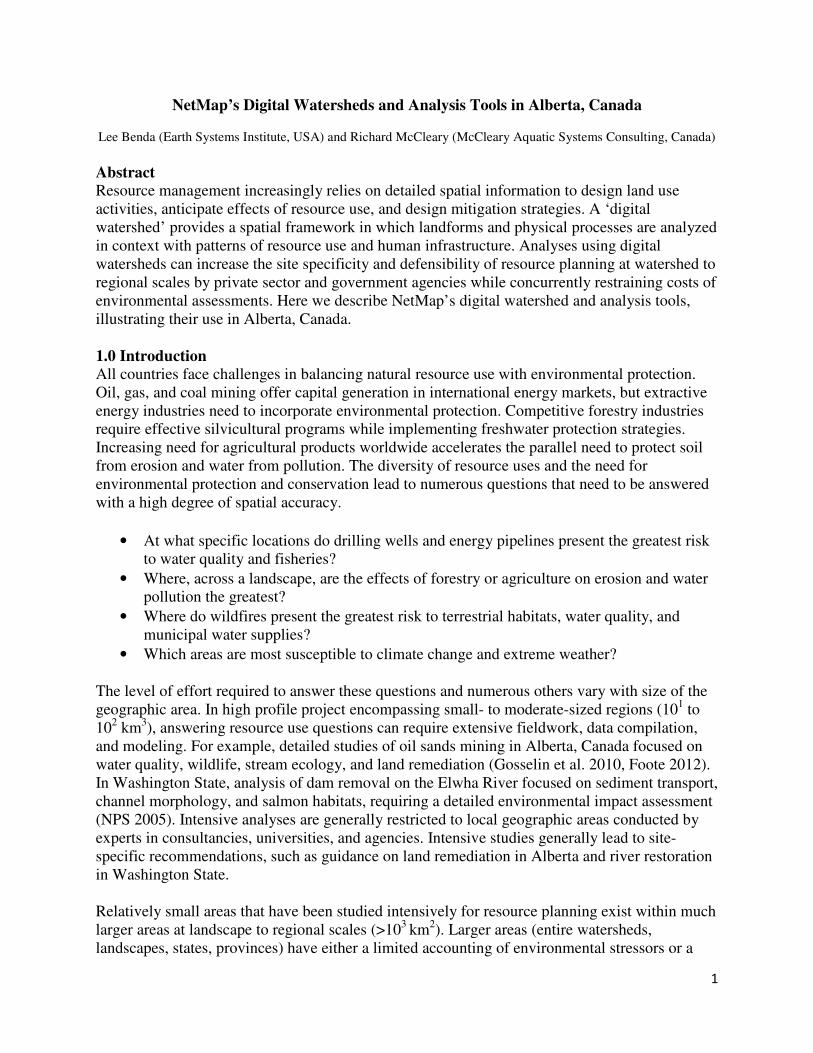
Figure 1. NetMap consists of a digital watershed inclusive of an analytic river network (e.g.,

stream layer) that is coupled to a suite of analysis tools. Desktop watersheds provide a spatial

framework in which landforms and ecological processes are analyzed in context with resource

use activities and infrastructure. NetMap’s analysis tools are designed to work within up to date,

ArcGIS software (ArcMap 10.0 and 10.1). Analysis modules include: 1) Basic Tools, 2) Fluvial

Morphology, 3) Aquatic Habitats, 4) Erosion, 5) Transportation/Energy, and 6) Riparian

Management.

DEMs of varying resolutions can be derived directly from topographic maps. For example,

Alberta maintains a digital (cartographic) stream layer derived from 1: 20,000-scale topography,

that includes a single-line network (AENV 2000). In the last decade, LiDAR (Light Detection

and Ranging) technology has been used to map land surfaces to create high resolution (sub 5 m)

DEMs. The province of Alberta has significant LiDAR coverage that has set the stage for

effective use of digital watersheds in resource use management. For this study, we set NetMap to

employ 1m LiDAR in both the Hinton Wood Products Forest Management Agreement (FMA)

and in the Oldman River basin.

DEMs are used to create shaded relief images, based on elevation, that provide realistic and

attractive depictions of topography in two and three dimension (Figure 1). Shaded relief and

elevation maps are often used qualitatively in resource planning by providing spatial referencing

of landforms such as steep hillsides, river channels, and valley floors to locations of various land

use activities. Cartographic depictions of streams and rivers are digitized from topographic maps,

yielding an important spatial catalogue of stream and river locations. However, they have limited

utility in the context of environmental assessments and resource planning because they lack the

data structure of the digital watershed described below (Figure 2), and they lack attributes

necessary to address resource use questions (Figure 1).

4

2.2 Delineating River Networks and Other Landforms

A river network, inferred from a DEM, is the fundamental landform of a digital watershed; it is

referred to as an “analytic river” (Figure 2) to distinguish it from stream layers that are

cartographic in origin (i.e., not derived directly from a DEM) and to denote its use in analytical

applications involving resource use and risk mitigation.

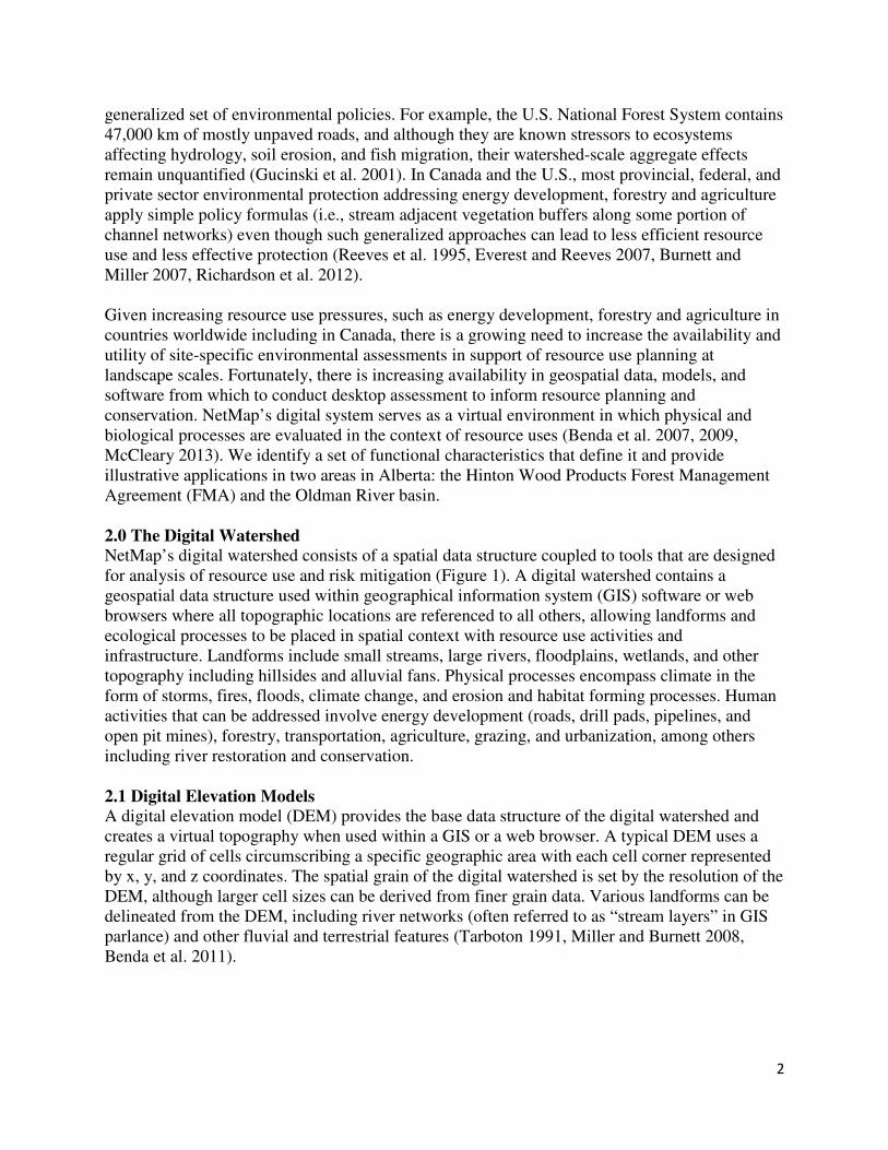
Figure 2. A digital watershed is comprised of a series of elements including (A) DEMs, (B) basin

and subbasin boundaries and lakes, (C) a flow direction grid, (D) an analytic river with segments

set by the spatial grain of the DEM, landforms, discretized roads and pipelines (broken into

segments), (E) connections including downstream-upstream and downslope-upslope transfer of

information, and (F) parameter attribution of stream segments (Table 1). Additional geospatial

information can be integrated into the digital landscape to support various types of

environmental assessments (G). The digital landscape is coupled to a suite of analysis tools

(Figure 1).

The analytic river is derived from surface flow paths inferred from a DEM (Figure 2). Various

algorithms are available to predict flow direction in grid cells and to create a “flow direction

grid” (Jenson and Domingue 1988, Tarboton 1997). Convergence of flow, under certain

constraints, leads to channels; non-convergent flows represent the terrestrial watershed.

5

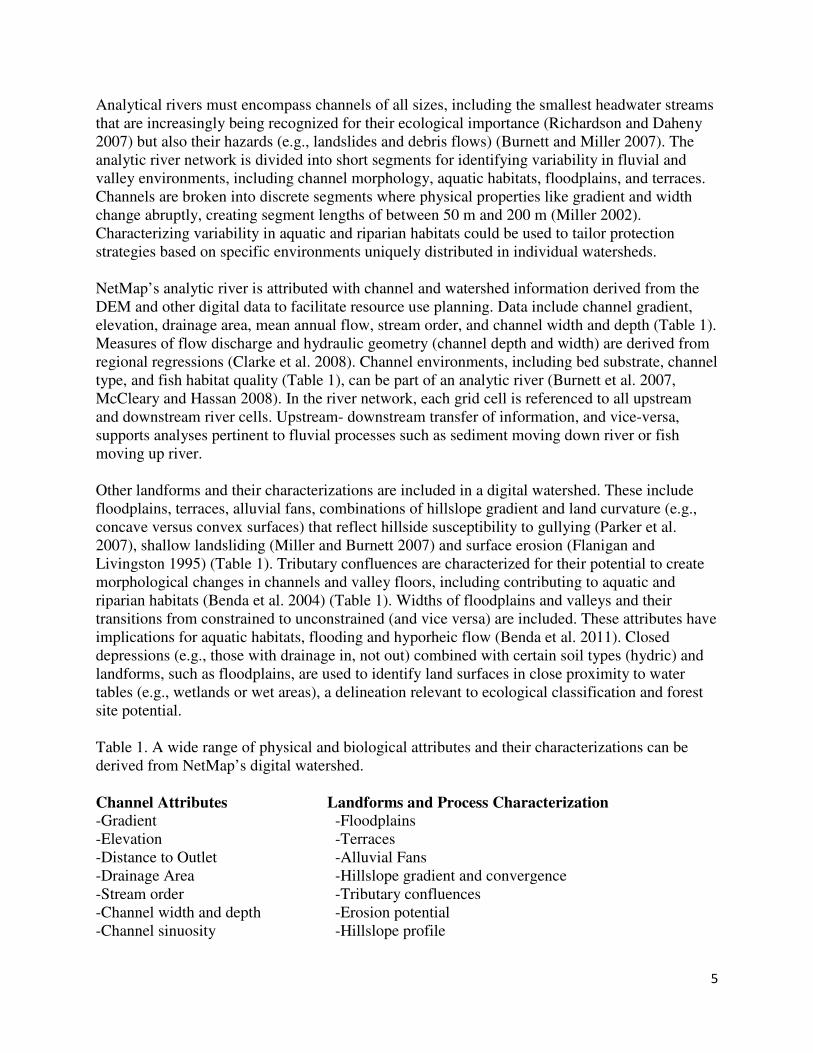
Analytical rivers must encompass channels of all sizes, including the smallest headwater streams

that are increasingly being recognized for their ecological importance (Richardson and Daheny

2007) but also their hazards (e.g., landslides and debris flows) (Burnett and Miller 2007). The

analytic river network is divided into short segments for identifying variability in fluvial and

valley environments, including channel morphology, aquatic habitats, floodplains, and terraces.

Channels are broken into discrete segments where physical properties like gradient and width

change abruptly, creating segment lengths of between 50 m and 200 m (Miller 2002).

Characterizing variability in aquatic and riparian habitats could be used to tailor protection

strategies based on specific environments uniquely distributed in individual watersheds.

NetMap’s analytic river is attributed with channel and watershed information derived from the

DEM and other digital data to facilitate resource use planning. Data include channel gradient,

elevation, drainage area, mean annual flow, stream order, and channel width and depth (Table 1).

Measures of flow discharge and hydraulic geometry (channel depth and width) are derived from

regional regressions (Clarke et al. 2008). Channel environments, including bed substrate, channel

type, and fish habitat quality (Table 1), can be part of an analytic river (Burnett et al. 2007,

McCleary and Hassan 2008). In the river network, each grid cell is referenced to all upstream

and downstream river cells. Upstream- downstream transfer of information, and vice-versa,

supports analyses pertinent to fluvial processes such as sediment moving down river or fish

moving up river.

Other landforms and their characterizations are included in a digital watershed. These include

floodplains, terraces, alluvial fans, combinations of hillslope gradient and land curvature (e.g.,

concave versus convex surfaces) that reflect hillside susceptibility to gullying (Parker et al.

2007), shallow landsliding (Miller and Burnett 2007) and surface erosion (Flanigan and

Livingston 1995) (Table 1). Tributary confluences are characterized for their potential to create

morphological changes in channels and valley floors, including contributing to aquatic and

riparian habitats (Benda et al. 2004) (Table 1). Widths of floodplains and valleys and their

transitions from constrained to unconstrained (and vice versa) are included. These attributes have

implications for aquatic habitats, flooding and hyporheic flow (Benda et al. 2011). Closed

depressions (e.g., those with drainage in, not out) combined with certain soil types (hydric) and

landforms, such as floodplains, are used to identify land surfaces in close proximity to water

tables (e.g., wetlands or wet areas), a delineation relevant to ecological classification and forest

site potential.

Table 1. A wide range of physical and biological attributes and their characterizations can be

derived from NetMap’s digital watershed.

Channel Attributes Landforms and Process Characterization -Gradient -Floodplains

-Elevation -Terraces

-Distance to Outlet -Alluvial Fans

-Drainage Area -Hillslope gradient and convergence

-Stream order -Tributary confluences

-Channel width and depth -Erosion potential

-Channel sinuosity -Hillslope profile

6

-Channel classification -Debris flows

-Fish habitats -Earthflows

2.3 River Network – Terrestrial Coupling Terrestrial landforms are connected to river networks within a digital watershed by grid cell

referencing. Downslope–upslope transfer of information, and vice-versa, addresses processes

such as sediment moving from hillsides to rivers or animals transferring nutrients from streams

to mid-slope forests. Each river cell is linked to adjacent or nearby floodplain, terrace or valley

cells, allowing riparian environments to be coupled to specific reaches of channel. For instance,

riparian forests drive recruitment rates of in-stream wood and are directly related to formation of

fish habitat (e.g., pools, cover), a relationship that ties spatial locations of valley floors and

channels together.

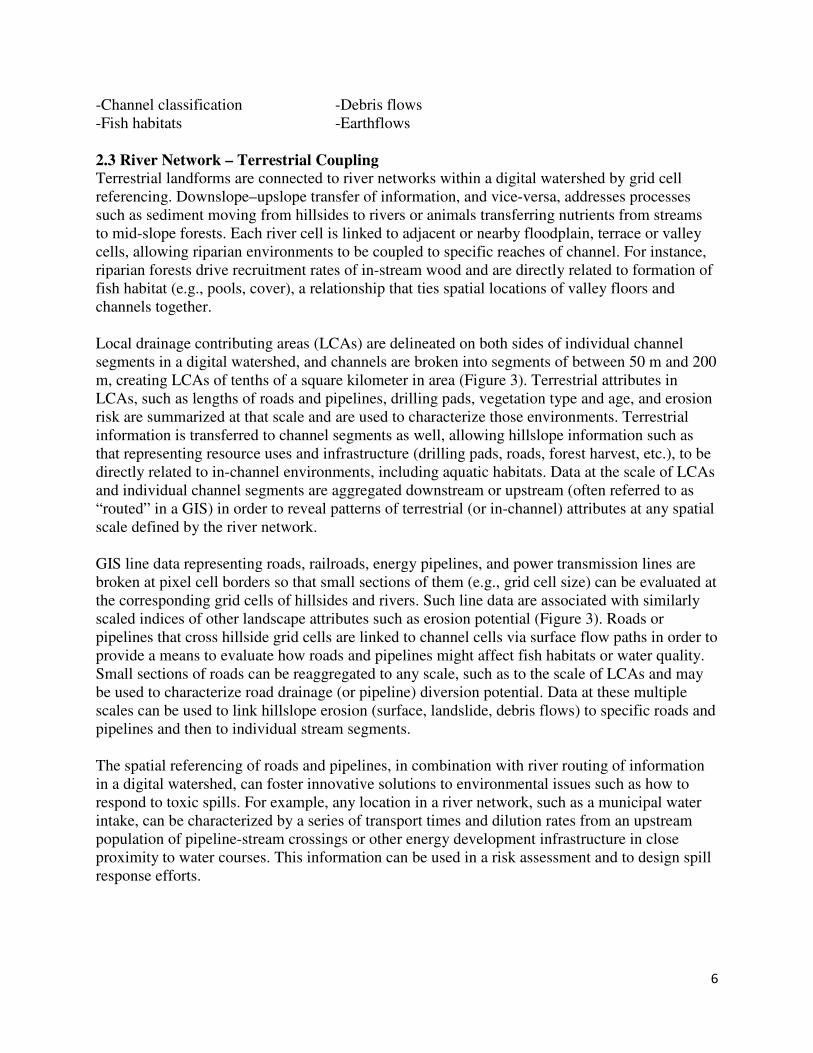
Local drainage contributing areas (LCAs) are delineated on both sides of individual channel

segments in a digital watershed, and channels are broken into segments of between 50 m and 200

m, creating LCAs of tenths of a square kilometer in area (Figure 3). Terrestrial attributes in

LCAs, such as lengths of roads and pipelines, drilling pads, vegetation type and age, and erosion

risk are summarized at that scale and are used to characterize those environments. Terrestrial

information is transferred to channel segments as well, allowing hillslope information such as

that representing resource uses and infrastructure (drilling pads, roads, forest harvest, etc.), to be

directly related to in-channel environments, including aquatic habitats. Data at the scale of LCAs

and individual channel segments are aggregated downstream or upstream (often referred to as

“routed” in a GIS) in order to reveal patterns of terrestrial (or in-channel) attributes at any spatial

scale defined by the river network.

GIS line data representing roads, railroads, energy pipelines, and power transmission lines are

broken at pixel cell borders so that small sections of them (e.g., grid cell size) can be evaluated at

the corresponding grid cells of hillsides and rivers. Such line data are associated with similarly

scaled indices of other landscape attributes such as erosion potential (Figure 3). Roads or

pipelines that cross hillside grid cells are linked to channel cells via surface flow paths in order to

provide a means to evaluate how roads and pipelines might affect fish habitats or water quality.

Small sections of roads can be reaggregated to any scale, such as to the scale of LCAs and may

be used to characterize road drainage (or pipeline) diversion potential. Data at these multiple

scales can be used to link hillslope erosion (surface, landslide, debris flows) to specific roads and

pipelines and then to individual stream segments.

The spatial referencing of roads and pipelines, in combination with river routing of information

in a digital watershed, can foster innovative solutions to environmental issues such as how to

respond to toxic spills. For example, any location in a river network, such as a municipal water

intake, can be characterized by a series of transport times and dilution rates from an upstream

population of pipeline-stream crossings or other energy development infrastructure in close

proximity to water courses. This information can be used in a risk assessment and to design spill

response efforts.

7

Figure 3. The digital watershed includes (A) a routed analytic river with confluences, including

attributes (Table 1). (B) Each segment has a right-left differentiated local contributing area or

LCA (tenths of a square kilometer at a segment length of 100 m). (C) Information contained

within LCAs such as pipeline/road length and erosion potential is transferred to stream segments.

Information is aggregated downstream, revealing patterns of channel and hillslope characteristics

at any spatial scale defined by the channel network (or routed upstream). LCAs support analyses

including identifying overlaps between terrestrial and aquatic environments, including human-

related stressors (such as erosion, wildfire, roads, etc.). (D) Roads (pipelines and power

transmission lines) are broken at pixel borders to link line data to pixel scale information on

factors such as landslide potential. Road pixel segments can also be re-aggregated to predict

factors such as road drainage diversion potential.

NetMap’s data structure allows the cumulative distribution of any watershed or resource use

attribute to be calculated at any scale. This mathematical structure allows terrestrial information

(such as erosion potential) or road and pipeline density (km/km2) to be evaluated in terms of

exceedence frequency or probability. Thus, a planner can quickly assess whether LCAs with the

highest 10% of erosion potential due to roads overlap with the top 10% of the most sensitive

river channels. Identifying such locations could be used to prioritize areas where remedial

efforts, such as road maintenance, would have the greatest benefit to freshwater ecosystems.

The geospatial data structure of a digital watershed is customizable to individual landscapes.

Analytic river networks can be expanded or contracted, and segment lengths and LCAs can be

8

decreased or increased in size, to meet the needs of particular applications. Thus, the data

structure is not fixed, but rather is dynamic, ensuring that analyses remain accurate and relevant.

In addition, knowledge generated within a digital watershed can be transferred to other agency

and private sector stream layers and vice versa.

2.4 High Relief and Low Relief Topography

The flow routing algorithms that create flow direction grids and delineate channel networks

require topography that has measurable energy gradients driven by relief. The greater the relief

and the greater that surface and subsurface flow are driven by topography, the more accurate the

derived surface flow directions and the analytic river network. This straightforward relationship

between topography and flow paths may not exist in areas of low relief and complicated

subsurface geology, such as in the boreal forests of northern Alberta (Devito et al. 2005).

In areas of low relief and where DEMs are insufficient to determine flow gradients in all

locations, optical satellite imagery has been used to map locations of open water in channels and

connected wetlands and sloughs. Particularly in areas of limited forest coverage, satellite

imagery is used to differentiate between land and water based on optical contrast and intensity

where local slope gradient is insufficient to derive the river network (Burnett et al. 2013. Flow

algorithms in NetMap are used to create a digital map of surface water (e.g., water mask) to

create an analytic river. Flow directions are guided by the water mask using monotonically

decreasing channel slopes based on landscape scale elevation gradients. Ray-tracing algorithms

are used to follow a constant velocity wave front confined to the water mask polygons (Burnett

et al. 2013.

Connecting channel-adjacent water bodies to the predicted channel network is yet another

challenge in low relief topography. Mapping connectivity between derived channel networks and

bodies of water such as sloughs, ponds, beaver-dammed channels, and lakes could be done using

algorithms that employ channel-water body proximity as well as other indicators such as

underlying geology or vegetation. The derivation of flow paths and channel networks in low

relief areas will depend on available geospatial data including the resolution of the DEM and

available satellite imagery.

3.0 Digital Watersheds - Tools and Applications

A robust desktop watershed analysis system requires a suite of analysis tools for addressing a

wide range of resource use and conservation questions. NetMap contains approximately 70

analysis tools that work with digital watersheds (and analytic rivers) to address numerous

resource use questions (Benda et al. 2007, 2011; McCleary et al. 2011; Ferandez et al. 2012;

Pickard 2013; Reeves et al. 2013).

• Where are streams and rivers located, including headwaters and what are their attributes?

• Where are floodplains, terraces, and alluvial fans located and which ones present the

most risk to development?

• Where are the top 10% of the best aquatic habitats located in a watershed and where do

they intersect the largest stressors from energy development and forestry?

• Which road segments or pipelines present the greatest 10% of risk to water quality and

aquatic habitats?

9

• What segments of roads or transmission lines are most at risk from slope instability?

• Where does resource development overlap with the top 1% of mass wasting potential?

NetMap’s analysis tools are designed to work within 2013 ArcGIS software, (ArcMap 10.0 and

10.1). Modules include: 1) Basic Tools, 2) Fluvial Morphology, 3) Aquatic Habitats, 4) Erosion,

5) Transportation/Energy, and 6) Riparian Management.

Basic Tools encompass various data query and management functions and includes stream and

hillslope profiling, routing of attributes downstream or upstream, Google Earth interface, risk

analysis, and subbasin classification functions. Fluvial Morphology contains 23 tools and

parameters that provide a wealth of channel physical attributes (see Table 1); network attributes

(stream order, confluence types, drainage density, etc.); several channel and fish habitat

classification methods; floodplain, terrace and alluvial fan mapping; and in-stream wood

accumulation. The Aquatic Habitat module contains 13 tools for predicting fish habitat (resident

and anadromous), beaver habitat, core habitat areas, habitat diversity, and cumulative habitat

length and quality along the channel among others. The Erosion module includes interfaces for

shallow failure, gully formation, debris flow, earthflows, surface erosion, sediment yield, and

sediment delivery.

The Transportation/Energy module contains tools for addressing road or pipeline density at

multiple scales (stream reach, river network, and subbasins), road stability, roads/pipelines in

floodplains, habitat length and quality upstream of all road (or pipeline) crossings, road surface

erosion, and sediment delivery to streams. The Transportation/Energy tools could be used

retrospectively to identify provisional habitat-stressor hotspots across large geographic areas

(energy leases or FMAs) or used prospectively to identify the least at-risk locations for future

roads, pipelines, or energy transmission lines.

The Riparian Management module contains interfaces for radiation loading, in-stream wood

recruitment (stream reach and watershed scale), upslope (mass wasting) wood recruitment, and

vegetation simulation. This tool suite can be used to tailor riparian and stream protection

strategies across diverse landscapes rather than relying on uniform, one-size-fits-all prescriptions

(Pickard 2013, Reeves 2013).

All models contained within the modular ArcMap add-ins are based on the published literature

(for additional information, refer to www.netmaptools.org). All tools are supported by 600 pages

of online hyperlinked technical help materials that cover tool use, scientific background, example

applications, and related reference materials. A critical and necessary element in NetMap is that

all tools work seamlessly with one another to support multi- and interdisciplinary analyses within

the uniform data structure of the digital watershed.

4.0 Illustrative Applications in Alberta

4.1 West Fraser Forest Management Agreement (FMA)

Timber harvesting in Alberta must protect water resources. Traditionally this has been done

through the application of uniform width buffers along streams where little to no forest

management is allowed. However, the uniform buffer paradigm is being challenged because it

may be ecologically inappropriate in some watershed and riparian settings (Richardson et al.

2012, Pickard 2103). New riparian strategies could encourage greater diversity in streamside

10

vegetation (age and composition), allow tailoring of protection based on stream ecological

conditions, promote greater wildfire protection, and create opportunities for in-stream and

riparian restoration. An accurate stream layer, inclusive of headwaters, with associated physical

and biological attributes that can be used for channel classification and fish habitat modeling, is

required to accomplish conventional or more innovate riparian management.

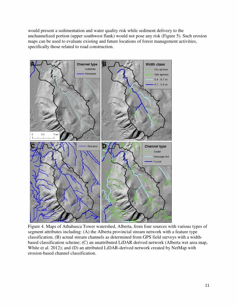
Alberta maintains a digital (cartographic) stream layer (derived from 1: 20,000-scale topography)

that includes a single-line network (AENV 2000). Rivers larger than 20 m in width are well

represented, but smaller watercourses are less accurately depicted. For example, channels less

than 5 m in width are often classed as “indefinite” because they are poorly distinguished

(McCleary and Hassan 2008). Many streams less than 1.5 m wide are obscured beneath

vegetation and are not included in the cartographic stream layer (McCleary 2011) (Figure 4A).

The inadequately represented headwater streams, which comprise more than 60% of the total

length of the river network in the Rocky Mountain Foothills region (McCleary 2011), are

ecologically important and require regulatory protection (ASRD 2008). Alberta also has a

stream layer (derived from 1 m DEMs) that accurately identifies the majority of the channel

network (Figure 4C) and includes probable locations of land surfaces that are in close proximity

to water tables (“wet areas”) (White et al. 2012). The wet areas network contains long segment

lengths (kilometers), lacks physical attributes, is not routed, and is not coupled to the DEM (e.g.,

there is an absence of downslope, upslope routing). Therefore, this network is limited in its use

in environmental analyses (e.g., Figures 1 and 2).

Hinton Wood Products (HWP), a Division of West Fraser Mills Ltd., in conjunction with the

Foothills Research Institute and Earth Systems Institute, applied NetMap using 1-meter DEMs to

support channel and fish habitat classification within a digital watershed (10,000 km2)

(McCleary 2011). GPS-based field surveys were used to calibrate and validate NetMap’s

analytic network (Figure 4B). Channel attributes in the analytic river required for classifying

channels and habitats include drainage area, channel gradient, mean basin slope, floodplains and

longitudinal profiles (McCleary 2011). The resulting characterization of channel types (uplands,

swales, seepage-fed channels, fluvial channels, and floodplains) and fish habitats (e.g., bull trout

[Salvelinus confluentus] and rainbow trout [O. mykiss]) allows HWP to incorporate them in

forest management planning, including in designing riparian protection zones (Figure 4D).

NetMap’s floodplain mapping will be used to map riparian zones at a range of elevations above

the channel (to match field observations). This data can be used to consider how floodplain and

low terrace extent and elevation relate to channel environments and proximity to water table.

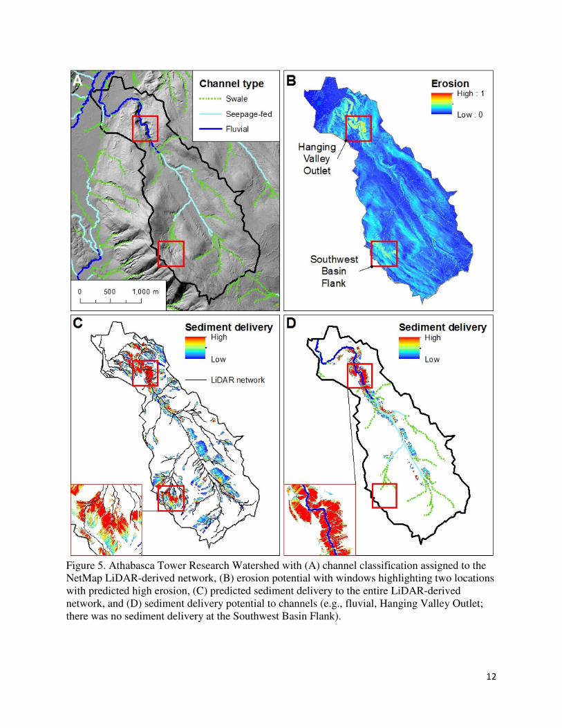
Another need in the Hinton Wood Products FMA is to identify landforms with a high

susceptibility to erosion and sediment delivery to stream channels. One of NetMap’s indices of

erosion susceptibility is based on slope steepness and planform curvature (Miller and Burnett

2007), attributes well recognized in controlling the potential for shallow landsliding and gullying

(Dietrich and Dunne 1978, Sidle 1987). The analysis revealed great spatial variability in hillside

erosion susceptibility across the FMA. For example, within the Athabasca Tower Research

Watershed, erosion potential is high at only two locations–along the inner gorge of the outlet

stream draining a hanging valley and at the southwest flank of the basin (Figure 5). The

predicted erosion potential, when combined with channel classification, is used to evaluate risk

to aquatic biota and water quality. For instance, sediment delivery to the fluvial channel network

11

would present a sedimentation and water quality risk while sediment delivery to the

unchannelized portion (upper southwest flank) would not pose any risk (Figure 5). Such erosion

maps can be used to evaluate existing and future locations of forest management activities,

specifically those related to road construction.

Figure 4. Maps of Athabasca Tower watershed, Alberta, from four sources with various types of

segment attributes including: (A) the Alberta provincial stream network with a feature type

classification, (B) actual stream channels as determined from GPS field surveys with a width-

based classification scheme; (C) an unattributed LiDAR derived network (Alberta wet area map,

White et al. 2012); and (D) an attributed LiDAR-derived network created by NetMap with

erosion-based channel classification.

12

Figure 5. Athabasca Tower Research Watershed with (A) channel classification assigned to the

NetMap LiDAR-derived network, (B) erosion potential with windows highlighting two locations

with predicted high erosion, (C) predicted sediment delivery to the entire LiDAR-derived

network, and (D) sediment delivery potential to channels (e.g., fluvial, Hanging Valley Outlet;

there was no sediment delivery at the Southwest Basin Flank).

13

4.2 Oldman River Basin

The Alberta Provincial Government, in conjunction with Earth Systems Institute and the

Foothills Research Institute, evaluated the use of digital watersheds (NetMap) for assessing

cumulative watershed effects (CWE) in the Oldman River basin (McCleary 2013). An analysis

of CWE contains three steps: 1) characterize relevant watershed landforms and processes, 2)

estimate how land use and infrastructures affect them, and 3) determine whether altered

landscape processes impact important resources and whether mitigation is warranted (WDNR

2011).

There are a several potential stressors in the Oldman watershed (3,000 km2) including grazing,

forestry, residential development, and energy pipelines. NetMap’s analysis was used to: 1) create

a digital watershed, including an accurate and attributed analytic stream network, 2) predict fish

habitat, 3) map floodplains and terraces at various elevations above the channel, and 4) predict

road (and ATV trail) drainage connectivity, surface erosion, and sediment delivery to streams

(McCleary 2013). Although NetMap contains numerous other attributes and tools, these four

were chosen for the demonstration analysis.

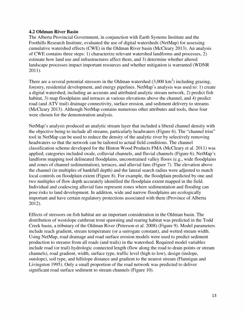
NetMap’s analysis produced an analytic stream layer that included a liberal channel density with

the objective being to include all streams, particularly headwaters (Figure 6). The “channel trim”

tool in NetMap can be used to reduce the density of the analytic river by selectively removing

headwaters so that the network can be tailored to actual field conditions. The channel

classification scheme developed for the Hinton Wood Products FMA (McCleary et al. 2011) was

applied; categories included swale, colluvial channels, and fluvial channels (Figure 6). NetMap’s

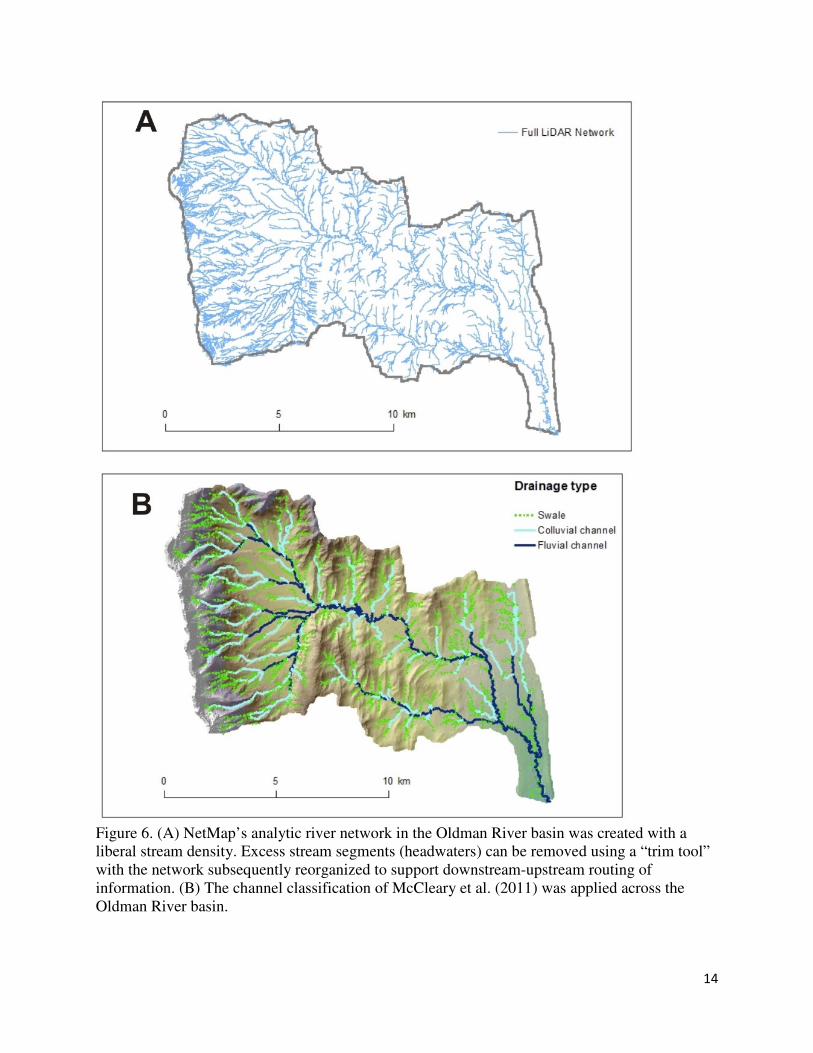
landform mapping tool delineated floodplains, unconstrained valley floors (e.g., wide floodplains

and zones of channel sedimentation), terraces, and alluvial fans (Figure 7). The elevation above

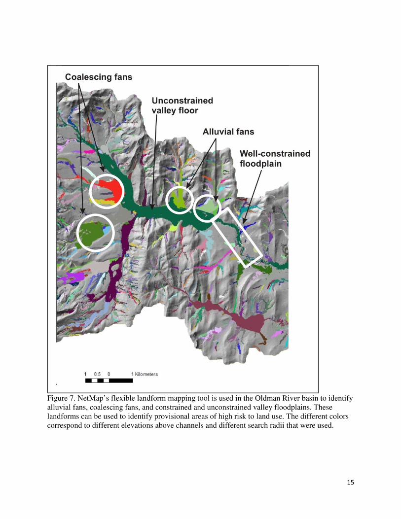
the channel (in multiples of bankfull depth) and the lateral search radius were adjusted to match

local controls on floodplain extent (Figure 8). For example, the floodplain predicted by one and

two multiples of flow depth accurately identified the floodplain extent mapped in the field.

Individual and coalescing alluvial fans represent zones where sedimentation and flooding can

pose risks to land development. In addition, wide and narrow floodplains are ecologically

important and have certain regulatory protections associated with them (Province of Alberta

2012).

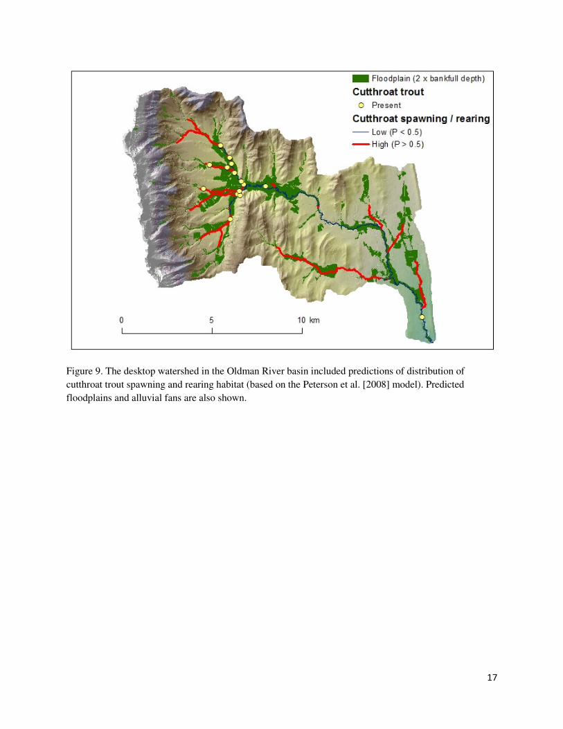
Effects of stressors on fish habitat are an important consideration in the Oldman basin. The

distribution of westslope cutthroat trout spawning and rearing habitat was predicted in the Todd

Creek basin, a tributary of the Oldman River (Peterson et al. 2008) (Figure 9). Model parameters

include reach gradient, stream temperature (or a surrogate constant), and wetted stream width.

Using NetMap, road drainage and road surface erosion models were used to predict sediment

production to streams from all roads (and trails) in the watershed. Required model variables

include road (or trail) hydrologic connected length (flow along the road to drain points or stream

channels), road gradient, width, surface type, traffic level (high to low), design (inslope,

outslope), soil type, and hillslope distance and gradient to the nearest stream (Flannigan and

Livingston 1995). Only a small proportion of the road network was predicted to deliver

significant road surface sediment to stream channels (Figure 10).

14

Figure 6. (A) NetMap’s analytic river network in the Oldman River basin was created with a

liberal stream density. Excess stream segments (headwaters) can be removed using a “trim tool”

with the network subsequently reorganized to support downstream-upstream routing of

information. (B) The channel classification of McCleary et al. (2011) was applied across the

Oldman River basin.

15

Figure 7. NetMap’s flexible landform mapping tool is used in the Oldman River basin to identify

alluvial fans, coalescing fans, and constrained and unconstrained valley floodplains. These

landforms can be used to identify provisional areas of high risk to land use. The different colors

correspond to different elevations above channels and different search radii that were used.

16

Figure 8. Terrain features (A and B) including the field delineated 50-year floodplain for two Todd Creek

reaches linked to NetMap’s LiDAR-derived analytic river. The area indicated as floodplain was inundated

during flood stage equivalent to two bankfull depths. The terrain features are linked to UNB’s wet areas

map (C and D). Using NetMap’s flexible landform mapping tool, the terrain features are linked to

predicted floodplains (E and F).

17

Figure 9. The desktop watershed in the Oldman River basin included predictions of distribution of

cutthroat trout spawning and rearing habitat (based on the Peterson et al. [2008] model). Predicted

floodplains and alluvial fans are also shown.

18

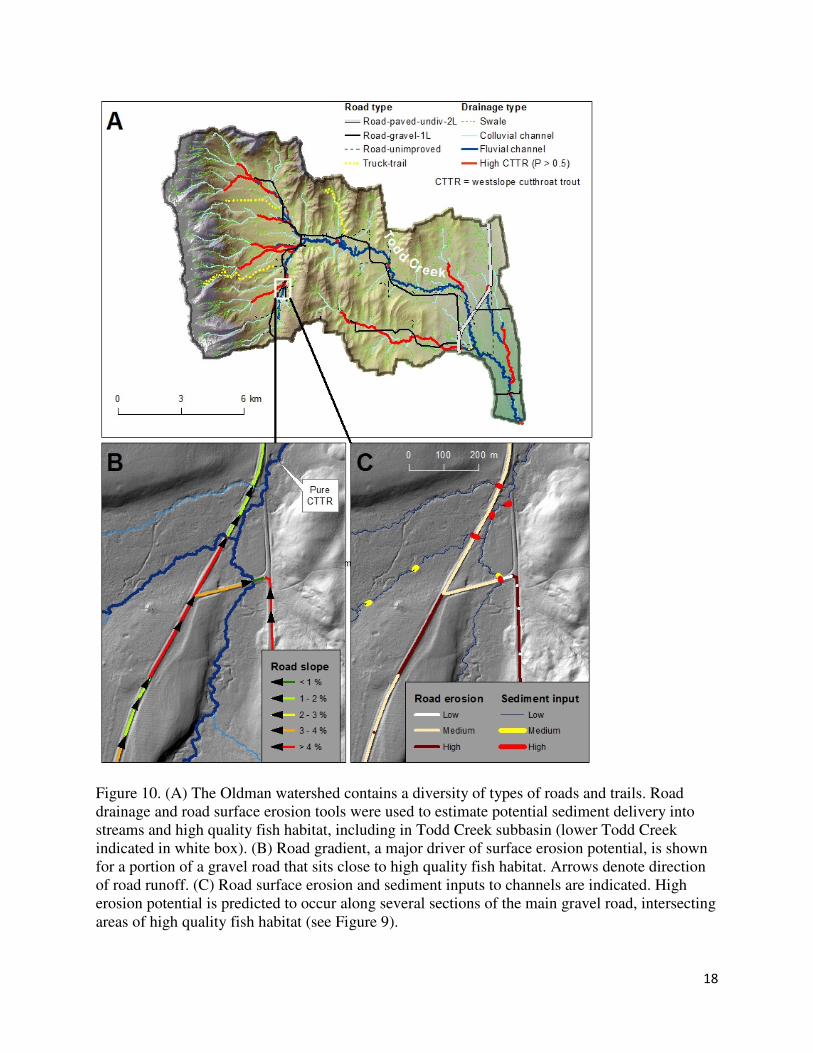
Figure 10. (A) The Oldman watershed contains a diversity of types of roads and trails. Road

drainage and road surface erosion tools were used to estimate potential sediment delivery into

streams and high quality fish habitat, including in Todd Creek subbasin (lower Todd Creek

indicated in white box). (B) Road gradient, a major driver of surface erosion potential, is shown

for a portion of a gravel road that sits close to high quality fish habitat. Arrows denote direction

of road runoff. (C) Road surface erosion and sediment inputs to channels are indicated. High

erosion potential is predicted to occur along several sections of the main gravel road, intersecting

areas of high quality fish habitat (see Figure 9).

19

The main one-lane gravel road is of special concern due to its multiple crossings over high value

westslope cutthroat trout habitat, relatively high traffic levels, and regular road maintenance. The

road follows the mainstream of Todd Creek and presents a potential risk to high value fisheries

(Figure 10). Forest roads can drain directly into streams and they may have other drain points

into forested hillslopes. NetMap calculates the length of hydrologically connected road segments

using topography (DEM). Small road segment lengths allowed close examination of road

gradients, their proximity to streams, and predicted road surface erosion. Predicted road erosion

was ranked low, medium, or high for individual segments, including referencing sediment

delivery to streams (Figure 10D). Only a few road segments of the busiest gravel road presented

a sedimentation risk to high value habitat. Once validated, the predictions could be used to

design and implement sediment reduction activities at specific locations (i.e., those areas that

would yield the greatest benefit to fisheries).

5.0 Conclusions

Building digital watersheds at the scale of landscapes, regions, and provinces has the potential to

advance how resource use is planned and implemented in the context of physical and biological

attributes of landscapes, including in Alberta, Canada. It can significantly reduce stressor-habitat

interactions and promote more sustainable land use in Alberta and beyond, making resource use

more defensible, while restraining costs of environmental assessments. Building a digital

watershed using a consistent data structure within a GIS or in online browsers has the potential to

serve as a communication medium to connect science and technology developers with the large

number of information consumers.

NetMap’s use of digital watersheds and tools as illustrated in the Hinton Wood Products FMA

and the Oldman watersheds can range in level of effort. An initial analysis includes streams and

rivers (the analytic river) with numerous attributes (Table 1), channel response types, aquatic

(fish) habitat quality and distribution, erosion source areas, sediment delivery, environmental

stressors related to roads and pipelines, and riparian environments. This level of information will

allow experts and generalists (e.g., resource managers and planners) alike to predict locations

where land use stressors intersect sensitive habitats with a high degree of specificity. For

example, a planner will be able to identify provisional hotspots where the top 5% of the highest

road surface erosion overlaps the top 5% of fish habitat quality or where the highest 10% of

hillslope erosion potential is located in a watershed. Field validation of predicted attributes

should be a component of desktop analyses; the inclusion of field data and other field

measurements is recommended to make desktop analysis more robust.

A more detailed analysis could involve 1) creating spill response maps using the routing

capabilities in NetMap, 2) coupling wildfire risk to erosion potential (surface and mass wasting),

3) supporting a watershed scale sediment budget or 4) assessing riparian management in the

context of in-stream wood recruitment and thermal loading. Assessing the role of vegetation

removal on slope stability (landslides and debris flows) could be included, as well as the role of

climate change on altering flow regimes and impacting fish habitat. This level of analysis might

also require that detailed field surveys be performed in which models are calibrated with local

data.

20

Acknowledgements

NetMap’s digital watershed with analysis tools is the result of partnerships with the U.S. Forest

Service, U.S. Bureau of Land Management, NOAA-Fisheries, the U.S. EPA, and NGOs since

2008. We greatly appreciate funding from Alberta Environment and Sustainable Resource

Development and Hinton Wood Products, a division of West Fraser Mills Ltd., to conduct the

desktop watershed analyses. Additional information on NetMap can be seen at:

www.netmaptools.org.

References Alberta Environment (AENV). 2000. Base features data specifications, Rev. 2.0. DRAFT under review.

Resource Data Division, Land and Forest Service, Alberta Environment. http://lists.refractions.net/msrm-

cwb/docs/Alberta/BaseFeatures%20Spec_V%202.pdf (Accessed Dec. 30, 2012).

Alberta Sustainable Resource Development (ASRD). 2008. Alberta timber harvest planning and operating

ground rules framework for renewal. Alberta Sustainable Resource Development, Public Lands and

Forests Division, Forest Management Branch. 0-86499-919-4.

http://www.srd.alberta.ca/LandsForests/ForestManagement/ForestManagementPlanning/documents/Anne

x_4_draft_Jan_15_08Final.pdf [accessed 4 January 2013].

Benda L, Poff NL, Miller D, Dunne T, Reeves GH, Pess GH, Polluck M. 2004. The network dynamics

hypothesis: How channel networks structure riverine habitats. Bioscience 54: 413–427.

Benda, L., D. J. Miller, K. Andras, P. Bigelow, G. Reeves, and D. Michael. 2007. NetMap: A new tool in

support of watershed science and resource management. Forest Science 52:206-219.

Benda, L., D. Miller, S. Lanigan, and G. Reeves. 2009. Future of applied watershed science at regional

scales. EOS, Transaction American Geophysical Union 90:156-157.

Benda, L., Miller, D., and Barquín, J. 2011. Creating a catchment scale perspective for river restoration,

Hydrol. Earth Syst. Sci., 15, 2995-3015, doi:10.5194/hess-15-2995-2011.

Benda, L. 2012. Analysis of roads in support of restoration planning in the Clearwater River, western

Montana using NetMap. http://www.netmaptools.org/Pages/Clearwater_NetMap_final.pdf

Burnett, K., and D. Miller, 2007. Streamside Policies for Headwater Channels: An Example Considering

Debris Flows in the Oregon Coastal Province. Forest Science 53(2):239-253.

Burnett, K. M., et al. 2007. Distribution of salmon-habitat potential relative to landscape characteristics

and implications for conservation. Ecological Applications 17(1): 66-80.

Burnett, K. M., D. J. M., Rick Guritz, Mark A. Meleason, Ken Vance-Borland, Rebecca Flitcroft,

Matthew J. Nemeth, Justin Priest, Nicholas A. Som, Christian E. Zimmerman. 2013. 2011 Arctic-Yukon-

Kuskowkwin Sustainable Salmon Initiative. Project Final Report: 79.

Clarke, S.E., Burnett, K.M., and Miller, D.J. 2008. Modeling streams and hydrogeomorphic attributes in

Oregon from digital and field data. Journal of the American Water Resources Association 44(2): 459-477.

Collins, B. D. and G. R. Pess. 1997. Critique of Washington's Watershed Analysis Programs (Bigelow).

Journal of American Water Resources Association 33(5): 997-1010.

21

Creed, I.F., Sass, G.Z., Wolniewicz, M.B., and Devito, K.J. 2008. Incorporating hydrologic dynamics into

buffer strip design on the sub-humid Boreal Plain of Alberta. Forest Ecology and Management 256(11):

1984-1994.

Dietrich, W. E. and T. Dunne. 1978. Sediment budget for a small catchment mountainous terrain.

Zietshrift fur Geomorphologie: 191-206.

Devito, K., Creed, I., Gan, T., Mendoza, C., Petrone, R., Silins, U., and Smerdon, B. 2005. A framework

for broad-scale classification of hydrologic response units on the Boreal Plain: is topography the last thing

to consider? Hydrological Processes 19(8): 1705-1714. <Go to ISI>://000229232800010.

Environmental Protection Agency (USEPA). 2003. Watershed analysis and management guide to states

and communities. http://water.epa.gov/learn/training/wacademy/wam2003_index.cfm

Everest, F. H., and G. H. Reeves. 2007. Riparian and aquatic habitats of the Pacific Northwest and

Southeast Alaska: Ecology, Management History and Potential Management Strategies. Gen.Tech. Rep.

PNW-GTR-692 Pacific Northwest Research Station.

Fernandez, D., J. Barquin, M. Alvarez-Cabria, and F.J. Penas. 2012. Quantifying the performance of

automated GIS-based geomorphological approaches for riparian zone delineation using digital elevation

models. Hydrol. Earth Syst. Sci., 16, 3851–3862, www.hydrol-earth-syst-sci.net/16/3851/2012/.

Flanagan, D. C., and S. J. Livingston. 1995. WEPP User Summary: USDA–Water Erosion Prediction

Project (WEPP). NSERL Report No. 11. W. Lafayette, Ind.: USDA–ARS National Soil Erosion Research

Laboratory.

Foote, L. 2012. Threshold considerations and wetland reclamation in Alberta’s Mineable Oil Sands.

Ecology and Society V. 17, No. 1: 35pp

Gosselin, P., S. Hrudey, A. Naeth, A Plourde, R. Therrien, G. Van Der Kraak, and Z. Xu. 2010.

Environmental and health impacts of Canada’s Oils Sands Industry. The Royal Society of Canada (Expert

Panel). 22pp.

Gucinski, H. H., H. B., M. J. Furniss, R. R. Ziemer . 2001. Forest roads: a synthesis of scientific

information. U.S. Department of Agriculture, Forest Service, General Technical Report PNW-GRT-509,

Portland Oregon: 103.

Gregory, S. V., et al., Eds. 2003. The Ecology and Management of Wood in World Rivers. Bethesda,

Maryland, American Fisheries Society.

Hassan, M. A., M. Church, T.E. Lisle, F. Brardinoni, L. Benda, G.E. Grant. 2005. Sediment transport and

channel morphology in small forested streams. Journal of the American Water Resources Association

41(4): 853-876.

Jenson SK and Domingue JO, 1988. Software tools to extract topographic structure from digital

elevation data for geographic inform

McCleary, R.J., and Hassan, M.A. 2008. Predictive modeling and spatial mapping of fish distributions in

small streams of the Canadian Rocky Mountain foothills. Canadian Journal of Fisheries and Aquatic

Sciences 65: 319-333.

22

McCleary, R.J. 2011. Landscape organization based on application of the process domain concept for a

glaciated foothills region. PhD thesis. University of British Columbia. Vancouver, B.C.

https://circle.ubc.ca/bitstream/handle/2429/32154/ubc_2011_spring_mccleary_richard.pdf?sequence=1

(Accessed June 14, 2012).

McCleary, R. J., M.A. Hassan, D. Miller and R.D. Moore. 2011 Spatial organization of process domains

in headwater drainage basins of a glaciated foothills region with complex longitudinal profiles. Water

Resources Research, Vol. 47. Pp17.

McCleary, R.J. 2013. A cumulative watershed effects assessment template for the Eastern Slopes: the

geomorphic and riparian components with a case study of Todd Creek. Report completed for the Foothills

Research Institute.

Miller, D. 2002. Program for DEM analysis, in Landscape Dynamics and Forest Management. Gen. Tech.

Rep. RMRS-GTR-101CD, U.S.D.A. Forest Service, Rocky Mountain Research Station, Fort Collins, CD-

ROM.

Miller, D. J., and K. M. Burnett, 2007. Effects of forest cover, topography, and sampling extent on the

measured density of shallow, translational landslides, Water Resources. Res., 43, W03433,

doi:10.1029/2005WR004807.

Miller, D.J., and K. M. Burnett, 2008. A probabilistic model of debris-flow delivery to stream channels

demonstrated for the Coast Range of Oregon, USA. Geomorphology 94:184-205,

doi:10.1016/j.geomorph.2007.05.009

Montgomery, D. R., et al. 1995. Watershed Analysis as a Framework for Implementing Ecosystem

Management. Water Resources Bulletin 31(3): 369-386.

Naiman, R. J. and R. E. Bilby. 1998. River Ecology and Management in the Pacific Coastal Ecoregion.

River Ecology and Management: Lessons From the Pacific Coastal Ecoregion. New York, Springer-

Verlag. Chapter 1: 1-9.

National Park Service (NPS). 2005. Elwha River ecosystem restoration implementation. Final

Environmental Impact Statement. National Park Service. 336pp.

Oregon Watershed Enhancement Board (OWEB). 1999. Oregon Watershed Assessment Manual.

http://www.oregon.gov/OWEB/pages/docs/pubs/or_wsassess_manuals.aspx

Parker, C., C. Thorne, R. Bingner, R. Wells, D. Wilcox. (2007. Automated Mapping of Potential for

Ephemeral Gully Formation in Agricultural Watersheds. National Sedimentation Laboratory, Publication

No. 56.

Peterson, D. P. B. E. R., J. B. Dunham, K. D. Fausch, M. K. Young, Michael. 2008. Analysis of trade-offs

between threats of invasion by nonnative brook trout (Salvelinus fontinalis) and intentional isolation for

native westslope cutthroat trout (Oncorhynchus clarkii lewisi). Canadian Journal of Fisheries and Aquatic

Science 65: 557-573.

Pickard, B.R. 2013. Keying forest stream protection to aquatic ecosystem values in multi-ownership

watersheds. MSc. Thesis, Oregon State University, Corvallis, OR. 150 p.

23

Province of Alberta. 2012. Water Act.

http://www.qp.alberta.ca/1266.cfm?page=w03.cfm&leg_type=Acts&isbncln=9780779733651 (Accessed

April 18, 2013).

Reeves, G.H., L.E. Benda, K.M. Burnett, P.A. Bisson, and J.R. Sedell. 1995. A disturbance-based

ecosystem approach to maintaining and restoring freshwater habitats of evolutionarily significant units of

anadromous salmonids in the Pacific Northwest. American Fisheries Society Symposium 17: 334-349.

Reeves, G.H., B.R. Pickard, and K.N. Johnson. 2013. Alternative Riparian Buffer Strategies for Matrix

Lands of BLM Western Oregon Forests That Maintain Aquatic Ecosystem Values.

Reid, L. M. and T. Dunne. 1996. Rapid Construction of Sediment Budgets for Drainage Basins.

Cremlingen, Germany, Catena-Verlag.

Reid, L. 1998. Cumulative watershed effects and watershed analysis. Pacific Coastal Ecoregion. R.

Naiman and R. Bilby: 476-501.

Rich, C., T. McMahon, B. Rieman, and W. Thompson. 2003. Influence of local habitat, watershed, and

biotic features on bull trout occurrence in Montana streams. Transactions of the American Fisheries

Society 132:1053–1064.

Richardson, J. and R. Danehy. 2007. A Synthesis of the Ecology of Headwater Streams and their Riparian

Zones in Temperate Forests. Forest Science 53(2):131–147.

Richardson, J. S., R. J. Naiman, P. A. Bisson. 2012. How did fixed-width buffers become standard

practice for protecting freshwaters and their riparian areas from forest harvest practices. Freshwater

Science 31(1): 232-238.

Sidle, R. C. 1987. A dynamic model of slope stability in zero-order basins. IAHS Publ. 165: 101-110.

Tarboton, D. G., R.L. Bras, and I. Rodriguez-Iturbe. 1991. On the extraction of channel networks from

digital elevation data. Hydrological Processes 5: 81-100.

Tarboton, D.G. 1997. A new method for the determination of flow directions and upslope areas in grid

digital elevation models, Water Resources Research, 33 (2), 309-319.

US Geological Survey. 2012. National Hydrography Dataset. http://nhd.usgs.gov/.

US Environmental Protection Agency (EPA). 2003. Watershed Analysis and Management (WAM) Guide

for States and Communities. EPA publication 841B03007 .

http://water.epa.gov/learn/training/wacademy/upload/2005_02_18_watershed_wacademy_wam2003_wa

mguide-text.pdf

Washington Department of Natural Resources (WDNR). 1992, 2011. Forest Practices Board Manual,

Section 11: Methodology for conducting watershed analysis.

http://www.dnr.wa.gov/publications/fp_wsa_manual_part_1_8.pdf (Accessed Feb. 18, 2013).

White, B., J. Ogilvie, D. Campbell, D. Hiltz, B. Gauthier, H. Chisholm, J. Wen, P. Murphy, and P. Arp.

2012. Using the cartographic depth-to-water index to locate small streams and associated wet areas across

landscapes. Canadian Water Resources Journal 37(4): 333-347.