Lectures Remote Sensing

GEOMETRICAL ASPECTSAND MAPPING OF RS

dr.ir. Jan Clevers

Centre of Geo -InformationEnvironmental Sciences

Wageningen UR

Geometrical Aspects and Mapping of RS

• Importance of geometry• Image matching• Resampling

(L&K section 7.2)

• Sensor geometry(L&K sections 5.6 and 5.7)

Wageningen UR 2010

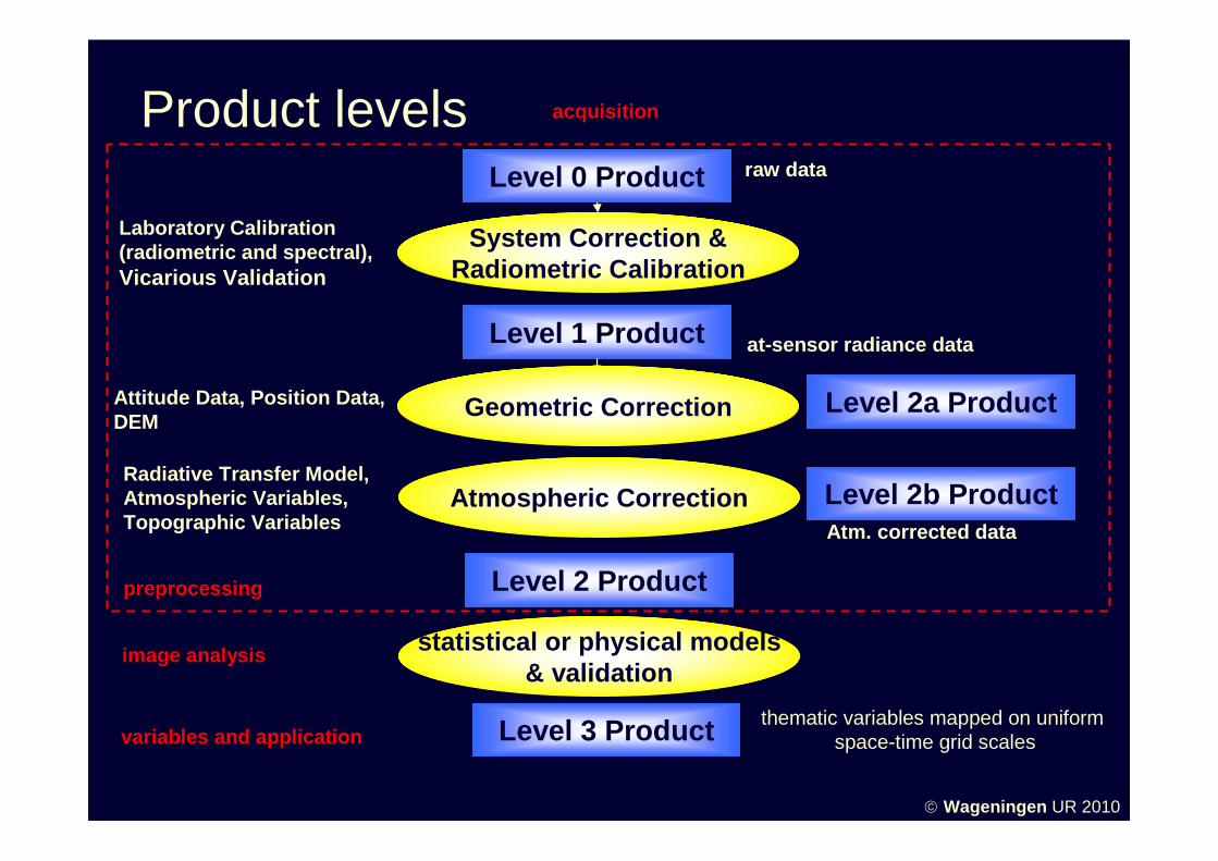
Product levels

Level 1 Product

System Correction &Radiometric Calibration

Level 0 Product

Level 2 Product

Laboratory Calibration(radiometric and spectral), Vicarious Validation

Attitude Data, Position Data, DEM

Radiative Transfer Model,Atmospheric Variables,Topographic Variables

Level 2a Product

raw data

at-sensor radiance data

Level 2b ProductAtm. corrected data

Geometric Correction

Atmospheric Correction

statistical or physical models& validation

Level 3 Product thematic variables mapped on uniform space-time grid scales

preprocessing

image analysis

acquisition

variables and application

Wageningen UR 2010

Why Is Geometry Important?

Mutual comparison of images• multi-spectral• multi-sensor• multi-level• multi-temporal

Comparison with and use of existing data (maps, GIS) for:• interpretation• mapping (geometry, thematics)• building data base (selection, conversion, aggregation, etc)

Wageningen UR 2010

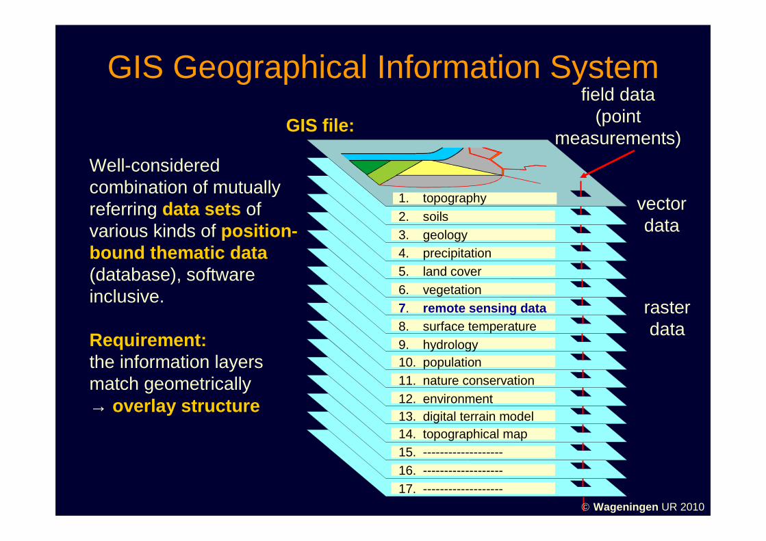
Well-considered combination of mutually referring data sets of various kinds of position-bound thematic data(database), software inclusive.

Requirement:the information layersmatch geometrically→ overlay structure

rasterdata

GIS file:

field data(point

measurements)

vectordata

GIS Geographical Information System

1. topography

2. soils3. geology4. precipitation5. land cover6. vegetation7. remote sensing data8. surface temperature9. hydrology10. population11. nature conservation12. environment13. digital terrain model14. topographical map15. -------------------16. -------------------17. -------------------

Wageningen UR 2010

Image Matching

Image matching(using control points)

Wageningen UR 2010Master or reference Slave or input

image geometry

(i,j)

map geometry

(x,y)

Example airborne Daedalus image

Wageningen UR 2010

Wageningen UR 2010

master

slaveorientated to the master

Image Matching -2-

Wageningen UR 2010

master

slaveorientated to the master

Image Matching -3-

The transformation coefficients are determined using ground control points(GCPs)

GCPs in TIR image

Wageningen UR 2010

GCP selection in Landsat-TM image

Wageningen UR 2010

Image matching TM band 4, 1984 (red) and 1986 (green)

Wageningen UR 2010

Image Matching -4-master

slave

map configuration in digital raster format

or: image raster

image raster

or: map configuration

master

transformed slave

A

B

X

Y

X

Y

x

y

x

y

Wageningen UR 2010

A: Transformation x = ƒ(X,Y) + u

y = g(X,Y) + v

• parametric (flight parameters)

• non-parametric (ground control points)

B: Resampling

Wageningen UR 2010

Steps Image Matching

Trend model: transformation using polynomials(first, second, third order)

x = a1 + a2X + a3Y + a4X2 + a5XY + a6Y2 + … + uy = b1 + b2X + b3Y + b4X2 + b5XY + b6Y2 + … + v

residualsDetermination of the coefficients a1 …. a10, b1 …. b10 usingground control points:1 X1 Y1 X1

2 X1Y1 Y12 X1

3 X12Y1 X1Y1

2 Y13 a1 b1 x1 y1 u1 v1

• = -1 Xn Yn Xn

2 XnYn Yn2 Xn

3 Xn2Yn XnYn

2 Yn3 a10 b10 xn yn un vn

A x B v

in matrix notation: A • x = B - v Wageningen UR 2010

Transformation

Number of GCPs

• first order polynomial → n ≥ 3

• second order polynomial → n ≥ 6• third order polynomial → n ≥ 10

n = number of ground control points

Illustration from curve fitting to reinforce the potentially poor behaviour of high order mathematical functions when used to extrapolate

best third order

best second order

best first order

x

y

Wageningen UR 2010

Correction of geometric distortion

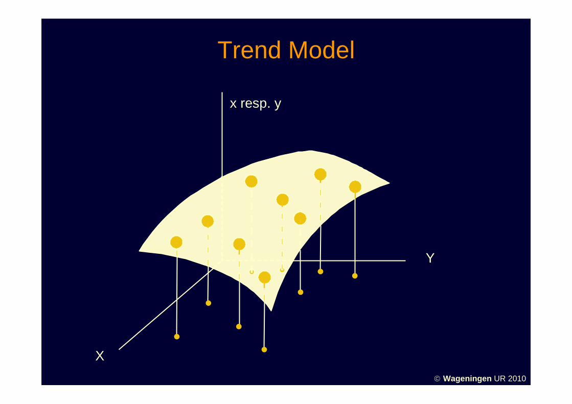
Trend Model

Y

X

x resp. y

Wageningen UR 2010

Facet Model

x resp. y

Y

X

Wageningen UR 2010

After the transformation, a resampling of the pixel values is performed• nearest neighbour• bilinear interpolation• cubic convolution pixel arrangement 1

pixel arrangement 2

pixel arrangement 1 = input (distorted)pixel arrangement 2 = output (corrected)

ab

bb

c c c c

c

c

c c c c

c

c

Wageningen UR 2010

Resampling

Nearest neighbour:the value of the output pixel is taken to be that of the input pixel nearest to which it maps (a)

Bilinear interpolation:first-order interpolation between four adjacent input pixels (a and b)

Cubic convolution:

cubic function based on

16 input pixels (a, b and c)

x

y

x,y

0,1

x,1

1,10,0

1,0

f(x,y)

f(1,0)

f(0,0)

f(1,1)

f(0,1)

Wageningen UR 2010

Resampling -2-

Advantages:• extremes and subtleties are not lost• fast computation

Disadvantage:• resampling to smaller grid size → "stair stepped"

effect around diagonal lines and curves

Nearest Neighbour

Wageningen UR 2010

Advantages:• spatially more accurate than nearest neighbour• results are smoother, without "stair stepped" effect

that is possible with nearest neighbour

Disadvantage:• edges are smoothed and some extremes of the data

file values are lost

Bilinear Interpolation

Wageningen UR 2010

Advantages:• most accurate resampling method• effect of cubic curve weighting can both sharpen the

image and smooth out noise (effects are data dependent!)

Disadvantages:• most computational intensive resampling method• convolution effect may not produce the desired

results

Cubic Convolution

Wageningen UR 2010

Resampling

Nearest Neighbour Cubic Convolution

Wageningen UR 2010

Resampling

Nearest Neighbour Cubic Convolution

Wageningen UR 2010

Resampling

Nearest Neighbour Cubic Convolution

Wageningen UR 2010

Airborne Daedalus image of Zieuwent

Wageningen UR 2010

Result of 3rd order transformation

Wageningen UR 2010

Result with bad distribution of GCPs

Wageningen UR 2010