Lectures 14-15: Exchange Rate Regimes

Professor Jeffrey Frankel

Topics to be covered

I. Classifying countries by exchange rate regime

II. Advantages of fixed rates

III. Advantages of floating rates

IV. Which regime dominates?● Tests● Optimum Currency Areas

V. Additional factors for developing countries• Emigrants’ remittances• Financial development• Terms-of-trade shocks;

• the PEP & PPT proposals

VI. Intermediate regimes & the corners hypothesis

Appendices

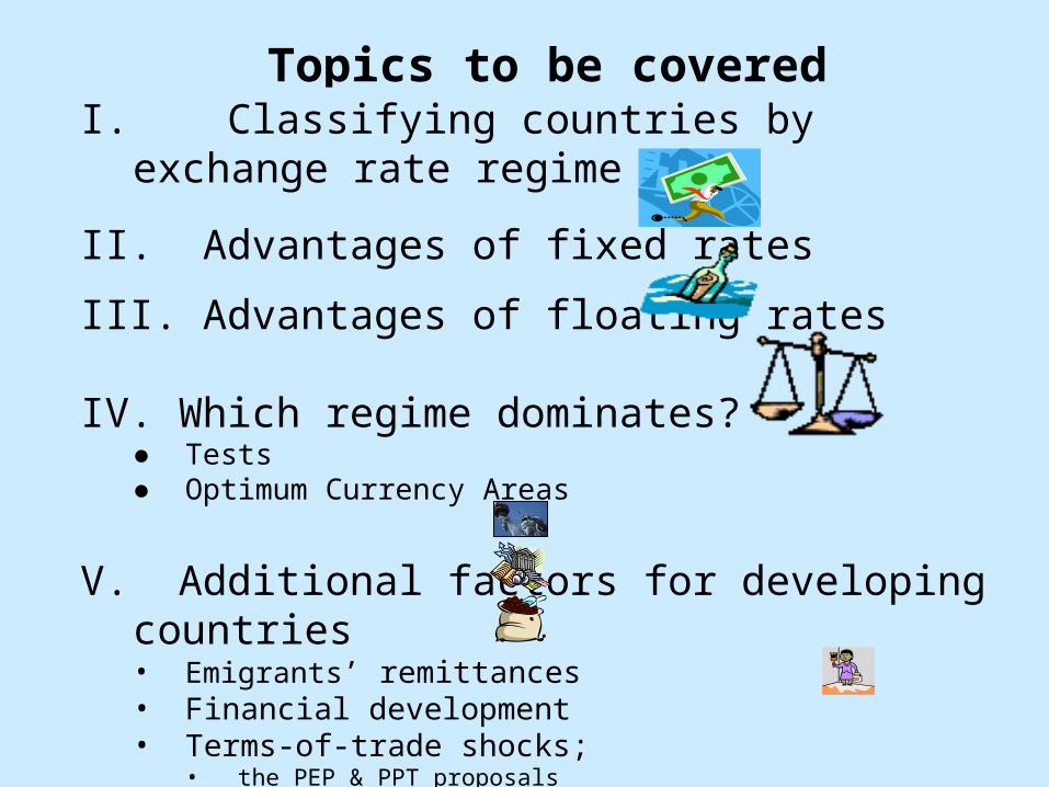
Continuum of exchange rate regimes:From flexible to rigid

FLEXIBLE CORNER

1) Free float 2) Managed float

INTERMEDIATE REGIMES

3) Target zone/band 4) Basket peg

5) Crawling peg 6) Adjustable peg

FIXED CORNER

7) Currency board 8) Dollarization

9) Monetary union

• Many countries that say they float, in fact intervene heavily in the foreign exchange market. [1]

• Many countries that say they fix, in fact devalue when trouble arises. [2]

• Many countries that say they target a basket of major currencies in fact fiddle with the weights. [3]

[1] “Fear of floating” -- Calvo & Reinhart (2001, 2002); Reinhart (2000).

[2] “The mirage of fixed exchange rates” -- Obstfeld & Rogoff (1995).

[3] Parameters kept secret -- Frankel, Schmukler & Servén (2000).

De jure regime de factoas is by now well-known

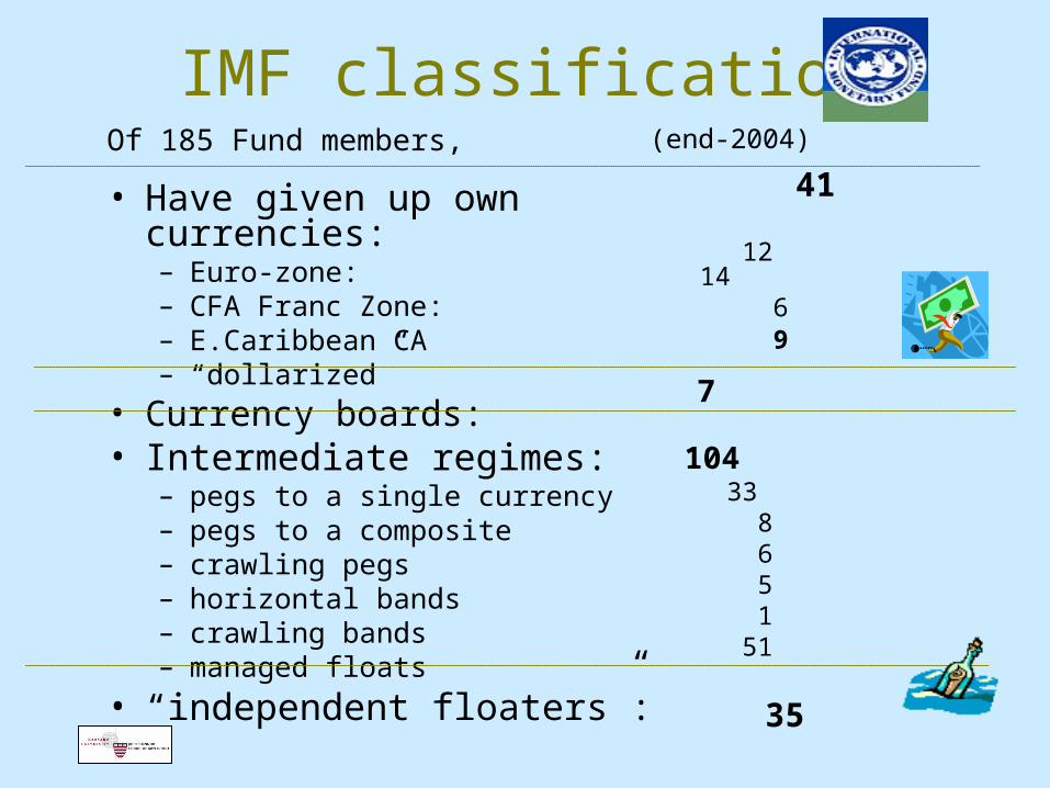
IMF classificationOf 185 Fund members,

• Have given up own currencies:– Euro-zone:– CFA Franc Zone:– E.Caribbean CA– “dollarized”

• Currency boards:

• Intermediate regimes:– pegs to a single currency– pegs to a composite– crawling pegs– horizontal bands– crawling bands– managed floats

• “independent floaters”:

(end-2004)

41

12 14

6 9

7 104

33 8 6 5 1 51

35

Schemes for de facto classification

• have themselves been divided into two classifications, viewed as:– “mixed de jure-de facto classifications,

because the self-declared regimes are adjusted

by the devisers for anomalies.”– Vs. “pure de facto classifications because…

assignment of regimes is based solely on statistical algorithms….”

-- Tavlas, Dellas & Stockman (2006).

Pure de facto classification schemes

1. Method to estimate degree of flexibility:• Calvo & Reinhart (2002) : var (exchange rate) vs. var (reserves).• Levy-Yeyati & Sturzenegger (2005): cluster analysis based on

variability of Δ exchange rates vs. variability of Δ reserves.

2. Method to estimate implicit basket weights: Regress Δ value of local currency against Δ values of major currencies. Frankel & Wei (1993, 95, 2007), Bénassy-Quéré (1999), B-Q et al (2004).

• Close fit => a peg. • Coefficient of 1 on $ => $ peg.

Or on other currencies => basket peg.• Example of China, post 7/2005.

3. Synthesis method: F & Wei (2008), F & Xie (2010) .

The de facto schemes do not agree

• That de facto schemes to classify exchange rate regimes differ from the IMF’s previous de jure classification is by now well-known.

• It is less well-known that the de facto schemes also do not agree with each other !

Professor Jeffrey Frankel

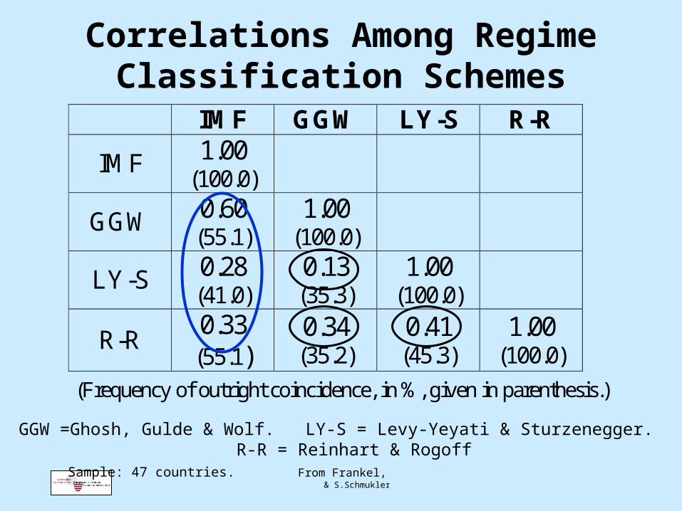
Correlations Among Regime Classification Schemes

Sample: 47 countries. From Frankel, ADB, 2004. Table 3, prepared by M. Halac & S.Schmukler.

IMF GGW LY-S R-R

IMF 1.00 (100.0)

GGW 0.60 (55.1)

1.00 (100.0)

LY-S 0.28 (41.0)

0.13 (35.3)

1.00 (100.0)

R-R 0.33 (55.1)

0.34 (35.2)

0.41 (45.3)

1.00 (100.0)

(Frequency of outright coincidence, in %, given in parenthesis.)

GGW =Ghosh, Gulde & Wolf. LY-S = Levy-Yeyati & Sturzenegger. R-R = Reinhart & Rogoff

Professor Jeffrey Frankel

II. Advantages of fixed rates

1) Encourage trade <= lower exchange risk. • In theory, can hedge risk. But costs of hedging:

missing markets, transactions costs, and risk premia.

• Empirical: Exchange rate volatility ↑ => trade ↓ ?

Time-series evidence showed little effect. But more in: - Cross-section evidence,

especially small & less developed countries.- Borders, e.g., Canada-US:

McCallum-Helliwell (1995-98); Engel-Rogers (1996).

- Currency unions: Rose (2000).

Professor Jeffrey Frankel

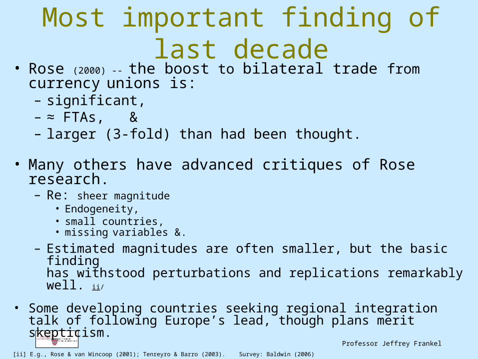
Most important finding of last decade• Rose (2000) -- the boost to bilateral trade from currency unions is:

– significant, – ≈ FTAs, & – larger (3-fold) than had been thought.

• Many others have advanced critiques of Rose research.– Re: sheer magnitude

• Endogeneity, • small countries, • missing variables &.

– Estimated magnitudes are often smaller, but the basic finding has withstood perturbations and replications remarkably well. ii/

• Some developing countries seeking regional integration talk of following Europe’s lead, though plans merit skepticism.

[ii] E.g., Rose & van Wincoop (2001); Tenreyro & Barro (2003). Survey: Baldwin (2006)

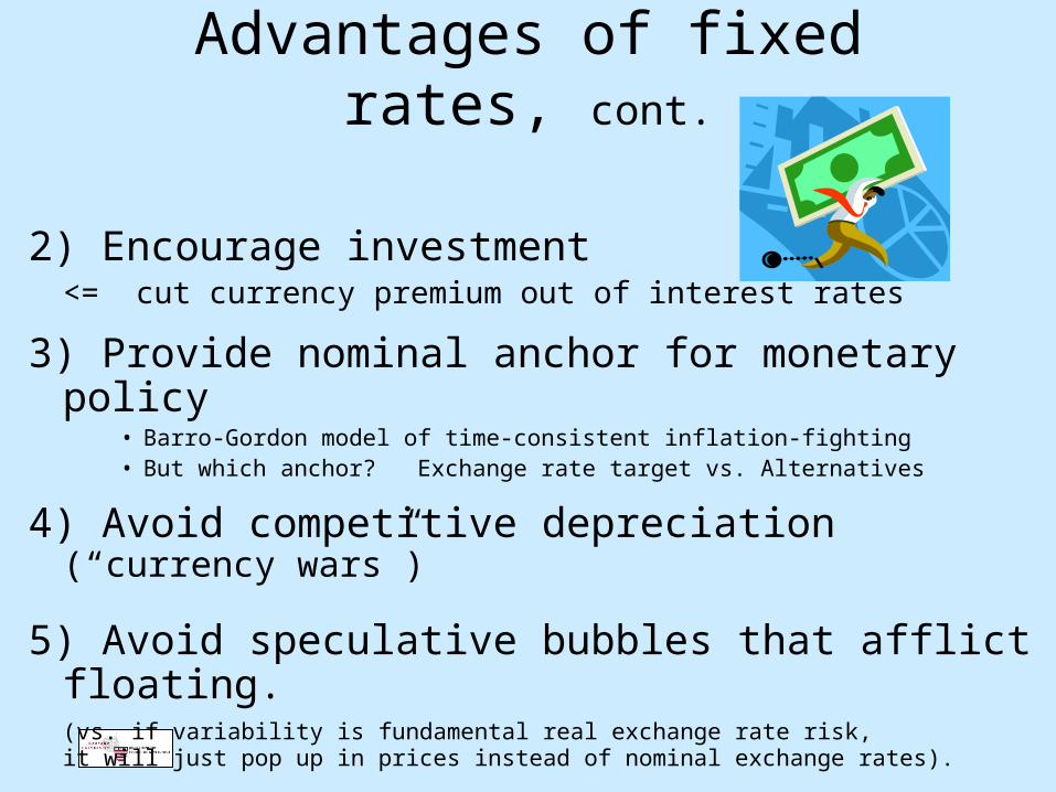
Advantages of fixed rates, cont.

2) Encourage investment <= cut currency premium out of interest rates

3) Provide nominal anchor for monetary policy• Barro-Gordon model of time-consistent inflation-fighting• But which anchor? Exchange rate target vs. Alternatives

4) Avoid competitive depreciation (“currency wars”)

5) Avoid speculative bubbles that afflict floating. (vs. if variability is fundamental real exchange rate risk, it will just pop up in prices instead of nominal exchange rates).

Professor Jeffrey Frankel

III. Advantages of floating rates

1. Monetary independence

2. Automatic adjustment to trade shocks

3. Retain seigniorage

4. Retain Lender of Last Resort ability

5. Avoiding crashes that hit pegged rates. (This is an advantage especially if origin of speculative attacks is multiple equilibria, not fundamentals.)

Professor Jeffrey Frankel

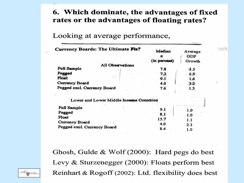
IV. Which dominate: advantages of fixing or advantages of floating?

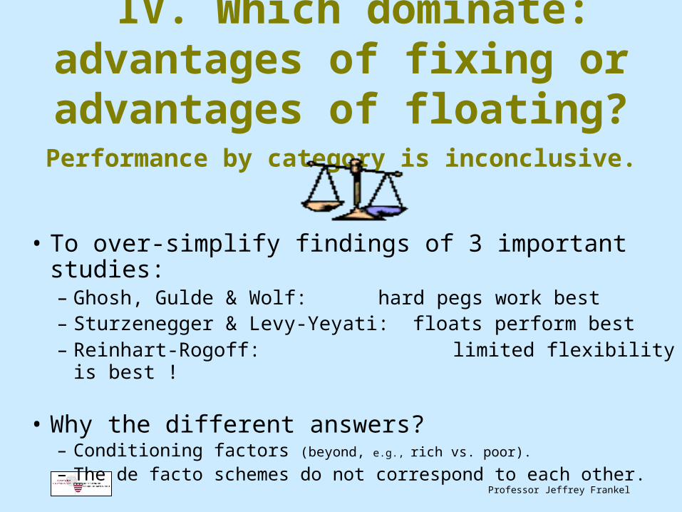
Performance by category is inconclusive.

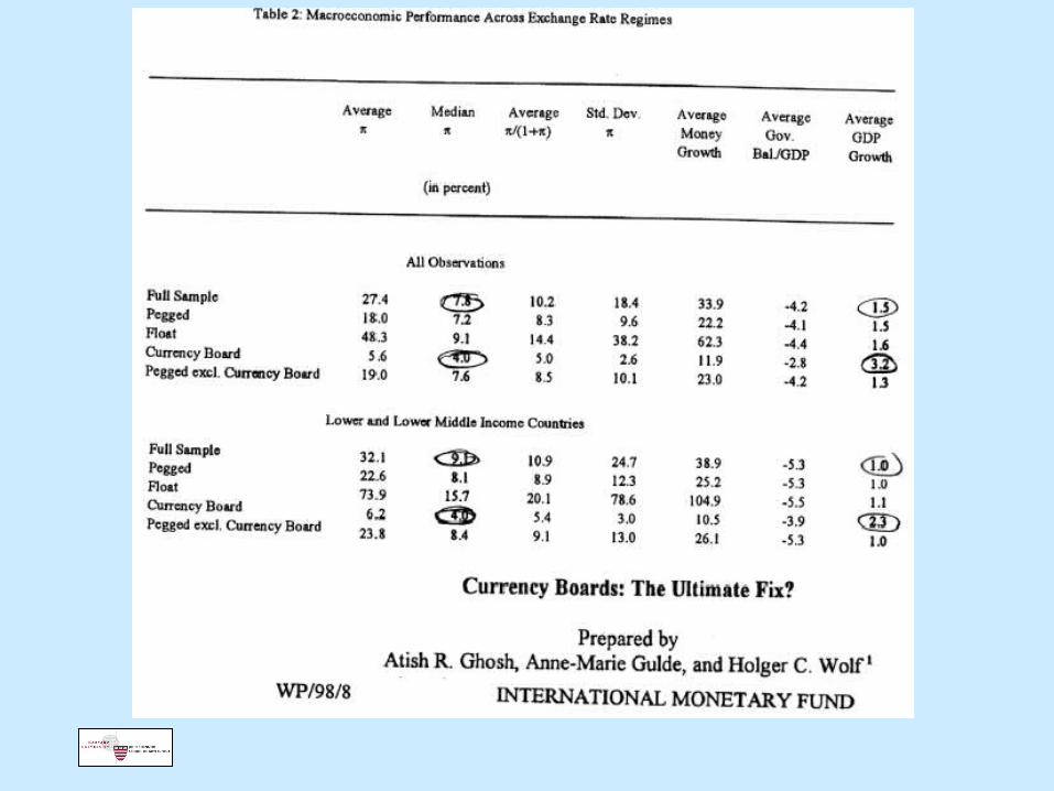
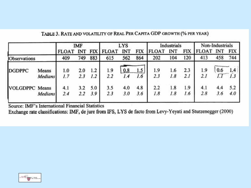
• To over-simplify findings of 3 important studies: – Ghosh, Gulde & Wolf: hard pegs work best– Sturzenegger & Levy-Yeyati: floats perform best– Reinhart-Rogoff: limited flexibility is best !

• Why the different answers? – Conditioning factors (beyond, e.g., rich vs. poor).

– The de facto schemes do not correspond to each other.

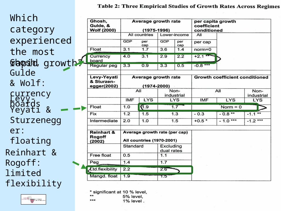
Which category experienced the most rapid growth?

Levy-Yeyati & Sturzenegger: floating

Reinhart & Rogoff:limited flexibility

Ghosh, Gulde & Wolf: currency boards

Which dominate: advantages of fixing or advantages of floating?

Answer depends on circumstances, of course:

No one exchange rate regime is rightfor all countries or all times.

• Traditional criteria for choosing - Optimum Currency Area. Focus is on trade and stabilization of business cycle.

• 1990s criteria for choosing – Focus is on financial markets and stabilization of speculation.

Professor Jeffrey Frankel

Optimum Currency Area Theory (OCA)

Broad definition: An optimum currency area is a region

that should have its own currency and own monetary policy.

This definition can be given more content:

An OCA can be defined as: a region that is neither so small and open that it would be better off pegging its currency to a neighbor, nor so large that it would be better off splitting into sub-regions with different currencies.

Professor Jeffrey Frankel

Optimum Currency Area criteria for fixing exchange rate:

• Small size and openness– because then advantages of fixing are large.

• Symmetry of shocks– because then giving up monetary independence is a small loss.

• Labor mobility– because then it is possible to adjust to shocks even without

ability to expand money, cut interest rates or devalue.

• Fiscal transfers in a federal system– because then consumption is cushioned in a downturn.

Professor Jeffrey Frankel

Some evidence on currency unions

Endogeneity of OCA criteria:

• Trade responds positively to currency regime -- Rose (2000)

• A pair’s cyclical correlation rises too(rather than falling, as under Eichengreen-Krugman hypothesis)

• Implication: members of a monetary union may meet OCA criteria better ex post than ex ante.

-- Frankel & Rose (1996)

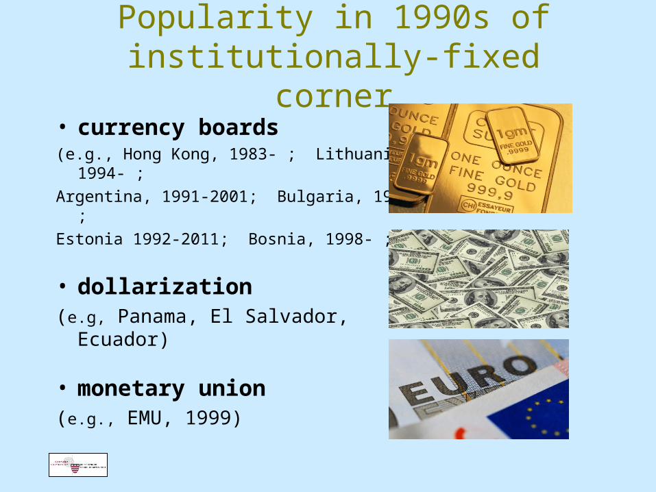
Popularity in 1990s ofinstitutionally-fixed corner

• currency boards (e.g., Hong Kong, 1983- ; Lithuania, 1994- ;

Argentina, 1991-2001; Bulgaria, 1997- ;

Estonia 1992-2011; Bosnia, 1998- ; …)

• dollarization (e.g, Panama, El Salvador, Ecuador)

• monetary union (e.g., EMU, 1999)

1990’s criteria for the firm-fix cornersuiting candidates for currency boards or union (e.g. Calvo)

Regarding credibility:

• a desperate need to import monetary stability, due to: history of hyperinflation,absence of credible public institutions, location in a dangerous neighborhood, orlarge exposure to nervous international investors

• a desire for close integration with a particular neighbor or trading partner

Regarding other “initial conditions”:• an already-high level of private dollarization• high pass-through to import prices• access to an adequate level of reserves • the rule of law.

Professor Jeffrey Frankel

V. Three additional considerations, particularly relevant

to developing countries

• (i) Emigrants’ remittances

• (ii) Level of financial development

• (iii) Supply shocks, especially: – External terms of trade shocks

and the proposal for Product Price Targeting PPT

I would like to add another criterionto the traditional OCA list:

Cyclically-stabilizing emigrants’ remittances.

• If country S has sent immigrants to country H, are their remittances correlated with the differential in growth or employment in S versus H?

• Apparently yes. (Frankel, “Are Bilateral Remittances Countercyclical?” 2011)

• This strengthens the case for S pegging to H.

• Why? It helps stabilize S’s current account even when S has given up ability to devalue.

Professor Jeffrey Frankel

(ii) Level of financial development Aghion, Bacchetta, Ranciere & Rogoff (2005)

– Fixed rates are better for countries at low levels of financial development: because markets are thin => benefits of accommodating real shocks are outweighed by costs of financial shocks.

– When financial markets develop, exchange flexibility becomes more attractive.

– Estimated threshold: Private Credit/GDP > 40%.

Professor Jeffrey Frankel

Level of financial development, cont. Husain, Mody & Rogoff (2005)

• For poor countries with low capital mobility, pegs work

– in the sense of being more durable

– & delivering low inflation

• For richer & more financially developed countries, flexible rates work better– in the sense of being more durable

– & delivering higher growth without inflation

Professor Jeffrey Frankel

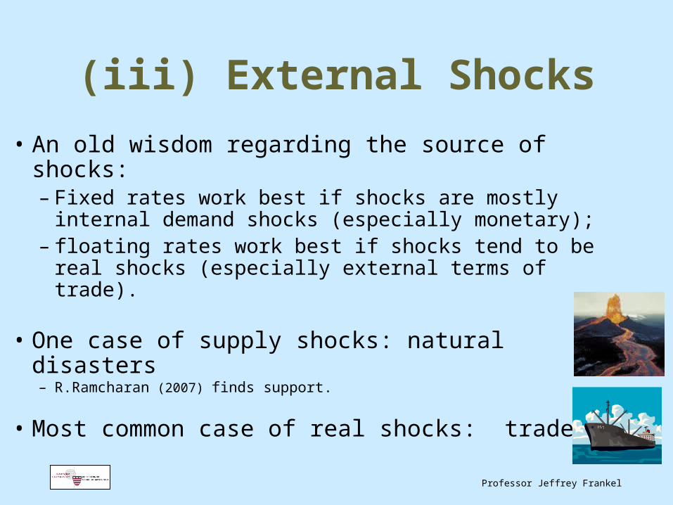
(iii) External Shocks

• An old wisdom regarding the source of shocks:– Fixed rates work best if shocks are mostly internal

demand shocks (especially monetary); – floating rates work best if shocks tend to be real

shocks (especially external terms of trade).

• One case of supply shocks: natural disasters– R.Ramcharan (2007) finds support.

• Most common case of real shocks: trade

Professor Jeffrey Frankel

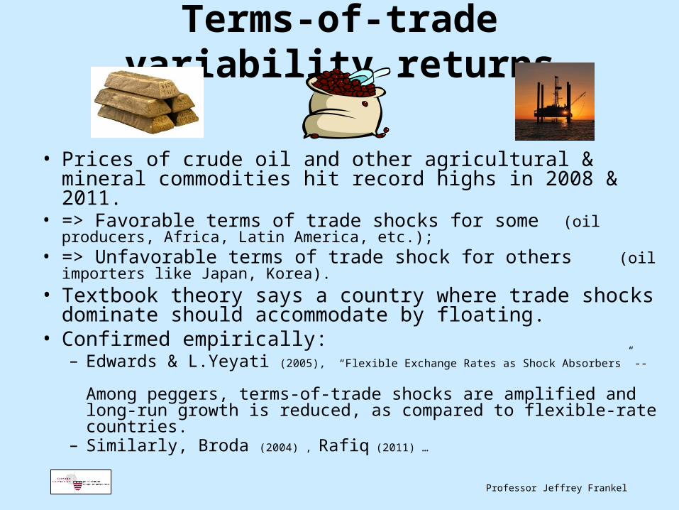
Terms-of-trade variability returns

• Prices of crude oil and other agricultural & mineral commodities hit record highs in 2008 & 2011.

• => Favorable terms of trade shocks for some (oil producers, Africa, Latin America, etc.);

• => Unfavorable terms of trade shock for others (oil importers like Japan, Korea).

• Textbook theory says a country where trade shocks dominate should accommodate by floating.

• Confirmed empirically:– Edwards & L.Yeyati (2005), “Flexible Exchange Rates as Shock Absorbers” --

Among peggers, terms-of-trade shocks are amplified and long-run growth is reduced, as compared to flexible-rate countries.

– Similarly, Broda (2004) , Rafiq (2011) …

Professor Jeffrey Frankel

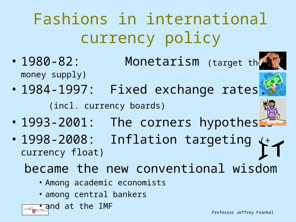
Fashions in international currency policy

• 1980-82: Monetarism (target the money supply)

• 1984-1997: Fixed exchange rates (incl. currency boards)

• 1993-2001: The corners hypothesis• 1998-2008: Inflation targeting (+ currency float)

became the new conventional wisdom• Among academic economists

• among central bankers

• and at the IMF

Professor Jeffrey Frankel

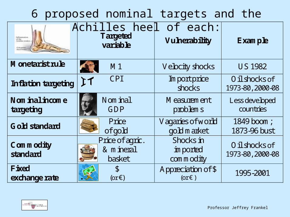
6 proposed nominal targets and the Achilles heel of each:

Targeted variable

Vulnerability Example

Monetarist rule

M1 Velocity shocks US 1982

Inflation targeting CPI

Import price

shocks Oil shocks of

1973-80, 2000-08

Nominal income targeting

Nominal GDP

Measurement problems

Less developed countries

Gold standard Price

of gold Vagaries of world

gold market 1849 boom; 1873-96 bust

Commodity standard

Price of agric. & mineral

basket

Shocks in imported

commodity

Oil shocks of 1973-80, 2000-08

Fixed exchange rate

$ (or €)

Appreciation of $ (or € ) 1995-2001

Professor Jeffrey Frankel

Inflation Targeting has been the reigning orthodoxy.

• Flexible inflation targeting ≡“Have a LR target for inflation, and be transparent.”

Who could disagree?

• But define IT as setting yearly CPI targets, to the exclusion of

• asset prices

• exchange rates

• export commodity prices.

• Some reexamination is warranted, in light of 2008-2012.

Professor Jeffrey Frankel

• The shocks of 2008-2012 showed The shocks of 2008-2012 showed disadvantages to Inflation Targetingdisadvantages to Inflation Targeting ,,– analogously to how the EM crises of the 1994-2001analogously to how the EM crises of the 1994-2001

showed disadvantages of exchange rate targeting.showed disadvantages of exchange rate targeting.

• One disadvantage of IT: One disadvantage of IT: no response to asset price bubbles.no response to asset price bubbles.

• Another disadvantageAnother disadvantage::

– It gives the wrong answer in case of trade shocks:It gives the wrong answer in case of trade shocks:• E.g., it says to tighten money & appreciate

in response to a rise in oil import prices; • It does not allow monetary tightening

& appreciation in response to a rise in world prices of export commodities.

• That is backwards.

Professor Jeffrey Frankel

Proposal for Product Price Targeting

Intended for countries with volatile terms of trade, e.g., those specialized in commodities.

The authorities stabilize the currency in terms of an index of product prices, such as the GDP deflator, (a basket that gives weight to prices of its commodity exports),

rather than to the CPI (which gives weight to imports).

The regime combines the best of both worlds:

(i) The advantage of automatic accommodation to terms of trade shocks, together with

(ii) the advantages of a nominal anchor.

PPT

Professor Jeffrey Frankel

Why is PPT better than CPI-targetingfor countries with volatile terms of trade?

Better response to adverse terms of trade shocks:

• If the $ price of the export commodity goes up, PPT says to tighten monetary policy enough to appreciate currency. – Right response. (E.g., Gulf currencies in 2007-08.)

• If the $ price of imported commodity goes up, CPI target says to tighten monetary policy enough to appreciate currency. – Wrong response. (E.g., oil-importers in 2007-08.)

– => CPI targeting gets it backwards.

PPT

VI. Intermediate exchange rate regimes

and the corners hypothesis

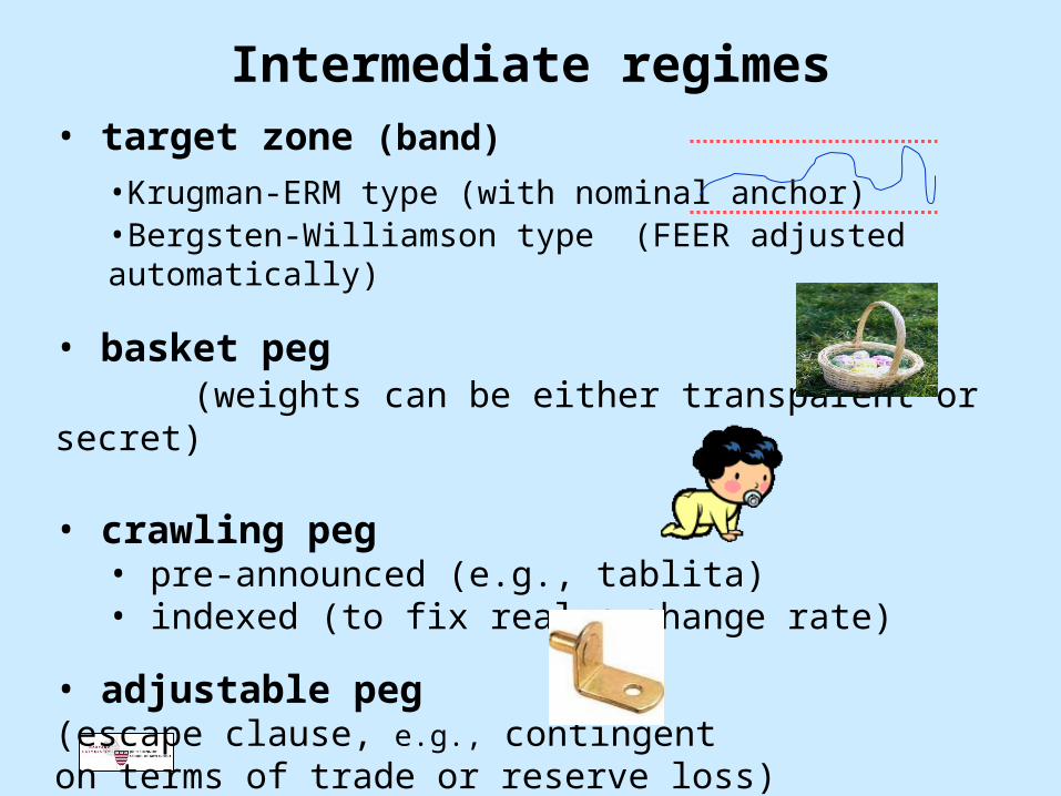
Intermediate regimes• target zone (band)

•Krugman-ERM type (with nominal anchor)•Bergsten-Williamson type (FEER adjusted automatically)

• basket peg (weights can be either transparent or secret)

• crawling peg• pre-announced (e.g., tablita) • indexed (to fix real exchange rate)

• adjustable peg (escape clause, e.g., contingenton terms of trade or reserve loss)

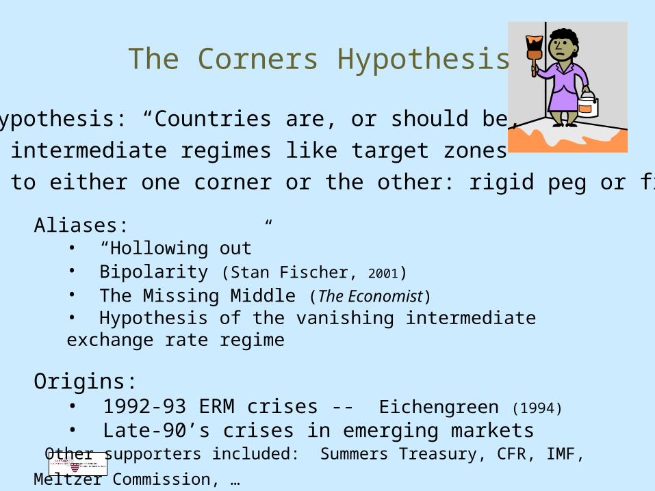
Aliases:• “Hollowing out”• Bipolarity (Stan Fischer, 2001)• The Missing Middle (The Economist)• Hypothesis of the vanishing intermediate exchange rate regime

Origins:• 1992-93 ERM crises -- Eichengreen (1994)

• Late-90’s crises in emerging markets Other supporters included: Summers Treasury, CFR, IMF, Meltzer Commission, …

The Corners Hypothesis

• The hypothesis: “Countries are, or should be,

abandoning intermediate regimes like target zones

and moving to either one corner or the other: rigid peg or free float.

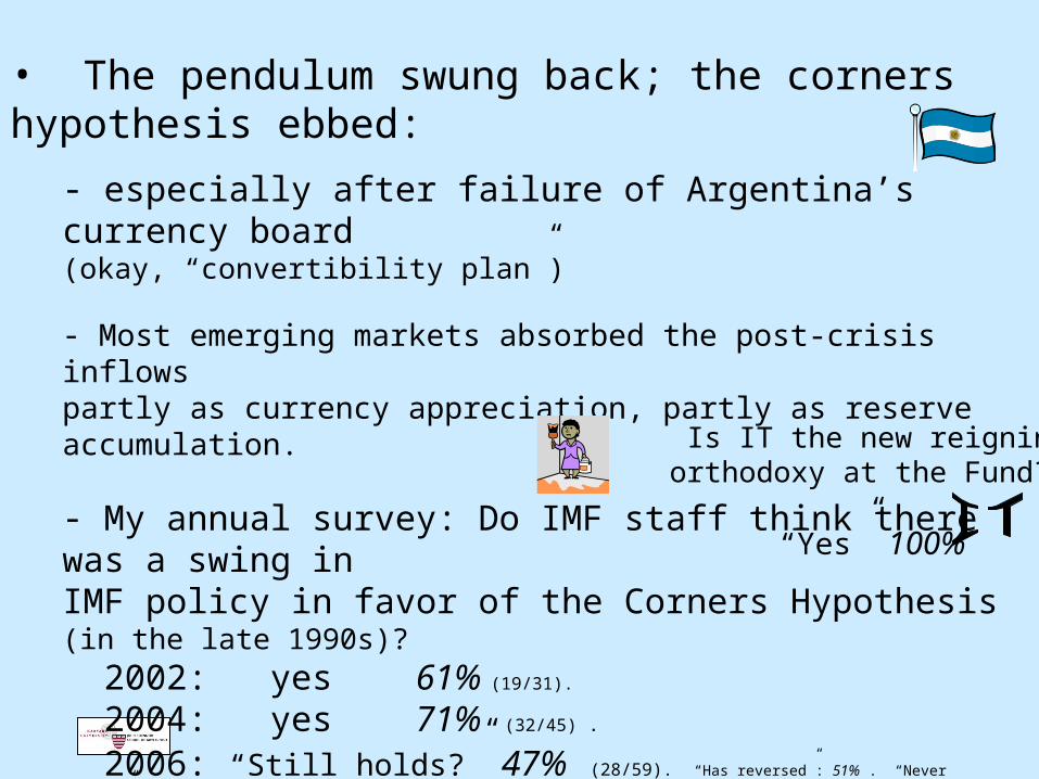
• The pendulum swung back; the corners hypothesis ebbed:

- especially after failure of Argentina’s currency board (okay, “convertibility plan”)

- Most emerging markets absorbed the post-crisis inflows partly as currency appreciation, partly as reserve accumulation.

- My annual survey: Do IMF staff think there was a swing in IMF policy in favor of the Corners Hypothesis (in the late 1990s)?

2002: yes 61% (19/31).

2004: yes 71% (32/45) .

2006: “Still holds?” 47% (28/59). “Has reversed”: 51% . “Never serious”: 2%

2007: 43% (16/34) “Has reversed”: 49% . “Never serious”: 8% 63% 2008: 50% (16/34) “Has reversed”: 48% . “Never serious”: 2% 72% 2010: 0% (0/24). 58% 2011: 97%

Do you personally believe in IT? 38%

Is IT the new reigning orthodoxy at the Fund?

“Yes” 100%

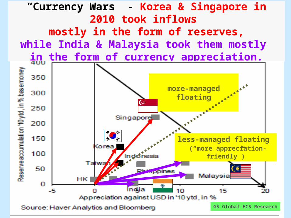
“Currency Wars” - Korea & Singapore in 2010 took inflows

mostly in the form of reserves,while India & Malaysia took them mostly

in the form of currency appreciation.

GS Global ECS Research

less-managed floating (“more appreciation-friendly”)

more-managed floating

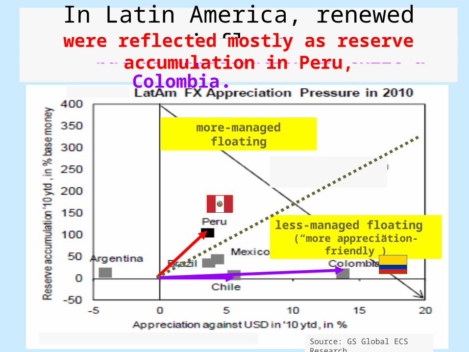
In Latin America, renewed inflows

less-managed floating (“more appreciation-friendly”)

more-managed floating

Source: GS Global ECS Research

but as appreciation in Chile & Colombia. were reflected mostly as reserve accumulation in Peru,

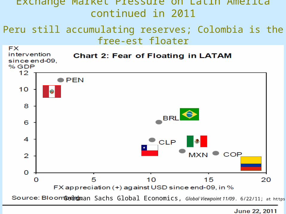
Exchange Market Pressure on Latin America continued in 2011

Peru still accumulating reserves; Colombia is the free-est floater

Goldman Sachs Global Economics, Global Viewpoint 11/09. 6/22/11; at https://360.gs.com

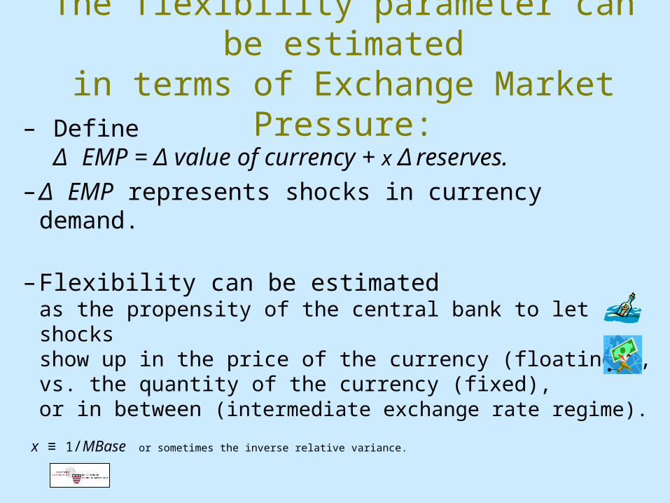
The flexibility parameter can be estimatedin terms of Exchange Market Pressure:

– Define Δ EMP = Δ value of currency + x Δ reserves.

– Δ EMP represents shocks in currency demand.

– Flexibility can be estimated as the propensity of the central bank to let shocks show up in the price of the currency (floating) ,vs. the quantity of the currency (fixed), or in between (intermediate exchange rate regime).

x ≡ 1/MBase or sometimes the inverse relative variance.

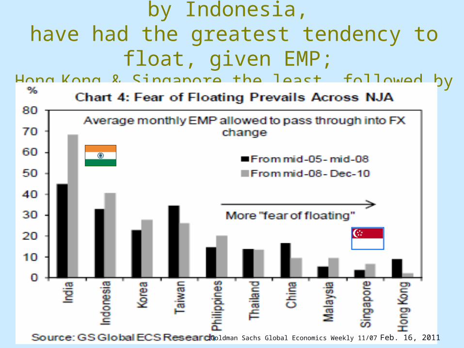
In Asia since 2008, India, followed by Indonesia, have had the greatest tendency to float, given EMP;

Hong Kong & Singapore the least, followed by Malaysia & China.

Goldman Sachs Global Economics Weekly 11/07 Feb. 16, 2011

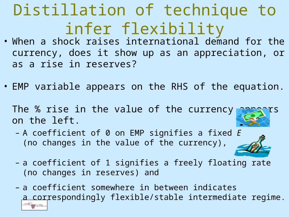
Distillation of technique to infer flexibility• When a shock raises international demand for the currency,

does it show up as an appreciation, or as a rise in reserves?

• EMP variable appears on the RHS of the equation. The % rise in the value of the currency appears on the left. – A coefficient of 0 on EMP signifies a fixed E

(no changes in the value of the currency),

– a coefficient of 1 signifies a freely floating rate (no changes in reserves) and

– a coefficient somewhere in between indicates a correspondingly flexible/stable intermediate regime.

Appendix 1

On the RMB

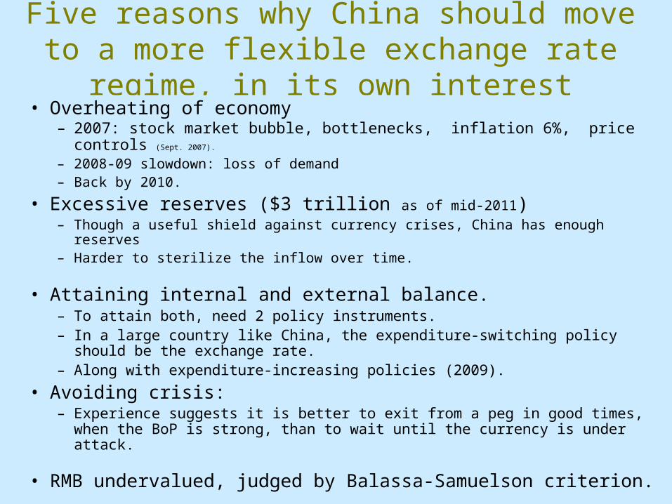
Five reasons why China should move to a more flexible exchange rate regime, in its own interest

• Overheating of economy– 2007: stock market bubble, bottlenecks, inflation 6%, price controls (Sept. 2007).

– 2008-09 slowdown: loss of demand– Back by 2010.

• Excessive reserves ($3 trillion as of mid-2011)– Though a useful shield against currency crises, China has enough reserves– Harder to sterilize the inflow over time.

• Attaining internal and external balance.– To attain both, need 2 policy instruments. – In a large country like China, the expenditure-switching policy

should be the exchange rate.– Along with expenditure-increasing policies (2009).

• Avoiding crisis: – Experience suggests it is better to exit from a peg in good times,

when the BoP is strong, than to wait until the currency is under attack.

• RMB undervalued, judged by Balassa-Samuelson criterion.

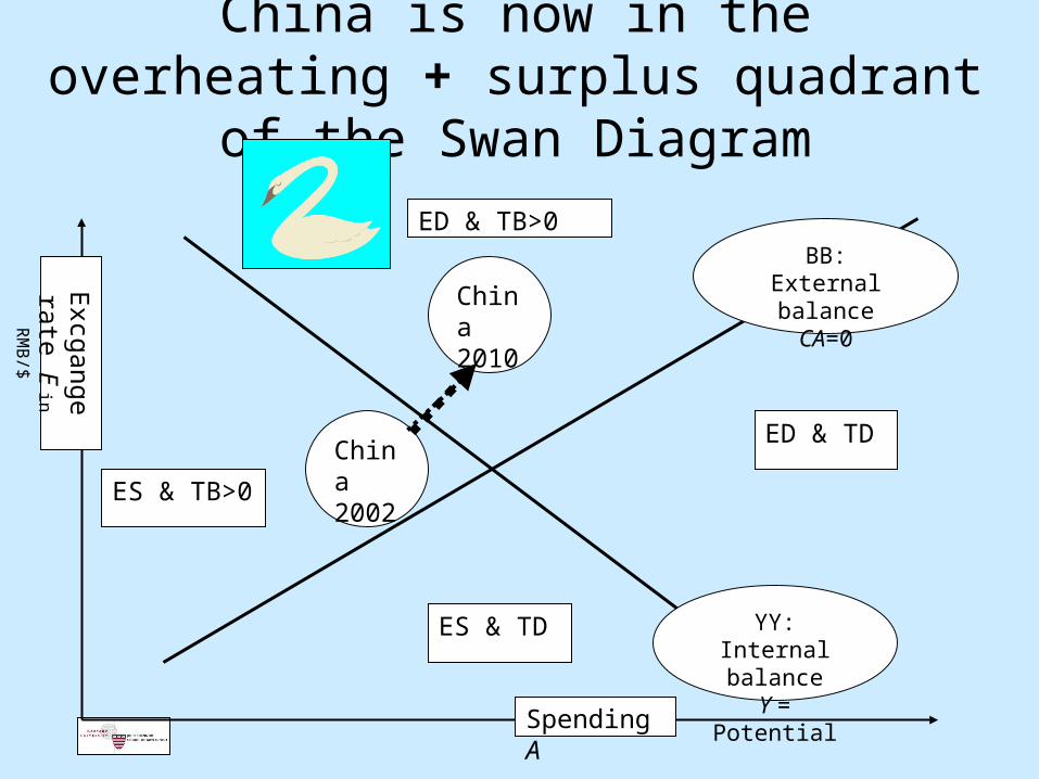
China is now in the overheating + surplus quadrant of the Swan Diagram

Excgange rate E

in R

MB

/$

YY:Internal balance

Y = Potential

ED & TD

ES & TD

ES & TB>0

China2010

BB:External balance

CA=0

China2002

ED & TB>0

Spending A

How should changes in real exchange rate, when necessary, be achieved?

• For a very small, open economy– advantages of keeping E fixed are large.– Adjustment may take place via prices instead– Example: Hong Kong

• For a large economy like China, it makes more sense to adjust E than to adjust prices

What would new regime be?

• No need for pure float. • China is an example of why the Corners

Hypothesis is wrong• Band or target zone may be best• With what as anchor?

– Advantage of dollar: simple and transparent– Advantage of basket: better diversification– Asia currently lacks a good anchor currency.

What about the currency reform announced in July 2005?

• Movements of effective exchange rate have been small,

vs. movement of $, € & ¥.

• China did not really adopt the regime it said:

basket peg (with cumulatable +/- .3% band)– De facto weight on $ still 100% in late 2005

– During 2007, weight had indeed shifted away from $;

– Appreciation of € explained appreciation of RMB against $.

– In mid-2008, RMB shifted back to a de facto $ peg again.

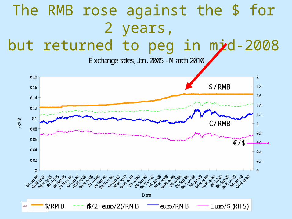
The RMB rose against the $ for 2 years, but returned to peg in mid-2008

Exchange rates, Jan. 2005 - March 2010

0

0.02

0.04

0.06

0.08

0.1

0.12

0.14

0.16

0.18

Date

/RM

B

0

0.2

0.4

0.6

0.8

1

1.2

1.4

1.6

1.8

2

$/ RMB ($/ 2+euro/ 2)/ RMB euro/ RMB Euro/ $ (RHS)

$/RMB

€/RMB

€/$

Appendix 2

Tables comparing economic performance of different regimes:

– Ghosh, Gulde & Wolf

– Sturzenegger & Levy-Yeyati

– Reinhart & Rogoff

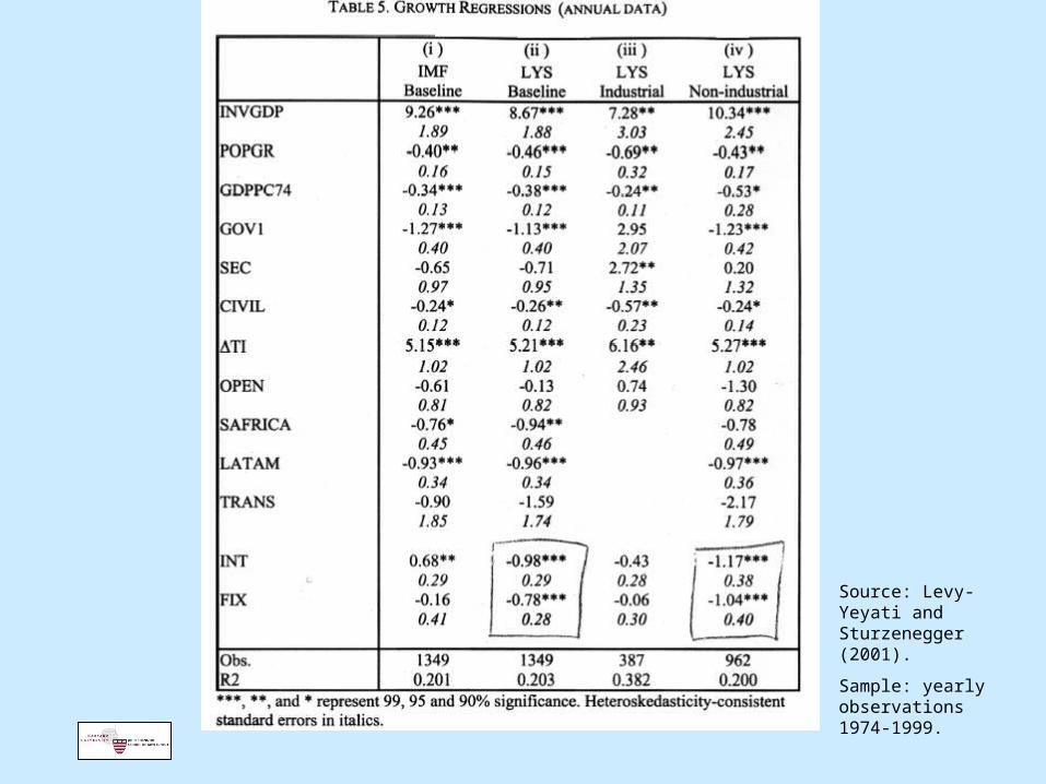
Source: Levy-Yeyati and Sturzenegger (2001).

Sample: yearly observations 1974-1999.

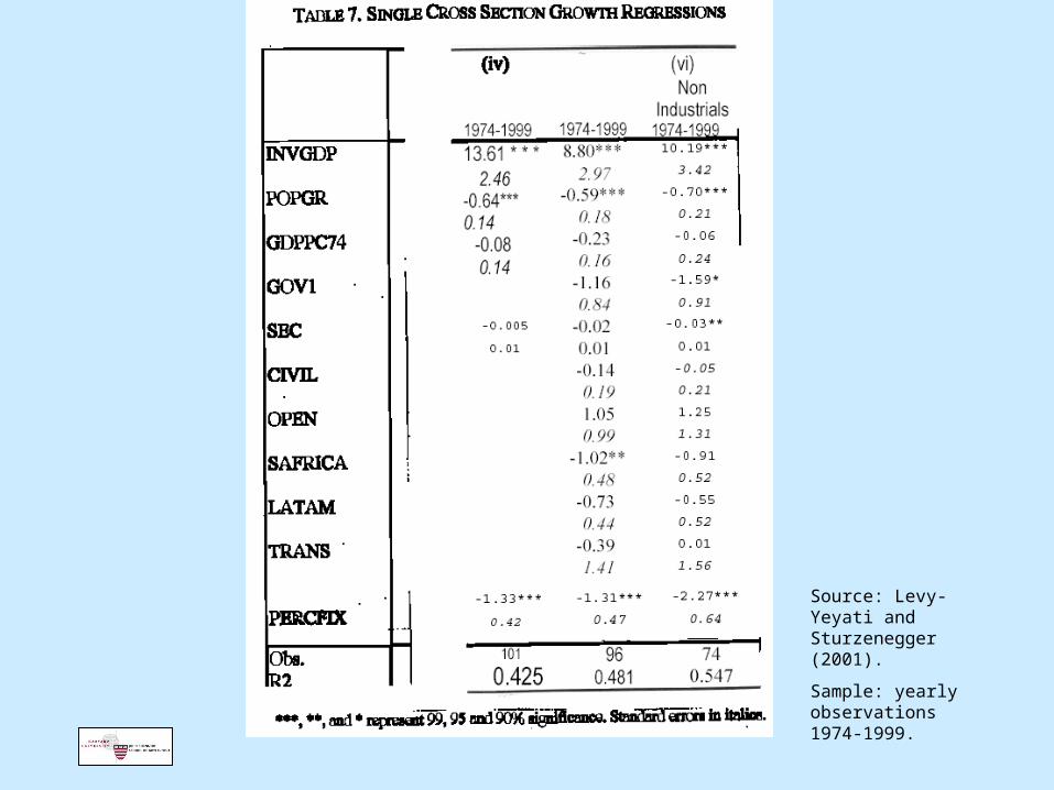
Source: Levy-Yeyati and Sturzenegger (2001).

Sample: yearly observations 1974-1999.

Appendix 3:The econometrics of estimatingde facto exchange rate regimes.

• Why do the various schemes for classifying countries by de facto exchange rate regimes give such different answers?

• Synthesis of the technique for estimating the anchor and the technique for estimating the degree of exchange rate flexibility.

Professor Jeffrey Frankel

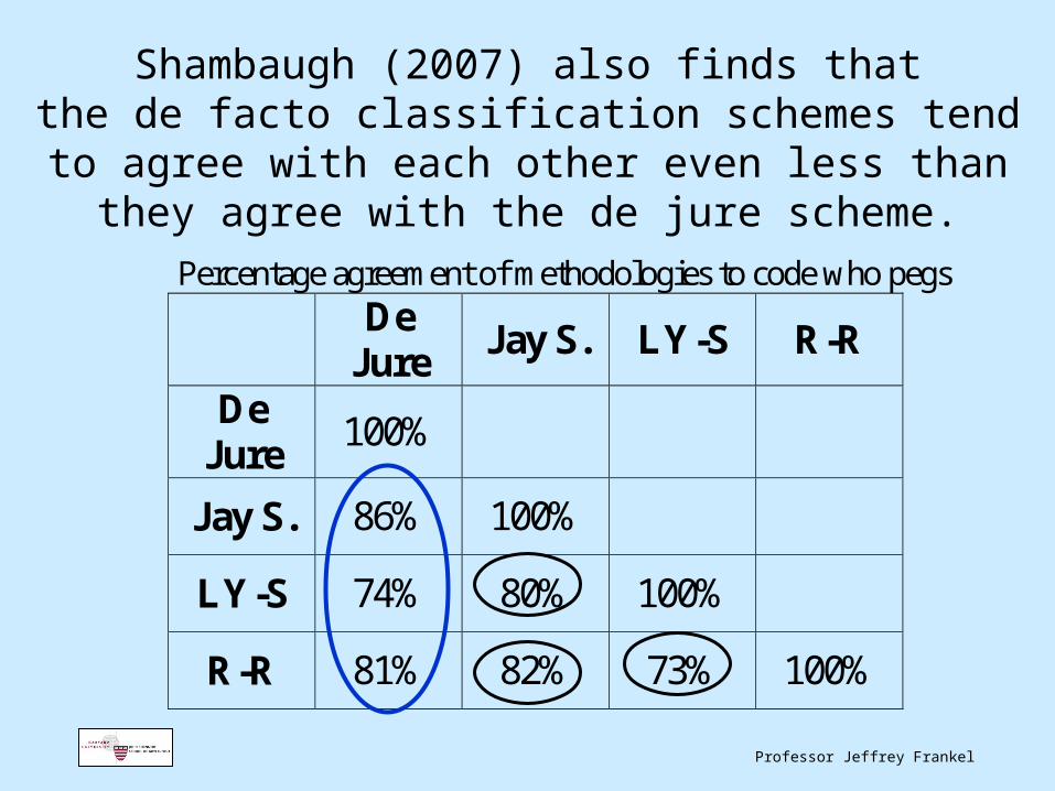
Shambaugh (2007) also finds thatthe de facto classification schemes tend to agree with each

other even less than they agree with the de jure scheme.

Percentage agreement of methodologies to code who pegs

De

Jure Jay S. LY-S R-R

De Jure

100%

Jay S.

86% 100%

LY-S

74% 80% 100%

R-R

81% 82% 73% 100%

Professor Jeffrey Frankel

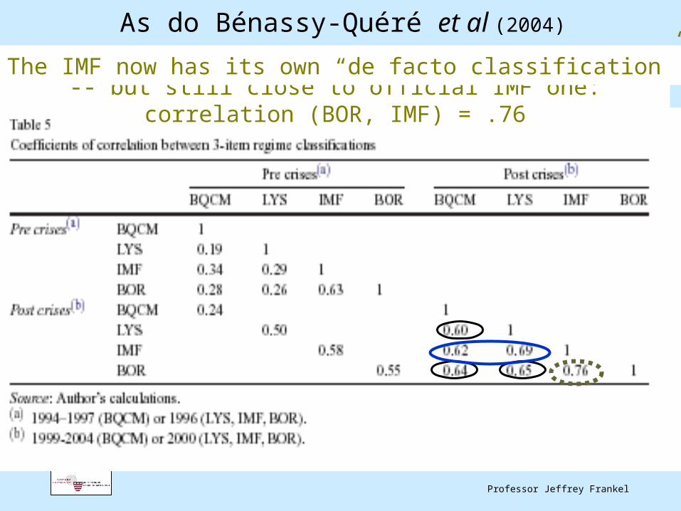
-- but still close to official IMF one: correlation (BOR, IMF) = .76

The IMF now has its own “de facto classification”

As do Bénassy-Quéré et al (2004)

Professor Jeffrey Frankel

Several things are wrong.Difficulty #1:

Attempts to infer statistically a currency’s flexibility from the variability of its exchange rate alone ignore that some countries experience greater shocks than others.

That problem can be addressed by comparing exchange rate variability to foreign exchange reserve variability:

Calvo & Reinhart (2002); Levy-Yeyati & Sturzenegger (2003, 2005).

What is wrong with the schemes for estimating

de facto exchange rate regimes, that they give such different answers?

Professor Jeffrey Frankel

Phrase this 1st approach in terms of Exchange Market Pressure:

• Define EMP = Δ value of currency + Δ reserves.– EMP represents shocks in currency demand.– Flexibility can be estimated

as the propensity of the central bank to let shocks show up in the price of the currency (floating) ,vs. the quantity of the currency (fixed), or in between (intermediate exchange rate regime).

Professor Jeffrey Frankel

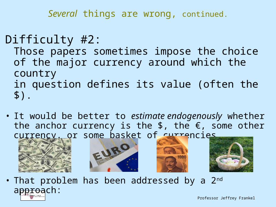
Several things are wrong, continued.

Difficulty #2: Those papers sometimes impose the choice of the major currency around which the country in question defines its value (often the $).

• It would be better to estimate endogenously whether the anchor currency is the $, the €, some other currency, or some basket of currencies.

• That problem has been addressed by a 2nd approach:

Professor Jeffrey Frankel

• Some currencies have basket anchors, often with some flexibility that can be captured either by a band (BBC) or

by leaning-against-the-wind intervention.

• Most basket peggers keep the weights secret. They want to preserve a degree of freedom from prying eyes, whether to pursue

– less de facto flexibility, as China, – or more, as with most others.

Professor Jeffrey Frankel

The 2nd approach in the de facto regime literature estimates implicit basket weights:

Regress Δvalue of local currency against Δ values of major currencies.

• First examples: Frankel (1993) and Frankel & Wei (1994, 95). • More: Bénassy-Quéré (1999), Ohno (1999), Frankel, Schmukler,

Servén & Fajnzylber (2001), Bénassy-Quéré, Coeuré, & Mignon (2004)….

• Example of China, post 7/05: – Eichengreen (2006), Shah, Zeileis & Patnaik (2005), Yamazaki (2006),

Ogawa (2006), Frankel-Wei (2006, 07), Frankel (2009)

– Findings: • RMB still pegged in 2005-06, with 95% weight on $.• Moved away from $ (weight on €) in 2007-08• Returned to $ peg in mid 2008. Left again in 2010.

Professor Jeffrey Frankel

Implicit basket weights method -- regress Δvalue of local currency against

Δ values of major currencies -- continued.

• Null Hypotheses: Close fit => a peg. • Coefficient of 1 on $ => $ peg.

• Or significant weights on other currencies => basket

peg.

• But if the test rejects tight basket peg, what is the Alternative Hypothesis?

Professor Jeffrey Frankel

Several things are wrong, continued.

Difficulty #3: The 2nd approach (inferring the anchor currency or basket) does not allow for flexibility around that anchor.

• Inferring de facto weights and inferring de facto flexibility are equally important,

• whereas most authors have hitherto done only one or the other.

Professor Jeffrey Frankel

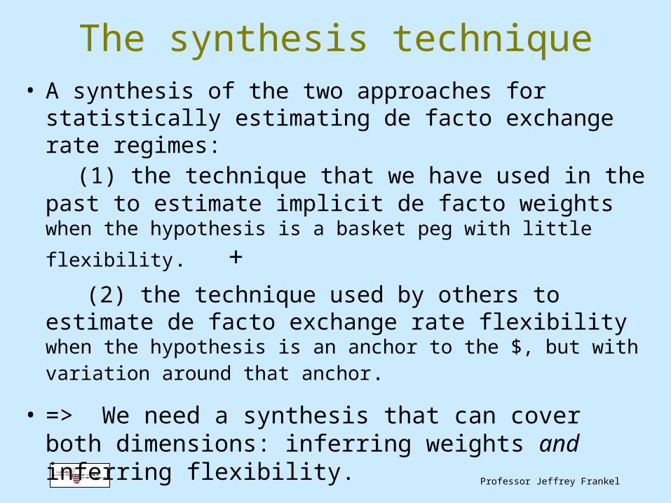
The synthesis technique• A synthesis of the two approaches for statistically

estimating de facto exchange rate regimes: (1) the technique that we have used in the past to estimate implicit de facto weights

when the hypothesis is a basket peg with little flexibility. +

(2) the technique used by others to estimate de facto exchange rate flexibility when the hypothesis is an anchor to

the $, but with variation around that anchor.

• => We need a synthesis that can cover both dimensions: inferring weights and inferring flexibility.

Professor Jeffrey Frankel

Several things are wrong, continued.

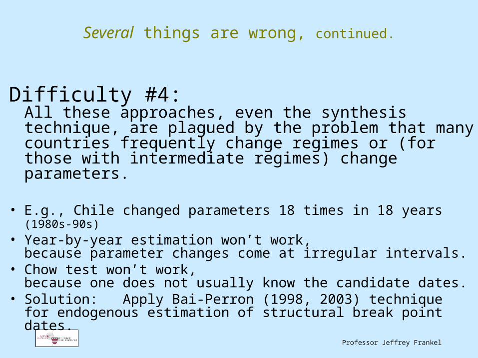
Difficulty #4: All these approaches, even the synthesis technique, are plagued by the problem that many countries frequently change regimes or (for those with intermediate regimes) change parameters.

• E.g., Chile changed parameters 18 times in 18 years (1980s-90s) • Year-by-year estimation won’t work,

because parameter changes come at irregular intervals.• Chow test won’t work,

because one does not usually know the candidate dates.• Solution: Apply Bai-Perron (1998, 2003) technique

for endogenous estimation of structural break point dates.

Professor Jeffrey Frankel

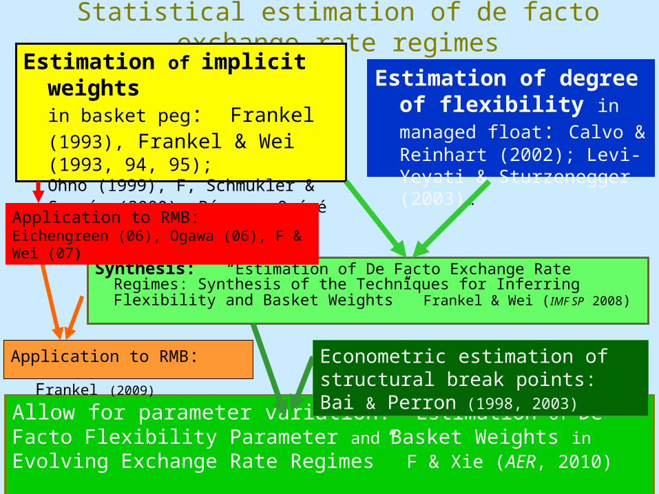
Statistical estimation of de facto exchange rate regimes

Synthesis: “Estimation of De Facto Exchange Rate Regimes: Synthesis of the Techniques for Inferring Flexibility and Basket Weights” Frankel & Wei (IMF SP 2008)

Estimation of implicit weights in basket peg: Frankel (1993), Frankel & Wei (1993, 94, 95); Ohno (1999), F, Schmukler & Servén (2000), Bénassy-Quéré (1999, 2006)…

Estimation of degree of flexibility in managed float: Calvo & Reinhart (2002); Levi-Yeyati & Sturzenegger (2003)…

Allow for parameter variation: “Estimation of De Facto Flexibility Parameter and Basket Weights in Evolving Exchange Rate Regimes” F & Xie (AER, 2010)

Application to RMB: Frankel (2009) Econometric estimation of structural break points: Bai & Perron (1998, 2003)

Application to RMB:Eichengreen (06), Ogawa (06), F & Wei (07)

Professor Jeffrey Frankel

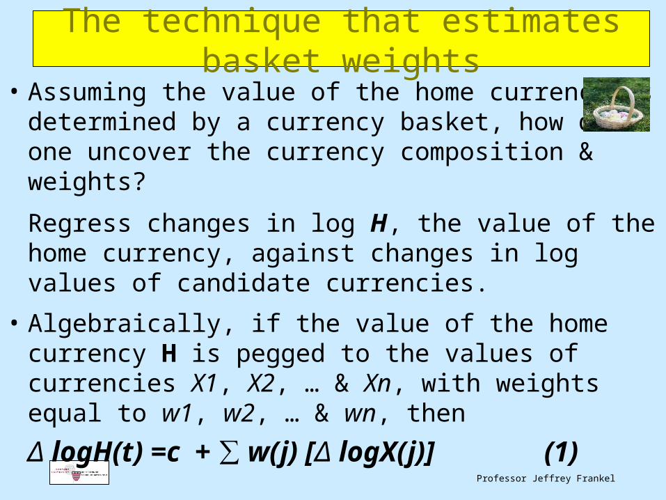
The technique that estimates basket weights

• Assuming the value of the home currency is determined by a currency basket, how does one uncover the currency composition & weights?

Regress changes in log H, the value of the home currency, against changes in log values of candidate currencies.

• Algebraically, if the value of the home currency H is pegged to the values of currencies X1, X2, … & Xn, with weights equal to w1, w2, … & wn, then

Δ logH(t) =c + ∑ w(j) [Δ logX(j)] (1)

Professor Jeffrey Frankel

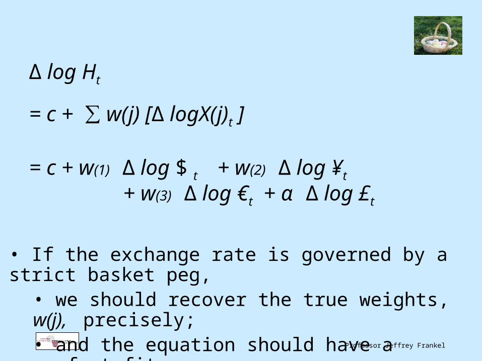
Δ log Ht

= c + ∑ w(j) [Δ logX(j)t ]

= c + w(1) Δ log $ t + w(2) Δ log ¥t

+ w(3) Δ log €t + α Δ log £t

• If the exchange rate is governed by a strict basket peg,• we should recover the true weights, w(j), precisely; • and the equation should have a perfect fit.

Professor Jeffrey Frankel

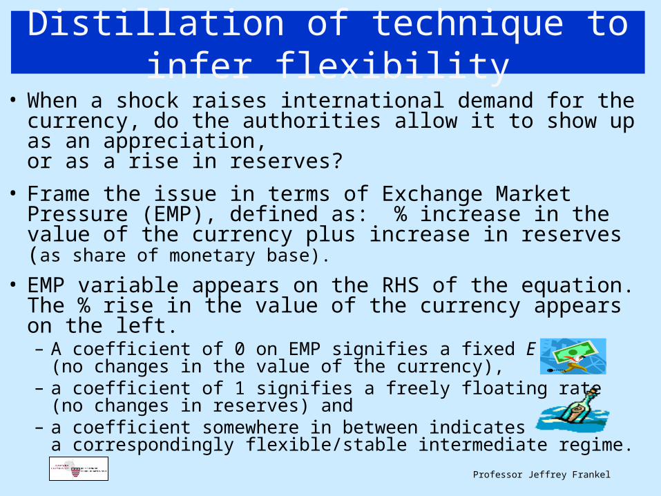
Distillation of technique to infer flexibility

• When a shock raises international demand for the currency, do the authorities allow it to show up as an appreciation, or as a rise in reserves?

• Frame the issue in terms of Exchange Market Pressure (EMP), defined as: % increase in the value of the currency plus increase in reserves (as share of monetary base).

• EMP variable appears on the RHS of the equation. The % rise in the value of the currency appears on the left. – A coefficient of 0 on EMP signifies a fixed E

(no changes in the value of the currency), – a coefficient of 1 signifies a freely floating rate

(no changes in reserves) and – a coefficient somewhere in between indicates

a correspondingly flexible/stable intermediate regime.

Professor Jeffrey Frankel

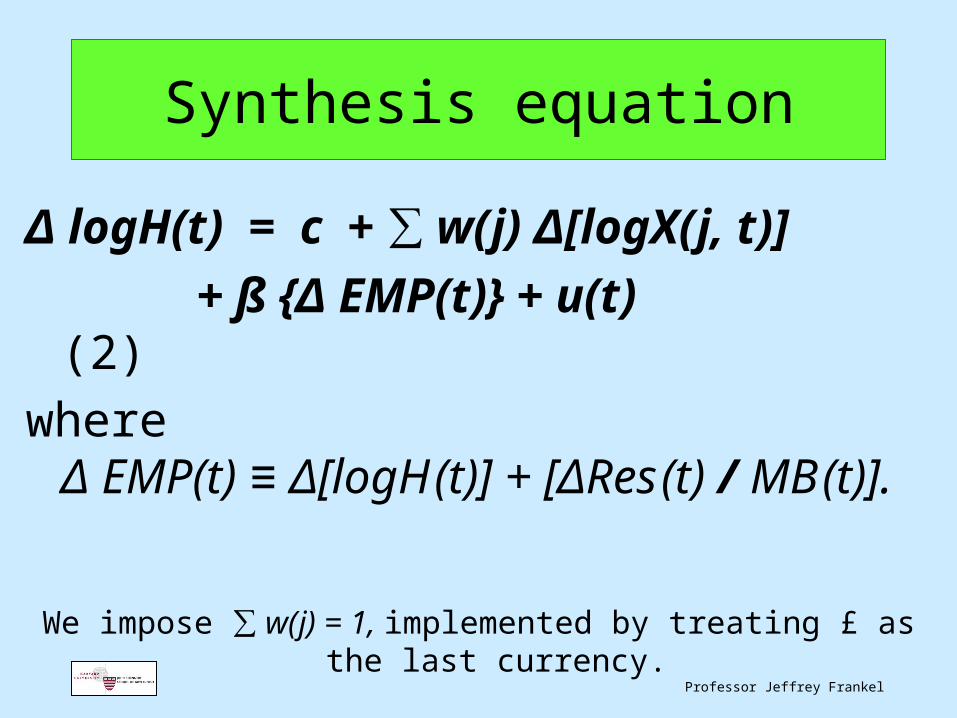
Synthesis equation

Δ logH(t) = c + ∑ w(j) Δ[logX(j, t)]

+ ß {Δ EMP(t)} + u(t) (2)

where Δ EMP(t) ≡ Δ[logH (t)] + [ΔRes (t) / MB (t)].

We impose ∑ w(j) = 1, implemented by treating £ as the last currency.

Appendix 4

More oninflation targetsthat emphasize

export product prices

PPT

PEP

Professor Jeffrey Frankel

Recap of Product Price Targeting:

Target an index of domestic production prices. [1]

The important point:include export commodities in the index and exclude import commodities, whereas the CPI does it the other way around.

[1] Frankel (2011).

PPT

In practice, most IT proponents agree central banks should not tighten to offset oil price shocks

• They want focus on core CPI, excluding food & energy.

• But – food & energy ≠ all supply shocks.

– Use of core CPI sacrifices some credibility:• If core CPI is the explicit goal ex ante, the public feels confused.• If it is an excuse for missing targets ex post, the public feels tricked.

– The threat to credibility is especially strong where there are historical grounds for believing that government officials fiddle with the CPI for political purposes.

– Perhaps for that reason, IT central banks apparently do respond to oil shocks by tightening/appreciating….

Professor Jeffrey Frankel

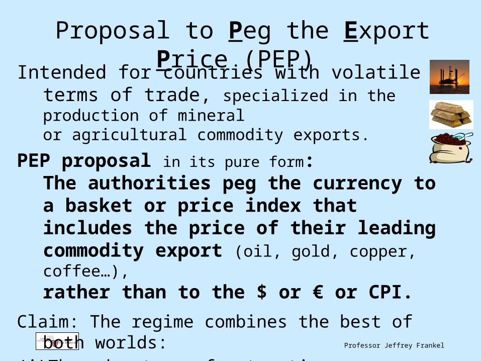
Proposal to Peg the Export Price (PEP)

Intended for countries with volatile terms of trade, specialized in the production of mineral or agricultural commodity exports.

PEP proposal in its pure form: The authorities peg the currency to a basket or price index that includes the price of their leading commodity export (oil, gold, copper, coffee…),

rather than to the $ or € or CPI.

Claim: The regime combines the best of both worlds:

(i) The advantage of automatic accommodation to terms of trade shocks, together with

(ii) the advantages of a nominal anchor and integration.

Professor Jeffrey Frankel

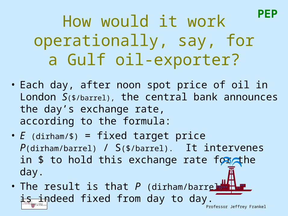
How would it work operationally, say, for a Gulf oil-exporter?

• Each day, after noon spot price of oil in London S($/barrel), the central bank announces the day’s exchange rate, according to the formula:

• E (dirham/$) = fixed target price P(dirham/barrel) / S($/barrel). It intervenes in $ to hold this exchange rate for the day.

• The result is that P (dirham/barrel) is indeed fixed from day to day.

PEP

Professor Jeffrey Frankel

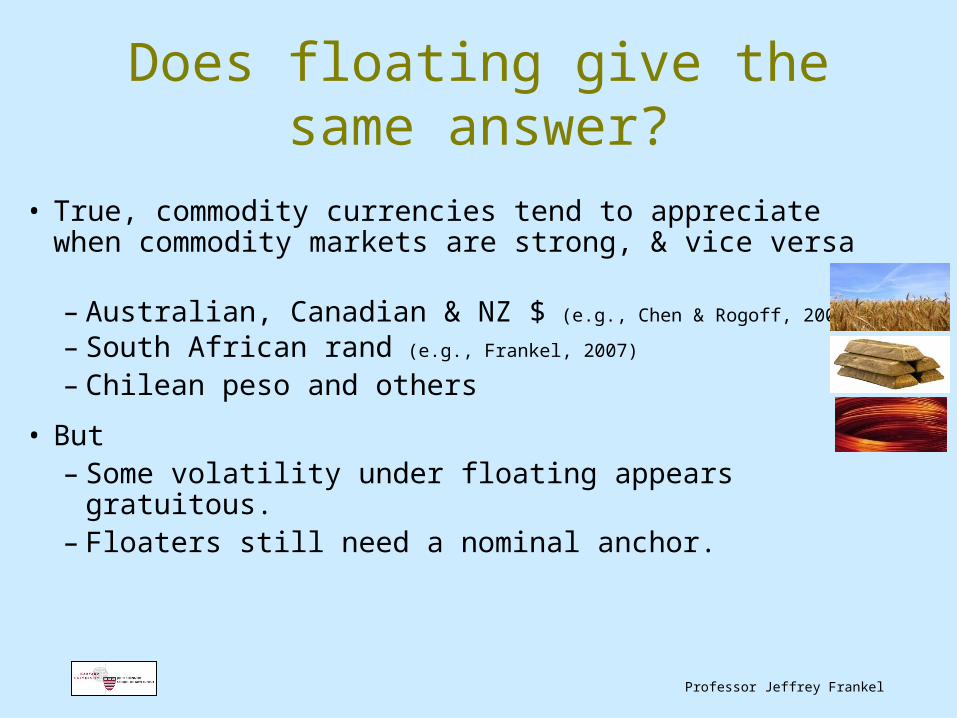
Does floating give the same answer?

• True, commodity currencies tend to appreciate when commodity markets are strong, & vice versa

– Australian, Canadian & NZ $ (e.g., Chen & Rogoff, 2003)

– South African rand (e.g., Frankel, 2007)

– Chilean peso and others

• But– Some volatility under floating appears gratuitous.– Floaters still need a nominal anchor.

Professor Jeffrey Frankel

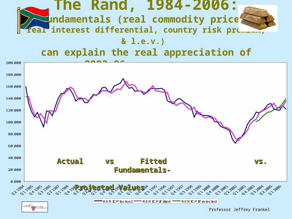
The Rand, 1984-2006:Fundamentals (real commodity prices,

real interest differential, country risk premium, & l.e.v.) can explain the real appreciation of 2003-06 – Frankel (SAJE, 2007).

0.000

20.000

40.000

60.000

80.000

100.000

120.000

140.000

160.000

180.000

200.000

RERICPIactual RERICPIFitted RERICPIProjected

Actual vs Fitted vs. Actual vs Fitted vs. Fundamentals-Fundamentals-

Projected Projected ValuesValues

Professor Jeffrey Frankel

PEP, in its strict form, has some disadvantages

• Passes every fluctuation in world commodity prices straight through to domestic-currency prices of other TGs, creating high volatility

– Even for countries where non-commodity TGs are a small share of the economy, some would like to nurture this sector,

• so as to encourage diversification in the long run.• Exposing it to full volatility could shrink non-commodity TG sector.

– The volatility is undesirable, in particular, for those short-term fluctuations that are likely to be reversed.

– Better to dampen real exchange rate fluctuations a bit, until terms of trade shift appears permanent.

PEP

In practice, most IT proponents agree central banks should not tighten to offset oil price shocks

• They want focus on core CPI, excluding food & energy.

• But – food & energy ≠ all supply shocks.

– Use of core CPI sacrifices some credibility:• If core CPI is the explicit goal ex ante, the public feels confused.• If it is an excuse for missing targets ex post, the public feels tricked.

– The threat to credibility is especially strong where there are historical grounds for believing that government officials fiddle with the CPI for political purposes.

– Perhaps for that reason, IT central banks apparently do respond to oil shocks by tightening/appreciating….

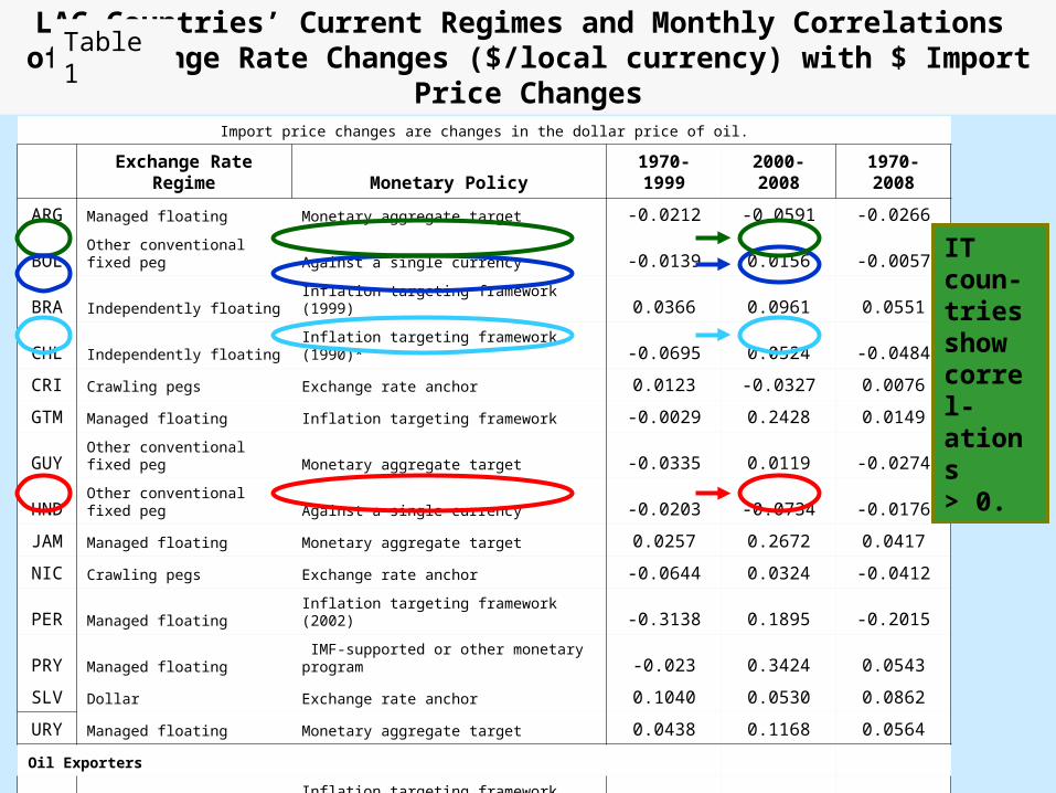
Table 1: LACA Countries’ Current Regimes and Monthly Correlations of Exchange Rate Changes ($/local currency) with Dollar Import Price Changes

Import price changes are changes in the dollar price of oil.

  Exchange Rate Regime Monetary Policy 1970-1999 2000-2008 1970-2008

ARG Managed floating Monetary aggregate target -0.0212 -0.0591 -0.0266

BOL Other conventional fixed peg Against a single currency -0.0139 0.0156 -0.0057

BRA Independently floating Inflation targeting framework (1999) 0.0366 0.0961 0.0551

CHL Independently floating Inflation targeting framework (1990)* -0.0695 0.0524 -0.0484

CRI Crawling pegs Exchange rate anchor 0.0123 -0.0327 0.0076

GTM Managed floating Inflation targeting framework -0.0029 0.2428 0.0149

GUY Other conventional fixed peg Monetary aggregate target -0.0335 0.0119 -0.0274

HND Other conventional fixed peg Against a single currency -0.0203 -0.0734 -0.0176

JAM Managed floating Monetary aggregate target 0.0257 0.2672 0.0417

NIC Crawling pegs Exchange rate anchor -0.0644 0.0324 -0.0412

PER Managed floating Inflation targeting framework (2002) -0.3138 0.1895 -0.2015

PRY Managed floating IMF-supported or other monetary program -0.023 0.3424 0.0543

SLV Dollar Exchange rate anchor 0.1040 0.0530 0.0862

URY Managed floating Monetary aggregate target 0.0438 0.1168 0.0564

Oil Exporters        

COL Managed floating Inflation targeting framework (1999) -0.0297 0.0489 0.0046

MEX Independently floating Inflation targeting framework (1995) 0.1070 0.1619 0.1086

TTO Other conventional fixed peg Against a single currency 0.0698 0.2025 0.0698

VEN Other conventional fixed peg Against a single currency -0.0521 0.0064 -0.0382

* Chile declared an inflation target as early as 1990; but it also had an exchange rate target, under an explicit band-basket-crawl regime, until 1999. 

LAC Countries’ Current Regimes and Monthly Correlations of Exchange Rate Changes ($/local currency) with $ Import Price Changes

Table 1

ITcoun-triesshowcorrel-ations> 0.

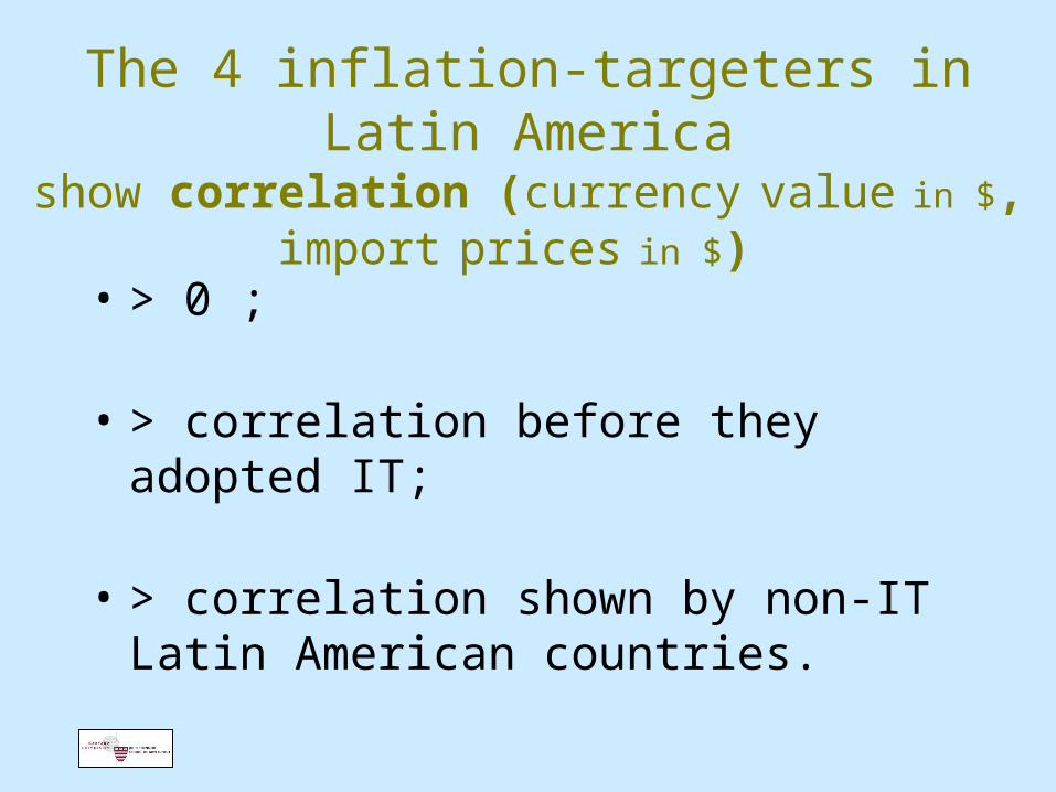
The 4 inflation-targeters in Latin Americashow correlation (currency value in $, import prices in $)

• > 0 ;

• > correlation before they adopted IT;

• > correlation shown by non-IT Latin American countries.

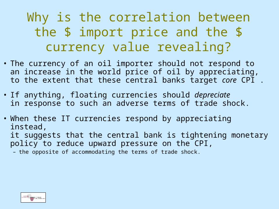
Why is the correlation between the $ import price and the $ currency value revealing?

• The currency of an oil importer should not respond to an increase in the world price of oil by appreciating, to the extent that these central banks target core CPI .

• If anything, floating currencies should depreciate in response to such an adverse terms of trade shock.

• When these IT currencies respond by appreciating instead, it suggests that the central bank is tightening monetary policy to reduce upward pressure on the CPI, – the opposite of accommodating the terms of trade shock.

Professor Jeffrey Frankel

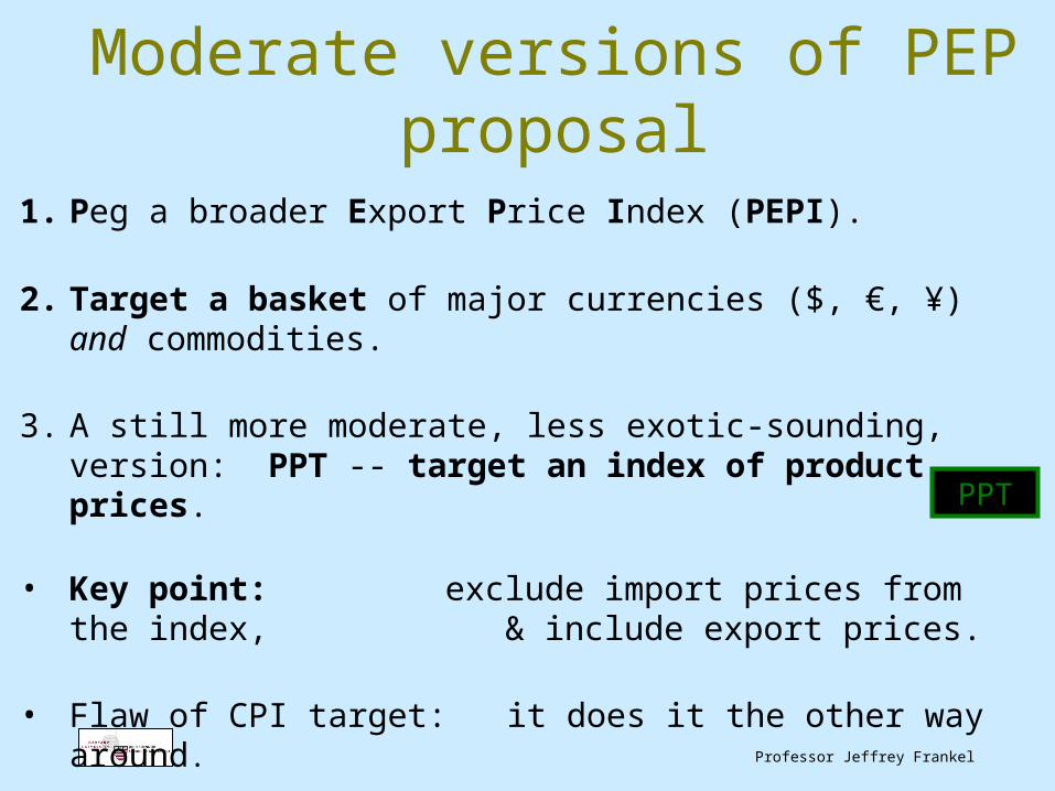
Moderate versions of PEP proposal

1. Peg a broader Export Price Index (PEPI).

2. Target a basket of major currencies ($, €, ¥) and commodities.

3. A still more moderate, less exotic-sounding, version: PPT -- target an index of product prices.

• Key point: exclude import prices from the index, & include export prices.

• Flaw of CPI target: it does it the other way around.

PPT

Professor Jeffrey Frankel

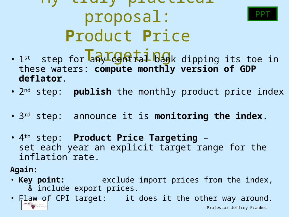
My truly practical proposal:Product Price Targeting

• 1st step for any central bank dipping its toe in these waters: compute monthly version of GDP deflator.

• 2nd step: publish the monthly product price index

• 3rd step: announce it is monitoring the index.

• 4th step: Product Price Targeting – set each year an explicit target range for the inflation rate.

Again:• Key point: exclude import prices from the index,

& include export prices. • Flaw of CPI target: it does it the other way around.

PPT