NBER WORKING PAPER SERIES

ESTIMATION OF DE FACTO FLEXIBILITY PARAMETER AND BASKET WEIGHTSIN EVOLVING EXCHANGE RATE REGIMES

Jeffrey A. FrankelDaniel Xie

Working Paper 15620http://www.nber.org/papers/w15620

NATIONAL BUREAU OF ECONOMIC RESEARCH1050 Massachusetts Avenue

Cambridge, MA 02138December 2009

The authors would like to thank Agnès Bénassy-Quéré, Oyebola Olabisi, Carmen Reinhart and Shang-JinWei for comments. A shorter version of this paper is expected to appear in AER Papers and Proceedings,May 2010, and will eliminate most of Sections III and IV and the Tables, to meet space constraints. The views expressed herein are those of the authors and do not necessarily reflect the views of theNational Bureau of Economic Research.

NBER working papers are circulated for discussion and comment purposes. They have not been peer-reviewed or been subject to the review by the NBER Board of Directors that accompanies officialNBER publications.

© 2009 by Jeffrey A. Frankel and Daniel Xie. All rights reserved. Short sections of text, not to exceedtwo paragraphs, may be quoted without explicit permission provided that full credit, including © notice,is given to the source.

Estimation of De Facto Flexibility Parameter and Basket Weights in Evolving Exchange RateRegimesJeffrey A. Frankel and Daniel XieNBER Working Paper No. 15620December 2009JEL No. F31,F41

ABSTRACT

A new technique for estimating countries’ de facto exchange rate regimes synthesizes two approaches.One approach estimates the implicit de facto basket weights in an OLS regression of the local currencyvalue rate against major currency values. Here the hypothesis is a basket peg with little flexibility.The second estimates the de facto degree of exchange rate flexibility by observing how exchangemarket pressure is allowed to show up. Here the hypothesis is an anchor to the dollar or some othersingle major currency, but with a possibly substantial degree of exchange rate flexibility around thatanchor. It is important to have available a technique that can cover both dimensions: inferring anchorweights and the flexibility parameter. We test the synthesis technique on a variety of fixers, floaters,and basket peggers. We find that real world data demand a statistical technique that allows parametersand regimes to shift frequently. Accordingly we here take the next step in estimation of de facto exchangerate regimes: endogenous estimation of parameter breakpoints, following Bai and Perron.

Jeffrey A. FrankelKennedy School of GovernmentHarvard University79 JFK StreetCambridge, MA 02138and NBERjeffrey_frankel@harvard.edu

Daniel XiePeterson Institute for International Economics1750 Massachusetts Avenue, NWWashington, DC 20036dxie@piie.com

2

As is by now well-known, the exchange rate regimes that countries follow in

practice (de facto) often depart from the regimes that they announce officially (de jure).

Many countries that say they float in fact intervene heavily in the foreign exchange

market.1 Many countries that say they fix in fact devalue when trouble arises.2 Many

countries that say they target a basket of major currencies in fact fiddle with the weights.3

A number of economists have offered attempts at de facto classifications, placing

countries into the “true” categories, such as fixed, floating, and intermediate.4

Unfortunately, these classification schemes disagree with each other as much as they

disagree with the de jure classification.5 Something must be wrong.

I. The existing techniques for estimating de facto regimes and their drawbacks

Several things are wrong. First, attempts to infer statistically a country’s degree

of exchange rate flexibility from the variability of its exchange rate alone ignore that

some countries experience greater shocks than others.

1 “Fear of floating:” Calvo and Reinhart (2001, 2002); Reinhart (2000). 2 “The mirage of fixed exchange rates:” Obstfeld and Rogoff (1995). Klein and Marion

(1997). 3 Frankel, Schmukler and Servén (2000).

4 Important examples include Ghosh, Gulde and Wolf (2000), Reinhart and Rogoff

(2004), Shambaugh (2004), and those cited in other footnotes. Tavlas, Dellas and

Stockman (2008) survey the literature.

5 Frankel (Table 1, 2004) and Bénassy-Quéré, et al (Table 5, 2004).

3

I.1 Exchange Market Pressure

That problem can be addressed by comparing exchange rate variability to foreign

exchange reserve variability, as do Calvo and Reinhart (2002) and Levy-Yeyati and

Sturzenegger (2003, 2005). A useful way to specify this approach is in terms of

Exchange Market Pressure, defined as the sum of the change in the value of a currency

and the change in its reserves.6 Exchange Market Pressure represents shocks in

demand for the currency. The flexibility parameter can be estimated from the propensity

of the central bank to let these shocks show up in the price of the currency (floating) or

the quantity of the currency (fixed) or somewhere in between (intermediate exchange rate

regime). But even these papers have a second limitation: they generally impose the

choice of the major currency around which the country in question defines its value, most

often the dollar. For some countries -- to whatever extent the authorities seek to stabilize

the exchange rate -- it is fairly evident what the anchor currency must be (the dollar for

countries in the Caribbean and most of Latin America, the euro in most of Central

Europe). But for others it is much less evident, especially those with geographically

diversified trade (Asia, the Pacific, the Middle East, much of Africa, and the Southern

Cone of South America). In many cases, one cannot even presume that the anchor is a

6 The progenitor of the Exchange Market Pressure variable, in a rather different context, was

Girton and Roper (1977). Here we impose the a priori constraint that a one percentage increase in

the foreign exchange value of the currency and a one percentage increase in the supply of the

currency (the change in reserves as a share of the monetary base) have equal weights, rather than

normalizing by standard deviations as Girton and Roper did.

4

single major currency. It would be better to estimate endogenously whether the anchor

currency is the dollar, the euro, some other currency, or some basket of currencies.

I.2 Basket Weights

A third set of papers is designed precisely to do this, to estimate the anchor

currency, or more generally to estimate the currencies in the basket and their respective

weights.7 The approach is simply to run a regression of the change in the value of the

local currency against the changes in the values of the dollar, euro, and other major

currencies that are potential candidates for the anchor currency or basket of currencies.

In the special case where the country in question in fact does follow a perfect basket peg,

the technique is an exceptionally apt application of OLS regression. Under the null

hypothesis, it should be easy to recover precise estimates of the weights. The fit should

be perfect, an extreme rarity in econometrics: the standard error of the regression should

be zero, and R2 = 100%.

The reason to work in terms of changes rather than levels is the likelihood of non-

stationarity. Concern for nonstationarity in this equation goes beyond the common

refrain of modern time series econometrics, the inability to reject statistically a unit root.

There is often good reason a priori to consider the possibility that the regime builds in a

trend. In the context of countries with a history of high inflation, the hypothesis of

interest is that the currency regime is a crawling peg, that is, that there is a steady

7 Examples include Frankel (1993), Frankel and Wei (1994, 1995, 2007), Bénassy-Quéré

(1999), and Bénassy-Quéré, Coeuré, and Mignon (2004), among others.

5

negative trend in its value.8 In the context of the Chinese yuan in the years since 1994,

the hypothesis of interest is a positive trend in its value.9 Working in terms of first

differences is a clean way to allow for nonstationarity. One simply includes a constant

term to allow for the possibility of a crawl in the currency, whether against the dollar

alone or a broader basket.

Although the equation is very well-specified under the null hypothesis of a basket

peg or other peg, it is on less firm ground under the alternative hypothesis. The

approach neglects to include anything to help make sense out of the error term under the

alternative hypothesis that the country is not perfectly pegged to a major currency or to a

basket, but rather has adopted a degree of flexibility around its anchor. In other words,

the limitation of the implicit-weights estimation approach is the same as the virtue of the

flexibility-parameter estimation approach and vice versa. The latter is well-specified to

8 The hypothesis of a constant rate of crawl is readily combined with the hypothesis that

the anchor is a basket, and even with the hypothesis of variability around the anchor. The

combined BBC regime (Basket / Band / Crawl) has been recommended for a variety of

countries (Williamson, 2001). It was, for example, the regime followed by Chile in the

1990s, de facto as well as de jure (Frankel, Schmukler and Servén, 2000).

9 In 2005, Chinese authorities announced a switch to a new exchange rate regime: The

exchange rate would henceforth be set with reference to a basket of other currencies, with

numerical weights unannounced, allowing cumulatively a movement of up to +/- .3% per

day. Initial applications of the implicit basket estimation technique to the yuan exchange

rate suggested that the de facto regime continued to be essentially a dollar peg in 2005

and 2006. E.g., Ogawa (2006), Frankel and Wei (2007) and other papers cited there.

6

estimate the flexibility parameter only if the anchor is already known, while the former is

well-specified to estimate the anchor only if there is no flexibility.

Frankel and Wei (2008) synthesize the technique that estimates the flexibility

parameter with the technique that estimates the degree of flexibility. The synthesis

technique brings the two branches of the literature together to produce a complete

equation suitable for use in inferring the de facto regime across the spectrum of flexibility

and across the array of possible anchors.10

I.3 Regime change

All these approaches, including the synthesis technique, suffer from a further

limitation. In practice many currencies, perhaps the majority, do not maintain a single

consistent regime for more than a few years at a time, but rather switch parameters every

few years and even switch regimes.11 The official regime of Chile, for example,

changed parameters – basket weights, width of band, rate of crawl -- 18 times from

September 1982 to September 1999 (after which it started floating), an average of once a

year. If such changes always fell on January 1, one might have some hope of being able

to estimate the equation year by year, though this would be difficult if one were limited to

10 Frankel (2009) applies the synthesis technique to data on the Chinese exchange rate

from 2005 to 2008, finding that the yuan during the latter part of this period did move

away from the dollar peg, shifting some weight to the euro.

11 Masson (2001).

7

only 12 monthly observations. Since the parameter changes can come anytime, the

standard strategy, of estimating an equation for each year, or each interval of two years,

or more years, cannot hope to capture the reality. The frequent changes in regimes and

parameters that many countries experience may be the most important reason why

different authors’ classification schemes give different results among the universe of

currencies, and none seems to get fully at the truth.

The next step is to apply statistical techniques that allow for the possibility that

the regime and parameter governing a currency shifts, and shifts at irregular intervals. If

one knows the hypothesized date of a shift, e.g., because it is officially announced, then

one can test that the structural break took place de facto by means of the classic test of

Chow (1960). More often, however, the structural breaks could fall at any date. In this

paper we adopt the estimation technology developed by Bai and Perron (1998, 2003),

who provided estimators, test statistics, and efficient algorithms appropriate to a linear

model with multiple possible structural changes at unknown dates.

II. The synthesis equation

Algebraically, if the home currency, with value defined as H, is pegged to

currencies with values defined as X1, X2, … and Xn, and weights equal to w1, w2, … and

wn, then

logH(t+s) - logH(t) = c + ∑ w(j) [logX(j, t+s) - logX(j, t)] (1)

8

One methodological question must be addressed. How do we define the “value”

of each of the currencies? This is the question of the numeraire. 12 If the exchange rate is

truly a basket peg, the choice of numeraire currency is immaterial; we estimate the

weights accurately regardless.13 If the true regime is more variable than a rigid basket

peg, then the choice of numeraire does make some difference to the estimation. Some

authors in the past have used a remote currency, such as the Swiss franc.

A weighted index such as a trade-weighted measure or the SDR (Special Drawing

Right, an IMF unit composed of a basket of most important major currencies) is probably

more appropriate. Here is why. Assume the true regime is a target zone or a managed

float centered around a reference basket, where the authorities intervene to an extent that

depends on the magnitude of the deviation; this seems the logical alternative hypothesis

in which a strict basket peg is nested. The error term in the equation represents shocks in

demand for the currency that the authorities allow to be partially reflected in the

exchange rate (but only partially, because they intervene if the shocks are large). Then

12 Frankel and Wei (1995) used the SDR as numeraire; Frankel (1993) used purchasing power

over a consumer basket of domestic goods; Frankel and Wei (1994, 2006) and Ohno (1999) used

the Swiss franc; Bénassy-Quéré (1999), the dollar; Frankel, Schmukler and Servén (2000), a

GDP-weighted basket of five major currencies. Bénassy-Quéré, Coeuré, and Mignon (2004)

propose a modification of the methodology, with a method of moments approach; the advantage

of the modification is that it does not depend on the choice of a numeraire currency.

13 If the linear equation holds precisely in terms of any one “correct” numeraire, then add the log

exchange rate between that numeraire and any arbitrary unit to see that the equation also holds

precisely in terms of the arbitrary numeraire. This assumes the weights add to 1, and there is no

error term, constant term, or other non-currency variable.

9

one should use a numeraire that is similar to the yardstick used by the authorities in

measuring what constitutes a large deviation. The authorities are unlikely to use the

Swiss franc or Canadian dollar in thinking about the size of deviations from their

reference point. They are more likely to use a weighted average of major currencies. If

we use a similar measure in the equation, it should help minimize the possibility of

correlation between the error term and the numeraire. Similarly, if there is a trend in the

exchange rate equation (a constant term in the changes equation) representing deliberate

gradual appreciation of the currency, then the value of the local currency should be

defined in terms of whatever weighted exchange rate index the authorities are likely to

use in thinking about the trend. These considerations suggest a numeraire that is itself

composed of a basket of currencies. Here, as in Frankel and Wei (1995, 2007), we

choose the SDR.14

There is a good argument for constraining the weights on the currencies to add up

to 1. The easiest way to implement the adding up constraint is to run the regressions with

the changes in the log of the local currency value on the left-hand side of the equation

transformed by subtracting off the changes in the log value of one of the currencies, say

the pound, and the changes in the values of the other major currencies on the right-hand

side transformed in the same way. To see this, we repeat equation (1):

Δ log Ht = c + ∑ w(j) [Δ logX(j)t ]

= c + β(1) Δ log $ t + β(2) Δ log ¥t + β(3) Δ log €t + α Δ log £t

We want to impose the adding up constraint α = 1 - β(1) - β(2) - β(3) …

14 Among the extensions and robustness checks in Frankel and Wei (2007) was a check whether

the results were sensitive to the numeraire, as between the SDR and gold.

10

We implement it by running the regression equation (2):

[Δ logH t - Δ log £t ] = c + β(1) [Δ log $t - Δ log £t ]

+ β(2)[ Δ log ¥t - Δ log £t] + β(3) [Δ log €t -Δ log £t] (2)

One can recover the implicit weight on the value of the pound by adding the

estimated weights on the non-dollar currencies, and subtracting the sum from 1. (We

usually report this residual coefficient estimate in the last row of the tables.) Imposing

the constraint sharpens the estimates a bit.15

Our synthesis equation is:

Δ log H t = c + ∑ w(j) Δ logX(j) t + δ { Δ EMP t } + u t (3)

where Δ emp t denotes the percentage change in exchange market pressure, that is, the

increase in international demand for the Home currency, which may show up either in the

its price or its quantity, depending on the policies of the monetary authorities. Here we

define the percentage change in total exchange market pressure by

Δ EMP t ≡ Δ logH t + ΔRes t /MB t ,

where Res ≡ foreign exchange reserves and MB ≡ Monetary Base. The w(j) coefficients

capture the de facto weights on the constituent currencies. The coefficient δ captures the

de facto degree of exchange rate flexibility. A high δ means the currency floats purely,

because there is little foreign exchange market intervention (few changes in reserves; in

15 The choice of which currency to drop from the right-hand side in order to impose the adding up

constraint, in this case the pound, is completely immaterial to the estimates. The choice of which

currency to use as numeraire, by contrast, can make a difference to the estimates (to the extent

that the true regime differs substantially from a perfect basket peg).

11

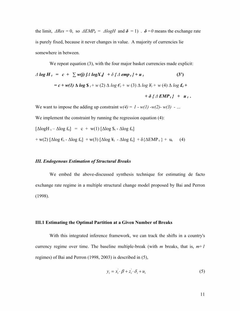
the limit, ΔRes = 0, so ΔEMPt = ΔlogH and δ = 1) . δ =0 means the exchange rate

is purely fixed, because it never changes in value. A majority of currencies lie

somewhere in between.

We repeat equation (3), with the four major basket currencies made explicit:

Δ log H t = c + ∑ w(j) [Δ logX t] + δ { Δ emp t } + u t (3’)

= c + w(1) Δ log $ t + w (2) Δ log €t + w (3) Δ log ¥t + w (4) Δ log £t +

+ δ { Δ EMP t } + u t .

We want to impose the adding up constraint w(4) = 1 - w(1) -w(2)- w(3) - …

We implement the constraint by running the regression equation (4):

[ΔlogH t – Δlog £t] = c + w(1) [Δlog $t - Δlog £t]

+ w(2) [Δlog €t - Δlog £t] + w(3) [Δlog ¥t - Δlog £t] + δ{ΔEMP t } + ut (4)

III. Endogenous Estimation of Structural Breaks

We embed the above-discussed synthesis technique for estimating de facto

exchange rate regime in a multiple structural change model proposed by Bai and Perron

(1998).

III.1 Estimating the Optimal Partition at a Given Number of Breaks

With this integrated inference framework, we can track the shifts in a country's

currency regime over time. The baseline multiple-break (with m breaks, that is, m+1

regimes) of Bai and Perron (1998, 2003) is described in (5),

tittt uzxy +⋅+⋅= δβ '' (5)

12

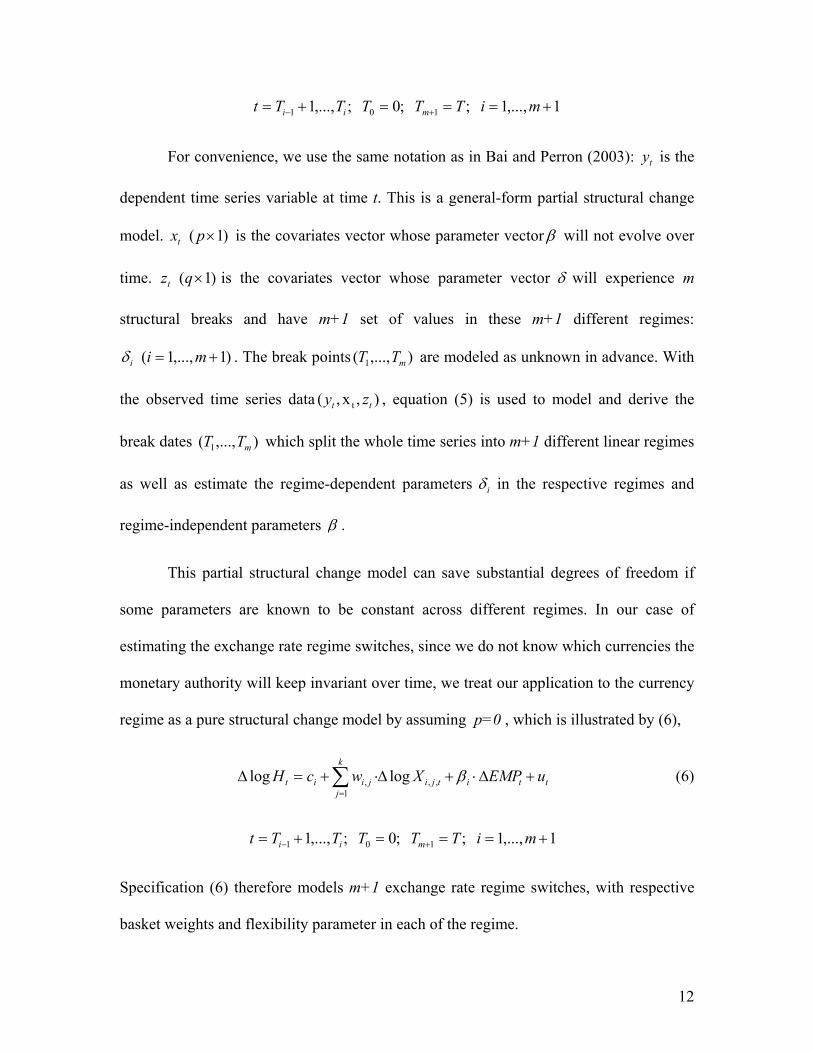
1,...,1 ; ;0 ;,...,1 101 +===+= +− miTTTTTt mii

For convenience, we use the same notation as in Bai and Perron (2003): ty is the

dependent time series variable at time t. This is a general-form partial structural change

model. )1( ×pxt is the covariates vector whose parameter vectorβ will not evolve over

time. )1( ×qzt is the covariates vector whose parameter vector δ will experience m

structural breaks and have m+1 set of values in these m+1 different regimes:

)1,...,1( += miiδ . The break points ),...,( 1 mTT are modeled as unknown in advance. With

the observed time series data ),x,( t tt zy , equation (5) is used to model and derive the

break dates ),...,( 1 mTT which split the whole time series into m+1 different linear regimes

as well as estimate the regime-dependent parameters iδ in the respective regimes and

regime-independent parameters β .

This partial structural change model can save substantial degrees of freedom if

some parameters are known to be constant across different regimes. In our case of

estimating the exchange rate regime switches, since we do not know which currencies the

monetary authority will keep invariant over time, we treat our application to the currency

regime as a pure structural change model by assuming p=0 , which is illustrated by (6),

ttitji

k

jjiit uEMPXwcH +Δ⋅+Δ⋅+=Δ ∑

=

β,,1

, loglog (6)

1,...,1 ; ;0 ;,...,1 101 +===+= +− miTTTTTt mii

Specification (6) therefore models m+1 exchange rate regime switches, with respective

basket weights and flexibility parameter in each of the regime.

13

Bai and Perron (1998) adopt the general least-squares principle to estimate the

break dates: for any of the m-partitions ),...,( 1 mTT , a set of parameters ic , jiw , and iβ are

derived to minimize the sum of squared residuals as represented by (7),

2

1,,

1,

1

1 1

loglog∑ ∑∑+= =

+

= −

⎥⎦

⎤⎢⎣

⎡Δ⋅−Δ−−Δ

i

i

T

Tttitji

k

jjiit

m

iEMPXwcH β (7)

ic , jiw , and iβ are the estimated set of parameters for each possible m-

partition ),...,( 1 mTT , that is, ),...,( 1 mii TTcc = , ),...,( 1 mii TTββ = and ),...,( 1,, mjiji TTww = .

Corresponding to the specific set of parameters ic , jiw , and iβ for a m-partition ),...,( 1 mTT ,

a minimized sum of squared residuals is calculated, i.e. by substituting the values

of ic , jiw , and iβ into (7), the objective function.

The last step is to search for the best m-partition ),...,( 1 mTT that can minimize the

partition-dependent objective function globally as shown by (8),

2

1,,

1,

1

1,...,

^

1

^

11

loglog),...,( minarg ∑ ∑∑+= =

+

= −

⎥⎦

⎤⎢⎣

⎡Δ⋅−Δ⋅−−Δ=

i

im

T

Tttitji

k

jjiit

m

iTT

m EMPXwcHTT β (8)

Finally, according to the estimated best m-partition ),...,(^

1

^

mTT , we can easily

recover the relevant set of coefficients ),...,(^

1

^^^

mii TTcc = , ),...,(^

1

^

,

^

,

^

mjiji TTww = and

),...,(^

1

^^^

mii TTββ = , which correspond to the parameters for each of the respective

regimes.

A grid search algorithm can be used to seek for the global minimizer. However,

the computational complexity of the traditional grid search algorithm to estimate a global

14

minimizer like (8) is at the order of )( mTO operations, which is formidable even when m

just grows moderately larger than 2. The additional innovation of Bai and Perron (2003)

is to apply a dynamic programming principle to this global minimization procedure,16

which finally limits the cost of computation to )( 2TO . We follow their computational

approach in this paper.

III.2 Testing and Estimating the Number of Breaks

The methodology discussed in Section 3.1 can help us to locate the best m-

partition and find out the associated regime-specific basket weights and flexibility

parameter, assuming we have known the explicit number of breaks m. However, we do

not know the accurate break number in advance. Then we also need a reliable way to

estimate the break number m.

Bai and Perron (1998) proposed a sequential test supF(ℓ+1/ℓ), i.e. testing ℓ versus

ℓ+1 breaks. This testing approach is also based on the general least-squares principle: if

the value of the objective function (the minimized least-squares) by assuming ℓ+1 breaks

is significantly smaller than the case by assuming ℓ breaks, the hypothesis of ℓ breaks

will be rejected in favor of a ℓ+1 breaks alternative. The recommended procedure by Bai

and Perron (2003) is to firstly test 0 versus 1 break; if we can reject the hypothesis of zero

break, then go on to test 1 versus 2 break; in other words, we sequentially apply the test

of supF(ℓ+1/ℓ), until the hypothesis of m+1 breaks is rejected versus the alternative of

m breaks. Then we can make the conclusion that an m-break-partition model is

16 Detailed discussion on dynamic programming is available in Cormen, et al (2001).

15

appropriate and derive the corresponding estimates of parameters in each of the m+1

regimes in terms of the methodology of Section 3.1.

IV. An Illustration: Estimation for Five Currencies

Exchange rate data are available on a daily basis, but data on foreign exchange

reserves and the monetary base have historically been available only on a monthly basis

for most developing countries. If structural shifts occur as frequently as once a year, we

will have a hard time discerning this with the monthly data, no matter what the

econometric technique. We limit the anchor currency or basket to four major candidates

– dollar, euro, yen and pound -- but this still requires estimation of five parameters: three

currency weights, the flexibility parameter, and the crawl term.

Fortunately, some of the emerging market currencies of greatest interest now

make available their data on reserves on a weekly basis or even daily in the case of a few

Latin American countries. We conclude this paper by illustrating the estimation

technique for five of these currencies, in Table 1.

For all five currencies, the statistical estimates suggest managed floats during

most of the period 1999-2009. This was a new development for emerging markets.

Most of the countries had some variety of a peg before the currency crises of the 1990s.

But the Bai-Perron test shows statistically significant structural breaks for every currency,

even when the threshold is set high, at the 1% level of statistical significance.

Table 1A reports estimation for the Mexican peso using weekly data (5 structural

breaks). The peso is known as a floater. To the extent that Mexico intervenes to reduce

16

exchange rate variation, the dollar is the primary anchor, but there also appears to have

been some weight on the euro starting in 2003. From August 2006 to December 2008,

the coefficient on Exchange Market Pressure is essentially zero, surprisingly, suggesting

heavier intervention around a dollar target. But in the period starting December 2008, the

peso once again moved away from the currency to the north, when the worst phase of the

global liquidity crisis hit and the dollar appreciated.

For the other four currencies, although the exchange rate and reserve data are both

available weekly, the monetary base is not. Recall that our way of scaling the change in

reserves it so express it as a share of the monetary base. For this purpose, we interpolate

between the monthly monetary base data.

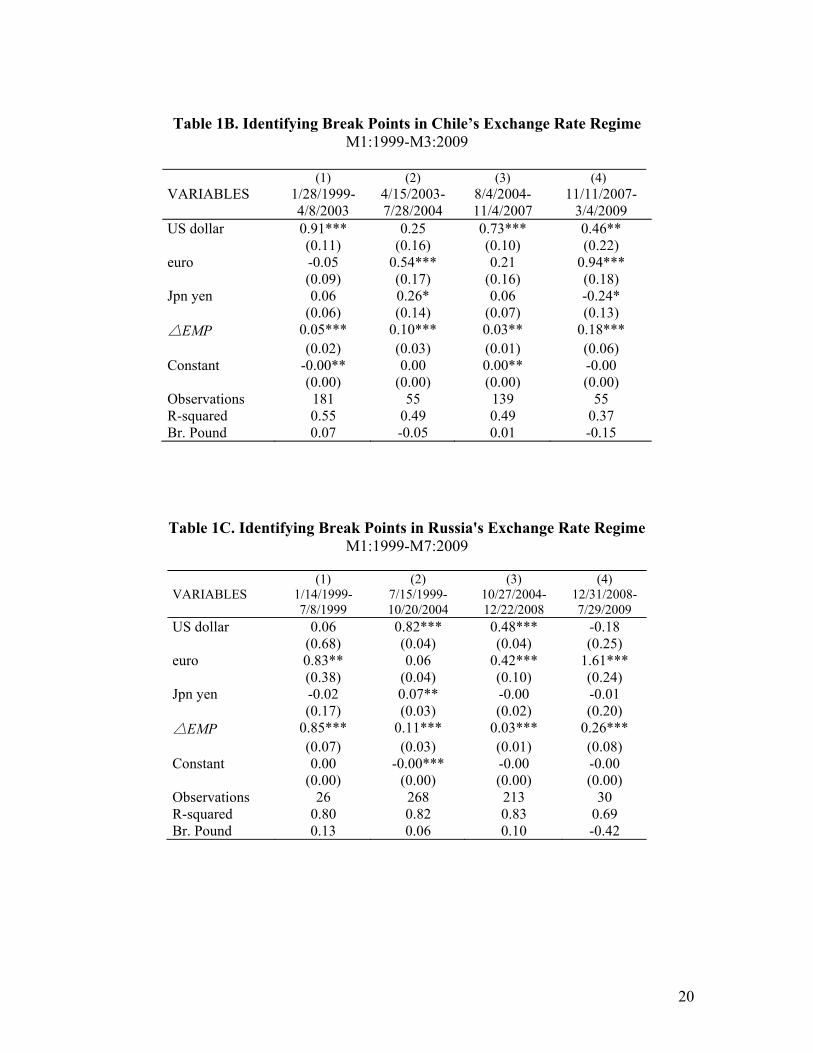
Chile (with 3 estimated structural breaks) appears a managed floater throughout.

The anchor is exclusively the dollar in some periods, but puts significant weight on the

euro in other periods. Russia (3 structural breaks) is similar, except that the weight on

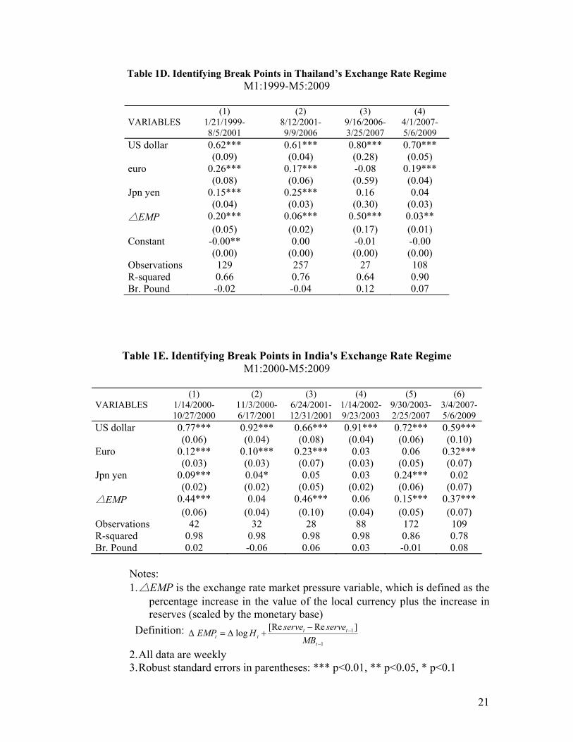
the dollar is always significantly less than 1. For Thailand (3 structural breaks), the share

of the dollar in the anchor basket is slightly above .6, but usually significantly less than 1.

The euro and yen show weights of about .2 each between January 1999 and September

2006. India (5 structural breaks) apparently fixed its exchange rate during two of the

sub-periods, but pursued a managed float in the other four sub-periods. The dollar was

always the most important of the anchor currencies, but the euro was also significant in

four out of six sub-periods, and the yen in two.

The estimation results are no tidier than the reality of these currencies, which do

not stick with any one clean regime for long. Applications of the technique to examples

of currencies following clean pegs to a basket or to a single currency are available

17

elsewhere.17 Possible future extensions include providing a classification scheme that

includes most or all members of the IMF, attempting to analyze reasons for parameter

shifts, and applying a Threshold Autoregressive Technique to capture more accurately the

right specification for those countries believed to be following a target zone, rather than

more general managed floating.

References

Bai, Jushan, and Pierre Perron. 1998. "Estimating and Testing Linear Models with Multiple Structural Changes," Econometrica, 66(1): 47-78.

Bai, Jushan and Pierre Perron. 2003. "Computation and analysis of multiple structural change models," Journal of Applied Econometrics, 18(1): 1-22.

Bénassy-Quéré, Agnès. 1999. “Exchange Rate Regimes and Policies: An Empirical Analysis.” In Exchange Rate Policies in Emerging Asian Countries. edited by Stefan Collignon, Jean Pisani-Ferry and Yung Chul Park. London: Routledge: 40–64.

Bénassy-Quéré, Agnès, Benoit Coeuré, and Valérie Mignon. 2004. “On the Identification of de facto Currency Pegs,” Journal of the Japanese and International Economies 20(1): 112–27.

Calvo, Guillermo, and Carmen Reinhart. 2001. "Fixing for Your Life." In Brookings Trade Forum 2000, edited by Susan Collins and Dani Rodrik, Washington DC: Brookings Institution.

Calvo, Guillermo, and Carmen Reinhart. 2002. “Fear Of Floating," The Quarterly Journal of Economics, 117(2): 379-408.

Chow, Gregory, 1960, "Tests of Equality Between Sets of Coefficients in Two Linear Regressions. Econometrica, 28(3): 591-605.

Frankel, Jeffrey. 1993. ‘Is Japan Creating a Yen Bloc in East Asia and the Pacific?” In Regionalism and Rivalry: Japan and the US in Pacific Asia, edited by J. Frankel and M. Kahler. Chicago: University of Chicago Press: 53–85.

Frankel, Jeffrey. 2004. “Experience of and Lessons from Exchange Rate Regimes in Emerging Economies,” in Monetary and Financial Integration in East Asia: The Way

17 Frankel and Wei (2008) for some de jure basket peggers (including Latvia, Norway,

Malta , Chile, and the Seychelles). Frankel (2009) for China.

18

Ahead, edited by the Asian Development Bank, 91-138. New York: Palgrave Macmillan Press.

Frankel, Jeffrey. 2009. “New Estimation of China’s Exchange Rate Regime,” Pacific Economic Review 14(3), August (Wiley InterScience, Blackwell Publishing): 346-60. Frankel, Jeffrey, Sergio Schmukler, and Luis Servén. 2000. “Verifiability and the Vanishing Intermediate Exchange Rate Regime.” In Brookings Trade Forum 2000, edited by Susan Collins and Dani Rodrik. Washington, DC: Brookings Institution: 59-123.

Frankel, Jeffrey, and Shang-Jin Wei. 1994. ‘Yen Bloc or Dollar Bloc? Exchange Rate Policies of the East Asian Economies.” In Macroeconomic Linkages edited by Takatoshi. Ito and Anne Krueger, 295–329. Chicago: University of Chicago Press.

Frankel, Jeffrey, and Shang-Jin Wei. 2007. “Assessing China’s Exchange Rate Regime.” Economic Policy 51 (July): 575–614.

Frankel, Jeffrey, and Shang-Jin Wei, 2008, “Estimation of De Facto Exchange Rate Regimes: Synthesis of The Techniques for Inferring Flexibility and Basket Weights.” IMF Staff Papers 55: 384–416.

Ghosh, Atish, Anne-Marie Gulde, and Holger Wolf. 2000. “Currency Boards: More than a Quick Fix?” Economic Policy, 31 (October): 270-335. Girton, Lance and Don Roper. 1977. “A Monetary Model of Exchange Market Pressure Applied to the Postwar Canadian Experience.” American Economic Review 67(4): 537–48.

Klein, Michael, and Nancy Marion. 1997. Explaining the Duration of Exchange-Rate Pegs. Journal of Development Economics 54(2):387-404. Levy-Yeyati, Eduardo, and Federico Sturzenegger. 2003. “To Float or to Trail: Evidence on the Impact of Exchange Rate Regimes on Growth,” American Economic Review 93(4): 1173–93. Levy-Yeyati, Eduardo and Federico Sturzenegger. 2005. “Classifying Exchange Rate Regimes: Deeds vs. Words.” European Economic Review 49(6): 1603–1635.

Masson, Paul. 2001. “Exchange Rate Regime Transitions.” Journal of Development Economics, 64: 571-586. Obstfeld, Maurice, and Kenneth Rogoff. 1995. “The Mirage of Fixed Exchange Rates.” Journal of Economic Perspectives 9(4), Fall:73-96. Ogawa, Eiji. 2006. "The Chinese Yuan after the Chinese Exchange Rate System Reform," China and World Economy, 14(6), Nov.-Dec.: 39-57.

19

Reinhart, Carmen. 2000. “The Mirage of Floating Exchange Rates.” American Economic Review 90 (2): 65-70. Reinhart, Carmen, and Kenneth Rogoff. 2004. “The Modern History of Exchange Rate Arrangements: A Reinterpretation.” Quarterly Journal of Economics, 119(1):1-48.

Shambaugh, Jay. 2004. “The Effect of Fixed Exchange Rates on Monetary Policy.” Quarterly Journal of Economics, 119(1):300-51.

Tavlas, George, Dellas, Harris, and Stockman, Alan, 2008. "The Classification and Performance of Alternative Exchange-Rate Systems," European Economic Review, 52(6): 941-63, August.

Williamson, John. 2001. “The Case for a Basket, Band and Crawl (BBC) Regime for East Asia,” In Future Directions for Monetary Policies in East Asia, edited by David Gruen and John Simon. (Sydney: Reserve Bank of Australia.)

Table 1: Estimation of De Facto Exchange Rate Regimes -- Five Currencies, Weekly Data

Table 1A. Identifying Break Points in Mexican Exchange Rate Regime M1:1999-M7:2009

(1) (2) (3) (4) (5) (6) VARIABLES 1/21/1999-

9/2/2001 9/9/2001-3/18/2003

3/25/2003-7/29/2006

8/5/2006-1/28/2008

2/4/2008- 12/15/2008

12/22/2008-7/29/2009

US dollar 0.92*** 0.88*** 0.62*** 1.11*** 0.96*** 0.20 (0.09) (0.12) (0.07) (0.10) (0.19) (0.22) euro 0.14 -0.09 0.30*** 0.20* 0.51*** 0.51*** (0.08) (0.14) (0.09) (0.11) (0.16) (0.18) Jpn yen -0.05 0.22*** 0.08 -0.34*** -0.33** 0.18 (0.06) (0.07) (0.06) (0.06) (0.12) (0.13) △EMP 0.14*** 0.32*** 0.17*** 0.02 0.07 0.28*** (0.03) (0.03) (0.03) (0.02) (0.07) (0.04) Constant 0.00 -0.00*** -0.00* -0.00 -0.00 0.00 (0.00) (0.00) (0.00) (0.00) (0.00) (0.00) Observations 131 78 168 76 46 29 R-squared 0.62 0.86 0.69 0.67 0.54 0.78 Br. Pound -0.01 -0.01 -0.01 0.02 -0.14 0.11

20

Table 1B. Identifying Break Points in Chile’s Exchange Rate Regime

M1:1999-M3:2009

(1) (2) (3) (4) VARIABLES 1/28/1999-

4/8/2003 4/15/2003-7/28/2004

8/4/2004-11/4/2007

11/11/2007-3/4/2009

US dollar 0.91*** 0.25 0.73*** 0.46** (0.11) (0.16) (0.10) (0.22) euro -0.05 0.54*** 0.21 0.94*** (0.09) (0.17) (0.16) (0.18) Jpn yen 0.06 0.26* 0.06 -0.24* (0.06) (0.14) (0.07) (0.13) △EMP 0.05*** 0.10*** 0.03** 0.18*** (0.02) (0.03) (0.01) (0.06) Constant -0.00** 0.00 0.00** -0.00 (0.00) (0.00) (0.00) (0.00) Observations 181 55 139 55 R-squared 0.55 0.49 0.49 0.37 Br. Pound 0.07 -0.05 0.01 -0.15

Table 1C. Identifying Break Points in Russia's Exchange Rate Regime M1:1999-M7:2009

(1) (2) (3) (4) VARIABLES 1/14/1999-

7/8/1999 7/15/1999-10/20/2004

10/27/2004-12/22/2008

12/31/2008-7/29/2009

US dollar 0.06 0.82*** 0.48*** -0.18 (0.68) (0.04) (0.04) (0.25) euro 0.83** 0.06 0.42*** 1.61*** (0.38) (0.04) (0.10) (0.24) Jpn yen -0.02 0.07** -0.00 -0.01 (0.17) (0.03) (0.02) (0.20) △EMP 0.85*** 0.11*** 0.03*** 0.26*** (0.07) (0.03) (0.01) (0.08) Constant 0.00 -0.00*** -0.00 -0.00 (0.00) (0.00) (0.00) (0.00) Observations 26 268 213 30 R-squared 0.80 0.82 0.83 0.69 Br. Pound 0.13 0.06 0.10 -0.42

21

Table 1D. Identifying Break Points in Thailand’s Exchange Rate Regime M1:1999-M5:2009

(1) (2) (3) (4) VARIABLES 1/21/1999-

8/5/2001 8/12/2001-9/9/2006

9/16/2006-3/25/2007

4/1/2007-5/6/2009

US dollar 0.62*** 0.61*** 0.80*** 0.70*** (0.09) (0.04) (0.28) (0.05) euro 0.26*** 0.17*** -0.08 0.19*** (0.08) (0.06) (0.59) (0.04) Jpn yen 0.15*** 0.25*** 0.16 0.04 (0.04) (0.03) (0.30) (0.03) △EMP 0.20*** 0.06*** 0.50*** 0.03** (0.05) (0.02) (0.17) (0.01) Constant -0.00** 0.00 -0.01 -0.00 (0.00) (0.00) (0.00) (0.00) Observations 129 257 27 108 R-squared 0.66 0.76 0.64 0.90 Br. Pound -0.02 -0.04 0.12 0.07

Table 1E. Identifying Break Points in India's Exchange Rate Regime M1:2000-M5:2009

(1) (2) (3) (4) (5) (6) VARIABLES 1/14/2000-

10/27/2000 11/3/2000-6/17/2001

6/24/2001-12/31/2001

1/14/2002-9/23/2003

9/30/2003-2/25/2007

3/4/2007-5/6/2009

US dollar 0.77*** 0.92*** 0.66*** 0.91*** 0.72*** 0.59*** (0.06) (0.04) (0.08) (0.04) (0.06) (0.10) Euro 0.12*** 0.10*** 0.23*** 0.03 0.06 0.32*** (0.03) (0.03) (0.07) (0.03) (0.05) (0.07) Jpn yen 0.09*** 0.04* 0.05 0.03 0.24*** 0.02 (0.02) (0.02) (0.05) (0.02) (0.06) (0.07) △EMP 0.44*** 0.04 0.46*** 0.06 0.15*** 0.37*** (0.06) (0.04) (0.10) (0.04) (0.05) (0.07) Observations 42 32 28 88 172 109 R-squared 0.98 0.98 0.98 0.98 0.86 0.78 Br. Pound 0.02 -0.06 0.06 0.03 -0.01 0.08

Notes: 1. △EMP is the exchange rate market pressure variable, which is defined as the

percentage increase in the value of the local currency plus the increase in reserves (scaled by the monetary base)

Definition: 1

1]Re[Relog−

−−+Δ=Δ

t

tttt MB

serveserveHEMP

2. All data are weekly 3. Robust standard errors in parentheses: *** p<0.01, ** p<0.05, * p<0.1