LectureNotes2 RandomVariables - Stanford Universityisl.stanford.edu/~abbas/ee178/lect02-2.pdf · • Why do we need random variables? Random variable can represent the gain or loss

Lecture Notes 2

Random Variables

• Definition

• Discrete Random Variables: Probability mass function (pmf)

• Continuous Random Variables: Probability density function (pdf)

• Mean and Variance

• Cumulative Distribution Function (cdf)

• Functions of Random Variables

Corresponding pages from B&T textbook: 72–83, 86, 88, 90, 140–144, 146–150, 152–157, 179–186.

EE 178/278A: Random Variables Page 2 – 1

Random Variable

• A random variable is a real-valued variable that takes on values randomlySounds nice, but not terribly precise or useful

• Mathematically, a random variable (r.v.) X is a real-valued function X(ω) overthe sample space Ω of a random experiment, i.e., X : Ω → R

Ω

ω X(ω)

• Randomness comes from the fact that outcomes are random (X(ω) is adeterministic function)

• Notations:

Always use upper case letters for random variables (X , Y , . . .)

Always use lower case letters for values of random variables: X = x meansthat the random variable X takes on the value x


• Examples:

1. Flip a coin n times. Here Ω = H,Tn. Define the random variableX ∈ 0, 1, 2, . . . , n to be the number of heads

2. Roll a 4-sided die twice.(a) Define the random variable X as the maximum of the two rolls

e

e

e

e

e

e

e

e

e

e

e

e

e

e

e

e

2nd roll

1st roll

1

2

3

4

1 2 3 4

- Real Linee e e e

1 2 3 4

BBBBBBBBBBBBBBN

CCCCCCCCCCCCCCCCCCCW


(b) Define the random variable Y to be the sum of the outcomes of the tworolls

(c) Define the random variable Z to be 0 if the sum of the two rolls is odd and1 if it is even

3. Flip coin until first heads shows up. Define the random variableX ∈ 1, 2. . . . to be the number of flips until the first heads

4. Let Ω = R. Define the two random variables(a) X = ω

(b) Y =

+1 for ω ≥ 0

−1 otherwise

5. n packets arrive at a node in a communication network. Here Ω is the set ofarrival time sequences (t1, t2, . . . , tn) ∈ (0,∞)n

(a) Define the random variable N to be the number of packets arriving in theinterval (0, 1]

(b) Define the random variable T to be the first interarrival time


• Why do we need random variables?

Random variable can represent the gain or loss in a random experiment, e.g.,stock market

Random variable can represent a measurement over a random experiment,e.g., noise voltage on a resistor

• In most applications we care more about these costs/measurements than theunderlying probability space

• Very often we work directly with random variables without knowing (or caring toknow) the underlying probability space


Specifying a Random Variable

• Specifying a random variable means being able to determine the probability thatX ∈ A for any event A ⊂ R, e.g., any interval

• To do so, we consider the inverse image of the set A under X(ω),w : X(ω) ∈ A

R

set A

inverse image of A under X(ω), i.e., ω : X(ω) ∈ A• So, X ∈ A iff ω ∈ w : X(ω) ∈ A, thus P(X ∈ A) = P(w : X(ω) ∈ A),

or in shortPX ∈ A = Pw : X(ω) ∈ A


• Example: Roll fair 4-sided die twice independently: Define the r.v. X to be themaximum of the two rolls. What is the P0.5 < X ≤ 2?

f

f

f

f

f

f

f

f

f

f

f

f

f

f

f

f

2nd roll

1st roll

1

2

3

4

1 2 3 4

- xf f f f

1 2 3 4


• We classify r.v.s as:

Discrete: X can assume only one of a countable number of values. Such r.v.can be specified by a Probability Mass Function (pmf). Examples 1, 2, 3,4(b), and 5(a) are of discrete r.v.s

Continuous: X can assume one of a continuum of values and the probabilityof each value is 0. Such r.v. can be specified by a Probability Density

Function (pdf). Examples 4(a) and 5(b) are of continuous r.v.s

Mixed: X is neither discrete nor continuous. Such r.v. (as well as discrete andcontinuous r.v.s) can be specified by a Cumulative Distribution Function (cdf)


Discrete Random Variables

• A random variable is said to be discrete if for some countable set

X ⊂ R, i.e., X = x1, x2, . . ., PX ∈ X = 1

• Examples 1, 2, 3, 4(b), and 5(a) are discrete random variables

• Here X(ω) partitions Ω into the sets ω : X(ω) = xi for i = 1, 2, . . ..Therefore, to specify X , it suffices to know PX = xi for all i

Ω

. . .. . .x1x2 x3 xnR

• A discrete random variable is thus completely specified by its probability mass

function (pmf)pX(x) = PX = x for all x ∈ X


• Clearly pX(x) ≥ 0 and∑

x∈X pX(x) = 1

• Example: Roll a fair 4-sided die twice independently: Define the r.v. X to bethe maximum of the two rolls

f

f

f

f

f

f

f

f

f

f

f

f

f

f

f

f

2nd roll

1st roll

1

2

3

4

1 2 3 4

- xf f f f

1 2 3 4

pX(x):


• Note that pX(x) can be viewed as a probability measure over a discrete samplespace (even though the original sample space may be continuous as in examples4(b) and 5(a))

• The probability of any event A ⊂ R is given by

PX ∈ A =∑

x∈A∩X

pX(x)

For the previous example P1 < X ≤ 2.5 or X ≥ 3.5 =

• Notation: We use X ∼ pX(x) or simply X ∼ p(x) to mean that the discreterandom variable X has pmf pX(x) or p(x)


Famous Probability Mass Functions

• Bernoulli : X ∼ Bern(p) for 0 ≤ p ≤ 1 has pmf

pX(1) = p, and pX(0) = 1− p

• Geometric : X ∼ Geom(p) for 0 ≤ p ≤ 1 has pmf

pX(k) = p(1− p)k−1 for k = 1, 2, . . .

pX(k)

p

k1 2 3 4

. . .. . .

This r.v. represents, for example, the number of coin flips until the first headsshows up (assuming independent coin flips)


• Binomial : X ∼ B(n, p) for integer n > 0 and 0 ≤ p ≤ 1 has pmf

pX(k) =

(

n

k

)

pk(1− p)(n−k) for k = 0, 1, 2, . . . , n

pX(k)

k0 1 2 3

. . .. . .

nk∗

The maximum of pX(k) is attained at

k∗ =

(n+ 1)p, (n+ 1)p− 1, if (n+ 1)p is an integer[(n+ 1)p], otherwise

The binomial r.v. represents, for example, the number of heads in n independentcoin flips (see page 48 of Lecture Notes 1)


• Poisson: X ∼ Poisson(λ) for λ > 0 (called the rate) has pmf

pX(k) =λk

k!e−λ for k = 0, 1, 2, . . .

pX(k)

k1 2 30

. . . . . .

k∗

The maximum of pX(k) attained at

k∗ =

λ, λ− 1, if λ is an integer[λ], otherwise

The Poisson r.v. often represents the number of random events, e.g., arrivals ofpackets, photons, customers, etc.in some time interval, e.g., (0, 1]


• Poisson is the limit of Binomial when p ∝ 1n , as n → ∞

To show this let Xn ∼ B(n, λn) for λ > 0. For any fixed nonnegative integer k

pXn(k) =

(

n

k

)(

λ

n

)k(

1− λ

n

)(n−k)

=n(n− 1) . . . (n− k + 1)

k!

λk

nk

(

n− λ

n

)n−k

=n(n− 1) . . . (n− k + 1)

(n− λ)kλk

k!

(

n− λ

n

)n

=n(n− 1) . . . (n− k + 1)

(n− λ)(n− λ) . . . (n− λ)

λk

k!

(

1− λ

n

)n

→ λk

k!e−λ as n → ∞


Continuous Random Variables

• Suppose a r.v. X can take on a continuum of values each with probability 0

Examples:

Pick a number between 0 and 1

Measure the voltage across a heated resistor

Measure the phase of a random sinusoid . . .

• How do we describe probabilities of interesting events?

• Idea: For discrete r.v., we sum a pmf over points in a set to find its probability.For continuous r.v., integrate a probability density over a set to find itsprobability — analogous to mass density in physics (integrate mass density toget the mass)


Probability Density Function

• A continuous r.v. X can be specified by a probability density function fX(x)(pdf) such that, for any event A,

PX ∈ A =

∫

A

fX(x) dx

For example, for A = (a, b], the probability can be computed as

PX ∈ (a, b] =

∫ b

a

fX(x) dx

• Properties of fX(x):

1. fX(x) ≥ 0

2.∫∞

−∞fX(x) dx = 1

• Important note: fX(x) should not be interpreted as the probability that X = x,in fact it is not a probability measure, e.g., it can be > 1


• Can relate fX(x) to a probability using mean value theorem for integrals: Fix xand some ∆x > 0. Then provided fX is continuous over (x, x+∆x],

PX ∈ (x, x+∆x] =

∫ x+∆x

x

fX(α) dα

= fX(c) ∆x for some x ≤ c ≤ x+∆x

Now, if ∆x is sufficently small, then

PX ∈ (x, x+∆x] ≈ fX(x)∆x

• Notation: X ∼ fX(x) means that X has pdf fX(x)


Famous Probability Density Functions

• Uniform: X ∼ U[a, b] for b > a has the pdf

f(x) =

1b−a for a ≤ x ≤ b

0 otherwise

fX(x)

1b−a

a bx

Uniform r.v. is commonly used to model quantization noise and finite precisioncomputation error (roundoff error)


• Exponential : X ∼ Exp(λ) for λ > 0 has the pdf

f(x) =

λe−λx for x ≥ 00 otherwise

fX(x)

λ

x

Exponential r.v. is commonly used to model interarrival time in a queue, i.e.,time between two consecutive packet or customer arrivals, service time in aqueue, and lifetime of a particle, etc..


Example: Let X ∼ Exp(0.1) be the customer service time at a bank (inminutes). The person ahead of you has been served for 5 minutes. What is theprobability that you will wait another 5 minutes or more before getting served?

We want to find PX > 10 |X > 5Solution: By definition of conditional probability

PX > 10 |X > 5 =PX > 10, X > 5

PX > 5

=PX > 10PX > 5

=

∫∞

100.1e−0.1x dx

∫∞

50.1e−0.1x dx

=e−1

e−0.5= e−0.5,

but PX > 5 = e−0.5, i.e., the conditional probability of waiting more than 5additional minutes given that you have already waited more than 5 minutes isthe same as the unconditional probability of waiting more than 5 minutes!


This is because the exponential r.v. is memoryless, which in general means thatfor any 0 ≤ x1 < x,

PX > x |X > x1 = PX > x− x1

To show this, consider

PX > x |X > x1 =PX > x, X > x1

PX > x1

=PX > xPX > x1

=

∫∞

xλe−λx dx

∫∞

x1λe−λx dx

=e−λx

e−λx1= e−λ(x−x1)

= PX > x− x1


• Gaussian: X ∼ N (µ, σ2) has pdf

fX(x) =1√2πσ2

e−

(x−µ)2

2σ2 for −∞ < x < ∞,

where µ is the mean and σ2 is the variance

N (µ, σ2)

µx

Gaussian r.v.s are frequently encountered in nature, e.g., thermal and shot noisein electronic devices are Gaussian, and very frequently used in modelling varioussocial, biological, and other phenomena


Mean and Variance

• A discrete (continuous) r.v. is completely specified by its pmf (pdf)

• It is often desirable to summarize the r.v. or predict its outcome in terms of oneor a few numbers. What do we expect the value of the r.v. to be? What rangeof values around the mean do we expect the r.v. to take? Such information canbe provided by the mean and standard deviation of the r.v.

• First we consider discrete r.v.s

• Let X ∼ pX(x). The expected value (or mean) of X is defined as

E(X) =∑

x∈X

xpX(x)

Interpretations: If we view probabilities as relative frequencies, the mean wouldbe the weighted sum of the relative frequencies. If we view probabilities as pointmasses, the mean would be the center of mass of the set of mass points


• Example: If the weather is good, which happens with probability 0.6, Alice walksthe 2 miles to class at a speed 5 miles/hr, otherwise she rides a bus at speed 30miles/hr. What is the expected time to get to class?

Solution: Define the discrete r.v. T to take the value (2/5)hr with probability0.6 and (2/30)hr with probability 0.4. The expected value of T

E(T ) = 2/5× 0.6 + 2/30× 0.4 = 4/15 hr

• The second moment (or mean square or average power) of X is defined as

E(X2) =∑

x∈X

x2pX(x)

For the previous example, the second moment is

E(T 2) = (2/5)2 × 0.6 + (2/30)2 × 0.4 = 22/225 hr2

• The variance of X is defined as

Var(X) = E[

(X − E(X))2]

=∑

x∈X

(x− E(X))2pX(x)


Note that the Var ≥ 0. The variance has the interpretation of the moment of

inertia about the center of mass for a set of mass points

• The standard deviation of X is defined as σX =√

Var(X)

• Variance in terms of mean and second moment: Expanding the square and usingthe linearity of sum, we obtain

Var(X) = E[

(X − E(X))2]

=∑

x

(x− E(X))2pX(x)

=∑

x

(x2 − 2xE(X) + [E(X)]2)pX(x)

=∑

x

x2pX(x)− 2E(X)∑

x

xpX(x) + [E(X)]2∑

x

pX(x)

= E(X2)− 2[E(X)]2 + [E(X)]2

= E(X2)− [E(X)]2

Note that since for any r.v., Var(X) ≥ 0, E(X2) ≥ (E(X))2

So, for our example, Var(T ) = 22/225− (4/15)2 = 0.02667.


Mean and Variance of Famous Discrete RVs

• Bernoulli r.v. X ∼ Bern(p): The mean is

E(X) = p× 1 + (1− p)× 0 = p

The second moment is

E(X2) = p× 12 + (1− p)× 02 = p

Thus the variance is

Var(X) = E(X2)− (E(X))2 = p− p2 = p(1− p)

• Binomial r.v. X ∼ B(n, p): It is not easy to find it using the definition. Laterwe use a much simpler method to show that

E(X) = np

Var(X) = np(1− p)

Just n times the mean (variance) of a Bernoulli!


• Geometric r.v. X ∼ Geom(p): The mean is

E(X) =∞∑

k=1

kp(1− p)k−1

=p

1− p

∞∑

k=1

k(1− p)k

=p

1− p

∞∑

k=0

k(1− p)k

=p

1− p× 1− p

p2=

1

p

Note: We found the series sum using the following trick:

Recall that for |a| < 1, the sum of the geometric series

∞∑

k=0

ak =1

1− a


Suppose we want to evaluate∞∑

k=0

kak

Multiply both sides of the geometric series sum by a to obtain

∞∑

k=0

ak+1 =a

1− a

Now differentiate both sides with respect to a. The LHS gives

d

da

∞∑

k=0

ak+1 =∞∑

k=0

(k + 1)ak =1

a

∞∑

k=0

kak

The RHS givesd

da

a

1− a=

1

(1− a)2

Thus we have∞∑

k=0

kak =a

(1− a)2


The second moment can be similarly evaluated to obtain

E(X2) =2− p

p2

The variance is thus

Var(X) = E(X2)− (E(X))2 =1− p

p2


• Poisson r.v. X ∼ Poisson(λ): The mean is given by

E(X) =∞∑

k=0

kλk

k!e−λ

= e−λ∞∑

k=1

kλk

k!

= e−λ∞∑

k=1

λk

(k − 1)!

= λe−λ∞∑

k=1

λ(k−1)

(k − 1)!

= λe−λ∞∑

k=0

λk

k!

= λ

Can show that the variance is also equal to λ


Mean and Variance for Continuous RVs

• Now consider a continuous r.v. X ∼ fX(x), the expected value (or mean) of Xis defined as

E(X) =

∫ ∞

−∞

xfX(x) dx

This has the interpretation of the center of mass for a mass density

• The second moment and variance are similarly defined as:

E(X2) =

∫ ∞

−∞

x2fX(x) dx

Var(X) = E[

(X − E(X))2]

= E(X2)− (E(X))2


• Uniform r.v. X ∼ U[a, b]: The mean, second moment, and variance are given by

E(X) =

∫ ∞

−∞

xfX(x) dx =

∫ b

a

x× 1

b− adx =

a+ b

2

E(X2) =

∫ ∞

−∞

x2fX(x) dx

=

∫ b

a

x2 × 1

b− adx

=1

b− a

∫ b

a

x2 dx

=1

b− a× x3

3

∣

∣

∣

b

a=

b3 − a3

3(b− a)

Var(X) = E(X2)− (E(X))2

=b3 − a3

3(b− a)− (a+ b)2

4=

(b− a)2

12

Thus, for X ∼ U[0, 1], E(X) = 1/2 and Var = 1/12


• Exponential r.v. X ∼ Exp(λ): The mean and variance are given by

E(X) =

∫ ∞

−∞

xfX(x) dx

=

∫ ∞

0

xλe−λx dx

= (−xe−λx)∣

∣

∣

∞

0+

∫ ∞

0

e−λx dx (integration by parts)

= 0− 1

λe−λx

∣

∣

∣

∞

0=

1

λ

E(X2) =

∫ ∞

0

x2λe−λx dx =2

λ2

Var(X) =2

λ2− 1

λ2=

1

λ2

• For a Gaussian r.v. X ∼ N (µ, σ2), the mean is µ and the variance is σ2 (willshow this later using transforms)


Mean and Variance for Famous r.v.s

Random Variable Mean Variance

Bern(p) p p(1− p)

Geom(p) 1/p (1− p)/p2

B(n, p) np np(1− p)

Poisson(λ) λ λ

U[a, b] (a+ b)/2 (b− a)2/12

Exp(λ) 1/λ 1/λ2

N (µ, σ2) µ σ2


Cumulative Distribution Function (cdf)

• For discrete r.v.s we use pmf’s, for continuous r.v.s we use pdf’s

• Many real-world r.v.s are mixed, that is, have both discrete and continuouscomponents

Example: A packet arrives at a router in a communication network. If the inputbuffer is empty (happens with probability p), the packet is serviced immediately.Otherwise the packet must wait for a random amount of time as characterizedby a pdf

Define the r.v. X to be the packet service time. X is neither discrete norcontinuous

• There is a third probability function that characterizes all random variable types— discrete, continuous, and mixed. The cumulative distribution function or cdfFX(x) of a random variable is defined by

FX(x) = PX ≤ x for x ∈ (−∞,∞)


• Properties of the cdf:

Like the pmf (but unlike the pdf), the cdf is the probability of something.Hence, 0 ≤ FX(x) ≤ 1

Normalization axiom implies that

FX(∞) = 1, and FX(−∞) = 0

FX(x) is monotonically nondecreasing, i.e., if a > b then FX(a) ≥ FX(b)

The probability of any event can be easily computed from a cdf, e.g., for aninterval (a, b],

PX ∈ (a, b] = Pa < X ≤ b= PX ≤ b − PX ≤ a (additivity)

= FX(b)− FX(a)

The probability of any outcome a is: PX = a = FX(a)− FX(a−)


If a r.v. is discrete, its cdf consists of a set of stepspX(x) FX(x)

x x

1

11 22 33 44 If X is a continuous r.v. with pdf fX(x), then

FX(x) = PX ≤ x =

∫ x

−∞

fX(α) dα

So, the cdf of a continuous r.v. X is continuous

FX(x)

1

x


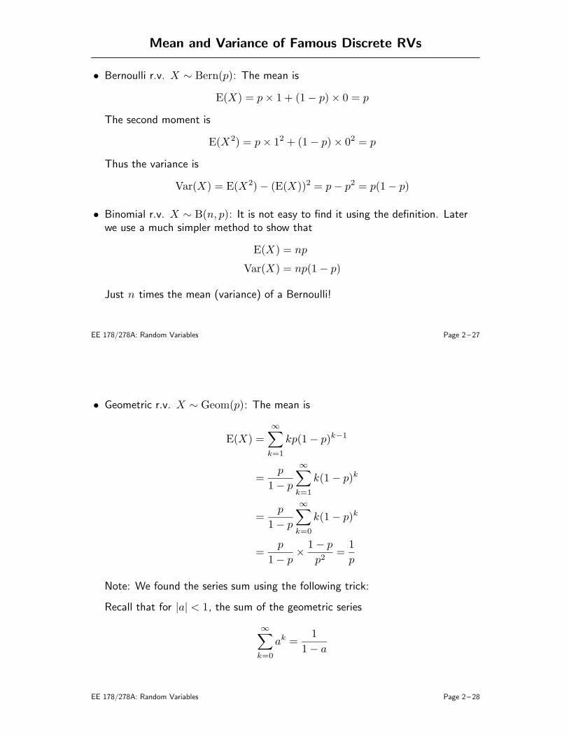
In fact the precise way to define a continuous random variable is through thecontinuity of its cdf Further, if FX(x) is differentiable (almost everywhere),then

fX(x) =dFX(x)

dx= lim

∆x→0

FX(x+∆x)− FX(x)

∆x

= lim∆x→0

Px < X ≤ x+∆x∆x

The cdf of a mixed r.v. has the general form

FX(x)

1

x


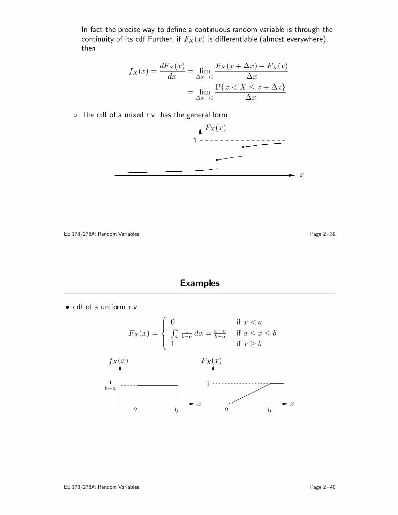
Examples

• cdf of a uniform r.v.:

FX(x) =

0 if x < a∫ x

a1

b−a dα = x−ab−a if a ≤ x ≤ b

1 if x ≥ b

fX(x) FX(x)

1b−a

a a bbxx

1


• cdf of an exponential r.v.:

FX(x) = 0, X < 0, and FX(x) = 1− e−λx, x ≥ 0

fX(x) FX(x)

λ 1

xx


• cdf for a mixed r.v.: Let X be the service time of a packet at a router. If thebuffer is empty (happens with probability p), the packet is serviced immediately.If it is not empty, service time is described by an exponential pdf with parameterλ > 0

The cdf of X is

FX(x) =

0 if x < 0p if x = 0p+ (1− p)(1− e−λx) if x > 0

FX(x)

p

1

x


• cdf of a Gaussian r.v.: There is no nice closed form for the cdf of a Gaussianr.v., but there are many published tables for the cdf of a standard normal pdfN (0, 1), the Φ function:

Φ(x) =

∫ x

−∞

1√2π

e−ξ2

2 dξ

More commonly, the tables are for the Q(x) = 1− Φ(x) function

N (0, 1)

x

Q(x)

Or, for the complementary error function: erfc(x) = 2Q(√2x) for x > 0

As we shall see, the Q(·) function can be used to quickly compute PX > afor any Gaussian r.v. X


Functions of a Random Variable

• We are often given a r.v. X with a known distribution (pmf, cdf, or pdf), andsome function y = g(x) of x, e.g., X2, |X |, cosX , etc., and wish to specify Y ,i.e., find its pmf, if it is discrete, pdf, if continuous, or cdf

• Each of these functions is a random variable defined over the originalexperiment as Y (ω) = g(X(ω)). However, since we do not assume knowledgeof the sample space or the probability measure, we need to specify Y directlyfrom the pmf, pdf, or cdf of X

• First assume that X ∼ pX(x), i.e., a discrete random variable, then Y is alsodiscrete and can be described by a pmf pY (y). To find it we find the probabilityof the inverse image ω : Y (ω) = y for every y. Assuming Ω is discrete:

x1x2 x3 y1 y2 y . . .. . .. . .

g(xi) = y


pY (y) = Pω : Y (ω) = y

=∑

ω: g(X(ω))=y

Pω

=∑

x: g(x)=y

∑

ω: X(ω)=x

Pω =∑

x: g(x)=y

pX(x)

ThuspY (y) =

∑

x: g(x)=y

pX(x)

We can derive pY (y) directly from pX(x) without going back to the originalrandom experiment


• Example: Let the r.v. X be the maximum of two independent rolls of afour-sided die. Define a new random variable Y = g(X), where

g(x) =

1 if x ≥ 30 otherwise

Find the pmf for Y

Solution:

pY (y) =∑

x: g(x)=y

pX(x)

pY (1) =∑

x: x≥3

pX(x)

=5

16+

7

16=

3

4

pY (0) = 1− pY (1) =1

4


Derived Densities

• Let X be a continuous r.v. with pdf fX(x) and Y = g(X) such that Y is acontinuous r.v. We wish to find fY (y)

• Recall derived pmf approach: Given pX(x) and a function Y = g(X), the pmfof Y is given by

pY (y) =∑

x: g(x)=y

pX(x),

i.e., pY (y) is the sum of pX(x) over all x that yield g(x) = y

• Idea does not extend immediately to deriving pdfs, since pdfs are notprobabilities, and we cannot add probabilities of points

But basic idea does extend to cdfs


• Can first calculate the cdf of Y as

FY (y) = Pg(X) ≤ y

=

∫

x: g(x)≤y

fX(x) dx

x y

y

x : g(x) ≤ y

• Then differentiate to obtain the pdf

fY (y) =dFY (y)

dy

The hard part is typically getting the limits on the integral correct. Often theyare obvious, but sometimes they are more subtle


Example: Linear Functions

• Let X ∼ fX(x) and Y = aX + b for some a > 0 and b. (The case a < 0 is leftas an exercise)

• To find the pdf of Y , we use the above procedure

y

x

y

y−ba


FY (y) = PY ≤ y = PaX + b ≤ y

= P

X ≤ y − b

a

= FX

(

y − b

a

)

Thus

fY (y) =dFY (y)

dy=

1

afX

(

y − b

a

)

• Can show that for general a 6= 0,

fY (y) =1

| a |fX(

y − b

a

)

• Example: X ∼ Exp(λ), i.e.,

fX(x) = λe−λx, x ≥ 0

Then

fY (y) =

λ|a|e

−λ(y−b)/a if y−ba ≥ 0

0 otherwise


• Example: X ∼ N (µ, σ2), i.e.,

fX(x) =1√2πσ2

e−

(x−µ)2

2σ2

Again setting Y = aX + b,

fY (y) =1

| a |fX(

y − b

a

)

=1

| a |1√2πσ2

e−

(

y−ba −µ

)2

2σ2

=1

√

2π(aσ)2e−

(y−b−aµ)2

2a2σ2

=1

√

2πσ2Y

e−

(y−µY )2

2σ2Y for −∞ < y < ∞

Therefore, Y ∼ N (aµ+ b, a2σ2)


This result can be used to compute probabilities for an arbitrary Gaussian r.v.from knowledge of the distribution a N (0, 1) r.v.

Suppose Y ∼ N (µY , σ2Y ) and we wish to find PY > y

From the above result, we can express Y = σYX + µY , where X ∼ N (0, 1)

Thus

PY > y = PσYX + µY > y

= P

X >y − µY

σY

= Q

(

y − µY

σY

)


Example: A Nonlinear Function

• John is driving a distance of 180 miles at constant speed that is uniformlydistributed between 30 and 60 miles/hr. What is the pdf of the duration of thetrip?

• Solution: Let X be John’s speed, then

fX(x) =

1/30 if 30 ≤ x ≤ 60

0 otherwise,

The duration of the trip is Y = 180/X


To find fY (y) we first find FY (y). Note that y : Y ≤ y = x : X ≥ 180/y,thus

FY (y) =

∫ ∞

180/y

fX(x) dx

=

0 if y ≤ 3∫ 60

180/yfX(x) dx if 3 < y ≤ 6

1 if y > 6

=

0 if y ≤ 3

(2− 6y) if 3 < y ≤ 6

1 if y > 6

Differentiating, we obtain

fY (y) =

6/y2 if 3 ≤ y ≤ 6

0 otherwise


Monotonic Functions

• Let g(x) be a monotonically increasing and differentiable function over its range

Then g is invertible, i.e., there exists a function h, such that

y = g(x) if and only if x = h(y)

Often this is written as g−1. If a function g has these properties, then g(x) ≤ yiff x ≤ h(y), and we can write

FY (y) = Pg(X) ≤ y= PX ≤ h(y)= FX(h(y))

=

∫ h(y)

−∞

fX(x) dx

ThusfY (y) =

dFY (y)

dy= fX(h(y))

dh

dy(y)


• Generalizing the result to both monotonically increasing and decreasingfunctions yields

fY (y) = fX(h(y))

∣

∣

∣

∣

dh

dy(y)

∣

∣

∣

∣

• Example: Recall the X ∼ U[30, 60] example with Y = g(X) = 180/X

The inverse is X = h(Y ) = 180/Y

Applying the above formula in region of interest Y ∈ [3, 6] (it is 0 outside) yields

fY (y) = fX(h(y))

∣

∣

∣

∣

dh

dy(y)

∣

∣

∣

∣

=1

30

180

y2

=6

y2for 3 ≤ y ≤ 6


• Another Example:

Suppose that X has a pdf that is nonzero only in [0, 1] and defineY = g(X) = X2

In the region of interest the function is invertible and X =√Y

Applying the pdf formula, we obtain

fY (y) = fX(h(y))

∣

∣

∣

∣

dh

dy(y)

∣

∣

∣

∣

=fX(

√y)

2√y

, for 0 < y ≤ 1

• Personally I prefer the more fundamental approach, since I often forget thisformula or mess up the signs


Documents

LectureNotes2 RandomVariables - Stanford Universityisl.stanford.edu/~abbas/ee178/lect02-2.pdf · • Why do we need random variables? Random variable can represent the gain or loss