Embed Size (px)
Citation preview
v2020
1 / 7
Biomathematics 2
Probability, random variables.
Continuous random variable. Normal, standard normal
distribution.
Dr. Beáta Bugyi
associate professor
University of Pécs, Medical School
Department of Biophysics
2020
v2020
2 / 7
CONTINUOUS RANDOM VARIABLE continuous: uncountable, infinite number of values, arises from measurement
Probability – discrete/continuous random variables
Let’s consider that a statistical experiment has an outcome corresponding to
A) a discrete random variable and X = 0 – 10 (finite number of outcomes: 10)
Give the probability that the outcome is 6.
𝑃(𝑋 = 6) =1
10= 0.1
B) a continuous random variable and X = 0 – 10 (infinite number of outcomes)
Give the probability that the outcome is 6. Exactly 6, not 6.1, 6.01, …, 6.00000000001
𝑃(𝑋 = 6) =1
∞= 0
NORMAL DISTRIBUTION
𝑁(𝜇, 𝜎), 𝜇 = 𝑚𝑒𝑎𝑛, 𝜎 = 𝑠𝑡𝑎𝑛𝑑𝑎𝑟𝑑 𝑑𝑒𝑣𝑖𝑎𝑡𝑖𝑜𝑛
Probability density function (PDF)
𝑓(𝑥) =1
√2𝜋𝜎2exp (−
(𝑥 − 𝜇)2
2𝜎2 )
Cumulative density function (CDF)
𝐹(𝑥) = ∫1
√2𝜋𝜎2exp (−
(𝑥 − 𝜇)2
2𝜎2 )𝑥
−∞
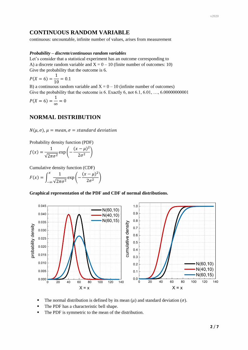
Graphical representation of the PDF and CDF of normal distributions.
The normal distribution is defined by its mean (𝜇) and standard deviation (𝜎).
The PDF has a characteristic bell shape.
The PDF is symmetric to the mean of the distribution.
v2020
3 / 7
The inflection point of the PDF corresponds to the standard deviation of the distribution.
The width (width at half-maximum) of the PDF is proportional to the standard deviation; the
larger the width the larger the standard deviation.
Probability is given by the area under the PDF (see examples below).
Example 1
The test result of students from Subject 1 follows a normal distribution with a mean of 60% and
standard deviation of 10%. 𝑵(𝝁, 𝝈) = 𝑵(𝟔𝟎, 𝟏𝟎). Represent graphically the following
probabilities.
Q1.1: What is the probability that a student scores 60%? 𝑃(𝑋 = 𝑥 = 60) = ?
Q1.2: What is the probability that a student scores less than 60%? 𝑃(𝑋 < 𝑥 = 60) =?
Q1.3: What is the probability that a student scores more than 60%? 𝑃(𝑋 > 𝑥 = 60) = ?
Q1.4: What is the probability that a student scores less than 80%? 𝑃(𝑋 < 𝑥 = 80) = ?
Q1.5: What is the probability that a student scores between 60% and 80%? 𝑃(𝑥 = 60 < 𝑋 < 𝑥 =
80) = ?
Example 2
The test result of students from Subject 2 follows a normal distribution with a mean of 62% and
standard deviation of 8%. 𝑵(𝝁, 𝝈) = 𝑵(𝟔𝟐, 𝟖).
Question:
How can we work with different normal distributions? Do we need the PDF of each and every normal
distribution?
Answer:
Normal distributions can be standardized; ∞ normal distribution 1 standardized distribution
(standard normal distribution)
How to standardize normal distributions?
𝑁(𝜇, 𝜎)
z score: 𝒛 =𝒙−𝝁
𝝈
z score: how many standard deviations (𝜎) is a given value (𝑥) from the mean (𝜇)
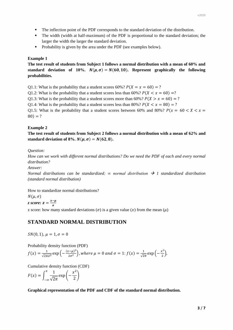
STANDARD NORMAL DISTRIBUTION
𝑆𝑁(0, 1), 𝜇 = 1, 𝜎 = 0
Probability density function (PDF)
𝑓(𝑥) =1
√2𝜋𝜎2exp (−
(𝑥−𝜇)2
2𝜎2 ) , 𝑤ℎ𝑒𝑟𝑒 𝜇 = 0 𝑎𝑛𝑑 𝜎 = 1: 𝑓(𝑥) =1
√2𝜋exp (−
𝑥2
2),
Cumulative density function (CDF)
𝐹(𝑥) = ∫1
√2𝜋exp (−
𝑥2
2)
𝑥
−∞
Graphical representation of the PDF and CDF of the standard normal distribution.
v2020
4 / 7
Z table
summarizes the CDF of the standard normal distribution
Example 1
The test result of students from Subject 1 follows a normal distribution with a mean of 60% and
standard deviation of 10%. 𝑵(𝝁, 𝝈) = 𝑵(𝟔𝟎, 𝟏𝟎). Standardize the normal distribution. Give the
probabilities by using the Z table.
Q1.1: What is the probability that a student scores 60%? 𝑃(𝑋 = 𝑥 = 60) = ?
𝑃(𝑋 = 𝑥 = 60) = 0
Q1.2: What is the probability that a student scores less than 60%? 𝑃(𝑋 < 𝑥 = 60) =?
𝑧 =𝑥 − 𝜇
𝜎=
60 − 60
10= 0.00
𝑃(𝑋 < 𝑥 = 60) = 0.5 → 50 %
Q1.3: What is the probability that a student scores more than 60%? 𝑃(𝑋 > 𝑥 = 60) = ?
𝑃(𝑋 > 𝑥 = 60) + 𝑃(𝑋 < 𝑥 = 60) = 1
𝑃(𝑋 > 𝑥 = 60) = 1 − 𝑃(𝑋 < 𝑥 = 60) = 1 − 0.5 = 0.5 → 50 %
Q1.4: What is the probability that a student scores less than 80%? 𝑃(𝑋 < 𝑥 = 80) = ?
𝑧 =𝑥 − 𝜇
𝜎=
80 − 60
10= 2.00
𝑃(𝑋 < 𝑥 = 80) = 0.9772 → 97.72 %
Q1.5: What is the probability that a student scores between 60% and 80%? 𝑃(𝑥 = 60 < 𝑋 < 𝑥 =
80) = ?
𝑃(𝑋 < 80) − 𝑃(𝑋 < 60) = 0.9772 − 0.5 = 0.4772 → 47.72%
Example 2
v2020
5 / 7
The test result of students from Subject 2 follows a normal distribution with a mean of 62% and
standard deviation of 8%. 𝑵(𝝁, 𝝈) = 𝑵(𝟔𝟐, 𝟖). Give the probabilities by using the Z table.
Q2.1: What is the probability that a student scores less than 65%? 𝑃(𝑋 < 𝑥 = 65) =?
𝑧 =𝑥 − 𝜇
𝜎=
65 − 62
8= + 0.375
If a value is not listed in the table, use the following approximation:
+ 0.375 =0.37 + 0.38
2
𝑃(𝑋 < 𝑥 = 65) =0.6443 + 0.6480
2= 0.6462 → 64.62 %
Q2.2: What is the probability that a student scores less than 45%? 𝑃(𝑋 < 𝑥 = 45) =?
𝑧 =𝑥 − 𝜇
𝜎=
45 − 62
8= −2.125
If a value is not listed in the table, use the following approximation:
−2.125 =−2.12 + (−2.13)
2
𝑃(𝑋 < 𝑥 = 45) =0.0170 + 0.0166
2= 0.0168 → 1.68 %
Q2.3: What is the probability that a student scores between 45% and 65%? 𝑃(𝑥 = 45 < 𝑋 < 𝑥 = 65) =
?
𝑃(𝑥 = 45 < 𝑋 < 𝑥 = 65) = 𝑃(𝑋 < 𝑥 = 65) − 𝑃(𝑋 < 𝑥 = 45) = 0.6462 − 0.0168 = 0.6294
→ 62.94 %
Q2.4: What is the median of the students’ scores? 𝑃(𝑋 < 𝑥) = 0.5, 𝑥 = ?
𝑃(𝑋 < 𝑥) = 0.5 → 𝑧 = 0.00
𝑧 =𝑥 − 𝜇
𝜎→ 0.00 =
𝑥 − 62
8→ 𝑥 = 62
Note: The mean of a data set following normal distribution is equal to its median.
Q2.5: What is the first quartile of the students’ scores? 𝑃(𝑋 < 𝑥) = 0.25, 𝑥 = ?
𝑃(𝑋 < 𝑥) = 0.25 → 𝑧 = −0.675
𝑧 =𝑥 − 𝜇
𝜎→ −0.675 =
𝑥 − 62
8→ 𝑥 = 56.6
Q2.6: What is the third quartile of the students’ scores? 𝑃(𝑋 < 𝑥) = 0.75, 𝑥 = ?
𝑃(𝑋 < 𝑥) = 0.75 → 𝑧 = 0.675
𝑧 =𝑥 − 𝜇
𝜎→ 0.675 =
𝑥 − 62
8→ 𝑥 = 67.4
Q2.7: Find what percentage of data is between mean ± 1×standard deviation, mean ± 2×standard
deviation, mean ± 3×standard deviation.
v2020
6 / 7
IMPORTANCE OF NORMAL DISTRIBUTION
CENTRAL LIMIT THEOREM
Example 3
In a population of persons let X = life expectancy of a person (in years). The distribution of X
has a mean and standard deviation of 72 and 18.2 years, respectively.
𝑋 = 𝑙𝑖𝑓𝑒 𝑒𝑥𝑝𝑒𝑐𝑡𝑎𝑛𝑐𝑦 𝑜𝑓 𝑎 𝑝𝑒𝑟𝑠𝑜𝑛 𝑖𝑛 𝑎 𝑝𝑜𝑝𝑢𝑙𝑎𝑡𝑖𝑜𝑛 (𝑦𝑒𝑎𝑟𝑠)
𝑋 = 𝑥𝑝𝑒𝑟𝑠𝑜𝑛1, 𝑥𝑝𝑒𝑟𝑠𝑜𝑛2, …
We choose samples from the population, each of the samples consists of n persons and by
finding the average lifetime in each sample (�̅�, sample mean) we obtain the distribution of �̅�.
Sampling distribution of sample means: a distribution of the sample means calculated from all
possible random samples of a specific size (n) taken from a population.
�̅� = 𝑎𝑣𝑒𝑟𝑎𝑔𝑒 𝑙𝑖𝑓𝑒 𝑒𝑥𝑝𝑒𝑐𝑡𝑎𝑛𝑐𝑦 𝑜𝑓 𝑝𝑒𝑟𝑠𝑜𝑛𝑠 𝑖𝑛 𝑎 𝑠𝑎𝑚𝑝𝑙𝑒 (𝑦𝑒𝑎𝑟𝑠)
�̅� = �̅�𝑠𝑎𝑚𝑝𝑙𝑒1, �̅�𝑠𝑎𝑚𝑝𝑙𝑒2, …
Properties of the distribution of the sample means
𝜇�̅� = 𝜇𝑋
𝜎�̅� =𝜎𝑋
√𝑛 (standard error of the mean, SEM)
Characteristics of the distribution: Central limit theorem (CLT)
POPULATION SAMPLE
𝑋 = 𝑥
life expectancy of a person in a
population
�̅� = �̅�
average life expectancy of persons in a
sample
normal distribution normal distribution for any n
not normal/not known distribution
CLT: if n is large enough (𝑛 ≥ 30)
approximated by normal distribution
the larger n, the better the approximation
http://onlinestatbook.com/stat_sim/sampling_dist/index.html
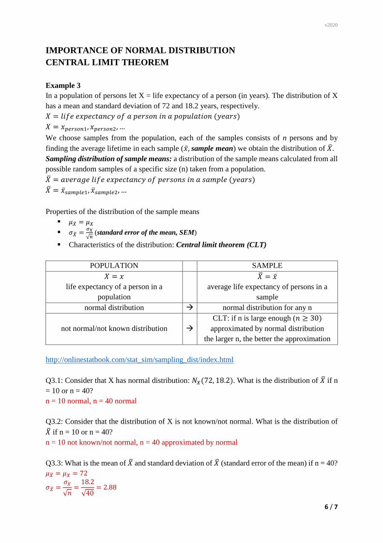
Q3.1: Consider that X has normal distribution: 𝑁𝑋(72, 18.2). What is the distribution of �̅� if n
= 10 or n = 40?
n = 10 normal, n = 40 normal
Q3.2: Consider that the distribution of X is not known/not normal. What is the distribution of
�̅� if n = 10 or n = 40?
n = 10 not known/not normal, n = 40 approximated by normal
Q3.3: What is the mean of �̅� and standard deviation of �̅� (standard error of the mean) if n = 40?
𝜇�̅� = 𝜇𝑋 = 72
𝜎�̅� =𝜎𝑋
√𝑛=
18.2
√40= 2.88
v2020
7 / 7
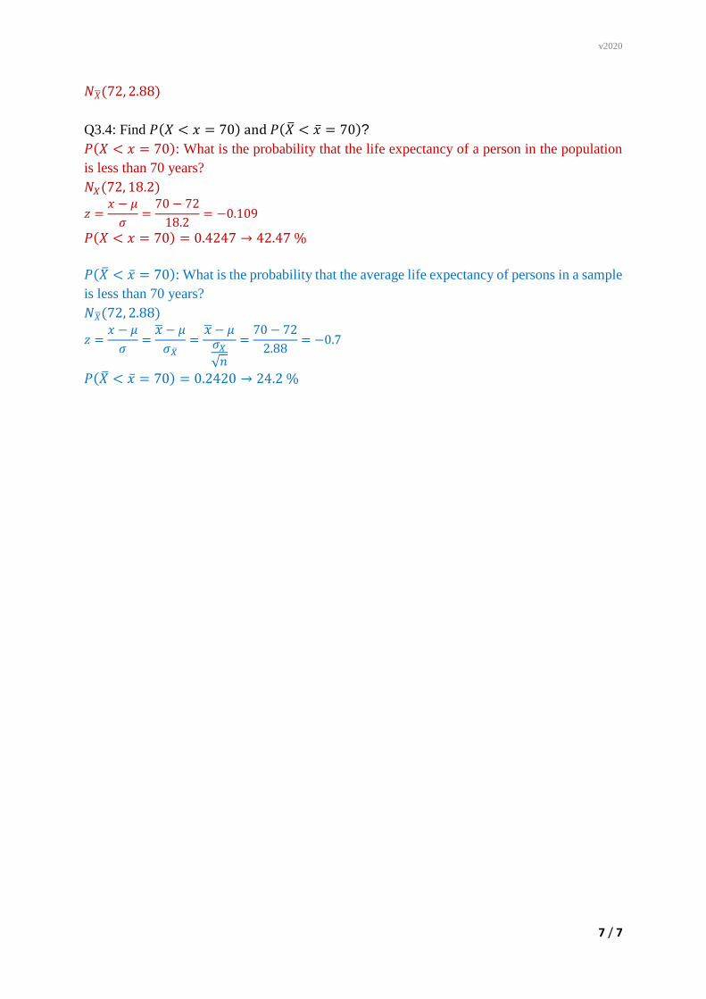
𝑁�̅�(72, 2.88)
Q3.4: Find 𝑃(𝑋 < 𝑥 = 70) and 𝑃(�̅� < �̅� = 70)?
𝑃(𝑋 < 𝑥 = 70): What is the probability that the life expectancy of a person in the population
is less than 70 years?
𝑁𝑋(72, 18.2)
𝑧 =𝑥 − 𝜇
𝜎=
70 − 72
18.2= −0.109
𝑃(𝑋 < 𝑥 = 70) = 0.4247 → 42.47 %
𝑃(�̅� < �̅� = 70): What is the probability that the average life expectancy of persons in a sample
is less than 70 years?
𝑁�̅�(72, 2.88)
𝑧 =𝑥 − 𝜇
𝜎=
�̅� − 𝜇
𝜎�̅�=
�̅� − 𝜇𝜎𝑋
√𝑛
=70 − 72
2.88= −0.7
𝑃(�̅� < �̅� = 70) = 0.2420 → 24.2 %