Embed Size (px)
Citation preview

1
PATHOGEN SURVEILLANCE:Designs and Analyses
University of TennesseeCenter for Wildlife Health
Department of Forestry, Wildlife and Fisheries
Matthew J. Gray
Lecture Outline
I. Uses of Surveillance Data
II. Statistical Inference
III. Sample Size and Sample Design
IV. Confidence Intervals and Tests

2
Goal of Pathogen Surveillance
To obtain an unbiased estimate of pathogen or disease prevalence in a populationor disease prevalence in a population
Pathogen Prevalence
An estimate of the proportion of individuals in aAn estimate of the proportion of individuals in a population that are infected with a pathogen
Infection Disease
Uses of Surveillance DataOccurrence and Distribution
Evidence of EmergencePathogen or disease that is increasing in
distribution, prevalence, or host range
3
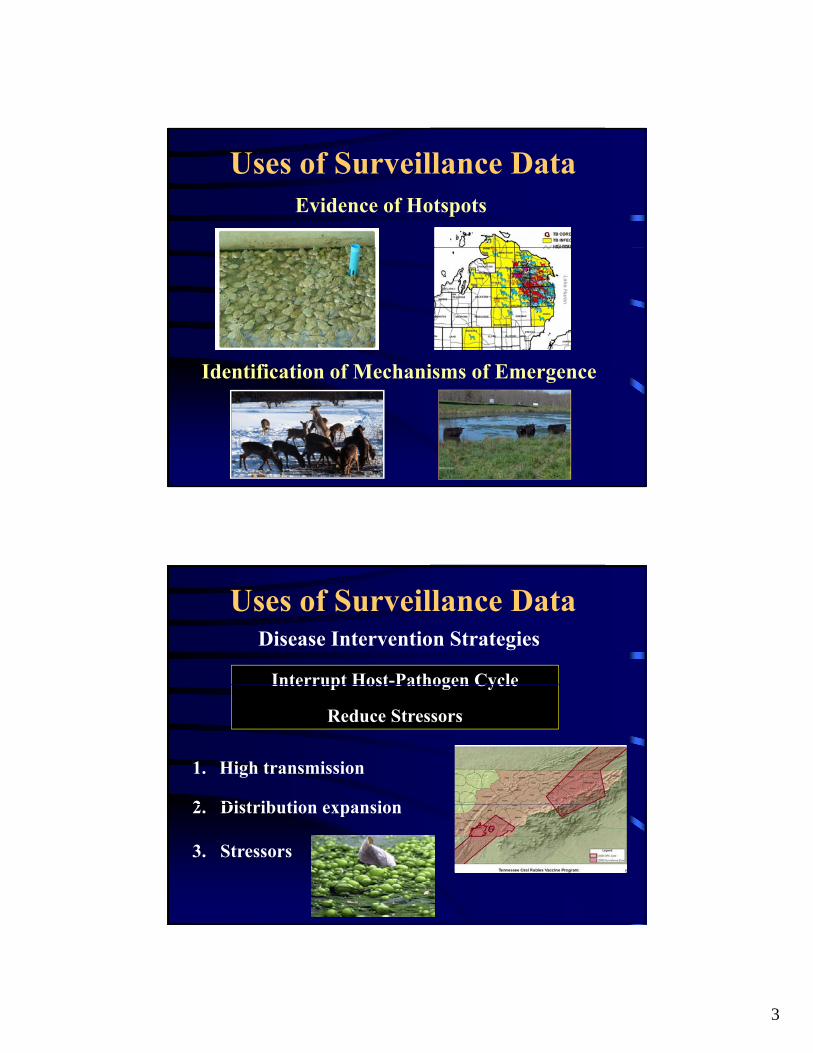
Uses of Surveillance DataEvidence of Hotspots
Id tifi ti f M h i f EIdentification of Mechanisms of Emergence
Uses of Surveillance DataDisease Intervention Strategies
Interrupt Host-Pathogen Cycle
1. High transmission
2 Distribution expansion
Interrupt Host Pathogen Cycle
Reduce Stressors
2. Distribution expansion
3. Stressors

4
Individual vs. Population
What conclusions can be made?What conclusions can be made?
Uses and Benefits of Individual vs. Population Data?
Statistical Inference on Populations
Population Sample
Subset of all individuals
Sample
σμ,P, S0 p
“Field of Statistics” “Point Estimates”
Is statistics necessary for reports on individual cases?
“Parameters”

5
Measures of Reliability
How variableHow close is
ti tHow variable is your
estimate?
your estimate a the true
prevalence?
S σ
Pp
numerical closeness of measurements to each other
numerical closeness of measurements to a true population parameter (P)
unbiased + precision
P•Precision:
•Bias:
•Accuracy:
Surveillance Designs
Random Sampling
All i di id l ill
Collecting Unbiased, Representative Sample
All individuals or surveillance locations have an equal
probability of being sampled
Random Numbers Table or Programs
Stratified Random Sampling
Habitat Type/Condition; Gender; Age Class
All individuals within a specified location or category have an equal probability of being sampled

6
Surveillance DesignsSystematic SamplingIndividuals or locations in specified intervals have an equalspecified intervals have an equal probability of being sampled
Other Designs: Cluster sampling, Multi-stage sampling, Adaptive Sampling
Biased if Not a Uniform Distribution
Haphazard Sampling
Individuals are selected based on ease of access or in a way that does not follow an unbiased random process.
Case Studies: Inferences Limited to the Sample
Detect a Pathogen
Estimating Required Sample Size
Information Needed•Assumed Pathogen Prevalence Level (APPL)
•Estimated Host Population Size
•Confidence in detection (95%)
Population Size 10% APPL 5% APPL 2% APPL
501002505002000>100,000
202325262730
354550556060
5075110130145150
(Amos 1985, Thoesen 1994)

7
Precise Estimate of Prevalence
Estimating Required Sample Size
n p p
( )
.1
1 962 Prevalence from a
previous studyZα/2 =1.96 p =
n p pd
( )1 previous study
d = error in estimation(95% confidence)
“Error in Estimation” is the amount of error you are willing to tolerate in your estimate of prevalence
Error = 5% Error = 10% Error = 10%p = 85%
n
( . )( . )( . )
.0 85 0 15
1 96
0 05196
2
p = 85% p = unknown
n
( . )( . )( . )
.0 85 0 15
1 96
0 1049
2
n
( . )( . )
.0 25
1 96
0 1096
2
What happens if estimation error increases?
What happens if prevalence is near 0.5?0.01< P(1-p) < 0.25
Estimating Prevalence
pi
n
Ni p
14
4010%
N i
Sp q
nwhere q pi i
i i
, 1
Estimate of Precision
40
n
Expected Average Deviation in p-hat around PStandard Deviation, S:
CI p Si( . ( )95%) 1 96 For Large n, 95% Confidence Interval:

8
Estimating Prevalence and CI
Sp q
ni i p
in
Ni
i
CI p Si( . ( )95%) 1 96
Infection Data:
Age Class Infected Sampled P_Hat Q_Hat S EM Lower UpperJuv 9 35 0.2571 0.7429 0.0739 0.145 0.112 0.402Subadult 10 40 0.25 0.75 0.0685 0.134 0.116 0.384Adult_F 5 15 0.3333 0.6667 0.1217 0.239 0.095 0.572Adult_M 3 30 0.1 0.9 0.0548 0.107 -0.007 0.207
CI Juv P( ) . . 0 112 0 402
CI SA P( ) . . 0 116 0 384
CI F P( ) . . 0 095 0 572
CI M P( ) . 0 0 207
Is Prevalence Different Among Age Classes?
Estimating Confidence Intervals
Wilson Score Method
Small Sample Size or Prevalence = 0
Journal of the American Statistical Association 22:209-212
http://faculty.vassar.edu/lowry/prop1.html

9
Hypothesis TestingTwo Proportions
p p 1 2 X Yiff if Zp p
pqn n
1 2
1 2
1 1 pX Y
n n
1 2
Different if Z > 1.96
Age Class Infected Sampled P_i P_Hat sq(P*Q) SqRt Den Num Z
Juv 9 35 0.2571 0.1846 0.388 0.249 0.097 0.157 1.6279
.p
9 3
35 300 185
Z
0 257 0 10
0 185 0 8151
35
1
30
1 63. .
. .
.
Adult_M 3 30 0.1
P = 0.104
Hypothesis TestingTwo Proportions
Minitab

10
Hypothesis TestingMultiple Proportions: One Hypothesis
Prevalence Different among 4 Age Classes?
Chi-square Test of Homogeneity
g g
SAS®
Hypothesis TestingMultiple Proportions: Two Hypotheses
Prevalence Different among 2 Land Uses and 3 Seasons?
Logistic Regression
g
SAS®

11
ResultsCattle Land Use
and Season
7.7X More Likely!!
Bd SurveillanceNon-lethal Techniques: Brem et al. (2007)
Swabbing PreferredA. Cressler, USGS
Ad lt
Swab 5 times in 5 locations
A. Cressler,
• Rear feet (webbing)
• Inner thighs
• Ventral Abdomen
L
Adults:
USGSLarvae:
Swab Oral Cavity 5 times
Store in 70% EtOH

12
Ranavirus SurveillanceLethal Collection:Liver Preferred
St-Armour & Lesbarrères (2007)
Non-lethal Techniques: Gray et al. (2012)
Misclassification Decreases as
Disease P
n = 96 tadpoles
Lesbarrères (2007)
Progresses
Lethal followed by Tail
Toe Clips
False positive = 3%False negative = 7%
St-Armour & Lesbarrères (2007)
Greer and Collins (2007)
Questions??