Lecture Notes onIdentification Strategies

Štepán Jurajda

June 12, 2007

Abstract

These lecture notes cover several examples of identification strategiesused in various fields of economics. They are meant to provide some guid-ance for those students looking for an empirical topic for their dissertations.

Contents

1 Introduction . . . . . . . . . . . . . . . . . . . . . . . . . . . . . . . . . 32 Search for Variation . . . . . . . . . . . . . . . . . . . . . . . . . . . . . 32.1 Control for X . . . . . . . . . . . . . . . . . . . . . . . . . . . . . 52.2 Group-Level Variation and Identification . . . . . . . . . . . . . . 52.3 Identification of National Policy Effects . . . . . . . . . . . . . . . 92.4 Exogenous Variation (IV) . . . . . . . . . . . . . . . . . . . . . . 102.5 Identification Through Heteroscedasticity . . . . . . . . . . . . . . 11

3 ‘Natural’ Experiments . . . . . . . . . . . . . . . . . . . . . . . . . . . 123.1 Experimental Setup and Solution . . . . . . . . . . . . . . . . . . 123.2 Difference in Differences . . . . . . . . . . . . . . . . . . . . . . . 13

3.2.1 Fixed Effects . . . . . . . . . . . . . . . . . . . . . . . . . 153.2.2 IV DD . . . . . . . . . . . . . . . . . . . . . . . . . . . . . 15

3.3 Regression Discontinuity . . . . . . . . . . . . . . . . . . . . . . . 163.4 When Can Things Go Wrong? . . . . . . . . . . . . . . . . . . . . 17

3.4.1 Internal Validity . . . . . . . . . . . . . . . . . . . . . . . 183.4.2 External validity . . . . . . . . . . . . . . . . . . . . . . . 193.4.3 Possible Improvements . . . . . . . . . . . . . . . . . . . . 20

3.5 Testing Non-Experimental Methods . . . . . . . . . . . . . . . . . 204 Defining Goals for Policy Analysis . . . . . . . . . . . . . . . . . . . . . 215 Other Selected Methods . . . . . . . . . . . . . . . . . . . . . . . . . . 235.1 Oaxaca-Blinder Decompositions . . . . . . . . . . . . . . . . . . . 235.2 Meta Analysis . . . . . . . . . . . . . . . . . . . . . . . . . . . . . 245.3 Expectations . . . . . . . . . . . . . . . . . . . . . . . . . . . . . 25

6 References . . . . . . . . . . . . . . . . . . . . . . . . . . . . . . . . . . 25

2

1. Introduction

The ultimate goal of econometrics is to learn about causal relationships frommicrodata capturing non-experimental economic behavior. This is hard in principle be-cause social sciences differ from, e.g., medicine where (double-blind) randomizedexperiments are the way to learn. There are often elusive unobservables affectingthe outcome; hence, the need for sample selection (treatment assignment) con-trol. Economic processes often lead to simultaneity so that we need exogenous(experiment-like) variation. Econometrics differs from statistics in defining theidentification problem: structural and reduced-form equations.

Example 1.1. Suppose that you are interested in the effect of military service onsubsequent earnings. You can look at the mean difference in the outcome betweenveterans and non-vets. Inside this number hides not only a causal effect of theservice, but also the composition of other causal variables in each group, bothobserved and unobserved. Are there variables that affect both participation inthe program and the outcome? Are the (minority) vets earning more because ofthe military service or are the high-earners more likely to enroll in the army?

When we regress y = Xβ + ε to estimate bβ, we only sometimes mean thatX causes y. Often, we focus on the effect of one causal variable (for whichwe have an exogenous source of variation) and use other regressors as controlvariables. Often the causal variable captures some treatment (policy, trainingprogram, education, etc.). When asking about causal relationships, we wish toanswer “what if” questions (estimate the counterfactual).1 An alternative useof regression analysis is as a descriptive statistical tool. There is no behavioralmeaning to a conditional expectation such as

E[y|x] =Z ∞

−∞ydF (y|x).

2. Search for Variation

You need variation in x to estimate a coefficient. Where does it come from? In an“ignorant” research design, you simply take a dataset and estimate a coefficientusing whatever variation there is in the data, having controlled for other potential

1What would have happened to car accidents had we not lowered max speed to 50 km/h?What would happen if we shorten criminal sentences?

3

explanatory variables. Parameter estimates do not drop from heaven–they aredirectly the outcome of the potentially many sources of variation in your data.Some of these may be endogenous, and at least some of these you should be

able to understand and focus on in the estimation.

Example 2.1. Suppose that you compare crime rates and deterrence across Czechdistricts. Specifically, you regress district crime rates on district police force sizeper crime, after controlling for a district fixed effect. But this differences in de-terrence may actually largely come from different trends in regional crime ratescombined with even and fixed distribution of police force size inherited from com-munism. So it’s unclear to what extent we measure one way causality here.

Example 2.2. You want to regress age at first marriage on wages using RLMS,but you only see young women getting married if they still live with parents, whichis itself a function of labor income.

Different sources of variation lead to different interpretation of (different esti-mates of) the coefficients. For example, compare panel-data estimators based ononly the ‘within’ time change variation to those based on both time and cross-sectional variation.

Example 2.3. See Bell et al. (2002) for an application relating wages and un-employment in several dimensions: (i) aggregate time series, (ii) cross-sectionalcompensating wage differentials as a no-moving equilibrium, (iii) regional equili-bration conditional on time and regional fixed effects.

In any case, the variation giving rise to coefficient estimates should be linkedto the problem studied.

Example 2.4. You motivate a paper by comparing living with parents and em-ployment uncertainty for young workers across Italy and Sweden, but then youestimate the effect using within-Italy variation. Is it X or β?

In this section we look at some difficult identification situations and start withsome examples of where IVs come from. But first we say what we do in any case:

4

2.1. Control for X

Of course, before you start worrying about the sources of identification for yourvariable of interest, you should control for other variables that are correlated withyour causing variable. If you fail to find all of these, you need an IV.

Example 2.5. Returns to education, ability bias and IQ test scores.

When is controlling for X enough to identify a causal effect? I.e., when isselection on observables plausible? (When is it plausible that conditional on X,assignment to treatment is as good as random?)

Example 2.6. If applicants to a college are screened based on X, but conditionalon passing the X test, they are accepted based on a first-come/first-serve basis.

To control for X, run a regression or perform a matching exercise (when treat-ment is binary). The idea of matching is to compare the outcome y for individualsfrom the treatment and control groups for each value of X. Then average the dif-ference in the outcomes using the distribution of X for treatments to obtain theestimate of the treatment effect on those who got the training. A feasible wayto implement this strategy with multidimensional X is to condition on the unidi-mensional probability of treatment P (X) rather than on the multi-dimensional setof covariates X. The difference from a regression approach is in (i) the exclusionof comparisons where there is lack of common support, i.e., where certain P (X)values are not present in both groups, (ii) in the weights attached to the differencein outcome for each value of X, and (iii) in not imposing linearity.

2.2. Group-Level Variation and Identification

Often variation of interest in x does not occur across individuals but across groupsof individuals (firms, regions, occupations).

Inference When using individual-level data with group-level variation in thevariable of interest, one needs to correct standard errors to admit the actual num-ber of degrees of freedom (dimension of the variation of interest). This is done byincluding a random effect, a (block-diagonal-matrix) White/Huber heteroscedas-ticity correction (use cluster option in Stata), or by aggregating the data to theappropriate level (Bertrand et al., 2002). A potentially better approach of Don-ald and Lang (2000-2004), applicable especially when the number of groups (both

5

treatment and control) is small, is to follow a two step approach: first estimatean individual-level regression with fixed effects corresponding to the group-levelvariation and in the second stage run these fixed effects on the group-level RHSvariable.2 If the number of individuals within each group is large, this two-stepestimator is efficient and its t-statistics are distributed t if the underlying groupserrors are normally distributed. They even recommend running the first stageseparately for each group.

The Reflection Problem See Manski (1995). Sometimes you ask why indi-viduals belonging to the same group act in a similar way. Economists usuallythink this may be because their xi are similar or because the group has a commoncharacteristic zg (for example ethnic identity):

yig = α+ β0xig + γ

0zg + εig.

Sociologists add that an individual may act in some way because other individualswithin the group act that way, that is because of E[y|z] (herd behavior, contagion,norm effects; there is a social multiplier, an endogenous social effect) or becausethe individual outcome varies with the mean of the exogenous variables in thereference group E[x|z] (exogenous social effect).

Example 2.7. Does the propensity to commit crimes depend on the averagecrime rate in the neighborhood or on the average attributes of people living in theneighborhood or on some exogenous characteristics of the neighborhood like thequality of schools etc.? Or think of high-school achievement as another example.

Note that the regression

E[y|z, x] = α+ β0x+ γ

0z + δ

0E[y|z] + λ

0E[x|z] (2.1)

has a social equilibrium: taking an expectation of both sides w.r.t. x we get

E[y|z] = α+ β0E[x|z] + γ

0z + δ

0E[y|z] + λ

0E[x|z],

which you can solve for E[y|z] and plug back into equation 2.1 to show thatin the reduced form equation, in which E[y|z, x] depends on (1, E[x|z], z), the

2One can think of the second stage as a Minimum Distance problem (see Section ??) whereone ought to weight with the inverse of the variance of the estimated fixed effects. One may alsoneed to think about the different implied weighting in the individual- and group-level regressions,and about omitted variable bias (see, e.g., Baker and Fortin, 2001).

6

structural parameters are not identified. We cannot separately identify the so-called correlated, endogenous, and contextual effects. Under some conditions, wecan say if at least one of the social effects is present, but we cannot determinewhich one.One hope, see Borjas (1992), is to use assumptions about the dynamics of

social processes and to run

Et[y|z, x] = α+ βxt + γzt + δEt−1[y|z].

See also Durlauf (2002) who trashes the recent social-capital (SC) literatureby applying the same identification logic. He first considers an individual-levelregression of the following type

yig = α+ β0xig + γ

0zg + δE(yg|Fg) + θE(SCg|Fg) + εig. (2.2)

In his presentation, zg corresponds to the contextual effects (variables measured atgroup level predetermined at the the time of choice, such as averages of individualcharacteristics). If SCg is predetermined (E(SCg|Fg) = SCg), it is simply anothercontextual effect and identification requires the presence of at least one individual-level variable whose group level average does not causally affect individuals.If SCg is an endogenous outcome of decisions that are contemporary to the

behavioral choice yig, then one needs two elements of xig not to be elements ofzg so as to provide instruments for E(yg|Fg) and E(SCg|Fg). That is one needstwo individual characteristics that affect individual behavior yet whose groupanalogues are excluded from the behavioral equation 2.2. This results is basedon considering the two simultaneous equations: one determining y (equation 2.2),the other for SC :

SCig = α+ β0xig + γ

0zg + δE(yg|Fg) + θE(SCg|Fg) + ηig. (2.3)

Finally, Durlauf (2002) considers the case of having only aggregate (group-level) data. The system then boils down to:

yg = α+ γ0zg + δE(yg|Fg) + θE(SCg|Fg) + εg (2.4)

SCg = α+ γ0zg + δE(yg|Fg) + θE(SCg|Fg) + ηg. (2.5)

and identification is a textbook case asking whether one has instruments for thetwo endogenous variables E(yg|Fg) and E(SCg|Fg): Are there variables in this

7

world that would affect social capital formation but not other behavior (like GDPgrowth in Knack and Keefer, QJE 1997)?Brock and Durlauf (2001) show that the lack of identification between en-

dogenous and contextual effects does not occur in binary and multinomial choicemodels, essentially because of their non-linearity. Zanella (2007, JEEA) appliesthe nested logit structure to a random utility framework in order to build amodel with social interactions and endogenous choice of the group membership(neighborhood); the micro-founded model then suggests econometric identificationstrategies.

Movers vs. Averages When we do not have an IV, but the source of endo-geneity is time constant (alternatively, when the unobservable selection thresholdis time constant), we can use a fixed effect panel data model to deal with it. Also,when comparing an outcome y across groups, one may be worried that there aredifferences in the average level of unobservables across the groups.

Example 2.8. Consider studying the wage effects of union/non-union status or ofgender segregation (concentration of women in occupations). Instead of comparinglevels, you can compare changes (run the fixed effect model). How does the unionstatus or the female fraction of workers in an occupation change? This strategyis thought of as being closer to causal evidence; it relies on “movers” – but arethey exogenous?

Consider the effect of a union dummy (0/1 variable) in levels and in firstdifferences:

yit = UNIONitβ + it

yit − yit−1 = (UNIONit − UNIONit−1)β +4 it

and note that only those who switch status between t and t − 1 are used in the‘difference’ estimation. A similar argument can be made when using aggregatedata.3

3For example, if you want to study the effect of part-time work on fertility, you can hardly runfertility on part-time status of individuals and pretend part-time status is assigned exogenously.But perhaps, if there is variation across regions and time in availability of part-time jobs, onecould estimate a relationship at the aggregate level.

8

Example 2.9. Gould and Paserman (2002) ask if women marry later when malewage inequality increases. They use variation across U.S. cities in male wageinequality and marriage behavior and allow for city-specific fixed effects and timetrends to establish causality. To write a paper like this, start with graphs of levelsand changes, then condition on other X variables, check if female wage inequalityhas any effect (it doesn’t), and conclude. It is not clear where changes in malewage inequality come from, but one would presumably not expect these changesto be driven by a factor that would also affect marriage behavior.

2.3. Identification of National Policy Effects

In case of national policy changes, within-country identifying variation is hardto come by while cross-country variation is often plagued by country-level unob-servables. Some examples of within-country as well as across-country approachesfollow.

Differences in take up compliance Ham et al. (1998) estimate the unem-ployment insurance effect on durations using a national system. Max and minare not enough. First, try to compare non-recipients and recipients, but this isrejected by a LR test. Fortunately some workers register late after loosing job.

Pre-policy distance from policy level Manning (2001) studies a nationalincrease in minimum wages by relating changes in employment before and afterthe minimum wage introduction to the fraction of low paid workers in the pre-minimum wage period. See also a classic paper by Card (1992) who considers theimposition of a federal minimum wage: the “treatment effect” varies across statesdepending on the fraction of workers initially earning less than the new minimum.Paligorova (2007) compares the effect of Sarbanes Oxley through company boardindependence for those companies that did not have independent board as of be-fore the act and those that did. She first shows that those that did not haveindependent board do indeed show a stronger increase in independence in com-parison to those firm that did have independent boards as of before SOX. This isstep 0 in all of program evaluation: establish that there is a program!

Cross-country indirect strategies It is usually hard to use country-wide be-fore/after and cross-country comparisons to identify national policy effects. See,e.g., the discussion of identifying effects of institutions in Freeman (1998). But

9

avoiding the main identification issue and focusing on interactions of the maincausal variable can shed some light on the direction and mechanism of the causaleffect.Rajan and Zingales (1998, JF) study the finance-growth nexus. One should

isolate the part of the variation in financial development that is unrelated to cur-rent and future growth opportunities, which are inherently unobservable. Tacklingthis identification problem at the country level is very difficult. So, Rajan andZingales (1998) give up on the big question and provide qualitative evidence oncausality using industry-country comparisons. They come up with an industry-specific index of the need for tapping the financial system (using external finance)and regress industry growth from a sample of countries on country and global-industry fixed effects as well as on the interaction between U.S. industry externalfinance dependence (EFD) and country financial development. Such regressionasks whether industries predicted to be in more need of external finance growfaster in countries with more developed financial markets, conditional on all (po-tentially unobservable) country- and industry-specific factors driving growth.

2.4. Exogenous Variation (IV)

You want to estimate β in y = Xβ + ε but E[ε|X] 6= 0 because of endogeneityor measurement error. A valid instrument Z is correlated with X but not withε. The R2 of the first stage should not be too high or too low. Where do you getsuch a variable? One solution is to find a “natural” experiment (more correctlyquasi-experiment) which generates such variation and then rely on this one sourcealone (read Angrist and Krueger, 2001, for a reader-friendly exposition). Theestimation designs/techniques are discussed in the next section.

Example 2.10. Card (1993) estimates returns to schooling, which may be af-fected by ability endogeneity bias, using proximity to college as an instrument foreducation. You may think of the distribution of student distance from college asproviding a quasi experiment that the regression is using. Ideally, you want todrop students randomly from helicopter. Is this case close enough? Whose effectare we estimating?

Example 2.11. Changes in wage structure, which occur in a supply-demandframework: “Women, War and Wages” by Acemoglu, Autor and Lyle. First,establish that there is a treatment–variation in draft causes differences in femalelabor supply. Second, ask whether there is an effect–of female labor supply onwage dispersion.

10

Remark 1. Testing validity of IV: There are two issues: (a) testing for whetherIV is exogenous (COV (ε, Z) = 0), and (b) testing for the weak instrument problem(COV (X,Z) 6= 0). IV is an asymptotic estimator, unlike OLS which is unbiasedin small samples.

Remark 2. Other than econometric tests for IV validity (see Econometrics IV)there are also intuitive tests in situations when identification comes from somequasi-experiment. For example, ask whether there is an association between theinstrument and outcomes in samples where there should be none.

Remark 3. See Berg 2007, IZA DP No. 2585 for a discussion of IVs, whichderive from the time interval between the moment the agent realizes that theymay be exposed to the policy and the actual exposure. Berg presents an economicmodel in which agents with larger treatment status have a stronger incentive tofind out about the value of the IV, which invalidates the IV. In other words,the exclusion restriction is likely to be violated if the outcome depends on theinteraction between the agent’s effort and his treatment status.

2.5. Identification Through Heteroscedasticity

A completely different approach to identification working off second moments:Hogan and Rigobon (2002). Estimate returns to education when education isendogenous by splitting the sample into two groups based on different covariancematrices. They suggest this strategy is stronger when compared to IV becauseIVs are weak and there is a lot of variance in heteroscedasticity, so one can useit to solve measurement error, simultaneity and omitted variable biases in cross-sectional data.As an illustration consider a model for wages w and schooling s

wi = βsi +Xiμ1 + i

si = αwi +Xiμ2 + ηi.

The covariance of the reduced form, which we can estimate,

Ω =1

(1− αβ)2

∙ν + β2νη αν + βνη

· α2ν + νη

¸,

consists of 3 equations in 4 unknowns (ν , νη, α, β). Now, suppose you split thesample into two parts, which have empirically different Ω. If the regression coef-ficients are stable across groups, suddenly you have 6 equations in 6 unknowns.

11

The crucial condition for this approach to be credible is to find a situationwhere coefficients are stable across sub-populations with different variances. Un-like in the natural-experiment literature, here it is harder to explain the economicmeaning behind the identification.

3. ‘Natural’ Experiments

Meyer (1995) and Angrist and Krueger (1999): “Natural experiment” examineoutcome measures for observations in treatment groups and comparison (control)groups that are not randomly assigned. In absence of randomization, we look forsources of variation that resemble an experimental design.

Example 3.1. For example, when studying the effect of unemployment benefitson labor supply, it is hard to differentiate the effect of the benefits from the effect ofpast labor supply and earnings. So a quasi-experimental design would use changesin benefits applying to some groups but not others (benefits such as maternitybenefits, unemployment insurance, workers’ compensation, Medicaid, AFDC) todefine the treatment and control groups.

Example 3.2. Other examples of quasi-experimental variation: Vietnam-era draftlottery, state-level minimum wage laws changes, large influxes of immigrants, fam-ily size effect on family choice and the delivery of twins, the variation in numberof children coming from the gender sequence of children (preference for a boy),returns to education and quarter of birth (compulsory schooling), differential dis-tance in effect of medical treatment (heart disease). Think of these events asproviding an IV.4

3.1. Experimental Setup and Solution

Consider a study of the effect of a training program where workers are randomizedinto and out of treatment (training). The effect of the program: y1i is earningwith training, y0i is earnings without training. We only look at the populationof eligible workers. They first choose to apply for the training program or not.We observe y1i only when Di = 1 (the person applied for and took training) andobserve y0i only when Di = 0 (these are the so called eligible non-participants,

4Similarly, if there is a random assignment to treatment, but imperfect compliance, theassignment indicator is the right IV for the treatment dummy.

12

ENPs). We want to knowE[y1i−y0i]. We also want to knowE[y1i−y0i|Di = 1], theeffect of treatment on treated, TT. However, the data only provides E[y1i|Di = 1]and E[y0i|Di = 1] is not observed–it is the counterfactual. This problem issolved by randomization: take the D = 1 group and randomize into treatment(R = 1) and control (R = 0) group. Then construct the experimental outcome:E[y∗1i|D∗

i = 1, Ri = 1]−E[y∗0i|D∗i = 1, Ri = 0].

5

Remark 4. However, experiments are costly, often socially unacceptable (in Eu-rope), and people may behave differently knowing they are in an experiment (thinkof expanding medical coverage).6

Remark 5. See Kling NBER WP no. 12931 for a guide to recent advances inusing field experiments in public finance.

3.2. Difference in Differences

A simple research resign, referred to as “Differences,” compares one group be-fore and after the treatment (i.e., employment before and after minimum wageincrease): yit = α + βdt + εit, where dit ∈ 0, 1 is the dummy for the treatmentgroup. The crucial assumption is that without treatment, β would be 0 (no dif-ference in means of y for treatment and control (before and after) groups). Soestimate of beta is just mean of y after minus mean of y before. If there arechanges in other conditioning variables, add x

0itγ. However, there are often under-

lying trends and/or other possible determinants (not captured by x) affecting theoutcome over time, making this identification strategy rather weak.Therefore, a very popular alternative is the “Difference in differences” design,

that is a before/after design with an untreated comparison group. Here, we havea treatment (j = 1) and a comparison (j = 0) group for both the before (t = 0)and after (t = 1) time period:

yjit = α+ α1dt + αjdj + βdjt + γ0xjit + εjit

βDD = y11 − y10 − (y01 − y00).

In other words, you restrict the model so that

E[y1i |i, t] = E[y0i |i, t] + β.

5This can be used as a benchmark for the accuracy of sample selection techniques that weneed when we have no experiment, see Section 3.5.

6For a practical guide to randomization, see http://www.povertyactionlab.com/papers/Using%20Randomization%20in%20Development%20Economics.pdf

13

The main threat to this method is the possibility of an interaction betweengroup and time period (changes in state laws or macro conditions may not influ-ence all groups in the same way). Note that we must enforce γ to be the sameacross j and that we consider x as control variable, while djt is the causal variable.

Example 3.3. Famous studies: Card and Krueger (1994) NJ-PA minimum wagestudy or Card (1990) Mariel Boatlift study. While in the NJ-PA study, the com-parison group is obvious, in the immigration paper, Card must select cities thatwill approximate what would have happened to Miami were there no Boatlift (re-sulting in a 7% increase in Miami labor force in 4 months). These cities betterhave similar employment trends before the immigration influx. But note: eachstudy is really only one observation, see 2.2.

Remark 6. The best situation for the DD method is when

• the comparison group both before and after has a distribution of outcomessimilar to that of the treatment group before treatment. This is importantfor non-linear transformations of the dependent variable (marginals differbased on the base);

• cα1 is not too large (otherwise there are frequent changes all the time).Example 3.4. Studies where t is not the time dimension: Madrian job-lock pa-per: How does insurance coverage affect the probability of moving between jobs?Hypothesis: those with both current coverage and a greater demand for insurance(because spouse doesn’t have coverage at work, or greater demand for health care)should be less likely to change jobs. Let t = 0 be low demand for insurance, t = 1high demand, and let j = 0 denote uncovered workers, and j = 1 covered workers.It is harder to assess interactions between j = 1 and t = 1 if t is something moreamorphous than time. Does greater insurance demand have the same quantitativeeffect on the mobility of those with and without their own coverage even if healthinsurance were not an influence?

Example 3.5. Treatments that are higher-order interactions: Treatment appliesto only certain demographic groups in a given state and time. Do not forget toinclude first-order interactions when testing for the presence of second-order in-teractions! Gruber (1994) mandated maternity benefits paper: Treatment group:women of certain ages (k = 1) in d = 1 and t = 1.

14

3.2.1. Fixed Effects

The difference in differences (DD) design is the basis of panel-data estimationwith fixed effects. One runs these regressions when policy changes occur in timeas well as across regions (states) of the US, Russia, etc.

Example 3.6. Consider the union status effect on wages; see Section 2.2. Fixedeffect estimation is using movers.

Example 3.7. Ashenfelter and Greenstone “Using Mandated Speed Limits toMeasure the Value of a Statistical Life” In 1987 states were allowed to raise speedlimits on rural interstate highways above 55 mph, 40 did (to 65 mph), 7 didnot. You study the increase in speed (and time saved) and contrast this with thenumber of fatalities. Comparison groups are states that remained at 55 mph andother highways within states that went for 65 mph. They estimate

ln(hours of travel)srt = β ln(miles of travel)srt+γ ln(fatalities)srt+αsr+ηrt+μst+νsrt

but there is endogeneity problem in that people adjust travel speed to reducefatalities when the weather is bad etc. So they use a dummy for having the 65mph speed limit as an IV. In the end they get $1.5m per life.

Remark 7. There is an alternative to using panel data with fixed effects that usesrepeated observations on cohort averages instead of repeated data on individuals.See Deaton (1985) Journal of Econometrics.

Remark 8. There is a problem with measurement error bias and introducinglagged y in fixed effect models (Econometrics IV).

3.2.2. IV DD

Note that we often used the state-time changes as IV, instead of putting the djitdummies on the RHS.

Example 3.8. State-time changes in laws generate exogenous variation in work-ers’ compensation in Meyer et al. (AER) paper on injury duration. Instead ofusing djit on the right-hand-side, include benefits as a regressor and instrumentfor it using the dummies djit. This approach directly estimates the derivative of yw.r.t. the benefit amount.

15

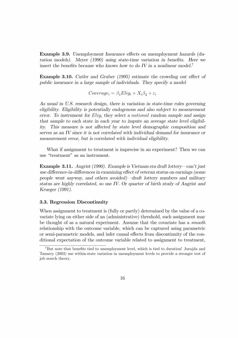
Example 3.9. Unemployment Insurance effects on unemployment hazards (du-ration models). Meyer (1990) using state-time variation in benefits. Here weinsert the benefits because who knows how to do IV in a nonlinear model.7

Example 3.10. Cutler and Gruber (1995) estimate the crowding out effect ofpublic insurance in a large sample of individuals. They specify a model

Coveragei = β1Eligi +Xiβ2 + εi

As usual in U.S. research design, there is variation in state-time rules governingeligibility. Eligibility is potentially endogenous and also subject to measurementerror. To instrument for Eligi they select a national random sample and assignthat sample to each state in each year to impute an average state level eligibil-ity. This measure is not affected by state level demographic composition andserves as an IV since it is not correlated with individual demand for insurance ormeasurement error, but is correlated with individual eligibility.

What if assignment to treatment is imprecise in an experiment? Then we canuse “treatment” as an instrument.

Example 3.11. Angrist (1990). Example is Vietnam era draft lottery–can’t justuse difference-in-differences in examining effect of veteran status on earnings (somepeople went anyway, and others avoided)–draft lottery numbers and militarystatus are highly correlated, so use IV. Or quarter of birth study of Angrist andKrueger (1991).

3.3. Regression Discontinuity

When assignment to treatment is (fully or partly) determined by the value of a co-variate lying on either side of an (administrative) threshold, such assignment maybe thought of as a natural experiment. Assume that the covariate has a smoothrelationship with the outcome variable, which can be captured using parametricor semi-parametric models, and infer causal effects from discontinuity of the con-ditional expectation of the outcome variable related to assignment to treatment,

7But note that benefits tied to unemployment level, which is tied to duration! Jurajda andTannery (2003) use within-state variation in unemployment levels to provide a stronger test ofjob search theory.

16

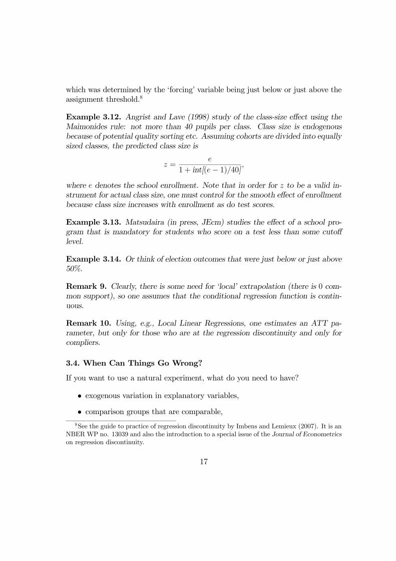
which was determined by the ‘forcing’ variable being just below or just above theassignment threshold.8

Example 3.12. Angrist and Lave (1998) study of the class-size effect using theMaimonides rule: not more than 40 pupils per class. Class size is endogenousbecause of potential quality sorting etc. Assuming cohorts are divided into equallysized classes, the predicted class size is

z =e

1 + int[(e− 1)/40] ,

where e denotes the school enrollment. Note that in order for z to be a valid in-strument for actual class size, one must control for the smooth effect of enrollmentbecause class size increases with enrollment as do test scores.

Example 3.13. Matsudaira (in press, JEcm) studies the effect of a school pro-gram that is mandatory for students who score on a test less than some cutofflevel.

Example 3.14. Or think of election outcomes that were just below or just above50%.

Remark 9. Clearly, there is some need for ‘local’ extrapolation (there is 0 com-mon support), so one assumes that the conditional regression function is contin-uous.

Remark 10. Using, e.g., Local Linear Regressions, one estimates an ATT pa-rameter, but only for those who are at the regression discontinuity and only forcompliers.

3.4. When Can Things Go Wrong?

If you want to use a natural experiment, what do you need to have?

• exogenous variation in explanatory variables,

• comparison groups that are comparable,8See the guide to practice of regression discontinuity by Imbens and Lemieux (2007). It is an

NBER WP no. 13039 and also the introduction to a special issue of the Journal of Econometricson regression discontinuity.

17

• explanatory variables that explain, and

• other explanations ruled out.

When can our quasi-experiments fail in delivering the right answer?

3.4.1. Internal Validity

Can the inference be made that the differences in the dependent variables werecaused by the differences in the relevant explanatory variables? Threats to internalvalidity:

1. Omitted variables–events other than the “experiment” that occur andmightprovide alternative explanations for the results.

2. Trends in outcomes–processes producing changes as a function of time perse, such as inflation, aging, and wage growth.

3. Misspecified variances–overstatement of the significance of statistical testsdue to effects such as the omission of group error terms that indicate matoutcomes for individual units are correlated.

4. Mismeasurement–changes in definitions or survey methods that producechanges in the measured variables (e.g. CPS unemployment and educationquestions), seam-bias problems (higher levels of changes reported for peri-ods between interviews than for analogous periods surveyed in the same in-terview), time-in-survey effects (rotation-group bias in CPS unemploymentrate).

5. Political economy–endogeneity of policy changes due to governmental re-sponses (e.g. state changes in policies as response to federal changes, or viceversa–see Besley and Case (NBER wp) or a crackdown on crime followinga few years of unusually high crime rates)

6. Simultaneity–endogeneity of explanatory variables due to joint determina-tion with outcomes.

7. Selection–assignment of observations to treatment groups in a manner thatleads to correlation between assignment and outcomes in the absence oftreatment (e.g. training literature: the “Ashenfelter dip”—decline in earnings

18

preceding program entry because people with recent labor market problemstend to be enrolled–hard to compare with nonparticipants)

8. Attrition–differential loss of respondents from treatment and comparisongroups (this is a problem even with randomized experiments–a good exam-ple is SIME/DIME negative income tax experiments).

9. Omitted interactions–differential trends in treatment and control groups, oromitted variables that change in different ways for treatments and controls.

Example 3.15. Return to Card’s Mariel Boatlift paper. In 1994 there was aboatlift that did not happen, but the unemployment rate for blacks in Miami roseby almost 4 percentage points between 1993 and 1995 (significant). See Angristand Krueger [HLE].

Example 3.16. Does Disability Insurance (DI) negatively affect labor force par-ticipation? Parsons (1980) suggests so (negative effect of replacement ratio =DI/wage). Bound (1989) says replacement ratio is a decreasing function of pastearnings and past earnings reflect pre-existing labor force participation patterns.So Bound estimates the effect of replacement ratio on workers who never appliedfor DI and gets the same negative effect. Next, he also studies those who appliedbut were turned down. These people are presumably healthier than the recipientsand they still did not work. So the effect is about being handicapped, not aboutcollecting DI.Similarly, test for the effect of the law before it took effect, for the effect of

marrying a highly-educated spouse before the marriage, for the effect of futureFDI on current growth of local companies etc.

3.4.2. External validity

Can the effects found be generalized? (This problem is not unique to naturalexperiments.) Threats to external validity:

1. Interaction of selection and treatment–treatment group not representativeof population.

2. Interaction of setting and treatment–effect of treatment different acrossgeographic or institutional settings.

3. Interaction of history and treatment–effect of treatment different acrosstime periods.

19

3.4.3. Possible Improvements

1. Multiple comparison groups: reduce the importance of randomness in asingle comparison group!

2. Multiple pre- or post- time periods (Seasonality. Do NJ and PA employmentlevels move together?)

3. Multiple treatment groups (high, medium, low wages prior to minimumwagehave different “treatments”)

4. Reversal of policy/treatment.

3.5. Testing Non-Experimental Methods

The way to test non-experimental estimation approaches is to compare their re-sults to those based on experiments.For example, consider measuring the effect of a training program. In Econo-

metrics IV we covered the Heckman’s λ approach to solving the selection on un-observables by exploiting an exclusion restriction.9 The method implicitly createsthe counterfactual. (Recall Section 3.1 for how the counterfactual is created in anexperiment.) LaLonde (1986) has experimental outcome and pretends that it’snot available, estimates the Heckman’s λ and finds it inaccurate.10

Similarly, Friedlander and Robins (1995) ask if one can use the cross-statecomparison groups typically invoked in panel data studies with state-level vari-ation in policies. They have experimental comparison groups from 4 states andconstruct non-experimental comparison groups (i) across-state, (ii) within-state,and (iii) before treatment. They also employ statistical tests based on the ideathat the program should have no effect before it is implemented and consider bothlong-run and short-run effects (because of, e.g., the Ashenfelter dip). They findthat the cross-state comparison fails miserably and that within-state fares betterbut is still noisy. The statistical tests do little to improve the results.

9That is: estimate one equation for who enters the program and another equation for theeffect of the program, controlling for the mean difference in the unobservables across participantsand the eligible non-participants.10See Heckman, LaLonde, and Smith (1998) “The Economics and Econometrics of Active

Labor Market Policies,” [HLE]

20

There are specific tests one should apply when using a regression discontinu-ity design. See the guide to practice of regression discontinuity by Imbens andLemieux (2007).

4. Defining Goals for Policy Analysis

Often we only want to understand certain phenomenon and we use IV to focuson a ‘clean’ sources of variation. However, in many cases we want to estimatethe effect of a particular policy/program. We need to clarify what kind of acounterfactual (“what if”) question we have in mind. For example when we wantto know about the effect of unions on wages, is the effect defined relative to a thecurrent level of unionization, a world where everybody is unionized, or a situationwhere there are no unions? We need to distinguish between the causal effect on anindividual in the current status quo and the comparison of different equilibriumsituations with no or full unionization. Typically, in most program evaluation weask only about partial equilibrium effects; no answers given on across-board policyevaluation (such as making every student go to college) — no general equilibriumeffects are usually taken into account.

Example 4.1. Knowledge Lift by Albrecht, van den Berg, Vroman: study theeffect of a very large skill upgrade programs in Sweden by first studying the effectof program participation on individual labor market outcomes. Second, theystudy the effect on labor market equilibrium. For the effects at the individuallevel, they apply fixed effect methods. For the equilibrium effects, they calibratean equilibrium search model.

The literature makes clear the key need to properly define the policy parametersof interest : What do we want to know? The effect of the program treatment onthe treated (TT; useful for cost-benefit analysis), the effect of the program onuntreated (whom we could make participate), the average treatment effect in thepopulation (ATE), or a treatment effect related to a specific new policy.See Econometrics IV for a comparison of the two methods we know for esti-

mating these parameters: (i) sample selection correction using a model of choicewith an excluded variable (IV) and (ii) direct regression estimation using IV from,e.g., a natural experiment. If the outcome is observed only under one choice, thensample selection is the only available approach, of course. We discuss the LATE

21

interpretation of IV in Econometrics IV.11

Example 4.2. Angrist and Krueger (1991) use quarter of birth and compulsoryschooling laws requiring children to enrol at age 6 and remain in school until their16th birthday to estimate returns to education. First, they show that there is arelationship between quarter of birth and educational attainment (Figure 1) sothat the estimated return is essentially a rescaled difference in average earningsby quarter of birth.12 Note that this approach uses only a small part of theoverall variation in schooling; in particular, the variation comes from those whoare unlikely to have higher education. (The IV appears valid precisely becausequarter of birth does not affect earnings and education of those with at leasta college degree, because these people are not constrained by the compulsoryschooling laws.)

(i) Having a natural experiment is wonderful in that we feel certain about theexogeneity of the IV. However, it may lead to estimates of the causal effect foronly the group affected by the experiment. Alternatively, if we have many IVs, wecan sketch the range of treatment effects. (ii) Parametric sample selection meth-ods may be sensitive to distributional assumptions, but recent semi-parametricextensions may allow for direct quantification of policy-relevant effects. (iii) Onemust be very careful when choosing non-experimental comparison groups in usualresearch designs; having more groups of different type and testing the differencesin the outcome is desirable.Some of the most interesting research today combines structural model estima-

tion, which allows for the generation of policy predictions, with exogenous (naturalexperiment) idenfitication. You either test your structure using the experimentor identify it using the experiment. See, e.g., papers by Atanassio, Meghir andothers or Wolpin and Todd and others on the Progressa experiment in Mexico.

11For an introduction to LATE, see <http://www.irs.princeton.edu/pubs/pdfs/415.pdf>.For an extensive set of presentation slides on the problem of causality and LATE IV see<http://www.iue.it/Personal/Ichino/air10.pdf>.12Look up Indirect Least Squares in Econometrics IV. Angrist and Krueger (1991) find that

men born in the first quarter (a) have about one-tenth of a year less schooling than men bornin later quarters, and (b) earn about 0.1 percent less. The ratio of the difference in earnings tothe difference in schooling, about 0.10 is an IV estimate.

22

5. Other Selected Methods

5.1. Oaxaca-Blinder Decompositions

Often, you want to use Least Squares regressions to explain (account) the sourcesof the difference in the outcomes across two groups of workers, countries, etc.(Think of regression as a conditional expectation.) For example, a vast and ul-timately unsuccessful literature aimed at measuring the extent of wage discrimi-nation has followed Oaxaca (1973) and Blinder (1973) in decomposing the overallmean wage difference between the advantaged (men) and disadvantaged (women)into two parts: the first reflecting the difference in average productive endow-ments of individuals in each group and the second part due to the differencesin coefficients. Following this approach, one first estimates logarithmic wage re-gressions separately for each gender, controlling for explanatory variables. Thedecomposition technique relies on the fact that the fitted regressions pass throughthe sample means13 as follows:

lnwg =cβg 0Xg, g ∈ f,m, (5.1)

where f denotes females and m denotes males, lnwg is the gender-specific meanof the natural logarithm of hourly wage, and where Xg represents the respectivevectors of mean values of explanatory variables for men and women. Finally, cβmand cβf are the corresponding vectors of estimated coefficients. A general form ofthe mean wage decomposition is as follows:

lnwm − lnwf = (Xm −Xf)0eβ + [Xm

0(cβm − eβ) +Xf

0(eβ −cβf)], (5.2)

where eβ represents a counter-factual non-discriminatory wage structure. The firstterm on the right hand side of equation 5.2 represents that part of the totallogarithmic wage difference which stems from the difference in average productivecharacteristics across gender. The second term originates in the differences ingender-specific coefficients from the non-discriminatory wage structure and is ofteninterpreted as reflecting wage discrimination.14

13This idea does not work in quantile regressions. See Machado and Mata for the methodapplicable in median regressions.14There have been objections to this decomposition approach. First, by focusing on the mean

gap, it ignores meaningful differences in gender-specific wage distributions. Second, if character-istics which might differ between males and females are omitted in the vector of regressors, thecontribution of these characteristics will be captured by the constant term and will erroneouslyappear in the measure of discrimination.

23

Remark 11. Using βmor βf for eβ corresponds to estimating the ATU or ATT,respectively (when being a female is the “treatment”.

Remark 12. Nopo (2004) and Black et al. (2005) and others now point out tomatching as a preferred alternative to parametric methods when support is notperfectly overlapping. For example, Jurajda and Paligorova (2006) compare wagesof female and male top managers.

There are a number of variants of this method depending on how one simu-lates the non-discriminatory wage structure eβ. Neumark (1988) and Oaxaca andRansom (1994) suggest the use of regression coefficients based on pooled dataincluding both men and women, arguing that they provide a good estimate ofa competitive non-discriminatory norm.15 Alternatively, one can use a similarapproximation based on weighting the male and female coefficients with sampleproportions of each sex (Macpherson and Hirsh, 1995).It is not always clear how you apply the method in non-linear models (see Ham

et al., 1998, AER). Recently, the decomposition has been extended to quantile(median) regressions by Machado and Mata (2000).16 There is a versions of thisdecomposition for Probit (Myeong-Su Yun, 2004). In a recent paper, he also addsstandard errors for this decomposition.17 Finally, there is an invariance problemthat has to do with the choice of the base category (affecting the constant andhence the unexplained part).There are important extensions taking the idea beyond first moments and

into decomposing whole distributions. See DiNardo, Fortin, and Lemiuex (1996,Econometrica) and Bourguignon, Ferreira, and Leite “Beyond Oaxaca-Blinder:Accounting for Differences in Household Income Distributions”. The DiNardo etal. decomposition has been programmed into Stata.

5.2. Meta Analysis

Very often, researchers explore a given question (in detail) using only one-countrydata. To follow up on the previous subsection, researchers often estimate theunexplained portion of the gender wage gap in one country. Next, the question is

15Neumark (1988) provides a theoretical justification for this approach using a model of dis-crimination with many types of labor where employers care about the proportion of women theyemploy.16See, e.g., Albrecht JOLE for an application of quantile regressions to gender wage gaps.17See also Fairlie (2005) Journal of Economic and Social Measurement.

24

how we cumulate knowledge across such studies. When you want to learn aboutthe impact of institutions or policies on the unexplained portion of the wage gapyou may collect data that consists of the estimates of other studies, which you thenregress on explanatory variables capturing the country-time specific variables.18

There is another potential use of Meta analysis: When scientists report theirresults, they are naturally driven to report important useful findings, that is thosethat reject the null hypothesis of no effect. One can analyze the set of existingresults to see if there is “reporting” “drawer” bias. That is, one can estimatea regression using the results from other studies, asking about the effect on thepublished results of the method of estimation used, type of data, etc. and thesize of the standard error. Consider for example the estimation of returns toeducation. IV studies typically have larger standard errors and typically reportlarger (significant) returns. See Ashenfelter, Harmon and Oosterbeek. “A Reviewof Estimates of the Schooling/Earnings Relationship, with Tests for PublicationBias.” Labour Economics (1999).19 If there is no bias in reporting, the estimatesshould not be correlated with their standard error. If, however, researchers aremore likely to report higher estimates when standard errors increase (IV), this willresult in sample selection (non-representative sample of all estimated results).

5.3. Expectations

See Manski (2004) “Measuring expectations,” Econometrica 72 (5): 1329-1376.

6. References

Abowd, John M. and Francis Kramarz. (1999) “The Analysis of Labor Markets Using Matched

Employer-Employee Data,” in Handbooks in Economics, vol. 5. Handbook of labor

economics. Volume 3B. Amsterdam; New York and Oxford: Elsevier Science, North-

Holland, 1999; pages 2629-2710

Acemoglu, Daron, David H. Autor and David Lyle. (2002) “Women, War and Wages: The

Effect of Female Labor Supply on the Wage Structure at Mid-Century,” NBER Working

Paper No. 9013.

18See work by Winter-Ebmer and others explaining the gender wage gap across countries. Itis important to know that there are a number of econometrics problems with this approach.19For another application of meta-analysis see Card and Krueger “Myth and Measurement”

book on minimum wages.

25

Angrist, Joshua D. (1990) “Lifetime Earnings and the Vietnam Era Draft Lottery: Evidence

from Social Security Administrative Records,” American Economic Review; 80(3), June

1990, pages 313-36.

Angrist, Joshua D. (1995) “The Economic Returns to Schooling in the West Bank and Gaza

Strip,” American Economic Review ; 85(5), December 1995, pages 1065-87.

Angrist Joshua, D. (1998) “Estimating the Labor Market Impact of Voluntary Military Service

Using Social Security Data on Military Applicants,” Econometrica; 66(2), March 1998,

pages 249-88.

Angrist, Joshua D. and Alan B. Krueger. (1991) “Does Compulsory School Attendance Affect

Schooling and Earnings?” Quarterly Journal of Economics; 106(4), November 1991, pages

979-1014.

Angrist Joshua D. and Alan B. Krueger. (1999) “Empirical Strategies in Labor Economics,”

in Handbooks in Economics, vol. 5. Handbook of Labor Economics. Volume 3A. Ams-

terdam; New York and Oxford: Elsevier Science, North-Holland, 1999, pages 1277-1366.

Angrist, Joshua D. and Alan B. Krueger. (2001) “Instrumental Variables and the Search for

Identification: From Supply and Demand to Natural Experiments,” Journal of Economic

Perspectives; 15(4), Fall 2001, pages 69-85.

Angrist, Joshua D. and Kevin Lang. (2002) “How Important are Classroom Peer Effects?

Evidence from Boston’s Metco Program,” NBER Working Paper No. 9263.

Ashenfelter, Orley and David Card. (1985) “Using the Longitudinal Structure of Earnings to

Estimate the Effect of Training Programs,” Review of Economics and Statistics; 67(4),

November 1985, pages 648-60.

Ashenfelter, Orley, Colm Harmon and Hessel Oosterbeek. (1999) “A Review of Estimates of the

Schooling/Earnings Relationship, with Tests for Publication Bias,” Labour Economics;

6(4), November 1999, pages 453-70.

Ashenfelter, Orley and Michael Greenstone. (2002) “Using Mandated Speed Limits to Measure

the Value of a Statistical Life,” NBER Working Paper No. 9094.

Attanasio, Orazio, Costas Meghir and Ana Santiago. (2001) “Education Choices in Mexico:

Using a Structural Model and Randomized Experiment to Evaluate Progress,” mimeo,

Intra American Development Bank.20

20http://www.iadb.org/res/files/ams1.pdf

26

Bell, B., Nickell, S. and G. Quintini (2002) “Wage equations, wage curves, and all that,”Labour

Economics, 9, 341-360.

Bertrand, Marianne, Esther Duflo and Sendhil Mullainathan. (2002) “How Much Should We

Trust Differences-in-Differences Estimates?” NBER Working Paper No. 8841.

Bertrand, Marianne and Sendhil Mullainathan. (2001) “Do People Mean What They Say?

Implications for Subjective Survey Data,” American Economic Review; 91(2), May 2001,

pages 67-72.

Besley, Timothy and Anne Case. (1995) “Unnatural Experiments? Estimating the Incidence of

Endogenous Policies,” Journal of Economic Perspectives; 9(2), Spring 1995, pages 3-22.

Bound, John. (1989) “The Health and Earnings of Rejected Disability Insurance Applicants,”

American Economic Review; 79(3), June 1989, pages 482-503.

Bound, John, David A. Jaeger and Regina M. Baker. (1995) “Problems with Instrumental

Variables Estimation When the Correlation between the Instruments and the Endogenous

Explanatory Variable Is Weak,” Journal of the American Statistical Association; 90(430),

June 1995, pages 443-50.

Bourguignon, Francois, Francisco H.G. Ferreira and Phillippe G. Leite. (2002) “Beyond Oax-

aca Blinder: Accounting for Differences in Household Income Distributions”, PUC-Rio,

mimeo.21

Card, David. (1990) “The Impact of the Mariel Boatlift on the Miami Labor Market,” Indus-

trial and Labor Relations Review; 43(2), January 1990, pages 245-57.

Card, David. (1992) “Using regional variation in wages to measure the effects of the federal

minimum wage,” Industrial and Labor Relations Review; 46(1), pages 22-37.

Card, David. (1993) “Using Geographic Variation in College Proximity to Estimate the Return

to Schooling,” NBER Working Paper No. 4483.

Card, David and Alan B. Krueger. (1994) “Minimum Wages and Employment: A Case Study

of the Fast-Food Industry in New Jersey and Pennsylvania,” American Economic Review;

84(4), September 1994, pages 772-93.

Card, David and Alen B. Krueger (1995) Myth and measurement: The new economics of the

minimum wage, Princeton: Princeton University Press, 1995.

21http://www.econ.puc-rio.br/PDF/td452.pdf

27

Carneiro, Pedro, James J. Heckman and Edward Vytlacil. (2001) “Estimating the Return to

Education When it Varies Among Individuals,” mimeo, University of Chicago, 2001.22

Cutler, David M. and Jonathan Gruber. (1996) “Does Public Insurance Crowd Out Private

Insurance?” The Quarterly Journal of Economics; 111 (2), May 1996, pages 391-430.

Deaton, Angus. (1985) “Panel Data from Time Series of Cross-Sections,” Journal of Econo-

metrics; 30(1 2), Oct.-Nov. 1985, pages 109-26.

Deaton, Angus.(1997) “The analysis of household surveys: A microeconometric approach to

development policy, Baltimore and London,” Johns Hopkins University Press for the

World Bank, 1997, pp: 67-72.

DiNardo, John, Nicole M. Fortin and Thomas Lemieux. (1996) “Labor Market Institutions

and the Distribution of Wages, 1973-1992: A Semiparametric Approach,” Econometrica;

64(5), September 1996, pages 1001-44.

Durlauf, Steven, N. (2002) “On the Empirics of Social Capital,” Economic Journal 112, F459-

479.

Friedlander, Daniel and Philip K. Robins. (1995) “Evaluating Program Evaluations: New

Evidence on Commonly Used Nonexperimental Methods,” American Economic Review;

85(4), September 1995, pages 923-37.

Freeman, Richard, B. (1998) “War of the models: Which labour market institutions for the

21st century?”Labour Economics 5, pp. 1-24.

Gould, Eric D. and M. Daniel Paserman. (2003) “Waiting for Mr. Right: Rising Inequality

and Declining Marriage Rates” Journal of Urban Economics, forthcoming, 2003.

Griliches, Zvi. (1977) “Estimating the Returns to Schooling: Some Econometric Problems,”

Econometrica, 45(1), Jan. 1977, pages 1-22.

Gruber, Jonathan. (1994) “The Incidence of Mandated Maternity Benefits,” American Eco-

nomic Review; 84(3), June 1994, pages 622-41.

Haavelmo, Trygve. (1944) “The Probability Approach in Econometrics,” Econometrica; 12,

July 1944, pages 1-118.

22http://lily.src.uchicago.edu/~dvmaster/FILES/estimating_complete.pdf

28

Ham, John C. and Robert J. LaLonde. (1996) “The Effect of Sample Selection and Initial

Conditions in Duration Models: Evidence from Experimental Data on Training,” Econo-

metrica; 64(1), January 1996, pages 175-205.

Ham, John C., Jan Svejnar and Katherine Terrell. (1998) “Unemployment and the Social

Safety Net during Transitions to a Market Economy: Evidence from the Czech and

Slovak Republics,” American Economic Review; 88(5), December 1998, pages 1117-42.

Heckman, James J. (1974) “Shadow Prices, Market Wages, and Labor Supply,” Econometrica;

42(4), July 1974, pages 679-94.

Heckman James J. (1979) “Sample Selection Bias as a Specification Error,” Econometrica;

47(1), January 1979, pages 153-161.

Heckman, James J. (2000) “Causal Parameters and Policy Analysis in Economics: A Twentieth

Century Retrospective,” Quarterly Journal of Economics; 115(1), February 2000, pages

45-97.

Heckman, James J., Robert J. Lalonde and Jeffrey A. Smith. (1999) “The Economics and

Econometrics of Active Labor Market Programs,” in Handbooks in Economics, vol. 5.

Handbook of labor economics. Volume 3A, Amsterdam; New York and Oxford: Elsevier

Science, North-Holland, 1999, pages 1865-2097.

Heckman, James and Edward Vytlacil. (1998) “Instrumental Variables Methods for the Cor-

related Random Coefficient Model: Estimating the Average Rate of Return to Schooling

When the Return Is Correlated with Schooling,” Journal of Human Resources; 33(4), Fall

1998, pages 974-87.

Hogan, Vincent and Roberto Rigobon. (2002) “Using Heteroscedasticity to Estimate the Re-

turns to Education,” NBER Working Paper No. 9145.

Jurajda, Stepan. (2003) “Gender Wage Gap and Segregation in Late Transition,” Journal of

Comparative Economics, forthcoming, September 2003.

Jurajda, Stepan and Frederick J. Tannery. (2003) “Unemployment Spells and the Extended

Unemployment Benefits in Local Labor Markets,” Industrial and Labor Relations Review,

forthcoming, 2003.

LaLonde, Robert J. (1986) “Evaluating the Econometric Evaluations of Training Programs

with Experimental Data,” American Economic Review; 76(4), September 1986, pages

604-20.

29

Leamer, Edward E. (1978) “Regression Selection Strategies and Revealed Priors,” Journal of

the American Statistical Association; 73(363), September 1978, pages 580-87.

Machin, Stephen, Alan Manning and Lupin Rahman. (2001) “The Economic Effects of the

Introduction of the UK National Minimum Wage.”23

Macpherson, David A. and Barry T. Hirsch. (1995) “Wages and Gender Composition: Why Do

Women’s Jobs Pay Less?” Journal of Labor Economics; 13(3), July 1995, pages 426-71.

Madrian, Brigitte C. (1993) “Employment-Based Health Insurance and Job Mobility: Is There

Evidence of Job-Lock?” NBER Working Paper No. 4476.

Manski, Charles F. (1995) Identification problems in the social sciences, Cambridge and Lon-

don: Harvard University Press, 1995.

Marschak, Jacob. (1953) “Economic Measurements For Policy and Prediction,” in Studies in

Econometric Methods, ed. by W. Hood and T. Koopmans, New York: John Wiley, pages

1-26.

Meyer, Bruce D. (1990) “Unemployment Insurance and Unemployment Spells,” Econometrica;

58(4), July 1990, pages 757-82.

Meyer, Bruce D. (1995) “Natural and Quasi-experiments in Economics,” Journal of Business

and Economic Statistics; 13(2), April 1995, 151-61.

Meyer, Bruce D., Kip W. Viscusi and David L. Durbin. (1995) “Workers’ Compensation and

Injury Duration: Evidence from a Natural Experiment,” American Economic Review;

85(3), June 1995, pages 322-40.

Neumark, David. (1988) “Employers’ Discriminatory Behavior and the Estimation of Wage

Discrimination,” Journal of Human Resources; 23(3), Summer 1988, pages 279-95.

Oaxaca, Ronald. (1973) “Male-Female Wage Differentials in Urban Labor Markets,” Interna-

tional Economic Review; 14(3), Oct. 1973, pages 693-709.

Oaxaca, Ronald L. and Michael R. Ransom. (1994) “On Discrimination and the Decomposition

of Wage Differentials,” Journal of Econometrics; 61(1), March 1994, pages 5-21.

Parsons, Donald O. (1980) “The Decline in Male Labor Force Participation,” Journal of Polit-

ical Economy ; 88(1), Feb. 1980, pages 117-34.

23http://www.cerge.cuni.cz/pdf/events/papers/010312_t.pdf

30

Popper, Karl R. (1959) The Logic of Scientific Discovery, London: Hutchinson.

Roy, Andrew D. (1951) “Some Thoughts on the Distribution of Earnings,” Oxford Economic

Papers; 3, June 1951, pages 135-46.

Todd, Petra and Kenneth I. Wolpin. (2002) “Using Experimental Data to Validate a Dynamic

Behavioral Model of Child Schooling and Fertility.”24

Willis, Robert J. and Sherwin Rosen. (1979) “Education and Self-Selection,” Journal of Polit-

ical Economy ; 87(5), Oct. 1979, pages 7-36.

24http://athena.sas.upenn.edu/~petra/progresa4.pdf

31