Embed Size (px)
Citation preview
Lecture Notes on
GRAPH THEORY
Tero HarjuDepartment of Mathematics
University of TurkuFIN-20014 Turku, Finland
1994 – 2012
Contents
1 Introduction . . . . . . . . . . . . . . . . . . . . . . . . . . . . . . . . . . . . . . . . . . . . . . . . . . . . . . . . . . . . . . . . . . . . 21.1 Graphs and their plane figures . . . . . . . . . . . . . . . . . . . . . . . . . . . . . . . . . . . . . . . . . . . . . . . 41.2 Subgraphs . . . . . . . . . . . . . . . . . . . . . . . . . . . . . . . . . . . . . . . . . . . . . . . . . . . . . . . . . . . . . . . . . . 71.3 Paths and cycles . . . . . . . . . . . . . . . . . . . . . . . . . . . . . . . . . . . . . . . . . . . . . . . . . . . . . . . . . . . . . 11
2 Connectivity of Graphs . . . . . . . . . . . . . . . . . . . . . . . . . . . . . . . . . . . . . . . . . . . . . . . . . . . . . . . . . . 162.1 Bipartite graphs and trees. . . . . . . . . . . . . . . . . . . . . . . . . . . . . . . . . . . . . . . . . . . . . . . . . . . . 162.2 Connectivity . . . . . . . . . . . . . . . . . . . . . . . . . . . . . . . . . . . . . . . . . . . . . . . . . . . . . . . . . . . . . . . . 23
3 Tours and Matchings . . . . . . . . . . . . . . . . . . . . . . . . . . . . . . . . . . . . . . . . . . . . . . . . . . . . . . . . . . . . 293.1 Eulerian graphs . . . . . . . . . . . . . . . . . . . . . . . . . . . . . . . . . . . . . . . . . . . . . . . . . . . . . . . . . . . . . 293.2 Hamiltonian graphs . . . . . . . . . . . . . . . . . . . . . . . . . . . . . . . . . . . . . . . . . . . . . . . . . . . . . . . . . 313.3 Matchings . . . . . . . . . . . . . . . . . . . . . . . . . . . . . . . . . . . . . . . . . . . . . . . . . . . . . . . . . . . . . . . . . . 35
4 Colourings . . . . . . . . . . . . . . . . . . . . . . . . . . . . . . . . . . . . . . . . . . . . . . . . . . . . . . . . . . . . . . . . . . . . . . 424.1 Edge colourings . . . . . . . . . . . . . . . . . . . . . . . . . . . . . . . . . . . . . . . . . . . . . . . . . . . . . . . . . . . . . 424.2 Ramsey Theory . . . . . . . . . . . . . . . . . . . . . . . . . . . . . . . . . . . . . . . . . . . . . . . . . . . . . . . . . . . . . 464.3 Vertex colourings . . . . . . . . . . . . . . . . . . . . . . . . . . . . . . . . . . . . . . . . . . . . . . . . . . . . . . . . . . . . 52
5 Graphs on Surfaces . . . . . . . . . . . . . . . . . . . . . . . . . . . . . . . . . . . . . . . . . . . . . . . . . . . . . . . . . . . . . 605.1 Planar graphs . . . . . . . . . . . . . . . . . . . . . . . . . . . . . . . . . . . . . . . . . . . . . . . . . . . . . . . . . . . . . . . 605.2 Colouring planar graphs . . . . . . . . . . . . . . . . . . . . . . . . . . . . . . . . . . . . . . . . . . . . . . . . . . . . . 675.3 Genus of a graph . . . . . . . . . . . . . . . . . . . . . . . . . . . . . . . . . . . . . . . . . . . . . . . . . . . . . . . . . . . . 74
6 Directed Graphs . . . . . . . . . . . . . . . . . . . . . . . . . . . . . . . . . . . . . . . . . . . . . . . . . . . . . . . . . . . . . . . . 826.1 Digraphs . . . . . . . . . . . . . . . . . . . . . . . . . . . . . . . . . . . . . . . . . . . . . . . . . . . . . . . . . . . . . . . . . . . 826.2 Network Flows . . . . . . . . . . . . . . . . . . . . . . . . . . . . . . . . . . . . . . . . . . . . . . . . . . . . . . . . . . . . . . 88
Index . . . . . . . . . . . . . . . . . . . . . . . . . . . . . . . . . . . . . . . . . . . . . . . . . . . . . . . . . . . . . . . . . . . . . . . . . . . . . . . 95
1
Introduction
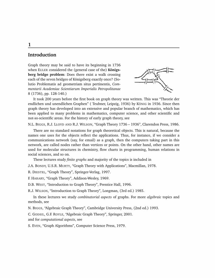
Graph theory may be said to have its beginning in 1736when EULER considered the (general case of the) Königs-berg bridge problem: Does there exist a walk crossingeach of the seven bridges of Königsberg exactly once? (So-lutio Problematis ad geometriam situs pertinentis, Com-
mentarii Academiae Scientiarum Imperialis Petropolitanae
8 (1736), pp. 128-140.)
It took 200 years before the first book on graph theory was written. This was “Theorie derendlichen und unendlichen Graphen” ( Teubner, Leipzig, 1936) by KÖNIG in 1936. Since thengraph theory has developed into an extensive and popular branch of mathematics, which hasbeen applied to many problems in mathematics, computer science, and other scientific andnot-so-scientific areas. For the history of early graph theory, see
N.L. BIGGS, R.J. LLOYD AND R.J. WILSON, “Graph Theory 1736 – 1936”, Clarendon Press, 1986.
There are no standard notations for graph theoretical objects. This is natural, because thenames one uses for the objects reflect the applications. Thus, for instance, if we consider acommunications network (say, for email) as a graph, then the computers taking part in thisnetwork, are called nodes rather than vertices or points. On the other hand, other names areused for molecular structures in chemistry, flow charts in programming, human relations insocial sciences, and so on.
These lectures study finite graphs and majority of the topics is included in
J.A. BONDY, U.S.R. MURTY, “Graph Theory with Applications”, Macmillan, 1978.
R. DIESTEL, “Graph Theory”, Springer-Verlag, 1997.
F. HARARY, “Graph Theory”, Addison-Wesley, 1969.
D.B. WEST, “Introduction to Graph Theory”, Prentice Hall, 1996.
R.J. WILSON, “Introduction to Graph Theory”, Longman, (3rd ed.) 1985.
In these lectures we study combinatorial aspects of graphs. For more algebraic topics andmethods, see
N. BIGGS, “Algebraic Graph Theory”, Cambridge University Press, (2nd ed.) 1993.
C. GODSIL, G.F. ROYLE, “Algebraic Graph Theory”, Springer, 2001.and for computational aspects, see
S. EVEN, “Graph Algorithms”, Computer Science Press, 1979.
3
In these lecture notes we mention several open problems that have gained respect amongthe researchers. Indeed, graph theory has the advantage that it contains easily formulated openproblems that can be stated early in the theory. Finding a solution to any one of these problemsis another matter.
Sections with a star (∗) in their heading are optional.
Notations and notions
• For a finite set X , |X | denotes its size (cardinality, the number of its elements).• Let
[1, n] = {1,2, . . . , n},
and in general,[i, n] = {i, i + 1, . . . , n}
for integers i ≤ n.• For a real number x , the floor and the ceiling of x are the integers
⌊x⌋=max{k ∈ Z | k ≤ x} and ⌈x⌉=min{k ∈ Z | x ≤ k}.
• A family {X1, X2, . . . , Xk} of subsets X i ⊆ X of a set X is a partition of X , if
X =⋃
i∈[1,k]
X i and X i ∩ X j = ; for all different i and j .
• For two sets X and Y ,X × Y = {(x , y) | x ∈ X , y ∈ Y }
is their Cartesian product, and
X△Y = (X \ Y )∪ (Y \ X )
is their symmetric difference. Here X \ Y = {x | x ∈ X , x /∈ Y }.• Two integers n, k ∈ N (often n = |X | and k = |Y | for sets X and Y ) have the same parity, ifboth are even, or both are odd, that is, if n≡ k (mod 2). Otherwise, they have opposite parity.
Graph theory has abundant examples of N P-complete problems. Intuitively, a problem isin P1 if there is an efficient (practical) algorithm to find a solution to it. On the other hand,a problem is in N P2, if it is first efficient to guess a solution and then efficient to check thatthis solution is correct. It is conjectured (and not known) that P 6= N P. This is one of the greatproblems in modern mathematics and theoretical computer science. If the guessing part in N P-problems can be replaced by an efficient systematic search for a solution, then P = N P. For anyone N P-complete problem, if it is in P, then necessarily P = N P.
1 Solvable – by an algorithm – in polynomially many steps on the size of the problem instances.2 Solvable nondeterministically in polynomially many steps on the size of the problem instances.
1.1 Graphs and their plane figures 4
1.1 Graphs and their plane figures
Let V be a finite set, and denote by
E(V ) = {{u, v} | u, v ∈ V, u 6= v} .
the 2-sets of V , i.e., subsets of two distinct elements.
DEFINITION. A pair G = (V, E) with E ⊆ E(V ) is called a graph (on V ). The elements of V arethe vertices of G, and those of E the edges of G. The vertex set of a graph G is denoted by VG
and its edge set by EG. Therefore G = (VG , EG).
In literature, graphs are also called simple graphs; vertices are called nodes or points; edgesare called lines or links. The list of alternatives is long (but still finite).
A pair {u, v} is usually written simply as uv. Notice that then uv = vu. In order to simplifynotations, we also write v ∈ G and e ∈ G instead of v ∈ VG and e ∈ EG .
DEFINITION. For a graph G, we denote
νG = |VG | and ǫG = |EG| .
The number νG of the vertices is called the order of G, and ǫG is the size of G. For an edgee = uv ∈ G, the vertices u and v are its ends. Vertices u and v are adjacent or neighbours, ifuv ∈ G. Two edges e1 = uv and e2 = uw having a common end, are adjacent with each other.
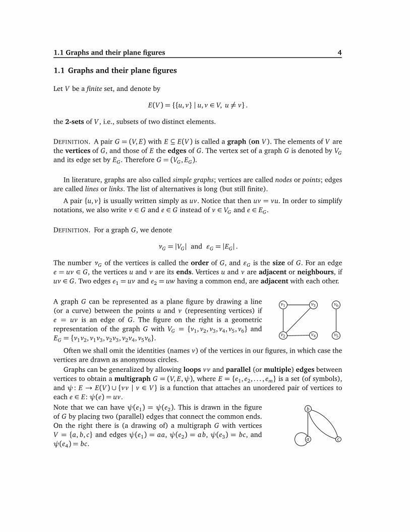
A graph G can be represented as a plane figure by drawing a line(or a curve) between the points u and v (representing vertices) ife = uv is an edge of G. The figure on the right is a geometricrepresentation of the graph G with VG = {v1, v2, v3, v4, v5, v6} andEG = {v1v2, v1v3, v2v3, v2v4, v5v6}.
v1
v2
v3
v4 v5
v6
Often we shall omit the identities (names v) of the vertices in our figures, in which case thevertices are drawn as anonymous circles.
Graphs can be generalized by allowing loops vv and parallel (or multiple) edges betweenvertices to obtain a multigraph G = (V, E,ψ), where E = {e1, e2, . . . , em} is a set (of symbols),and ψ: E → E(V ) ∪ {vv | v ∈ V} is a function that attaches an unordered pair of vertices toeach e ∈ E: ψ(e) = uv.
Note that we can have ψ(e1) = ψ(e2). This is drawn in the figureof G by placing two (parallel) edges that connect the common ends.On the right there is (a drawing of) a multigraph G with verticesV = {a, b, c} and edges ψ(e1) = aa, ψ(e2) = ab, ψ(e3) = bc, andψ(e4) = bc.
a
b
c
1.1 Graphs and their plane figures 5
Later we concentrate on (simple) graphs.
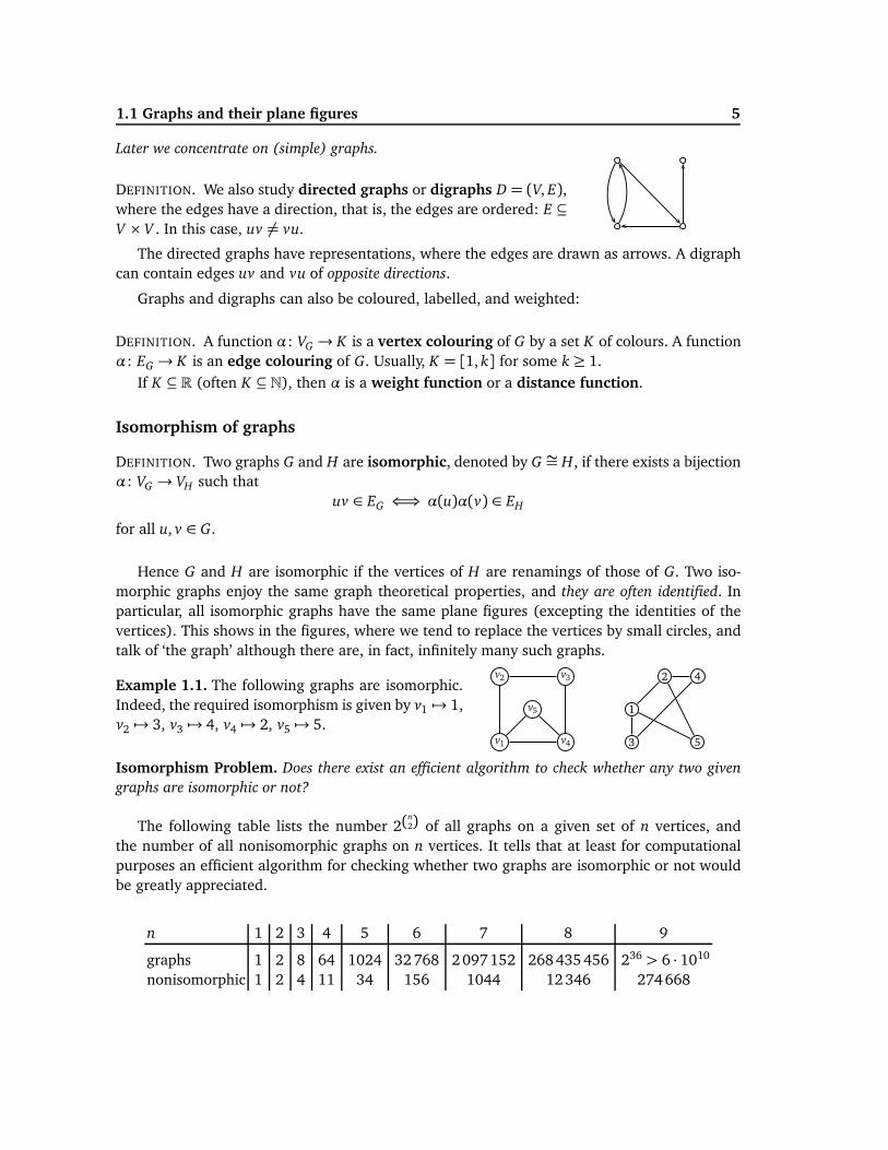
DEFINITION. We also study directed graphs or digraphs D = (V, E),where the edges have a direction, that is, the edges are ordered: E ⊆
V × V . In this case, uv 6= vu.
The directed graphs have representations, where the edges are drawn as arrows. A digraphcan contain edges uv and vu of opposite directions.
Graphs and digraphs can also be coloured, labelled, and weighted:
DEFINITION. A function α: VG → K is a vertex colouring of G by a set K of colours. A functionα: EG → K is an edge colouring of G. Usually, K = [1, k] for some k ≥ 1.
If K ⊆ R (often K ⊆ N), then α is a weight function or a distance function.
Isomorphism of graphs
DEFINITION. Two graphs G and H are isomorphic, denoted by G ∼= H, if there exists a bijectionα: VG → VH such that
uv ∈ EG ⇐⇒ α(u)α(v) ∈ EH
for all u, v ∈ G.
Hence G and H are isomorphic if the vertices of H are renamings of those of G. Two iso-morphic graphs enjoy the same graph theoretical properties, and they are often identified. Inparticular, all isomorphic graphs have the same plane figures (excepting the identities of thevertices). This shows in the figures, where we tend to replace the vertices by small circles, andtalk of ‘the graph’ although there are, in fact, infinitely many such graphs.
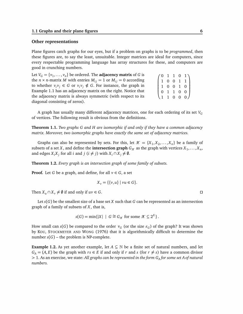
Example 1.1. The following graphs are isomorphic.Indeed, the required isomorphism is given by v1 7→ 1,v2 7→ 3, v3 7→ 4, v4 7→ 2, v5 7→ 5.
v1
v2 v3
v4
v5 1
3
42
5
Isomorphism Problem. Does there exist an efficient algorithm to check whether any two given
graphs are isomorphic or not?
The following table lists the number 2(n2) of all graphs on a given set of n vertices, and
the number of all nonisomorphic graphs on n vertices. It tells that at least for computationalpurposes an efficient algorithm for checking whether two graphs are isomorphic or not wouldbe greatly appreciated.
n 1 2 3 4 5 6 7 8 9
graphs 1 2 8 64 1024 32 768 2 097 152 268 435 456 236 > 6 · 1010
nonisomorphic 1 2 4 11 34 156 1044 12 346 274 668
1.1 Graphs and their plane figures 6
Other representations
Plane figures catch graphs for our eyes, but if a problem on graphs is to be programmed, thenthese figures are, to say the least, unsuitable. Integer matrices are ideal for computers, sinceevery respectable programming language has array structures for these, and computers aregood in crunching numbers.
Let VG = {v1, . . . , vn} be ordered. The adjacency matrix of G isthe n× n-matrix M with entries Mi j = 1 or Mi j = 0 accordingto whether vi v j ∈ G or vi v j /∈ G. For instance, the graph inExample 1.1 has an adjacency matrix on the right. Notice thatthe adjacency matrix is always symmetric (with respect to itsdiagonal consisting of zeros).
0 1 1 0 11 0 0 1 11 0 0 1 00 1 1 0 01 1 0 0 0
A graph has usually many different adjacency matrices, one for each ordering of its set VG
of vertices. The following result is obvious from the definitions.
Theorem 1.1. Two graphs G and H are isomorphic if and only if they have a common adjacency
matrix. Moreover, two isomorphic graphs have exactly the same set of adjacency matrices.
Graphs can also be represented by sets. For this, let X = {X1, X2, . . . , Xn} be a family ofsubsets of a set X , and define the intersection graph GX as the graph with vertices X1, . . . , Xn,and edges X iX j for all i and j (i 6= j) with X i ∩ X j 6= ;.
Theorem 1.2. Every graph is an intersection graph of some family of subsets.
Proof. Let G be a graph, and define, for all v ∈ G, a set
X v = {{v,u} | vu ∈ G}.
Then Xu ∩ X v 6= ; if and only if uv ∈ G. ⊓⊔
Let s(G) be the smallest size of a base set X such that G can be represented as an intersectiongraph of a family of subsets of X , that is,
s(G) =min{|X | | G ∼= GX for some X ⊆ 2X } .
How small can s(G) be compared to the order νG (or the size ǫG) of the graph? It was shownby KOU, STOCKMEYER AND WONG (1976) that it is algorithmically difficult to determine thenumber s(G) – the problem is NP-complete.
Example 1.2. As yet another example, let A ⊆ N be a finite set of natural numbers, and letGA = (A, E) be the graph with rs ∈ E if and only if r and s (for r 6= s) have a common divisor> 1. As an exercise, we state: All graphs can be represented in the form GA for some set A of natural
numbers.
1.2 Subgraphs 7
1.2 Subgraphs
Ideally, given a nice problem the local properties of a graph determine a solution. In thesesituations we deal with (small) parts of the graph (subgraphs), and a solution can be found tothe problem by combining the information determined by the parts. For instance, as we shalllater see, the existence of an Euler tour is very local, it depends only on the number of theneighbours of the vertices.
Degrees of vertices
DEFINITION. Let v ∈ G be a vertex a graph G. The neighbourhood of v is the set
NG(v) = {u ∈ G | vu ∈ G} .
The degree of v is the number of its neighbours:
dG(v) = |NG(v)| .
If dG(v) = 0, then v is said to be isolated in G, and if dG(v) = 1, then v is a leaf of the graph.The minimum degree and the maximum degree of G are defined as
δ(G) =min{dG(v) | v ∈ G} and ∆(G) =max{dG(v) | v ∈ G} .
The following lemma, due to EULER (1736), tells that if several people shake hands, thenthe number of hands shaken is even.
Lemma 1.1 (Handshaking lemma). For each graph G,
∑
v∈G
dG(v) = 2 · ǫG .
Moreover, the number of vertices of odd degree is even.
Proof. Every edge e ∈ EG has two ends. The second claim follows immediately from the firstone. ⊓⊔
Lemma 1.1 holds equally well for multigraphs, when dG(v) is defined as the number of edgesthat have v as an end, and when each loop vv is counted twice.
Note that the degrees of a graph G do not determine G. Indeed, there are graphs G = (V, EG)
and H = (V, EH ) on the same set of vertices that are not isomorphic, but for which dG(v) = dH(v)
for all v ∈ V .
1.2 Subgraphs 8
Subgraphs
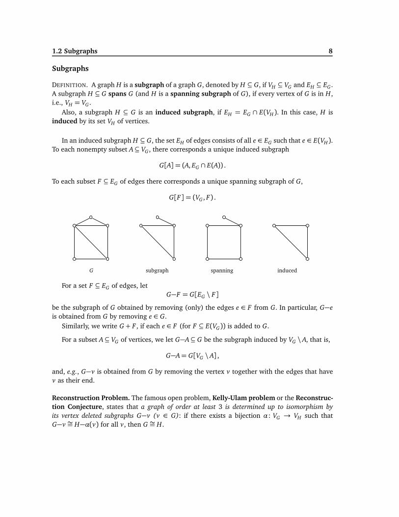
DEFINITION. A graph H is a subgraph of a graph G, denoted by H ⊆ G, if VH ⊆ VG and EH ⊆ EG .A subgraph H ⊆ G spans G (and H is a spanning subgraph of G), if every vertex of G is in H,i.e., VH = VG .
Also, a subgraph H ⊆ G is an induced subgraph, if EH = EG ∩ E(VH ). In this case, H isinduced by its set VH of vertices.
In an induced subgraph H ⊆ G, the set EH of edges consists of all e ∈ EG such that e ∈ E(VH).To each nonempty subset A⊆ VG , there corresponds a unique induced subgraph
G[A] = (A, EG ∩ E(A)) .
To each subset F ⊆ EG of edges there corresponds a unique spanning subgraph of G,
G[F] = (VG , F) .
G subgraph spanning induced
For a set F ⊆ EG of edges, letG−F = G[EG \ F]
be the subgraph of G obtained by removing (only) the edges e ∈ F from G. In particular, G−e
is obtained from G by removing e ∈ G.Similarly, we write G + F , if each e ∈ F (for F ⊆ E(VG)) is added to G.
For a subset A⊆ VG of vertices, we let G−A⊆ G be the subgraph induced by VG \ A, that is,
G−A= G[VG \ A] ,
and, e.g., G−v is obtained from G by removing the vertex v together with the edges that havev as their end.
Reconstruction Problem. The famous open problem, Kelly-Ulam problem or the Reconstruc-tion Conjecture, states that a graph of order at least 3 is determined up to isomorphism by
its vertex deleted subgraphs G−v (v ∈ G): if there exists a bijection α: VG → VH such thatG−v ∼= H−α(v) for all v, then G ∼= H.
1.2 Subgraphs 9
2-switches
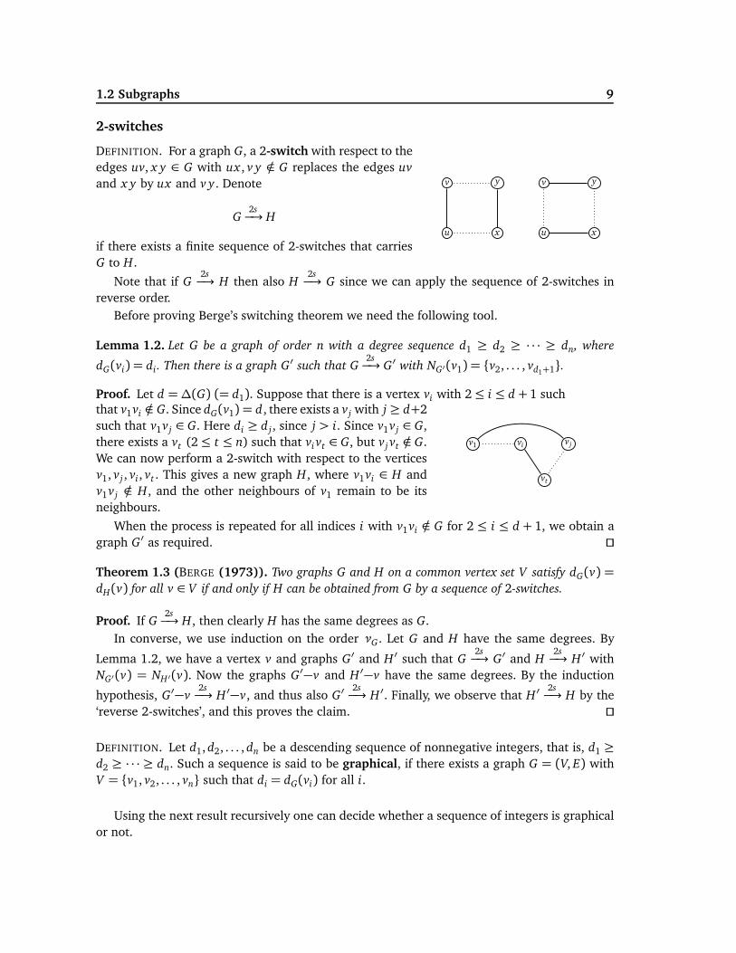
DEFINITION. For a graph G, a 2-switch with respect to theedges uv, x y ∈ G with ux , v y /∈ G replaces the edges uv
and x y by ux and v y. Denote
G2s−→ H
if there exists a finite sequence of 2-switches that carriesG to H.
u
v
x
y
u
v
x
y
Note that if G2s−→ H then also H
2s−→ G since we can apply the sequence of 2-switches in
reverse order.Before proving Berge’s switching theorem we need the following tool.
Lemma 1.2. Let G be a graph of order n with a degree sequence d1 ≥ d2 ≥ · · · ≥ dn, where
dG(vi) = di. Then there is a graph G′ such that G2s−→ G′ with NG′(v1) = {v2, . . . , vd1+1}.
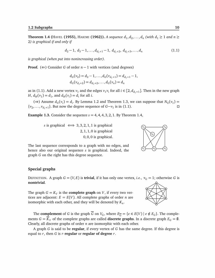
Proof. Let d =∆(G) (= d1). Suppose that there is a vertex vi with 2≤ i ≤ d + 1 suchthat v1vi /∈ G. Since dG(v1) = d , there exists a v j with j ≥ d+2such that v1v j ∈ G. Here di ≥ d j, since j > i. Since v1v j ∈ G,there exists a vt (2≤ t ≤ n) such that vi vt ∈ G, but v j vt /∈ G.We can now perform a 2-switch with respect to the verticesv1, v j , vi, vt . This gives a new graph H, where v1vi ∈ H andv1v j /∈ H, and the other neighbours of v1 remain to be itsneighbours.
v1 vi v j
vt
When the process is repeated for all indices i with v1vi /∈ G for 2 ≤ i ≤ d + 1, we obtain agraph G′ as required. ⊓⊔
Theorem 1.3 (BERGE (1973)). Two graphs G and H on a common vertex set V satisfy dG(v) =
dH(v) for all v ∈ V if and only if H can be obtained from G by a sequence of 2-switches.
Proof. If G2s−→ H, then clearly H has the same degrees as G.
In converse, we use induction on the order νG . Let G and H have the same degrees. By
Lemma 1.2, we have a vertex v and graphs G′ and H ′ such that G2s−→ G′ and H
2s−→ H ′ with
NG′(v) = NH′(v). Now the graphs G′−v and H ′−v have the same degrees. By the induction
hypothesis, G′−v2s−→ H ′−v, and thus also G′
2s−→ H ′. Finally, we observe that H ′
2s−→ H by the
‘reverse 2-switches’, and this proves the claim. ⊓⊔
DEFINITION. Let d1, d2, . . . , dn be a descending sequence of nonnegative integers, that is, d1 ≥
d2 ≥ · · · ≥ dn. Such a sequence is said to be graphical, if there exists a graph G = (V, E) withV = {v1, v2, . . . , vn} such that di = dG(vi) for all i.
Using the next result recursively one can decide whether a sequence of integers is graphicalor not.
1.2 Subgraphs 10
Theorem 1.4 (HAVEL (1955), HAKIMI (1962)). A sequence d1, d2, . . . , dn (with d1 ≥ 1 and n ≥
2) is graphical if and only if
d2 − 1, d3 − 1, . . . , dd1+1 − 1, dd1+2, dd1+3, . . . , dn (1.1)
is graphical (when put into nonincreasing order).
Proof. (⇐) Consider G of order n− 1 with vertices (and degrees)
dG(v2) = d2 − 1, . . . , dG(vd1+1) = dd1+1 − 1,
dG(vd1+2) = dd1+2, . . . , dG(vn) = dn
as in (1.1). Add a new vertex v1 and the edges v1vi for all i ∈ [2, dd1+1]. Then in the new graphH, dH(v1) = d1, and dH(vi) = di for all i.
(⇒) Assume dG(vi) = di. By Lemma 1.2 and Theorem 1.3, we can suppose that NG(v1) =
{v2, . . . , vd1+1}. But now the degree sequence of G−v1 is in (1.1). ⊓⊔
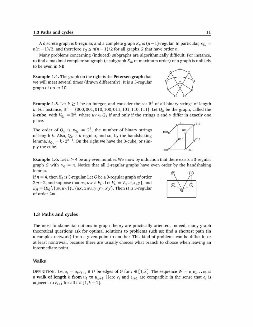
Example 1.3. Consider the sequence s = 4,4,4,3,2,1. By Theorem 1.4,
s is graphical ⇐⇒ 3,3,2,1,1 is graphical
2,1,1,0 is graphical
0,0,0 is graphical.
The last sequence corresponds to a graph with no edges, andhence also our original sequence s is graphical. Indeed, thegraph G on the right has this degree sequence.
v1
v2
v3
v4
v5
v6
Special graphs
DEFINITION. A graph G = (V, E) is trivial, if it has only one vertex, i.e., νG = 1; otherwise G isnontrivial.
The graph G = KV is the complete graph on V , if every two ver-tices are adjacent: E = E(V ). All complete graphs of order n areisomorphic with each other, and they will be denoted by Kn.
The complement of G is the graph G on VG , where EG = {e ∈ E(V ) | e /∈ EG}. The comple-ments G = KV of the complete graphs are called discrete graphs. In a discrete graph EG = ;.Clearly, all discrete graphs of order n are isomorphic with each other.
A graph G is said to be regular, if every vertex of G has the same degree. If this degree isequal to r, then G is r-regular or regular of degree r.
1.3 Paths and cycles 11
A discrete graph is 0-regular, and a complete graph Kn is (n−1)-regular. In particular, ǫKn=
n(n− 1)/2, and therefore ǫG ≤ n(n− 1)/2 for all graphs G that have order n.Many problems concerning (induced) subgraphs are algorithmically difficult. For instance,
to find a maximal complete subgraph (a subgraph Km of maximum order) of a graph is unlikelyto be even in NP.
Example 1.4. The graph on the right is the Petersen graph thatwe will meet several times (drawn differently). It is a 3-regulargraph of order 10.
Example 1.5. Let k ≥ 1 be an integer, and consider the set Bk of all binary strings of lengthk. For instance, B3 = {000,001,010,100,011,101,110,111}. Let Qk be the graph, called thek-cube, with VQk
= Bk, where uv ∈ Qk if and only if the strings u and v differ in exactly oneplace.
The order of Qk is νQk= 2k, the number of binary strings
of length k. Also, Qk is k-regular, and so, by the handshakinglemma, ǫQk
= k · 2k−1. On the right we have the 3-cube, or sim-ply the cube.
000
100 101
001
010
110 111
011
Example 1.6. Let n≥ 4 be any even number. We show by induction that there exists a 3-regulargraph G with νG = n. Notice that all 3-regular graphs have even order by the handshakinglemma.
If n= 4, then K4 is 3-regular. Let G be a 3-regular graph of order2m−2, and suppose that uv,uw ∈ EG. Let VH = VG∪{x , y}, andEH = (EG \{uv,uw})∪{ux , xw,uy, yv, x y}. Then H is 3-regularof order 2m.
u
vw
x y
1.3 Paths and cycles
The most fundamental notions in graph theory are practically oriented. Indeed, many graphtheoretical questions ask for optimal solutions to problems such as: find a shortest path (ina complex network) from a given point to another. This kind of problems can be difficult, orat least nontrivial, because there are usually choices what branch to choose when leaving anintermediate point.
Walks
DEFINITION. Let ei = uiui+1 ∈ G be edges of G for i ∈ [1, k]. The sequence W = e1e2 . . . ek isa walk of length k from u1 to uk+1. Here ei and ei+1 are compatible in the sense that ei isadjacent to ei+1 for all i ∈ [1, k − 1].
1.3 Paths and cycles 12
We write, more informally,
W : u1 −→ u2 −→ . . . −→ uk −→ uk+1 or W : u1k−→ uk+1 .
Write u⋆−→ v to say that there is a walk of some length from u to v. Here we understand that
W : u⋆−→ v is always a specific walk, W = e1e2 . . . ek, although we sometimes do not care to
mention the edges ei on it. The length of a walk W is denoted by |W |.
DEFINITION. Let W = e1e2 . . . ek (ei = uiui+1) be a walk.W is closed, if u1 = uk+1.W is a path, if ui 6= u j for all i 6= j.W is a cycle, if it is closed, and ui 6= u j for i 6= j except that u1 = uk+1.W is a trivial path, if its length is 0. A trivial path has no edges.For a walk W : u = u1 −→ . . . −→ uk+1 = v, also
W−1 : v = uk+1 −→ . . . −→ u1 = u
is a walk in G, called the inverse walk of W .A vertex u is an end of a path P, if P starts or ends in u.The join of two walks W1 : u
⋆−→ v and W2 : v
⋆−→ w is the walk W1W2 : u
⋆−→ w. (Here the end
v must be common to the walks.)Paths P and Q are disjoint, if they have no vertices in common, and they are independent,
if they can share only their ends.
Clearly, the inverse walk P−1 of a path P is a path (the inverse path of P). The join of twopaths need not be a path.
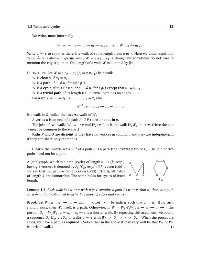
A (sub)graph, which is a path (cycle) of length k − 1 (k, resp.)having k vertices is denoted by Pk (Ck, resp.). If k is even (odd),we say that the path or cycle is even (odd). Clearly, all pathsof length k are isomorphic. The same holds for cycles of fixedlength. P5 C6
Lemma 1.3. Each walk W : u⋆−→ v with u 6= v contains a path P : u
⋆−→ v, that is, there is a path
P : u⋆−→ v that is obtained from W by removing edges and vertices.
Proof. Let W : u = u1 −→ . . . −→ uk+1 = v. Let i < j be indices such that ui = u j . If no suchi and j exist, then W , itself, is a path. Otherwise, in W = W1W2W3 : u
⋆−→ ui
⋆−→ u j
⋆−→ v the
portion U1 =W1W3 : u⋆−→ ui = u j
⋆−→ v is a shorter walk. By repeating this argument, we obtain
a sequence U1, U2, . . . , Um of walks u⋆−→ v with |W | > |U1| > · · · > |Um|. When the procedure
stops, we have a path as required. (Notice that in the above it may very well be that W1 or W3
is a trivial walk.) ⊓⊔
1.3 Paths and cycles 13
DEFINITION. If there exists a walk (and hence a path) from u to v in G, let
dG(u, v) =min{k | uk−→ v}
be the distance between u and v. If there are no walks u⋆−→ v, let dG(u, v) =∞ by convention.
A graph G is connected, if dG(u, v) <∞ for all u, v ∈ G; otherwise, it is disconnected. Themaximal connected subgraphs of G are its connected components. Denote
c(G) = the number of connected components of G .
If c(G) = 1, then G is, of course, connected.
The maximality condition means that a subgraph H ⊆ G is a connected component if andonly if H is connected and there are no edges leaving H, i.e., for every vertex v /∈ H, the subgraphG[VH ∪ {v}] is disconnected. Apparently, every connected component is an induced subgraph,and
N ∗G(v) = {u | dG(v,u) <∞}
is the connected component of G that contains v ∈ G. In particular, the connected componentsform a partition of G.
Shortest paths
DEFINITION. Let Gα be an edge weighted graph, that is, Gα is a graph G together with a weightfunction α: EG → R on its edges. For H ⊆ G, let
α(H) =∑
e∈H
α(e)
be the (total) weight of H. In particular, if P = e1e2 . . . ek is a path, then its weight is α(P) =∑ki=1α(ei). The minimum weighted distance between two vertices is
dαG(u, v) =min{α(P) | P : u⋆−→ v} .
In extremal problems we seek for optimal subgraphs H ⊆ G satisfying specific conditions. Inpractice we encounter situations where G might represent
• a distribution or transportation network (say, for mail), where the weights on edges aredistances, travel expenses, or rates of flow in the network;
• a system of channels in (tele)communication or computer architecture, where the weightspresent the rate of unreliability or frequency of action of the connections;
• a model of chemical bonds, where the weights measure molecular attraction.
1.3 Paths and cycles 14
In these examples we look for a subgraph with the smallest weight, and which connects twogiven vertices, or all vertices (if we want to travel around). On the other hand, if the graphrepresents a network of pipelines, the weights are volumes or capacities, and then one wantsto find a subgraph with the maximum weight.
We consider the minimum problem. For this, let G be a graph with an integer weight functionα: EG → N. In this case, call α(uv) the length of uv.
The shortest path problem: Given a connected graph G with a weight function α: EG → N, find
dαG(u, v) for given u, v ∈ G.
Assume that G is a connected graph. Dijkstra’s algorithm solves the problem for every pairu, v, where u is a fixed starting point and v ∈ G. Let us make the convention that α(uv) =∞,if uv /∈ G.
Dijkstra’s algorithm:
(i) Set u0 = u, t(u0) = 0 and t(v) =∞ for all v 6= u0.
(ii) For i ∈ [0,νG − 1]: for each v /∈ {u1, . . . ,ui},
replace t(v) by min{t(v), t(ui) +α(ui v)} .
Let ui+1 /∈ {u1, . . . ,ui} be any vertex with the least value t(ui+1).
(iii) Conclusion: dαG(u, v) = t(v).
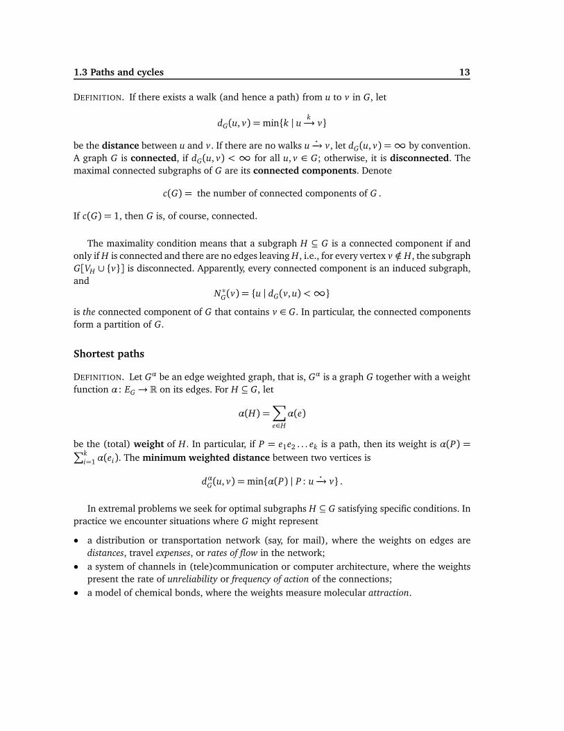
Example 1.7. Consider the following weighted graph G. Apply Dijkstra’s algorithm to the vertexv0.
• u0 = v0, t(u0) = 0, others are∞.
• t(v1) = min{∞, 2} = 2, t(v2) = min{∞, 3} = 3, othersare∞. Thus u1 = v1.
• t(v2) = min{3, t(u1) + α(u1v2)} = min{3,4} = 3, t(v3) =
2+ 1 = 3, t(v4) = 2+ 3 = 5, t(v5) = 2+ 2 = 4. Thus chooseu2 = v3.
• t(v2) =min{3,∞} = 3, t(v4) =min{5,3+ 2}= 5, t(v5) =
min{4,3+ 1}= 4. Thus set u3 = v2.
v0
v1
v2
v3
v4
v5
2
3
1
3 2
1
2
1
2
2
• t(v4) =min{5,3+ 1}= 4, t(v5) =min{4,∞} = 4. Thus choose u4 = v4.
• t(v5) =min{4,4+ 1}= 4. The algorithm stops.
We have obtained:
t(v1) = 2, t(v2) = 3, t(v3) = 3, t(v4) = 4, t(v5) = 4 .
These are the minimal weights from v0 to each vi.
1.3 Paths and cycles 15
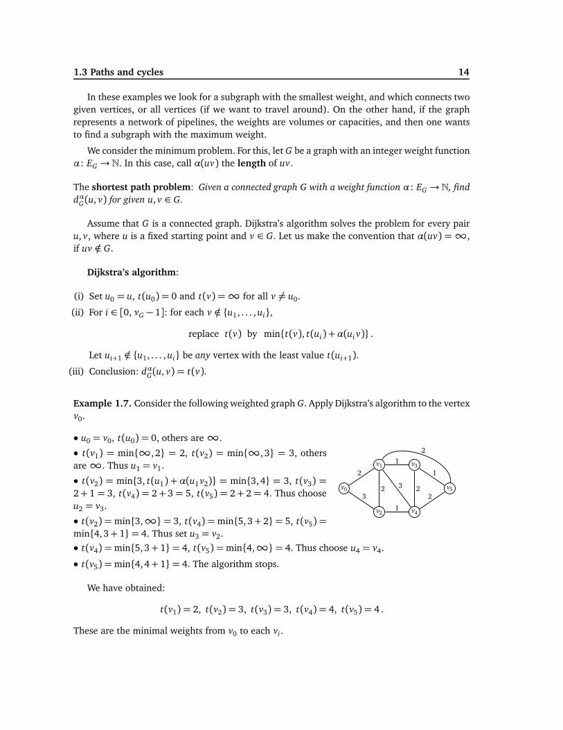
The steps of the algorithm can also be rewritten as a table:
v1 2 - - - -v2 3 3 3 - -v3 ∞ 3 - - -v4 ∞ 5 5 4 -v5 ∞ 4 4 4 4
The correctness of Dijkstra’s algorithm can verified be as follows.Let v ∈ V be any vertex, and let P : u0
⋆−→ u
⋆−→ v be a shortest path from u0 to v, where u
is any vertex u 6= v on such a path, possibly u = u0. Then, clearly, the first part of the path,u0
⋆−→ u, is a shortest path from u0 to u, and the latter part u
⋆−→ v is a shortest path from u to
v. Therefore, the length of the path P equals the sum of the weights of u0⋆−→ u and u
⋆−→ v.
Dijkstra’s algorithm makes use of this observation iteratively.
2
Connectivity of Graphs
2.1 Bipartite graphs and trees
In problems such as the shortest path problem we look for minimum solutions that satisfy thegiven requirements. The solutions in these cases are usually subgraphs without cycles. Suchconnected graphs will be called trees, and they are used, e.g., in search algorithms for databases.For concrete applications in this respect, see
T.H. CORMEN, C.E. LEISERSON AND R.L. RIVEST, “Introduction to Algorithms”, MIT Press, 1993.
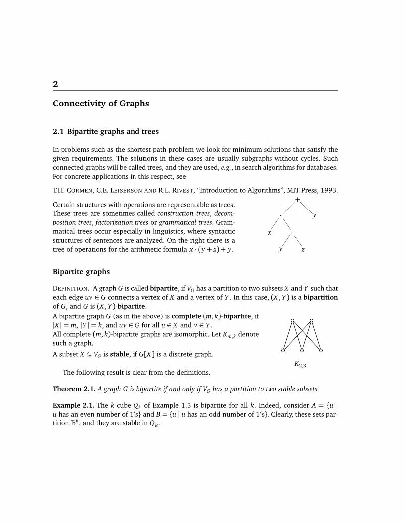
Certain structures with operations are representable as trees.These trees are sometimes called construction trees, decom-
position trees, factorization trees or grammatical trees. Gram-matical trees occur especially in linguistics, where syntacticstructures of sentences are analyzed. On the right there is atree of operations for the arithmetic formula x · (y + z) + y.
+
·
x +
y z
y
Bipartite graphs
DEFINITION. A graph G is called bipartite, if VG has a partition to two subsets X and Y such thateach edge uv ∈ G connects a vertex of X and a vertex of Y . In this case, (X , Y ) is a bipartitionof G, and G is (X , Y )-bipartite.
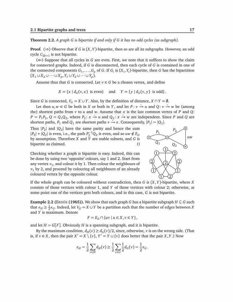
A bipartite graph G (as in the above) is complete (m, k)-bipartite, if|X | = m, |Y | = k, and uv ∈ G for all u ∈ X and v ∈ Y .All complete (m, k)-bipartite graphs are isomorphic. Let Km,k denotesuch a graph.
A subset X ⊆ VG is stable, if G[X ] is a discrete graph.K2,3
The following result is clear from the definitions.
Theorem 2.1. A graph G is bipartite if and only if VG has a partition to two stable subsets.
Example 2.1. The k-cube Qk of Example 1.5 is bipartite for all k. Indeed, consider A = {u |
u has an even number of 1′s} and B = {u | u has an odd number of 1′s}. Clearly, these sets par-tition Bk, and they are stable in Qk.
2.1 Bipartite graphs and trees 17
Theorem 2.2. A graph G is bipartite if and only if G it has no odd cycles (as subgraph).
Proof. (⇒) Observe that if G is (X , Y )-bipartite, then so are all its subgraphs. However, an oddcycle C2k+1 is not bipartite.
(⇐) Suppose that all cycles in G are even. First, we note that it suffices to show the claimfor connected graphs. Indeed, if G is disconnected, then each cycle of G is contained in one ofthe connected components G1, . . . , Gp of G. If Gi is (X i, Yi)-bipartite, then G has the bipartition(X1 ∪ X2 ∪ · · · ∪ X p, Y1 ∪ Y2 ∪ · · · ∪ Yp).
Assume thus that G is connected. Let v ∈ G be a chosen vertex, and define
X = {x | dG(v, x) is even} and Y = {y | dG(v, y) is odd} .
Since G is connected, VG = X ∪ Y . Also, by the definition of distance, X ∩ Y = ;.Let then u, w ∈ G be both in X or both in Y , and let P : v
⋆−→ u and Q : v
⋆−→ w be (among
the) shortest paths from v to u and w. Assume that x is the last common vertex of P and Q:P = P1P2, Q = Q1Q2, where P2 : x
⋆−→ u and Q2 : x
⋆−→ w are independent. Since P and Q are
shortest paths, P1 and Q1 are shortest paths v⋆−→ x . Consequently, |P1| = |Q1|.
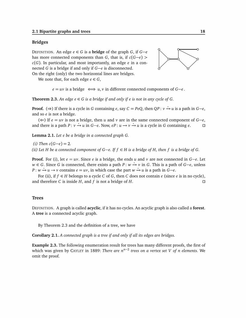
Thus |P2| and |Q2| have the same parity and hence the sum|P2|+ |Q2| is even, i.e., the path P−1
2 Q2 is even, and so uw /∈ EG
by assumption. Therefore X and Y are stable subsets, and G isbipartite as claimed. ⊓⊔
v x
u
w
P1
Q1
P2
Q2
uw
Checking whether a graph is bipartite is easy. Indeed, this canbe done by using two ‘opposite’ colours, say 1 and 2. Start fromany vertex v1, and colour it by 1. Then colour the neighbours ofv1 by 2, and proceed by colouring all neighbours of an alreadycoloured vertex by the opposite colour.
12
2
1
21
1
2
1
2
If the whole graph can be coloured without contradiction, then G is (X , Y )-bipartite, where X
consists of those vertices with colour 1, and Y of those vertices with colour 2; otherwise, atsome point one of the vertices gets both colours, and in this case, G is not bipartite.
Example 2.2 (ERDÖS (1965)). We show that each graph G has a bipartite subgraph H ⊆ G suchthat ǫH ≥
12ǫG. Indeed, let VG = X ∪ Y be a partition such that the number of edges between X
and Y is maximum. DenoteF = EG ∩ {uv | u ∈ X , v ∈ Y } ,
and let H = G[F]. Obviously H is a spanning subgraph, and it is bipartite.By the maximum condition, dH(v)≥ dG(v)/2, since, otherwise, v is on the wrong side. (That
is, if v ∈ X , then the pair X ′ = X \ {v}, Y ′ = Y ∪ {v} does better that the pair X , Y .) Now
ǫH =1
2
∑
v∈H
dH(v)≥1
2
∑
v∈G
1
2dG(v) =
1
2ǫG .
2.1 Bipartite graphs and trees 18
Bridges
DEFINITION. An edge e ∈ G is a bridge of the graph G, if G−e
has more connected components than G, that is, if c(G−e) >
c(G). In particular, and most importantly, an edge e in a con-nected G is a bridge if and only if G−e is disconnected.On the right (only) the two horizontal lines are bridges.
We note that, for each edge e ∈ G,
e = uv is a bridge ⇐⇒ u, v in different connected components of G−e .
Theorem 2.3. An edge e ∈ G is a bridge if and only if e is not in any cycle of G.
Proof. (⇒) If there is a cycle in G containing e, say C = PeQ, then QP : v⋆−→ u is a path in G−e,
and so e is not a bridge.(⇐) If e = uv is not a bridge, then u and v are in the same connected component of G−e,
and there is a path P : v⋆−→ u in G−e. Now, eP : u −→ v
⋆−→ u is a cycle in G containing e. ⊓⊔
Lemma 2.1. Let e be a bridge in a connected graph G.
(i) Then c(G−e) = 2.
(ii) Let H be a connected component of G−e. If f ∈ H is a bridge of H, then f is a bridge of G.
Proof. For (i), let e = uv. Since e is a bridge, the ends u and v are not connected in G−e. Letw ∈ G. Since G is connected, there exists a path P : w
⋆−→ v in G. This is a path of G−e, unless
P : w⋆−→ u→ v contains e = uv, in which case the part w
⋆−→ u is a path in G−e.
For (ii), if f ∈ H belongs to a cycle C of G, then C does not contain e (since e is in no cycle),and therefore C is inside H, and f is not a bridge of H. ⊓⊔
Trees
DEFINITION. A graph is called acyclic, if it has no cycles. An acyclic graph is also called a forest.A tree is a connected acyclic graph.
By Theorem 2.3 and the definition of a tree, we have
Corollary 2.1. A connected graph is a tree if and only if all its edges are bridges.
Example 2.3. The following enumeration result for trees has many different proofs, the first ofwhich was given by CAYLEY in 1889: There are nn−2 trees on a vertex set V of n elements. Weomit the proof.
2.1 Bipartite graphs and trees 19
On the other hand, there are only a few trees up to isomorphism:
n 1 2 3 4 5 6 7 8trees 1 1 1 2 3 6 11 23
n 9 10 11 12 13 14 15 16trees 47 106 235 551 1301 3159 7741 19 320
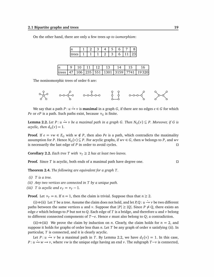
The nonisomorphic trees of order 6 are:
We say that a path P : u⋆−→ v is maximal in a graph G, if there are no edges e ∈ G for which
Pe or eP is a path. Such paths exist, because νG is finite.
Lemma 2.2. Let P : u⋆−→ v be a maximal path in a graph G. Then NG(v) ⊆ P. Moreover, if G is
acyclic, then dG(v) = 1.
Proof. If e = vw ∈ EG with w /∈ P, then also Pe is a path, which contradicts the maximalityassumption for P. Hence NG(v) ⊆ P. For acyclic graphs, if wv ∈ G, then w belongs to P, and wv
is necessarily the last edge of P in order to avoid cycles. ⊓⊔
Corollary 2.2. Each tree T with νT ≥ 2 has at least two leaves.
Proof. Since T is acyclic, both ends of a maximal path have degree one. ⊓⊔
Theorem 2.4. The following are equivalent for a graph T.
(i) T is a tree.
(ii) Any two vertices are connected in T by a unique path.
(iii) T is acyclic and ǫT = νT − 1.
Proof. Let νT = n. If n= 1, then the claim is trivial. Suppose thus that n≥ 2.
(i)⇒(ii) Let T be a tree. Assume the claim does not hold, and let P,Q : u⋆−→ v be two different
paths between the same vertices u and v. Suppose that |P| ≥ |Q|. Since P 6= Q, there exists anedge e which belongs to P but not to Q. Each edge of T is a bridge, and therefore u and v belongto different connected components of T−e. Hence e must also belong to Q; a contradiction.
(ii)⇒(iii) We prove the claim by induction on n. Clearly, the claim holds for n = 2, andsuppose it holds for graphs of order less than n. Let T be any graph of order n satisfying (ii). Inparticular, T is connected, and it is clearly acyclic.
Let P : u⋆−→ v be a maximal path in T . By Lemma 2.2, we have dT (v) = 1. In this case,
P : u⋆−→ w −→ v, where vw is the unique edge having an end v. The subgraph T−v is connected,
2.1 Bipartite graphs and trees 20
and it satisfies the condition (ii). By induction hypothesis, ǫT−v = n−2, and so ǫT = ǫT−v+1=n− 1, and the claim follows.
(iii)⇒(i) Assume (iii) holds for T . We need to show that T is connected. Indeed, let theconnected components of T be Ti = (Vi , Ei), for i ∈ [1, k]. Since T is acyclic, so are the connectedgraphs Ti, and hence they are trees, for which we have proved that |Ei| = |Vi | − 1. Now, νT =∑k
i=1 |Vi |, and ǫT =∑k
i=1 |Ei|. Therefore,
n− 1= ǫT =
k∑
i=1
(|Vi | − 1) =k∑
i=1
|Vi | − k = n− k ,
which gives that k = 1, that is, T is connected. ⊓⊔
Example 2.4. Consider a cup tournament of n teams. If during a round there are k teams leftin the tournament, then these are divided into ⌊k⌋ pairs, and from each pair only the winnercontinues. If k is odd, then one of the teams goes to the next round without having to play. Howmany plays are needed to determine the winner?
So if there are 14 teams, after the first round 7 teams continue, and after the second round4 teams continue, then 2. So 13 plays are needed in this example.
The answer to our problem is n− 1, since the cup tournament is a tree, where a play corre-sponds to an edge of the tree.
Spanning trees
Theorem 2.5. Each connected graph has a spanning tree, that is, a spanning graph that is a tree.
Proof. Let T ⊆ G be a maximum order subtree of G (i.e., subgraph that is a tree). If VT 6=
VG , there exists an edge uv /∈ EG such that u ∈ T and v /∈ T . But then T is not maximal; acontradiction. ⊓⊔
Corollary 2.3. For each connected graph G, ǫG ≥ νG −1. Moreover, a connected graph G is a tree
if and only if ǫG = νG − 1.
Proof. Let T be a spanning tree of G. Then ǫG ≥ ǫT = νT −1= νG−1. The second claim is alsoclear. ⊓⊔
Example 2.5. In Shannon’s switching game a positive player P and a negative player N playon a graph G with two special vertices: a source s and a sink r. P and N alternate turns so thatP designates an edge by +, and N by −. Each edge can be designated at most once. It is P ’spurpose to designate a path s
⋆−→ r (that is, to designate all edges in one such path), and N tries
to block all paths s⋆−→ r (that is, to designate at least one edge in each such path). We say that
a game (G, s, r) is
• positive, if P has a winning strategy no matter who begins the game,• negative, if N has a winning strategy no matter who begins the game,
2.1 Bipartite graphs and trees 21
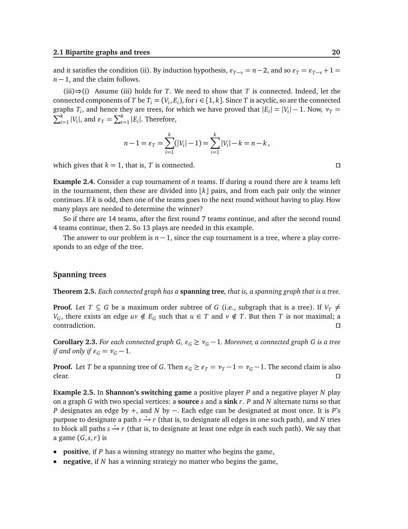
• neutral, if the winner depends on who begins the game.
The game on the right is neutral.
s
r
LEHMAN proved in 1964 that Shannon’s switching game (G, s, r) is positive if and only if there
exists H ⊆ G such that H contains s and r and H has two spanning trees with no edges in common.
In the other direction the claim can be proved along the following lines. Assume that thereexists a subgraph H containing s and r and that has two spanning trees with no edges in com-mon. Then P plays as follows. If N marks by − an edge from one of the two trees, then P marksby + an edge in the other tree such that this edge reconnects the broken tree. In this way, P
always has two spanning trees for the subgraph H with only edges marked by + in common.In converse the claim is considerably more difficult to prove.There remains the problem to characterize those Shannon’s switching games (G, s, r) that
are neutral (negative, respectively).
The connector problem
To build a network connecting n nodes (towns, computers, chips in a computer) it is desirable todecrease the cost of construction of the links to the minimum. This is the connector problem.In graph theoretical terms we wish to find an optimal spanning subgraph of a weighted graph.Such an optimal subgraph is clearly a spanning tree, for, otherwise a deletion of any nonbridgewill reduce the total weight of the subgraph.
Let then Gα be a graph G together with a weight function α: EG → R+ (positive reals) on
the edges. Kruskal’s algorithm (also known as the greedy algorithm) provides a solution to theconnector problem.Kruskal’s algorithm: For a connected and weighted graph Gα of order n:
(i) Let e1 be an edge of smallest weight, and set E1 = {e1}.
(ii) For each i = 2,3, . . . , n−1 in this order, choose an edge ei /∈ Ei−1 of smallest possible weightsuch that ei does not produce a cycle when added to G[Ei−1], and let Ei = Ei−1 ∪ {ei}.
The final outcome is T = (VG , En−1).
By the construction, T = (VG , En−1) is a spanning tree of G, because it contains no cycles, itis connected and has n− 1 edges. We now show that T has the minimum total weight amongthe spanning trees of G.
Suppose T1 is any spanning tree of G. Let ek be the first edge produced by the algorithm thatis not in T1. If we add ek to T1, then a cycle C containing ek is created. Also, C must containan edge e that is not in T . When we replace e by ek in T1, we still have a spanning tree, say
2.1 Bipartite graphs and trees 22
T2. However, by the construction, α(ek)≤ α(e), and therefore α(T2)≤ α(T1). Note that T2 hasmore edges in common with T than T1.
Repeating the above procedure, we can transform T1 to T by replacing edges, one by one,such that the total weight does not increase. We deduce that α(T ) ≤ α(T1).
The outcome of Kruskal’s algorithm need not be unique. Indeed, there may exist severaloptimal spanning trees (with the same weight, of course) for a graph.
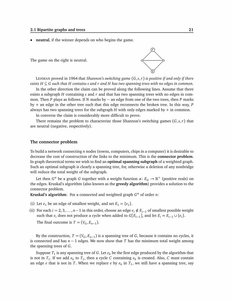
Example 2.6. When applied to the weighted graph on theright, the algorithm produces the sequence: e1 = v2v4,e2 = v4v5, e3 = v3v6, e4 = v2v3 and e5 = v1v2. The to-tal weight of the spanning tree is thus 9.Also, the selection e1 = v2v5, e2 = v4v5, e3 = v5v6, e4 =
v3v6, e5 = v1v2 gives another optimal solution (of weight9).
v1 v2 v3
v4 v5 v6
3
4
2
1
122
21 2
3
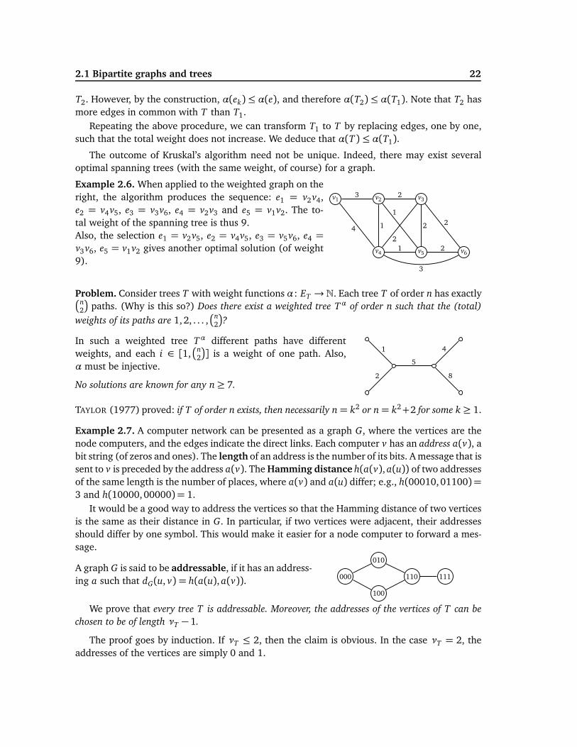
Problem. Consider trees T with weight functions α: ET → N. Each tree T of order n has exactly�n2
�paths. (Why is this so?) Does there exist a weighted tree Tα of order n such that the (total)
weights of its paths are 1,2, . . . ,�
n2
�?
In such a weighted tree Tα different paths have differentweights, and each i ∈ [1,
�n2
�] is a weight of one path. Also,
α must be injective.
No solutions are known for any n≥ 7.2
1
5
8
4
TAYLOR (1977) proved: if T of order n exists, then necessarily n= k2 or n= k2+2 for some k ≥ 1.
Example 2.7. A computer network can be presented as a graph G, where the vertices are thenode computers, and the edges indicate the direct links. Each computer v has an address a(v), abit string (of zeros and ones). The length of an address is the number of its bits. A message that issent to v is preceded by the address a(v). The Hamming distance h(a(v), a(u)) of two addressesof the same length is the number of places, where a(v) and a(u) differ; e.g., h(00010,01100) =3 and h(10000,00000) = 1.
It would be a good way to address the vertices so that the Hamming distance of two verticesis the same as their distance in G. In particular, if two vertices were adjacent, their addressesshould differ by one symbol. This would make it easier for a node computer to forward a mes-sage.
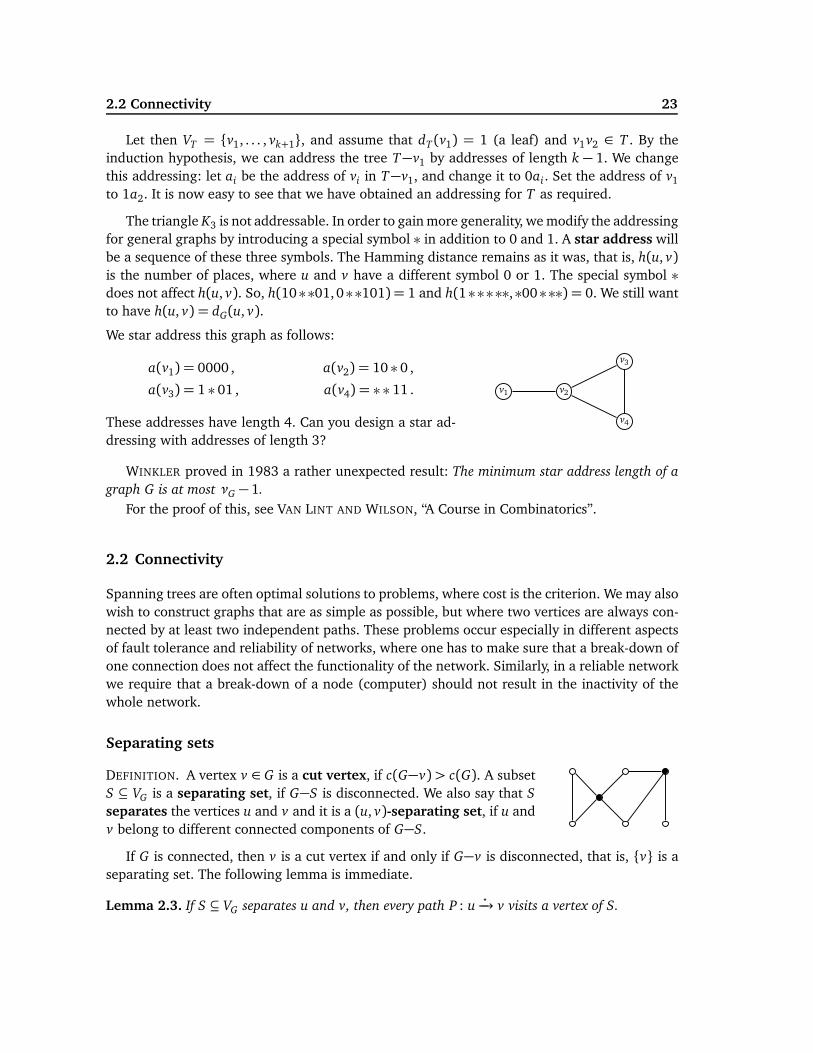
A graph G is said to be addressable, if it has an address-ing a such that dG(u, v) = h(a(u), a(v)). 000
100
010
110 111
We prove that every tree T is addressable. Moreover, the addresses of the vertices of T can be
chosen to be of length νT − 1.
The proof goes by induction. If νT ≤ 2, then the claim is obvious. In the case νT = 2, theaddresses of the vertices are simply 0 and 1.
2.2 Connectivity 23
Let then VT = {v1, . . . , vk+1}, and assume that dT (v1) = 1 (a leaf) and v1v2 ∈ T . By theinduction hypothesis, we can address the tree T−v1 by addresses of length k − 1. We changethis addressing: let ai be the address of vi in T−v1, and change it to 0ai. Set the address of v1
to 1a2. It is now easy to see that we have obtained an addressing for T as required.
The triangle K3 is not addressable. In order to gain more generality, we modify the addressingfor general graphs by introducing a special symbol ∗ in addition to 0 and 1. A star address willbe a sequence of these three symbols. The Hamming distance remains as it was, that is, h(u, v)
is the number of places, where u and v have a different symbol 0 or 1. The special symbol ∗does not affect h(u, v). So, h(10∗∗01,0∗∗101) = 1 and h(1∗∗∗∗∗,∗00∗∗∗) = 0. We still wantto have h(u, v) = dG(u, v).
We star address this graph as follows:
a(v1) = 0000 , a(v2) = 10 ∗ 0 ,
a(v3) = 1 ∗ 01 , a(v4) = ∗ ∗ 11 .
These addresses have length 4. Can you design a star ad-dressing with addresses of length 3?
v1 v2
v3
v4
WINKLER proved in 1983 a rather unexpected result: The minimum star address length of a
graph G is at most νG − 1.
For the proof of this, see VAN LINT AND WILSON, “A Course in Combinatorics”.
2.2 Connectivity
Spanning trees are often optimal solutions to problems, where cost is the criterion. We may alsowish to construct graphs that are as simple as possible, but where two vertices are always con-nected by at least two independent paths. These problems occur especially in different aspectsof fault tolerance and reliability of networks, where one has to make sure that a break-down ofone connection does not affect the functionality of the network. Similarly, in a reliable networkwe require that a break-down of a node (computer) should not result in the inactivity of thewhole network.
Separating sets
DEFINITION. A vertex v ∈ G is a cut vertex, if c(G−v)> c(G). A subsetS ⊆ VG is a separating set, if G−S is disconnected. We also say that S
separates the vertices u and v and it is a (u, v)-separating set, if u andv belong to different connected components of G−S.
If G is connected, then v is a cut vertex if and only if G−v is disconnected, that is, {v} is aseparating set. The following lemma is immediate.
Lemma 2.3. If S ⊆ VG separates u and v, then every path P : u⋆−→ v visits a vertex of S.
2.2 Connectivity 24
Lemma 2.4. If a connected graph G has no separating sets, then it is a complete graph.
Proof. If νG ≤ 2, then the claim is clear. For νG ≥ 3, assume that G is not complete, and letuv /∈ G. Now VG \ {u, v} is a separating set. The claim follows from this. ⊓⊔
DEFINITION. The (vertex) connectivity number κ(G) of G is defined as
κ(G) =min{k | k = |S|, G−S disconnected or trivial,S ⊆ VG} .
A graph G is k-connected, if κ(G) ≥ k.
In other words,
• κ(G) = 0, if G is disconnected,• κ(G) = νG − 1, if G is a complete graph, and• otherwise κ(G) equals the minimum size of a separating set of G.
Clearly, if G is connected, then it is 1-connected.
DEFINITION. An edge cut F of G consists of edges so that G−F is disconnected. Let
κ′(G) =min{k | k = |F |, G−F disconnected, F ⊆ EG} .
For trivial graphs, let κ′(G) = 0. A graph G is k-edge connected, if κ′(G) ≥ k. A minimaledge cut F ⊆ EG is a bond (F \ {e} is not an edge cut for any e ∈ F).
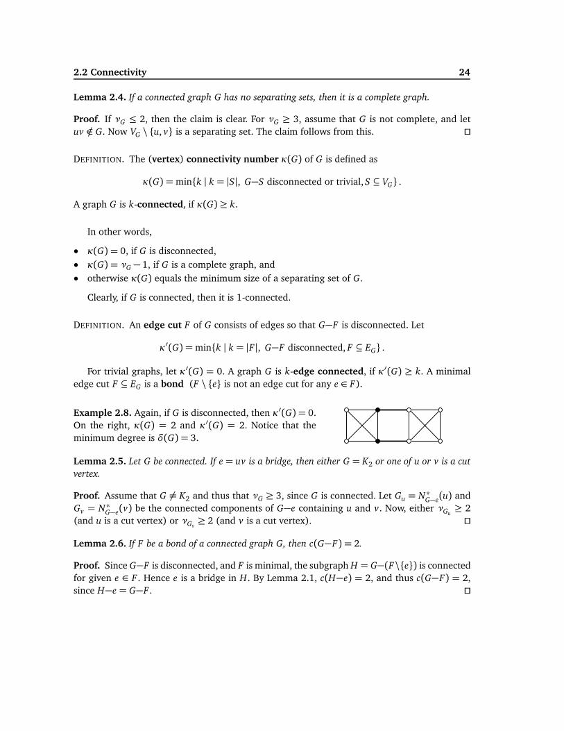
Example 2.8. Again, if G is disconnected, then κ′(G) = 0.On the right, κ(G) = 2 and κ′(G) = 2. Notice that theminimum degree is δ(G) = 3.
Lemma 2.5. Let G be connected. If e = uv is a bridge, then either G = K2 or one of u or v is a cut
vertex.
Proof. Assume that G 6= K2 and thus that νG ≥ 3, since G is connected. Let Gu = N ∗G−e(u) andGv = N ∗G−e(v) be the connected components of G−e containing u and v. Now, either νGu
≥ 2(and u is a cut vertex) or νGv
≥ 2 (and v is a cut vertex). ⊓⊔
Lemma 2.6. If F be a bond of a connected graph G, then c(G−F) = 2.
Proof. Since G−F is disconnected, and F is minimal, the subgraph H = G−(F\{e}) is connectedfor given e ∈ F . Hence e is a bridge in H. By Lemma 2.1, c(H−e) = 2, and thus c(G−F) = 2,since H−e = G−F . ⊓⊔
2.2 Connectivity 25
Theorem 2.6 (WHITNEY (1932)). For any graph G,
κ(G) ≤ κ′(G) ≤ δ(G) .
Proof. Assume G is nontrivial. Clearly, κ′(G) ≤ δ(G), since if we remove all edges with an endv, we disconnect G. If κ′(G) = 0, then G is disconnected, and in this case also κ(G) = 0. Ifκ′(G) = 1, then G is connected and contains a bridge. By Lemma 2.5, either G = K2 or G has acut vertex. In both of these cases, also κ(G) = 1.
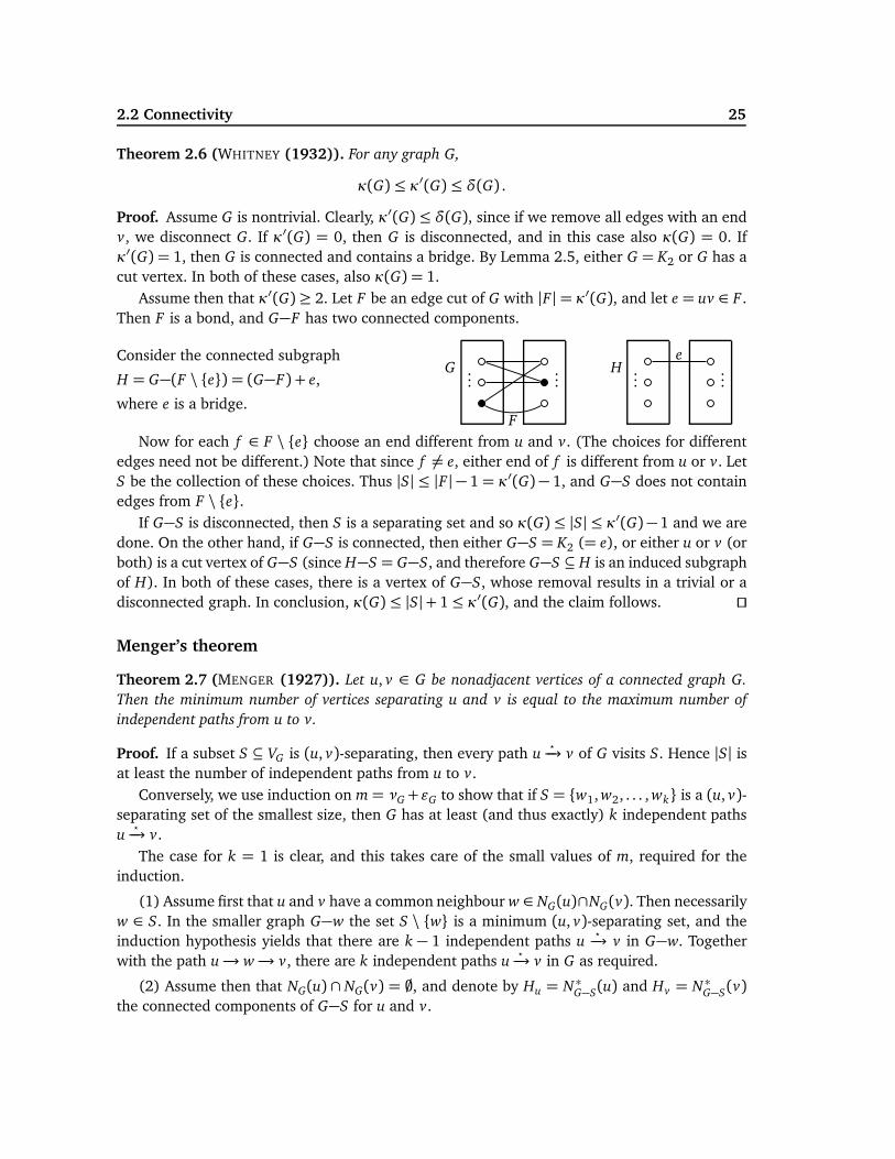
Assume then that κ′(G) ≥ 2. Let F be an edge cut of G with |F | = κ′(G), and let e = uv ∈ F .Then F is a bond, and G−F has two connected components.
Consider the connected subgraph
H = G−(F \ {e}) = (G−F) + e,
where e is a bridge.
......
G
F
......
He
Now for each f ∈ F \ {e} choose an end different from u and v. (The choices for differentedges need not be different.) Note that since f 6= e, either end of f is different from u or v. LetS be the collection of these choices. Thus |S| ≤ |F | − 1 = κ′(G)− 1, and G−S does not containedges from F \ {e}.
If G−S is disconnected, then S is a separating set and so κ(G) ≤ |S| ≤ κ′(G)−1 and we aredone. On the other hand, if G−S is connected, then either G−S = K2 (= e), or either u or v (orboth) is a cut vertex of G−S (since H−S = G−S, and therefore G−S ⊆ H is an induced subgraphof H). In both of these cases, there is a vertex of G−S, whose removal results in a trivial or adisconnected graph. In conclusion, κ(G) ≤ |S|+ 1≤ κ′(G), and the claim follows. ⊓⊔
Menger’s theorem
Theorem 2.7 (MENGER (1927)). Let u, v ∈ G be nonadjacent vertices of a connected graph G.
Then the minimum number of vertices separating u and v is equal to the maximum number of
independent paths from u to v.
Proof. If a subset S ⊆ VG is (u, v)-separating, then every path u⋆−→ v of G visits S. Hence |S| is
at least the number of independent paths from u to v.Conversely, we use induction on m = νG+ǫG to show that if S = {w1, w2, . . . , wk} is a (u, v)-
separating set of the smallest size, then G has at least (and thus exactly) k independent pathsu
⋆−→ v.
The case for k = 1 is clear, and this takes care of the small values of m, required for theinduction.
(1) Assume first that u and v have a common neighbour w ∈ NG(u)∩NG(v). Then necessarilyw ∈ S. In the smaller graph G−w the set S \ {w} is a minimum (u, v)-separating set, and theinduction hypothesis yields that there are k − 1 independent paths u
⋆−→ v in G−w. Together
with the path u −→ w −→ v, there are k independent paths u⋆−→ v in G as required.
(2) Assume then that NG(u) ∩ NG(v) = ;, and denote by Hu = N ∗G−S(u) and Hv = N ∗G−S(v)
the connected components of G−S for u and v.
2.2 Connectivity 26
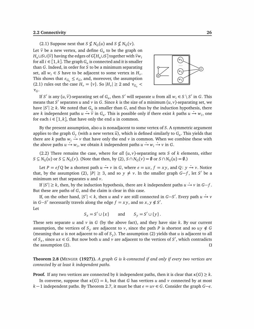
(2.1) Suppose next that S * NG(u) and S * NG(v).
Let bv be a new vertex, and define Gu to be the graph onHu∪S∪{bv} having the edges of G[Hu∪S] together with bvwi
for all i ∈ [1, k]. The graph Gu is connected and it is smallerthan G. Indeed, in order for S to be a minimum separatingset, all wi ∈ S have to be adjacent to some vertex in Hv .This shows that ǫGu
≤ ǫG, and, moreover, the assumption(2.1) rules out the case Hv = {v}. So |Hv| ≥ 2 and νGu
<
νG .
u
bv
w1
w2
. . .
wk
If S′ is any (u,bv)-separating set of Gu, then S′ will separate u from all wi ∈ S \ S′ in G. Thismeans that S′ separates u and v in G. Since k is the size of a minimum (u, v)-separating set, wehave |S′| ≥ k. We noted that Gu is smaller than G, and thus by the induction hypothesis, thereare k independent paths u
⋆−→ bv in Gu. This is possible only if there exist k paths u
⋆−→ wi , one
for each i ∈ [1, k], that have only the end u in common.
By the present assumption, also u is nonadjacent to some vertex of S. A symmetric argumentapplies to the graph Gv (with a new vertex bu), which is defined similarly to Gu. This yields thatthere are k paths wi
⋆−→ v that have only the end v in common. When we combine these with
the above paths u⋆−→ wi , we obtain k independent paths u
⋆−→ wi
⋆−→ v in G.
(2.2) There remains the case, where for all (u, v)-separating sets S of k elements, eitherS ⊆ NG(u) or S ⊆ NG(v). (Note that then, by (2), S ∩ NG(v) = ; or S ∩ NG(u) = ;.)
Let P = e f Q be a shortest path u⋆−→ v in G, where e = ux , f = x y, and Q : y
⋆−→ v. Notice
that, by the assumption (2), |P| ≥ 3, and so y 6= v. In the smaller graph G− f , let S′ be aminimum set that separates u and v.
If |S′| ≥ k, then, by the induction hypothesis, there are k independent paths u⋆−→ v in G− f .
But these are paths of G, and the claim is clear in this case.If, on the other hand, |S′| < k, then u and v are still connected in G−S′. Every path u
⋆−→ v
in G−S′ necessarily travels along the edge f = x y, and so x , y /∈ S′.Let
Sx = S′ ∪ {x} and Sy = S′ ∪ {y} .
These sets separate u and v in G (by the above fact), and they have size k. By our currentassumption, the vertices of Sy are adjacent to v, since the path P is shortest and so uy /∈ G
(meaning that u is not adjacent to all of Sy). The assumption (2) yields that u is adjacent to allof Sx , since ux ∈ G. But now both u and v are adjacent to the vertices of S′, which contradictsthe assumption (2). ⊓⊔
Theorem 2.8 (MENGER (1927)). A graph G is k-connected if and only if every two vertices are
connected by at least k independent paths.
Proof. If any two vertices are connected by k independent paths, then it is clear that κ(G) ≥ k.In converse, suppose that κ(G) = k, but that G has vertices u and v connected by at most
k−1 independent paths. By Theorem 2.7, it must be that e = uv ∈ G. Consider the graph G−e.
2.2 Connectivity 27
Now u and v are connected by at most k − 2 independent paths in G−e, and by Theorem 2.7,u and v can be separated in G−e by a set S with |S| = k− 2. Since νG > k (because κ(G) = k),there exists a w ∈ G that is not in S ∪ {u, v}. The vertex w is separated in G−e by S from u
or from v; otherwise there would be a path u⋆−→ v in (G−e)−S. Say, this vertex is u. The set
S ∪ {v} has k − 1 elements, and it separates u from w in G, which contradicts the assumptionthat κ(G) = k. This proves the claim. ⊓⊔
We state without a proof the corresponding separation property for edge connectivity.
DEFINITION. Let G be a graph. A uv-disconnecting set is a set F ⊆ EG such that every pathu
⋆−→ v contains an edge from F .
Theorem 2.9. Let u, v ∈ G with u 6= v in a graph G. Then the maximum number of edge-disjoint
paths u⋆−→ v equals the minimum number k of edges in a uv-disconnecting set.
Corollary 2.4. A graph G is k-edge connected if and only if every two vertices are connected by at
least k edge disjoint paths.
Example 2.9. Recall the definition of the cube Qk from Example 1.5. We show that κ(Qk) = k.First of all, κ(Qk) ≤ δ(Qk) = k. In converse, we show the claim by induction. Extract from
Qk the disjoint subgraphs: G0 induced by {0u | u ∈ Bk−1} and G1 induced by {1u | u ∈ Bk−1}.These are (isomorphic to) Qk−1, and Qk is obtained from the union of G0 and G1 by adding the2k−1 edges (0u, 1u) for all u ∈ Bk−1.
Let S be a separating set of Qk with |S| ≤ k. If both G0−S and G1−S were connected,also Qk−S would be connected, since one pair (0u, 1u) necessarily remains in Qk−S. So wecan assume that G0−S is disconnected. (The case for G1−S is symmetric.) By the inductionhypothesis, κ(G0) = k−1, and hence S contains at least k−1 vertices of G0 (and so |S| ≥ k−1).If there were no vertices from G1 in S, then, of course, G1−S is connected, and the edges (0u, 1u)
of Qk would guarantee that Qk−S is connected; a contradiction. Hence |S| ≥ k.
Example 2.10. We have κ′(Qk) = k for the k-cube. Indeed, by Whitney’s theorem, κ(G) ≤κ′(G) ≤ δ(G). Since κ(Qk) = k = δ(Qk), also κ′(Qk) = k.
Algorithmic Problem. The connectivity problems tend to be algorithmically difficult. In thedisjoint paths problem we are given a set (ui, vi) of pairs of vertices for i = 1,2, . . . , k, and itis asked whether there exist paths Pi : ui
⋆−→ vi that have no vertices in common. This problem
was shown to be NP-complete by KNUTH in 1975. (However, for fixed k, the problem has a fastalgorithm due to ROBERTSON and SEYMOUR (1986).)
2.2 Connectivity 28
Dirac’s fans
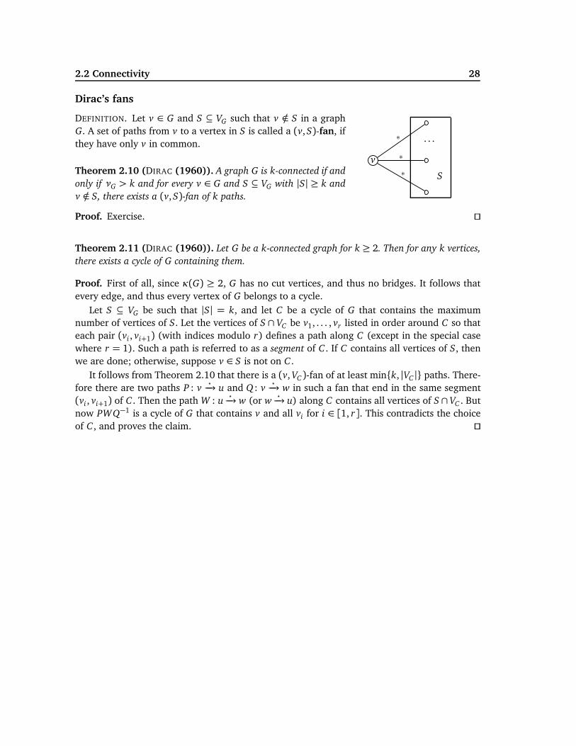
DEFINITION. Let v ∈ G and S ⊆ VG such that v /∈ S in a graphG. A set of paths from v to a vertex in S is called a (v,S)-fan, ifthey have only v in common.
Theorem 2.10 (DIRAC (1960)). A graph G is k-connected if and
only if νG > k and for every v ∈ G and S ⊆ VG with |S| ≥ k and
v /∈ S, there exists a (v,S)-fan of k paths.
v
. . .
∗
∗
∗
S
Proof. Exercise. ⊓⊔
Theorem 2.11 (DIRAC (1960)). Let G be a k-connected graph for k ≥ 2. Then for any k vertices,
there exists a cycle of G containing them.
Proof. First of all, since κ(G) ≥ 2, G has no cut vertices, and thus no bridges. It follows thatevery edge, and thus every vertex of G belongs to a cycle.
Let S ⊆ VG be such that |S| = k, and let C be a cycle of G that contains the maximumnumber of vertices of S. Let the vertices of S ∩ VC be v1, . . . , vr listed in order around C so thateach pair (vi , vi+1) (with indices modulo r) defines a path along C (except in the special casewhere r = 1). Such a path is referred to as a segment of C . If C contains all vertices of S, thenwe are done; otherwise, suppose v ∈ S is not on C .
It follows from Theorem 2.10 that there is a (v, VC )-fan of at least min{k, |VC |} paths. There-fore there are two paths P : v
⋆−→ u and Q : v
⋆−→ w in such a fan that end in the same segment
(vi , vi+1) of C . Then the path W : u⋆−→ w (or w
⋆−→ u) along C contains all vertices of S ∩ VC . But
now PWQ−1 is a cycle of G that contains v and all vi for i ∈ [1, r]. This contradicts the choiceof C , and proves the claim. ⊓⊔
3
Tours and Matchings
3.1 Eulerian graphs
The first proper problem in graph theory was the Königsberg bridge problem. In general, thisproblem concerns of travelling in a graph such that one tries to avoid using any edge twice.In practice these eulerian problems occur, for instance, in optimizing distribution networks –such as delivering mail, where in order to save time each street should be travelled only once.The same problem occurs in mechanical graph plotting, where one avoids lifting the pen off thepaper while drawing the lines.
Euler tours
DEFINITION. A walk W = e1e2 . . . en is a trail, if ei 6= e j for all i 6= j. An Euler trail of a graphG is a trail that visits every edge once. A connected graph G is eulerian, if it has a closed trailcontaining every edge of G. Such a trail is called an Euler tour.
Notice that if W = e1e2 . . . en is an Euler tour (and so EG = {e1, e2, . . . , en}), also eiei+1 . . . ene1 . . . ei−1
is an Euler tour for all i ∈ [1, n]. A complete proof of the following Euler’s Theorem was firstgiven by HIERHOLZER in 1873.
Theorem 3.1 (EULER (1736), HIERHOLZER (1873)). A connected graph G is eulerian if and only
if every vertex has an even degree.
Proof. (⇒) Suppose W : u⋆−→ u is an Euler tour. Let v (6= u) be a vertex that occurs k times in
W . Every time an edge arrives at v, another edge departs from v, and therefore dG(v) = 2k.Also, dG(u) is even, since W starts and ends at u.
(⇐) Assume G is a nontrivial connected graph such that dG(v) is even for all v ∈ G. Let
W = e1e2 . . . en : v0⋆−→ vn with ei = vi−1vi
be a longest trail in G. It follows that all e = vnw ∈ G are among the edges of W , for, otherwise,W could be prolonged to We. In particular, v0 = vn, that is, W is a closed trail. (Indeed, if itwere vn 6= v0 and vn occurs k times in W , then dG(vn) = 2(k− 1) + 1 and that would be odd.)
If W is not an Euler tour, then, since G is connected, there exists an edge f = viu ∈ G forsome i, which is not in W . However, now
ei+1 . . . ene1 . . . ei f
is a trail in G, and it is longer than W . This contradiction to the choice of W proves the claim.⊓⊔
Example 3.1. The k-cube Qk is eulerian for even integers k, because Qk is k-regular.
3.1 Eulerian graphs 30
Theorem 3.2. A connected graph has an Euler trail if and only if it has at most two vertices of odd
degree.
Proof. If G has an Euler trail u⋆−→ v, then, as in the proof of Theorem 3.1, each vertex w /∈ {u, v}
has an even degree.Assume then that G is connected and has at most two vertices of odd degree. If G has no
vertices of odd degree then, by Theorem 3.1, G has an Euler trail. Otherwise, by the handshakinglemma, every graph has an even number of vertices with odd degree, and therefore G has exactlytwo such vertices, say u and v. Let H be a graph obtained from G by adding a vertex w, andthe edges uw and vw. In H every vertex has an even degree, and hence it has an Euler tour, sayu
⋆−→ v −→ w −→ u. Here the beginning part u
⋆−→ v is an Euler trail of G. ⊓⊔
The Chinese postman
The following problem is due to GUAN MEIGU (1962). Consider a village, where a postmanwishes to plan his route to save the legs, but still every street has to be walked through. Thisproblem is akin to Euler’s problem and to the shortest path problem.
Let G be a graph with a weight function α: EG → R+. The Chinese postman problem is to
find a minimum weighted tour in G (starting from a given vertex, the post office).If G is eulerian, then any Euler tour will do as a solution, because such a tour traverses each
edge exactly once and this is the best one can do. In this case the weight of the optimal tour isthe total weight of the graph G, and there is a good algorithm for finding such a tour:
Fleury’s algorithm:
• Let v0 ∈ G be a chosen vertex, and let W0 be the trivial path on v0.• Repeat the following procedure for i = 1,2, . . . as long as possible: suppose a trail Wi =
e1e2 . . . ei has been constructed, where e j = v j−1v j.Choose an edge ei+1 (6= e j for j ∈ [1, i]) so that
(i) ei+1 has an end vi, and(ii)ei+1 is not a bridge of Gi = G−{e1, . . . , ei}, unless there is no alternative.
Notice that, as is natural, the weights α(e) play no role in the eulerian case.
Theorem 3.3. If G is eulerian, then any trail of G constructed by Fleury’s algorithm is an Euler
tour of G.
Proof. Exercise. ⊓⊔
If G is not eulerian, the poor postman has to walk at least one street twice. This happens, e.g.,if one of the streets is a dead end, and in general if there is a street corner of an odd numberof streets. We can attack this case by reducing it to the eulerian case as follows. An edge e = uv
will be duplicated, if it is added to G parallel to an existing edge e′ = uv with the same weight,α(e′) = α(e).
3.2 Hamiltonian graphs 31
2
4
1
33
2 2 2
4
1
33
2 2 2
4
1
3
3
3
2
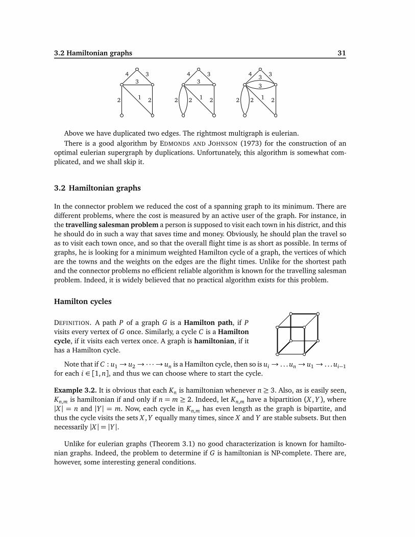
Above we have duplicated two edges. The rightmost multigraph is eulerian.There is a good algorithm by EDMONDS AND JOHNSON (1973) for the construction of an
optimal eulerian supergraph by duplications. Unfortunately, this algorithm is somewhat com-plicated, and we shall skip it.
3.2 Hamiltonian graphs
In the connector problem we reduced the cost of a spanning graph to its minimum. There aredifferent problems, where the cost is measured by an active user of the graph. For instance, inthe travelling salesman problem a person is supposed to visit each town in his district, and thishe should do in such a way that saves time and money. Obviously, he should plan the travel soas to visit each town once, and so that the overall flight time is as short as possible. In terms ofgraphs, he is looking for a minimum weighted Hamilton cycle of a graph, the vertices of whichare the towns and the weights on the edges are the flight times. Unlike for the shortest pathand the connector problems no efficient reliable algorithm is known for the travelling salesmanproblem. Indeed, it is widely believed that no practical algorithm exists for this problem.
Hamilton cycles
DEFINITION. A path P of a graph G is a Hamilton path, if P
visits every vertex of G once. Similarly, a cycle C is a Hamiltoncycle, if it visits each vertex once. A graph is hamiltonian, if ithas a Hamilton cycle.
Note that if C : u1→ u2→ · · · → un is a Hamilton cycle, then so is ui → . . . un→ u1→ . . . ui−1
for each i ∈ [1, n], and thus we can choose where to start the cycle.
Example 3.2. It is obvious that each Kn is hamiltonian whenever n≥ 3. Also, as is easily seen,Kn,m is hamiltonian if and only if n = m ≥ 2. Indeed, let Kn,m have a bipartition (X , Y ), where|X | = n and |Y | = m. Now, each cycle in Kn,m has even length as the graph is bipartite, andthus the cycle visits the sets X , Y equally many times, since X and Y are stable subsets. But thennecessarily |X |= |Y |.
Unlike for eulerian graphs (Theorem 3.1) no good characterization is known for hamilto-nian graphs. Indeed, the problem to determine if G is hamiltonian is NP-complete. There are,however, some interesting general conditions.
3.2 Hamiltonian graphs 32
Lemma 3.1. If G is hamiltonian, then for every nonempty subset S ⊆ VG ,
c(G−S) ≤ |S| .
Proof. Let ; 6= S ⊆ VG , u ∈ S, and let C : u⋆−→ u be a Hamilton cycle of G. Assume G−S has k
connected components, Gi, i ∈ [1, k]. The case k = 1 is trivial, and hence suppose that k > 1.Let ui be the last vertex of C that belongs to Gi , and let vi be the vertex that follows ui in C .Now vi ∈ S for each i by the choice of ui , and v j 6= vt for all j 6= t, because C is a cycle andui vi ∈ G for all i. Thus |S| ≥ k as required. ⊓⊔
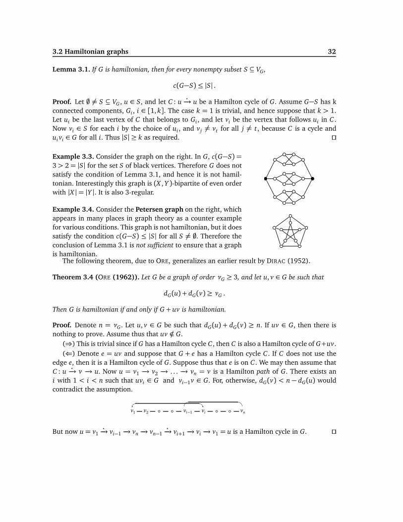
Example 3.3. Consider the graph on the right. In G, c(G−S) =
3> 2= |S| for the set S of black vertices. Therefore G does notsatisfy the condition of Lemma 3.1, and hence it is not hamil-tonian. Interestingly this graph is (X , Y )-bipartite of even orderwith |X |= |Y |. It is also 3-regular.
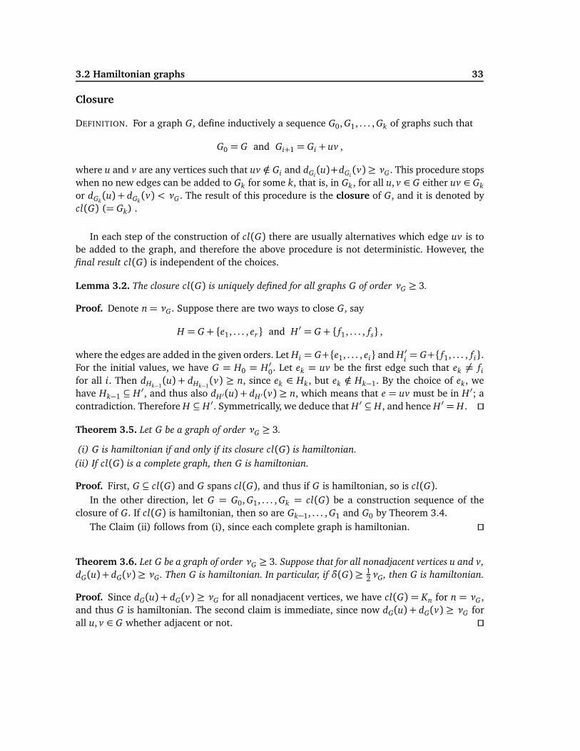
Example 3.4. Consider the Petersen graph on the right, whichappears in many places in graph theory as a counter examplefor various conditions. This graph is not hamiltonian, but it doessatisfy the condition c(G−S) ≤ |S| for all S 6= ;. Therefore theconclusion of Lemma 3.1 is not sufficient to ensure that a graphis hamiltonian.
The following theorem, due to ORE, generalizes an earlier result by DIRAC (1952).
Theorem 3.4 (ORE (1962)). Let G be a graph of order νG ≥ 3, and let u, v ∈ G be such that
dG(u) + dG(v)≥ νG .
Then G is hamiltonian if and only if G + uv is hamiltonian.
Proof. Denote n = νG. Let u, v ∈ G be such that dG(u) + dG(v) ≥ n. If uv ∈ G, then there isnothing to prove. Assume thus that uv /∈ G.
(⇒) This is trivial since if G has a Hamilton cycle C , then C is also a Hamilton cycle of G+uv.(⇐) Denote e = uv and suppose that G + e has a Hamilton cycle C . If C does not use the
edge e, then it is a Hamilton cycle of G. Suppose thus that e is on C . We may then assume thatC : u
⋆−→ v −→ u. Now u = v1 −→ v2 −→ . . . −→ vn = v is a Hamilton path of G. There exists an
i with 1 < i < n such that uvi ∈ G and vi−1v ∈ G. For, otherwise, dG(v) < n − dG(u) wouldcontradict the assumption.
v1 v2 ◦ ◦ vi−1 vi ◦ ◦ vn
But now u= v1⋆−→ vi−1 −→ vn −→ vn−1
⋆−→ vi+1 −→ vi −→ v1 = u is a Hamilton cycle in G. ⊓⊔
3.2 Hamiltonian graphs 33
Closure
DEFINITION. For a graph G, define inductively a sequence G0, G1, . . . , Gk of graphs such that
G0 = G and Gi+1 = Gi + uv ,
where u and v are any vertices such that uv /∈ Gi and dGi(u)+dGi
(v) ≥ νG. This procedure stopswhen no new edges can be added to Gk for some k, that is, in Gk, for all u, v ∈ G either uv ∈ Gk
or dGk(u) + dGk
(v) < νG . The result of this procedure is the closure of G, and it is denoted bycl(G) (= Gk) .
In each step of the construction of cl(G) there are usually alternatives which edge uv is tobe added to the graph, and therefore the above procedure is not deterministic. However, thefinal result cl(G) is independent of the choices.
Lemma 3.2. The closure cl(G) is uniquely defined for all graphs G of order νG ≥ 3.
Proof. Denote n= νG. Suppose there are two ways to close G, say
H = G + {e1, . . . , er} and H ′ = G + { f1, . . . , fs} ,
where the edges are added in the given orders. Let Hi = G+{e1, . . . , ei} and H ′i= G+{ f1, . . . , fi}.
For the initial values, we have G = H0 = H ′0. Let ek = uv be the first edge such that ek 6= fi
for all i. Then dHk−1(u) + dHk−1
(v) ≥ n, since ek ∈ Hk, but ek /∈ Hk−1. By the choice of ek, wehave Hk−1 ⊆ H ′, and thus also dH′(u) + dH′(v) ≥ n, which means that e = uv must be in H ′; acontradiction. Therefore H ⊆ H ′. Symmetrically, we deduce that H ′ ⊆ H, and hence H ′ = H. ⊓⊔
Theorem 3.5. Let G be a graph of order νG ≥ 3.
(i) G is hamiltonian if and only if its closure cl(G) is hamiltonian.
(ii) If cl(G) is a complete graph, then G is hamiltonian.
Proof. First, G ⊆ cl(G) and G spans cl(G), and thus if G is hamiltonian, so is cl(G).In the other direction, let G = G0, G1, . . . , Gk = cl(G) be a construction sequence of the
closure of G. If cl(G) is hamiltonian, then so are Gk−1, . . . , G1 and G0 by Theorem 3.4.The Claim (ii) follows from (i), since each complete graph is hamiltonian. ⊓⊔
Theorem 3.6. Let G be a graph of order νG ≥ 3. Suppose that for all nonadjacent vertices u and v,
dG(u) + dG(v)≥ νG . Then G is hamiltonian. In particular, if δ(G) ≥ 12νG, then G is hamiltonian.
Proof. Since dG(u) + dG(v) ≥ νG for all nonadjacent vertices, we have cl(G) = Kn for n = νG ,and thus G is hamiltonian. The second claim is immediate, since now dG(u) + dG(v) ≥ νG forall u, v ∈ G whether adjacent or not. ⊓⊔
3.2 Hamiltonian graphs 34
Chvátal’s condition
The hamiltonian problem of graphs has attracted much attention, at least partly because theproblem has practical significance. (Indeed, the first example where DNA computing was ap-plied, was the hamiltonian problem.)
There are some general improvements of the previous results of this chapter, and quite manyimprovements in various special cases, where the graphs are somehow restricted. We becomesatisfied by two general results.
Theorem 3.7 (CHVÁTAL (1972)). Let G be a graph with VG = {v1, v2, . . . , vn}, for n ≥ 3, ordered
so that d1 ≤ d2 ≤ · · · ≤ dn, for di = dG(vi). If for every i < n/2,
di ≤ i =⇒ dn−i ≥ n− i , (3.1)
then G is hamiltonian.
Proof. First of all, we may suppose that G is closed, G = cl(G), because G is hamiltonian if andonly if cl(G) is hamiltonian, and adding edges to G does not decrease any of its degrees, thatis, if G satisfies (3.1), so does G + e for every e. We show that, in this case, G = Kn, and thus G
is hamiltonian.Assume on the contrary that G 6= Kn, and let uv /∈ G with dG(u) ≤ dG(v) be such that
dG(u)+ dG(v) is as large as possible. Because G is closed, we must have dG(u)+ dG(v) < n, andtherefore dG(u) = i < n/2. Let A= {w | vw /∈ G, w 6= v}. By our choice, dG(w) ≤ i for all w ∈ A,and, moreover,
|A|= (n− 1)− dG(v)≥ dG(u) = i .
Consequently, there are at least i vertices w with dG(w) ≤ i, and so di ≤ dG(u) = i.Similarly, for each vertex from B = {w | uw /∈ G, w 6= u}, dG(w) ≤ dG(v)< n− dG(u) = n− i,
and|B| = (n− 1)− dG(u) = (n− 1)− i .
Also dG(u) < n− i, and thus there are at least n− i vertices w with dG(w) < n− i. Consequently,dn−i < n− i. This contradicts the obtained bound di ≤ i and the condition (3.1). ⊓⊔
Note that the condition (3.1) is easily checkable for any given graph.
3.3 Matchings 35
3.3 Matchings
In matching problems we are given an availability relation between the elements of a set. Theproblem is then to find a pairing of the elements so that each element is paired (matched)uniquely with an available companion.
A special case of the matching problem is the marriage problem, which is stated as follows.Given a set X of boys and a set Y of girls, under what condition can each boy marry a girl whocares to marry him? This problem has many variations. One of them is the job assignmentproblem, where we are given n applicants and m jobs, and we should assign each applicant toa job he is qualified. The problem is that an applicant may be qualified for several jobs, and ajob may be suited for several applicants.
Maximum matchings
DEFINITION. For a graph G, a subset M ⊆ EG is a matching of G, if M contains no adjacentedges. The two ends of an edge e ∈ M are matched under M . A matching M is a maximummatching, if for no matching M ′, |M | < |M ′|.
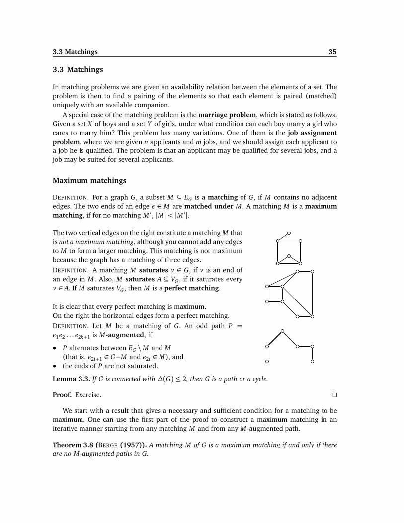
The two vertical edges on the right constitute a matching M thatis not a maximum matching, although you cannot add any edgesto M to form a larger matching. This matching is not maximumbecause the graph has a matching of three edges.
DEFINITION. A matching M saturates v ∈ G, if v is an end ofan edge in M . Also, M saturates A ⊆ VG , if it saturates everyv ∈ A. If M saturates VG , then M is a perfect matching.
It is clear that every perfect matching is maximum.On the right the horizontal edges form a perfect matching.
DEFINITION. Let M be a matching of G. An odd path P =
e1e2 . . . e2k+1 is M -augmented, if
• P alternates between EG \M and M
(that is, e2i+1 ∈ G−M and e2i ∈ M), and• the ends of P are not saturated.
Lemma 3.3. If G is connected with ∆(G) ≤ 2, then G is a path or a cycle.
Proof. Exercise. ⊓⊔
We start with a result that gives a necessary and sufficient condition for a matching to bemaximum. One can use the first part of the proof to construct a maximum matching in aniterative manner starting from any matching M and from any M -augmented path.
Theorem 3.8 (BERGE (1957)). A matching M of G is a maximum matching if and only if there
are no M-augmented paths in G.
3.3 Matchings 36
Proof. (⇒) Let a matching M have an M -augmented path P = e1e2 . . . e2k+1 in G. Heree2, e4, . . . , e2k ∈ M , e1, e3, . . . , e2k+1 /∈ M . Define N ⊆ EG by
N = (M \ {e2i | i ∈ [1, k]}) ∪ {e2i+1 | i ∈ [0, k]} .
Now, N is a matching of G, and |N |= |M |+ 1. Therefore M is not a maximum matching.
(⇐) Assume N is a maximum matching, but M is not. Hence |N | > |M |. Consider the sub-graph H = G[M △N] for the symmetric difference M △N . We have dH(v)≤ 2 for each v ∈ H,because v is an end of at most one edge in M and N . By Lemma 3.3, each connected componentA of H is either a path or a cycle.
Since no v ∈ A can be an end of two edges from N or from M , each connected component(path or a cycle) A alternates between N and M . Now, since |N | > |M |, there is a connectedcomponent A of H, which has more edges from N than from M . This A cannot be a cycle, becausean alternating cycle has even length, and it thus contains equally many edges from N and M .Hence A: u
⋆−→ v is a path (of odd length), which starts and ends with an edge from N . Because
A is a connected component of H, the ends u and v are not saturated by M , and, consequently,A is an M -augmented path. This proves the theorem. ⊓⊔
Example 3.5. Consider the k-cube Qk for k ≥ 1. Each maximum matching of Qk has 2k−1 edges.Indeed, the matching M = {(0u, 1u) | u ∈ Bk−1}, has 2k−1 edges, and it is clearly perfect.
Hall’s theorem
For a subset S ⊆ VG of a graph G, denote
NG(S) = {v | uv ∈ G for some u ∈ S} .
If G is (X , Y )-bipartite, and S ⊆ X , then NG(S) ⊆ Y .
The following result, known as the
Theorem 3.9 (HALL (1935)). Let G be a (X , Y )-bipartite graph. Then G contains a matching M
saturating X if and only if
|S| ≤ |NG(S)| for all S ⊆ X . (3.2)
Proof. (⇒) Let M be a matching that saturates X . If |S|> |NG(S)| for some S ⊆ X , then not allx ∈ S can be matched with different y ∈ NG(S).
(⇐) Let G satisfy Hall’s condition (3.2). We prove the claim by induction on |X |.If |X | = 1, then the claim is clear. Let then |X | ≥ 2, and assume (3.2) implies the existence
of a matching that saturates every proper subset of X .If |NG(S)| ≥ |S| + 1 for every nonempty S ⊆ X with S 6= X , then choose an edge uv ∈ G
with u ∈ X , and consider the induced subgraph H = G−{u, v}. For all S ⊆ X \ {u}, |NH(S)| ≥
|NG(S)| −1≥ |S| , and hence, by the induction hypothesis, H contains a matching M saturatingX \ {u}. Now M ∪ {uv} is a matching saturating X in G, as was required.
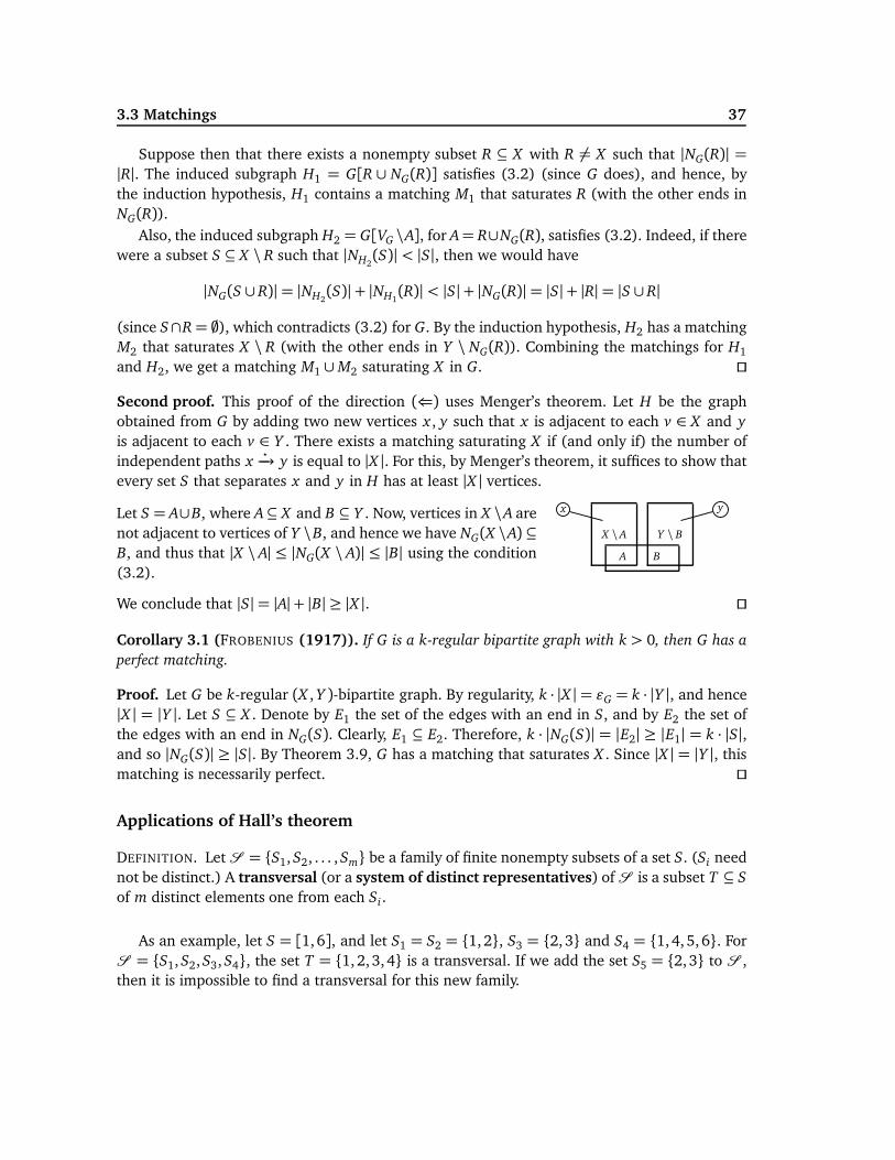
3.3 Matchings 37
Suppose then that there exists a nonempty subset R ⊆ X with R 6= X such that |NG(R)| =
|R|. The induced subgraph H1 = G[R ∪ NG(R)] satisfies (3.2) (since G does), and hence, bythe induction hypothesis, H1 contains a matching M1 that saturates R (with the other ends inNG(R)).
Also, the induced subgraph H2 = G[VG \A], for A= R∪NG(R), satisfies (3.2). Indeed, if therewere a subset S ⊆ X \ R such that |NH2
(S)| < |S|, then we would have
|NG(S ∪ R)| = |NH2(S)|+ |NH1
(R)| < |S|+ |NG(R)| = |S|+ |R|= |S ∪ R|
(since S∩R= ;), which contradicts (3.2) for G. By the induction hypothesis, H2 has a matchingM2 that saturates X \ R (with the other ends in Y \ NG(R)). Combining the matchings for H1
and H2, we get a matching M1 ∪M2 saturating X in G. ⊓⊔
Second proof. This proof of the direction (⇐) uses Menger’s theorem. Let H be the graphobtained from G by adding two new vertices x , y such that x is adjacent to each v ∈ X and y
is adjacent to each v ∈ Y . There exists a matching saturating X if (and only if) the number ofindependent paths x
⋆−→ y is equal to |X |. For this, by Menger’s theorem, it suffices to show that
every set S that separates x and y in H has at least |X | vertices.
Let S = A∪B, where A⊆ X and B ⊆ Y . Now, vertices in X \A arenot adjacent to vertices of Y \B, and hence we have NG(X \A) ⊆
B, and thus that |X \ A| ≤ |NG(X \ A)| ≤ |B| using the condition(3.2).
x y
X \ A Y \ B
A B
We conclude that |S|= |A|+ |B| ≥ |X |. ⊓⊔
Corollary 3.1 (FROBENIUS (1917)). If G is a k-regular bipartite graph with k > 0, then G has a
perfect matching.
Proof. Let G be k-regular (X , Y )-bipartite graph. By regularity, k · |X |= ǫG = k · |Y |, and hence|X | = |Y |. Let S ⊆ X . Denote by E1 the set of the edges with an end in S, and by E2 the set ofthe edges with an end in NG(S). Clearly, E1 ⊆ E2. Therefore, k · |NG(S)| = |E2| ≥ |E1| = k · |S|,and so |NG(S)| ≥ |S|. By Theorem 3.9, G has a matching that saturates X . Since |X | = |Y |, thismatching is necessarily perfect. ⊓⊔
Applications of Hall’s theorem
DEFINITION. Let S = {S1,S2, . . . ,Sm} be a family of finite nonempty subsets of a set S. (Si neednot be distinct.) A transversal (or a system of distinct representatives) of S is a subset T ⊆ S
of m distinct elements one from each Si.
As an example, let S = [1,6], and let S1 = S2 = {1,2}, S3 = {2,3} and S4 = {1,4,5,6}. ForS = {S1,S2,S3,S4}, the set T = {1,2,3,4} is a transversal. If we add the set S5 = {2,3} to S ,then it is impossible to find a transversal for this new family.
3.3 Matchings 38
The connection of transversals to the Marriage Theorem is as follows. Let S = Y and X =
[1, m]. Form an (X , Y )-bipartite graph G such that there is an edge (i, s) if and only if s ∈ Si.The possible transversals T of S are then obtained from the matchings M saturating X in G bytaking the ends in Y of the edges of M .
Corollary 3.2. Let S be a family of finite nonempty sets. Then S has a transversal if and only if
the union of any k of the subsets Si of S contains at least k elements.
Example 3.6. An m× n latin rectangle is an m× n integer matrix M with entries Mi j ∈ [1, n]
such that the entries in the same row and in the same column are different. Moreover, if m = n,then M is a latin square. Note that in a m× n latin rectangle M , we always have that m≤ n.
We show the following: Let M be an m × n latin rectangle (with m < n). Then M can be
extended to a latin square by the addition of n−m new rows.
The claim follows when we show that M can be extended to an (m+ 1)× n latin rectangle.Let Ai ⊆ [1, n] be the set of those elements that do not occur in the i-th column of M . Clearly,|Ai| = n−m for each i, and hence
∑i∈I |Ai|= |I |(n−m) for all subsets I ⊆ [1, n]. Now |∪i∈IAi| ≥
|I |, since otherwise at least one element from the union would be in more than n−m of the setsAi with i ∈ I . However, each row has all the n elements, and therefore each i is missing fromexactly n−m columns. By Marriage Theorem, the family {A1,A2, . . . ,An} has a transversal, andthis transversal can be added as a new row to M . This proves the claim.
Tutte’s theorem
The next theorem is a classic characterization of perfect matchings.
DEFINITION. A connected component of a graph G is said to be odd (even), if it has an odd(even) number of vertices. Denote by codd(G) the number of odd connected components in G.
Denote by m(G) be the number of edges in a maximum matching of a graph G.
Theorem 3.10 (Tutte-Berge Formula). Each maximum matching of a graph G has
m(G) = minS⊆VG
νG + |S| − codd(G−S)
2(3.3)
elements.
Note that the condition in (ii) includes the case, where S = ;.
Proof. We prove the result for connected graphs. The result then follows for disconnectedgraphs by adding the formulas for the connected components.
We observe first that ≤ holds in (3.3), since, for all S ⊆ VG ,
m(G) ≤ |S|+m(G−S) ≤ |S|+|VG \ S| − codd(G−S)
2=νG + |S| − codd(G−S)
2.
3.3 Matchings 39
Indeed, each odd component of G−S must have at least one unsaturated vertex.The proof proceeds by induction on νG . If νG = 1, then the claim is trivial. Suppose that
νG ≥ 2.Assume first that there exists a vertex v ∈ G such that v is saturated by all maximum match-
ings. Then m(G−v) = m(G)− 1. For a subset S′ ⊆ G−v, denote S = S′ ∪ {v}. By the inductionhypothesis, for all S′ ⊆ G−v,
m(G)− 1≥1
2
�(νG − 1) + |S′| − codd(G−(S
′ ∪ {v}))�
=1
2((νG + |S| − codd(G−S)))− 1.
The claim follows from this.Suppose then that for each vertex v, there is a maximum matching that does not saturate v.
We claim that m(G) = (νG −1)/2. Suppose to the contrary, and let M be a maximum matchinghaving two different unsaturated vertices u and v, and choose M so that the distance dG(u, v)
is as small as possible. Now dG(u, v) ≥ 2, since otherwise uv ∈ G could be added to M , con-tradicting the maximality of M . Let w be an intermediate vertex on a shortest path u
⋆−→ v. By
assumption, there exists a maximum matching N that does not saturate w. We can choose N
such that the intersection M ∩N is maximal. Since dG(u, w) < dG(u, v) and dG(w, v) < dG(u, v),N saturates both u and v. The (maximum) matchings N and M leave equally many vertices un-saturated, and hence there exists another vertex x 6= w saturated by M but which is unsaturatedby N . Let e = x y ∈ M . If y is also unsaturated by N , then N ∪ {e} is a matching, contradictingmaximality of N . It also follows that y 6= w. Therefore there exists an edge e′ = yz in N , wherez 6= x . But now N ′ = N ∪ {e} \ {e′} is a maximum matching that does not saturate w. However,N∩M ⊂ N ′∩M contradicts the choice of N . Therefore, every maximum matching leaves exactlyone vertex unsaturated, i.e., m(G) = (νG − 1)/2.
In this case, for S = ;, the right hand side of (3.3) gets value (νG − 1)/2, and hence, by thebeginning of the proof, this must be the minimum of the right hand side. ⊓⊔
For perfect matchings we have the following corollary, since for a perfect matching we havem(G) = (1/2)νG .
Theorem 3.11 (TUTTE (1947)). Let G be a nontrivial graph. The following are equivalent.
(i) G has a perfect matching.
(ii) For every proper subset S ⊂ VG , codd(G−S) ≤ |S|.
Tutte’s theorem does not provide a good algorithm for constructing a perfect matching, be-cause the theorem requires ‘too many cases’. Its applications are mainly in the proofs of otherresults that are related to matchings. There is a good algorithm due to EDMONDS (1965), whichuses ‘blossom shrinkings’, but this algorithm is somewhat involved.
Example 3.7. The simplest connected graph that has no perfect matching is the path P3. Hereremoving the middle vertex creates two odd components.
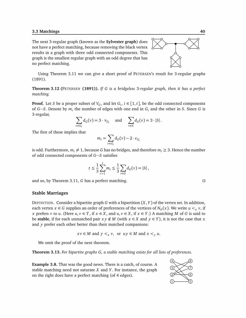
3.3 Matchings 40
The next 3-regular graph (known as the Sylvester graph) doesnot have a perfect matching, because removing the black vertexresults in a graph with three odd connected components. Thisgraph is the smallest regular graph with an odd degree that hasno perfect matching.
Using Theorem 3.11 we can give a short proof of PETERSEN’s result for 3-regular graphs(1891).
Theorem 3.12 (PETERSEN (1891)). If G is a bridgeless 3-regular graph, then it has a perfect
matching.
Proof. Let S be a proper subset of VG , and let Gi , i ∈ [1, t], be the odd connected componentsof G−S. Denote by mi the number of edges with one end in Gi and the other in S. Since G is3-regular, ∑
v∈Gi
dG(v) = 3 · νGiand∑
v∈S
dG(v) = 3 · |S| .
The first of these implies thatmi =∑
v∈Gi
dG(v)− 2 · ǫGi
is odd. Furthermore, mi 6= 1, because G has no bridges, and therefore mi ≥ 3. Hence the numberof odd connected components of G−S satisfies
t ≤1
3
t∑
i=1
mi ≤1
3
∑
v∈S
dG(v) = |S| ,
and so, by Theorem 3.11, G has a perfect matching. ⊓⊔
Stable Marriages
DEFINITION. Consider a bipartite graph G with a bipartition (X , Y ) of the vertex set. In addition,each vertex x ∈ G supplies an order of preferences of the vertices of NG(x). We write u<x v, ifx prefers v to u. (Here u, v ∈ Y , if x ∈ X , and u, v ∈ X , if x ∈ Y .) A matching M of G is said tobe stable, if for each unmatched pair x y /∈ M (with x ∈ X and y ∈ Y ), it is not the case that x
and y prefer each other better than their matched companions:
x v ∈ M and y <x v, or uy ∈ M and x <y u.
We omit the proof of the next theorem.
Theorem 3.13. For bipartite graphs G, a stable matching exists for all lists of preferences.
Example 3.8. That was the good news. There is a catch, of course. Astable matching need not saturate X and Y . For instance, the graphon the right does have a perfect matching (of 4 edges).
4
2
3
1 5
6
7
8
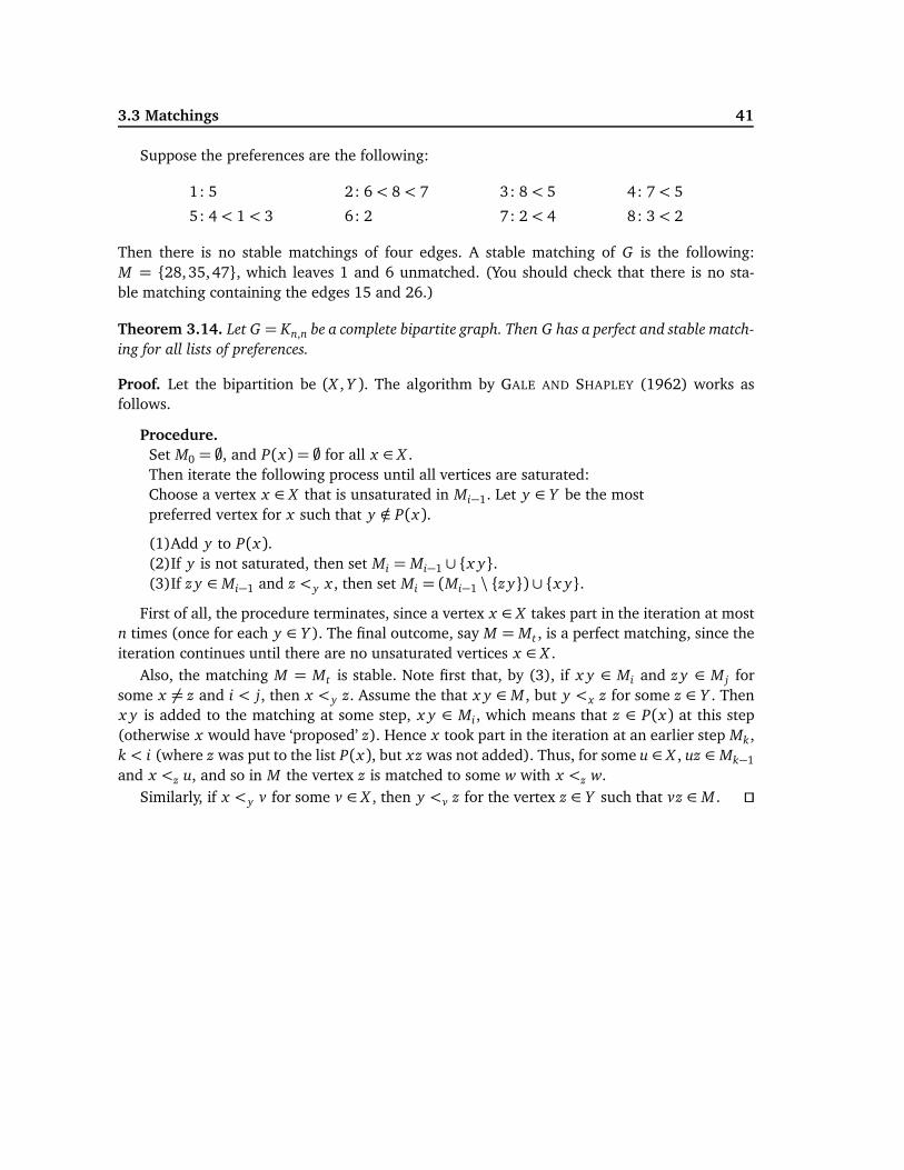
3.3 Matchings 41
Suppose the preferences are the following:
1: 5 2: 6< 8< 7 3: 8< 5 4: 7< 5
5: 4< 1< 3 6: 2 7: 2< 4 8: 3< 2
Then there is no stable matchings of four edges. A stable matching of G is the following:M = {28,35,47}, which leaves 1 and 6 unmatched. (You should check that there is no sta-ble matching containing the edges 15 and 26.)
Theorem 3.14. Let G = Kn,n be a complete bipartite graph. Then G has a perfect and stable match-
ing for all lists of preferences.
Proof. Let the bipartition be (X , Y ). The algorithm by GALE AND SHAPLEY (1962) works asfollows.
Procedure.Set M0 = ;, and P(x) = ; for all x ∈ X .Then iterate the following process until all vertices are saturated:Choose a vertex x ∈ X that is unsaturated in Mi−1. Let y ∈ Y be the mostpreferred vertex for x such that y /∈ P(x).
(1)Add y to P(x).(2)If y is not saturated, then set Mi = Mi−1 ∪ {x y}.(3)If z y ∈ Mi−1 and z <y x , then set Mi = (Mi−1 \ {z y}) ∪ {x y}.
First of all, the procedure terminates, since a vertex x ∈ X takes part in the iteration at mostn times (once for each y ∈ Y ). The final outcome, say M = Mt , is a perfect matching, since theiteration continues until there are no unsaturated vertices x ∈ X .
Also, the matching M = Mt is stable. Note first that, by (3), if x y ∈ Mi and z y ∈ M j forsome x 6= z and i < j, then x <y z. Assume the that x y ∈ M , but y <x z for some z ∈ Y . Thenx y is added to the matching at some step, x y ∈ Mi, which means that z ∈ P(x) at this step(otherwise x would have ‘proposed’ z). Hence x took part in the iteration at an earlier step Mk,k < i (where z was put to the list P(x), but xz was not added). Thus, for some u ∈ X , uz ∈ Mk−1
and x <z u, and so in M the vertex z is matched to some w with x <z w.Similarly, if x <y v for some v ∈ X , then y <v z for the vertex z ∈ Y such that vz ∈ M . ⊓⊔
4
Colourings
4.1 Edge colourings
Colourings of edges and vertices of a graph G are useful, when one is interested in classifyingrelations between objects.
There are two sides of colourings. In the general case, a graph G with a colouring α is given,and we study the properties of this pair Gα = (G,α). This is the situation, e.g., in transportationnetworks with bus and train links, where the colour (buss, train) of an edge tells the nature ofa link.
In the chromatic theory, G is first given and then we search for a colouring that the satisfiesrequired properties. One of the important properties of colourings is ‘properness’. In a propercolouring adjacent edges or vertices are coloured differently.
Edge chromatic number
DEFINITION. A k-edge colouring α: EG → [1, k] of a graph G is an assignment of k colours toits edges. We write Gα to indicate that G has the edge colouring α.
A vertex v ∈ G and a colour i ∈ [1, k] are incident with each other, if α(vu) = i for somevu ∈ G. If v ∈ G is not incident with a colour i, then i is available for v.
The colouring α is proper, if no two adjacent edges obtain the same colour: α(e1) 6= α(e2)
for adjacent e1 and e2.The edge chromatic number χ ′(G) of G is defined as
χ ′(G) =min{k | there exists a proper k-edge colouring of G} .
A k-edge colouring α can be thought of as a partition {E1, E2, . . . , Ek} of EG , where Ei = {e |
α(e) = i}. Note that it is possible that Ei = ; for some i. We adopt a simplified notation
Gα[i1, i2, . . . , it] = G[Ei1∪ Ei2∪ · · · ∪ Eit
]
for the subgraph of G consisting of those edges that have a colour i1, i2, . . . , or it . That is, theedges having other colours are removed.
Lemma 4.1. Each colour set Ei in a proper k-edge colouring is a matching. Moreover, for each
graph G, ∆(G) ≤ χ ′(G) ≤ ǫG.
Proof. This is clear. ⊓⊔
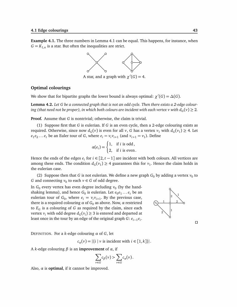
4.1 Edge colourings 43
Example 4.1. The three numbers in Lemma 4.1 can be equal. This happens, for instance, whenG = K1,n is a star. But often the inequalities are strict.
A star, and a graph with χ ′(G) = 4.
Optimal colourings
We show that for bipartite graphs the lower bound is always optimal: χ ′(G) =∆(G).
Lemma 4.2. Let G be a connected graph that is not an odd cycle. Then there exists a 2-edge colour-
ing (that need not be proper), in which both colours are incident with each vertex v with dG(v)≥ 2.
Proof. Assume that G is nontrivial; otherwise, the claim is trivial.
(1) Suppose first that G is eulerian. If G is an even cycle, then a 2-edge colouring exists asrequired. Otherwise, since now dG(v) is even for all v, G has a vertex v1 with dG(v1) ≥ 4. Lete1e2 . . . et be an Euler tour of G, where ei = vi vi+1 (and vt+1 = v1). Define
α(ei) =
¨1, if i is odd ,
2, if i is even .
Hence the ends of the edges ei for i ∈ [2, t − 1] are incident with both colours. All vertices areamong these ends. The condition dG(v1) ≥ 4 guarantees this for v1. Hence the claim holds inthe eulerian case.
(2) Suppose then that G is not eulerian. We define a new graph G0 by adding a vertex v0 toG and connecting v0 to each v ∈ G of odd degree.
In G0 every vertex has even degree including v0 (by the hand-shaking lemma), and hence G0 is eulerian. Let e0e1 . . . et be aneulerian tour of G0, where ei = vi vi+1. By the previous case,there is a required colouring α of G0 as above. Now, α restrictedto EG is a colouring of G as required by the claim, since eachvertex vi with odd degree dG(vi) ≥ 3 is entered and departed atleast once in the tour by an edge of the original graph G: ei−1ei.
v01
21
2
12
⊓⊔
DEFINITION. For a k-edge colouring α of G, let
cα(v) = |{i | v is incident with i ∈ [1, k]}| .
A k-edge colouring β is an improvement of α, if∑
v∈G
cβ (v)>∑
v∈G
cα(v) .
Also, α is optimal, if it cannot be improved.
4.1 Edge colourings 44
Notice that we always have cα(v)≤ dG(v), and if α is proper, then cα(v) = dG(v), and in thiscase α is optimal. Thus an improvement of a colouring is a change towards a proper colouring.Note also that a graph G always has an optimal k-edge colouring, but it need not have anyproper k-edge colourings.
The next lemma is obvious.
Lemma 4.3. An edge colouring α of G is proper if and only if cα(v) = dG(v) for all vertices v ∈ G.
Lemma 4.4. Let α be an optimal k-edge colouring of G, and let v ∈ G. Suppose that the colour i
is available for v, and the colour j is incident with v at least twice. Then the connected component
H of Gα[i, j] that contains v, is an odd cycle.
Proof. Suppose the connected component H is not an odd cycle. By Lemma 4.2, H has a 2-edgecolouring γ: EH → {i, j}, in which both i and j are incident with each vertex x with dH(x)≥ 2.(We have renamed the colours 1 and 2 to i and j.) We obtain a recolouring β of G as follows:
β(e) =
¨γ(e), if e ∈ H ,
α(e), if e /∈ H .
Since dH(v) ≥ 2 (by the assumption on the colour j) and in β both colours i and j are nowincident with v, cβ (v) = cα(v)+1. Furthermore, by the construction of β , we have cβ (u) ≥ cα(u)
for all u 6= v. Therefore∑
u∈G cβ (u) >∑
u∈G cα(u), which contradicts the optimality of α. HenceH is an odd cycle. ⊓⊔
Theorem 4.1 (KÖNIG (1916)). If G is bipartite, then χ ′(G) =∆(G).
Proof. Let α be an optimal ∆-edge colouring of a bipartite G, where ∆ = ∆(G). If there werea v ∈ G with cα(v) < dG(v), then by Lemma 4.4, G would contain an odd cycle. But a bipartitegraph does not contain such cycles. Therefore, for all vertices v, cα(v) = dG(v). By Lemma 4.3,α is a proper colouring, and ∆ = χ ′(G) as required. ⊓⊔
Vizing’s theorem
In general we can have χ ′(G) >∆(G) as one of our examples did show. The following importanttheorem, due to VIZING, shows that the edge chromatic number of a graph G misses ∆(G) byat most one colour.
Theorem 4.2 (VIZING (1964)). For any graph G, ∆(G) ≤ χ ′(G) ≤∆(G) + 1.
Proof. Let ∆ =∆(G). We need only to show that χ ′(G) ≤∆+1. Suppose on the contrary thatχ ′(G) >∆+ 1, and let α be an optimal (∆+ 1)-edge colouring of G.
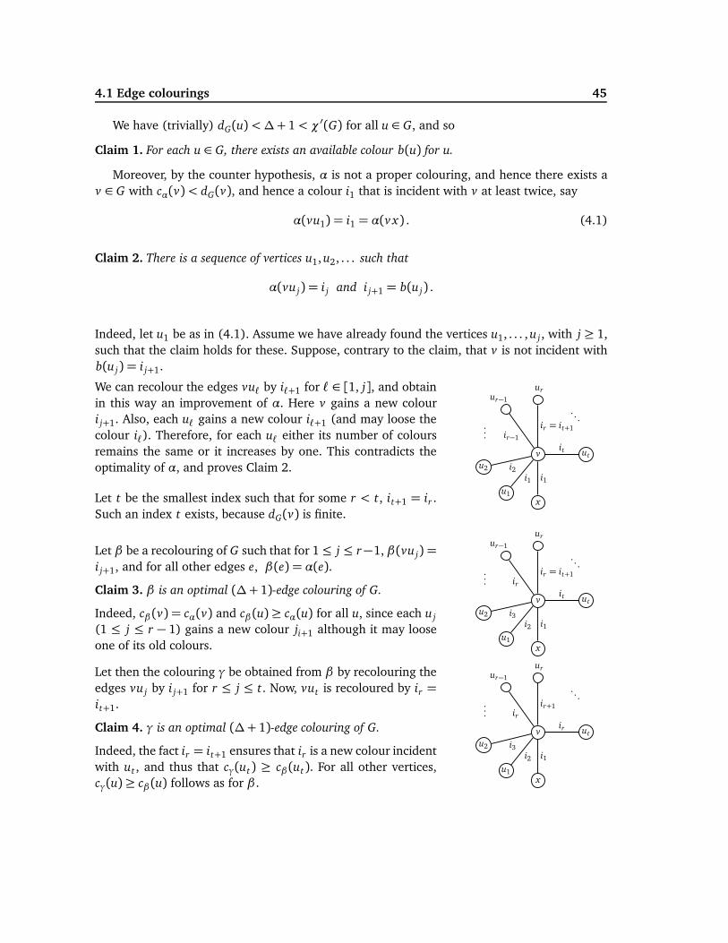
4.1 Edge colourings 45
We have (trivially) dG(u) <∆+ 1< χ ′(G) for all u ∈ G, and so
Claim 1. For each u ∈ G, there exists an available colour b(u) for u.
Moreover, by the counter hypothesis, α is not a proper colouring, and hence there exists av ∈ G with cα(v)< dG(v), and hence a colour i1 that is incident with v at least twice, say
α(vu1) = i1 = α(v x) . (4.1)
Claim 2. There is a sequence of vertices u1,u2, . . . such that
α(vu j) = i j and i j+1 = b(u j) .
Indeed, let u1 be as in (4.1). Assume we have already found the vertices u1, . . . ,u j , with j ≥ 1,such that the claim holds for these. Suppose, contrary to the claim, that v is not incident withb(u j) = i j+1.
We can recolour the edges vuℓ by iℓ+1 for ℓ ∈ [1, j], and obtainin this way an improvement of α. Here v gains a new colouri j+1. Also, each uℓ gains a new colour iℓ+1 (and may loose thecolour iℓ). Therefore, for each uℓ either its number of coloursremains the same or it increases by one. This contradicts theoptimality of α, and proves Claim 2.
Let t be the smallest index such that for some r < t, it+1 = ir .Such an index t exists, because dG(v) is finite.
xu1
u2
ur
v ut
...
.. .
ur−1
i1i1
i2
ir−1
ir = it+1
it
Let β be a recolouring of G such that for 1≤ j ≤ r−1, β(vu j) =
i j+1, and for all other edges e, β(e) = α(e).
Claim 3. β is an optimal (∆+ 1)-edge colouring of G.
Indeed, cβ (v) = cα(v) and cβ (u) ≥ cα(u) for all u, since each u j
(1 ≤ j ≤ r − 1) gains a new colour ji+1 although it may looseone of its old colours. x
u1
u2
ur
v ut
...
.. .
ur−1
i1i2
i3
ir
ir = it+1
it
Let then the colouring γ be obtained from β by recolouring theedges vu j by i j+1 for r ≤ j ≤ t. Now, vut is recoloured by ir =
it+1.
Claim 4. γ is an optimal (∆+ 1)-edge colouring of G.
Indeed, the fact ir = it+1 ensures that ir is a new colour incidentwith ut , and thus that cγ(ut) ≥ cβ (ut). For all other vertices,cγ(u) ≥ cβ (u) follows as for β . x
u1
u2
ur
v ut
...
.. .
ur−1
i1i2
i3
ir
ir+1
ir
4.2 Ramsey Theory 46
By Claim 1, there is a colour i0 = b(v) that is available for v. By Lemma 4.4, the connectedcomponents H1 of Gβ [i0, ir] and H2 of Gγ[i0, ir] containing the vertex v are cycles, that is,H1 is a cycle (vur−1)P1(ur v) and H2 is a cycle (vur−1)P2(ut v), where both P1 : ur−1
⋆−→ ur and
P2 : ur−1⋆−→ ut are paths. However, the edges of P1 and P2 have the same colours with respect
to β and γ (either i0 or ir). This is not possible, since P1 ends in ur while P2 ends in a differentvertex ut . This contradiction proves the theorem. ⊓⊔
Example 4.2. We show that χ ′(G) = 4 for the Petersen graph. Indeed, by Vizing’ theorem,χ ′(G) = 3 or 4. Suppose 3 colours suffice. Let C : v1 −→ . . . −→ v5 −→ v1 be the outer cycle andC ′ : u1 −→ . . . −→ u5 −→ u1 the inner cycle of G such that viui ∈ EG for all i.
Observe that every vertex is adjacent to all colours 1,2,3. Now C uses one colour (say 1)once and the other two twice. This can be done uniquely (up to permutations):
v11−→ v2
2−→ v3
3−→ v4
2−→ v5
3−→ v1.
Hence v12−→ u1, v2
3−→ u2, v3
1−→ u3, v4
1−→ u4, v5
1−→ u5. However, this means that 1 cannot be a
colour of any edge in C ′. Since C ′ needs three colours, the claim follows.
Edge Colouring Problem. Vizing’s theorem (nor its present proof) does not offer any charac-terization for the graphs, for which χ ′(G) = ∆(G) + 1. In fact, it is one of the famous openproblems of graph theory to find such a characterization. The answer is known (only) for somespecial classes of graphs. By HOLYER (1981), the problem whether χ ′(G) is ∆(G) or ∆(G) + 1is NP-complete.
The proof of Vizing’s theorem can be used to obtain a proper colouring of G with at most∆(G) + 1 colours, when the word ‘optimal’ is forgotten: colour first the edges as well as youcan (if nothing better, then arbitrarily in two colours), and use the proof iteratively to improvethe colouring until no improvement is possible – then the proof says that the result is a propercolouring.
4.2 Ramsey Theory
In general, Ramsey theory studies unavoidable patterns in combinatorics. We consider an in-stance of this theory mainly for edge colourings (that need not be proper). A typical exampleof a Ramsey property is the following: given 6 persons each pair of whom are either friends orenemies, there are then 3 persons who are mutual friends or mutual enemies. In graph theoreticterms this means that each colouring of the edges of K6 with 2 colours results in a monochro-matic triangle.
Turan’s theorem for complete graphs
We shall first consider the problem of finding a general condition for Kp to appear in a graph.It is clear that every graph contains K1, and that every nondiscrete graph contains K2.
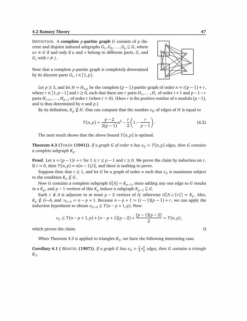
4.2 Ramsey Theory 47
DEFINITION. A complete p-partite graph G consists of p dis-crete and disjoint induced subgraphs G1, G2, . . . , Gp ⊆ G, whereuv ∈ G if and only if u and v belong to different parts, Gi andG j with i 6= j.
Note that a complete p-partite graph is completely determinedby its discrete parts Gi, i ∈ [1, p].
Let p ≥ 3, and let H = Hn,p be the complete (p− 1)-partite graph of order n= t(p − 1) + r,where r ∈ [1, p−1] and t ≥ 0, such that there are r parts H1, . . . , Hr of order t+1 and p−1− r
parts Hr+1, . . . , Hp−1 of order t (when t > 0). (Here r is the positive residue of n modulo (p−1),and is thus determined by n and p.)
By its definition, Kp * H. One can compute that the number ǫH of edges of H is equal to
T (n, p) =p− 2
2(p− 1)n2 −
r
2
�1−
r
p− 1
�. (4.2)
The next result shows that the above bound T (n, p) is optimal.
Theorem 4.3 (TURÁN (1941)). If a graph G of order n has ǫG > T (n, p) edges, then G contains
a complete subgraph Kp.
Proof. Let n = (p− 1)t + r for 1≤ r ≤ p− 1 and t ≥ 0. We prove the claim by induction on t.If t = 0, then T (n, p) = n(n− 1)/2, and there is nothing to prove.
Suppose then that t ≥ 1, and let G be a graph of order n such that ǫG is maximum subjectto the condition Kp * G.
Now G contains a complete subgraph G[A] = Kp−1, since adding any one edge to G resultsin a Kp, and p− 1 vertices of this Kp induce a subgraph Kp−1 ⊆ G.
Each v /∈ A is adjacent to at most p − 2 vertices of A; otherwise G[A ∪ {v}] = Kp. Also,Kp * G−A, and νG−A = n − p + 1. Because n − p + 1 = (t − 1)(p − 1) + r, we can apply theinduction hypothesis to obtain ǫG−A ≤ T (n− p+ 1, p). Now
ǫG ≤ T (n− p+ 1, p) + (n− p+ 1)(p− 2) +(p − 1)(p− 2)
2= T (n, p) ,
which proves the claim. ⊓⊔
When Theorem 4.3 is applied to triangles K3, we have the following interesting case.
Corollary 4.1 ( MANTEL (1907)). If a graph G has ǫG >14ν
2G
edges, then G contains a triangle
K3.
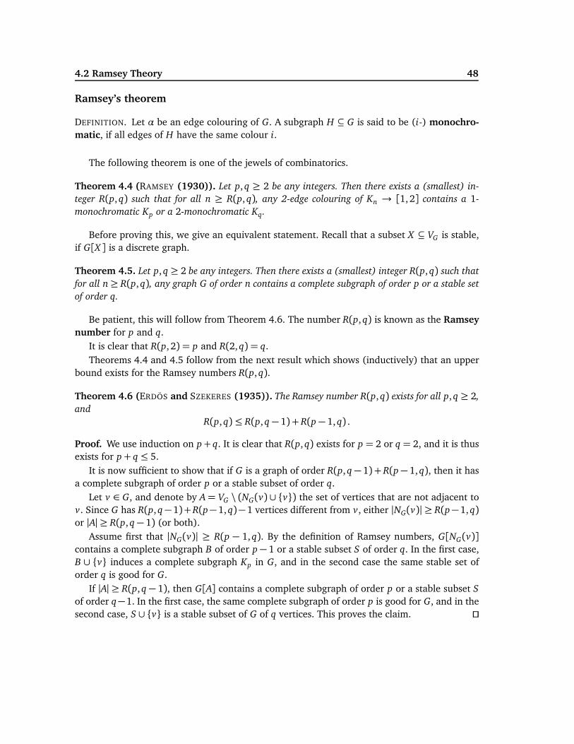
4.2 Ramsey Theory 48
Ramsey’s theorem
DEFINITION. Let α be an edge colouring of G. A subgraph H ⊆ G is said to be (i-) monochro-matic, if all edges of H have the same colour i.
The following theorem is one of the jewels of combinatorics.
Theorem 4.4 (RAMSEY (1930)). Let p,q ≥ 2 be any integers. Then there exists a (smallest) in-
teger R(p,q) such that for all n ≥ R(p,q), any 2-edge colouring of Kn → [1,2] contains a 1-
monochromatic Kp or a 2-monochromatic Kq.
Before proving this, we give an equivalent statement. Recall that a subset X ⊆ VG is stable,if G[X ] is a discrete graph.
Theorem 4.5. Let p,q ≥ 2 be any integers. Then there exists a (smallest) integer R(p,q) such that
for all n≥ R(p,q), any graph G of order n contains a complete subgraph of order p or a stable set
of order q.
Be patient, this will follow from Theorem 4.6. The number R(p,q) is known as the Ramseynumber for p and q.
It is clear that R(p, 2) = p and R(2,q) = q.Theorems 4.4 and 4.5 follow from the next result which shows (inductively) that an upper
bound exists for the Ramsey numbers R(p,q).
Theorem 4.6 (ERDÖS and SZEKERES (1935)). The Ramsey number R(p,q) exists for all p,q ≥ 2,
and
R(p,q) ≤ R(p,q − 1) + R(p− 1,q) .
Proof. We use induction on p+ q. It is clear that R(p,q) exists for p = 2 or q = 2, and it is thusexists for p+ q ≤ 5.
It is now sufficient to show that if G is a graph of order R(p,q − 1) + R(p− 1,q), then it hasa complete subgraph of order p or a stable subset of order q.
Let v ∈ G, and denote by A= VG \ (NG(v) ∪ {v}) the set of vertices that are not adjacent tov. Since G has R(p,q−1)+R(p−1,q)−1 vertices different from v, either |NG(v)| ≥ R(p−1,q)or |A| ≥ R(p,q − 1) (or both).
Assume first that |NG(v)| ≥ R(p − 1,q). By the definition of Ramsey numbers, G[NG(v)]
contains a complete subgraph B of order p− 1 or a stable subset S of order q. In the first case,B ∪ {v} induces a complete subgraph Kp in G, and in the second case the same stable set oforder q is good for G.
If |A| ≥ R(p,q − 1), then G[A] contains a complete subgraph of order p or a stable subset S
of order q−1. In the first case, the same complete subgraph of order p is good for G, and in thesecond case, S ∪ {v} is a stable subset of G of q vertices. This proves the claim. ⊓⊔
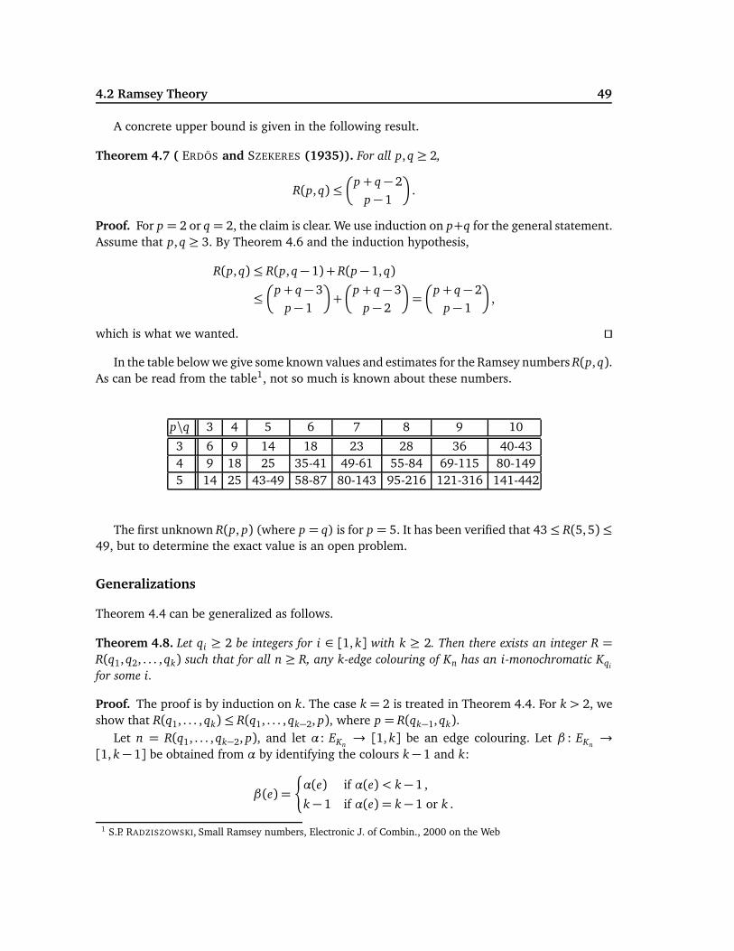
4.2 Ramsey Theory 49
A concrete upper bound is given in the following result.
Theorem 4.7 ( ERDÖS and SZEKERES (1935)). For all p,q ≥ 2,
R(p,q) ≤�
p+ q− 2
p− 1
�.
Proof. For p = 2 or q = 2, the claim is clear. We use induction on p+q for the general statement.Assume that p,q ≥ 3. By Theorem 4.6 and the induction hypothesis,
R(p,q) ≤ R(p,q− 1) + R(p− 1,q)
≤
�p+ q− 3
p− 1
�+
�p+ q− 3
p− 2
�=
�p+ q− 2
p− 1
�,
which is what we wanted. ⊓⊔
In the table below we give some known values and estimates for the Ramsey numbers R(p,q).As can be read from the table1, not so much is known about these numbers.
p\q 3 4 5 6 7 8 9 10
3 6 9 14 18 23 28 36 40-434 9 18 25 35-41 49-61 55-84 69-115 80-1495 14 25 43-49 58-87 80-143 95-216 121-316 141-442
The first unknown R(p, p) (where p = q) is for p = 5. It has been verified that 43≤ R(5,5)≤49, but to determine the exact value is an open problem.
Generalizations
Theorem 4.4 can be generalized as follows.
Theorem 4.8. Let qi ≥ 2 be integers for i ∈ [1, k] with k ≥ 2. Then there exists an integer R =
R(q1,q2, . . . ,qk) such that for all n ≥ R, any k-edge colouring of Kn has an i-monochromatic Kqi
for some i.
Proof. The proof is by induction on k. The case k = 2 is treated in Theorem 4.4. For k > 2, weshow that R(q1, . . . ,qk) ≤ R(q1, . . . ,qk−2, p), where p = R(qk−1,qk).
Let n = R(q1, . . . ,qk−2, p), and let α: EKn→ [1, k] be an edge colouring. Let β : EKn
→
[1, k − 1] be obtained from α by identifying the colours k− 1 and k:
β(e) =
¨α(e) if α(e) < k− 1 ,
k − 1 if α(e) = k− 1 or k .
1 S.P. RADZISZOWSKI, Small Ramsey numbers, Electronic J. of Combin., 2000 on the Web
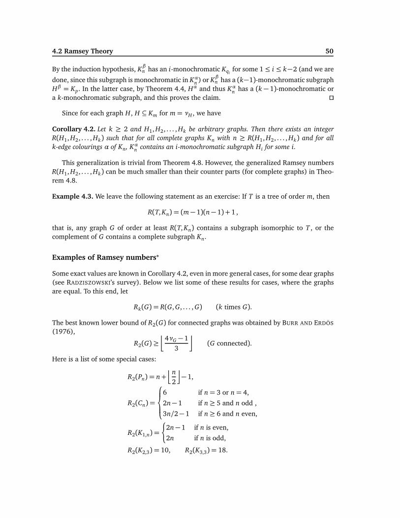
4.2 Ramsey Theory 50
By the induction hypothesis, Kβn has an i-monochromatic Kqi
for some 1≤ i ≤ k−2 (and we are
done, since this subgraph is monochromatic in Kαn ) or Kβn has a (k−1)-monochromatic subgraph
Hβ = Kp. In the latter case, by Theorem 4.4, Hα and thus Kαn has a (k − 1)-monochromatic ora k-monochromatic subgraph, and this proves the claim. ⊓⊔
Since for each graph H, H ⊆ Km for m= νH , we have
Corollary 4.2. Let k ≥ 2 and H1, H2, . . . , Hk be arbitrary graphs. Then there exists an integer
R(H1, H2, . . . , Hk) such that for all complete graphs Kn with n ≥ R(H1, H2, . . . , Hk) and for all
k-edge colourings α of Kn, Kαn contains an i-monochromatic subgraph Hi for some i.
This generalization is trivial from Theorem 4.8. However, the generalized Ramsey numbersR(H1, H2, . . . , Hk) can be much smaller than their counter parts (for complete graphs) in Theo-rem 4.8.
Example 4.3. We leave the following statement as an exercise: If T is a tree of order m, then
R(T, Kn) = (m− 1)(n− 1) + 1 ,
that is, any graph G of order at least R(T, Kn) contains a subgraph isomorphic to T , or thecomplement of G contains a complete subgraph Kn.
Examples of Ramsey numbers∗
Some exact values are known in Corollary 4.2, even in more general cases, for some dear graphs(see RADZISZOWSKI’s survey). Below we list some of these results for cases, where the graphsare equal. To this end, let
Rk(G) = R(G, G, . . . , G) (k times G).
The best known lower bound of R2(G) for connected graphs was obtained by BURR AND ERDÖS
(1976),
R2(G) ≥
�4νG − 1
3
�(G connected).
Here is a list of some special cases:
R2(Pn) = n+
jn
2
k− 1,
R2(Cn) =
6 if n= 3 or n= 4,
2n− 1 if n≥ 5 and n odd ,
3n/2− 1 if n≥ 6 and n even,
R2(K1,n) =
¨2n− 1 if n is even,
2n if n is odd,
R2(K2,3) = 10, R2(K3,3) = 18.
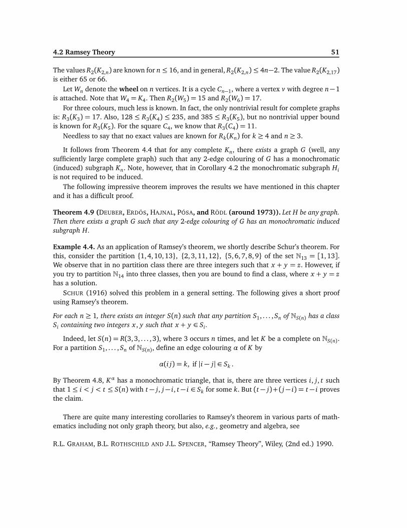
4.2 Ramsey Theory 51
The values R2(K2,n) are known for n≤ 16, and in general, R2(K2,n)≤ 4n−2. The value R2(K2,17)
is either 65 or 66.Let Wn denote the wheel on n vertices. It is a cycle Cn−1, where a vertex v with degree n−1
is attached. Note that W4 = K4. Then R2(W5) = 15 and R2(W6) = 17.For three colours, much less is known. In fact, the only nontrivial result for complete graphs
is: R3(K3) = 17. Also, 128 ≤ R3(K4) ≤ 235, and 385 ≤ R3(K5), but no nontrivial upper boundis known for R3(K5). For the square C4, we know that R3(C4) = 11.
Needless to say that no exact values are known for Rk(Kn) for k ≥ 4 and n≥ 3.
It follows from Theorem 4.4 that for any complete Kn, there exists a graph G (well, anysufficiently large complete graph) such that any 2-edge colouring of G has a monochromatic(induced) subgraph Kn. Note, however, that in Corollary 4.2 the monochromatic subgraph Hi
is not required to be induced.The following impressive theorem improves the results we have mentioned in this chapter
and it has a difficult proof.
Theorem 4.9 (DEUBER, ERDÖS, HAJNAL, PÓSA, and RÖDL (around 1973)). Let H be any graph.
Then there exists a graph G such that any 2-edge colouring of G has an monochromatic induced
subgraph H.
Example 4.4. As an application of Ramsey’s theorem, we shortly describe Schur’s theorem. Forthis, consider the partition {1,4,10,13}, {2,3,11,12}, {5,6,7,8,9} of the set N13 = [1,13].We observe that in no partition class there are three integers such that x + y = z. However, ifyou try to partition N14 into three classes, then you are bound to find a class, where x + y = z
has a solution.SCHUR (1916) solved this problem in a general setting. The following gives a short proof
using Ramsey’s theorem.
For each n ≥ 1, there exists an integer S(n) such that any partition S1, . . . ,Sn of NS(n) has a class
Si containing two integers x , y such that x + y ∈ Si .
Indeed, let S(n) = R(3,3, . . . , 3), where 3 occurs n times, and let K be a complete on NS(n).For a partition S1, . . . ,Sn of NS(n), define an edge colouring α of K by
α(i j) = k, if |i − j| ∈ Sk .
By Theorem 4.8, Kα has a monochromatic triangle, that is, there are three vertices i, j, t suchthat 1≤ i < j < t ≤ S(n) with t− j, j− i, t− i ∈ Sk for some k. But (t− j)+( j− i) = t− i provesthe claim.
There are quite many interesting corollaries to Ramsey’s theorem in various parts of math-ematics including not only graph theory, but also, e.g., geometry and algebra, see
R.L. GRAHAM, B.L. ROTHSCHILD AND J.L. SPENCER, “Ramsey Theory”, Wiley, (2nd ed.) 1990.
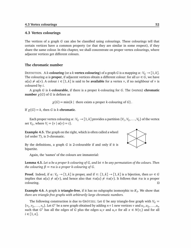
4.3 Vertex colourings 52
4.3 Vertex colourings
The vertices of a graph G can also be classified using colourings. These colourings tell thatcertain vertices have a common property (or that they are similar in some respect), if theyshare the same colour. In this chapter, we shall concentrate on proper vertex colourings, whereadjacent vertices get different colours.
The chromatic number
DEFINITION. A k-colouring (or a k-vertex colouring) of a graph G is a mapping α: VG → [1, k].The colouring α is proper, if adjacent vertices obtain a different colour: for all uv ∈ G, we haveα(u) 6= α(v). A colour i ∈ [1, k] is said to be available for a vertex v, if no neighbour of v iscoloured by i.
A graph G is k-colourable, if there is a proper k-colouring for G. The (vertex) chromaticnumber χ(G) of G is defines as
χ(G) =min{k | there exists a proper k-colouring of G} .
If χ(G) = k, then G is k-chromatic.
Each proper vertex colouring α: VG → [1, k] provides a partition {V1, V2, . . . , Vk} of the vertexset VG , where Vi = {v | α(v) = i}.
Example 4.5. The graph on the right, which is often called a wheel(of order 7), is 3-chromatic.
By the definitions, a graph G is 2-colourable if and only if it isbipartite.
Again, the ‘names’ of the colours are immaterial:
Lemma 4.5. Let α be a proper k-colouring of G, and let π be any permutation of the colours. Then
the colouring β = πα is a proper k-colouring of G.
Proof. Indeed, if α: VG → [1, k] is proper, and if π: [1, k]→ [1, k] is a bijection, then uv ∈ G
implies that α(u) 6= α(v), and hence also that πα(u) 6= πα(v). It follows that πα is a propercolouring. ⊓⊔
Example 4.6. A graph is triangle-free, if it has no subgraphs isomorphic to K3. We show thatthere are triangle-free graphs with arbitrarily large chromatic numbers.
The following construction is due to GRÖTZEL: Let G be any triangle-free graph with VG =
{v1, v2, . . . , vn}. Let G t be a new graph obtained by adding n+1 new vertices v and u1,u2, . . . ,un
such that G t has all the edges of G plus the edges ui v and ui x for all x ∈ N (vi) and for alli ∈ [1, n].
4.3 Vertex colourings 53
Claim. G t is triangle-free and it is k + 1-chromaticIndeed, let U = {u1, . . . ,un}. We show first that G t is triangle-free. Now, U is stable, and so a
triangle contains at most (and thus exactly) one vertex ui ∈ U . If {ui, v j , vk} induces a triangle,so does {vi, v j , vk} by the definition of G t , but the latter triangle is already in G; a contradiction.
For the chromatic number we notice first that χ(G t) ≤ (k + 1). If α is a proper k-colouringof G, extend it by setting α(ui) = α(vi) and α(v) = k+ 1.
Secondly, χ(G t) > k. Assume that α is a proper k-colouring of G t , say with α(v) = k. Thenα(ui) 6= k. Recolour each vi by α(ui). This gives a proper (k−1)-colouring to G; a contradiction.Therefore χ(G t ) = k + 1.
Now using inductively the above construction starting from the triangle-free graph K2, weobtain larger triangle -free graphs with high chromatic numbers.
Critical graphs
DEFINITION. A k-chromatic graph G is said to be k-critical, if χ(H) < k for all H ⊆ G withH 6= G.
In a critical graph an elimination of any edge and of any vertex will reduce the chromaticnumber: χ(G−e) < χ(G) and χ(G−v) < χ(G) for e ∈ G and v ∈ G. Each Kn is n-critical, sincein Kn−(uv) the vertices u and v can gain the same colour.
Example 4.7. The graph K2 = P2 is the only 2-critical graph. The 3-critical graphs are exactlythe odd cycles C2n+1 for n ≥ 1, since a 3-chromatic G is not bipartite, and thus must have acycle of odd length.
Theorem 4.10. If G is k-critical for k ≥ 2, then it is connected, and δ(G) ≥ k− 1.
Proof. Note that for any graph G with the connected components G1, G2, . . . , Gm, χ(G) =max{χ(Gi) | i ∈ [1, m]} . Connectivity claim follows from this observation.
Let then G be k-critical, but δ(G) = dG(v) ≤ k − 2 for v ∈ G. Since G is critical, there is aproper (k−1)-colouring of G−v. Now v is adjacent to only δ(G) < k−1 vertices. But there arek colours, and hence there is an available colour i for v. If we recolour v by i, then a proper(k − 1)-colouring is obtained for G; a contradiction. ⊓⊔
The case (iii) of the next theorem is due to SZEKERES AND WILF (1968).
Theorem 4.11. Let G be any graph with k = χ(G).
(i) G has a k-critical subgraph H.
(ii) G has at least k vertices of degree ≥ k − 1.
(iii) k ≤ 1+maxH⊆G δ(H).
Proof. For (i), we observe that a k-critical subgraph H ⊆ G is obtained by removing verticesand edges from G as long as the chromatic number remains k.
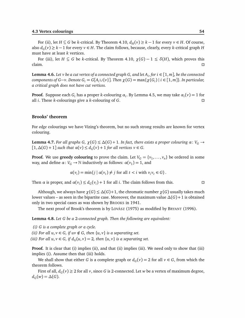
4.3 Vertex colourings 54
For (ii), let H ⊆ G be k-critical. By Theorem 4.10, dH(v)≥ k− 1 for every v ∈ H. Of course,also dG(v)≥ k−1 for every v ∈ H. The claim follows, because, clearly, every k-critical graph H
must have at least k vertices.For (iii), let H ⊆ G be k-critical. By Theorem 4.10, χ(G) − 1 ≤ δ(H), which proves this
claim. ⊓⊔
Lemma 4.6. Let v be a cut vertex of a connected graph G, and let Ai , for i ∈ [1, m], be the connected
components of G−v. Denote Gi = G[Ai∪{v}]. Then χ(G) =max{χ(Gi) | i ∈ [1, m]}. In particular,
a critical graph does not have cut vertices.
Proof. Suppose each Gi has a proper k-colouring αi. By Lemma 4.5, we may take αi(v) = 1 forall i. These k-colourings give a k-colouring of G. ⊓⊔
Brooks’ theorem
For edge colourings we have Vizing’s theorem, but no such strong results are known for vertexcolouring.
Lemma 4.7. For all graphs G, χ(G) ≤∆(G) + 1. In fact, there exists a proper colouring α: VG →
[1,∆(G) + 1] such that α(v)≤ dG(v) + 1 for all vertices v ∈ G.
Proof. We use greedy colouring to prove the claim. Let VG = {v1, . . . , vn} be ordered in someway, and define α: VG → N inductively as follows: α(v1) = 1, and
α(vi) =min{ j | α(vt) 6= j for all t < i with vi vt ∈ G} .
Then α is proper, and α(vi) ≤ dG(vi) + 1 for all i. The claim follows from this. ⊓⊔
Although, we always have χ(G) ≤∆(G)+1, the chromatic number χ(G) usually takes muchlower values – as seen in the bipartite case. Moreover, the maximum value∆(G)+1 is obtainedonly in two special cases as was shown by BROOKS in 1941.
The next proof of Brook’s theorem is by LOVÁSZ (1975) as modified by BRYANT (1996).
Lemma 4.8. Let G be a 2-connected graph. Then the following are equivalent:
(i) G is a complete graph or a cycle.
(ii) For all u, v ∈ G, if uv /∈ G, then {u, v} is a separating set.
(iii) For all u, v ∈ G, if dG(u, v) = 2, then {u, v} is a separating set.
Proof. It is clear that (i) implies (ii), and that (ii) implies (iii). We need only to show that (iii)implies (i). Assume then that (iii) holds.
We shall show that either G is a complete graph or dG(v) = 2 for all v ∈ G, from which thetheorem follows.
First of all, dG(v) ≥ 2 for all v, since G is 2-connected. Let w be a vertex of maximum degree,dG(w) =∆(G).
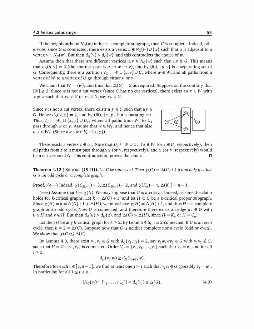
4.3 Vertex colourings 55
If the neighbourhood NG(w) induces a complete subgraph, then G is complete. Indeed, oth-erwise, since G is connected, there exists a vertex u /∈ NG(w) ∪ {w} such that u is adjacent to avertex v ∈ NG(w). But then dG(v) > dG(w), and this contradicts the choice of w.
Assume then that there are different vertices u, v ∈ NG(w) such that uv /∈ G. This meansthat dG(u, v) = 2 (the shortest path is u −→ w −→ v), and by (iii), {u, v} is a separating set ofG. Consequently, there is a partition VG = W ∪ {u, v} ∪ U , where w ∈ W , and all paths from avertex of W to a vertex of U go through either u or v.
We claim that W = {w}, and thus that ∆(G) = 2 as required. Suppose on the contrary that|W | ≥ 2. Since w is not a cut vertex (since G has no cut vertices), there exists an x ∈ W withx 6= w such that xu ∈ G or x v ∈ G, say xu ∈ G.
Since v is not a cut vertex, there exists a y ∈ U such that uy ∈
G. Hence dG(x , y) = 2, and by (iii), {x , y} is a separating set.Thus VG = W1 ∪ {x , y} ∪ U1, where all paths from W1 to U1
pass through x or y. Assume that w ∈W1, and hence that alsou, v ∈W1. (Since uw, vw ∈ VG−{x , y}).
w x
u
v
y
There exists a vertex z ∈ U1. Note that U1 ⊆W ∪ U . If z ∈W (or z ∈ U , respectively), thenall paths from z to u must pass through x (or y, respectively), and x (or y, respectively) wouldbe a cut vertex of G. This contradiction, proves the claim. ⊓⊔
Theorem 4.12 ( BROOKS (1941)). Let G be connected. Then χ(G) =∆(G)+1 if and only if either
G is an odd cycle or a complete graph.
Proof. (⇐=) Indeed, χ(C2k+1) = 3, ∆(C2k+1) = 2, and χ(Kn) = n, ∆(Kn) = n− 1.
(=⇒) Assume that k = χ(G). We may suppose that G is k-critical. Indeed, assume the claimholds for k-critical graphs. Let k = ∆(G) + 1, and let H ⊂ G be a k-critical proper subgraph.Since χ(H) = k =∆(G)+1 >∆(H), we must have χ(H) =∆(H)+1, and thus H is a completegraph or an odd cycle. Now G is connected, and therefore there exists an edge uv ∈ G withu ∈ H and v /∈ H. But then dG(u) > dH(u), and ∆(G) >∆(H), since H = Kn or H = Cn.
Let then G be any k-critical graph for k ≥ 2. By Lemma 4.6, it is 2-connected. If G is an even
cycle, then k = 2 = ∆(G). Suppose now that G is neither complete nor a cycle (odd or even).We show that χ(G) ≤∆(G).
By Lemma 4.8, there exist v1, v2 ∈ G with dG(v1, v2) = 2, say v1w, wv2 ∈ G with v1v2 /∈ G,such that H = G−{v1, v2} is connected. Order VH = {v3, v4, . . . , vn} such that vn = w, and for alli ≥ 3,
dH(vi , w) ≥ dH(vi+1, w) .
Therefore for each i ∈ [1, n−1], we find at least one j > i such that vi v j ∈ G (possibly v j = w).In particular, for all 1≤ i < n,
|NG(vi)∩ {v1, . . . , vi−1}| < dG(vi) ≤∆(G) . (4.3)
4.3 Vertex colourings 56
Then colour v1, v2, . . . , vn in this order as follows: α(v1) = 1= α(v2) and
α(vi) =min{r | r 6= α(v j) for all v j ∈ NG(vi) with j < i} .
The colouring α is proper.By (4.3), α(vi) ≤∆(G) for all i ∈ [1, n− 1]. Also, w = vn has two neighbours, v1 and v2, of
the same colour 1, and since vn has at most ∆(G) neighbours, there is an available colour forvn, and so α(vn) ≤ ∆(G). This shows that G has a proper ∆(G)-colouring, and, consequently,χ(G) ≤∆(G). ⊓⊔
Example 4.8. Suppose we have n objects V = {v1, . . . , vn}, some of which are not compatible(like chemicals that react with each other, or worse, graph theorists who will fight during aconference). In the storage problem we would like to find a partition of the set V with as fewclasses as possible such that no class contains two incompatible elements. In graph theoreticalterminology we consider the graph G = (V, E), where vi v j ∈ E just in case vi and v j are incom-patible, and we would like to colour the vertices of G properly using as few colours as possible.This problem requires that we find χ(G).
Unfortunately, no good algorithms are known for determining χ(G), and, indeed, the chro-matic number problem is NP-complete. Already the problem if χ(G) = 3 is NP-complete. (How-ever, as we have seen, the problem whether χ(G) = 2 has a fast algorithm.)
The chromatic polynomial
A given graph G has many different proper vertex colourings α: VG → [1, k] for sufficientlylarge natural numbers k. Indeed, see Lemma 4.5 to be certain on this point.
DEFINITION. The chromatic polynomial of G is the function χG : N→ N, where
χG(k) = |{α | α: VG → [1, k] a proper colouring}| .
This notion was introduced by BIRKHOFF (1912), BIRKHOFF AND LEWIS (1946), to attack thefamous 4-Colour Theorem, but its applications have turned out to be elsewhere.
If k < χ(G), then clearly χG(k) = 0, and, indeed,
χ(G) =min{k | χG(k) 6= 0} .
Therefore, if we can find the chromatic polynomial of G, then we easily compute the chro-matic number χ(G) just by evaluating χG(k) for k = 1,2, . . . until we hit a nonzero value.Theorem 4.13 will give the tools for constructing χG.
Example 4.9. Consider the complete graph K4 on {v1, v2, v3, v4}. Let k ≥ χ(K4) = 4. The vertexv1 can be first given any of the k colours, after which k−1 colours are available for v2. Then v3
has k − 2 and finally v4 has k − 3 available colours. Therefore there are k(k − 1)(k − 2)(k − 3)different ways to properly colour K4 with k colours, and so
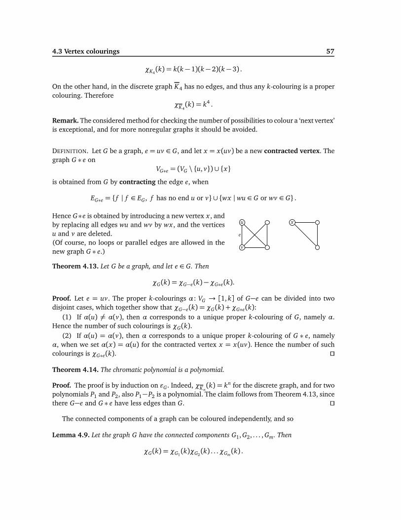
4.3 Vertex colourings 57
χK4(k) = k(k − 1)(k− 2)(k − 3) .
On the other hand, in the discrete graph K4 has no edges, and thus any k-colouring is a propercolouring. Therefore
χK4(k) = k4 .
Remark. The considered method for checking the number of possibilities to colour a ‘next vertex’is exceptional, and for more nonregular graphs it should be avoided.
DEFINITION. Let G be a graph, e = uv ∈ G, and let x = x(uv) be a new contracted vertex. Thegraph G ∗ e on
VG∗e = (VG \ {u, v}) ∪ {x}
is obtained from G by contracting the edge e, when
EG∗e = { f | f ∈ EG, f has no end u or v} ∪ {wx | wu ∈ G or wv ∈ G} .
Hence G∗e is obtained by introducing a new vertex x , andby replacing all edges wu and wv by wx , and the verticesu and v are deleted.(Of course, no loops or parallel edges are allowed in thenew graph G ∗ e.)
v
u x
e
Theorem 4.13. Let G be a graph, and let e ∈ G. Then
χG(k) = χG−e(k)−χG∗e(k).
Proof. Let e = uv. The proper k-colourings α: VG → [1, k] of G−e can be divided into twodisjoint cases, which together show that χG−e(k) = χG(k) +χG∗e(k):
(1) If α(u) 6= α(v), then α corresponds to a unique proper k-colouring of G, namely α.Hence the number of such colourings is χG(k).
(2) If α(u) = α(v), then α corresponds to a unique proper k-colouring of G ∗ e, namelyα, when we set α(x) = α(u) for the contracted vertex x = x(uv). Hence the number of suchcolourings is χG∗e(k). ⊓⊔
Theorem 4.14. The chromatic polynomial is a polynomial.
Proof. The proof is by induction on ǫG. Indeed, χKn(k) = kn for the discrete graph, and for two
polynomials P1 and P2, also P1−P2 is a polynomial. The claim follows from Theorem 4.13, sincethere G−e and G ∗ e have less edges than G. ⊓⊔
The connected components of a graph can be coloured independently, and so
Lemma 4.9. Let the graph G have the connected components G1, G2, . . . , Gm. Then
χG(k) = χG1(k)χG2
(k) . . .χGm(k) .
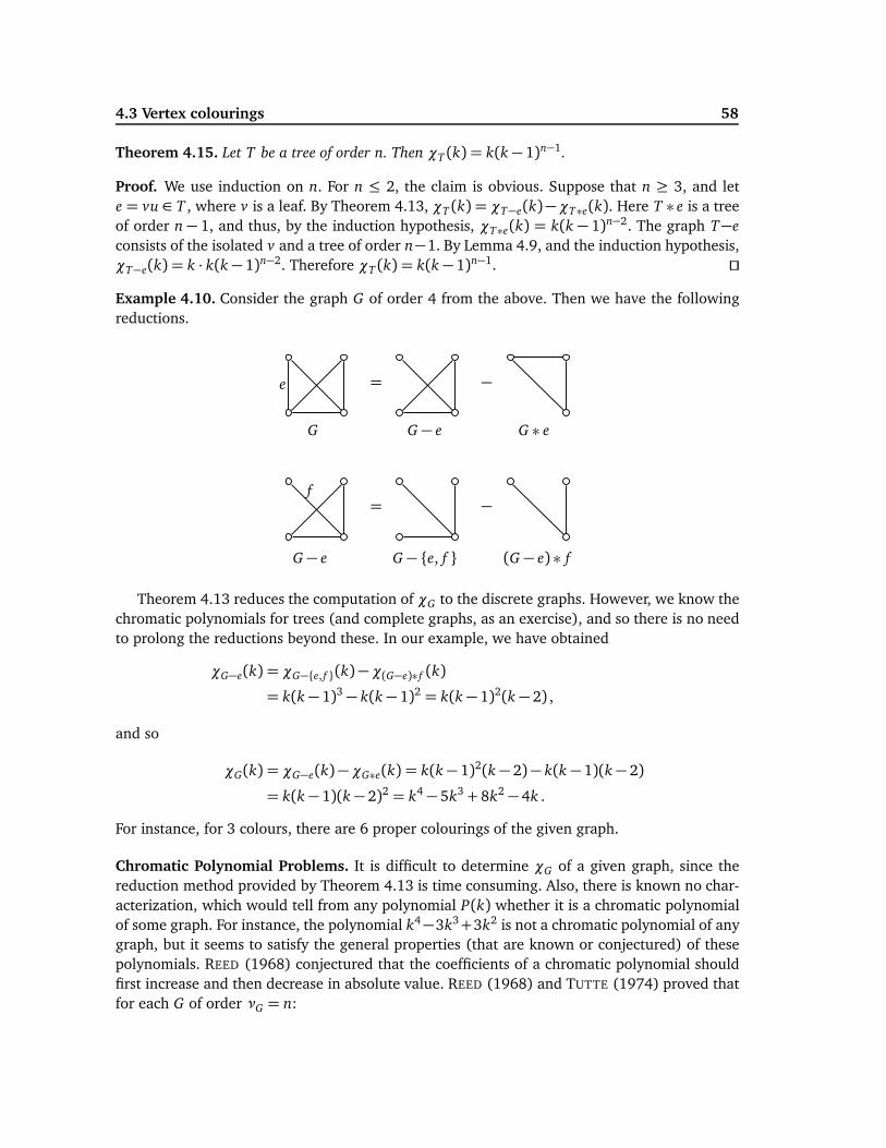
4.3 Vertex colourings 58
Theorem 4.15. Let T be a tree of order n. Then χT (k) = k(k − 1)n−1.
Proof. We use induction on n. For n ≤ 2, the claim is obvious. Suppose that n ≥ 3, and lete = vu ∈ T , where v is a leaf. By Theorem 4.13, χT (k) = χT−e(k)−χT∗e(k). Here T ∗ e is a treeof order n − 1, and thus, by the induction hypothesis, χT∗e(k) = k(k − 1)n−2. The graph T−e
consists of the isolated v and a tree of order n−1. By Lemma 4.9, and the induction hypothesis,χT−e(k) = k · k(k − 1)n−2. Therefore χT (k) = k(k − 1)n−1. ⊓⊔
Example 4.10. Consider the graph G of order 4 from the above. Then we have the followingreductions.
= −
G G − e G ∗ e
e
= −
G − e G − {e, f } (G − e) ∗ f
f
Theorem 4.13 reduces the computation of χG to the discrete graphs. However, we know thechromatic polynomials for trees (and complete graphs, as an exercise), and so there is no needto prolong the reductions beyond these. In our example, we have obtained
χG−e(k) = χG−{e, f }(k)−χ(G−e)∗ f (k)
= k(k − 1)3 − k(k − 1)2 = k(k − 1)2(k − 2) ,
and so
χG(k) = χG−e(k)−χG∗e(k) = k(k− 1)2(k − 2)− k(k − 1)(k− 2)
= k(k − 1)(k − 2)2 = k4 − 5k3 + 8k2 − 4k .
For instance, for 3 colours, there are 6 proper colourings of the given graph.
Chromatic Polynomial Problems. It is difficult to determine χG of a given graph, since thereduction method provided by Theorem 4.13 is time consuming. Also, there is known no char-acterization, which would tell from any polynomial P(k) whether it is a chromatic polynomialof some graph. For instance, the polynomial k4−3k3+3k2 is not a chromatic polynomial of anygraph, but it seems to satisfy the general properties (that are known or conjectured) of thesepolynomials. REED (1968) conjectured that the coefficients of a chromatic polynomial shouldfirst increase and then decrease in absolute value. REED (1968) and TUTTE (1974) proved thatfor each G of order νG = n:
4.3 Vertex colourings 59
• The degree of χG(k) equals n.• The coefficient of kn equals 1.• The coefficient of kn−1 equals −ǫG.• The constant term is 0.• The coefficients alternate in sign.• χG(m) ≤ m(m− 1)n − 1 for all positive integers m, when G is connected.• χG(x) 6= 0 for all real numbers 0< x < 1.
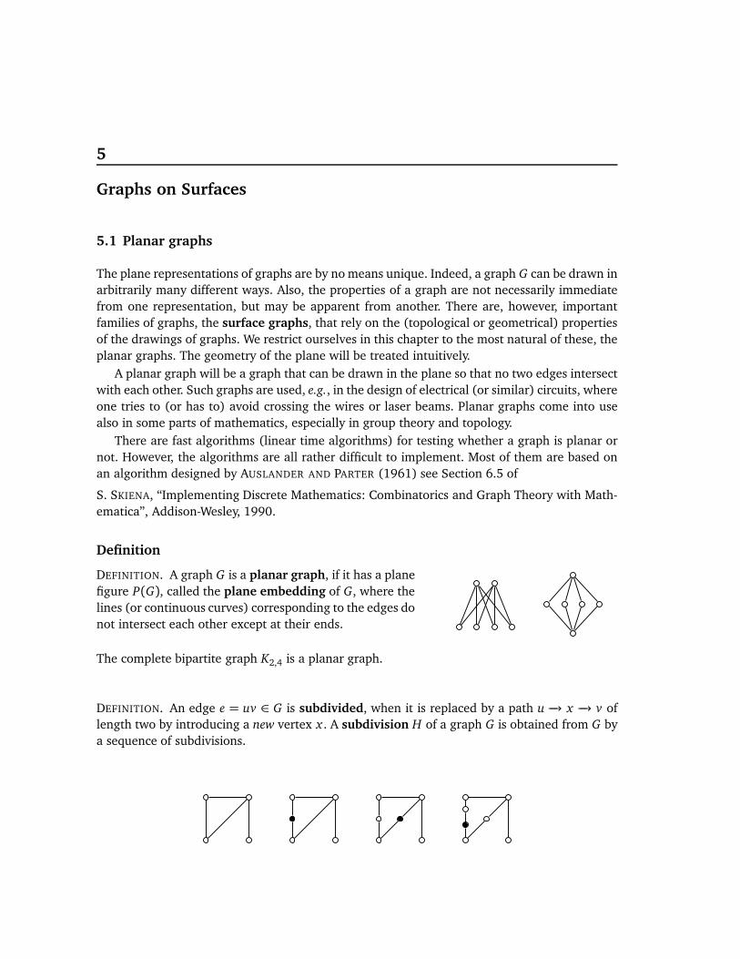
5
Graphs on Surfaces
5.1 Planar graphs
The plane representations of graphs are by no means unique. Indeed, a graph G can be drawn inarbitrarily many different ways. Also, the properties of a graph are not necessarily immediatefrom one representation, but may be apparent from another. There are, however, importantfamilies of graphs, the surface graphs, that rely on the (topological or geometrical) propertiesof the drawings of graphs. We restrict ourselves in this chapter to the most natural of these, theplanar graphs. The geometry of the plane will be treated intuitively.
A planar graph will be a graph that can be drawn in the plane so that no two edges intersectwith each other. Such graphs are used, e.g., in the design of electrical (or similar) circuits, whereone tries to (or has to) avoid crossing the wires or laser beams. Planar graphs come into usealso in some parts of mathematics, especially in group theory and topology.
There are fast algorithms (linear time algorithms) for testing whether a graph is planar ornot. However, the algorithms are all rather difficult to implement. Most of them are based onan algorithm designed by AUSLANDER AND PARTER (1961) see Section 6.5 of
S. SKIENA, “Implementing Discrete Mathematics: Combinatorics and Graph Theory with Math-ematica”, Addison-Wesley, 1990.
Definition
DEFINITION. A graph G is a planar graph, if it has a planefigure P(G), called the plane embedding of G, where thelines (or continuous curves) corresponding to the edges donot intersect each other except at their ends.
The complete bipartite graph K2,4 is a planar graph.
DEFINITION. An edge e = uv ∈ G is subdivided, when it is replaced by a path u −→ x −→ v oflength two by introducing a new vertex x . A subdivision H of a graph G is obtained from G bya sequence of subdivisions.
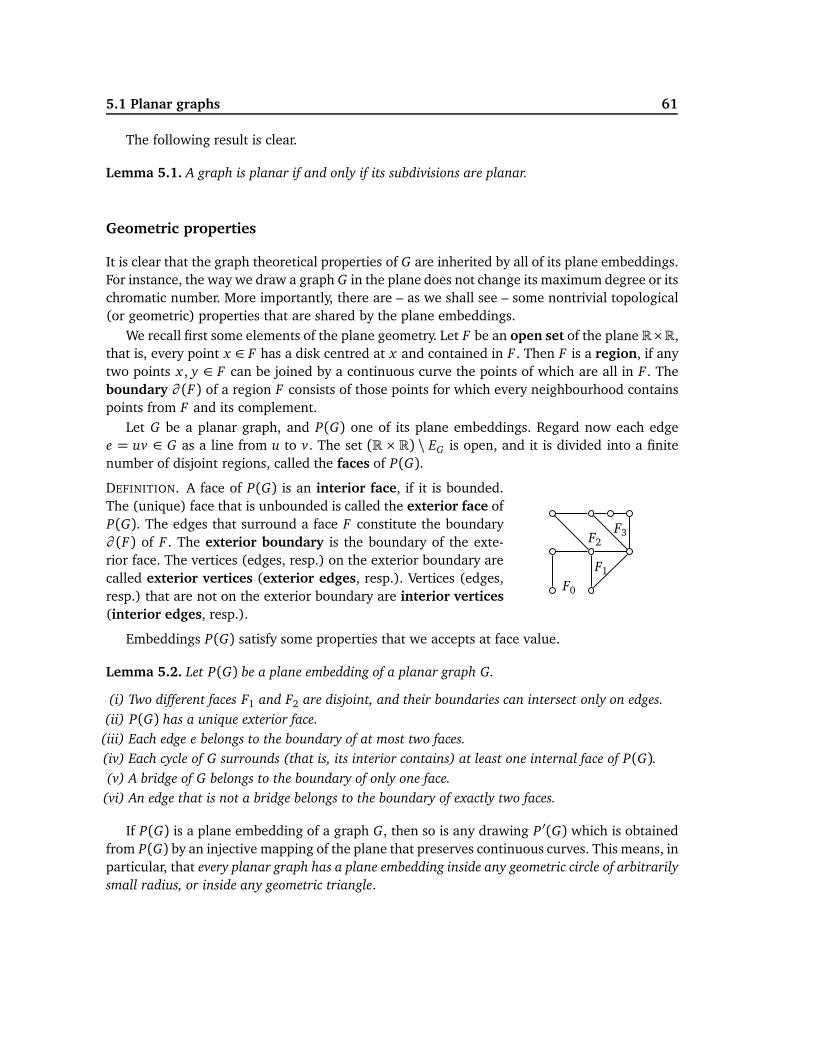
5.1 Planar graphs 61
The following result is clear.
Lemma 5.1. A graph is planar if and only if its subdivisions are planar.
Geometric properties
It is clear that the graph theoretical properties of G are inherited by all of its plane embeddings.For instance, the way we draw a graph G in the plane does not change its maximum degree or itschromatic number. More importantly, there are – as we shall see – some nontrivial topological(or geometric) properties that are shared by the plane embeddings.
We recall first some elements of the plane geometry. Let F be an open set of the plane R×R,that is, every point x ∈ F has a disk centred at x and contained in F . Then F is a region, if anytwo points x , y ∈ F can be joined by a continuous curve the points of which are all in F . Theboundary ∂ (F) of a region F consists of those points for which every neighbourhood containspoints from F and its complement.
Let G be a planar graph, and P(G) one of its plane embeddings. Regard now each edgee = uv ∈ G as a line from u to v. The set (R × R) \ EG is open, and it is divided into a finitenumber of disjoint regions, called the faces of P(G).
DEFINITION. A face of P(G) is an interior face, if it is bounded.The (unique) face that is unbounded is called the exterior face ofP(G). The edges that surround a face F constitute the boundary∂ (F) of F . The exterior boundary is the boundary of the exte-rior face. The vertices (edges, resp.) on the exterior boundary arecalled exterior vertices (exterior edges, resp.). Vertices (edges,resp.) that are not on the exterior boundary are interior vertices(interior edges, resp.).
F0
F1
F3F2
Embeddings P(G) satisfy some properties that we accepts at face value.
Lemma 5.2. Let P(G) be a plane embedding of a planar graph G.
(i) Two different faces F1 and F2 are disjoint, and their boundaries can intersect only on edges.
(ii) P(G) has a unique exterior face.
(iii) Each edge e belongs to the boundary of at most two faces.
(iv) Each cycle of G surrounds (that is, its interior contains) at least one internal face of P(G).
(v) A bridge of G belongs to the boundary of only one face.
(vi) An edge that is not a bridge belongs to the boundary of exactly two faces.
If P(G) is a plane embedding of a graph G, then so is any drawing P ′(G) which is obtainedfrom P(G) by an injective mapping of the plane that preserves continuous curves. This means, inparticular, that every planar graph has a plane embedding inside any geometric circle of arbitrarily
small radius, or inside any geometric triangle.
5.1 Planar graphs 62
Euler’s formula
Lemma 5.3. A plane embedding P(G) of a planar graph G has no interior faces if and only if G is
acyclic, that is, if and only if the connected components of G are trees.
Proof. This is clear from Lemma 5.2. ⊓⊔
The next general form of Euler’s formula was proved by LEGENDRE (1794).
Theorem 5.1 (Euler’s formula). Let G be a connected planar graph, and let P(G) be any of its
plane embeddings. Then
νG − ǫG +ϕ = 2 ,
where ϕ is the number of faces of P(G).
Proof. We shall prove the claim by induction on the number of faces ϕ of a plane embeddingP(G). First, notice that ϕ ≥ 1, since each P(G) has an exterior face.
If ϕ = 1, then, by Lemma 5.3, there are no cycles in G, and since G is connected, it is a tree.In this case, by Theorem 2.4, we have ǫG = νG − 1, and the claim holds.
Suppose then that the claim is true for all plane embeddings with less than ϕ faces forϕ ≥ 2.Let P(G) be a plane embedding of a connected planar graph such that P(G) has ϕ faces.
Let e ∈ G be an edge that is not a bridge. The subgraph G−e is planar with a plane embeddingP(G−e) = P(G)−e obtained by simply erasing the edge e. Now P(G−e) has ϕ−1 faces, since thetwo faces of P(G) that are separated by e are merged into one face of P(G−e). By the inductionhypothesis, νG−e − ǫG−e + (ϕ − 1) = 2, and hence νG − (ǫG − 1) + (ϕ − 1) = 2, and the claimfollows. ⊓⊔
In particular, we have the following invariant property of planar graphs.
Corollary 5.1. Let G be a planar graph. Then every plane embedding of G has the same number
of faces:
ϕG = ǫG − νG + 2
Maximal planar graphs
Lemma 5.4. If G is a planar graph of order νG ≥ 3, then ǫG ≤ 3νG − 6. Moreover, if G has no
triangles C3, then ǫG ≤ 2νG − 4.
Proof. If G is disconnected with connected components Gi, for i ∈ [1, k], and if the claim holdsfor these smaller (necessarily planar) graphs Gi , then it holds for G, since
ǫG =
νG∑
i=1
ǫGi≤ 3
νG∑
i=1
νGi− 6k = 3νG − 6k ≤ 3νG − 6 .
It is thus sufficient to prove the claim for connected planar graphs.
5.1 Planar graphs 63
Also, the case where ǫG ≤ 2 is clear. Suppose thus that ǫG ≥ 3.Each face F of an embedding P(G) contains at least three edges on its boundary ∂ (F). Hence
3ϕ ≤ 2ǫG, since each edge lies on at most two faces. The first claim follows from Euler’s formula.The second claim is proved similarly except that, in this case, each face F of P(G) contains
at least four edges on its boundary (when G is connected and ǫG ≥ 4). ⊓⊔
An upper bound for δ(G) for planar graphs was achieved by HEAWOOD.
Theorem 5.2 (HEAWOOD (1890)). If G is a planar graph, then δ(G) ≤ 5.
Proof. If νG ≤ 2, then there is nothing to prove. Suppose νG ≥ 3. By the handshaking lemmaand the previous lemma,
δ(G) · νG ≤∑
v∈G
dG(v) = 2ǫG ≤ 6νG − 12 .
It follows that δ(G) ≤ 5. ⊓⊔
Theorem 5.3. K5 and K3,3 are not planar graphs.
Proof. By Lemma 5.4, a planar graph of order 5 has at most 9 edges, but K5 has 5 vertices and10 edges. By the second claim of Lemma 5.4, a triangle-free planar graph of order 6 has at most8 edges, but K3,3 has 6 vertices and 9 edges. ⊓⊔
DEFINITION. A planar graph G is maximal, if G + e is nonplanar for every e /∈ G.
Example 5.1. Clearly, if we remove one edge from K5, the result is a maximal planar graph.However, if an edge is removed from K3,3, the result is not maximal!
Lemma 5.5. Let F be a face of a plane embedding P(G) that has at least four edges on its boundary.
Then there are two nonadjacent vertices on the boundary of F.
Proof. Assume that the set of the boundary vertices of F induces a complete subgraph K . Theedges of K are either on the boundary or they are not inside F (since F is a face.) Add a newvertex x inside F , and connect the vertices of K to x . The result is a plane embedding of a graphH with VH = VG ∪ {x} (that has G as its induced subgraph). The induced subgraph H[K ∪ {x}]
is complete, and since H is planar, we have |K |< 4 as required. ⊓⊔
By the previous lemma, if a face has a boundary of at least four edges, then an edge canbe added to the graph (inside the face), and the graph remains to be planar. Hence we haveproved
Corollary 5.2. If G is a maximal planar graph with νG ≥ 3, then G is triangulated, that is, every
face of a plane embedding P(G) has a boundary of exactly three edges.
Theorem 5.4. For a maximal planar graph G of order νG ≥ 3, ǫG = 3νG − 6 .
Proof. Each face F of an embedding P(G) is a triangle having three edges on its boundary.Hence 3ϕ = 2ǫG, since there are now no bridges. The claim follows from Euler’s formula. ⊓⊔
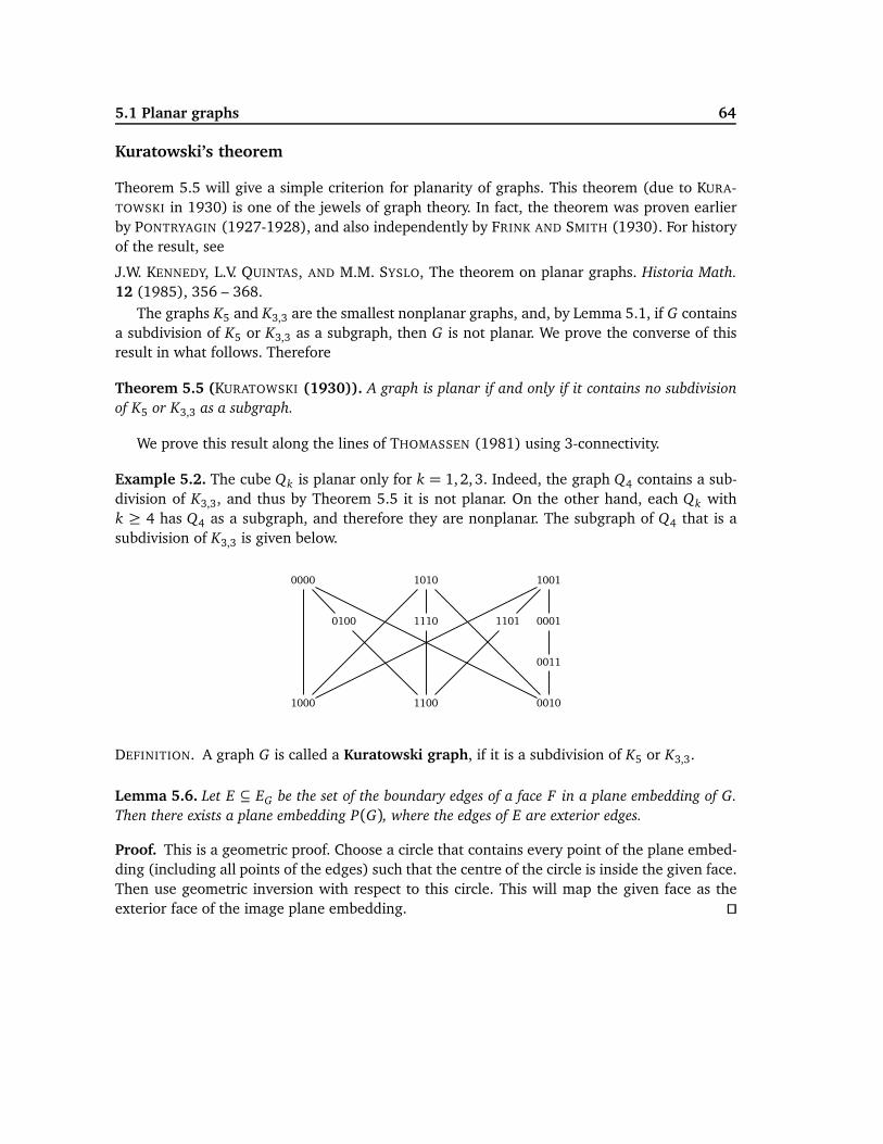
5.1 Planar graphs 64
Kuratowski’s theorem
Theorem 5.5 will give a simple criterion for planarity of graphs. This theorem (due to KURA-TOWSKI in 1930) is one of the jewels of graph theory. In fact, the theorem was proven earlierby PONTRYAGIN (1927-1928), and also independently by FRINK AND SMITH (1930). For historyof the result, see
J.W. KENNEDY, L.V. QUINTAS, AND M.M. SYSLO, The theorem on planar graphs. Historia Math.
12 (1985), 356 – 368.The graphs K5 and K3,3 are the smallest nonplanar graphs, and, by Lemma 5.1, if G contains
a subdivision of K5 or K3,3 as a subgraph, then G is not planar. We prove the converse of thisresult in what follows. Therefore
Theorem 5.5 (KURATOWSKI (1930)). A graph is planar if and only if it contains no subdivision
of K5 or K3,3 as a subgraph.
We prove this result along the lines of THOMASSEN (1981) using 3-connectivity.
Example 5.2. The cube Qk is planar only for k = 1,2,3. Indeed, the graph Q4 contains a sub-division of K3,3, and thus by Theorem 5.5 it is not planar. On the other hand, each Qk withk ≥ 4 has Q4 as a subgraph, and therefore they are nonplanar. The subgraph of Q4 that is asubdivision of K3,3 is given below.
1000 1100 0010
0000 1010 1001
0100 1110 1101 0001
0011
DEFINITION. A graph G is called a Kuratowski graph, if it is a subdivision of K5 or K3,3.
Lemma 5.6. Let E ⊆ EG be the set of the boundary edges of a face F in a plane embedding of G.
Then there exists a plane embedding P(G), where the edges of E are exterior edges.
Proof. This is a geometric proof. Choose a circle that contains every point of the plane embed-ding (including all points of the edges) such that the centre of the circle is inside the given face.Then use geometric inversion with respect to this circle. This will map the given face as theexterior face of the image plane embedding. ⊓⊔
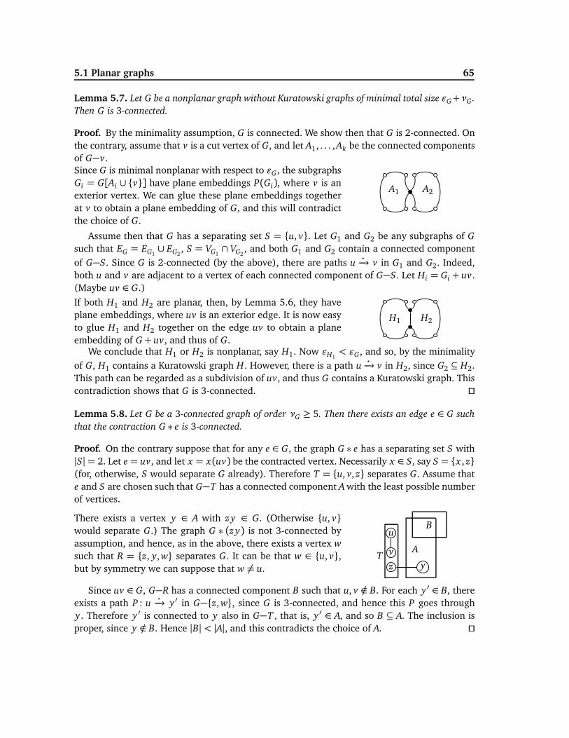
5.1 Planar graphs 65
Lemma 5.7. Let G be a nonplanar graph without Kuratowski graphs of minimal total size ǫG+νG .
Then G is 3-connected.
Proof. By the minimality assumption, G is connected. We show then that G is 2-connected. Onthe contrary, assume that v is a cut vertex of G, and let A1, . . . ,Ak be the connected componentsof G−v.Since G is minimal nonplanar with respect to ǫG, the subgraphsGi = G[Ai ∪ {v}] have plane embeddings P(Gi), where v is anexterior vertex. We can glue these plane embeddings togetherat v to obtain a plane embedding of G, and this will contradictthe choice of G.
A1 A2
Assume then that G has a separating set S = {u, v}. Let G1 and G2 be any subgraphs of G
such that EG = EG1∪ EG2
, S = VG1∩ VG2
, and both G1 and G2 contain a connected componentof G−S. Since G is 2-connected (by the above), there are paths u
⋆−→ v in G1 and G2. Indeed,
both u and v are adjacent to a vertex of each connected component of G−S. Let Hi = Gi + uv.(Maybe uv ∈ G.)
If both H1 and H2 are planar, then, by Lemma 5.6, they haveplane embeddings, where uv is an exterior edge. It is now easyto glue H1 and H2 together on the edge uv to obtain a planeembedding of G + uv, and thus of G.
H1 H2
We conclude that H1 or H2 is nonplanar, say H1. Now ǫH1< ǫG, and so, by the minimality
of G, H1 contains a Kuratowski graph H. However, there is a path u⋆−→ v in H2, since G2 ⊆ H2.
This path can be regarded as a subdivision of uv, and thus G contains a Kuratowski graph. Thiscontradiction shows that G is 3-connected. ⊓⊔
Lemma 5.8. Let G be a 3-connected graph of order νG ≥ 5. Then there exists an edge e ∈ G such
that the contraction G ∗ e is 3-connected.
Proof. On the contrary suppose that for any e ∈ G, the graph G ∗ e has a separating set S with|S| = 2. Let e = uv, and let x = x(uv) be the contracted vertex. Necessarily x ∈ S, say S = {x , z}(for, otherwise, S would separate G already). Therefore T = {u, v, z} separates G. Assume thate and S are chosen such that G−T has a connected component A with the least possible numberof vertices.
There exists a vertex y ∈ A with z y ∈ G. (Otherwise {u, v}
would separate G.) The graph G ∗ (z y) is not 3-connected byassumption, and hence, as in the above, there exists a vertex w
such that R = {z, y, w} separates G. It can be that w ∈ {u, v},but by symmetry we can suppose that w 6= u.
u
v
z y
B
TA
Since uv ∈ G, G−R has a connected component B such that u, v /∈ B. For each y ′ ∈ B, thereexists a path P : u
⋆−→ y ′ in G−{z, w}, since G is 3-connected, and hence this P goes through
y. Therefore y ′ is connected to y also in G−T , that is, y ′ ∈ A, and so B ⊆ A. The inclusion isproper, since y /∈ B. Hence |B| < |A|, and this contradicts the choice of A. ⊓⊔
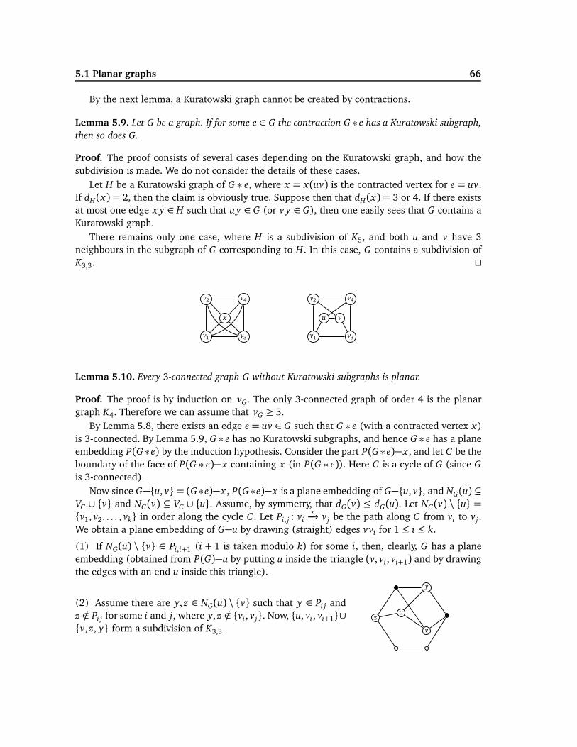
5.1 Planar graphs 66
By the next lemma, a Kuratowski graph cannot be created by contractions.
Lemma 5.9. Let G be a graph. If for some e ∈ G the contraction G ∗ e has a Kuratowski subgraph,
then so does G.
Proof. The proof consists of several cases depending on the Kuratowski graph, and how thesubdivision is made. We do not consider the details of these cases.
Let H be a Kuratowski graph of G ∗ e, where x = x(uv) is the contracted vertex for e = uv.If dH(x) = 2, then the claim is obviously true. Suppose then that dH(x) = 3 or 4. If there existsat most one edge x y ∈ H such that uy ∈ G (or v y ∈ G), then one easily sees that G contains aKuratowski graph.
There remains only one case, where H is a subdivision of K5, and both u and v have 3neighbours in the subgraph of G corresponding to H. In this case, G contains a subdivision ofK3,3. ⊓⊔
v1
v2
x
v3
v4
v1
v2
u v
v3
v4
Lemma 5.10. Every 3-connected graph G without Kuratowski subgraphs is planar.
Proof. The proof is by induction on νG. The only 3-connected graph of order 4 is the planargraph K4. Therefore we can assume that νG ≥ 5.
By Lemma 5.8, there exists an edge e = uv ∈ G such that G ∗ e (with a contracted vertex x)is 3-connected. By Lemma 5.9, G ∗ e has no Kuratowski subgraphs, and hence G ∗ e has a planeembedding P(G ∗ e) by the induction hypothesis. Consider the part P(G ∗ e)−x , and let C be theboundary of the face of P(G ∗ e)−x containing x (in P(G ∗ e)). Here C is a cycle of G (since G
is 3-connected).Now since G−{u, v} = (G∗e)−x , P(G∗e)−x is a plane embedding of G−{u, v}, and NG(u) ⊆
VC ∪ {v} and NG(v) ⊆ VC ∪ {u}. Assume, by symmetry, that dG(v) ≤ dG(u). Let NG(v) \ {u} =
{v1, v2, . . . , vk} in order along the cycle C . Let Pi, j : vi⋆−→ v j be the path along C from vi to v j .
We obtain a plane embedding of G−u by drawing (straight) edges vvi for 1≤ i ≤ k.
(1) If NG(u) \ {v} ∈ Pi,i+1 (i + 1 is taken modulo k) for some i, then, clearly, G has a planeembedding (obtained from P(G)−u by putting u inside the triangle (v, vi, vi+1) and by drawingthe edges with an end u inside this triangle).
(2) Assume there are y, z ∈ NG(u) \ {v} such that y ∈ Pi j andz /∈ Pi j for some i and j, where y, z /∈ {vi, v j}. Now, {u, vi , vi+1}∪
{v, z, y} form a subdivision of K3,3. v
u
y
z

5.2 Colouring planar graphs 67
By (1) and (2), we can assume that NG(u)\{v} ⊆ NG(v). There-fore, NG(u)\{v} = NG(v)\{u} by the assumption dG(v)≤ dG(u).Also, by (1), dG(v) = dG(u) > 3. But now u, v, v1, v2, v3 give asubdivision of K5. ⊓⊔
v
u
Proof of Theorem 5.5. By Theorem 5.3 and Lemma 5.1, we need to show that each nonplanargraph G contains a Kuratowski subgraph. On the contrary, suppose that G is a nonplanar graphthat has a minimal size ǫG such that G does not contain a Kuratowski subgraph. Then, byLemma 5.7, G is 3-connected, and by Lemma 5.10, it is planar. This contradiction proves theclaim. ⊓⊔
Example 5.3. Any graph G can be drawn in the plane so that three of its edges never intersectat the same point. The crossing number ×(G) is the minimum number of intersections of itsedges in such plane drawings of G. Therefore G is planar if and only if ×(G) = 0, and, forinstance, ×(K5) = 1.
We show that ×(K6) = 3. For this we need to show that ×(K6) ≥ 3. For the equality, one isinvited to design a drawing with exactly 3 crossings.
Let X (K6) be a drawing of K6 using c crossings so that two edges cross at most once. Adda new vertex at each crossing. This results in a planar graph G on c + 6 vertices and 2c + 15edges. Now c ≥ 3, since ǫG = 2c + 15≤ 3(c + 6)− 6= 3νG − 6.
5.2 Colouring planar graphs
The most famous problem in the history of graph theory is that of the chromatic number ofplanar graphs. The problem was known as the 4-Colour Conjecture for more than 120 years,until it was solved by APPEL AND HAKEN in 1976: if G is a planar graph, then χ(G) ≤ 4. The4-Colour Conjecture has had a deep influence on the theory of graphs during the last 150 years.The solution of the 4-Colour Theorem is difficult, and it requires the assistance of a computer.
The 5-colour theorem
We prove HEAWOOD’s result (1890) that each planar graph is properly 5-colourable.
Lemma 5.11. If G is a planar graph, then χ(G) ≤ 6.
Proof. The proof is by induction on νG. Clearly, the claim holds for νG ≤ 6. By Theorem 5.2, aplanar graph G has a vertex v with dG(v)≤ 5. By the induction hypothesis, χ(G−v)≤ 6. SincedG(v)≤ 5, there is a colour i available for v in the 6-colouring of G−v, and so χ(G) ≤ 6. ⊓⊔
The proof of the following theorem is partly geometric in nature.
Theorem 5.6 (HEAWOOD (1890)). If G is a planar graph, then χ(G) ≤ 5.
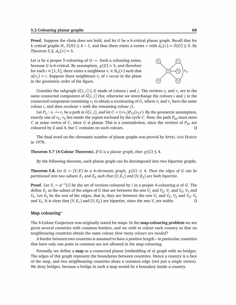
5.2 Colouring planar graphs 68
Proof. Suppose the claim does not hold, and let G be a 6-critical planar graph. Recall that fork-critical graphs H, δ(H) ≥ k − 1, and thus there exists a vertex v with dG(v) = δ(G) ≥ 5. ByTheorem 5.2, dG(v) = 5.
Let α be a proper 5-colouring of G−v. Such a colouring exists,because G is 6-critical. By assumption, χ(G) > 5, and thereforefor each i ∈ [1,5], there exists a neighbour vi ∈ NG(v) such thatα(vi) = i. Suppose these neighbours vi of v occur in the planein the geometric order of the figure.
v
v4
v5
v3
v2
v1
P13
Consider the subgraph G[i, j] ⊆ G made of colours i and j. The vertices vi and v j are in thesame connected component of G[i, j] (for, otherwise we interchange the colours i and j in theconnected component containing v j to obtain a recolouring of G, where vi and v j have the samecolour i, and then recolour v with the remaining colour j).
Let Pi j : vi⋆−→ v j be a path in G[i, j], and let C = (vv1)P13(v3v). By the geometric assumption,
exactly one of v2, v4 lies inside the region enclosed by the cycle C . Now, the path P24 must meetC at some vertex of C , since G is planar. This is a contradiction, since the vertices of P24 arecoloured by 2 and 4, but C contains no such colours. ⊓⊔
The final word on the chromatic number of planar graphs was proved by APPEL AND HAKEN
in 1976.
Theorem 5.7 (4-Colour Theorem). If G is a planar graph, then χ(G) ≤ 4.
By the following theorem, each planar graph can be decomposed into two bipartite graphs.
Theorem 5.8. Let G = (V, E) be a 4-chromatic graph, χ(G) ≤ 4. Then the edges of G can be
partitioned into two subsets E1 and E2 such that (V, E1) and (V, E2) are both bipartite.
Proof. Let Vi = α−1(i) be the set of vertices coloured by i in a proper 4-colouring α of G. The
define E1 as the subset of the edges of G that are between the sets V1 and V2; V1 and V4; V3 andV4. Let E2 be the rest of the edges, that is, they are between the sets V1 and V3; V2 and V3; V2
and V4. It is clear that (V, E1) and (V, E2) are bipartite, since the sets Vi are stable. ⊓⊔
Map colouring∗
The 4-Colour Conjecture was originally stated for maps. In the map-colouring problem we aregiven several countries with common borders, and we wish to colour each country so that noneighbouring countries obtain the same colour. How many colours are needed?
A border between two countries is assumed to have a positive length – in particular, countriesthat have only one point in common are not allowed in the map colouring.
Formally, we define a map as a connected planar (embedding of a) graph with no bridges.The edges of this graph represent the boundaries between countries. Hence a country is a faceof the map, and two neighbouring countries share a common edge (not just a single vertex).We deny bridges, because a bridge in such a map would be a boundary inside a country.
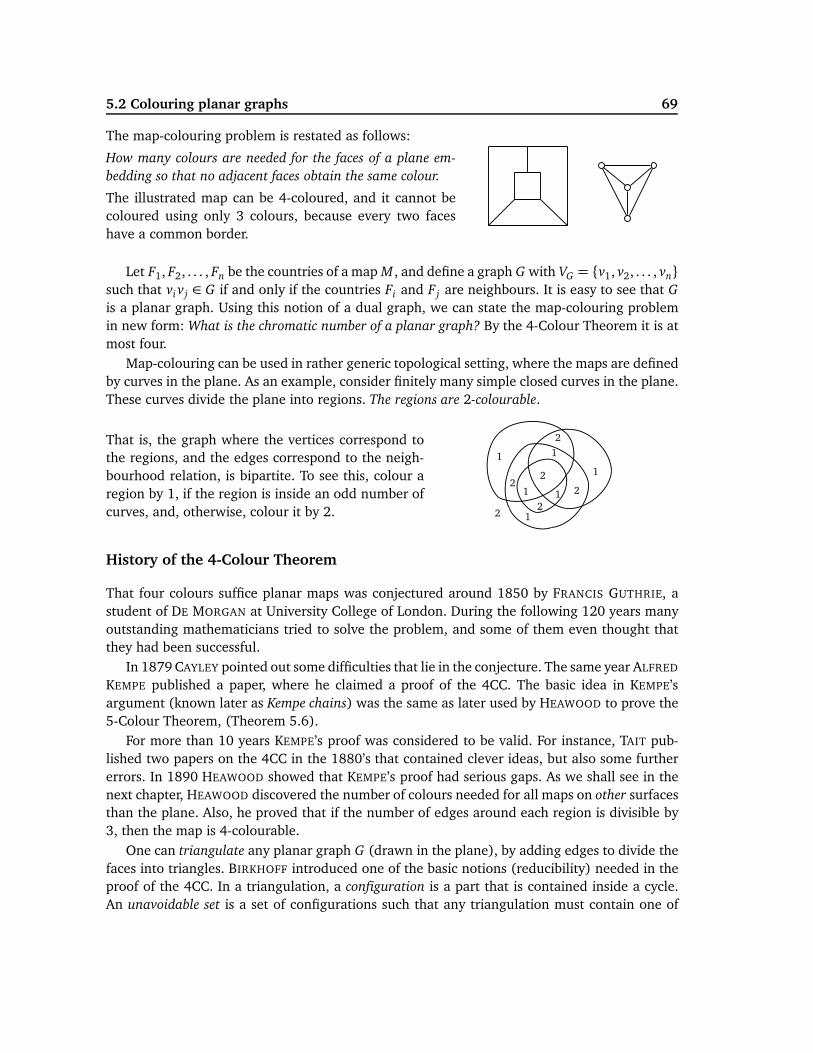
5.2 Colouring planar graphs 69
The map-colouring problem is restated as follows:
How many colours are needed for the faces of a plane em-
bedding so that no adjacent faces obtain the same colour.
The illustrated map can be 4-coloured, and it cannot becoloured using only 3 colours, because every two faceshave a common border.
Let F1, F2, . . . , Fn be the countries of a map M , and define a graph G with VG = {v1, v2, . . . , vn}
such that vi v j ∈ G if and only if the countries Fi and F j are neighbours. It is easy to see that G
is a planar graph. Using this notion of a dual graph, we can state the map-colouring problemin new form: What is the chromatic number of a planar graph? By the 4-Colour Theorem it is atmost four.
Map-colouring can be used in rather generic topological setting, where the maps are definedby curves in the plane. As an example, consider finitely many simple closed curves in the plane.These curves divide the plane into regions. The regions are 2-colourable.
That is, the graph where the vertices correspond tothe regions, and the edges correspond to the neigh-bourhood relation, is bipartite. To see this, colour aregion by 1, if the region is inside an odd number ofcurves, and, otherwise, colour it by 2. 2
1
2
12
1
2
1 2
1
1
2
History of the 4-Colour Theorem
That four colours suffice planar maps was conjectured around 1850 by FRANCIS GUTHRIE, astudent of DE MORGAN at University College of London. During the following 120 years manyoutstanding mathematicians tried to solve the problem, and some of them even thought thatthey had been successful.
In 1879 CAYLEY pointed out some difficulties that lie in the conjecture. The same year ALFRED
KEMPE published a paper, where he claimed a proof of the 4CC. The basic idea in KEMPE’sargument (known later as Kempe chains) was the same as later used by HEAWOOD to prove the5-Colour Theorem, (Theorem 5.6).
For more than 10 years KEMPE’s proof was considered to be valid. For instance, TAIT pub-lished two papers on the 4CC in the 1880’s that contained clever ideas, but also some furthererrors. In 1890 HEAWOOD showed that KEMPE’s proof had serious gaps. As we shall see in thenext chapter, HEAWOOD discovered the number of colours needed for all maps on other surfacesthan the plane. Also, he proved that if the number of edges around each region is divisible by3, then the map is 4-colourable.
One can triangulate any planar graph G (drawn in the plane), by adding edges to divide thefaces into triangles. BIRKHOFF introduced one of the basic notions (reducibility) needed in theproof of the 4CC. In a triangulation, a configuration is a part that is contained inside a cycle.An unavoidable set is a set of configurations such that any triangulation must contain one of
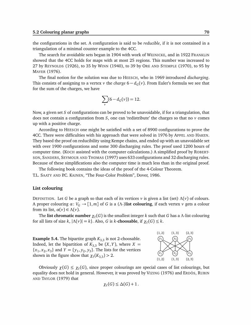
5.2 Colouring planar graphs 70
the configurations in the set. A configuration is said to be reducible, if it is not contained in atriangulation of a minimal counter example to the 4CC.
The search for avoidable sets began in 1904 with work of WEINICKE, and in 1922 FRANKLIN
showed that the 4CC holds for maps with at most 25 regions. This number was increased to27 by REYNOLDS (1926), to 35 by WINN (1940), to 39 by ORE AND STEMPLE (1970), to 95 byMAYER (1976).
The final notion for the solution was due to HEESCH, who in 1969 introduced discharging.This consists of assigning to a vertex v the charge 6− dG(v). From Euler’s formula we see thatfor the sum of the charges, we have
∑
v
(6− dG(v)) = 12.
Now, a given set S of configurations can be proved to be unavoidable, if for a triangulation, thatdoes not contain a configuration from S, one can ‘redistribute’ the charges so that no v comesup with a positive charge.
According to HEESCH one might be satisfied with a set of 8900 configurations to prove the4CC. There were difficulties with his approach that were solved in 1976 by APPEL AND HAKEN.They based the proof on reducibility using Kempe chains, and ended up with an unavoidable setwith over 1900 configurations and some 300 discharging rules. The proof used 1200 hours ofcomputer time. (KOCH assisted with the computer calculations.) A simplified proof by ROBERT-SON, SANDERS, SEYMOUR AND THOMAS (1997) uses 633 configurations and 32 discharging rules.Because of these simplifications also the computer time is much less than in the original proof.
The following book contains the ideas of the proof of the 4-Colour Theorem.T.L. SAATY AND P.C. KAINEN, “The Four-Color Problem”, Dover, 1986.
List colouring
DEFINITION. Let G be a graph so that each of its vertices v is given a list (set) Λ(v) of colours.A proper colouring α: VG → [1, m] of G is a (Λ-)list colouring, if each vertex v gets a colourfrom its list, α(v) ∈ Λ(v).
The list chromatic number χℓ(G) is the smallest integer k such that G has a Λ-list colouringfor all lists of size k, |Λ(v)| = k}. Also, G is k-choosable, if χℓ(G) ≤ k.
Example 5.4. The bipartite graph K3,3 is not 2-choosable.Indeed, let the bipartition of K3,3 be (X , Y ), where X =
{x1, x2, x3} and Y = {y1, y2, y3}. The lists for the verticesshown in the figure show that χℓ(K3,3) > 2.
x1
{1, 2}
y1
{1, 2}
x2
{1, 3}
y2
{1, 3}
x3
{2, 3}
y3
{2, 3}
Obviously χ(G) ≤ χℓ(G), since proper colourings are special cases of list colourings, butequality does not hold in general. However, it was proved by VIZING (1976) and ERDÖS, RUBIN
AND TAYLOR (1979) thatχℓ(G) ≤∆(G) + 1 .
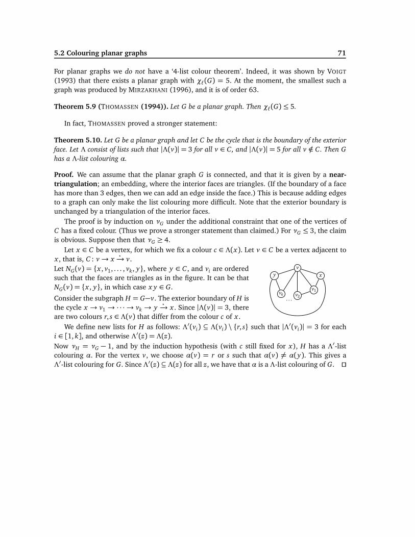
5.2 Colouring planar graphs 71
For planar graphs we do not have a ‘4-list colour theorem’. Indeed, it was shown by VOIGT
(1993) that there exists a planar graph with χℓ(G) = 5. At the moment, the smallest such agraph was produced by MIRZAKHANI (1996), and it is of order 63.
Theorem 5.9 (THOMASSEN (1994)). Let G be a planar graph. Then χℓ(G) ≤ 5.
In fact, THOMASSEN proved a stronger statement:
Theorem 5.10. Let G be a planar graph and let C be the cycle that is the boundary of the exterior
face. Let Λ consist of lists such that |Λ(v)| = 3 for all v ∈ C, and |Λ(v)| = 5 for all v /∈ C. Then G
has a Λ-list colouring α.
Proof. We can assume that the planar graph G is connected, and that it is given by a near-triangulation; an embedding, where the interior faces are triangles. (If the boundary of a facehas more than 3 edges, then we can add an edge inside the face.) This is because adding edgesto a graph can only make the list colouring more difficult. Note that the exterior boundary isunchanged by a triangulation of the interior faces.
The proof is by induction on νG under the additional constraint that one of the vertices ofC has a fixed colour. (Thus we prove a stronger statement than claimed.) For νG ≤ 3, the claimis obvious. Suppose then that νG ≥ 4.
Let x ∈ C be a vertex, for which we fix a colour c ∈ Λ(x). Let v ∈ C be a vertex adjacent tox , that is, C : v→ x
⋆−→ v.
Let NG(v) = {x , v1, . . . , vk, y}, where y ∈ C , and vi are orderedsuch that the faces are triangles as in the figure. It can be thatNG(v) = {x , y}, in which case x y ∈ G.
Consider the subgraph H = G−v. The exterior boundary of H isthe cycle x → v1 → · · · → vk → y
⋆−→ x . Since |Λ(v)| = 3, there
are two colours r, s ∈ Λ(v) that differ from the colour c of x .
v
xy
v1v2
vk
. . .
We define new lists for H as follows: Λ′(vi) ⊆ Λ(vi) \ {r, s} such that |Λ′(vi)| = 3 for eachi ∈ [1, k], and otherwise Λ′(z) = Λ(z).Now νH = νG − 1, and by the induction hypothesis (with c still fixed for x), H has a Λ′-listcolouring α. For the vertex v, we choose α(v) = r or s such that α(v) 6= α(y). This gives aΛ′-list colouring for G. Since Λ′(z) ⊆ Λ(z) for all z, we have that α is a Λ-list colouring of G. ⊓⊔
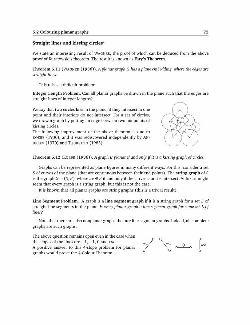
5.2 Colouring planar graphs 72
Straight lines and kissing circles∗
We state an interesting result of WAGNER, the proof of which can be deduced from the aboveproof of Kuratowski’s theorem. The result is known as Fáry’s Theorem.
Theorem 5.11 (WAGNER (1936)). A planar graph G has a plane embedding, where the edges are
straight lines.
This raises a difficult problem:
Integer Length Problem. Can all planar graphs be drawn in the plane such that the edges arestraight lines of integer lengths?
We say that two circles kiss in the plane, if they intersect in onepoint and their interiors do not intersect. For a set of circles,we draw a graph by putting an edge between two midpoints ofkissing circles.The following improvement of the above theorem is due toKOEBE (1936), and it was rediscovered independently by AN-DREEV (1970) and THURSTON (1985).
· ·
· ·
··
·
·
Theorem 5.12 (KOEBE (1936)). A graph is planar if and only if it is a kissing graph of circles.
Graphs can be represented as plane figures in many different ways. For this, consider a setS of curves of the plane (that are continuous between their end points). The string graph of S
is the graph G = (S, E), where uv ∈ E if and only if the curves u and v intersect. At first it mightseem that every graph is a string graph, but this is not the case.
It is known that all planar graphs are string graphs (this is a trivial result).
Line Segment Problem. A graph is a line segment graph if it is a string graph for a set L ofstraight line segments in the plane. Is every planar graph a line segment graph for some set L of
lines?
Note that there are also nonplanar graphs that are line segment graphs. Indeed, all completegraphs are such graphs.
The above question remains open even in the case whenthe slopes of the lines are +1, −1, 0 and∞.A positive answer to this 4-slope problem for planargraphs would prove the 4-Colour Theorem.
+1 −1 0 ∞
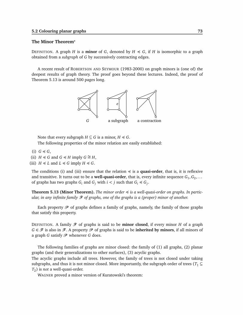
5.2 Colouring planar graphs 73
The Minor Theorem∗
DEFINITION. A graph H is a minor of G, denoted by H ´ G, if H is isomorphic to a graphobtained from a subgraph of G by successively contracting edges.
A recent result of ROBERTSON AND SEYMOUR (1983-2000) on graph minors is (one of) thedeepest results of graph theory. The proof goes beyond these lectures. Indeed, the proof ofTheorem 5.13 is around 500 pages long.
G a subgraph a contraction
e
Note that every subgraph H ⊆ G is a minor, H ´ G.The following properties of the minor relation are easily established:
(i) G ´ G,(ii) H ´ G and G ´ H imply G ∼= H,(iii) H ´ L and L ´ G imply H ´ G.
The conditions (i) and (iii) ensure that the relation ´ is a quasi-order, that is, it is reflexiveand transitive. It turns out to be a well-quasi-order, that is, every infinite sequence G1, G2, . . .of graphs has two graphs Gi and G j with i < j such that Gi ´ G j .
Theorem 5.13 (Minor Theorem). The minor order ´ is a well-quasi-order on graphs. In partic-
ular, in any infinite family F of graphs, one of the graphs is a (proper) minor of another.
Each property P of graphs defines a family of graphs, namely, the family of those graphsthat satisfy this property.
DEFINITION. A family F of graphs is said to be minor closed, if every minor H of a graphG ∈ F is also in F . A property P of graphs is said to be inherited by minors, if all minors ofa graph G satisfy P whenever G does.
The following families of graphs are minor closed: the family of (1) all graphs, (2) planargraphs (and their generalizations to other surfaces), (3) acyclic graphs.The acyclic graphs include all trees. However, the family of trees is not closed under takingsubgraphs, and thus it is not minor closed. More importantly, the subgraph order of trees (T1 ⊆
T2) is not a well-quasi-order.WAGNER proved a minor version of Kuratowski’s theorem:
5.3 Genus of a graph 74
Theorem 5.14 (WAGNER (1937)). A graph G is nonplanar if and only if K5 ´ G or K3,3 ´ G.
Proof. Exercise. ⊓⊔
ROBERTSON AND SEYMOUR (1998) proved the Wagner’s conjecture:
Theorem 5.15 (Minor Theorem 2). Let P be a property of graphs inherited by minors. Then
there exists a finite set F of graphs such that G satisfies P if and only if G does not have a minor
from F .
One of the impressive application of Theorem 5.15 concerns embeddings of graphs on sur-faces, see the next chapters. By Theorem 5.15, one can test (with a fast algorithm) whether agraph can be embedded onto a surface.
Every graph can be drawn in the 3-dimensional space without crossing edges. An old problemasks if there exists an algorithm that would determine whether a graph can be drawn so thatits cycles do not form (nontrivial) knots. This problem is solved by the above results, since theproperty ‘knotless’ is inherited by minors: there exists a fast algorithm to do the job. However,this algorithm is not known!
Hadwiger’s Problem. HADWIGER conjectured in 1943 that for every graph G,
Kχ(G) ´ G ,
that is, if χ(G) ≥ r, then G has a complete graph Kr as its minor. The conjecture is trivial forr = 2, and it is known to hold for all r ≤ 6. The cases for r = 5 and 6 follow from the 4-ColourTheorem.
5.3 Genus of a graph
A graph is planar, if it can be drawn in the plane without crossing edges. A plane is an importantspecial case of a surface. In this section we study shortly drawing graphs in other surfaces.
There are quite many interesting surfaces many of which are rather difficult to draw. Weshall study the ‘easy surfaces’ – those that are compact and orientable. These are surfaces thathave both an inside and an outside, and can be entirely characterized by the number of holes inthem. This number is the genus of the surface. There are also non-orientable compact surfacessuch as the Klein bottle and the projective plane.
Background on surfaces
We shall first have a quick look at the general surfaces and their classification without goinginto the details. Consider the space R3, which has its (usual) distance function d(x , y) ∈ R ofits points.
Two figures (i.e., sets of points) A and B are topologically equivalent (or homeomorphic)if there exists a bijection f : A → B such that f and its inverse f −1 : B → A are continuous.
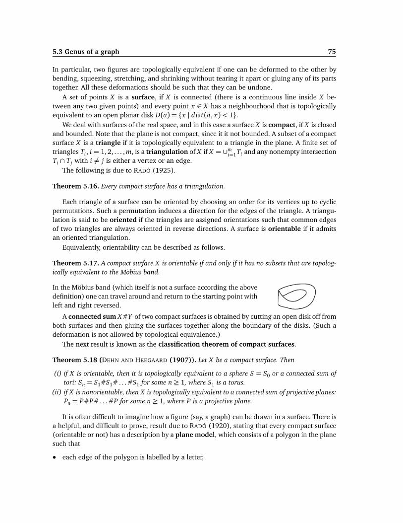
5.3 Genus of a graph 75
In particular, two figures are topologically equivalent if one can be deformed to the other bybending, squeezing, stretching, and shrinking without tearing it apart or gluing any of its partstogether. All these deformations should be such that they can be undone.
A set of points X is a surface, if X is connected (there is a continuous line inside X be-tween any two given points) and every point x ∈ X has a neighbourhood that is topologicallyequivalent to an open planar disk D(a) = {x | dist(a, x) < 1}.
We deal with surfaces of the real space, and in this case a surface X is compact, if X is closedand bounded. Note that the plane is not compact, since it it not bounded. A subset of a compactsurface X is a triangle if it is topologically equivalent to a triangle in the plane. A finite set oftriangles Ti , i = 1,2, . . . , m, is a triangulation of X if X = ∪m
i=1Ti and any nonempty intersectionTi ∩ T j with i 6= j is either a vertex or an edge.
The following is due to RADÓ (1925).
Theorem 5.16. Every compact surface has a triangulation.
Each triangle of a surface can be oriented by choosing an order for its vertices up to cyclicpermutations. Such a permutation induces a direction for the edges of the triangle. A triangu-lation is said to be oriented if the triangles are assigned orientations such that common edgesof two triangles are always oriented in reverse directions. A surface is orientable if it admitsan oriented triangulation.
Equivalently, orientability can be described as follows.
Theorem 5.17. A compact surface X is orientable if and only if it has no subsets that are topolog-
ically equivalent to the Möbius band.
In the Möbius band (which itself is not a surface according the abovedefinition) one can travel around and return to the starting point withleft and right reversed.
A connected sum X #Y of two compact surfaces is obtained by cutting an open disk off fromboth surfaces and then gluing the surfaces together along the boundary of the disks. (Such adeformation is not allowed by topological equivalence.)
The next result is known as the classification theorem of compact surfaces.
Theorem 5.18 (DEHN AND HEEGAARD (1907)). Let X be a compact surface. Then
(i) if X is orientable, then it is topologically equivalent to a sphere S = S0 or a connected sum of
tori: Sn = S1#S1#. . . #S1 for some n≥ 1, where S1 is a torus.
(ii) if X is nonorientable, then X is topologically equivalent to a connected sum of projective planes:
Pn = P#P#. . . #P for some n≥ 1, where P is a projective plane.
It is often difficult to imagine how a figure (say, a graph) can be drawn in a surface. There isa helpful, and difficult to prove, result due to RADÓ (1920), stating that every compact surface(orientable or not) has a description by a plane model, which consists of a polygon in the planesuch that
• each edge of the polygon is labelled by a letter,
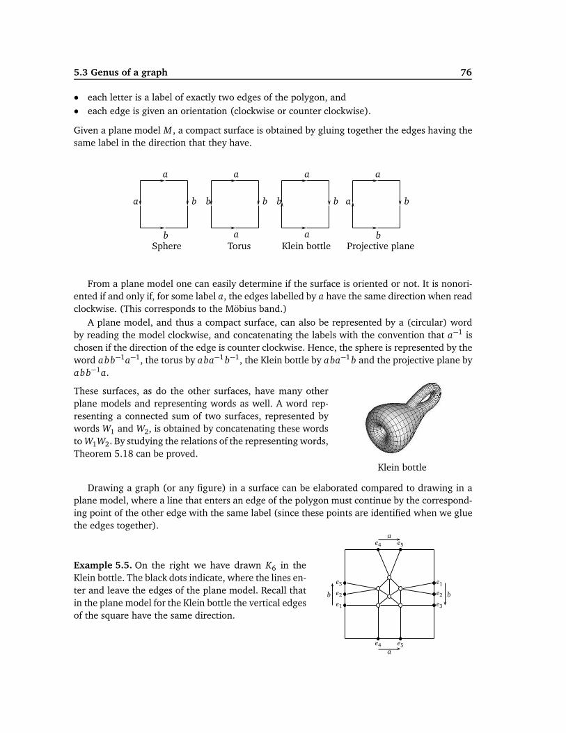
5.3 Genus of a graph 76
• each letter is a label of exactly two edges of the polygon, and• each edge is given an orientation (clockwise or counter clockwise).
Given a plane model M , a compact surface is obtained by gluing together the edges having thesame label in the direction that they have.
a
a
b
bSphere
b
a
b
a
Torus
b
a
b
a
Klein bottle
a
a
b
bProjective plane
From a plane model one can easily determine if the surface is oriented or not. It is nonori-ented if and only if, for some label a, the edges labelled by a have the same direction when readclockwise. (This corresponds to the Möbius band.)
A plane model, and thus a compact surface, can also be represented by a (circular) wordby reading the model clockwise, and concatenating the labels with the convention that a−1 ischosen if the direction of the edge is counter clockwise. Hence, the sphere is represented by theword abb−1a−1, the torus by aba−1 b−1, the Klein bottle by aba−1 b and the projective plane byabb−1a.
These surfaces, as do the other surfaces, have many otherplane models and representing words as well. A word rep-resenting a connected sum of two surfaces, represented bywords W1 and W2, is obtained by concatenating these wordsto W1W2. By studying the relations of the representing words,Theorem 5.18 can be proved.
Klein bottle
Drawing a graph (or any figure) in a surface can be elaborated compared to drawing in aplane model, where a line that enters an edge of the polygon must continue by the correspond-ing point of the other edge with the same label (since these points are identified when we gluethe edges together).
Example 5.5. On the right we have drawn K6 in theKlein bottle. The black dots indicate, where the lines en-ter and leave the edges of the plane model. Recall thatin the plane model for the Klein bottle the vertical edgesof the square have the same direction.
b
a
b
a
e1
e2
e3
e4 e5
e1
e2
e3
e5e4
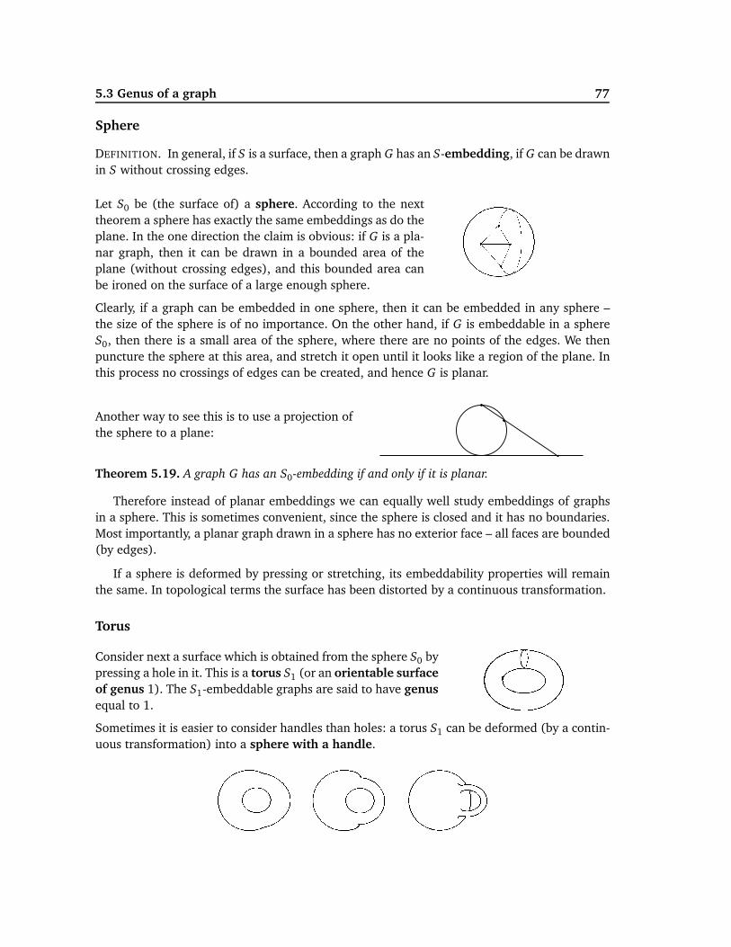
5.3 Genus of a graph 77
Sphere
DEFINITION. In general, if S is a surface, then a graph G has an S-embedding, if G can be drawnin S without crossing edges.
Let S0 be (the surface of) a sphere. According to the nexttheorem a sphere has exactly the same embeddings as do theplane. In the one direction the claim is obvious: if G is a pla-nar graph, then it can be drawn in a bounded area of theplane (without crossing edges), and this bounded area canbe ironed on the surface of a large enough sphere.
����Clearly, if a graph can be embedded in one sphere, then it can be embedded in any sphere –the size of the sphere is of no importance. On the other hand, if G is embeddable in a sphereS0, then there is a small area of the sphere, where there are no points of the edges. We thenpuncture the sphere at this area, and stretch it open until it looks like a region of the plane. Inthis process no crossings of edges can be created, and hence G is planar.
Another way to see this is to use a projection ofthe sphere to a plane:
Theorem 5.19. A graph G has an S0-embedding if and only if it is planar.
Therefore instead of planar embeddings we can equally well study embeddings of graphsin a sphere. This is sometimes convenient, since the sphere is closed and it has no boundaries.Most importantly, a planar graph drawn in a sphere has no exterior face – all faces are bounded(by edges).
If a sphere is deformed by pressing or stretching, its embeddability properties will remainthe same. In topological terms the surface has been distorted by a continuous transformation.
Torus
Consider next a surface which is obtained from the sphere S0 bypressing a hole in it. This is a torus S1 (or an orientable surfaceof genus 1). The S1-embeddable graphs are said to have genusequal to 1.
����Sometimes it is easier to consider handles than holes: a torus S1 can be deformed (by a contin-uous transformation) into a sphere with a handle.
���� ���� ����
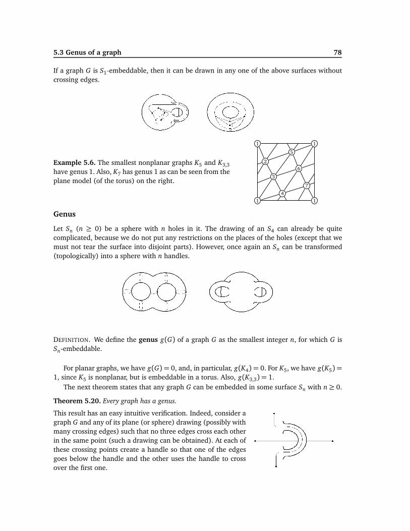
5.3 Genus of a graph 78
If a graph G is S1-embeddable, then it can be drawn in any one of the above surfaces withoutcrossing edges.
���� ����Example 5.6. The smallest nonplanar graphs K5 and K3,3
have genus 1. Also, K7 has genus 1 as can be seen from theplane model (of the torus) on the right.
1
1 1
1
2
3
4
5
6
7
Genus
Let Sn (n ≥ 0) be a sphere with n holes in it. The drawing of an S4 can already be quitecomplicated, because we do not put any restrictions on the places of the holes (except that wemust not tear the surface into disjoint parts). However, once again an Sn can be transformed(topologically) into a sphere with n handles.
������ ������DEFINITION. We define the genus g(G) of a graph G as the smallest integer n, for which G isSn-embeddable.
For planar graphs, we have g(G) = 0, and, in particular, g(K4) = 0. For K5, we have g(K5) =
1, since K5 is nonplanar, but is embeddable in a torus. Also, g(K3,3) = 1.The next theorem states that any graph G can be embedded in some surface Sn with n≥ 0.
Theorem 5.20. Every graph has a genus.
This result has an easy intuitive verification. Indeed, consider agraph G and any of its plane (or sphere) drawing (possibly withmany crossing edges) such that no three edges cross each otherin the same point (such a drawing can be obtained). At each ofthese crossing points create a handle so that one of the edgesgoes below the handle and the other uses the handle to crossover the first one.
������
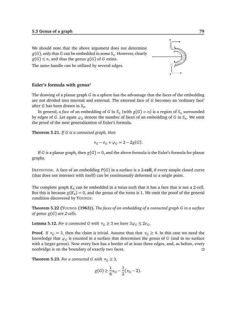
5.3 Genus of a graph 79
We should note that the above argument does not determineg(G), only that G can be embedded in some Sn. However, clearlyg(G) ≤ n, and thus the genus g(G) of G exists.
The same handle can be utilized by several edges.������
Euler’s formula with genus∗
The drawing of a planar graph G in a sphere has the advantage that the faces of the embeddingare not divided into internal and external. The external face of G becomes an ‘ordinary face’after G has been drawn in S0.
In general, a face of an embedding of G in Sn (with g(G) = n) is a region of Sn surroundedby edges of G. Let again ϕG denote the number of faces of an embedding of G in Sn. We omitthe proof of the next generalization of Euler’s formula.
Theorem 5.21. If G is a connected graph, then
νG − ǫG +ϕG = 2− 2g(G) .
If G is a planar graph, then g(G) = 0, and the above formula is the Euler’s formula for planargraphs.
DEFINITION. A face of an embedding P(G) in a surface is a 2-cell, if every simple closed curve(that does not intersect with itself) can be continuously deformed to a single point.
The complete graph K4 can be embedded in a torus such that it has a face that is not a 2-cell.But this is because g(K4) = 0, and the genus of the torus is 1. We omit the proof of the generalcondition discovered by YOUNGS:
Theorem 5.22 (YOUNGS (1963)). The faces of an embedding of a connected graph G in a surface
of genus g(G) are 2-cells.
Lemma 5.12. For a connected G with νG ≥ 3 we have 3ϕG ≤ 2ǫG.
Proof. If νG = 3, then the claim is trivial. Assume thus that νG ≥ 4. In this case we need theknowledge that ϕG is counted in a surface that determines the genus of G (and in no surfacewith a larger genus). Now every face has a border of at least three edges, and, as before, everynonbridge is on the boundary of exactly two faces. ⊓⊔
Theorem 5.23. For a connected G with νG ≥ 3,
g(G) ≥1
6ǫG −
1
2(νG − 2) .
5.3 Genus of a graph 80
Proof. By the previous lemma, 3ϕG ≤ 2ǫG, and by the generalized Euler’s formula, ϕG = ǫG −
νG + 2− 2g(G). Combining these we obtain that 3ǫG − 3νG + 6− 6g(G) ≤ 2ǫG, and the claimfollows. ⊓⊔
By this theorem, we can compute lower bounds for the genus g(G) without drawing anyembeddings. As an example, let G = K8. In this case νG = 8, ǫG = 28, and so g(G) ≥ 5
3 . Sincethe genus is always an integer, g(G) ≥ 2. We deduce that K8 cannot be embedded in the surfaceS1 of the torus.
If H ⊆ G, then clearly g(H) ≤ g(G), since H is obtained from G by omitting vertices andedges. In particular,
Lemma 5.13. For a graph G of order n, g(G) ≤ g(Kn).
For the complete graphs Kn a good lower bound was found early.
Theorem 5.24 (HEAWOOD (1890)). If n≥ 3, then
g(Kn) ≥(n− 3)(n− 4)
12.
Proof. The number of edges in Kn is equal to ǫG =12 n(n − 1). By Theorem 5.23, we obtain
g(Kn)≥ (1/6)ǫG − (1/2)(n− 2) = (1/12)(n− 3)(n− 4) . ⊓⊔
This result was dramatically improved to obtain
Theorem 5.25 (RINGEL AND YOUNGS (1968)). If n≥ 3, then
g(Kn) =
¡(n− 3)(n− 4)
12
¤.
Therefore g(K6) = ⌈3 · 2/12⌉= ⌈1/2⌉= 1. Also, g(K7) = 1, but g(K8) = 2.By Theorem 5.25,
Theorem 5.26. For all graphs G of order n≥ 3,
g(G) ≤
¡(n− 3)(n− 4)
12
¤.
Also, we know the exact genus for the complete bipartite graphs:
Theorem 5.27 ( RINGEL (1965)). For the complete bipartite graphs,
g(Km,n) =
¡(m− 2)(n− 2)
4
¤.
5.3 Genus of a graph 81
Chromatic numbers∗
For the planar graphs G, the proof of the 4-Colour Theorem, χ(G) ≤ 4, is extremely long anddifficult. This in mind, it is surprising that the generalization of the 4-Colour Theorem for genus≥ 1 is much easier. HEAWOOD proved a hundred years ago:
Theorem 5.28 (HEAWOOD). If g(G) = g ≥ 1, then
χ(G) ≤
�7+p
1+ 48g
2
�.
Notice that for g = 0 this theorem would be the 4-colour theorem. HEAWOOD proved it ‘only’for g ≥ 1.
Using the result of RINGEL AND YOUNGS and some elementary computations we can provethat the above theorem is the best possible.
Theorem 5.29. For each g ≥ 1, there exists a graph G with genus g(G) = g so that
χ(G) =
�7+p
1+ 48g
2
�.
If a nonplanar graph G can be embedded in a torus, then g(G) = 1, and χ(G) ≤ ⌊(7 +p1+ 48g)/2⌋= 7. Moreover, for G = K7 we have that χ(K7) = 7 and g(K7) = 1.
Three dimensions∗
Every graph can be drawn without crossing edges in the 3-dimensional space. Such a drawing iscalled spatial embedding of the graph. Indeed, such an embedding can be achieved by puttingall vertices of G on a line, and then drawing the edges in different planes that contain the line.Alternatively, the vertices of G can be put in a sphere, and drawing the edges as straight linescrossing the sphere inside.
A spatial embedding of a graph G is said to have linked cycles, if two cycles of G form alink (they cannot be separated in the space). By CONWAY and GORDON in 1983 every spatialembedding of K6 contains linked cycles.
It was shown by ROBERTSON, SEYMOUR AND THOMAS (1993) that there is a set of 7 graphssuch that a graph G has a spatial embedding without linked cycles if and only if G does nothave a minor belonging to this set.
This family of forbidden graphs was originally found by SACHS (without proof), and it con-tains K6 and the Petersen graph. Every graph in the set has 15 edges, which is curious.
For further results and proofs concerning graphs in surfaces, see
B. MOHAR AND C. THOMASSEN, “Graphs on Surfaces”, Johns Hopkins, 2001.
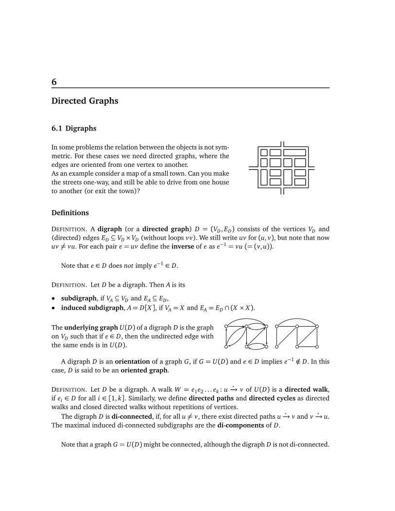
6
Directed Graphs
6.1 Digraphs
In some problems the relation between the objects is not sym-metric. For these cases we need directed graphs, where theedges are oriented from one vertex to another.As an example consider a map of a small town. Can you makethe streets one-way, and still be able to drive from one houseto another (or exit the town)?
Definitions
DEFINITION. A digraph (or a directed graph) D = (VD, ED) consists of the vertices VD and(directed) edges ED ⊆ VD×VD (without loops vv). We still write uv for (u, v), but note that nowuv 6= vu. For each pair e = uv define the inverse of e as e−1 = vu (= (v,u)).
Note that e ∈ D does not imply e−1 ∈ D.
DEFINITION. Let D be a digraph. Then A is its
• subdigraph, if VA ⊆ VD and EA ⊆ ED,• induced subdigraph, A= D[X ], if VA = X and EA = ED ∩ (X × X ).
The underlying graph U(D) of a digraph D is the graphon VD such that if e ∈ D, then the undirected edge withthe same ends is in U(D).
A digraph D is an orientation of a graph G, if G = U(D) and e ∈ D implies e−1 /∈ D. In thiscase, D is said to be an oriented graph.
DEFINITION. Let D be a digraph. A walk W = e1e2 . . . ek : u⋆−→ v of U(D) is a directed walk,
if ei ∈ D for all i ∈ [1, k]. Similarly, we define directed paths and directed cycles as directedwalks and closed directed walks without repetitions of vertices.
The digraph D is di-connected, if, for all u 6= v, there exist directed paths u⋆−→ v and v
⋆−→ u.
The maximal induced di-connected subdigraphs are the di-components of D.
Note that a graph G = U(D)might be connected, although the digraph D is not di-connected.
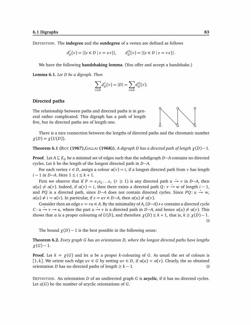
6.1 Digraphs 83
DEFINITION. The indegree and the outdegree of a vertex are defined as follows
d ID(v) = |{e ∈ D | e = x v}|, dO
D (v) = |{e ∈ D | e = v x}| .
We have the following handshaking lemma. (You offer and accept a handshake.)
Lemma 6.1. Let D be a digraph. Then
∑
v∈D
d ID(v) = |D|=∑
v∈D
dOD(v).
Directed paths
The relationship between paths and directed paths is in gen-eral rather complicated. This digraph has a path of lengthfive, but its directed paths are of length one.
There is a nice connection between the lengths of directed paths and the chromatic numberχ(D) = χ(U(D)).
Theorem 6.1 (ROY (1967),GALLAI (1968)). A digraph D has a directed path of length χ(D)−1.
Proof. Let A⊆ ED be a minimal set of edges such that the subdigraph D−A contains no directedcycles. Let k be the length of the longest directed path in D−A.
For each vertex v ∈ D, assign a colour α(v) = i, if a longest directed path from v has lengthi − 1 in D−A. Here 1≤ i ≤ k+ 1.
First we observe that if P = e1e2 . . . er (r ≥ 1) is any directed path u⋆−→ v in D−A, then
α(u) 6= α(v). Indeed, if α(v) = i, then there exists a directed path Q : v⋆−→ w of length i − 1,
and PQ is a directed path, since D−A does not contain directed cycles. Since PQ : u⋆−→ w,
α(u) 6= i = α(v). In particular, if e = uv ∈ D−A, then α(u) 6= α(v).Consider then an edge e = vu ∈ A. By the minimality of A, (D−A)+e contains a directed cycle
C : u⋆−→ v −→ u, where the part u
⋆−→ v is a directed path in D−A, and hence α(u) 6= α(v). This
shows that α is a proper colouring of U(D), and therefore χ(D)≤ k + 1, that is, k ≥ χ(D)− 1.⊓⊔
The bound χ(D)− 1 is the best possible in the following sense:
Theorem 6.2. Every graph G has an orientation D, where the longest directed paths have lengths
χ(G)− 1.
Proof. Let k = χ(G) and let α be a proper k-colouring of G. As usual the set of colours is[1, k]. We orient each edge uv ∈ G by setting uv ∈ D, if α(u) < α(v). Clearly, the so obtainedorientation D has no directed paths of length ≥ k− 1. ⊓⊔
DEFINITION. An orientation D of an undirected graph G is acyclic, if it has no directed cycles.Let a(G) be the number of acyclic orientations of G.
6.1 Digraphs 84
The next result is charming, since χG(−1) measures the number of proper colourings of G
using −1 colours!
Theorem 6.3 (STANLEY (1973)). Let G be a graph of order n. Then the number of the acyclic
orientations of G is
a(G) = (−1)nχG(−1) ,
where χG is the chromatic polynomial of G.
Proof. The proof is by induction on ǫG. First, if G is discrete, then χG(k) = kn, and a(G) = 1=(−1)n(−1)n = (−1)nχG(−1) as required.
Now χG(k) is a polynomial that satisfies the recurrence χG(k) = χG−e(k)−χG∗e(k). To provethe claim, we show that a(G) satisfies the same recurrence.
Indeed, ifa(G) = a(G−e) + a(G ∗ e) (6.1)
then, by the induction hypothesis,
a(G) = (−1)nχG−e(−1) + (−1)n−1χG∗e(−1) = (−1)nχG(−1) .
For (6.1), we observe that every acyclic orientation of G gives an acyclic orientation of G−e.On the other hand, if D is an acyclic orientation of G−e for e = uv, it extends to an acyclicorientation of G by putting e1 : u → v or e2 : v → u. Indeed, if D has no directed path u
⋆−→ v,
we choose e2, and if D has no directed path v⋆−→ u, we choose e1. Note that since D is acyclic,
it cannot have both ways u⋆−→ v and v
⋆−→ u.
We conclude that a(G) = a(G−e) + b, where b is the number of acyclic orientations D ofG−e that extend in both ways e1 and e2. The acyclic orientations D that extend in both waysare exactly those that contain
neither u⋆−→ v nor v
⋆−→ u as a directed path. (6.2)
Each acyclic orientation of G ∗ e corresponds in a natural way to an acyclic orientation D ofG−e that satisfies (6.2). Therefore b = a(G ∗ e), and the proof is completed. ⊓⊔
One-way traffic
Every graph can be oriented, but the result may not be di-connected. In the one-way trafficproblem the resulting orientation should be di-connected, for otherwise someone is not able todrive home. ROBBINS’ theorem solves this problem.
DEFINITION. A graph G is di-orientable, if there is a di-connected oriented graph D such thatG = U(D).
Theorem 6.4 (ROBBINS (1939)). A connected graph G is di-orientable if and only if G has no
bridges.
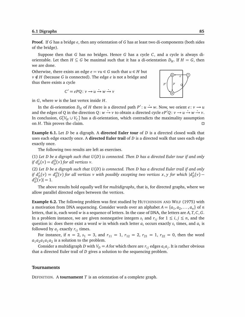
6.1 Digraphs 85
Proof. If G has a bridge e, then any orientation of G has at least two di-components (both sidesof the bridge).
Suppose then that G has no bridges. Hence G has a cycle C , and a cycle is always di-orientable. Let then H ⊆ G be maximal such that it has a di-orientation DH . If H = G, thenwe are done.
Otherwise, there exists an edge e = vu ∈ G such that u ∈ H butv /∈ H (because G is connected). The edge e is not a bridge andthus there exists a cycle
C ′ = ePQ : v −→ u⋆−→ w
⋆−→ v
in G, where w is the last vertex inside H.
w
u v
P
e
QP ′
In the di-orientation DH of H there is a directed path P ′ : u⋆−→ w. Now, we orient e : v −→ u
and the edges of Q in the direction Q : w⋆−→ v to obtain a directed cycle eP ′Q : v −→ u
⋆−→ w
⋆−→ v.
In conclusion, G[VH ∪ VC] has a di-orientation, which contradicts the maximality assumptionon H. This proves the claim. ⊓⊔
Example 6.1. Let D be a digraph. A directed Euler tour of D is a directed closed walk thatuses each edge exactly once. A directed Euler trail of D is a directed walk that uses each edgeexactly once.
The following two results are left as exercises.
(1) Let D be a digraph such that U(D) is connected. Then D has a directed Euler tour if and only
if d ID(v) = dO
D (v) for all vertices v.
(2) Let D be a digraph such that U(D) is connected. Then D has a directed Euler trail if and only
if d ID(v) = dO
D (v) for all vertices v with possibly excepting two vertices x , y for which |d ID(v) −
dOD (v)|= 1.
The above results hold equally well for multidigraphs, that is, for directed graphs, where weallow parallel directed edges between the vertices.
Example 6.2. The following problem was first studied by HUTCHINSON AND WILF (1975) witha motivation from DNA sequencing. Consider words over an alphabet A= {a1, a2, . . . , an} of n
letters, that is, each word w is a sequence of letters. In the case of DNA, the letters are A, T, C , G.In a problem instance, we are given nonnegative integers si and ri j for 1 ≤ i, j ≤ n, and thequestion is: does there exist a word w in which each letter ai occurs exactly si times, and ai isfollowed by a j exactly ri j times.
For instance, if n = 2, s1 = 3, and r11 = 1, r12 = 2, r21 = 1, r22 = 0, then the worda1a2a1a1a2 is a solution to the problem.
Consider a multidigraph D with VD = A for which there are ri j edges aia j. It is rather obviousthat a directed Euler trail of D gives a solution to the sequencing problem.
Tournaments
DEFINITION. A tournament T is an orientation of a complete graph.
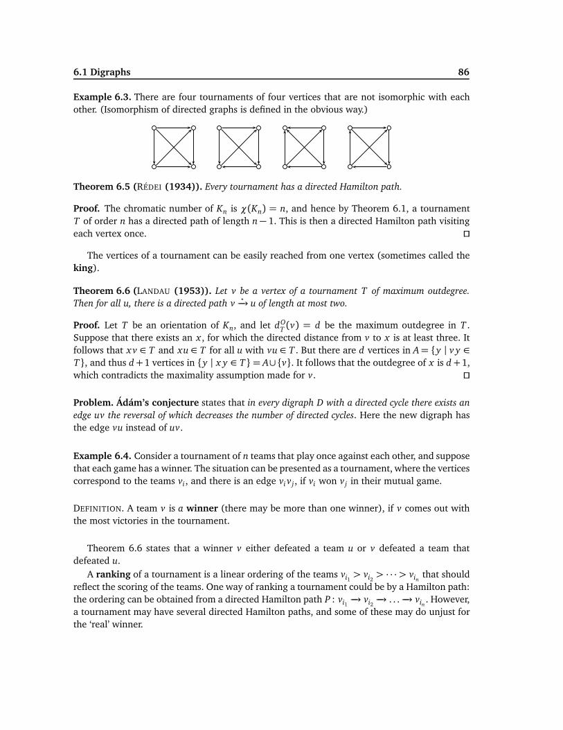
6.1 Digraphs 86
Example 6.3. There are four tournaments of four vertices that are not isomorphic with eachother. (Isomorphism of directed graphs is defined in the obvious way.)
Theorem 6.5 (RÉDEI (1934)). Every tournament has a directed Hamilton path.
Proof. The chromatic number of Kn is χ(Kn) = n, and hence by Theorem 6.1, a tournamentT of order n has a directed path of length n− 1. This is then a directed Hamilton path visitingeach vertex once. ⊓⊔
The vertices of a tournament can be easily reached from one vertex (sometimes called theking).
Theorem 6.6 (LANDAU (1953)). Let v be a vertex of a tournament T of maximum outdegree.
Then for all u, there is a directed path v⋆−→ u of length at most two.
Proof. Let T be an orientation of Kn, and let dOT(v) = d be the maximum outdegree in T .
Suppose that there exists an x , for which the directed distance from v to x is at least three. Itfollows that x v ∈ T and xu ∈ T for all u with vu ∈ T . But there are d vertices in A= {y | v y ∈
T}, and thus d+1 vertices in {y | x y ∈ T}= A∪{v}. It follows that the outdegree of x is d +1,which contradicts the maximality assumption made for v. ⊓⊔
Problem. Ádám’s conjecture states that in every digraph D with a directed cycle there exists an
edge uv the reversal of which decreases the number of directed cycles. Here the new digraph hasthe edge vu instead of uv.
Example 6.4. Consider a tournament of n teams that play once against each other, and supposethat each game has a winner. The situation can be presented as a tournament, where the verticescorrespond to the teams vi, and there is an edge vi v j, if vi won v j in their mutual game.
DEFINITION. A team v is a winner (there may be more than one winner), if v comes out withthe most victories in the tournament.
Theorem 6.6 states that a winner v either defeated a team u or v defeated a team thatdefeated u.
A ranking of a tournament is a linear ordering of the teams vi1> vi2
> · · ·> vinthat should
reflect the scoring of the teams. One way of ranking a tournament could be by a Hamilton path:the ordering can be obtained from a directed Hamilton path P : vi1
−→ vi2−→ . . . −→ vin
. However,a tournament may have several directed Hamilton paths, and some of these may do unjust forthe ‘real’ winner.
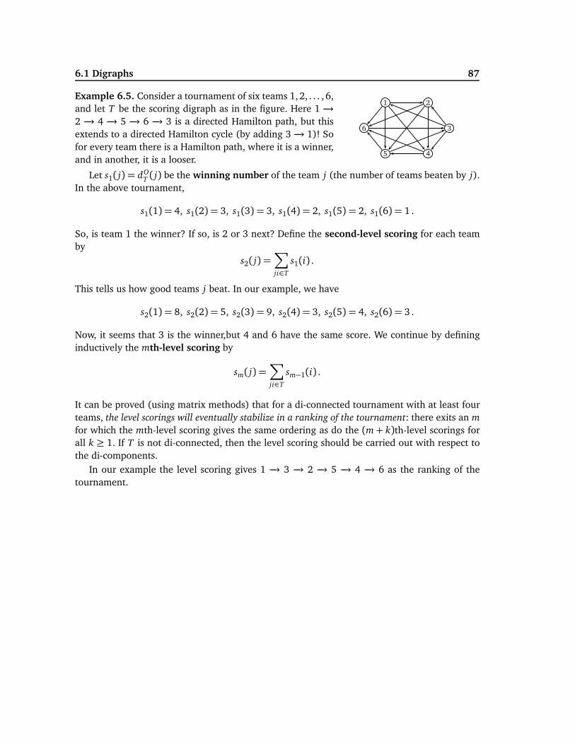
6.1 Digraphs 87
Example 6.5. Consider a tournament of six teams 1,2, . . . , 6,and let T be the scoring digraph as in the figure. Here 1 −→2 −→ 4 −→ 5 −→ 6 −→ 3 is a directed Hamilton path, but thisextends to a directed Hamilton cycle (by adding 3 −→ 1)! Sofor every team there is a Hamilton path, where it is a winner,and in another, it is a looser.
6
5
1
4
2
3
Let s1( j) = dOT ( j) be the winning number of the team j (the number of teams beaten by j).
In the above tournament,
s1(1) = 4, s1(2) = 3, s1(3) = 3, s1(4) = 2, s1(5) = 2, s1(6) = 1 .
So, is team 1 the winner? If so, is 2 or 3 next? Define the second-level scoring for each teamby
s2( j) =∑
ji∈T
s1(i) .
This tells us how good teams j beat. In our example, we have
s2(1) = 8, s2(2) = 5, s2(3) = 9, s2(4) = 3, s2(5) = 4, s2(6) = 3 .
Now, it seems that 3 is the winner,but 4 and 6 have the same score. We continue by defininginductively the mth-level scoring by
sm( j) =∑
ji∈T
sm−1(i) .
It can be proved (using matrix methods) that for a di-connected tournament with at least fourteams, the level scorings will eventually stabilize in a ranking of the tournament: there exits an m
for which the mth-level scoring gives the same ordering as do the (m+ k)th-level scorings forall k ≥ 1. If T is not di-connected, then the level scoring should be carried out with respect tothe di-components.
In our example the level scoring gives 1 −→ 3 −→ 2 −→ 5 −→ 4 −→ 6 as the ranking of thetournament.
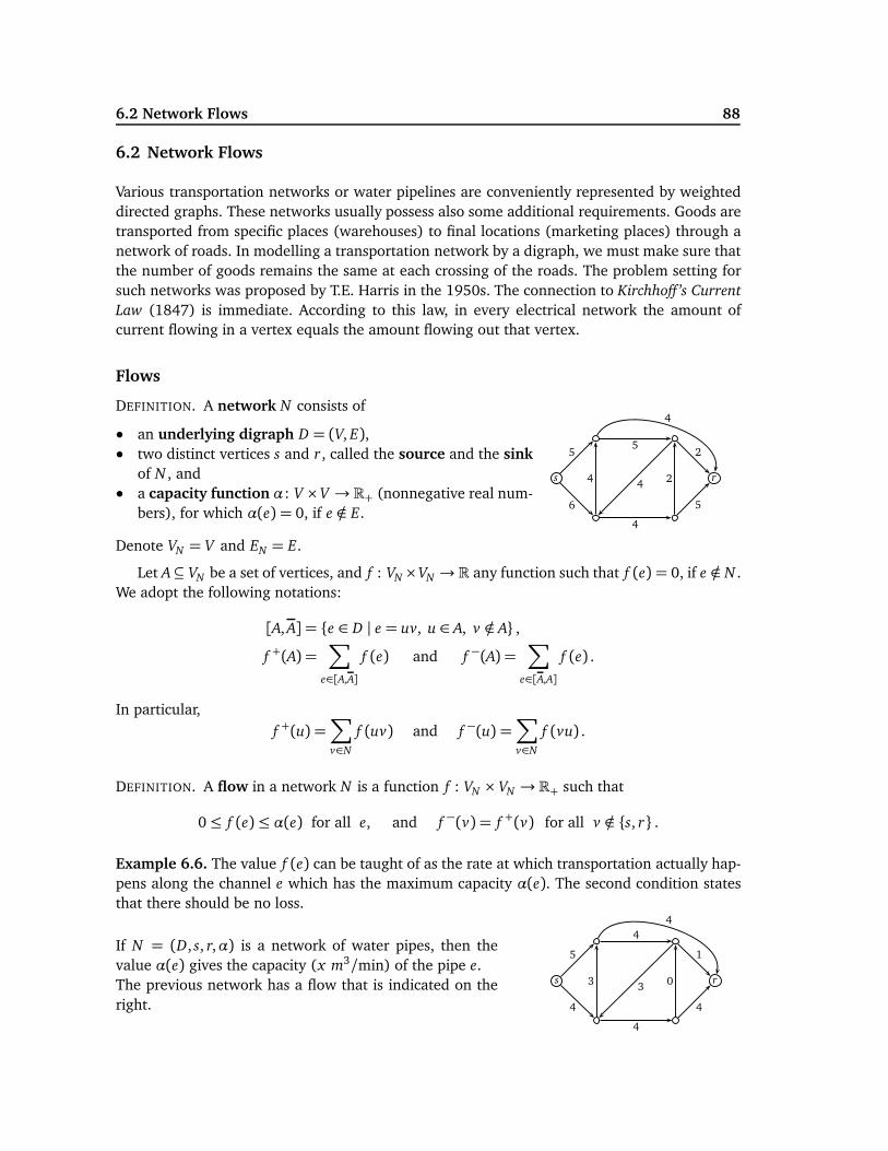
6.2 Network Flows 88
6.2 Network Flows
Various transportation networks or water pipelines are conveniently represented by weighteddirected graphs. These networks usually possess also some additional requirements. Goods aretransported from specific places (warehouses) to final locations (marketing places) through anetwork of roads. In modelling a transportation network by a digraph, we must make sure thatthe number of goods remains the same at each crossing of the roads. The problem setting forsuch networks was proposed by T.E. Harris in the 1950s. The connection to Kirchhoff ’s Current
Law (1847) is immediate. According to this law, in every electrical network the amount ofcurrent flowing in a vertex equals the amount flowing out that vertex.
Flows
DEFINITION. A network N consists of
• an underlying digraph D = (V, E),• two distinct vertices s and r, called the source and the sink
of N , and• a capacity function α: V ×V → R+ (nonnegative real num-
bers), for which α(e) = 0, if e /∈ E.
Denote VN = V and EN = E.
s r
6
5
4
4
5
2
5
2
4
4
Let A⊆ VN be a set of vertices, and f : VN ×VN → R any function such that f (e) = 0, if e /∈ N .We adopt the following notations:
[A,A] = {e ∈ D | e = uv, u ∈ A, v /∈ A} ,
f +(A) =∑
e∈[A,A]
f (e) and f −(A) =∑
e∈[A,A]
f (e) .
In particular,f +(u) =∑
v∈N
f (uv) and f −(u) =∑
v∈N
f (vu) .
DEFINITION. A flow in a network N is a function f : VN × VN → R+ such that
0≤ f (e) ≤ α(e) for all e, and f −(v) = f +(v) for all v /∈ {s, r} .
Example 6.6. The value f (e) can be taught of as the rate at which transportation actually hap-pens along the channel e which has the maximum capacity α(e). The second condition statesthat there should be no loss.
If N = (D, s, r,α) is a network of water pipes, then thevalue α(e) gives the capacity (x m3/min) of the pipe e.The previous network has a flow that is indicated on theright.
s r
4
5
3
4
4
0
4
1
3
4
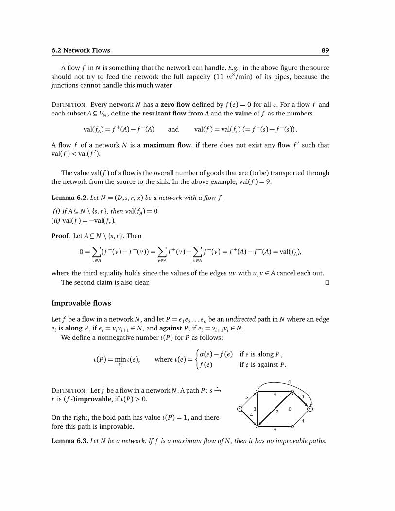
6.2 Network Flows 89
A flow f in N is something that the network can handle. E.g., in the above figure the sourceshould not try to feed the network the full capacity (11 m3/min) of its pipes, because thejunctions cannot handle this much water.
DEFINITION. Every network N has a zero flow defined by f (e) = 0 for all e. For a flow f andeach subset A⊆ VN , define the resultant flow from A and the value of f as the numbers
val( fA) = f +(A)− f −(A) and val( f ) = val( fs) (= f +(s)− f −(s)) .
A flow f of a network N is a maximum flow, if there does not exist any flow f ′ such thatval( f )< val( f ′).
The value val( f ) of a flow is the overall number of goods that are (to be) transported throughthe network from the source to the sink. In the above example, val( f ) = 9.
Lemma 6.2. Let N = (D, s, r,α) be a network with a flow f .
(i) If A⊆ N \ {s, r}, then val( fA) = 0.
(ii) val( f ) = −val( fr ).
Proof. Let A⊆ N \ {s, r}. Then
0=∑
v∈A
( f +(v)− f −(v)) =∑
v∈A
f +(v)−∑
v∈A
f −(v) = f +(A)− f −(A) = val( fA),
where the third equality holds since the values of the edges uv with u, v ∈ A cancel each out.The second claim is also clear. ⊓⊔
Improvable flows
Let f be a flow in a network N , and let P = e1e2 . . . en be an undirected path in N where an edgeei is along P, if ei = vi vi+1 ∈ N , and against P, if ei = vi+1vi ∈ N .
We define a nonnegative number ι(P) for P as follows:
ι(P) =minei
ι(e), where ι(e) =
¨α(e)− f (e) if e is along P ,
f (e) if e is against P.
DEFINITION. Let f be a flow in a network N . A path P : s⋆−→
r is ( f -)improvable, if ι(P) > 0.
On the right, the bold path has value ι(P) = 1, and there-fore this path is improvable.
s r
5
3
4
4
0
4
4
43
1
Lemma 6.3. Let N be a network. If f is a maximum flow of N, then it has no improvable paths.
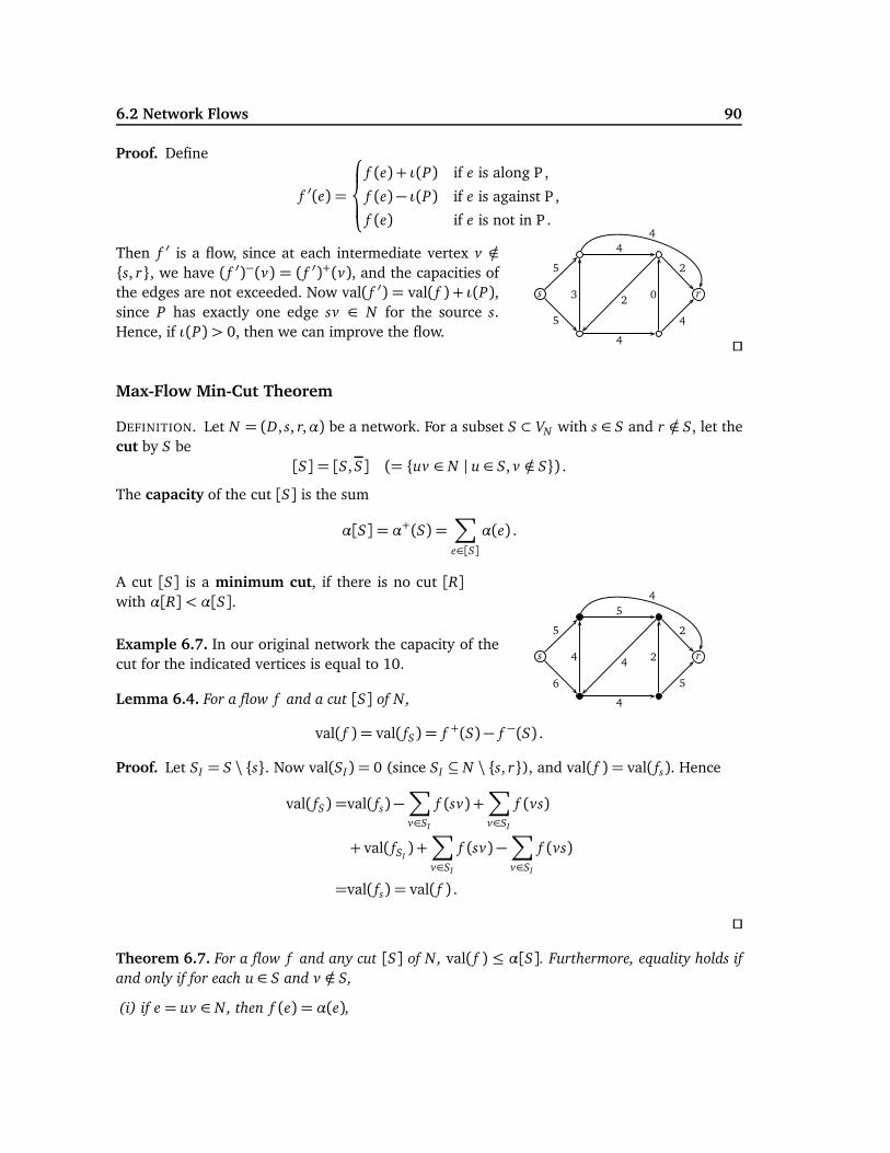
6.2 Network Flows 90
Proof. Define
f ′(e) =
f (e) + ι(P) if e is along P ,
f (e)− ι(P) if e is against P ,
f (e) if e is not in P .
Then f ′ is a flow, since at each intermediate vertex v /∈
{s, r}, we have ( f ′)−(v) = ( f ′)+(v), and the capacities ofthe edges are not exceeded. Now val( f ′) = val( f ) + ι(P),since P has exactly one edge sv ∈ N for the source s.Hence, if ι(P) > 0, then we can improve the flow.
s r
5
3
4
4
0
4
4
5
2
2
⊓⊔
Max-Flow Min-Cut Theorem
DEFINITION. Let N = (D, s, r,α) be a network. For a subset S ⊂ VN with s ∈ S and r /∈ S, let thecut by S be
[S] = [S,S] (= {uv ∈ N | u ∈ S, v /∈ S}) .
The capacity of the cut [S] is the sum
α[S] = α+(S) =∑
e∈[S]
α(e) .
A cut [S] is a minimum cut, if there is no cut [R]with α[R] < α[S].
Example 6.7. In our original network the capacity of thecut for the indicated vertices is equal to 10.
s r
5
4
4
5
2
56
4
2
4
Lemma 6.4. For a flow f and a cut [S] of N,
val( f ) = val( fS) = f +(S)− f −(S) .
Proof. Let SI = S \ {s}. Now val(SI) = 0 (since SI ⊆ N \ {s, r}), and val( f ) = val( fs). Hence
val( fS) =val( fs)−∑
v∈SI
f (sv) +∑
v∈SI
f (vs)
+ val( fSI) +∑
v∈SI
f (sv)−∑
v∈SI
f (vs)
=val( fs) = val( f ) .
⊓⊔
Theorem 6.7. For a flow f and any cut [S] of N, val( f ) ≤ α[S]. Furthermore, equality holds if
and only if for each u ∈ S and v /∈ S,
(i) if e = uv ∈ N, then f (e) = α(e),
6.2 Network Flows 91
(ii) if e = vu ∈ N, then f (e) = 0.
Proof. By the definition of a flow,
f +(S) =∑
e∈[S]
f (e) ≤∑
e∈[S]
α(e) = α[S] ,
and f −(S) ≥ 0. By Lemma 6.4, val( f ) = val( fS) = f +(S)− f −(S), and hence val( f ) ≤ α[S], asrequired. Also, the equality val( f ) = α[S] holds if and only if
(1) f +(S) = α[S] and (2) f −(S) = 0. This holds if and only if f (e) = α(e) for all e ∈ [S] (sincef (e) ≤ α(e)), and
(2) f (e) = 0 for all e = vu with u ∈ S, v /∈ S.
This proves the claim. ⊓⊔
In particular, if f is a maximum flow and [S] a minimum cut, then
val( f )≤ α[S] .
Corollary 6.1. If f is a flow and [S] a cut such that val( f ) = α[S], then f is a maximum flow
and [S] a minimum cut.
The following main result of network flows was proved independently by ELIAS, FEINSTEIN,SHANNON, by FORD AND FULKERSON, and by ROBACKER in 1955 – 56. The present approach isdue to Ford and Fulkerson.
Theorem 6.8. A flow f of a network N is maximum if and only if there are no f -improvable paths
in N.
Proof. By Lemma 6.3, a maximum flow cannot have improvable paths.Conversely, assume that N contains no f -improvable paths, and let
SI = {u ∈ N | for some path P : s⋆−→ u, ι(P) > 0} .
Set S = SI ∪ {s}.Consider an edge e = uv ∈ N , where u ∈ S and v /∈ S. Since u ∈ S, there exists a path
P : s⋆−→ u with ι(P) > 0. Moreover, since v /∈ S, ι(Pe) = 0 for the path Pe : s
⋆−→ v. Therefore
ι(e) = 0, and so f (e) = α(e).By the same argument, for an edge e = vu ∈ N with v /∈ S and u ∈ S, f (e) = 0.By Theorem 6.7, we have val( f ) = α[S]. Corollary 6.1 implies now that f is a maximum
flow (and [S] is a minimum cut). ⊓⊔
Theorem 6.9. Let N be a network, where the capacity function α: V × V → N has integer values.
Then N has a maximum flow with integer values.
Proof. Let f0 be the zero flow, f0(e) = 0 for all e ∈ V ×V . A maximum flow is constructed usingLemma 6.3 by increasing and decreasing the values of the edges by integers only. ⊓⊔
6.2 Network Flows 92
The proof of Theorem 6.8 showed also
Theorem 6.10 (Max-Flow Min-Cut). In a network N, the value val( f ) of a maximum flow equals
the capacity α[S] of a minimum cut.
Applications to graphs⋆
The Max-Flow Min-Cut Theorem is a strong result, and many of our previous results followfrom it.
We mention a connection to the Marriage Theorem, Theorem 3.9. For this, let G be a bipartitegraph with a bipartition (X , Y ), and consider a network N with vertices {s, r} ∪ X ∪ Y . Let theedges (with their capacities) be sx ∈ N (α(sx) = 1), yr ∈ N (α(yr) = 1) for all x ∈ X , y ∈ Y
together with the edges x y ∈ N (α(x y) = |X |+ 1), if x y ∈ G for x ∈ X , y ∈ Y . Then G has amatching that saturates X if and only if N has a maximum flow of value |X |. Now Theorem 6.10gives Theorem 3.9.
Next we apply the theorem to unit networks, where the capacities of the edges are equalto one (α(e) = 1 for all e ∈ N). We obtain results for (directed) graphs.
Lemma 6.5. Let N be a unit network with source s and sink r.
(i) The value val( f ) of a maximum flow equals the maximum number of edge-disjoint directed
paths s⋆−→ r.
(ii) The capacity of a minimum cut [S] equals the minimum number of edges whose removal de-
stroys the directed connections s⋆−→ r from s to r.
Proof. Exercise. ⊓⊔
Corollary 6.2. Let u and v be two vertices of a digraph D. The maximum number of edge-disjoint
directed paths u⋆−→ v equals the minimum number of edges, whose removal destroys all the directed
connections u⋆−→ v from D.
Proof. A network N with source s and sink r is obtained by setting the capacities equal to 1.The claim follows from Lemma 6.5 and Corollary 6.10. ⊓⊔
Corollary 6.3. Let u and v be two vertices of a graph G. The maximum number of edge-disjoint
paths u⋆−→ v equals the minimum number of edges, whose removal destroys all the connections
u⋆−→ v from G.
Proof. Consider the digraph D that is obtained from G by replacing each (undirected) edge uv ∈
G by two directed edges uv ∈ D and vu ∈ D. The claim follows then easily from Corollary 6.2.⊓⊔
The next corollary is Menger’s Theorem for edge connectivity.
Corollary 6.4. A graph G is k-edge connected if and only if any two distinct vertices of G are
connected by at least k independent paths.
Proof. The claim follows immediately from Corollary 6.3. ⊓⊔
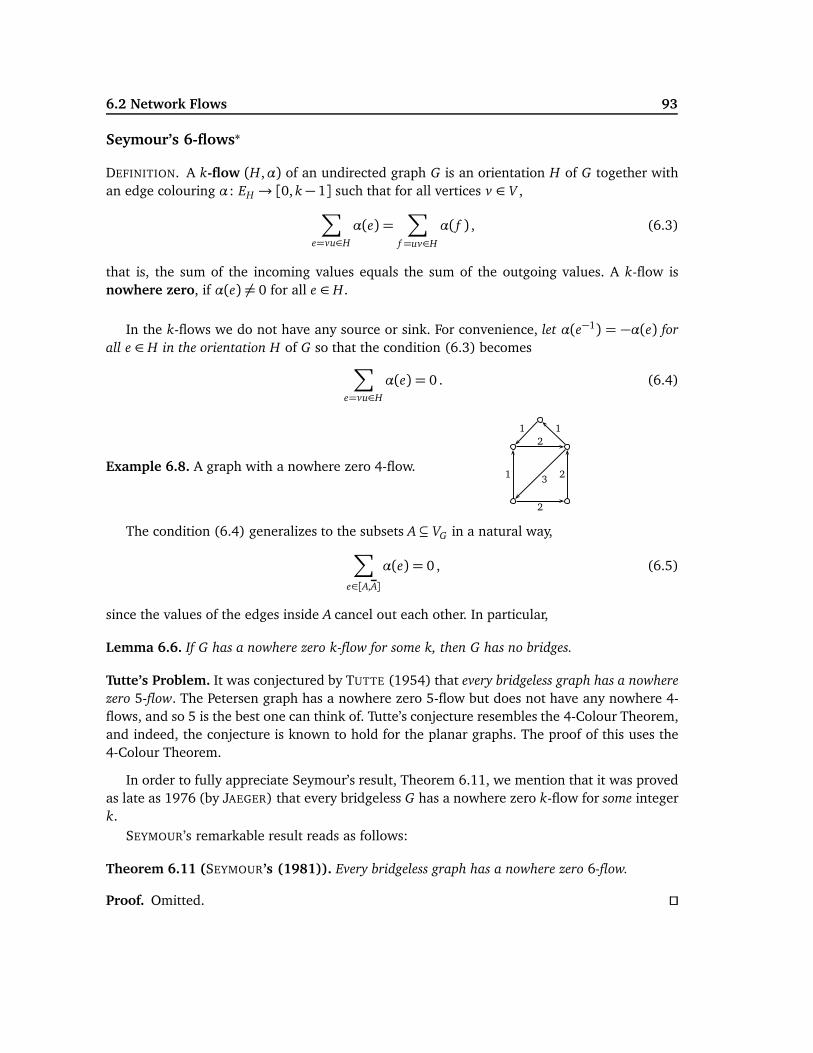
6.2 Network Flows 93
Seymour’s 6-flows∗
DEFINITION. A k-flow (H,α) of an undirected graph G is an orientation H of G together withan edge colouring α: EH → [0, k − 1] such that for all vertices v ∈ V ,
∑
e=vu∈H
α(e) =∑
f=uv∈H
α( f ) , (6.3)
that is, the sum of the incoming values equals the sum of the outgoing values. A k-flow isnowhere zero, if α(e) 6= 0 for all e ∈ H.
In the k-flows we do not have any source or sink. For convenience, let α(e−1) = −α(e) for
all e ∈ H in the orientation H of G so that the condition (6.3) becomes∑
e=vu∈H
α(e) = 0 . (6.4)
Example 6.8. A graph with a nowhere zero 4-flow.1
2
2
2
1
3
1
The condition (6.4) generalizes to the subsets A⊆ VG in a natural way,∑
e∈[A,A]
α(e) = 0 , (6.5)
since the values of the edges inside A cancel out each other. In particular,
Lemma 6.6. If G has a nowhere zero k-flow for some k, then G has no bridges.
Tutte’s Problem. It was conjectured by TUTTE (1954) that every bridgeless graph has a nowhere
zero 5-flow. The Petersen graph has a nowhere zero 5-flow but does not have any nowhere 4-flows, and so 5 is the best one can think of. Tutte’s conjecture resembles the 4-Colour Theorem,and indeed, the conjecture is known to hold for the planar graphs. The proof of this uses the4-Colour Theorem.
In order to fully appreciate Seymour’s result, Theorem 6.11, we mention that it was provedas late as 1976 (by JAEGER) that every bridgeless G has a nowhere zero k-flow for some integerk.
SEYMOUR’s remarkable result reads as follows:
Theorem 6.11 (SEYMOUR’s (1981)). Every bridgeless graph has a nowhere zero 6-flow.
Proof. Omitted. ⊓⊔
6.2 Network Flows 94
DEFINITION. The flow number f (G) of a bridgeless graph G is the least integer k for which G
has a nowhere zero k-flow.
Theorem 6.12. A connected graph G has a flow number f (G) = 2 if and only if it is eulerian.
Proof. Suppose G is eulerian, and consider an Euler tour W of G. Let D be the orientation ofG corresponding to the direction of W . If an edge uv ∈ D, let α(e) = 1. Since W arrives andleaves each vertex equally many times, the function α is a nowhere zero 2-flow.
Conversely, let α be a nowhere zero 2-flow of an orientation D of G. Then necessarily thedegrees of the vertices are even, and so G is eulerian. ⊓⊔
Example 6.9. For each 3-regular bipartite graph G, we have f (G) ≤ 3. Indeed, let G be (X , Y )-bipartite. By Corollary 3.1, a 3-regular graph has a perfect matching M . Orient the edges e ∈ M
from X to Y , and set α(e) = 2. Orient the edges e /∈ M from Y to X , and set α(e) = 1. Since eachx ∈ X has exactly one neighbour y1 ∈ Y such that x y1 ∈ M , and two neighbours y2, y3 ∈ Y
such that x y2, x y3 /∈ M , we have that f (G) ≤ 3.
Theorem 6.13. We have f (K4) = 4, and if n> 4, then
f (Kn) =
¨2 if n is odd ,
3 if n is even .
Proof. Exercise. ⊓⊔
Index
N P-complete problems, 32-sets, 4
acyclic, 18digraph, 83
addressable, 22adjacency matrix, 6adjacent, 4augmented path, 35available colour, 42, 52
bipartite, 16bond, 24boundary, 61bridge, 18
capacity, 90capacity function, 88choosable, 70chromatic number χ(G), 52chromatic polynomial χG , 56closed walk, 12colouring, 52complement G, 10complete bipartite Km,k, 16complete graph Kn, 10connected, 24connected (component), 13connected sum, 75connectivity number κ(G), 24contracted vertex, 57critical, 53crossing number, 67cube, 11cut (in a network), 90cut vertex, 23cycle, 12
degree dG(v), 7
di-connected di-component, 82di-orientable, 84digraph, 82directed
Euler tour, trail, 85walk, path, cycle, 82
directed graphs (digraph), 5disconnected, 13disconnecting set, 27discrete graph, 10disjoint walks, 12distance, 13distance function, 5
edge, 4edge chromatic number χ ′(G), 42edge colouring, 5, 42edge cut, 24embedding, 77end (of a path), 12end (of an edge), 4Euler trail , tour, 29Euler’s formula, 62eulerian, 29even component, 38even cycle, 12exterior: face, boundary,vertex,edge, 61
face, 61fan, 28flow, 88flow number, 94forest, 18
genus, 78graph, 4graphical sequence, 9
Hamilton path, cycle, 31
Index 96
hamiltonian, 31Hamming distance, 22homeomorphic, 74
improvable (path), 89improvement (colouring), 43incident colours, 42indegree, 83independent paths, 12induced subdigraph, 82induced subgraph, 8interior: face, vertex, edge, 61intersection graph, 6inverse pair, 82inverse walk (path), 12isolated vertex, 7isomorphic, 5
join of walks, 12
king, 86kiss (circles), 72Kuratowski graph, 64
latin rectangle, 38latin square, 38leaf, 7line segment graph, 72linked cycles, 81list chromatic number, 70list colouring, 70loop, 4
Möbius band, 75map, 68matching, 35maximal planar graph, 63maximum
degree ∆(G), 7flow, 89matching, 35
minimumcut, 90degree δ(G), 7weighted distance, 13
minor, 73monochromatic, 48multigraph, 4
near-triangulation, 71neighbour, 4neighbourhood NG(v), 7network, 88nontrivial graph, 10
odd component, 38odd cycle, 12optimal colouring, 43order νG , 4orientable surface, 75orientation, 82oriented, 75oriented graph, 82outdegree, 83
parallel edges, 4partition, 3path, 12perfect matching, 35Petersen graph, 11, 32planar graph, 60plane embedding, 60plane model, 75proper colouring, 42, 52
Ramsey number, 48ranking, 86regular graph, 10resultant flow, 89
same parity, 3saturate (matching), 35separates, 23separating set, 23Shannon’s switching game, 20sink and source, 88size ǫG , 4spanning subgraph, 8spanning tree, 20spatial embedding, 81sphere, 77sphere with a handle, 77stable matching, 40stable set, 16subdigraph, 82subdivision, 60subgraph, 8surface, 75symmetric difference, 3
topologically equivalent, 74torus, 77tournament, 85trail, 29transversal, 37tree, 18triangle, 75triangle-free, 52triangulation, 75trivial graph, 10
Index 97
trivial path, 122-cell, 792-switch, 9
underlying digraph, 88underlying graph, 82unit networks, 92
vertex, 4
vertex colouring, 5
walk, 11weight, 13weight function, 5wheel, 51winning number, 87
zero flow, 89