A Primer on Graph Theory - Centro di Ricerca Matematica ...crm.sns.it/media/course/1518/murray-graphtheory.pdf · A Primer on Graph Theory Richard M. Murray Control and Dynamical

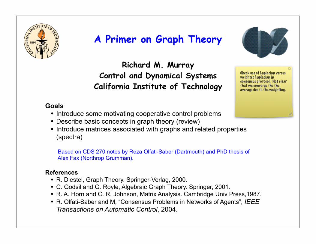
A Primer on Graph Theory

Richard M. MurrayControl and Dynamical Systems

California Institute of Technology

Goals• Introduce some motivating cooperative control problems• Describe basic concepts in graph theory (review)• Introduce matrices associated with graphs and related properties

(spectra)

Based on CDS 270 notes by Reza Olfati-Saber (Dartmouth) and PhD thesis of Alex Fax (Northrop Grumman).

References• R. Diestel, Graph Theory. Springer-Verlag, 2000. • C. Godsil and G. Royle, Algebraic Graph Theory. Springer, 2001. • R. A. Horn and C. R. Johnson, Matrix Analysis. Cambridge Univ Press,1987. • R. Olfati-Saber and M, “Consensus Problems in Networks of Agents”, IEEE

Transactions on Automatic Control, 2004.

Check use of Laplacian versus weighted Laplacian in consensus protocol. Not clear that we converge the the average due to the weighting.

Richard M. Murray, Caltech CDSCRM, Dec 07

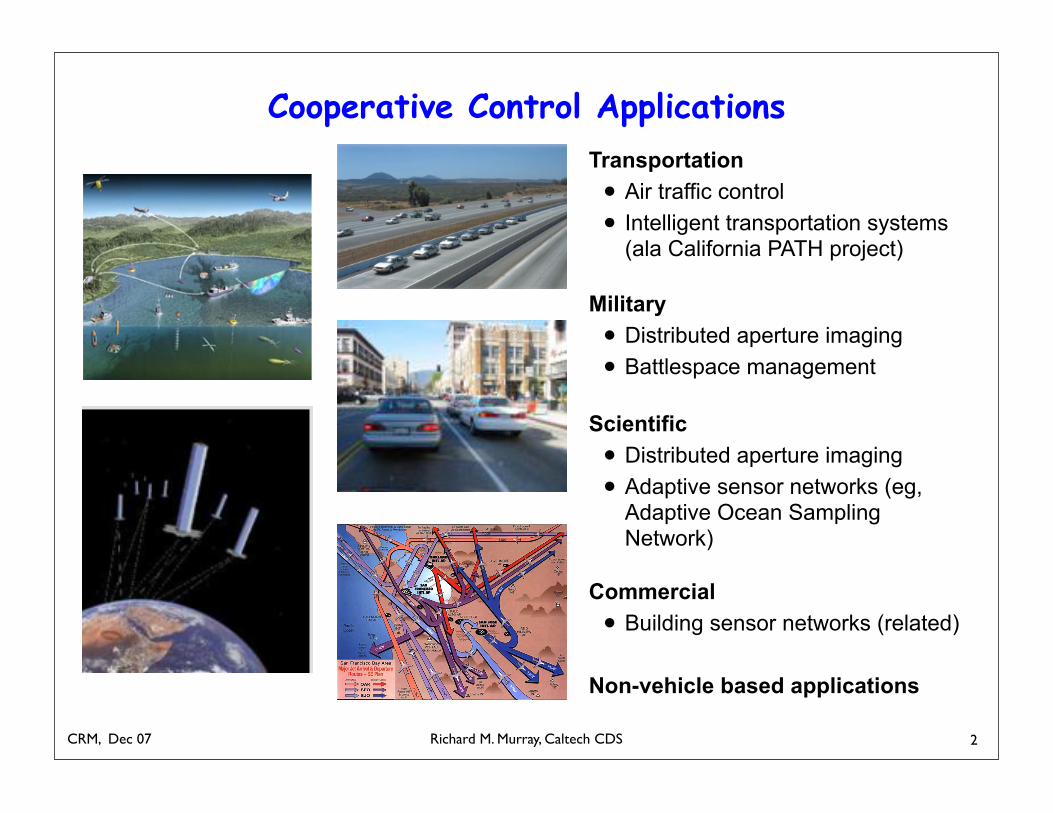
Cooperative Control ApplicationsTransportation• Air traffic control• Intelligent transportation systems

(ala California PATH project)

Military• Distributed aperture imaging• Battlespace management

Scientific• Distributed aperture imaging• Adaptive sensor networks (eg,

Adaptive Ocean Sampling Network)

Commercial• Building sensor networks (related)

Non-vehicle based applications

2

Richard M. Murray, Caltech CDSCRM, Dec 07 3

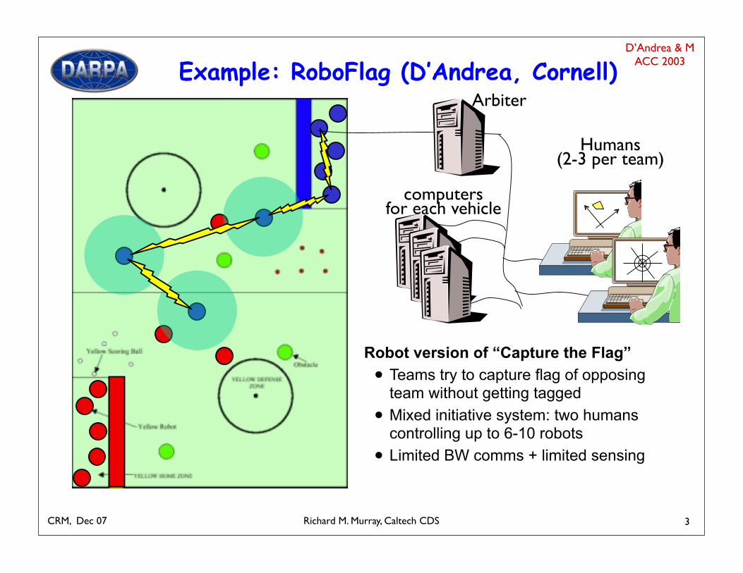
Arbiter

computersfor each vehicle

Humans(2-3 per team)

Example: RoboFlag (D’Andrea, Cornell)

Robot version of “Capture the Flag”• Teams try to capture flag of opposing

team without getting tagged• Mixed initiative system: two humans

controlling up to 6-10 robots• Limited BW comms + limited sensing

D’Andrea & MACC 2003


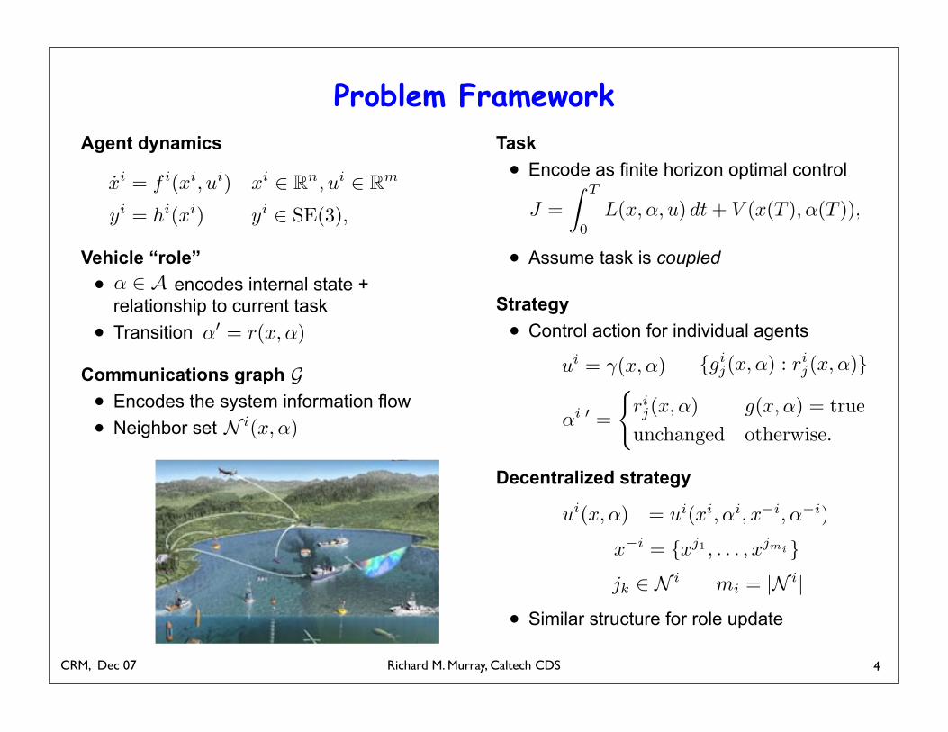
Problem FrameworkAgent dynamics

Vehicle “role”• encodes internal state +

relationship to current task

• Transition

Communications graph• Encodes the system information flow

• Neighbor set

Task• Encode as finite horizon optimal control

• Assume task is coupled

Strategy• Control action for individual agents

Decentralized strategy

• Similar structure for role update

4

N i(x,!)

J =! T

0L(x,!, u) dt + V (x(T ),!(T )),

ui = !(x,") {gij(x,!) : ri

j(x,!)}

!i ! =

!rij(x,!) g(x,!) = true

unchanged otherwise.

x!i = {xj1 , . . . , xjmi}

jk ! N i mi = |N i|

! ! A

!! = r(x,!)

G

ui(x,!) = ui(xi,!i, x!i,!!i)

xi = f i(xi, ui) xi ! Rn, ui ! Rm

yi = hi(xi) yi ! SE(3),


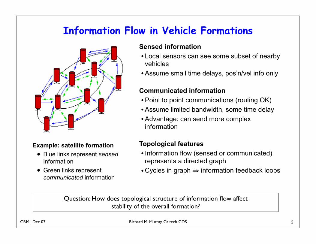
Information Flow in Vehicle Formations

Example: satellite formation• Blue links represent sensed

information

• Green links represent communicated information

Sensed information• Local sensors can see some subset of nearby vehicles•Assume small time delays, pos’n/vel info only

Communicated information•Point to point communications (routing OK)•Assume limited bandwidth, some time delay•Advantage: can send more complex information

Topological features• Information flow (sensed or communicated) represents a directed graph•Cycles in graph ⇒ information feedback loops

Question: How does topological structure of information flow affectstability of the overall formation?


Basic Definitions (1 of 2)

6

Basic Definitions (1/2)

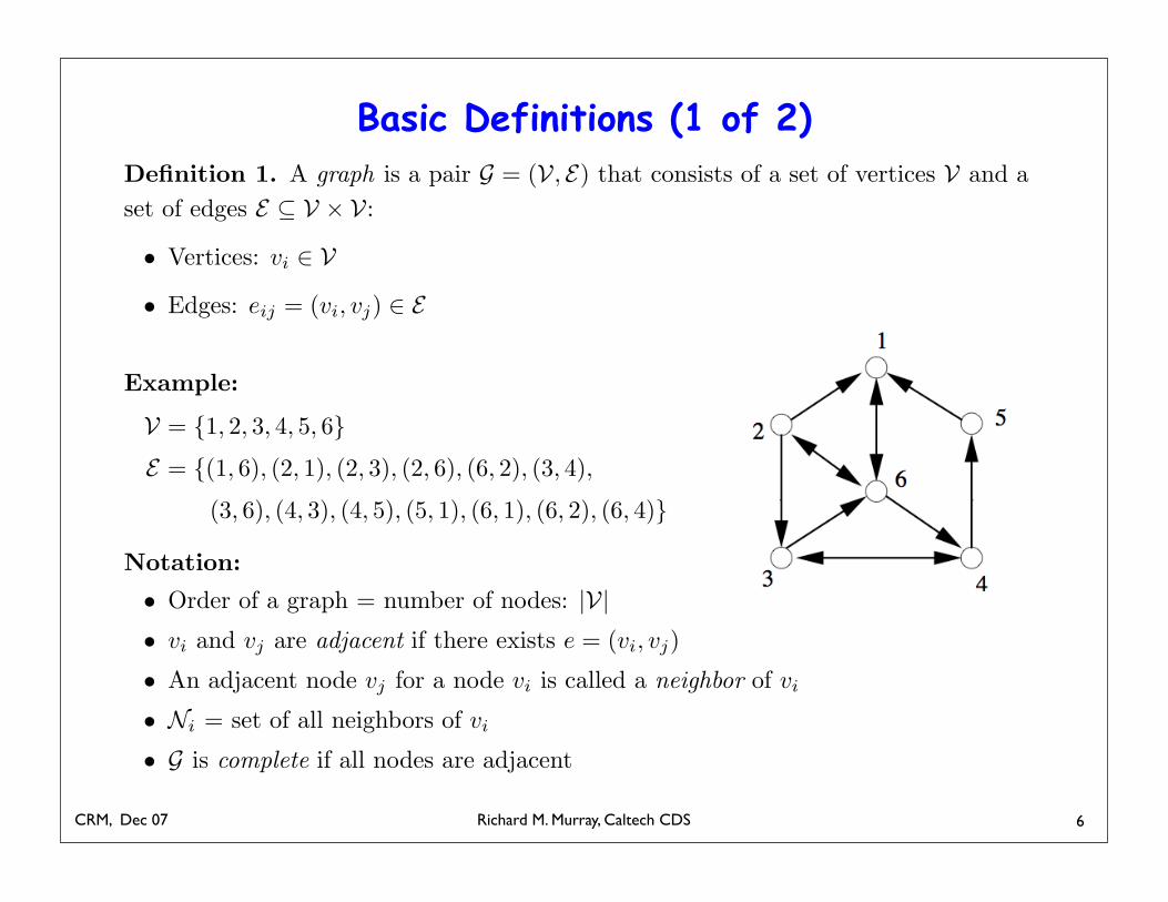
Definition 1. A graph is a pair G = (V, E) that consists of a set of vertices V and a

set of edges E ! V " V:

• Vertices: vi # V

• Edges: eij = (vi, vj) # E

Example:

V = {1, 2, 3, 4, 5, 6}

E = {(1, 6), (2, 1), (2, 3), (2, 6), (6, 2), (3, 4),

(3, 6), (4, 3), (4, 5), (5, 1), (6, 1), (6, 2), (6, 4)}

Notation:

• Order of a graph = number of nodes: |V|

• vi and vj are adjacent if there exists e = (vi, vj)

• An adjacent node vj for a node vi is called a neighbor of vi

• Ni = set of all neighbors of vi

• G is complete if all nodes are adjacent

CRM, 3 Dec 07 R. M. Murray, Caltech CDS 2


Basic Definitions (2 of 2)

7

1

4

6

5 3

2

31 5 9

2 4 8 106

7

2 3

4

1

(a) (b) (c)

Figure 3: Three examples of balanced graphs.

G = (V , E ,A) is called balanced if and only if all of its nodes are balanced, or

!

j

aij =!

j

aji,!i. (22)

Any undirected graph is balanced. Furthermore, the digraphs shown in Figure 3 are allbalanced. Here is our first main result:

Theorem 4. Consider a network of integrators with a fixed topology G = (V , E ,A) that is astrongly connected digraph. Then, protocol (A1) globally asymptotically solves the average-consensus problem if and only if G is balanced.

Proof. The proof follows from Theorems 5 and 6, below.

Remark 6. According to Theorem 4, if a graph is not balanced, then protocol (A1) does not(globally) solve the average consensus-problem for all initial conditions. This assertion isconsistent with the counterexample given in Figure 2.

Theorem 5. Consider a network of integrator agents with a fixed topology G = (V , E ,A)that is a strongly connected digraph. Then, protocol (A1) globally asymptotically solves theaverage-consensus problem if and only if 1T L = 0.

Proof. From Theorem 3, with wr =1"n1 we obtain

x! = limt"+#

x(t) = Rx0 = wr(wTl x0) =

1"n

(wTl x0)1.

This implies Protocol 1 globally exponentially solves a consensus problem with the decisionvalue 1$

n(wTl x0) for each node. If this decision value is equal to Ave(x0),!x0 # Rn, then

necessarily 1$nwl = 1$

n , i.e. wl = wr = 1$n1. This implies that 1 is the left eigenvector of

13

31 2 4 5

678910

31 2 4 5

678910

(a) (b)31 2 4 5

678910

31 2 4 5

678910

(c) (d)

Figure 4: Four examples of balanced and strongly connected digraphs: (a) Ga, (b) Gb, (c)Gc, and (d) Gd satisfying.

as the number of the edges of the graph increases, algebraic connectivity (or !2) increases,and the settling time of the state trajectories decreases.

The case of a directed cycle of length 10, or Ga, has the highest over-shoot. In all fourcases, a consensus is asymptotically reached and the performance is improved as a functionof !2(Gk) for k ! {a, b, c, d}.

In Figure 6(a), a finite automaton is shown with the set of states {Ga, Gb, Gc, Gd} rep-resenting the discrete-states of a network with switching topology as a hybrid system. Thehybrid system starts at the discrete-state Gb and switches every T = 1 second to the nextstate according to the state machine in Figure 6(a). The continuous-time state trajectoriesand the group disagreement (i.e. """2) of the network are shown in Figure 6(b). Clearly, thegroup disagreement is monotonically decreasing. One can observe that an average-consensusis reached asymptotically. Moreover, the group disagreement vanishes exponentially fast.

Next, we present simulation results for the average-consensus problem with communica-tion time-delay for a network with a topology shown in Figure 7. Figure 8 shows the statetrajectories of this network with communication time-delay # for # = 0, 0.5#max, 0.7#max, #max

with #max = $/2!max(Ge) = 0.266. Here, the initial state is a random set of numbers withzero-mean. Clearly, the agreement is achieved for the cases with # < #max in Figures 8(a),(b), and (c). For the case with # = #max, synchronous oscillations are demonstrated in Figure8(d). A third-order Pade approximation is used to model the time-delay as a finite-orderLTI system.

12 Conclusions

We provided the convergence analysis of a consensus protocol for a network of integratorswith directed information flow and fixed/switching topology. Our analysis relies on severaltools from algebraic graph theory, matrix theory, and control theory. We established a con-

22

Basic Definitions (2/2)

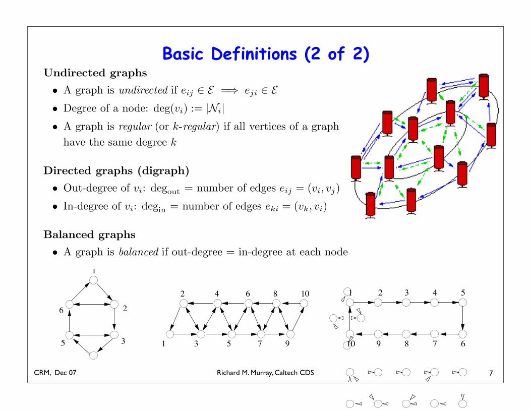
Undirected graphs

• A graph is undirected if eij ! E =" eji ! E

• Degree of a node: deg(vi) := |Ni|

• A graph is regular (or k-regular) if all vertices of a graph

have the same degree k

Directed graphs (digraph)

• Out-degree of vi: degout = number of edges eij = (vi, vj)

• In-degree of vi: degin = number of edges eki = (vk, vi)

Balanced graphs

• A graph is balanced if out-degree = in-degree at each node



Connectedness of Graphs (1 of 2)

8

Connectedness of Graphs (1/2)

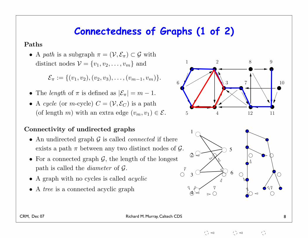
Paths

• A path is a subgraph ! = (V, E!) ! G with

distinct nodes V = {v1, v2, . . . , vm} and

E! := {(v1, v2), (v2, v3), . . . , (vm!1, vm)}.

• The length of ! is defined as |E!| = m " 1.

• A cycle (or m-cycle) C = (V, EC) is a path

(of length m) with an extra edge (vm, v1) # E .

Connectivity of undirected graphs

• An undirected graph G is called connected if there

exists a path ! between any two distinct nodes of G.

• For a connected graph G, the length of the longest

path is called the diameter of G.

• A graph with no cycles is called acyclic

• A tree is a connected acyclic graph


4.3. Algebraic Graph Theory 51

1 2

3

45

6 7

8 9

10

12 11

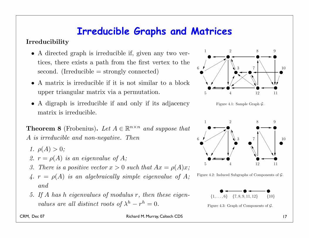
Figure 4.1: Sample Graph G.

1 2

3

45

6 7

8 9

10

12 11

Figure 4.2: Induced Subgraphs of Components of G.

{1, . . . , 6} {7, 8, 9, 11, 12} {10}

Figure 4.3: Graph of Components of G.

1

36

5

2

4

Figure 1.4: A bipartite graph.

For example, the adjacency matrix of the graph in Figure 1.1 is

A =

!

""""""#

0 0 0 0 0 11 0 1 0 0 10 0 0 4 0 10 0 3 0 5 01 0 0 0 0 01 1 0 1 0 0

$

%%%%%%&(1.6)

For sparse graphs that the degree of each node is relatively small compared to the order of thegraph, the adjacency matrix is a rather ine!cient way of representing the graph. Instead, one canuse the neighborhood matrix N in which row i is a list of the elements of Ji plus dmax ! |Ji| zeros(or star marks “*”) where dmax = maxv!V deg(v). For the graph in Figure 1.1, N can be expressedas follows:

N =

!

""""""#

6 0 01 3 64 6 03 5 01 0 01 2 4

$

%%%%%%&(1.7)

Another important matrix in the context of algebraic graph theory [4, 14] is called the incidencematrix C = {cij}. Fix an orientation of the edges of the graph Eo " E and let e1, e2, . . . , em denotethe elements of Eo. Define the elements of the n#m matrix C as

cij :=

'(

)

+1 , vi = h(ej)!1 , vi = t(ej)0 , otherwise.

(1.8)

As an exercise, prove the following property of C.

Lemma 1. The matrix CCT is independent of the choice of the orientation of G.


???

Connectedness of Graphs (2 of 2)

9

Connectedness of Graphs (2/2)

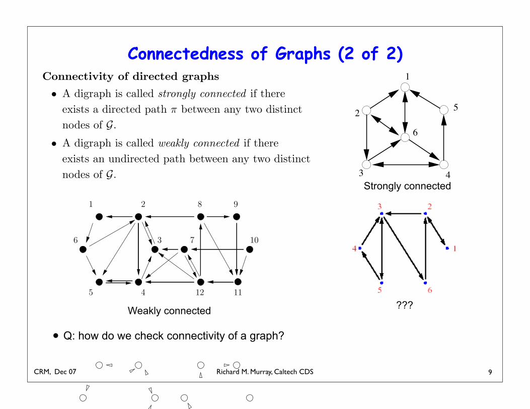
Connectivity of directed graphs

• A digraph is called strongly connected if there

exists a directed path ! between any two distinct

nodes of G.

• A digraph is called weakly connected if there

exists an undirected path between any two distinct

nodes of G.


Chapter 1

Graph Theory

This chapter provides some background on graph theory based on the materials in [7, 5].

1.1 Graphs

A graph is a pair G = (V, E) that consists of a set of vertices V and a set of edges E ! V " V.Each vertex of the graph is denoted by vi or i where i is an index that belongs to an index setI = {1, 2, . . . , n}. Each edge of the graph is denoted by (vi, vj) with i, j # I. Equivalently, fornotational convenience, we sometimes denote (vi, vj) by eij or simply ij. The number of the nodes(or vertices) of a graph is called the order of the graph. This is equal to |V| where for any set S,|S| denotes the number of elements of S. Figure 1.1 shows an example of a graph of order 6 withthe following set of vertices and edges:

V = {1, 2, 3, 4, 5, 6}E = {16, 21, 23, 26, 62, 34, 36, 43, 45, 51, 61, 62, 64} (1.1)

1

2

3 4

5

6

Figure 1.1: A graph of order 6.

1.2 Neighbors of a Node

Two nodes of the graph are called adjacent i! there exists an edge between them. Each adjacentnode vj of the node vi is called the neighbor of vi. The set of all neighbors of vi are denoted by

11


1 2

3

45

6 7

8 9

10

12 11


1 2

3

45

6 7

8 9

10

12 11


{1, . . . , 6} {7, 8, 9, 11, 12} {10}


Strongly connected

Weakly connected

• Q: how do we check connectivity of a graph?


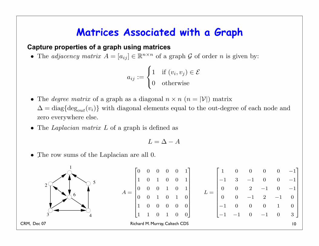
Capture properties of a graph using matrices

Matrices Associated with a Graph

10

Chapter 1

Graph Theory

This chapter provides some background on graph theory based on the materials in [7, 5].

1.1 Graphs

A graph is a pair G = (V, E) that consists of a set of vertices V and a set of edges E ! V " V.Each vertex of the graph is denoted by vi or i where i is an index that belongs to an index setI = {1, 2, . . . , n}. Each edge of the graph is denoted by (vi, vj) with i, j # I. Equivalently, fornotational convenience, we sometimes denote (vi, vj) by eij or simply ij. The number of the nodes(or vertices) of a graph is called the order of the graph. This is equal to |V| where for any set S,|S| denotes the number of elements of S. Figure 1.1 shows an example of a graph of order 6 withthe following set of vertices and edges:

V = {1, 2, 3, 4, 5, 6}E = {16, 21, 23, 26, 62, 34, 36, 43, 45, 51, 61, 62, 64} (1.1)

1

2

3 4

5

6

Figure 1.1: A graph of order 6.

1.2 Neighbors of a Node

Two nodes of the graph are called adjacent i! there exists an edge between them. Each adjacentnode vj of the node vi is called the neighbor of vi. The set of all neighbors of vi are denoted by

11

Matrices Associated with a Graph

• The adjacency matrix A = [aij ] ! Rn!n of a graph G of order n is given by:

aij :=

!

"

#

1 if (vi, vj) ! E

0 otherwise

• The degree matrix of a graph as a diagonal n " n (n = |V|) matrix

! = diag{degout(vi)} with diagonal elements equal to the out-degree of each node and

zero everywhere else.

• The Laplacian matrix L of a graph is defined as

L = ! # A

.• The row sums of the Laplacian are all 0.

A =

2

6

6

6

6

6

6

6

6

6

6

4

0 0 0 0 0 1

1 0 1 0 0 1

0 0 0 1 0 1

0 0 1 0 1 0

1 0 0 0 0 0

1 1 0 1 0 0

3

7

7

7

7

7

7

7

7

7

7

5

L =

2

6

6

6

6

6

6

6

6

6

6

4

1 0 0 0 0 !1

!1 3 !1 0 0 !1

0 0 2 !1 0 !1

0 0 !1 2 !1 0

!1 0 0 0 1 0

!1 !1 0 !1 0 3

3

7

7

7

7

7

7

7

7

7

7

5



Periodic Graphs and Weighted Graphs

11

!

""""""#

1 ! 12 0 0 0 ! 1

2! 1

2 1 ! 12 0 0 0

0 0 1 0 ! 12 ! 1

20 0 !1 1 0 00 0 ! 1

2 ! 12 1 0

0 !1 0 0 0 1

$

%%%%%%&

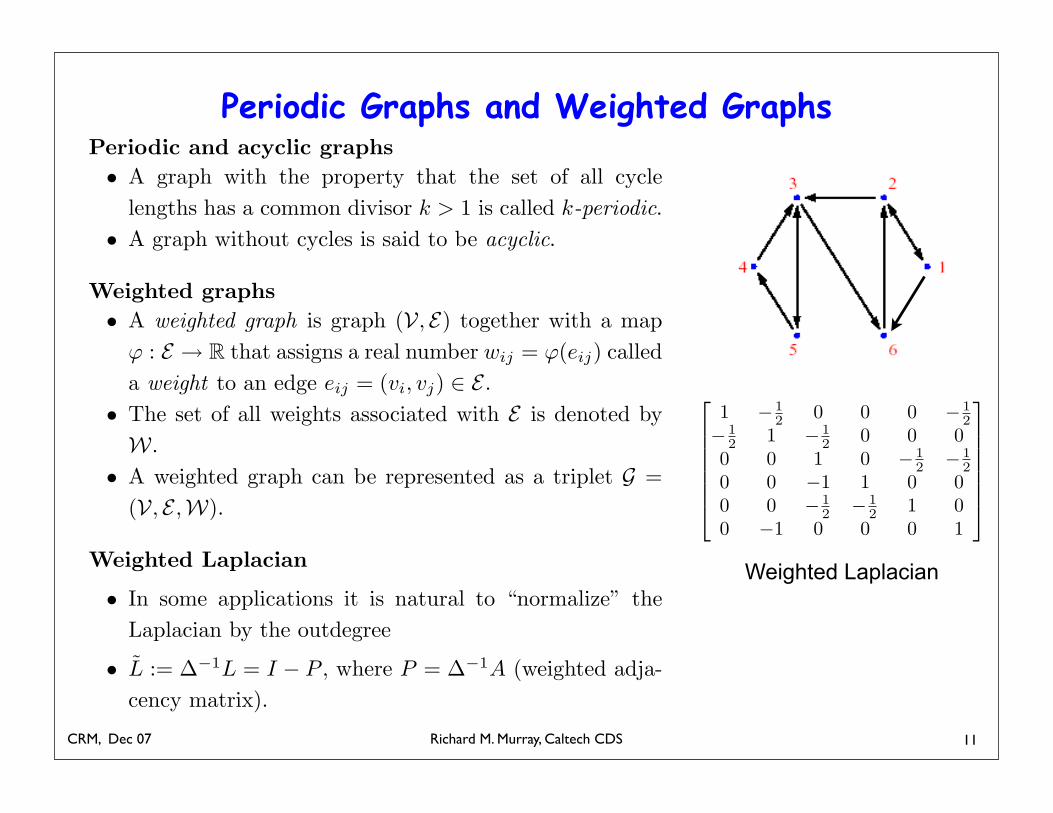
Periodic Graphics and Weighted Graphs

Periodic and acyclic graphs

• A graph with the property that the set of all cycle

lengths has a common divisor k > 1 is called k-periodic.

• A graph without cycles is said to be acyclic.

Weighted graphs

• A weighted graph is graph (V, E) together with a map

! : E ! R that assigns a real number wij = !(eij) called

a weight to an edge eij = (vi, vj) " E .

• The set of all weights associated with E is denoted by

W.

• A weighted graph can be represented as a triplet G =

(V, E ,W).

Weighted Laplacian

• In some applications it is natural to “normalize” the

Laplacian by the outdegree

• L := !!1L = I # P , where P = !!1A (weighted adja-

cency matrix).


Weighted Laplacian


Application: Consensus Protocols

12

0 10 20 30 4010

15

20

25

30

35

40

iteration

xi

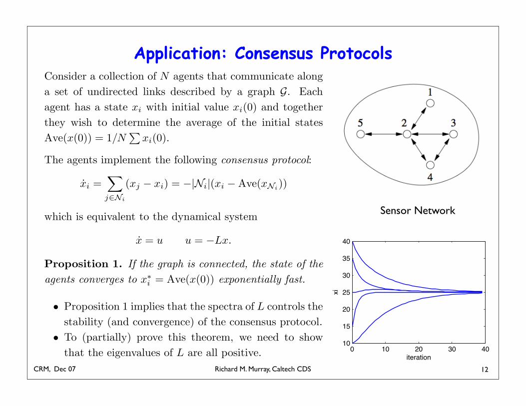
Sensor Network

Consensus protocols

Consider a collection of N agents that communicate along

a set of undirected links described by a graph G. Each

agent has a state xi with initial value xi(0) and together

they wish to determine the average of the initial states

Ave(x(0)) = 1/N!

xi(0).

The agents implement the following consensus protocol:

xi ="

j!Ni

(xj ! xi) = !|Ni|(xi ! Ave(xNi))

which is equivalent to the dynamical system

x = u u = !Lx.

Proposition 1. If the graph is connected, the state of the

agents converges to x"i = Ave(x(0)) exponentially fast.

• Proposition 1 implies that the spectra of L controls the

stability (and convergence) of the consensus protocol.

• To (partially) prove this theorem, we need to show

that the eigenvalues of L are all positive.



Gershgorin Disk Theorem

13

Gershgorin Disk Theorem

Theorem 2 (Gershgorin Disk Theorem). Let A = [aij ] ! Rn!n and define the deleted

absolute row sums of A as

ri :=n

!

j=1,j "=i

|aij | (1)

Then all the eigenvalues of A are located in the union of n disks

G(A) :=n"

i=1

Gi(A), with Gi(A) := {z ! C : |z " aii| # ri} (2)

Furthermore, if a union of k of these n disks forms a connected region that is disjoint from

all the remaining n " k disks, then there are precisely k eigenvalues of A in this region.

Sketch of proof Let ! be an eigenvalue of A and let v be a corresponding eigenvector.

Choose i such that |vi| = maxj |vj > 0. Since v is an eigenvector,

!vi =!

i

Aijvj =$ (! " aii)vi =!

i "=j

Aijvj

Now divide by vi %= 0 and take the absolute value to obtain

|! " aii| = |!

j "=i

aijvj | #!

j "=i

|aij | = ri



Properties of the Laplacian (1)

14

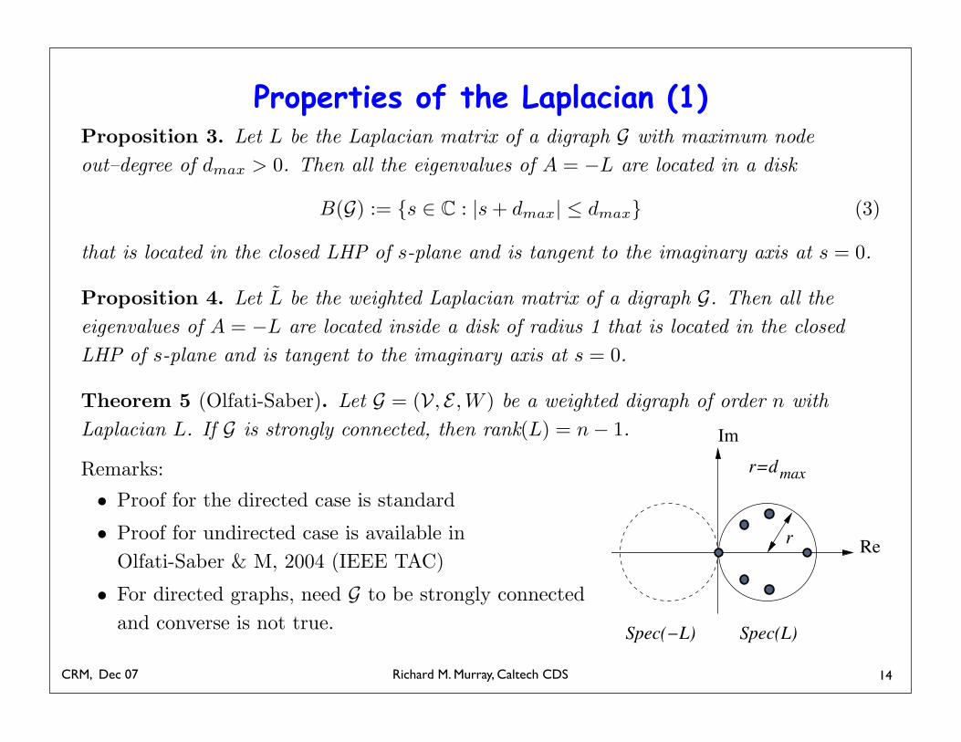
Properties of the Laplacian (1)

Proposition 3. Let L be the Laplacian matrix of a digraph G with maximum node

out–degree of dmax > 0. Then all the eigenvalues of A = !L are located in a disk

B(G) := {s " C : |s + dmax| # dmax} (3)

that is located in the closed LHP of s-plane and is tangent to the imaginary axis at s = 0.

Proposition 4. Let L be the weighted Laplacian matrix of a digraph G. Then all the

eigenvalues of A = !L are located inside a disk of radius 1 that is located in the closed

LHP of s-plane and is tangent to the imaginary axis at s = 0.

Theorem 5 (Olfati-Saber). Let G = (V, E , W ) be a weighted digraph of order n with

Laplacian L. If G is strongly connected, then rank(L) = n ! 1.

Remarks:

• Proof for the directed case is standard

• Proof for undirected case is available in

Olfati-Saber & M, 2004 (IEEE TAC)

• For directed graphs, need G to be strongly connected

and converse is not true.


Remark 5. The notion of algebraic connectivity (or !2) of graphs was originally defined byM. Fiedler for undirected graphs [13, 14]. We extend this notion to algebraic connectivity ofdigraphs by defining the mirror operation on digraphs that produces an undirected graph Gfrom a digraph G (See Definition 2).

The key in the stability analysis of system (8) is in the spectral properties of graphLaplacian. The following result is well-known for undirected graphs (e.g. see [26]). Here, westate the result for digraphs and prove it using Gersgorin disk theorem [19].

Spec(L)Spec(!L)

r

Im

Re

r=d max

Figure 1: A demonstration of Gersgorin Theorem applied to graph Laplacian.

Theorem 2. (spectral localization) Let G = (V , E ,A) be a digraph with the Laplacian L.Denote the maximum node out-degree of the digraph G by dmax(G) = maxi degout(vi). Then,all the eigenvalues of L = L(G) are located in the following disk

D(G) = {z ! C : |z " dmax(G)| # dmax(G)} (18)

centered at z = dmax(G) + 0j in the complex plane (see Figure 1).

Proof. Based on the Gersgorin disk theorem, all the eigenvalues of L = [lij] are located inthe union of the following n disks

Di = {z ! C : |z " lii| #!

j!I,j "=i

|lij|}. (19)

But for the digraph G, lii = !ii and

!

j!I,j "=i

|lij| = degout(vi) = !ii.

Thus, Di = {z ! C : |z "!ii| # !ii}. On the other hand, all these n disks are contained inthe largest disk D(G) with radius dmax(G). Clearly, all the eigenvalues of "L are located inthe disk D#(G) = {z ! C : |z + dmax(G)| # dmax(G)} that is the mirror image of D(G) withrespect to the imaginary axis.

10


Proof of the Consensus Protocol

15

Proof of Consensus Protocol

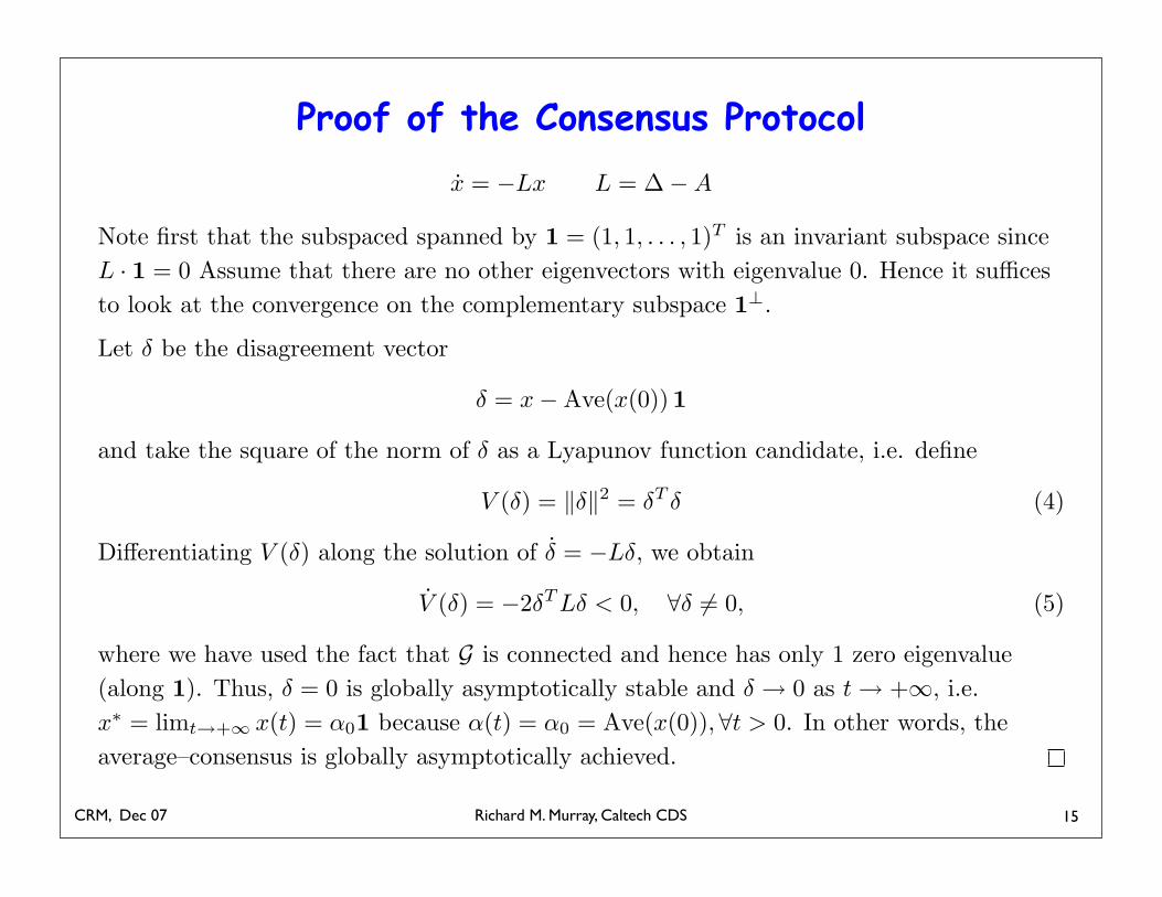
x = !Lx L = ! ! A

Note first that the subspaced spanned by 1 = (1, 1, . . . , 1)T is an invariant subspace since

L · 1 = 0 Assume that there are no other eigenvectors with eigenvalue 0. Hence it su"ces

to look at the convergence on the complementary subspace 1!.

Let ! be the disagreement vector

! = x ! Ave(x(0))1

and take the square of the norm of ! as a Lyapunov function candidate, i.e. define

V (!) = "!"2 = !T ! (4)

Di#erentiating V (!) along the solution of ! = !L!, we obtain

V (!) = !2!T L! < 0, #! $= 0, (5)

where we have used the fact that G is connected and hence has only 1 zero eigenvalue

(along 1). Thus, ! = 0 is globally asymptotically stable and ! % 0 as t % +&, i.e.

x" = limt#+$ x(t) = "01 because "(t) = "0 = Ave(x(0)),#t > 0. In other words, the

average–consensus is globally asymptotically achieved.



Perron-Frobenius Theory

16

Perron-Frobenius Theory

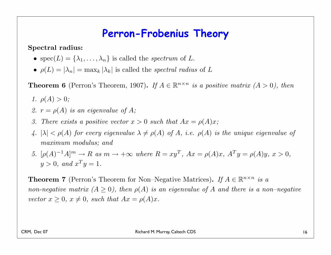
Spectral radius:

• spec(L) = {!1, . . . , !n} is called the spectrum of L.

• "(L) = |!n| = maxk |!k| is called the spectral radius of L

Theorem 6 (Perron’s Theorem, 1907). If A ! Rn!n is a positive matrix (A > 0), then

1. "(A) > 0;

2. r = "(A) is an eigenvalue of A;

3. There exists a positive vector x > 0 such that Ax = "(A)x;

4. |!| < "(A) for every eigenvalue ! "= "(A) of A, i.e. "(A) is the unique eigenvalue of

maximum modulus; and

5. ["(A)"1A]m # R as m # +$ where R = xyT , Ax = "(A)x, AT y = "(A)y, x > 0,

y > 0, and xT y = 1.

Theorem 7 (Perron’s Theorem for Non–Negative Matrices). If A ! Rn!n is a

non-negative matrix (A % 0), then "(A) is an eigenvalue of A and there is a non–negative

vector x % 0, x "= 0, such that Ax = "(A)x.



Irreducible Graphs and Matrices

17


1 2

3

45

6 7

8 9

10

12 11


1 2

3

45

6 7

8 9

10

12 11


{1, . . . , 6} {7, 8, 9, 11, 12} {10}


Irreducible Graphs and Matrices

Irreducibility

• A directed graph is irreducible if, given any two ver-

tices, there exists a path from the first vertex to the

second. (Irreducible = strongly connected)

• A matrix is irreducible if it is not similar to a block

upper triangular matrix via a permutation.

• A digraph is irreducible if and only if its adjacency

matrix is irreducible.

Theorem 8 (Frobenius). Let A ! Rn!n and suppose that

A is irreducible and non-negative. Then

1. !(A) > 0;

2. r = !(A) is an eigenvalue of A;

3. There is a positive vector x > 0 such that Ax = !(A)x;

4. r = !(A) is an algebraically simple eigenvalue of A;

and

5. If A has h eigenvalues of modulus r, then these eigen-

values are all distinct roots of "h " rh = 0.



Properties of Laplacians (2)

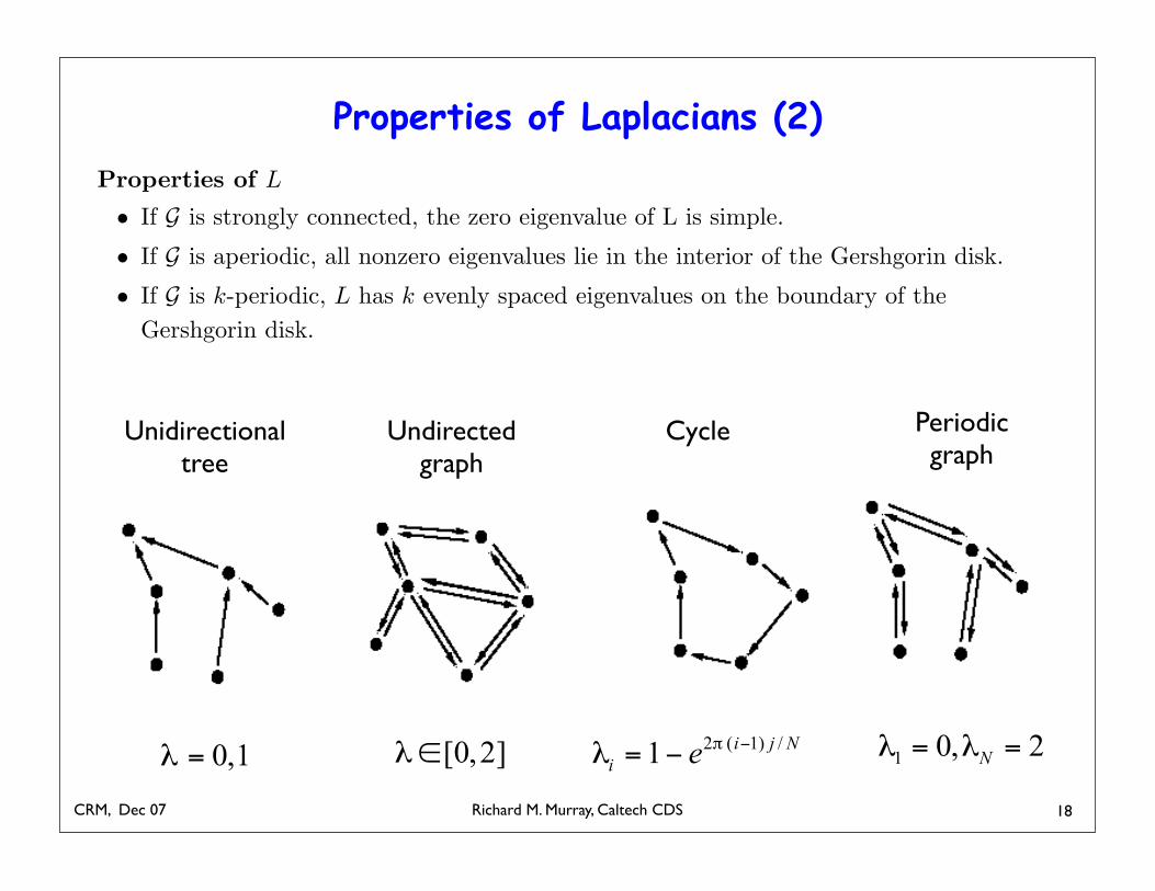
Unidirectionaltree

CycleUndirected graph

Periodicgraph

Spectra of the Laplacian

Properties of L

• If G is strongly connected, the zero eigenvalue of L is simple.

• If G is aperiodic, all nonzero eigenvalues lie in the interior of the Gershgorin disk.

• If G is k-periodic, L has k evenly spaced eigenvalues on the boundary of the

Gershgorin disk.



Algebraic Connectivity

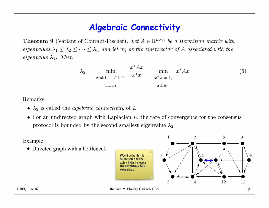
Example• Directed graph with a bottleneck

19


1 2

3

45

6 7

8 9

10

12 11


1 2

3

45

6 7

8 9

10

12 11


{1, . . . , 6} {7, 8, 9, 11, 12} {10}


Algebraic Connectivity

Theorem 9 (Variant of Courant-Fischer). Let A ! Rn!n be a Hermitian matrix with

eigenvalues !1 " !2 " · · · " !n and let w1 be the eigenvector of A associated with the

eigenvalue !1. Then

!2 = minx != 0, x " Cn

,

x#w1

x"Ax

x"x= min

x!x = 1,

x#w1

x"Ax (6)

Remarks:

• !2 is called the algebraic connectivity of L

• For an undirected graph with Laplacian L, the rate of convergence for the consensus

protocol is bounded by the second smallest eigenvalue !2


Would be better to delete some of the extra links to make the bottleneck link more clear.


Cyclically Separable Graphs

20

1

4

6

5 3

2

31 5 9

2 4 8 106

7

2 3

4

1

(a) (b) (c)



!

j

aij =!

j

aji,!i. (22)







x! = limt"+#


1"n

(wTl x0)1.





13

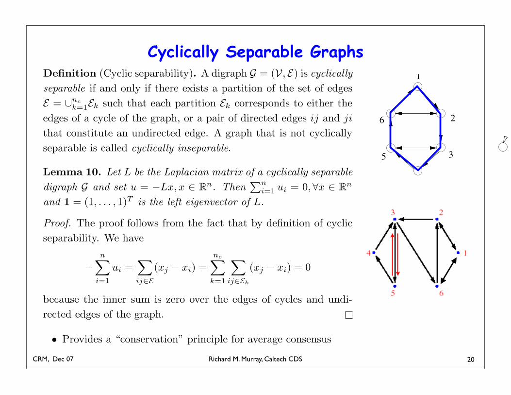
Cyclically Separable Graphs

Definition (Cyclic separability). A digraph G = (V, E) is cyclically

separable if and only if there exists a partition of the set of edges

E = !nc

k=1Ek such that each partition Ek corresponds to either the

edges of a cycle of the graph, or a pair of directed edges ij and ji

that constitute an undirected edge. A graph that is not cyclically

separable is called cyclically inseparable.

Lemma 10. Let L be the Laplacian matrix of a cyclically separable

digraph G and set u = "Lx, x # Rn. Then!n

i=1ui = 0,$x # Rn

and 1 = (1, . . . , 1)T is the left eigenvector of L.

Proof. The proof follows from the fact that by definition of cyclic

separability. We have

"n

"

i=1

ui ="

ij!E

(xj " xi) =nc"

k=1

"

ij!Ek

(xj " xi) = 0

because the inner sum is zero over the edges of cycles and undi-

rected edges of the graph.

• Provides a “conservation” principle for average consensus



Balanced Graphs

21

1

4

6

5 3

2

31 5 9

2 4 8 106

7

2 3

4

1

(a) (b) (c)



!

j

aij =!

j

aji,!i. (22)







x! = limt"+#


1"n

(wTl x0)1.





13

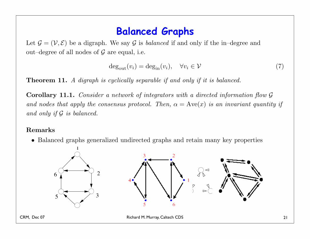
Consensus on Balanced Graphs

Let G = (V, E) be a digraph. We say G is balanced if and only if the in–degree and

out–degree of all nodes of G are equal, i.e.

degout(vi) = degin(vi), !vi " V (7)

Theorem 11. A digraph is cyclically separable if and only if it is balanced.

Corollary 11.1. Consider a network of integrators with a directed information flow G

and nodes that apply the consensus protocol. Then, ! = Ave(x) is an invariant quantity if

and only if G is balanced.

Remarks

• Balanced graphs generalized undirected graphs and retain many key properties



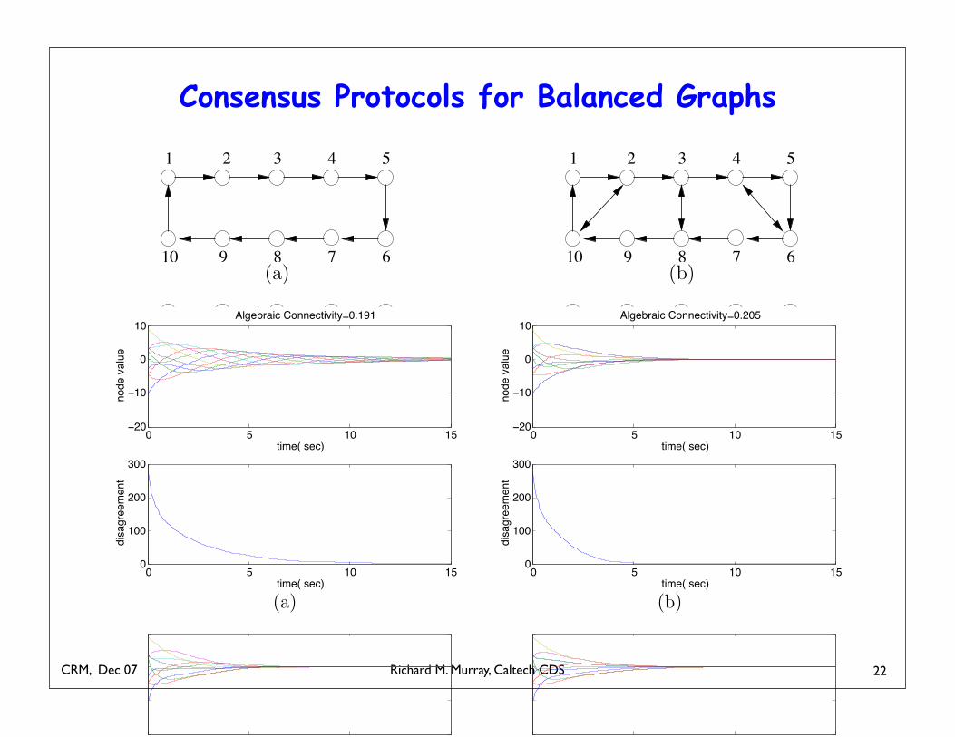
Consensus Protocols for Balanced Graphs

22

31 2 4 5

678910

31 2 4 5

678910

(a) (b)31 2 4 5

678910

31 2 4 5

678910

(c) (d)

Figure 4: Four examples of balanced and strongly connected digraphs: (a) Ga, (b) Gb, (c)Gc, and (d) Gd satisfying.

as the number of the edges of the graph increases, algebraic connectivity (or !2) increases,and the settling time of the state trajectories decreases.

The case of a directed cycle of length 10, or Ga, has the highest over-shoot. In all fourcases, a consensus is asymptotically reached and the performance is improved as a functionof !2(Gk) for k ! {a, b, c, d}.

In Figure 6(a), a finite automaton is shown with the set of states {Ga, Gb, Gc, Gd} rep-resenting the discrete-states of a network with switching topology as a hybrid system. Thehybrid system starts at the discrete-state Gb and switches every T = 1 second to the nextstate according to the state machine in Figure 6(a). The continuous-time state trajectoriesand the group disagreement (i.e. """2) of the network are shown in Figure 6(b). Clearly, thegroup disagreement is monotonically decreasing. One can observe that an average-consensusis reached asymptotically. Moreover, the group disagreement vanishes exponentially fast.

Next, we present simulation results for the average-consensus problem with communica-tion time-delay for a network with a topology shown in Figure 7. Figure 8 shows the statetrajectories of this network with communication time-delay # for # = 0, 0.5#max, 0.7#max, #max

with #max = $/2!max(Ge) = 0.266. Here, the initial state is a random set of numbers withzero-mean. Clearly, the agreement is achieved for the cases with # < #max in Figures 8(a),(b), and (c). For the case with # = #max, synchronous oscillations are demonstrated in Figure8(d). A third-order Pade approximation is used to model the time-delay as a finite-orderLTI system.

12 Conclusions

We provided the convergence analysis of a consensus protocol for a network of integratorswith directed information flow and fixed/switching topology. Our analysis relies on severaltools from algebraic graph theory, matrix theory, and control theory. We established a con-

22

0 5 10 15!20

!10

0

10Algebraic Connectivity=0.191

time( sec)

node v

alu

e

0 5 10 150

100

200

300

time( sec)

dis

agre

em

ent

0 5 10 15!20

!10

0


time( sec)

node v

alu

e

0 5 10 150

100

200

300

time( sec)

dis

agre

em

ent

(a) (b)

0 5 10 15!20

!10

0


time( sec)

node v

alu

e

0 5 10 150

100

200

300

time( sec)

dis

agre

em

ent

0 5 10 15!20

!10

0


time( sec)

node v

alu

e

0 5 10 150

100

200

300

time( sec)

dis

agre

em

ent

(c) (d)

Figure 5: For examples of balanced and strongly connected digraphs: (a) Ga, (b) Gb, (c) Gc,and (d) Gd satisfying.

nection between the performance of a linear consensus protocol and the Fiedler eigenvalue ofthe mirror graph of a balanced digraph. This provides an extension of the notion of algebraicconnectivity of graphs to algebraic connectivity of balanced digraphs. A simple disagreementfunction was introduced as a Lyapunov function for the group disagreement dynamics. Thiswas later used to provide a common Lyapunov function that allowed convergence analysis ofan agreement protocol for a network with switching topology. A commutative diagram wasgiven that shows the operations of taking Laplacian and symmetric part of a matrix commutefor adjacency matrix of balanced graphs. Balanced graphs turned out to be instrumental insolving average-consensus problems.

For undirected networks with fixed topology, we gave su!cient and necessary condi-tions for reaching an average-consensus in presence of communication time-delays. It was

23


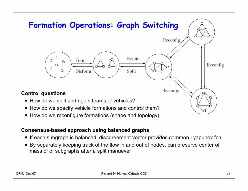
Formation Operations: Graph Switching

Control questions• How do we split and rejoin teams of vehicles?• How do we specify vehicle formations and control them?• How do we reconfigure formations (shape and topology)

Consensus-based approach using balanced graphs• If each subgraph is balanced, disagreement vector provides common Lyapunov fcn• By separately keeping track of the flow in and out of nodes, can preserve center of

mass of of subgraphs after a split manuever


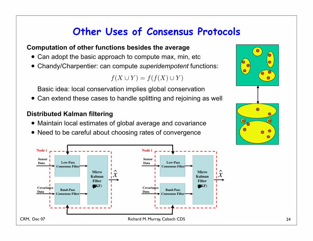
Other Uses of Consensus ProtocolsComputation of other functions besides the average• Can adopt the basic approach to compute max, min, etc• Chandy/Charpentier: can compute superidempotent functions:

Basic idea: local conservation implies global conservation• Can extend these cases to handle splitting and rejoining as well

Distributed Kalman filtering• Maintain local estimates of global average and covariance• Need to be careful about choosing rates of convergence

24

f(X ! Y ) = f(f(X) ! Y )

8 Reza Olfati-Saber

with a state (ei, qi) ! R2m, input ui, and output qi. This filter is used forinverse-covariance consensus that calculates Si column-wise for node i byapplying the filter on columns of H !

iR"1i Hi as the inputs of node i. The

matrix version of this filter can take H !iR

"1i Hi as the input.

Fig. 2 shows the architecture of each node of the sensor network for dis-tributed Kalman filtering. Note that consensus filtering is performed with thesame frequency as Kalman filtering. This is a unique feature that completelydistinguishes our algorithm with some related work in [30, 33].

Sensor

Data

Covariance

Data

Low-Pass

Consensus Filter

Band-Pass

Consensus Filter

Micro

Kalman

Filter

(µKF)

Node i

x

(a) (b)

Fig. 2. Node and network architecture for distributed Kalman filtering: (a) archi-tecture of consensus filters and µKF of a node and (b) communication patternsbetween low-pass/band-pass consensus filters of neighboring nodes.

5 Simulation Results

In this section, we use our consensus filters jointly with the update equationof the micro-Kalman filter of each node to obtain an estimate of the positionof a moving object in R2 that (approximately) goes in circles. The outputmatrix is Hi = I2 and the state of the process dynamics is 2-dimensionalcorresponding to the continuous-time system

x = A0x + B0w

8 Reza Olfati-Saber

with a state (ei, qi) ! R2m, input ui, and output qi. This filter is used forinverse-covariance consensus that calculates Si column-wise for node i byapplying the filter on columns of H !

iR"1i Hi as the inputs of node i. The

matrix version of this filter can take H !iR

"1i Hi as the input.

Fig. 2 shows the architecture of each node of the sensor network for dis-tributed Kalman filtering. Note that consensus filtering is performed with thesame frequency as Kalman filtering. This is a unique feature that completelydistinguishes our algorithm with some related work in [30, 33].

Sensor

Data

Covariance

Data

Low-Pass

Consensus Filter

Band-Pass

Consensus Filter

Micro

Kalman

Filter

(µKF)

Node i

x

(a) (b)

Fig. 2. Node and network architecture for distributed Kalman filtering: (a) archi-tecture of consensus filters and µKF of a node and (b) communication patternsbetween low-pass/band-pass consensus filters of neighboring nodes.

5 Simulation Results

In this section, we use our consensus filters jointly with the update equationof the micro-Kalman filter of each node to obtain an estimate of the positionof a moving object in R2 that (approximately) goes in circles. The outputmatrix is Hi = I2 and the state of the process dynamics is 2-dimensionalcorresponding to the continuous-time system

x = A0x + B0w


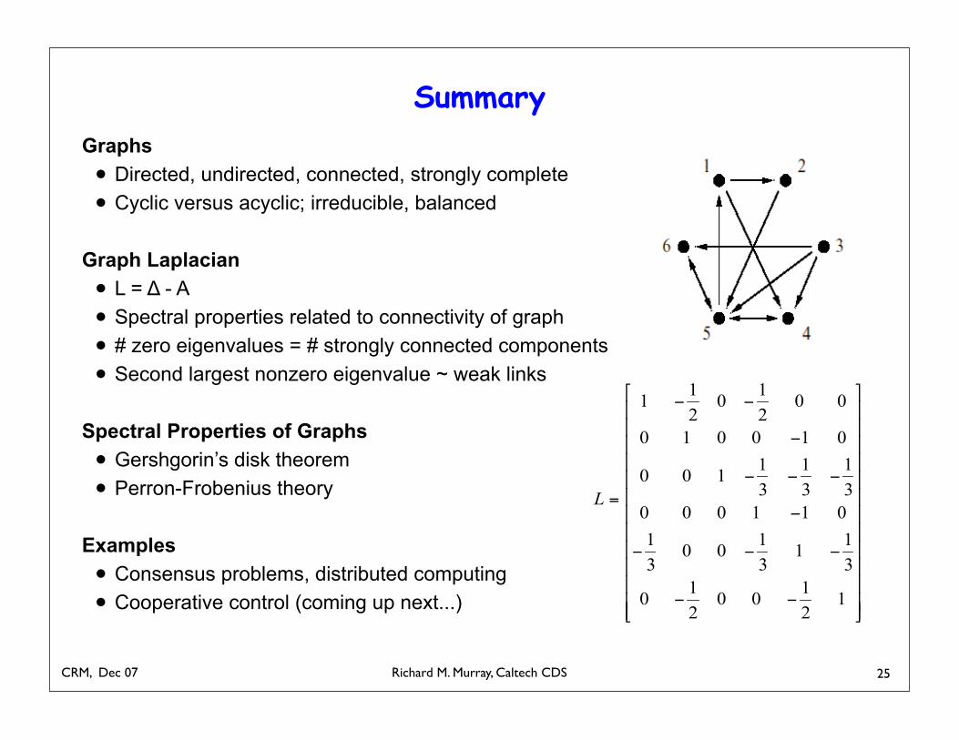
SummaryGraphs• Directed, undirected, connected, strongly complete• Cyclic versus acyclic; irreducible, balanced

Graph Laplacian• L = Δ - A• Spectral properties related to connectivity of graph• # zero eigenvalues = # strongly connected components• Second largest nonzero eigenvalue ~ weak links

Spectral Properties of Graphs• Gershgorin’s disk theorem• Perron-Frobenius theory

Examples• Consensus problems, distributed computing• Cooperative control (coming up next...)

25

Documents

A Primer on Graph Theory - Centro di Ricerca Matematica ...crm.sns.it/media/course/1518/murray-graphtheory.pdf · A Primer on Graph Theory Richard M. Murray Control and Dynamical